Seiberg-Witten Geometry

via Confining Phase Superpotential

Seiji TERASHIMA

A dissertation submitted to the Doctoral Programin Physics, the University of Tsukuba

in partial fulfillment of the requirements for thedegree of Doctor of Philosophy (Science)

January, 1999

Abstract

We study Seiberg-Witten Geometry to describe the non-perturbative low-energy be-

havior of N = 2 supersymmetric gauge theories in four dimensions. The method of N = 1

confining phase superpotential is employed for this purpose. It is shown that the ALE

space of type ADE fibered over CP1 is natural geometry for the N = 2 supersymmetric

gauge theories with ADE gauge groups. Furthermore, we obtain in this approach previ-

ously unknown Seiberg-Witten geometry for four-dimensional N = 2 gauge theory with

gauge group E6 with massive fundamental hypermultiplets. By considering the gauge

symmetry breaking in this E6 gauge theory, we also obtain Seiberg-Witten geometries for

N = 2 gauge theory with SO(2Nc) (Nc ≤ 5) with massive spinor and vector hypermul-

tiplets. In a similar way the Seiberg-Witten geometry is determined for N = 2 SU(Nc)

(Nc ≤ 6) gauge theory with massive antisymmetric and fundamental hypermultiplets.

Contents

1 Introduction 2

2 Seiberg-Witten Geometry 8

2.1 Seiberg-Witten curve . . . . . . . . . . . . . . . . . . . . . . . . . . . . . . 8

2.2 Seiberg-Witten geometry . . . . . . . . . . . . . . . . . . . . . . . . . . . . 12

3 Confining Phase Superpotential 16

3.1 Simplest example: SU(2) gauge theory . . . . . . . . . . . . . . . . . . . . 16

3.2 Outline of confining phase superpotential . . . . . . . . . . . . . . . . . . . 17

4 N = 2 Pure Yang-Mills Theory 21

4.1 Classical gauge groups . . . . . . . . . . . . . . . . . . . . . . . . . . . . . 21

4.2 ADE gauge groups . . . . . . . . . . . . . . . . . . . . . . . . . . . . . . . 31

4.2.1 N = 1 superconformal field theory . . . . . . . . . . . . . . . . . . . 38

5 N = 2 Gauge Theory with Matter Multiplets 42

5.1 Classical gauge groups and fundamental matters . . . . . . . . . . . . . . . 42

5.2 ADE gauge groups and various matters . . . . . . . . . . . . . . . . . . . . 50

5.2.1 E6 theory with fundamental matters . . . . . . . . . . . . . . . . . 56

5.2.2 Gauge symmetry breaking in Seiberg-Witten geometry . . . . . . . 64

5.2.3 Breaking E6 gauge group to SO(10) . . . . . . . . . . . . . . . . . . 68

5.2.4 Breaking E6 gauge group to SU(6) . . . . . . . . . . . . . . . . . . 73

6 Conclusions 78

1

Chapter 1

Introduction

For almost 25 years four-dimensional supersymmetric gauge field theories have been in-

vestigated very intensively. One reason for this is that supersymmetric theories have a

remarkable property of canceling out the divergence in the self-energies which is desir-

able to construct a more natural phenomenological model at high energies beyond the

standard model. Furthermore a proposal of the unification of the gauge groups of the

standard model seems to be more attractive by requiring the theory to have softly broken

supersymmetry.

Supersymmetric gauge theories have also been considered as theoretical models to un-

derstand the strong coupling effects. These effects such as color confinement and chiral

symmetry breaking are difficult to study analytically in the theories without the super-

symmetry. On the other hand the action of the supersymmetric field theory is highly

constrained by its supersymmetry and in some cases even the exact descriptions of the

low-energy theories of these have been obtained on the basis of the idea of duality and

holomorphy [1]-[4]. Consequently, the non-perturbative effects in the supersymmetric

theory can be evaluated quantitatively.

Another reason for the importance of the study of supersymmetric gauge field theories

is their close relation to the superstring theory. Superstring theories receive a lot of

current research interest since they are the only known unified models including quantum

gravity in a consistent manner and have enough gauge symmetries to contain the standard

model. Moreover the superstring theory predicts the spacetime supersymmetry. Therefore

supersymmetric gauge field theories naturally appear in the study of the superstring

2

theory.

In the superstring theory, the supersymmetric gauge field theories appear in two ways.

A conventional way is to have a supersymmetric field theory on the lower dimensional

spacetime after the ten-dimensional superstring is compactified. The other novel way

is that supersymmetric gauge theories in various dimensions are realized on the world

volume of D-branes which are higher dimensional objects on which the open strings can

end. In the framework of the superstring theory, the gauge field theories with extended

supersymmetry ∗ are important because ten-dimensional superstring theories have more

supercharges than lower-dimensional N = 1 (i.e. minimal) supersymmetric theory and

some or all of these supercharges are unbroken if we compactify the superstring theory

on a suitably chosen manifold.

In the case of N = 2 supersymmetry, a substantial progress was made by Seiberg

and Witten [3, 4]. They have shown that the low-energy effective theory of the Coulomb

phase of four-dimensional N = 2 supersymmetric SU(2) gauge theory can be described

by an auxiliary complex curve, called the Seiberg-Witten curve, whose shape depends

on the vacuum moduli u = Tr Φ2. In this beautiful mathematical description, massless

solitons are recognized as vanishing cycles associated with the degeneracy of the curves

and their masses are obtained as the integral of certain one-form, which is called the

Seiberg-Witten form, over these cycles. Soon after these works, generalizations to the

other N = 2 supersymmetric gauge theory with the classical gauge groups have been

carried out by several groups [5]-[12]. However all these generalizations are based on

the assumption that auxiliary complex curves are of hyperelliptic type. Without this

assumption, simple extensions of the original work [3, 4] are not promising to determine

the curves. Thus it is desired to invent other methods for deriving the curve without the

assumption on the types of curves.

To this end, we notice the fact that the singularity of quantum moduli space of the

vacua of the theory corresponds to the appearance of massless solitons. Near the singular-

ity, therefore, we observe interesting non-perturbative properties of the theories. Moreover

∗Here the extended supersymmetric theory has more supercharges than minimal supersymmetric the-ory (N = 1 supersymmetry). For example, the N = 2 supersymmetry is two times as large as the N = 1supersymmetry

3

the Seiberg-Witten curves are determined almost completely from the information of the

locations of singularities on the moduli space. In order to explore physics near N = 2

singularities the microscopic superpotential explicitly breaking N = 2 to N = 1 super-

symmetry is often considered [3, 4, 13, 14]. Examining the resulting superpotential for a

low-energy effective Abelian theory it is found that the generic N = 2 vacuum is lifted

and only the singular loci of moduli space remain as the N = 1 vacua where monopoles

or dyons can condense. The resulting N = 1 theory is shown to be in the confining phase

in accordance with the old idea of the confinement via the condensation of monopole.

This observation suggests that we may start with a microscopic N = 1 theory which we

introduce by perturbing an N = 2 theory by adding a tree-level superpotential built out of

the Casimirs of the adjoint field in the vector multiplet [13, 15, 16] toward the construction

of the N = 2 curves. Let us concentrate on a phase with a single confined photon in our

N = 1 theory which corresponds to the classical SU(2)×U(1)r−1 vacua with r being the

rank of the gauge group. Then the low-energy effective theory containing non-perturbative

effects provides us with the data of the vacua with massless solitons [17, 13]. From this

we can identify the singular points in the Coulomb phase of N = 2 theories and construct

the N = 2 Seiberg-Witten curves. This idea, called ”confining phase superpotential

technique”, has been successfully applied to N = 2 supersymmetric SU(Nc) pure Yang-

Mills theory [15]. We extend their result to the case of N = 2 supersymmetric pure Yang-

Mills theory with arbitrary classical gauge group [19] as well as N = 2 supersymmetric

QCD [21] (see also [13]-[20]). The resulting curves are hyperelliptic type and agree with

those of [7]-[12].

On the other hand, for exceptional gauge groups there were proposals based on the

relation between Seiberg-Witten theory and the integrable systems that Seiberg-Witten

curves are not realized by hyperelliptic curves [23, 24, 25]. In [23] it is claimed that

the Seiberg-Witten curves for the N = 2 supersymmetric pure Yang-Mills theory with

arbitrary simple gauge group are given by the spectral curves for the affine Toda lattice

which has a form of a foliation over CP1. For G2 gauge group, this has been confirmed

by the confining phase superpotential [26] and the one instanton calculation [27].

The application of the confining phase superpotential technique to the E6, E7, E8 gauge

groups seems to be difficult at first sight because of the complicated structure of the

4

En groups. Nonetheless we have shown that this technique can be applied in a unified

way in determining the singularity structure of moduli space of the Coulomb phase in

supersymmetric pure Yang-Mills theories with ADE gauge groups [28]. Not only the

classical case of Ar, Dr groups but the exceptional case of E6, E7, E8 groups can be treated

on an equal footing since our discussion is based on the fundamental properties of the

root system of the simply-laced Lie algebras. The resulting Riemann surface is described

as a foliation over CP1 and satisfies the singularity conditions we have obtained from the

N = 1 confining phase superpotential. This Riemann surface is not of hyperelliptic type

for exceptional gauge groups.

In the consideration within the scope of four-dimensional field theory, it was unclear

if the Riemann surface in the exact description is an auxiliary object for mathematical

setup or a real physical object. It turns out that four-dimensional N = 2 gauge theory

on R4 is realized in the type IIA superstring theory by an Neveu-Schwarz fivebrane on

R4×Σ where Σ is the Seiberg-Witten curve [29]. (This fivebrane description of the gauge

theory is more transparent in view of 11 dimensional M theory [30].) The T-dual of this

curved fivebrane configuration is obtained as type IIB superstring theory compactified on a

Calabi-Yau three-fold which is a compact complex Kahler manifold of complex dimension

three with vanishing first Chern class. Here we should take this Calabi-Yau three-fold

to be a form of K3 fibration over CP1 with a certain limit which implies the decoupling

of gravity. The singularities of K3, where some two-cycles get shrinked, are classified by

the ADE singularity types and the gauge group of four-dimensional theory corresponds

to these ADE singularities of K3. From the point of view of four-dimensional theory,

this limiting Calabi-Yau three-fold is considered as a higher dimensional generalization

of the auxiliary Seiberg-Witten curve and called Seiberg-Witten geometry. For ADE

type gauge groups, this Seiberg-Witten geometry may be a more natural object than the

curve since the curve depends on the representation of the gauge group, furthermore,

there are the Seiberg-Witten geometries which are difficult to be reduced to the curve.

Surprisingly it has been shown that this Seiberg-Witten geometry of the form of ADE

singularity fibration over CP1 naturally appears in the framework of the confining phase

superpotential [28, 31, 32] despite that this method has no relation to K3 or Calabi-Yau

manifold at first sight.

5

Some extension to include matter hypermultiplets in representations other than the

fundamentals can be also considered as the compactification on the Calabi-Yau three-

fold [33, 34]. In his approach, however, only massless matters have been treated and

the representation of matters are very restricted. On the other hand, the technique

of confining phase superpotential can be also applied to supersymmetric theories with

matter hypermultiplets and be used to investigate wider class of the theory. Indeed we

have succeeded in deriving previously unknown Seiberg-Witten geometries for the N = 2

theory with E6 gauge group with the massive fundamental hypermultiplets [31]. Moreover

breaking the E6 symmetry down to SO(2Nc) (Nc ≤ 5), we derive the Seiberg-Witten

geometry for N = 2 SO(2Nc) theory with massive spinor and vector hypermultiplets [32].

In the massless limit, our SO(10) result is in complete agreement with the one obtained in

[34]. Breaking of E6 to SU(Nc) (Nc ≤ 6) is also considered in [32], and the Seiberg-Witten

geometry for the N = 2 SU(Nc) theory with antisymmetric matters have been obtained.

The singularity structure exhibited by the complex curve obtained by M-theory fivebrane

[35, 36] is realized in our result. This is regarded as non trivial evidence for the validity

of our results.

As we have described so far the four-dimensional N = 2 supersymmetric gauge field

theories have very rich physical content and their relation to the superstring theory renders

them further interesting subjects to study. In particular the Seiberg-Witten geometry

plays a very important role to control the dynamics of N = 2 theories. Our aim in this

thesis is to understand the Seiberg-Witten geometry for various N = 2 supersymmetric

theories in the systematic way. In particular, we study the Seiberg-Witten curve and

Seiberg-Witten geometry of the N = 2 supersymmetric theory using the confining phase

superpotential.

The organization of this thesis is as follows. In chapter two, we review the exact

description of the low-energy effective theory of the Coulomb phase of four-dimensional

N = 2 supersymmetric gauge theory in terms of the Seiberg-Witten curve or Seiberg-

Witten geometry. In chapter three, we derive the Seiberg-Witten curves of N = 2 su-

persymmetric gauge theories by means of the N = 1 confining phase superpotential. In

chapter four, we apply the confining phase superpotential method to the N = 1 super-

symmetric pure Yang-Mills theory with an adjoint matter with classical or ADE gauge

6

groups. The results can be used to derive the Seiberg-Witten curves for N = 2 super-

symmetric pure Yang-Mills theory with classical or ADE gauge groups in the form of a

foliation over CP1. Transferring the critical points in the N = 2 Coulomb phase to the

N = 1 theories we find non-trivial N = 1 SCFT with the adjoint matter field governed by

a superpotential. In chapter five, using the confining phase superpotential we determine

the curves describing the Coulomb phase of N = 2 supersymmetric gauge theories with

matter multiplets. For N = 2 supersymmetric QCD with classical gauge groups, our

results recover the known curves. We also obtain previously unknown Seiberg-Witten

geometry for four-dimensional N = 2 gauge theory with gauge group E6 with massive

fundamental hypermultiplets. By considering the gauge symmetry breaking in this E6

gauge theory, we also obtain Seiberg-Witten geometries for N = 2 gauge theory with

SO(2Nc) (Nc ≤ 5) with massive spinor and vector hypermultiplets. In a similar way the

Seiberg-Witten geometry is determined for N = 2 SU(Nc) (Nc ≤ 6) gauge theory with

massive antisymmetric and fundamental hypermultiplets. Finally, chapter six is devoted

to our conclusions.

7

Chapter 2

Seiberg-Witten Geometry

In this chapter we review the exact description of the low-energy effective theory of the

Coulomb phase of four-dimensional N = 2 supersymmetric gauge theory in terms of the

Seiberg-Witten curve or the Seiberg-Witten geometry.

2.1 Seiberg-Witten curve

Let us consider N = 2 supersymmetric pure Yang-Mills theory with the gauge group G.

This theory contains only an N = 2 vectormultiplet in the adjoint representation of G

which consists of an N = 1 vector multiplet Wα and an N = 1 chiral multiplet Φ. The

scalar field ϕ belonging to Φ has the potential

V (ϕ) = Tr[ϕ, ϕ†]2. (2.1)

This is minimized by taking ϕ =∑

ϕiHi, where H i belongs to the Cartan subalgebra, and

thus the classical vacua of this theory are degenerate and parametrized by the Casimirs

built out from ϕi after being divided by the gauge transformation. The set of Casimirs is

a gauge invariant coordinate of the space of inequivalent vacua which is called the moduli

space.

The generic classical vacua of the theory have unbroken U(1)r gauge groups and are

called the Coulomb phase where r = rank G. At the singularity of the classical moduli

space of vacua, there appears a non-Abelian unbroken gauge group which implies that

massless gauge bosons exist there. For the Abelian gauge group case, it is known from

supersymmetry that the general low energy effective Lagrangian up to two derivatives is

8

completely determined by a holomorphic prepotential F and must be of the form

L =1

4πIm

[ ∫d4θ K(Φ, Φ) +

∫d2θ

(1

2

∑τ(Φ)W αWα

)], (2.2)

in the N = 1 superfield language. Here, Φ =∑r

i=1 Φi Hi, and

K(Φ, Φ) =∂F(Φ)

∂Φi

Φi (2.3)

is the Kahler potential which prescribes a supersymmetric non-linear σ-model for the field

Φ, and

τ(Φ)ij =∂2F(Φ)

∂Φi∂Φj

. (2.4)

This Lagrangian (2.2) contains the terms Im(τij)Fi · Fj + Re(τij) Fi · Fj, from which we

see that

τ(ϕ) ≡ θ(ϕ)

2π+

4πi

g2(ϕ)(2.5)

represents the complexified effective gauge coupling. Classically, F(Φ) = 12τ0Tr Φ2, where

τ0 is the bare coupling constant.

How is this classical moduli space of vacua modified by the quantum effects? Seiberg

and Witten have proposed for the SU(2) pure Yang-Mills theory on the basis of holo-

morphy and duality that the quantum moduli space of vacua is still parametrized by the

Casimirs, but all the vacua have only U(1) [3]. Although there are still singularities in the

moduli space, the singularities in the quantum moduli space correspond to the appearance

of the massless monopoles or dyons, not to the massless gauge bosons. Moreover it has

been shown that the prepotential F , in particular the coupling constant τ , and also the

mass of the BPS saturated state are computed from the geometric data of the auxiliary

complex curve, called the Seiberg-Witten curve, and a certain meromorphic one-form over

it, called the Seiberg-Witten form λSW . Here the Seiberg-Witten curve is determined as

the function over the moduli space of vacua. The Seiberg-Witten type solutions for other

N = 2 theories with larger gauge groups and matters have been obtained in [4]-[12].

As an illustration of the basic idea of Seiberg-Witten, we briefly review the case of

the N = 2 supersymmetric SU(2) pure Yang-Mills theory. In this case, there are two

singularities corresponding to the appearance of the massless monopole or dyon at u =

9

±2Λ2, where u = 12Trϕ2 and Λ is the scale of the theory. Note that the classical singularity

at the origin u = 0 disappears. The Seiberg-Witten curve is a torus and given by

y2 =(x2 − u

)2− 4Λ4 =

(x2 − u + 2Λ2

) (x2 − u − 2Λ2

), (2.6)

which is degenerate as y2 = x2(x2 ∓ 4Λ2) at the singular point u = ±2Λ2. The Seiberg-

Witten one-form takes the form

λSW =1√2π

x2 dx

y(x, u). (2.7)

The mass of the BPS state which has electric charge p and magnetic charge q is given in

terms of the integral of λSW over the canonical basis homology cycles of the torus α, β as

m = |pa + qaD|, (2.8)

where the period integrals

a(u) =∮

αλSW , (2.9)

aD(u) =∮

βλSW (2.10)

are associated with the chiral superfields belonging to the electric U(1) multiplet and

its dual magnetic U(1) multiplet respectively. The coupling constant of the low-energy

theory is identified with the period matrix of this torus which is written as

τ =∂aD(u)

∂a(u)(2.11)

which has the required properties Im(τ) > 0.

The Seiberg-Witten curves for the other classical gauge groups are also proposed and

verified by the one instanton calculation. One for the N = 2 SU(Nc) gauge theory is

y2 = P (x)2 − 4A(x), (2.12)

where P (x) = ⟨det (x − Φ)⟩ is the characteristic equation of Φ which is chosen as the

Nc × Nc matrix of the fundamental representation. For the N = 2 SU(Nc) pure Yang-

Mills theory, A(x) ≡ Λ2Nc [5, 6] and for the N = 2 SU(Nc) theory with Nf fundamental

flavors (QCD) [9, 10],

A(x) ≡ Λ2Nc−Nf detNf(x + m) , (2.13)

10

where m is the Nf × Nf mass matrix of the fundamental flavors.

The Seiberg-Witten curves for N = 2 SO(2Nc) gauge theory read [8]

y2 = P (x)2 − 4x2A(x), (2.14)

where P (x) = ⟨det (x − Φ)⟩ = P (−x) is the characteristic equation of Φ which is chosen

as the 2Nc × 2Nc matrix of the fundamental representation. Here for the pure Yang-Mills

case A(x) ≡ Λ4(Nc−1) and for the QCD case

A(x) ≡ Λ4(Nc−1)−2Nf det2Nf(x + m) = A(−x). (2.15)

For SO(2Nc + 1) gauge groups, the curves are

y2 =(

1

xP (x)

)2

− 4x2A(x), (2.16)

with A(x) ≡ Λ2(2Nc−1) for the pure Yang-Mills theory [7] and

A(x) ≡ Λ2(2Nc−1−Nf ) det2Nf(x + m) = A(−x), (2.17)

for QCD [11, 12].

The curves for Sp(2Nc) theory are slightly different from the ones for the other gauge

groups. They are given by

x2y2 =(x2P (x) + 2B(x)

)2− 4A(x), (2.18)

with B = Λ2Nc+2 and A(x) ≡ Λ2(2Nc+2) for the pure Yang-Mills theory [11], whereas

B(x) = Λ2Nc+2−Nf Pfm (2.19)

and

A(x) ≡ Λ2(2Nc+2−Nf ) det2Nf(x + m) = A(−x) (2.20)

for QCD [11].

There is an interesting connection between the four-dimensional N = 2 pure Yang-

Mills theory and the integrable systems. The connection is that the Seiberg-Witten curve

for the N = 2 pure Yang-Mills theory with the gauge group G is identified with the

11

spectral curve for the periodic Toda theory for the group G [23]. Moreover the Seiberg-

Witten form and relevant one-cycles can be also read from the spectral curve. What

we want to emphasize here is that this correspondence is true for the arbitrary simple

groups, especially for the exceptional groups. However, as we will see just below, for

the exceptional gauge group case the Seiberg-Witten curve is not of hyperelliptic type.

Introducing the characteristic polynomial in x of order dimR

PR(x, uk) = det(x − ΦR), (2.21)

where R is an arbitrary representation of G, the spectral curve is given by

PR(x, z, uk) ≡ PR

(x, uk + δk,r

(z +

µ

z

))= 0, (2.22)

which has a form of a foliation over CP1. Here ΦR is a representation matrix of R and

uk are Casimirs built out of ΦR. If we choose R as a large representation of G, however,

the genus of the curve is larger than the rank of G. This means that we should suitably

choose 2r cycles to define a and aD since the unbroken gauge group is U(1)r. In particular,

for the exceptional gauge groups, the dimR is always much larger than r. Although this

problem is solved just in terms of the integrable system, it seems somewhat unnatural and

we expect that there exists a more transparent formulation. Indeed the generalization

of the Seiberg-Witten curve to the complex dimension three manifold, which is called

Seiberg-Witten geometry, is motivated by the string theory and is recognized to provide

us with a desired formulation. This description is equivalent to the one using the curve

for the theory considered in this section and more interestingly available to the N = 2

exceptional gauge theory with the matter flavors and N = 2 classical gauge theory with

matter flavors in the non fundamental representation. They have not been described in

term of the curve so far. We will discuss this generalization in the following sections.

2.2 Seiberg-Witten geometry

To see how the Seiberg-Witten geometry arises from the string theory, we first consider

the E8 × E8 heterotic string theory on K3 × T 2. In the low energy region, this theory

becomes effectively four dimensional N = 2 supersymmetric theory with possibly non-

Abelian gauge bosons and gravitons. To obtain the four dimensional non-Abelian gauge

12

field theory without gravity, we should take the limit α′ → 0 and simultaneously the weak

string coupling limit as1

g2het

= −b log(√

α′Λ)→ ∞, (2.23)

where ghet is a coupling constant of the heterotic string theory, which is considered as

the four dimensional gauge coupling at the plank scale α′− 12 and b is the coefficient of

the one loop beta function of the gauge field. The condition (2.23) is required to make

the dynamical scale of the non-Abelian gauge theory Λ fixed at a finite value. Although

in this setting we can obtain the four dimensional N = 2 supersymmetric non-Abelian

gauge field theory, it is still difficult to compute the prepotential F of the Coulomb phase

of the theory if the coupling constant ghet (more precisely Λ) is not small.

Fortunately there is a duality between the heterotic string theory on K3 × T 2 and

the type IIA string theory on a Calabi-Yau three-fold X3 [37, 38]. What is important is

that the type IIA dilaton, whose expectation value is the type IIA string coupling, is in

hypermultiplet. Therefore in the type IIA side the exact moduli space of the Coulomb

phase can be determined from classical computation. Here we have used the fact that the

N = 2 supersymmetry prevents couplings between neutral vector and hypermultiplets in

the low energy effective action [39]. Note that the heterotic string coupling constant is

converted to the geometrical data, Kahler structure moduli. Since the Kahler structure

moduli is corrected by the string world sheet instantons, the type IIA description is not

sufficiently simple to deal with. Remember here that the mirror symmetry maps the

type IIA superstring on X3 to a type IIB superstring on the mirror Calabi-Yau three-fold

X3 with interchanging the Kahler structure moduli and the complex structure moduli.

Thus in this type IIB description classical string sigma model answer for the original

vector moduli space is already the full exact result. This implies that the Seiberg-Witten

geometry for the gauge field theory is identified with the compactification manifold X3.

The Calabi-Yau three-fold has the canonical holomorphic three-form Ω and a, aD are

obtained as the integration of Ω over the three-cycles ΓαI, , ΓβJ , I, J = 1, . . . , h11(X3)+1,

which span a integral symplectic basis of H3, with the α-type of cycles being dual to the

β-type of cycles,

ai =∫Γαi

Ω, aDj =∫Γ

βj

Ω. (2.24)

13

Here i, j runs from one to the rank of the gauge group of the heterotic string theory. The

other cycles is not relevant in the field theory limit since its integration diverges in the

limit α′ → 0.

To obtain the Seiberg-Witten geometry, we should take the limit α′ → 0 of X3. To this

end, we introduce the asymptotically local Euclidean space (ALE space) WADE(xi) = 0

with ADE singularity at the origin. Here the polynomial WADE(xi) is given as follows

WAr(x1, x2, x3; v) = xr+11 + x2x3 + v2x1

r−1 + v3xr−21 + · · · + vrx1 + vr+1, (2.25)

WDr(x1, x2, x3; v) = x1r−1 + x1x2

2 − x32

+v2x1r−2 + v4x

r−31 + · · · + v2(r−2)x1 + v2(r−1) + vrx2,(2.26)

WE6(x1, x2, x3; w) = x41 + x3

2 + x23

+w2 x21x2 + w5 x1x2 + w6 x2

1 + w8 x2 + w9 x1 + w12, (2.27)

WE7(x1, x2, x3; w) = x13 + x1x2

3 + x23 − w2x

21x2 − w6x

21

−w8x1x2 − w10x22 − w12x1 − w14x2 − w18, (2.28)

WE8(x1, x2, x3; w) = x13 + x2

5 + x23 − w2x1x

32 − w8x1x

22

−w12x32 − w14x1x2 − w18x

22 − w24x2 − w30, (2.29)

where vk and wk correspond to the degree k Casimirs which resolve the singularity at the

origin. Then the mirror Calabi-Yau three-fold X3 for the N = 2 pure Yang-Mills theory

is written as

WX3(xj, z; wk) = ϵ

(z +

Λ2h

z+ WADE(xj, wk)

)+ o(ϵ2) = 0, (2.30)

where ϵ = α′ h2 and the gauge group is represented by the ADE singularity. Here h is the

dual Coxeter number for the ADE Lie algebra. Therefore the Seiberg-Witten geometry

for the N = 2 pure Yang-Mills theory is obtained as

z +Λ2h

z+ WADE(xj, wk) = 0. (2.31)

It is relatively easier for the SU(Nc) gauge group case to see the equivalence of the

description using this Seiberg-Witten geometry and the Seiberg-Witten curve [29]. From

the fact that the variables x2, x3 are both quadratic in WANc−1, it was shown that these

14

variables can be ”integrated out” from WANc−1[29]. Then changing the coordinate y =

−2z + P , we see that the curve (2.12) is equivalent to the corresponding Seiberg-Witten

geometry. For SO(2Nc) case almost the same procedure can be applied, while for En case

the Seiberg-Witten geometry (2.31) does not resemble to the curve (2.22). This problem

is solved by finding a certain transformation of (2.31) to get(2.22) [24, 25].

15

Chapter 3

Confining Phase Superpotential

In this chapter, we will apply the confining phase superpotential technique to the N = 2

supersymmetric pure Yang-Mills theories. A simplest example of the application of this

is the N = 2 SU(2) gauge theory [13]. We will see that only for this case the confining

phase superpotential technique is exact and for other cases this technique is applicable

under a mild assumption.

3.1 Simplest example: SU(2) gauge theory

For the SU(2) gauge group, we take a tree-level superpotential W = mu, where u =

12Tr Φ2 and m is a mass parameter of the adjoint chiral superfield Φ. If m is very small,

we can consider this theory as the N = 2 supersymmetric SU(2) pure Yang-Mills the-

ory perturbed by the N = 1 small mass term W . The exact low-energy theory of the

N = 2 theory near the massless monopole singularity has a U(1) vector multiplet and a

monopole hypermultiplet with a superpotential determined by the requirement of N = 2

supersymmetry

W effN=2 = ADMM, (3.1)

where AD is the dual U(1) vector multiplet and the M,M are monopole hypermultiplet

[3]. Note that the bosonic part of AD is aD and its VEV determines the mass of the

monopole. Thus the equation of motion, which should be satisfied for a supersymmetric

ground state, of the theory perturbed by W becomes

0 =∂W eff

∂M= ADM, (3.2)

16

0 =∂W eff

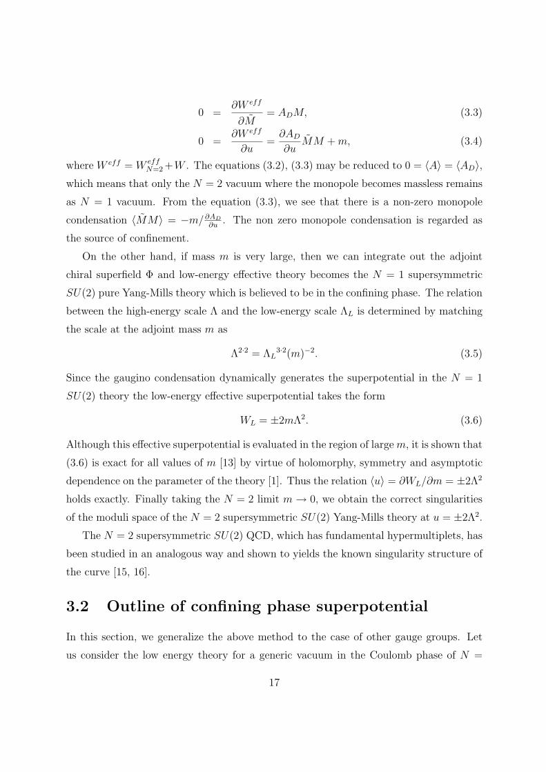
∂M= ADM, (3.3)

0 =∂W eff

∂u=

∂AD

∂uMM + m, (3.4)

where W eff = W effN=2 +W . The equations (3.2), (3.3) may be reduced to 0 = ⟨A⟩ = ⟨AD⟩,

which means that only the N = 2 vacuum where the monopole becomes massless remains

as N = 1 vacuum. From the equation (3.3), we see that there is a non-zero monopole

condensation ⟨MM⟩ = −m/∂AD

∂u. The non zero monopole condensation is regarded as

the source of confinement.

On the other hand, if mass m is very large, then we can integrate out the adjoint

chiral superfield Φ and low-energy effective theory becomes the N = 1 supersymmetric

SU(2) pure Yang-Mills theory which is believed to be in the confining phase. The relation

between the high-energy scale Λ and the low-energy scale ΛL is determined by matching

the scale at the adjoint mass m as

Λ2·2 = ΛL3·2(m)−2. (3.5)

Since the gaugino condensation dynamically generates the superpotential in the N = 1

SU(2) theory the low-energy effective superpotential takes the form

WL = ±2mΛ2. (3.6)

Although this effective superpotential is evaluated in the region of large m, it is shown that

(3.6) is exact for all values of m [13] by virtue of holomorphy, symmetry and asymptotic

dependence on the parameter of the theory [1]. Thus the relation ⟨u⟩ = ∂WL/∂m = ±2Λ2

holds exactly. Finally taking the N = 2 limit m → 0, we obtain the correct singularities

of the moduli space of the N = 2 supersymmetric SU(2) Yang-Mills theory at u = ±2Λ2.

The N = 2 supersymmetric SU(2) QCD, which has fundamental hypermultiplets, has

been studied in an analogous way and shown to yields the known singularity structure of

the curve [15, 16].

3.2 Outline of confining phase superpotential

In this section, we generalize the above method to the case of other gauge groups. Let

us consider the low energy theory for a generic vacuum in the Coulomb phase of N =

17

2 supersymmetric gauge theory with the gauge group G. Generically the low energy

behavior of this theory is described by N = 2 supersymmetric U(1)rankG pure Yang-Mills

theory. As in the previous section, we add a tree level superpotential W =∑

k gkuk,

where uk are the Casimirs built out of the adjoint chiral superfield Φ, to this N = 2

theory. According to the technique called the confining phase superpotential [18], we

concentrate on investigating the vicinity of a singular point of the N = 2 moduli space of

vacua where a single monopole or dyon becomes massless. The low energy N = 1 theory

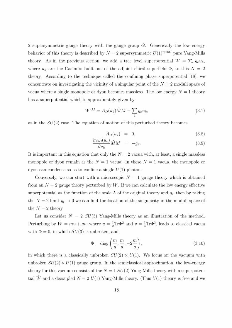
has a superpotential which is approximately given by

W eff = AD(uk)MM +∑k

gkuk, (3.7)

as in the SU(2) case. The equation of motion of this perturbed theory becomes

AD(uk) = 0, (3.8)

∂AD(uk)

∂uk

MM = −gk. (3.9)

It is important in this equation that only the N = 2 vacua with, at least, a single massless

monopole or dyon remain as the N = 1 vacua. In these N = 1 vacua, the monopole or

dyon can condense so as to confine a single U(1) photon.

Conversely, we can start with a microscopic N = 1 gauge theory which is obtained

from an N = 2 gauge theory perturbed by W . If we can calculate the low energy effective

superpotential as the function of the scale Λ of the original theory and gi, then by taking

the N = 2 limit gi → 0 we can find the location of the singularity in the moduli space of

the N = 2 theory.

Let us consider N = 2 SU(3) Yang-Mills theory as an illustration of the method.

Perturbing by W = mu + gv, where u = 12TrΦ2 and v = 1

3TrΦ3, leads to classical vacua

with Φ = 0, in which SU(3) is unbroken, and

Φ = diag

(m

g,m

g,−2

m

g

), (3.10)

in which there is a classically unbroken SU(2) × U(1). We focus on the vacuum with

unbroken SU(2)×U(1) gauge group. In the semiclassical approximation, the low-energy

theory for this vacuum consists of the N = 1 SU(2) Yang-Mills theory with a superpoten-

tial W and a decoupled N = 2 U(1) Yang-Mills theory. (This U(1) theory is free and we

18

can ignore it in the following consideration.) The scale Λ of this SU(2) theory is related

to the high-energy SU(3) scale Λ by

Λ2·2 =

(3m

g

)−2

Λ2·3, (3.11)

which is obtained by matching the SU(3) scale to the SU(2) scale at the scale (m/g) −(−2m/g) = (3m/g) of the W bosons which become massive by the Higgs effect. The

superpotential W may be evaluated as

W =1

2W ′′(m/g) TrΦ2

SU(2)+1

3 · 2W ′′′(m/g) TrΦ3

SU(2) =3m

2TrΦ2

SU(2)+g

3TrΦ3

SU(2), (3.12)

where W (x) = m2x2 + g

3x3 and ΦSU(2) is an unbroken SU(2) part of Φ. Note that in W

we suppress the terms which are not relevant to the SU(2) theory. Therefore the adjoint

chiral superfield ΦSU(2) has a mass 3m and can be integrated out. We are then left with

an N = 1 SU(2) pure Yang-Mills theory with a scale ΛL which is related to the scale Λ

by

Λ3·2L = (3m)2Λ2·2 = g2Λ6. (3.13)

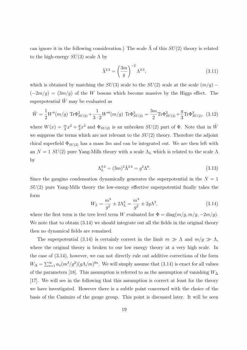
Since the gaugino condensation dynamically generates the superpotential in the N = 1

SU(2) pure Yang-Mills theory the low-energy effective superpotential finally takes the

form

WL =m3

g2± 2Λ3

L =m3

g2± 2gΛ3, (3.14)

where the first term is the tree level term W evaluated for Φ = diag(m/g,m/g,−2m/g).

We note that to obtain (3.14) we should integrate out all the fields in the original theory

then no dynamical fields are remained.

The superpotential (3.14) is certainly correct in the limit m ≫ Λ and m/g ≫ Λ,

where the original theory is broken to our low energy theory at a very high scale. In

the case of (3.14), however, we can not directly rule out additive corrections of the form

W∆ =∑∞

n=1 an(m3/g2)(gΛ/m)6n. We will simply assume that (3.14) is exact for all values

of the parameters [18]. This assumption is referred to as the assumption of vanishing W∆

[17]. We will see in the following that this assumption is correct at least for the theory

we have investigated. However there is a subtle point concerned with the choice of the

basis of the Casimirs of the gauge group. This point is discussed later. It will be seen

19

also that the statement that W∆ = 0 seems to reflect the absence of mixing of various

classical vacua like θ vacua in QCD.

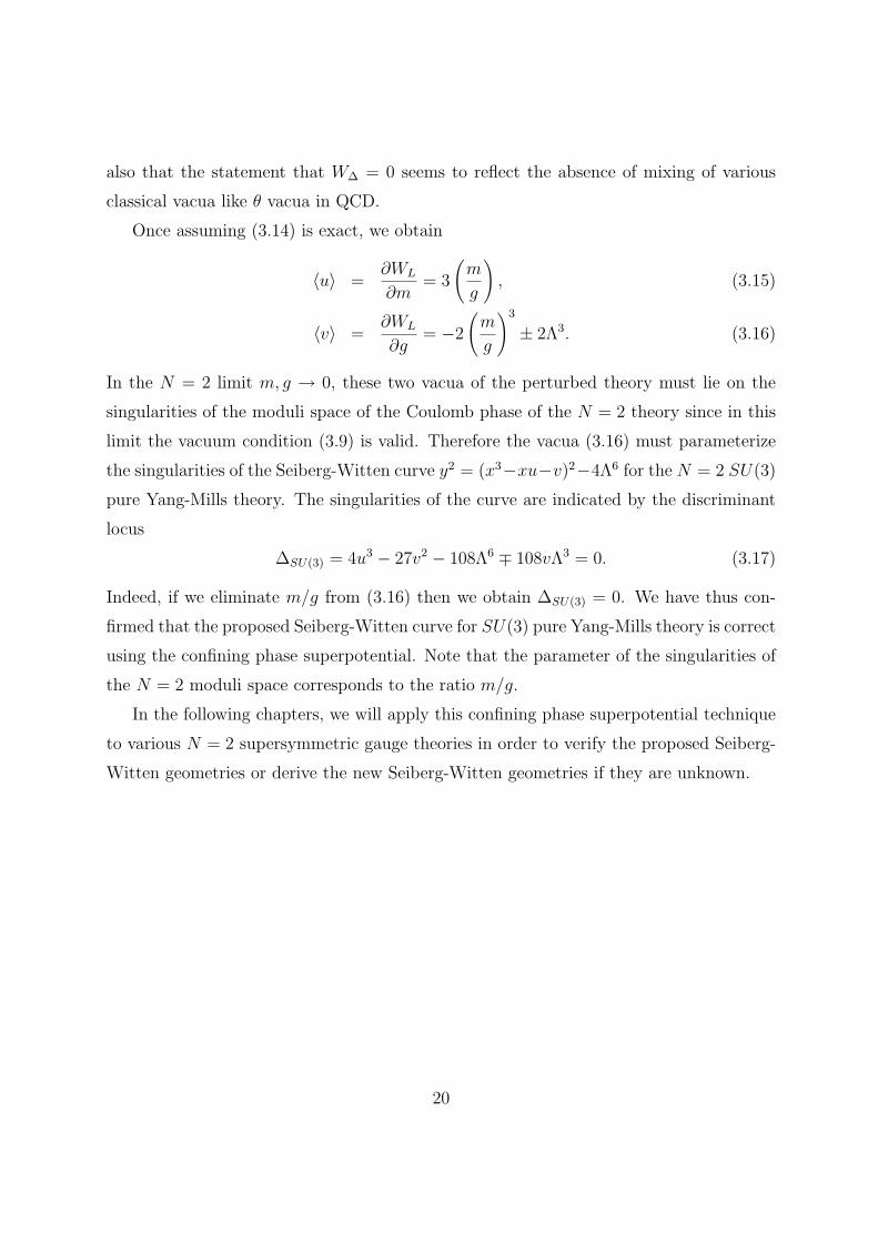
Once assuming (3.14) is exact, we obtain

⟨u⟩ =∂WL

∂m= 3

(m

g

), (3.15)

⟨v⟩ =∂WL

∂g= −2

(m

g

)3

± 2Λ3. (3.16)

In the N = 2 limit m, g → 0, these two vacua of the perturbed theory must lie on the

singularities of the moduli space of the Coulomb phase of the N = 2 theory since in this

limit the vacuum condition (3.9) is valid. Therefore the vacua (3.16) must parameterize

the singularities of the Seiberg-Witten curve y2 = (x3−xu−v)2−4Λ6 for the N = 2 SU(3)

pure Yang-Mills theory. The singularities of the curve are indicated by the discriminant

locus

∆SU(3) = 4u3 − 27v2 − 108Λ6 ∓ 108vΛ3 = 0. (3.17)

Indeed, if we eliminate m/g from (3.16) then we obtain ∆SU(3) = 0. We have thus con-

firmed that the proposed Seiberg-Witten curve for SU(3) pure Yang-Mills theory is correct

using the confining phase superpotential. Note that the parameter of the singularities of

the N = 2 moduli space corresponds to the ratio m/g.

In the following chapters, we will apply this confining phase superpotential technique

to various N = 2 supersymmetric gauge theories in order to verify the proposed Seiberg-

Witten geometries or derive the new Seiberg-Witten geometries if they are unknown.

20

Chapter 4

N = 2 Pure Yang-Mills Theory

4.1 Classical gauge groups

Now we apply the confining phase superpotential method to N = 2 supersymmetric pure

Yang-Mills theories with classical gauge groups.

First we begin with the SU(Nc) gauge theory [18]. The gauge symmetry breaks

down to U(1)Nc−1 in the Coulomb phase of N = 2 SU(Nc) Yang-Mills theories. Near

the singularity of a single massless dyon we have a photon coupled to the light dyon

hypermultiplet while the photons for the rest U(1)Nc−2 factors remain free. We now

perturb the theory by adding a tree-level superpotential

W =Nc∑

n=1

gnun, un =1

nTr Φn, (4.1)

where Φ is the adjoint N = 1 superfield in the N = 2 vectormultiplet and g1 is an auxiliary

field implementing Tr Φ = 0. In view of the macroscopic theory, we see that under the

perturbation by (4.1) only the N = 2 singular loci survive as the N = 1 vacua where a

single photon is confined and the U(1)Nc−2 factors decouple.

The result should be directly recovered when we start with the microscopic N = 1

SU(Nc) gauge theory which is obtained from N = 2 SU(Nc) Yang-Mills theory perturbed

by (4.1). For this we study the vacuum with unbroken SU(2) × U(1)Nc−2. The classical

vacua of the theory are determined by the equation of motion W ′(Φ) =∑Nc

i=1 giΦi−1 = 0.

Then the roots ai of

W ′(x) =Nc∑i=1

gixi−1 = gNc

Nc−1∏i=1

(x − ai) (4.2)

21

give the eigenvalues of Φ. In particular the unbroken SU(2) × U(1)Nc−2 vacuum is de-

scribed by

Φ = diag(a1, a1, a2, a3, · · · , aNc−1). (4.3)

In the low-energy limit the adjoint superfield for SU(2) becomes massive and will be

decoupled. We are then left with an N = 1 SU(2) Yang-Mills theory which is in the

confining phase and the photon multiplets for U(1)Nc−2 are decoupled.

The relation between the high-energy SU(Nc) scale Λ and the low-energy SU(2) scale

ΛL is determined by first matching at the scale of SU(Nc)/SU(2) W bosons and then by

matching at the SU(2) adjoint mass Mad. One finds [40], [18]

Λ2Nc = ΛL3·2

(Nc−1∏i=2

(a1 − ai)

)2

(Mad)−2. (4.4)

To compute Mad we decompose

Φ = Φcl + δΦ + δΦ, (4.5)

where δΦ denotes the fluctuation along the unbroken SU(2) direction and δΦ along the

other directions. Substituting this into W we have

W = Wcl +Nc∑i=2

gii − 1

2Tr (δΦ2Φi−2

cl ) + · · ·

= Wcl +1

2W ′′(a1) Tr δΦ2 + · · ·

= Wcl +1

2gNc

Nc∏i=2

(a1 − ai) Tr δΦ2 + · · · , (4.6)

where [δΦ, Φcl] = 0 has been used and Wcl is the tree-level superpotential evaluated in

the classical vacuum. Hence, Mad = gNc

∏Nc−1i=2 (a1 − ai) and the relation (4.4) reduces to

ΛL6 = g2

NcΛ2Nc . (4.7)

Since the gaugino condensation dynamically generates the superpotential in the N = 1

SU(2) theory the low-energy effective superpotential finally takes the form [18]

WL = Wcl ± 2ΛL3 = Wcl ± 2gNcΛ

Nc . (4.8)

22

We simply assume here that the superpotential (4.8) is exact for any values of the

parameters. (This is equivalent to assume W∆ = 0 [17], [18].) From (4.8) we obtain

⟨un⟩ =∂WL

∂gn

= ucln (g) ± 2ΛNcδn,Nc (4.9)

with ucln being a classical value of un. As we argued above these vacua should correspond

to the singular loci of N = 2 massless dyons. This can be easily confirmed by plugging

(4.9) in the N = 2 SU(Nc) curve [6], [5]

y2 = ⟨det(x − Φ)⟩2 − 4Λ2Nc =

(xNc −

Nc∑i=2

⟨si⟩xNc−i

)2

− 4Λ2Nc , (4.10)

where

ksk +k∑

i=1

isk−iui = 0, k = 1, 2, · · · (4.11)

with s0 = −1 and s1 = u1 = 0. We have

y2 =(xNc − scl

2 xNc−2 − · · · − sclNc

) (xNc − scl

2 xNc−2 − · · · − sclNc

± 4ΛNc

)= (x − a1)

2(x − a2) · · · (x − aNc−1)((x − a1)

2 · · · (x − aNc−1) ± 4ΛNc

). (4.12)

Since the curve exhibits the quadratic degeneracy we are exactly at the singular point of

a massless dyon in the N = 2 SU(Nc) Yang-Mills vacuum.

Let us now apply our procedure to the N = 2 SO(2Nc) Yang-Mills theory. We take a

tree-level superpotential to break N = 2 to N = 1 as

W =Nc−1∑n=1

g2nu2n + λv, (4.13)

where

u2n =1

2nTr Φ2n,

v = Pf Φ =1

2NcNc!ϵi1i2j1j2···Φ

i1i2Φj1j2 · · · (4.14)

and the adjoint superfield Φ is an antisymmetric 2Nc × 2Nc tensor. This theory has

classical vacua which satisfy the condition

W ′(Φ) =Nc−1∑i=1

g2i(Φ2i−1)ij −

λ

2Nc(Nc − 1)!ϵ i j k1k2l1l2···Φ

k1k2Φl1l2 · · · = 0. (4.15)

23

For the skew-diagonal form of Φ

Φ = diag(σ2e0, σ2e1, σ2e2, · · · , σ2eNc−1), σ2 = i

(0 −11 0

)(4.16)

the vacuum condition (4.15) becomes

Nc−1∑i=1

g2i(−1)i−1en2i−1 + (−i)Nc

λ

2en

Nc−1∏i=0

ei = 0 , 0 ≤ n ≤ Nc − 1. (4.17)

Thus we see that en (= 0) are the roots of f(x) defined by

f(x) =Nc−1∑i=1

g2ix2i + d, (4.18)

where we put d = (−i)Nc 12λ

∏Nc−1i=0 ei.

Since our main concern is the vacuum with a single confined photon we focus on the

unbroken SU(2) × U(1)Nc−1 vacuum. Thus writing (4.18) as

f(x) = g2(Nc−1)

Nc−1∏i=1

(x2 − a2i ), (4.19)

we take

Φ = diag(σ2a1, σ2a1, σ2a2, · · · , σ2aNc−1) (4.20)

with d = (−i)Nc 12λa2

1

∏Nc−1i=2 ai. We then make the scale matching between the high-energy

SO(2Nc) scale Λ and the low-energy SU(2) scale ΛL. Following the steps as in the SU(Nc)

case yields

Λ2·2(Nc−1) = ΛL3·2

(Nc−1∏i=2

(a21 − a2

i )

)2

(Mad)−2, (4.21)

where the factor arising through the Higgs mechanism is easily calculated in an explicit

basis of SO(2Nc). In order to evaluate the SU(2) adjoint mass Mad we first substitute

the decomposition (4.5) in W and proceed as follows:

W = Wcl +Nc−1∑i=1

gi2i − 1

2Tr (δΦ2Φ2i−2

cl ) + λ (Pf4δΦ)(Pf2(Nc−2)Φcl

)+ · · ·

= Wcl +Nc−1∑i=1

gi2i − 1

2Tr (δΦ2Φ2i−2

cl ) + λ(

1

4Tr δΦ2

) (Nc−1∏k=2

(−iak)

)+ · · ·

= Wcl +1

2

d

dx

(f(x)

x

)∣∣∣∣∣x=a1

Tr δΦ2 + · · ·

= Wcl + g2(Nc−1)

Nc−1∏i=2

(a21 − a2

i ) Tr δΦ2 + · · · , (4.22)

24

where Pf4 is the Pfaffian of a upper-left 4 × 4 sub-matrix and Pf2(Nc−2) is the Pfaffian

of a lower-right 2(Nc − 2) × 2(Nc − 2) sub-matrix. Thus we observe that Mad cancels

out the Higgs factor in (4.21), which leads to ΛL6 = g2

2(Nc−1)Λ4(Nc−1). The low-energy

superpotential is now given by

WL = Wcl ± 2ΛL3 = Wcl ± 2g2(Nc−1)Λ

2(Nc−1), (4.23)

where the second term is due to the gaugino condensation in the low-energy SU(2) theory.

The vacuum expectation values of gauge invariants are obtained from WL as

⟨u2n⟩ =∂WL

∂g2n

= ucl2n(g, λ) ± 2Λ2(Nc−1)δn,Nc−1,

⟨v⟩ =∂WL

∂λ= vcl(g, λ). (4.24)

The curve for N = 2 SO(2Nc) is known to be [8]

y2 = ⟨det(x − Φ)⟩2 − 4Λ4(Nc−1)x4

=(x2Nc −

Nc−1∑i=1

⟨s2i⟩x2(Nc−i) + ⟨v⟩2)2

− 4Λ4(Nc−1)x4, (4.25)

where

ksk +k∑

i=1

isk−iu2i = 0, k = 1, 2, · · · (4.26)

with s0 = −1. At the values (4.24) of the moduli coordinates we see the quadratic

degeneracy

y2 =(x2Nc − scl

2 x2(Nc−1) − · · · − scl2(Nc−1)x

2 + v2cl

)×

(x2Nc − scl

2 x2(Nc−1) − · · · − scl2(Nc−1)x

2 + v2cl ± 4Λ2(Nc−1)x2

)= (x2 − a2

1)2(x2 − a2

2) · · · (x2 − a2Nc−1)

×((x2 − a2

1)2(x2 − a2

2) · · · (x2 − a2Nc−1) ± 4Λ2(Nc−1)x2

). (4.27)

This is our desired result. Notice that the apparent singularity at ⟨v⟩ = 0 is not realized

in our N = 1 theory. Thus the point ⟨v⟩ = 0 does not correspond to massless solitons in

agreement with the result of [8].

25

Our next task is to study the SO(2Nc + 1) gauge theory. A tree-level superpotential

breaking N = 2 to N = 1 is assumed to be

W =Nc∑

n=1

g2nu2n, u2n =1

2nTr Φ2n. (4.28)

The classical vacua obey W ′(Φ) =∑Nc

i=1 g2iΦ2i−1 = 0. The eigenvalues of Φ are given by

the roots ai of

W ′(x) =Nc∑i=1

g2ix2i−1 = g2Ncx

Nc−1∏i=1

(x2 − a2i ). (4.29)

As in the previous consideration we take the SU(2) × U(1)Nc−1 vacuum. Notice that

there are two ways of breaking SO(2Nc + 1) to SU(2) × U(1)Nc−1. One is to take all

the eigenvalues distinct (corresponding to SO(3) × U(1)Nc−1). The other is to choose

two eigenvalues coinciding and the rest distinct (corresponding to SU(2)×U(1)Nc−1 with

ai = 0). Here we examine the latter case

Φ = diag(σ2a1, σ2a1, σ2a2, · · · , σ2aNc−1, 0), σ2 = i

(0 −11 0

). (4.30)

In this vacuum the high-energy SO(2Nc + 1) scale Λ and the low-energy SU(2) scale ΛL

are related by

Λ2·(2Nc−1) = ΛL3·2a2

1

(Nc−1∏i=2

(a21 − a2

i )

)2

(Mad)−2, (4.31)

where the SU(2) adjoint mass Mad is read off from

W = Wcl +Nc∑i=1

g2i2i − 1

2Tr (δΦ2Φ2i−2

cl ) + · · ·

= Wcl +1

2W ′′(a1) Tr δΦ2 + · · ·

= Wcl + g2Nca21

Nc−1∏i=2

(a21 − a2

i ) Tr δΦ2 + · · · . (4.32)

So, we obtain ΛL6 = g2

2Nca2

1Λ2(2Nc−1). The low-energy effective superpotential becomes

WL = Wcl ± 2ΛL3 = Wcl ± 2g2Nca1Λ

2Nc−1. (4.33)

If we assume W∆ = 0 the expectation values ⟨u2i⟩ are calculated from WL by expressing

a1 as a function of g2i.

26

For the sake of illustration let us discuss the SO(5) theory explicitly. From (4.33) we

get

⟨u2⟩ = 2a21 ±

1

a1

Λ3,

⟨u4⟩ = a41 ∓ a1Λ

3 (4.34)

and a21 = −g2/g4. We eliminate a1 from (4.34) to obtain

27Λ12 − Λ6u32 + 36Λ6u2u4 − u4

2u4 + 8u22u

24 − 16u3

4 = 0. (4.35)

This should be compared with the N = 2 SO(5) discriminant [7]

s22(27Λ12 − Λ6s3

1 − 36Λ6s1s2 + s41s2 + 8s2

1s22 + 16s3

2)2 = 0, (4.36)

where s1 = u2 and s2 = u4 − u22/2 according to (4.26). Thus we see the discrepancy

between (4.35) and (4.36) which implies that our simple assumption of W∆ = 0 does

not work. Inspecting (4.35) and (4.36), however, we notice how to remedy the difficulty.

Instead of (4.28) we take a tree-level superpotential

W = g2s1 + g4s2 = g2u2 + g4

(u4 −

1

2u2

2

). (4.37)

The classical vacuum condition is

W ′(Φ) = (g2 − g4u2)Φ + g4Φ3 = 0. (4.38)

To proceed, therefore, we can make use of the results obtained in the foregoing analysis

just by making the replacement

g4 → g4 = g4,

g2 → g2 = g2 − u2g4. (4.39)

(especially evaluation of Mad is not invalidated because Tr δΦ = 0.) The eigenvalues of Φ

are now determined in a self-consistent manner by

W ′(x) = g2x + g4x3 = g4x

(x2 +

g2

g4

)= g4x(x2 − a2

1) = 0. (4.40)

27

Then we have ucl2 = 2a2

1 = −2g2/g4 and g2 = −g2 from (4.39), which leads to

a21 =

g2

g4

. (4.41)

Substituting this in (4.33) we calculate ⟨si⟩ and find the relation of si which is precisely

the discriminant (4.36) except for the classical singularity at ⟨s2⟩ = 0.

The above SO(5) result indicates that an appropriate mixing term with respect to u2i

variables in a microscopic superpotential will be required for SO(2Nc + 1) theories. We

are led to assume

W =Nc−1∑i=1

g2iu2i + g2NcsNc (4.42)

for the gauge group SO(2Nc + 1) with Nc ≥ 3. Then the following analysis is analogous

to the SO(5) theory. First of all notice that

sNc = u2Nc − u2(Nc−1)u2 + (polynomials of u2k, 1 ≤ k < Nc − 1). (4.43)

Therefore the eigenvalues of Φ are given by the roots of (4.29) with the replacement

g2Nc → g2Nc = g2Nc ,

g2(Nc−1) → g2(Nc−1) = g2(Nc−1) − u2g2Nc . (4.44)

Then we have u2 = a21 +

∑Nc−1k=1 a2

k = a21 − g2(Nc−1)/g2Nc and find

a21 =

g2(Nc−1)

g2Nc

. (4.45)

It follows that the effective superpotential is given by

WL = W clL ± 2

√g2Ncg2(Nc−1)Λ

2Nc−1. (4.46)

The vacuum expectation values of gauge invariants are obtained from WL as

⟨sn⟩ = scln (g), 1 ≤ n ≤ Nc − 2

⟨sNc−1⟩ = sclNc−1(g) ± 1

a1

Λ2Nc−1,

⟨sNc⟩ = sclNc

(g) ± a1Λ2Nc−1. (4.47)

28

For these ⟨si⟩ the curve describing the N = 2 SO(2Nc + 1) theory [7] is shown to be

degenerate as follows:

y2 = ⟨det(x − Φ)⟩2 − 4x2Λ2(2Nc−1)

= (x2Nc − ⟨s1⟩x2(Nc−1) − · · · − ⟨sNc−1⟩x2 − ⟨sNc⟩ + 2xΛ2Nc−1)

×(x2Nc − ⟨s1⟩x2(Nc−1) − · · · − ⟨sNc−1⟩x2 − ⟨sNc⟩ − 2xΛ2Nc−1)

=

(x2 − a2

1)2(x2 − a2

2) · · · (x2 − a2Nc−1) ± Λ2Nc−1

(−x2

a1

− a1 + 2x

)

×

(x2 − a21)

2(x2 − a22) · · · (x2 − a2

Nc−1) ± Λ2Nc−1

(−x2

a1

− a1 − 2x

)

= (x2 − a21)

2

((x + a1)

2(x2 − a22) · · · (x2 − a2

Nc−1) ∓Λ2Nc−1

a1

)

×(

(x − a1)2(x2 − a2

2) · · · (x2 − a2Nc−1) ∓

Λ2Nc−1

a1

). (4.48)

Thus we see the theory with the superpotential (4.42) recover the N = 2 curve correctly

with the assumption W∆ = 0. As in the SO(2Nc) case, the singularity at ⟨sNc⟩ = 0, which

corresponds to the classical SO(3) × U(1)Nc−1 vacuum, does not arise in our theory.

We remark that the particular form of superpotential (4.42) is not unique to derive

the singularity manifold. In fact we may start with a superpotential

W =Nc−1∑i=1

g2i (u2i + hi(s)) + g2Nc (sNc + hNc(s)) , (4.49)

where hi(s) are arbitrary polynomials of sj with j ≥ Nc − 2, to verify the N = 2 curve.

However, we are not allowed to take a superpotential such as W =∑Nc

i=1 g2isi, because

there are no SU(2) × U(1)Nc−1 vacua (there exist no solutions for g2(Nc−1)). Note also

that there are no SO(3) × U(1)Nc−1 vacua in the theory with superpotential (4.49).

Finally we discuss the Sp(2Nc) gauge theory. The adjoint superfield Φ is a 2Nc × 2Nc

tensor which is subject to

tΦ = JΦJ ⇐⇒ JΦ is symmetric, (4.50)

where J = diag(iσ2, · · · , iσ2). Let us assume a tree-level superpotential

W =Nc∑

n=1

g2nu2n, u2n =1

2nTr Φ2n. (4.51)

29

Then our analysis will become quite similar to that for SO(2Nc+1). The classical vacuum

with unbroken SU(2) × U(1)Nc−1 gauge group corresponds to

JΦ = diag(σ1a1, σ1a1, σ1a2, · · · , σ1aNc−1), σ1 =

(0 11 0

). (4.52)

The scale matching relation becomes

Λ2·(Nc+1) = ΛL3·2· 1

2 a41

(Nc−1∏i=2

(a21 − a2

i )

)2

(Mad)−1. (4.53)

Since the SU(2) adjoint mass is given by Mad = g2Nca21

∏Nc−1i=2 (a2

1 − a2i ) we get ΛL

3 =

g2NcΛ2(Nc+1)/a2

1. The low-energy effective superpotential thus turns out to be

WL = Wcl + 2g2Nc

a21

Λ2(Nc+1). (4.54)

Checking the result with Sp(4) we encounter the same problem as in the SO(5) theory.

Instead of (4.51), thus, we take a superpotential in the form (4.37), reproducing the N = 2

Sp(4) curve [11]. Similarly, for Sp(2Nc) we study a superpotential (4.42). It turns out

that ⟨si⟩ are calculated as

⟨sn⟩ = scln (g), 1 ≤ n ≤ Nc − 2,

⟨sNc−1⟩ = sclNc−1(g) − 2

a41

Λ2(Nc+1),

⟨sNc⟩ = sclNc

(g) +4

a21

Λ2(Nc+1). (4.55)

These satisfy the N = 2 Sp(2Nc) singularity condition [11] since the curve exhibits the

quadratic degeneracy

x2y2 =(x2 ⟨det(x − Φ)⟩ + Λ2(Nc+1)

)2− Λ4(Nc+1)

= (x2(Nc+1) − ⟨s1⟩x2Nc − · · · − ⟨sNc−1⟩x4 − ⟨sNc⟩x2 + 2Λ2(Nc+1))

×(x2(Nc+1) − ⟨s1⟩x2Nc − · · · − ⟨sNc−1⟩x4 − ⟨sNc⟩x2)

=

x2(x2 − a2

1)2(x2 − a2

2) · · · (x2 − a2Nc−1) + 2Λ2(Nc+1)

((x

a1

)4

− 2(

x

a1

)2

+ 1

)×

(x2det(x − Φcl)

)= (x2 − a2

1)2

(x2(x2 − a2

2) · · · (x2 − a2Nc−1) +

Λ2(Nc+1)

a41

)×

(x2det(x − Φcl)

). (4.56)

It should be mentioned that our remarks on SO(2Nc + 1) theories also apply here.

30

4.2 ADE gauge groups

Our purpose in this section is to show that, under an appropriate ansatz, the low-energy

effective superpotential for the Coulomb phase is obtained in a unified way for all ADE

gauge groups just by using the fundamental properties of the root system ∆. Let us

consider the case of the gauge group G is simple and simply-laced, namely, G is of ADE

type. Our notation for the root system is as follows. The simple roots of G are denoted as

αi where 1 ≤ i ≤ r with r being the rank of G. Any root is decomposed as α =∑r

i=1 aiαi.

The component indices are lowered by ai =∑r

j=1 Aijaj where Aij is the ADE Cartan

matrix. The inner product of two roots α, β are then defined by

α · β =r∑

i=1

aibi =r∑

i,j=1

aiAijbj, (4.57)

where β =∑r

i=1 biαi. For ADE all roots have the equal norm and we normalize α2 = 2.

In our N = 1 theory we take a tree-level superpotential

W =r∑

k=1

gkuk(Φ), (4.58)

where uk is the k-th Casimir of G constructed from Φ and gk are coupling constants. The

mass dimension of uk is ek + 1 with ek being the k-th exponent of G. When gk = 0 Φ

is considered as the chiral field in the N = 2 vector multiplet and we have N = 2 ADE

supersymmetric gauge theory.

We first make a classical analysis of the theory with the superpotential (4.58). The

classical vacua are determined by the equation of motion ∂W∂Φ

= 0 and the D-term equation.

Due to the D-term equation, we can restrict Φ to take the values in the Cartan subalgebra

by the gauge rotation. We denote the vector in the Cartan subalgebra corresponding to

the classical value of Φ as a =∑r

i=1 aiαi. Then the superpotential becomes

W (a) =r∑

k=1

gkuk(a), (4.59)

and the equation of motion reads

∂W (a)

∂ai=

r∑k=1

gk∂uk(a)

∂ai= 0. (4.60)

31

For gk ≡ 0 we must have

J(a) ≡ det

(∂uj(a)

∂ai

)= 0. (4.61)

According to [41] it follows that

J(a) = c1

∏α∈∆+

a · α, (4.62)

where ∆+ is a set of positive roots and c1 is a certain constant.

The condition J(a) = 0 means that the vector a hits a wall of the Weyl chamber and

there occurs enhanced gauge symmetry. Suppose that the vector a is orthogonal to a

root, say, α1

a · α1 = 0, (4.63)

where α1 may be taken to be a simple root. In this case we have the unbroken gauge

group SU(2) × U(1)r−1 where the SU(2) factor is spanned by α1 · H,Eα1 , E−α1 in the

Cartan-Weyl basis. If some other factors of J vanish besides a · α1 the gauge group is

further enhanced from SU(2). Since SU(2)×U(1)r−1 is the most generic unbroken gauge

group we shall restrict ourselves to this case in what follows.

We remark here that there is the case in which the SU(2) × U(1)r−1 vacuum is not

generic. As a simple, but instructive example consider SU(4) theory. Casimirs are taken

to be

u1 =1

2Tr Φ2,

u2 =1

3Tr Φ3,

u3 =1

4Tr Φ4 − α

(1

2Tr Φ2

)2

, (4.64)

where α is an arbitrary constant. If we set α = 1/2 it is observed that the SU(2)×U(1)2

vacuum exists only for the special values of coupling constants, (g2/g3)2 = g1/g3. Thus,

for α = 1/2, the SU(2)×U(1)2 vacuum is not generic though it does so for α = 1/2. This

points out that we have to choose the appropriate basis for Casimirs when writing down

(4.58) to have the SU(2) × U(1)r−1 vacuum generically [19].

Now we assume that there is no mixing between the SU(2) × U(1)r−1 vacuum and

other vacua with different unbroken gauge groups. According to the arguments of [49], we

32

should not consider the broken gauge group instantons. We thus expect that there is only

perturbative effect in the energy scale above the scale ΛY M of the low-energy effective

N = 1 supersymmetric SU(2) Yang-Mills theory.

Our next task is to evaluate the Higgs scale associated with the spontaneous breaking

of the gauge group G to SU(2) × U(1)r−1. For this purpose we decompose the adjoint

representation of G to irreducible representations of SU(2). We fix the SU(2) direction

by taking a simple root α1. It is clear that the spin j of every representation obtained

in this decomposition satisfies j ≤ 1 since all roots have the same norm and the SU(2)

raising (or lowering) operator shifts a root α to α + α1 (or α − α1). The fact that there

is no degeneration of roots indicates that the j = 1 multiplet has the roots (α1, 0,−α1)

corresponding to the unbroken SU(2) generators. The roots orthogonal to α1 represent

the j = 0 multiplets. The j = 1/2 multiplets have the roots α obeying α · α1 = ±1. Let

us define a set of these roots by ∆d = α|α ∈ ∆, α · α1 = ±1. For each root α ∈ ∆d

there appears a massive gauge boson. These massive bosons pair up in SU(2) doublets

with weights (α, α ± α1) which indeed have the same mass |a · α| = |a · (α ± α1)| since

a · α1 = 0.

We now integrate out the fields that become massive by the Higgs mechanism. The

massless U(1)r−1 degrees of freedom are decoupled. The resulting theory characterized

by the scale ΛH is N = 1 SU(2) theory with an adjoint chiral multiplet. The Higgs scale

ΛH is related to the high-energy scale Λ through the scale matching relation

Λ2h = Λ2·2H

∏β∈∆d, β>0

a · β

ℓ

, (4.65)

where 2h = 4 + ℓnd/2, nd is the number of elements in ∆d and h stands for the dual

Coxeter number of G; h = r + 1, 2r − 2, 12, 18, 30 for G = Ar, Dr, E6, E7, E8 respectively.

The reason for β > 0 in (4.65) is that weights (β, β ± α1) of an SU(2) doublet are either

both positive or both negative since α1 is the simple root, and gauge bosons associated

with β < 0 and β > 0 have the same contribution to the relation (4.65).

To fix ℓ we calculate nd by evaluating the quadratic Casimir C2 of the adjoint repre-

sentation in the following way. Taking hermitian generators we express C2 in terms of the

structure constants fabc through∑

a,b fabcfabc′ = −C2 δcc′ . From the commutation relation

33

[α1 · H,Eα] = (α1 · α)Eα one can check

C2 =1

2

∑α∈∆

(α1 · α)2 =1

2

∑α∈∆d

(α1 · α)2 + 2(α1 · α1)2

=1

2(nd + 8) . (4.66)

On the other hand, the dual Coxeter number h is given by h = C2/θ2 with θ being the

highest root. We thus find

nd = 4(h − 2) (4.67)

and (4.65) becomes

Λ2h = Λ2·2H

∏β∈∆d, β>0

a · β. (4.68)

After integrating out the massive fields due to the Higgs mechanism we are left with

N = 1 SU(2) theory with the massive adjoint. In order to evaluate the mass of the adjoint

chiral multiplet Φ we need to clarify some properties of Casimirs. Let σβ be an element

of the Weyl group of G specified by a root β =∑r

i=1 biαi. The Weyl transformation of a

root α is given by

σβ(α) = α − (α · β)β. (4.69)

When σβ acts on the Higgs v.e.v. vector a =∑r

i=1 aiαi we have

a′i =r∑

j=1

Sβij aj, Sβ

ij ≡ δi

j − bibj, (4.70)

where σβ(a) =∑r

i=1 a′iαi. Since the Casimirs uk(a) are Weyl invariants it is obvious to

see∂

∂aiuk(a) =

∂

∂aiuk(a

′) =r∑

j=1

Sβji

(∂

∂ajuk(a)

)∣∣∣∣∣a→a′

. (4.71)

Let a be a particular v.e.v. which is fixed under the action of σβ, then we find the identity

r∑j=1

(δj

i − Sβji

) ∂

∂ajuk(a)

∣∣∣∣∣∣a=a

= 0 (4.72)

for all i, and thusr∑

j=1

bj∂

∂ajuk(a)

∣∣∣∣∣∣a=a

= 0. (4.73)

This implies that for any v.e.v. vector a and root β we can write down

r∑j=1

bj ∂

∂ajuk(a) = (a · β) uβ

k(a), (4.74)

34

where uβk(a) is some polynomial of ai. If we set β = αi, a simple root, we obtain a useful

formula∂

∂aiuk(a) = ai uαi

k (a). (4.75)

As an immediate application of the above results, for instance, we point out that (4.62)

is derived from (4.74) and the fact that the mass dimension of J(a) is given by

r∑k=1

ek =1

2(dim G − r), (4.76)

where ek is the k-th exponent of G.

Let us further discuss the properties of uαj

k (a). Define Dmn as

Dmn ≡ (−1)n+mdet

(∂uj(a)

∂ai

), 1 ≤ m, n ≤ r, (4.77)

where 1 ≤ i, j ≤ r with i = m, j = n, then D1n is a homogeneous polynomial of ai with

the mass dimension∑r

k=1 ek − en. We also denote ∆e as a set of positive roots where α1

and SU(2) doublet roots α with α + α1 ∈ ∆+ are excluded. If we set a1 = 0 and a ·β = 0

where β is any root in ∆e we see D1n = 0 from the identity (4.74). Consequently we can

expand

D1n = hn(a)∏

β∈∆e

(a · β) + a1fn(a), (4.78)

where hn(a), fn(a) are polynomials of ai. In particular

D1r = c2

∏β∈∆e

(a · β) + a1fr(a), (4.79)

where c2 is a constant. Notice that the first term on the rhs has the correct mass dimension

since the number of roots in ∆e reads

1

2(dim G − r) − 1 − nd

4=

r∑k=1

ek − (h − 1), (4.80)

where we have used (4.67) and er = h − 1.

We are now ready to evaluate the mass of Φ in intermediate SU(2) theory. The

fluctuation of W (a) around the classical vacuum yields the adjoint mass. To find the

mass relevant for the scale matching we should only consider the components of Φ which

are coupled to the unbroken SU(2). The mass MΦ of these components is then given by

2MΦ =∂2

(∂a1)2W (a)

∣∣∣∣∣ =∂

∂a1(a1W1)

∣∣∣∣∣ =

(a1

∂

∂a1W1 + 2W1

)∣∣∣∣∣ = 2W1| , (4.81)

35

where W1 = (∑r

k=1 gkuα1k )(a) and ai are understood as solutions of the equation of motion

(4.60).

To proceed further it is convenient to rewrite the equation motion (4.60) and the

vacuum condition (4.63) with the simple root α1 as follows:

g1 : g2 : · · · : gr = D11 : D12 : · · · : D1r,

a1 = 0. (4.82)

The solutions of these equations are expressed as functions of the ratio gi/gr. Then we

notice that J(a) defined in (4.61) turns out to be

J =r∑

k=1

∂uk

∂a1D1k =

D1r

gr

r∑k=1

gk∂uk

∂a1= D1r a1

W1

gr

. (4.83)

Combining (4.62) and (4.79) we obtain

M2Φ = (W1|)2 =

(c1

c2

)2

g2r

∏β∈∆d, β>0

a · β. (4.84)

Upon integrating out the massive adjoint we relate the scale ΛH with the scale ΛY M

of the low-energy N = 1 SU(2) Yang-Mills theory by

Λ2·2H = Λ3·2

Y M/M2Φ. (4.85)

We finally find from this and (4.65), (4.84) that the scale matching relation becomes

Λ3·2Y M = g2

rΛ2h, (4.86)

where the top Casimir ur has been rescaled so that we can set c1/c2 = 1.

Following the previous discussions and the perturbative nonrenormalization theorem

for the superpotential, we derive the low-energy effective superpotential

WL = Wcl(g) ± 2ΛY M3 = Wcl(g) ± 2grΛ

h, (4.87)

where the term ±2ΛY M3 appears as a result of the gaugino condensation in low-energy

SU(2) theory and Wcl(g) is the tree-level superpotential evaluated at the classical values

ai(g). We will assume that (4.87) is the exact effective superpotential valid for all values

of parameters.

36

The vacuum expectation values of gauge invariants are obtained from WL

⟨uk⟩ =∂WL

∂gk

= uclk (g) ± 2Λhδk,r. (4.88)

We now wish to show that the expectation values (4.88) parametrize the singularities of

algebraic curves. For this let us introduce

PR(x, uclk ) = det(x − ΦR) (4.89)

which is the characteristic polynomial in x of order dimR where R is an irreducible

representation of G. Here ΦR is a representation matrix of R and uclk are Casimirs built

out of ΦR. The eigenvalues of ΦR are given in terms of the weights λi of the representation

R. Diagonalizing ΦR we may express (4.89) as

PR(x, a) =dimR∏i=1

(x − a · λi), (4.90)

where a is a Higgs v.e.v. vector, the discriminant of which takes the form

∆R =

∏i=j

a · (λi − λj)

2

. (4.91)

It is seen that, for a which is a solution to (4.60), we have ∆R = 0, that is

PR(x, uclk (a)) = ∂xPR(x, ucl

k (a)) = 0 (4.92)

for any representation. The solutions of the classical equation of motion thus give rise to

the singularities of the level manifold PR(x, uclk ) = 0.

In order to include the quantum effect what we should do is to modify the top Casimir

ur term so that the gluino condensation in (4.88) is properly taken into account. We are

then led to take a curve

PR(x, z, uk) ≡ PR

(x, uk + δk,r

(z +

µ

z

))= 0, (4.93)

where µ = Λ2h and an additional complex variable z has been introduced. Let us check

the degeneracy of the curve at the expectation values (4.88), which means to check if the

37

following three equations hold

PR(x, z, ⟨uk⟩) = 0, (4.94)

∂xPR(x, z, ⟨uk⟩) = 0, (4.95)

∂zPR(x, z, ⟨uk⟩) =(1 − µ

z2

)∂ur PR(x, z, ⟨uk⟩) = 0. (4.96)

The last equation (4.96) has an obvious solution z = ∓√µ. Substituting this into the first

two equations we see that the singularity conditions reduce to the classical ones (4.92)

PR(x,∓√µ, ⟨uk⟩) = PR (x, ⟨uk⟩ ∓ δk,r2

õ) = PR(x, ucl

k ) = 0, (4.97)

∂xP (x,∓√µ, ⟨uk⟩) = ∂xPR (x, ⟨uk⟩ ∓ δk,r2

√µ) = ∂xPR(x, ucl

k ) = 0. (4.98)

Thus we have shown that (4.88) parametrize the singularities of the Riemann surface

described by (4.93) irrespective of the representation R.

Let us take the N = 2 limit by letting all gi → 0 with the ratio gi/gr fixed, then (4.93)

is the curve describing the Coulomb phase of N = 2 supersymmetric Yang-Mills theory

with ADE gauge groups. Indeed the curve (4.93) in this particular form of foliation agrees

with the one obtained systematically in [23] in view of integrable systems [42],[43],[44].

For E6 and E7 see [24],[25].

Finally we remark that there is a possibility of (4.96) having another solutions besides

z = ∓√µ. If we take the fundamental representation such solutions are absent for G = Ar,

and for G = Dr there is a solution with vanishing degree r Casimir (i.e. Pfaffian), but it

is known that this is an apparent singularity [8]. For Er gauge groups there could exist

additional solutions. We expect that these singularities are apparent and do not represent

physical massless solitons.

4.2.1 N = 1 superconformal field theory

We will discuss non-trivial fixed points in our N = 1 theory characterized by the mi-

croscopic superpotential (4.58). To find critical points we rely on the construction of

N = 2 superconformal field theories realized at particular points in the moduli space of

the Coulomb phase [14],[45],[46],[47]. At these N = 2 critical points mutually non-local

massless dyons coexist. Thus the critical points lie on the singularities in the moduli

38

space which are parametrized by the N = 1 expectation values (4.88) as was shown in the

previous section. This enables us to adjust the microscopic parameters in N = 1 theory

to the values of N = 2 non-trivial fixed points. Doing so in N = 2 SU(3) Yang-Mills

theory Argyres and Douglas found non-trivial N = 1 fixed points [14]. We now show that

this class of N = 1 fixed points exists in all ADE N = 1 theories in general.

Let us start with rederiving N = 2 critical behavior based on the curve (4.93). An

advantage of using the curve (4.93) is that one can identify higher critical points and

determine the critical exponents independently of the details of the curve.

If we set z = ∓√µ the condition for higher critical points is

PR(x, uclk ) = ∂n

xPR(x, uclk ) = 0 (4.99)

with n > 2. Hence there exist higher critical points at uk = usingk ± 2Λhδk,r where using

k

are the classical values of uk for which the gauge group H with rank larger than one is

left unbroken. The highest critical point corresponding to the unbroken G is located at

uk = ±2Λhδk,r.

Near the highest critical point the curve (4.93) behaves as

ur + z +µ

z= c xh + δuk xj, (4.100)

where the second term on the rhs with j = h − (ek + 1) represents a small perturbation

around the criticality at δuk = 0. A constant c is irrelevant and will be set to c = 1. Let

ur = ±2Λh, x = δu1/(h−j)k s and z ± Λh = ρ, then (4.100) becomes

ρ ≃ δuh

2(h−j)

k (∓Λh)12 (sh + sj)

12 . (4.101)

We now apply the technique of [46] to verify the scaling behavior of the period integral of

the Seiberg-Witten differential λSW . For the curve (4.93) it is known that λSW = xdz/z.

Near the critical value z = ∓√µ we evaluate∮

λSW =∮

xdz

z≃

∮xdρ

≃ δuh+2

2(h−j)

k

∮ds

hsh + jsj

(sh + sj)1/2. (4.102)

Since the period has the mass dimension one we read off critical exponents

2 (ek + 1)

h + 2, k = 1, 2, · · · , r (4.103)

39

in agreement with the results obtained earlier for N = 2 ADE Yang-Mills theories [46],[47].

When our N = 1 theory is viewed as N = 2 theory perturbed by the tree-level

superpotential (4.58) we understand that the mass gap in N = 1 theory arises from the

dyon condensation [3]. Let us show that the dyon condensate vanishes as we approach

the N = 2 highest critical point under N = 1 perturbation. The SU(2)×U(1)r−1 vacuum

in N = 1 theory corresponds to the N = 2 vacuum where a single monopole or dyon

becomes massless. The low-energy effective superpotential takes the form

Wm =√

2AMM +r∑

k=1

gkUk, (4.104)

where A is the N = 1 chiral superfield in the N = 2 U(1) vector multiplet, M, M are

the N = 1 chiral superfields of an N = 2 dyon hypermultiplet and Uk represent the

superfields corresponding to Casimirs uk(Φ). We will use lower-case letters to denote the

lowest components of the corresponding upper-case superfields. Note that ⟨a⟩ = 0 in the

vacuum with a massless soliton.

The equation of motion dWm = 0 is given by

− gk√2

=∂A

∂Uk

MM, 1 ≤ k ≤ r (4.105)

and AM = AM = 0, from which we have

gk

gr

=∂a/∂uk

∂a/∂ur

, 1 ≤ k ≤ r − 1, (4.106)

when ⟨a⟩ = 0. The vicinity of N = 2 highest criticality may be parametrized by

⟨uk⟩ = ±2Λhδk,r + ck ϵek+1, ck = constant, (4.107)

where ϵ is an overall mass scale. From (4.102) one obtains

∂a

∂uk

≃ ϵh2−ek , 1 ≤ k ≤ r, (4.108)

so thatgk

gr

≃ ϵh−ek−1 −→ 0, 1 ≤ k ≤ r − 1 (4.109)

as ϵ → 0. The scaling behavior of dyon condensate is easily derived from (4.105)

⟨m⟩ =(− gr√

2∂a/∂ur

)1/2≃ √

gr ϵ(h−2)/4 −→ 0. (4.110)

40

Therefore the gap in the N = 1 confining phase vanishes. We thus find that N = 1 ADE

gauge theory with an adjoint matter with a tree-level superpotential

Wcrit = grur(Φ) (4.111)

exhibits non-trivial fixed points. The higher-order polynomial ur(Φ) is a dangerously

irrelevant operator which is irrelevant at the UV gaussian fixed point, but affects the

long-distance behavior significantly [40].

41

Chapter 5

N = 2 Gauge Theory with MatterMultiplets

In this chapter, we extend our analysis to describe the Coulomb phase of N = 1 supersym-

metric gauge theories with Nf flavors of chiral matter multiplets Qi, Qj (1 ≤ i, j ≤ Nf )

in addition to the adjoint matter Φ. Here Q belongs to an irreducible representation

R of the gauge group G with the dimension dR and Q belongs to the conjugate repre-

sentation of R. A tree-level superpotential consists of the Yukawa-like term QΦlQ in

addition to the Casimir terms built out of Φ, and we shall consider arbitrary classical

gauge groups and ADE gauge groups. In the appropriate limit the theory is reduced to

N = 2 supersymmetric QCD.

5.1 Classical gauge groups and fundamental matters

We start with discussing N = 1 SU(Nc) supersymmetric gauge theory with an adjoint

matter field Φ, Nf flavors of fundamentals Q and anti-fundamentals Q. We take a tree-

level superpotential

W =Nc∑

n=1

gnun +r∑

l=0

TrNfλl QΦlQ, un =

1

nTr Φn, (5.1)

where TrNfλl QΦlQ =

∑Nf

i,j=1(λl)ijQiΦ

lQj and r ≤ Nc − 1. If we set (λ0)ij = mi

j with

[m,m†] = 0, (λ1)ij = δi

j, (λl)ij = 0 for l > 1 and all gi = 0, eq.(5.1) recovers the superpo-

tential in N = 2 SU(Nc) supersymmetric QCD with quark mass m. The second term in

(5.1) was considered in a recent work [48].

42

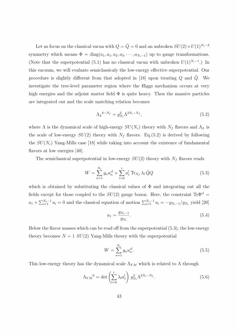
Let us focus on the classical vacua with Q = Q = 0 and an unbroken SU(2)×U(1)Nc−2

symmetry which means Φ = diag(a1, a1, a2, a3, · · · , aNc−1) up to gauge transformations.

(Note that the superpotential (5.1) has no classical vacua with unbroken U(1)Nc−1.) In

this vacuum, we will evaluate semiclassicaly the low-energy effective superpotential. Our

procedure is slightly different from that adopted in [18] upon treating Q and Q. We

investigate the tree-level parameter region where the Higgs mechanism occurs at very

high energies and the adjoint matter field Φ is quite heavy. Then the massive particles

are integrated out and the scale matching relation becomes

ΛL6−Nf = g2

NcΛ2Nc−Nf , (5.2)

where Λ is the dynamical scale of high-energy SU(Nc) theory with Nf flavors and ΛL is

the scale of low-energy SU(2) theory with Nf flavors. Eq.(5.2) is derived by following

the SU(Nc) Yang-Mills case [18] while taking into account the existence of fundamental

flavors at low energies [40].

The semiclassical superpotential in low-energy SU(2) theory with Nf flavors reads

W =Nc∑

n=1

gnucln +

r∑l=0

al1 TrNf

λl QQ (5.3)

which is obtained by substituting the classical values of Φ and integrating out all the

fields except for those coupled to the SU(2) gauge boson. Here, the constraint TrΦcl =

a1 +∑Nc−1

i=1 ai = 0 and the classical equation of motion∑Nc−1

i=1 ai = −gNc−1/gNc yield [20]

a1 =gNc−1

gNc

. (5.4)

Below the flavor masses which can be read off from the superpotential (5.3), the low-energy

theory becomes N = 1 SU(2) Yang-Mills theory with the superpotential

W =Nc∑

n=1

gnucln . (5.5)

This low-energy theory has the dynamical scale ΛY M which is related to Λ through

ΛY M6 = det

(r∑

l=0

λlal1

)g2

NcΛ2Nc−Nf . (5.6)

43

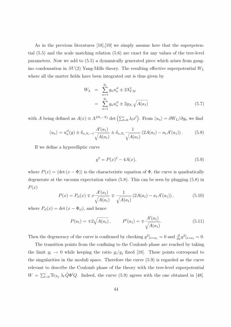
As in the previous literatures [18],[19] we simply assume here that the superpoten-

tial (5.5) and the scale matching relation (5.6) are exact for any values of the tree-level

parameters. Now we add to (5.5) a dynamically generated piece which arises from gaug-

ino condensation in SU(2) Yang-Mills theory. The resulting effective superpotential WL

where all the matter fields have been integrated out is thus given by

WL =Nc∑

n=1

gnucln ± 2Λ3

Y M

=Nc∑

n=1

gnucln ± 2gNc

√A(a1) (5.7)

with A being defined as A(x) ≡ Λ2Nc−Nf det(∑r

l=0 λlxl). From ⟨un⟩ = ∂WL/∂gn we find

⟨un⟩ = ucln (g) ± δn,Nc−1

A′(a1)√A(a1)

± δn,Nc

1√A(a1)

(2A(a1) − a1A′(a1)) . (5.8)

If we define a hyperelliptic curve

y2 = P (x)2 − 4A(x), (5.9)

where P (x) = ⟨det (x − Φ)⟩ is the characteristic equation of Φ, the curve is quadratically

degenerate at the vacuum expectation values (5.8). This can be seen by plugging (5.8) in

P (x)

P (x) = Pcl(x) ∓ xA′(a1)√A(a1)

∓ 1√A(a1)

(2A(a1) − a1A′(a1)) , (5.10)

where Pcl(x) = det (x − Φcl), and hence

P (a1) = ∓2√

A(a1) , P ′(a1) = ∓ A′(a1)√A(a1)

. (5.11)

Then the degeneracy of the curve is confirmed by checking y2|x=a1 = 0 and ∂∂x

y2|x=a1 = 0.

The transition points from the confining to the Coulomb phase are reached by taking

the limit gi → 0 while keeping the ratio gi/gj fixed [18]. These points correspond to

the singularities in the moduli space. Therefore the curve (5.9) is regarded as the curve

relevant to describe the Coulomb phase of the theory with the tree-level superpotential

W =∑r

l=0 TrNfλl QΦlQ. Indeed, the curve (5.9) agrees with the one obtained in [48].

44

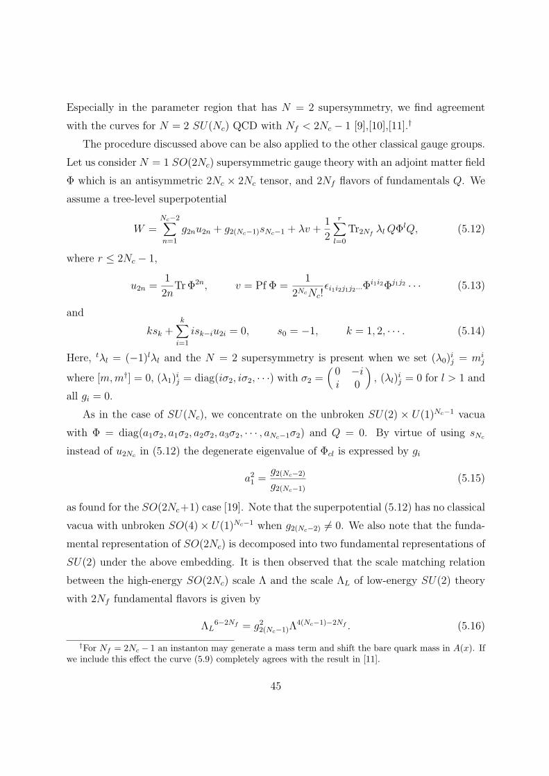
Especially in the parameter region that has N = 2 supersymmetry, we find agreement

with the curves for N = 2 SU(Nc) QCD with Nf < 2Nc − 1 [9],[10],[11].†

The procedure discussed above can be also applied to the other classical gauge groups.

Let us consider N = 1 SO(2Nc) supersymmetric gauge theory with an adjoint matter field

Φ which is an antisymmetric 2Nc × 2Nc tensor, and 2Nf flavors of fundamentals Q. We

assume a tree-level superpotential

W =Nc−2∑n=1

g2nu2n + g2(Nc−1)sNc−1 + λv +1

2

r∑l=0

Tr2Nfλl QΦlQ, (5.12)

where r ≤ 2Nc − 1,

u2n =1

2nTr Φ2n, v = Pf Φ =

1

2NcNc!ϵi1i2j1j2···Φ

i1i2Φj1j2 · · · (5.13)

and

ksk +k∑

i=1

isk−iu2i = 0, s0 = −1, k = 1, 2, · · · . (5.14)

Here, tλl = (−1)lλl and the N = 2 supersymmetry is present when we set (λ0)ij = mi

j

where [m,m†] = 0, (λ1)ij = diag(iσ2, iσ2, · · ·) with σ2 =

(0 −ii 0

), (λl)

ij = 0 for l > 1 and

all gi = 0.

As in the case of SU(Nc), we concentrate on the unbroken SU(2) × U(1)Nc−1 vacua

with Φ = diag(a1σ2, a1σ2, a2σ2, a3σ2, · · · , aNc−1σ2) and Q = 0. By virtue of using sNc

instead of u2Nc in (5.12) the degenerate eigenvalue of Φcl is expressed by gi

a21 =

g2(Nc−2)

g2(Nc−1)

(5.15)

as found for the SO(2Nc+1) case [19]. Note that the superpotential (5.12) has no classical

vacua with unbroken SO(4) × U(1)Nc−1 when g2(Nc−2) = 0. We also note that the funda-

mental representation of SO(2Nc) is decomposed into two fundamental representations of

SU(2) under the above embedding. It is then observed that the scale matching relation

between the high-energy SO(2Nc) scale Λ and the scale ΛL of low-energy SU(2) theory

with 2Nf fundamental flavors is given by

ΛL6−2Nf = g2

2(Nc−1)Λ4(Nc−1)−2Nf . (5.16)

†For Nf = 2Nc − 1 an instanton may generate a mass term and shift the bare quark mass in A(x). Ifwe include this effect the curve (5.9) completely agrees with the result in [11].

45

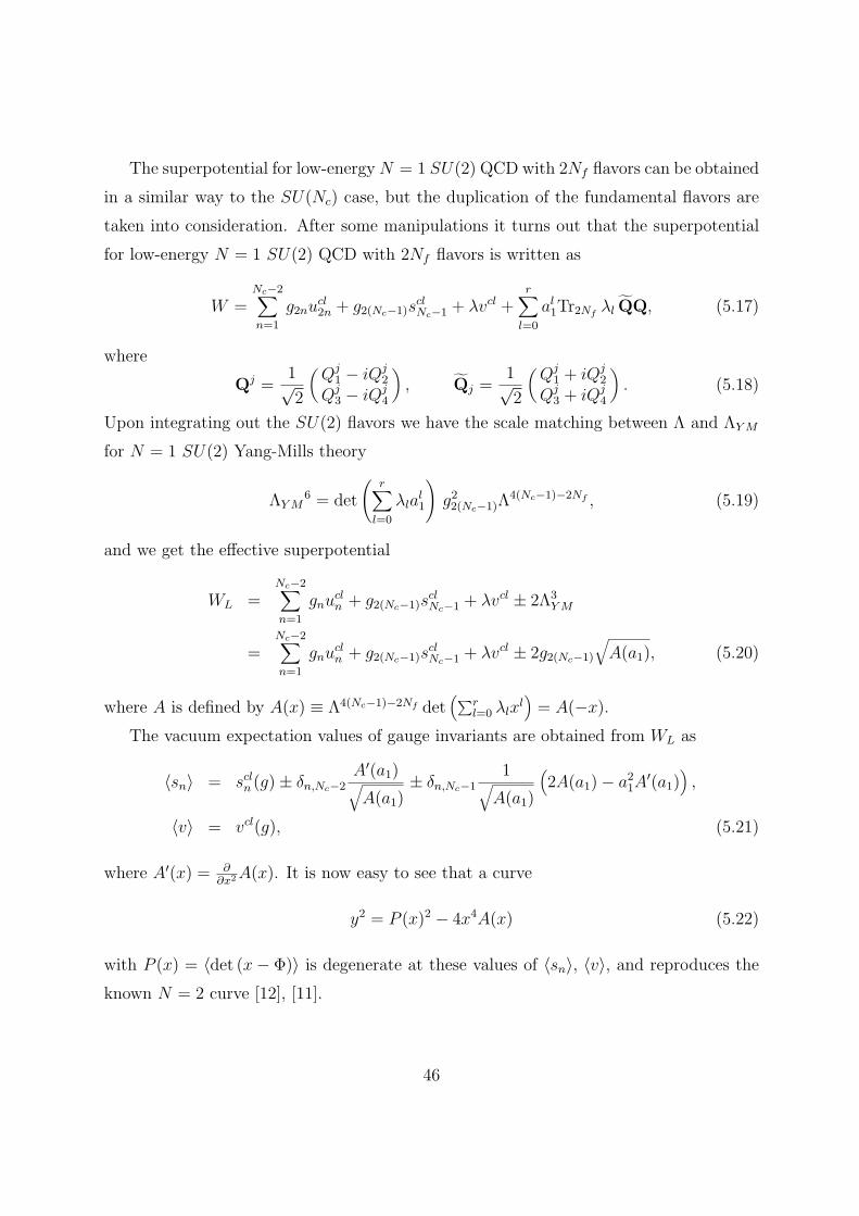
The superpotential for low-energy N = 1 SU(2) QCD with 2Nf flavors can be obtained

in a similar way to the SU(Nc) case, but the duplication of the fundamental flavors are

taken into consideration. After some manipulations it turns out that the superpotential

for low-energy N = 1 SU(2) QCD with 2Nf flavors is written as

W =Nc−2∑n=1

g2nucl2n + g2(Nc−1)s

clNc−1 + λvcl +

r∑l=0

al1Tr2Nf

λl QQ, (5.17)

where

Qj =1√2

(Qj

1 − iQj2

Qj3 − iQj

4

), Qj =

1√2

(Qj

1 + iQj2

Qj3 + iQj

4

). (5.18)

Upon integrating out the SU(2) flavors we have the scale matching between Λ and ΛY M

for N = 1 SU(2) Yang-Mills theory

ΛY M6 = det

(r∑

l=0

λlal1

)g22(Nc−1)Λ

4(Nc−1)−2Nf , (5.19)

and we get the effective superpotential

WL =Nc−2∑n=1

gnucln + g2(Nc−1)s

clNc−1 + λvcl ± 2Λ3

Y M

=Nc−2∑n=1

gnucln + g2(Nc−1)s

clNc−1 + λvcl ± 2g2(Nc−1)

√A(a1), (5.20)

where A is defined by A(x) ≡ Λ4(Nc−1)−2Nf det(∑r

l=0 λlxl)

= A(−x).

The vacuum expectation values of gauge invariants are obtained from WL as

⟨sn⟩ = scln (g) ± δn,Nc−2

A′(a1)√A(a1)

± δn,Nc−11√

A(a1)

(2A(a1) − a2

1A′(a1)

),

⟨v⟩ = vcl(g), (5.21)

where A′(x) = ∂∂x2 A(x). It is now easy to see that a curve

y2 = P (x)2 − 4x4A(x) (5.22)

with P (x) = ⟨det (x − Φ)⟩ is degenerate at these values of ⟨sn⟩, ⟨v⟩, and reproduces the

known N = 2 curve [12], [11].

46

The only difference between SO(2Nc) and SO(2Nc + 1) is that the gauge invariant

Pf Φ vanishes for SO(2Nc + 1). Thus, taking a tree-level superpotential

W =Nc−1∑n=1

g2nu2n + g2NcsNc +1

2

r∑l=0

Tr2Nfλl QΦlQ, r ≤ 2Nc, (5.23)

we focus on the unbroken SU(2) × U(1)Nc−1 vacuum which has the classical expectation

values Φ = diag(a1σ2, a1σ2, a2σ2, · · · , aNc−1σ2, 0) and Q = 0 [19]. As in the SO(2Nc)

case we make use of the scale matching relation between the high-energy scale Λ and the

low-energy N = 1 SU(2) Yang-Mills scale ΛY M

ΛY M6 = det

(r∑

l=0

λlal1

)g2Ncg2(Nc−1)Λ

2(2Nc−1−Nf ). (5.24)

As a result we find the effective superpotential

WL =Nc−1∑n=1

g2nucln + g2Ncs

clNc

± 2Λ3Y M

=Nc−1∑n=1

g2nucln + g2Ncs

clNc

± 2√

g2Ncg2(Nc−1)A(a1), (5.25)

where A is defined as A(x) ≡ Λ2(2Nc−1−Nf ) det(∑r

l=0 λlxl).

Noting the relation a21 = g2(Nc−1)/g2Nc [19] we calculate the vacuum expectation values

of gauge invariants

⟨sn⟩ = scln (g) ± δn,Nc−1

1√A(a1)

(A(a1)

a1

+ a1A′(a1)

)

± δn,Nc

1√A(a1)

(a1A(a1) − a3

1A′(a1)

). (5.26)

For these ⟨sn⟩ we observe the quadratic degeneracy of the curve

y2 =(

1

xP (x)

)2

− 4x2A(x), (5.27)

where P (x) = ⟨det (x − Φ)⟩. In the N = 2 limit we see agreement with the curve con-

structed in [12],[11]. The confining phase superpotential for the SO(5) gauge group was

obtained also in [26].

47

Let us now turn to Sp(2Nc) gauge theory. We take for matter content an adjoint field

Φ and 2Nf fundamental fields Q. The 2Nc × 2Nc tensor Φ is subject to tΦ = JΦJ with

J = diag(iσ2, · · · , iσ2). Our tree-level superpotential reads

W =Nc−1∑n=1

g2nu2n + g2NcsNc +1

2

r∑l=0

Tr2Nfλl QJΦlQ, (5.28)

where tλl = (−1)l+1λl and r ≤ 2Nc−1. The classical vacuum with the unbroken SU(2)×U(1)Nc−1 gauge group corresponds to

JΦ = diag(σ1a1, σ1a1, σ1a2, · · · , σ1aNc−1), σ1 =

(0 11 0

), (5.29)

where a21 = g2(Nc−1)/g2Nc . The scale ΛL for low-energy SU(2) theory with 2Nf flavors is

expressed as [19]

ΛL6−2Nf =

(g22Nc

g2(Nc−1)

)2

Λ2(2Nc+2−Nf ). (5.30)

There exists a subtle point in the analysis of Sp(2Nc) theory. When Sp(2Nc) is broken

to SU(2) × U(1)Nc−1 the instantons in the broken part of the gauge group play a role

since the index of the embedding of the unbroken SU(2) in Sp(2Nc) is larger than one (see

eq.(5.30)) [49],[50]. The possible instanton contribution to WL will be of the same order

in Λ as low-energy SU(2) gaugino condensation. Therefore even in the lowest quantum

corrections the instanton term must be added to WL.

For clarity we begin with discussing Sp(4) Yang-Mills theory. In this theory by the

symmetry and holomorphy the effective superpotential is determined to take the form

WL = f(

g4

g2Λ2

)g24

g2Λ6 with f being certain holomorphic function. If we assume that there

is only one-instanton effect, the precise form of WL including the low-energy gaugino

condensation effect may be given by

WL = 2g24

g2

Λ6 ± 2g24

g2

Λ6, (5.31)

as in the case of SO(4) ≃ SU(2) × SU(2) breaking to the diagonal SU(2). This is due

to the fact Sp(4) ≃ SO(5) and the natural embedding of SO(4) in SO(5). Our low-

energy SU(2) gauge group is identified with the one diagonally embedded in SO(4) ≃SU(2) × SU(2) [49],[51]. Accordingly, in Sp(2Nc) Yang-Mills theory, we first make the

48

matching at the scale of Sp(2Nc)/Sp(4) W bosons by taking all the a1 − ai large. Then

the low-energy superpotential is found to be

WL = Wcl + 2g2Nc

a21

Λ2(Nc+1) ± 2g2Nc

a21

Λ2(Nc+1). (5.32)

Let us turn on the coupling to fundamental flavors Q and evaluate the instanton

contribution. When flavor masses vanish there is a global O(2Nf ) ≃ SO(2Nf ) × Z2

symmetry. The couplings λl and instantons break a “parity” symmetry Z2. We treat this

Z2 as unbroken by assigning odd parity to the instanton factor Λ2Nc+2−Nf and O(2Nf )

charges to λl. Symmetry consideration then leads to the one-instanton factor proportional

to B(a1) where

B(x) = Λ2Nc+2−Nf Pf

( ∑l even

λlxl

). (5.33)

Note that B(x) is parity invariant since Pfaffian has odd parity. Thus the superpotential

for low-energy N = 1 SU(2) QCD with 2Nf flavors including the instanton effect turns

out to be

W =Nc−1∑n=1

g2nucl2n + g2Ncs

clNc

+r∑

l=0

al1Tr2Nf

λl QQ + 2g22Nc

g2(Nc−1)

B(a1), (5.34)

where

Qj =(

Qj1

Qj3

), Qj =

(Qj

2

Qj4

). (5.35)

When integrating out the SU(2) flavors, the scale matching relation between Λ and the

scale ΛY M of N = 1 SU(2) Yang-Mills theory becomes

ΛY M6 = det

(r∑

l=0

λlal1

) (g22Nc

g2(Nc−1)

)2

Λ2(2Nc+2−Nf ), (5.36)

and we finally obtain the effective superpotential

WL =Nc−1∑n=1

gnucln + g2Ncs

clNc

± 2Λ3Y M + 2

g22Nc

g2(Nc−1)

B(a1)

=Nc−1∑n=1

gnucln + g2Ncs

clNc

+ 2g22Nc

g2(Nc−1)

(B(a1) ±

√A(a1)

), (5.37)

where A(x) ≡ Λ2(2Nc+2−Nf ) det(∑r

l=0 λlxl).

49

The gauge invariant expectation values ⟨sn⟩ are

⟨sn⟩ = scln (g) + δn,Nc−1

1

a41

−2B(a1) + 2a21B

′(a1) ±1√

A(a1)

(−2A(a1) + a2

1A′(a1)

)+ δn,Nc

1

a21

4B(a1) − 2a21B

′(a1) ±1√

A(a1)

(4A(a1) − a2

1A′(a1)

) . (5.38)

Substituting these into a curve

x2y2 =(x2P (x) + 2B(x)

)2− 4A(x), (5.39)

we see that the curve is degenerate at (5.38). In this case too our result (5.39) agrees

with the N = 2 curve obtained in [11].

Before concluding this section, we should note that the effective superpotentials WL

obtained in this section are also confirmed in the approach based on the brane dynamics

[53, 54].

5.2 ADE gauge groups and various matters

Let us consider N = 1 gauge theory with the ADE gauge group and Nf flavors of chi-

ral matter multiplets Qi, Qj in addition to the adjoint matter Φ. We take a tree-level

superpotential

W =r∑

k=1

gkuk(Φ) +q∑

l=0

TrNfγl QΦl

RQ, (5.40)

where ΦR is a dR × dR matrix representation of Φ in R and (γl)ij, 1 ≤ i, j ≤ Nf , are the

coupling constants and q should be restricted so that QΦlRQ is irreducible in the sense

that it cannot be factored into gauge invariants. If we set (γ0)ij = mi

j with [m,m†] = 0,

(γ1)ij =

√2δi

j, (γl)ij = 0 for l > 1 and all gi = 0, (5.40) reduces to the superpotential in

N = 2 supersymmetric Yang-Mills theory with massive Nf hypermultiplets.

Let us focus on the classical vacua of the Coulomb phase with Q = Q = 0 and an

unbroken SU(2) × U(1)r−1 gauge group symmetry. The vacuum condition for Φ is given

by (4.82) and the classical vacuum takes the form as in the Yang-Mills case

ΦR = diag(a · λ1, a · λ2, · · · , a · λdR), (5.41)

50

where λi are the weights of the representation R. In this vacuum, we will evaluate

semiclassically the low-energy effective superpotential in the tree-level parameter region

where the Higgs mechanism occurs at very high energies and the adjoint matter field Φ is

quite heavy. Then the massive particles are integrated out and we get low-energy SU(2)

theory with flavors.

This integrating-out process results in the scale matching relation which is essentially

the same as the the Yang-Mills case (4.86) except that we here have to take into account

flavor loops. The one instanton factor in high-energy theory is given by Λ2h−l(R)Nf . Here

the index l(R) of the representation R is defined by l(R)δab = Tr(TaTb) where Ta is the

representation matrix of R with root vectors normalized as α2 = 2. The index is always

an integer [52]. The scale matching relation becomes

Λ3·2−l(R)Nf

L = g2rΛ

2h−l(R)Nf , (5.42)

where ΛL is the scale of low-energy SU(2) theory with massive flavors.

To consider the superpotential for low-energy SU(2) theory with Nf flavors we de-

compose the matter representation R of G in terms of the SU(2) subgroup. We have

R =nR⊕s=1

RsSU(2) ⊕ singlets, (5.43)

where RsSU(2) stands for a non-singlet SU(2) representation. Accordingly Qi is decom-

posed into SU(2) singlets and Qis (1 ≤ i ≤ Nf , 1 ≤ s ≤ nR) in an SU(2) representation

RsSU(2). Qi is decomposed in a similar manner. The singlet components are decoupled in

low-energy SU(2) theory.

The semiclassical superpotential for SU(2) theory with Nf flavors is now given by

W =r∑

k=1

gkuclk +

nR∑s=1

q∑l=0

(a · λRs)l TrNf

γl QsQs, (5.44)

where λRs is a weight of R which branches to the weights in RsSU(2). Here we assume that

R is a representation which does not break up into integer spin representations of SU(2);

otherwise we would be in trouble when γ0 = 0. The fundamental representations of ADE

groups except for E8 are in accord with this assumption.

We now integrate out massive flavors to obtain low-energy N = 1 SU(2) Yang-Mills

theory with the dynamical scale ΛY M . Reading off the flavor masses from (5.44) we get

51

the scale matching

Λ3·2Y M = g2

rA(a),

A(a) ≡ Λ2h−l(R)Nf

nR∏s=1

det

( q∑l=0

γl(a · λRs)l

)l(RsSU(2)

) , (5.45)

where l(RsSU(2)) is the index of Rs

SU(2) which is related to l(R) through

l(R) =nR∑s=1

l(RsSU(2)). (5.46)

The index of the spin m/2 representation of SU(2) is given by m(m + 1)(m + 2)/6.

Including the effect of SU(2) gaugino condensation we finally arrive at the effective

superpotential for low-energy SU(2) theory

WL = Wcl(g) ± 2Λ3Y M = Wcl(g) ± 2gr

√A(a), (5.47)

The expectation values ⟨uk⟩ = ∂WL/∂gk are found to be

⟨uj⟩ = uclj ± 2

∂√

A

∂g′j

, 1 ≤ j ≤ r − 1,

⟨ur⟩ = uclr ± 2

(√A + gr

r−1∑k=1

∂g′k

∂gr

∂√

A

∂g′k

)

= uclr ± 2

(√A −

r−1∑k=1

g′k

∂√

A

∂g′k

), (5.48)

where we have set g′k = gk/gr and used the fact that ucl

k and A are functions of g′k since

ai in (5.47) are solutions of (4.60) (see also (4.82)).

Let us show that the vacuum expectation values (5.48) obey the singularity condition

for the family of (r−1)-dimensional complex manifolds defined by W = 0 with coordinates

z, x1, · · · , xr−1 where

W = z +A(xn)

z−

r∑i=1

xi

(ui − ucl

i (xn)). (5.49)

Here we have introduced the variables xi (1 ≤ i ≤ r − 1) instead of g′i to express A(g′

n)

and ucli (g′

n), xr = 1 and ui are moduli parameters. The manifold W = 0 is singular when

∂W∂z

= 0,∂W∂xi

= 0. (5.50)

52

Then, if we set z = ±√

A(xk), xk = g′k and uj = ⟨uj⟩ it is easy to show that the singularity

conditions are satisfied

W| = ±2√

A(g′k) −

r∑i=1

g′i

(⟨ui⟩ − ucl

i (g′k)

)= 0,

∂W∂z

∣∣∣∣∣ = 0,

∂W∂xj

∣∣∣∣∣ = ± 1√A(g′

k)

∂A(g′k)

∂g′j

− ⟨uj⟩ +∂

∂g′j

(r∑

i=1

g′iu

cli (g′

k)

)

= −uclj (g′

k) + gr∂

∂gj

(Wcl(g)

gr

)= 0, 1 ≤ j ≤ r − 1. (5.51)

Thus the singularities of the manifold defined by W = 0 are parametrized by the expec-

tation values ⟨uk⟩.Let us explain how the known curves for SU(Nc) and SO(2Nc) supersymmetric QCD

are reproduced from (5.49). First we consider SU(Nc) theory with Nf fundamental flavors.

Here we denote the degree i Casimir by ui and correspondingly change the notations for

xj and g′j. It is shown in [20],[21] that

A = Λ2Nc−Nf detNf

( q∑l=0

(a1)lγl

), a1 = g′

Nc−1, (5.52)

and hence (5.49) becomes

W = z +A(xNc−1)

z−

Nc∑i=2

xi(ui − ucli (xn)). (5.53)

Since A depends only on xNc−1 one can eliminate other variables x1, · · · , xNc−2 by imposing

∂W/∂xj = 0 to get the relation

uclj (xn) = uj (5.54)

for 2 ≤ j ≤ Nc − 2, and then

W = z +A(xNc−1)

z− (uNc − ucl

Nc(xn)) − xNc−1(uNc−1 − ucl

Nc−1(xn)). (5.55)

Remember that

0 = det(a1 − Φcl

)= (a1)Nc − scl

2 (a1)Nc−1 − · · · − sclNc

, (5.56)

53

where

ksk +k∑

i=1

isk−1ui = 0, un =1

nTr Φn, k = 1, 2, · · · (5.57)

with s0 = −1 and s1 = u1 = 0. We see with the aid of (5.56) that

uclNc

+ xNc−1uclNc−1 = (ucl

Nc− scl

Nc) + xNc−1(u

clNc−1 − scl

Nc−1) + (sclNc

+ xNc−1sclNc−1)

= (uNc − sNc) + xNc−1(uNc−1 − sNc−1)

+((xNc−1)

Nc − s2(xNc−1)Nc−1 − · · · − sNc−2

), (5.58)

where (5.54) and the fact that sNc = uNc +(polynomial of uk, 2 ≤ k ≤ Nc − 2) have been

utilized. We now rewrite (5.55) as

W = z +A(x)

z− (uNc + xuNc−1) + (ucl

Nc+ xucl

Nc−1)

= z +A(x)

z+ xNc − s2x

Nc−1 − · · · − sNc , (5.59)

where xNc−1 was replaced by x for notational simplicity. This reproduces the hyperelliptic

curve derived in [48],[21] after making a change of variable y = z − A(x)/z and agrees

with the N = 2 curve obtained in [9],[10],[11] in the N = 2 limit .

Next we consider SO(2Nc) theory with 2Nf fundamental flavors Q. Following [21] we

take a tree-level superpotential

W =Nc−2∑n=k

g2ku2k + g2(Nc−1)sNc−1 + λv +1

2

q∑l=0

Tr2Nfγl QΦlQ, (5.60)

where

u2k =1

2kTr Φ2k, 1 ≤ k ≤ Nc − 1,

v = Pf Φ =1

2NcNc!ϵi1i2j1j2···Φ

i1i2Φj1j2 · · · (5.61)

and

ksk +k∑

i=1

isk−iu2i = 0, s0 = −1, k = 1, 2, · · · . (5.62)

According to [19] we have

(a1)2 = g′2(Nc−2), λ′ = 2

Nc−1∏j=2

(−iaj), vcl = −g′2(Nc−2)λ

′/2 (5.63)

54

and [21]

A = Λ4(Nc−1)−2Nf det2Nf

( q∑l=0

(a1)lγl

), (5.64)

and thus

W = z +A(xNc−2)

z−

Nc−1∑i=1

xi(u2i − ucl2i(xn)) − x(v − vcl(xn)), (5.65)

where λ′ = λ/g2(Nc−1) was replaced by x and g2i/g2(Nc−1) by xi.

In view of (5.64) we again notice that there are redundant variables which can be

eliminated by imposing the condition ∂W/∂xj = 0 so as to obtain

ucl2j(xn) = u2j (5.66)

for 1 ≤ j ≤ Nc − 3. We then find

W = z +A(xNc−2)

z− (u2(Nc−1) − ucl

2(Nc−1)(xn)) − xNc−2(u2(Nc−2) − ucl2(Nc−2)(xn))

− x(v − vcl(xn)). (5.67)

Using det(a1 − Φcl) = 0 we proceed further as in the SU(Nc) case. The final result reads

W = z +A(y)

z+

1

y

(yNc − s1y

Nc−1 − · · · − sNc−1y + vcl(xn)2)

−x(v − vcl(xn))

= z +A(y)

z− 1

4x2y + yNc−1 − s1y

Nc−2 − · · · − sNc−1 − vx, (5.68)

where we have set y = xNc−2 and used (5.63). It is now easy to check that imposing

∂W/∂x = 0 to eliminate x yields the known curve in [21] which has the correct N = 2

limit [12],[11].

It should be noted here that adding gaussian variables in (5.59) and (5.68) we have

WAn−1 = z +A(y1)

z+ yn

1 − s2yn−11 − · · · − sn + y2

2 + y23,

WDn = z +A(y1)

z− 1

4y2

2y1 + yn−11 − s1y

n−21 − · · · − sn−1 − vy2 + y2

3. (5.69)

These are equations describing ALE spaces of AD type fibered over CP1. Inclusion of

matter hypermultiplets makes fibrations more complicated than those for pure Yang-Mills

theory. For An the result is rather obvious, but for Dn it may be interesting to follow how

55

two variables y1, y2 come out naturally from (5.49). These variables are traced back to

coupling constants g2(n−2)/g2(n−1), λ/g2(n−1), respectively, and their degrees indeed agree

[y1] = [g2(n−2)/g2(n−1)] = 2, [y2] = [λ/g2(n−1)] = n − 2.

This observation suggests a possibility that even in the En case we may eliminate

redundant variables and derive the desired ALE form of Seiberg-Witten geometry directly

from (5.49). This issue is considered in the next subsection.

5.2.1 E6 theory with fundamental matters

In this subsection we will show that an extension of [28] enables us to obtain exceptional

Seiberg-Witten geometry with fundamental hypermultiplets. The resulting manifold takes

the form of a fibration of the ALE space of type E6.

Let us consider N = 1 E6 gauge theory with Nf fundamental matters Qi, Qj (1 ≤i, j ≤ Nf ) and an adjoint matter Φ. Qi, Qj are in 27 and 27, and Φ in 78 of E6. The

coefficient of the one-loop beta function is given by b = 24 − 6Nf , and hence the theory

is asymptotically free for Nf = 0, 1, 2, 3 and finite for Nf = 4. We take a tree-level

superpotential

W =∑k∈S

gksk(Φ) + TrNfγ0 QQ + TrNf

γ1 QΦQ, (5.70)

where S = 2, 5, 6, 8, 9, 12 denotes the set of degrees of E6 Casimirs sk(Φ) and gk, (γa)ji

(1 ≤ i, j ≤ Nf ) are coupling constants. A basis for the E6 Casimirs will be specified

momentarily. When we put (γ0)ij =

√2mi

j with [m,m†] = 0, (γ1)ji =

√2δj

i and all gk = 0,

(5.70) is reduced to the superpotential in N = 2 supersymmetric Yang-Mills theory with

massive Nf hypermultiplets.

We now look at the Coulomb phase with Q = Q = 0. Since Φ is restricted to take the

values in the Cartan subalgebra we express the classical value of Φ in terms of a vector ∗

a =6∑

i=1

aiαi (5.71)

with αi being the simple roots of E6. Then the classical vacuum is parametrized by

Φcl = diag (a · λ1, a · λ2, · · · , a · λ27), (5.72)

∗Our notation is slightly different from [28]. Here we use ai with lower index instead of ai in [28].

56

where λi are the weights for 27 of E6. For the notation of roots and weights we follow

[52]. We define a basis for the E6 Casimirs uk(Φ) by

u2 = − 1

12χ2, u5 = − 1

60χ5, u6 = −1

6χ6 +

1

6 · 122χ3

2,

u8 = − 1

40χ8 +

1

180χ2χ6 −

1

2 · 124χ4

2, u9 = − 1

7 · 62χ9 +

1

20 · 63χ2

2χ5,

u12 = − 1

60χ12 +

1

5 · 63χ2

6 +13

5 · 123χ2χ

25

+5

2 · 123χ2

2χ8 −1

3 · 64χ3

2χ6 +29

10 · 126χ6

2, (5.73)

where χn = Tr Φn. The standard basis wk(Φ) are written in terms of uk as follows

w2 =1

2u2, w5 = −1

4u5, w6 =

1

96

(u6 − u3

2

),

w8 =1

96

(u8 +

1

4u2u6 −

1

8u4

2

), w9 = − 1

48

(u9 −

1

4u2

2u5

),

w12 =1

3456

(u12 +

3

32u2

6 −3

4u2

2u8 −3

16u3

2u6 +1

16u6

2

). (5.74)

The basis uk and (5.74) were first introduced in [24].† In our superpotential (5.70) we

then set

s2 = w2, s5 = w5, s6 = w6, s8 = w8, s9 = w9, s12 = w12 −1

4w2

6. (5.75)

We will discuss later why this particular form is assumed.

The equations of motion are given by

∂W (a)

∂ai

=∑k∈S

gk∂sk(a)

∂ai

= 0. (5.76)

Let us focus on the classical vacua with an unbroken SU(2)×U(1)5 gauge symmetry. Fix

the SU(2) direction by choosing the simple root α1, then we have the vacuum condition

a · α1 = 2a1 − a2 = 0. (5.77)

It follows from (5.76), (5.77) that

g9

g12

=D1,9

D1,12

†The Casimirs u1, u2, u3, u4, u5, u6 in [24] are denoted here as u2, u5, u6, u8, u9, u12, respectively.

57

= −1

8

(2a1a5a4 − a4a

23 + a2

5a4 + a24a3 − a3a

26 + a2

3a6

−2a1a25 + 2a1a

26 − 2a2

4a1 − a5a24 − 2a1a3a6 + 2a4a3a1

),

g8

g12

=D1,8

D1,12

= − 1

48

(12a1a

25a4 − 6a2

1a25 − 6a2

1a26 − 4a3

1a3 + 4a33a1 + 2a3

3a4 + 2a33a6 − a4

4

−3a23a

26 − 3a2

3a24 − a4

3 − a46 − 12a1a5a

24 − 2a5a4a

26 + 8a1a3a

26 + 3a4

1

+6a21a4a3 − 8a4a

23a1 − 2a5a4a

23 − 2a2

4a3a6 + 6a21a5a4 − 2a4a3a

26

+2a5a24a3 − 2a2

5a3a6 + 2a4a23a6 − a4

5 − 2a25a4a3 − 2a2

1a23 − 6a2

1a24

+2a25a

26 + 2a2

4a26 + 2a2

5a23 + 6a2

1a3a6 − 8a1a23a6 + 8a2

4a3a1 − 4a25a1a3

+2a5a4a3a6 + 4a5a4a1a3 + 2a3a34 − 3a2

4a25 + 2a4a

35 + 2a3

4a5 + 2a36a3

),

g6

g12

=D1,6

D1,12

=1

192

(4a3

3a1a25 − 18a3

4a21a5 + 13a4

3a21 − a4

3a25 − 7a3

3a36 + 9a2

1a46 + · · ·

), (5.78)

where D1,k is the cofactor for a (1, k) element of the 6× 6 matrix [∂si(a)/∂aj], i ∈ S and

j = 1, . . . , 6 [28]. In (5.78) the explicit expression for g6/g12 is too long to be presented

here, and hence suppressed. Denoting y1 = g9/g12, y2 = g8/g12, y3 = g6/g12, we find that

the others are expressed in terms of y1, y2

g2

g12

=D2,2

D2,12

= y21y2,

g5

g12

=D2,5

D2,12

= y1y2. (5.79)

This means that our superpotential specified with Casimirs (5.75) realizes the SU(2) ×U(1)5 vacua only when the coupling constants are subject to the relation (5.79).

Notice that reading off degrees of y1, y2, y3 from (5.78) gives [y1] = 3, [y2] = 4, [y3] = 6.

Thus, if we regard y1, y2, y3 as variables to describe the E6 singularity, (5.78) and (5.79)

may be identified as relevant monomials in versal deformations of the E6 singularity. In

fact we now point out an intimate relationship between classical solutions corresponding

to the symmetry breaking E6 ⊃ SU(2) × U(1)5 and the E6 singularity. For this we

examine the superpotential (5.40) at classical solutions

Wcl = g12

∑k∈S

(gk

g12

)scl

k (a)

= g12

(scl2 y2

1y2 + scl5 y1y2 + scl

6 y3 + scl8 y2 + scl

9 y1 + scl12

). (5.80)

58

Evaluating the RHS with the use of (5.77)-(5.79) leads to

Wcl = −g12

(2y2

1y3 + y32 − y2

3

). (5.81)

It is also checked explicitly that

−4y1y3 = 2scl2 y1y2 + scl

5 y2 + scl9 ,

−3y22 = scl

2 y21 + scl

5 y1 + scl8 ,

−2y21 + 2y3 = scl

6 . (5.82)

To illustrate the meaning of (5.80)-(5.82) let us recall the standard form of versal

deformations of the E6 singularity

WE6(x1, x2, x3; w) = x41 +x3

2 +x23 +w2 x2

1x2 +w5 x1x2 +w6 x21 +w8 x2 +w9 x1 +w12, (5.83)

where the deformation parameters wk are related to the E6 Casimirs via (5.74) [24]. Then

what we have observed in (5.80)-(5.82) is that when we express wk in terms of ai as

wk = wclk (a) the equations

WE6 =∂WE6

∂x1

=∂WE6

∂x2

=∂WE6

∂x3

= 0 (5.84)

can be solved by ‡

x1 = y1(a), x2 = y2(a), x3 = i

(y3(a) − y1(a)2 − scl

6 (a)

2

)(5.85)

under the condition (5.77). This observation plays a crucial role in our analysis.

When applying the technique of confining phase superpotentials we usually take all

coupling constants gk as independent moduli parameters. To deal with N = 1 E6 theory

with fundamental matters, however, we find it appropriate to proceed as follows. First

of all, motivated by the above observations for classical solutions, we keep three coupling

constants g′6 = g6/g12, g′

8 = g8/g12 and g′9 = g9/g12 adjustable while the rest is fixed as

g′2 = g′

8g′29 , g′

5 = g′8g

′9 with g′

k = gk/g12. Taking this parametrization it is seen that the

equations of motion are satisfied by virtue of (5.79) in the SU(2) × U(1)5 vacua (5.77).

‡We have observed a similar relation between the symmetry breaking solutions SU(r+1) (or SO(2r))⊃ SU(2) × U(1)r−1 and the Ar (or Dr) singularity.

59

Note here that originally there exist six classical moduli ai among which one is fixed by

(5.77) and three are converted to g′9 = y1(a), g′

8 = y2(a) and g′6 = y3(a), and hence we are

left with two classical moduli which will be denoted as ξi. Without loss of generality one

may choose ξ2 = scl2 (a) and ξ5 = scl

5 (a).

We now evaluate the low-energy effective superpotential in the SU(2) × U(1)5 vacua.

U(1) photons decouple in the integrating-out process. The standard procedure yields the

effective superpotential for low-energy SU(2) theory [18],[28]

WL = −g12

(2y2

1y3 + y32 − y2

3

)± 2Λ3

Y M , (5.86)

where the second term takes account of SU(2) gaugino condensation with ΛY M being the

dynamical scale for low-energy SU(2) Yang-Mills theory. The low-energy scale ΛY M is

related to the high-energy scale Λ through the scale matching [28]

Λ6Y M = g2

12A(a),

A(a) ≡ Λ24−6Nf

6∏s=1

detNf(γ0 + γ1(a · λs)) , (5.87)

where λs are weights of 27 which branch to six SU(2) doublets respectively under E6 ⊃SU(2) × U(1)5. Explicitly they are given in the Dynkin basis as

λ1 = (1, 0, 0, 0, 0, 0), λ2 = (1, −1, 0, 0, 1, 0),

λ3 = (1, −1, 0, 1, −1, 0), λ4 = (1, −1, 1, −1, 0, 0),

λ5 = (1, 0, −1, 0, 0, 1), λ6 = (1, 0, 0, 0, 0, −1). (5.88)

Notice that∑6

s=1 λs = 3α1.

Let us first discuss the Nf = 0 case, i.e. E6 pure Yang-Mills theory, for which A(a) in

(5.87) simply equals Λ24. The vacuum expectation values are calculated from (5.86)

∂WL

∂g12

= ⟨W (y1, y2, y3; s)⟩ = −(2y2

1y3 + y32 − y2

3

)± 2Λ12,

1

g12

∂WL

∂y1

= ⟨∂W (y1, y2, y3; s)

∂y1

⟩ = −4y1y3,

1

g12

∂WL

∂y2

= ⟨∂W (y1, y2, y3; s)

∂y2

⟩ = −3y22,

1

g12

∂WL

∂y3

= ⟨∂W (y1, y2, y3; s)

∂y3

⟩ = −2y21 + 2y3, (5.89)

60

where y1, y2, y3 and g12 have been treated as independent parameters as discussed before

and

W (y1, y2, y3; s) = s2 y21y2 + s5 y1y2 + s6 y3 + s8 y2 + s9 y1 + s12. (5.90)

Define a manifold by W0 = 0 with four coordinate variables z, y1, y2, y3 ∈ C and

W0 ≡ z +Λ24

z−

(2y2

1y3 + y32 − y2

3 + W (y1, y2, y3; s))

= 0. (5.91)

It is easy to show that the expectation values (5.89) parametrize the singularities of the

manifold where∂W0

∂z=

∂W0

∂y1

=∂W0

∂y2

=∂W0

∂y3

= 0. (5.92)

Making a change of variables y1 = x1, y2 = x2, y3 = −ix3 + x21 + s6/2 in (5.91) we have

z +Λ24

z− WE6(x1, x2, x3; w) = 0. (5.93)

Thus the ALE space description of N = 2 E6 Yang-Mills theory [29],[24] is obtained from

the N = 1 confining phase superpotential.

We next turn to considering the fundamental matters. In the N = 2 limit we have

A(a) = Λ24−6Nf · 8Nf∏Nf

i=1 f(a,mi) with f(a, m) =∏6

s=1(m + a · λs). After some algebra

we find

f(a,m) = m6 + 2ξ2m4 − 8m3y1 +

(ξ22 − 12y2

)m2 + 4ξ5m − 4y2ξ2 − 8y3, (5.94)

where we have used (5.75)-(5.78). Let us recall that, in viewing (5.86), we think of

(y1, y2, y3, ξ2, ξ5, g12) as six independent parameters. Then the quantum expectation values

are given by

∂WL

∂g12

= ⟨W (y1, y2, y3; s)⟩ = −(2y2

1y3 + y32 − y2

3

)± 2

√A(y1, y2, y3; ξ,m),

1

g12

∂WL

∂y1

= ⟨∂W (y1, y2, y3; s)

∂y1

⟩ = −4y1y3 ± 2∂

∂y1

√A(y1, y2, y3; ξ,m),

1

g12

∂WL

∂y2

= ⟨∂W (y1, y2, y3; s)

∂y2

⟩ = −3y22 ± 2

∂

∂y2

√A(y1, y2, y3; ξ,m),

1

g12

∂WL

∂y3

= ⟨∂W (y1, y2, y3; s)

∂y3

⟩ = −2y21 + 2y3 ± 2

∂

∂y3

√A(y1, y2, y3; ξ,m). (5.95)

61

Similarly to the Nf = 0 case one can check that these expectation values satisfy the

singularity condition for a manifold defined by

z +1

zA(y1, y2, y3; ξ,m) −

(2y2

1y3 + y32 − y2

3 + W (y1, y2, y3; s))

= 0. (5.96)

Note that sk in W are quantum moduli parameters. What about ξ2, ξ5 in the one-

instanton factor A? Classically we have ξi = scli as was seen before. The issue is thus

whether the classical relations ξi = scli receive any quantum corrections at the singularities.

If there appear no quantum corrections, ξi in A can be replaced by quantum moduli

parameters si. Let us simply assume here that ξi = scli = ⟨si⟩ for i = 2, 5 in the N = 1

SU(2)×U(1)5 vacua. This assumption seems quite plausible as long as we have inspected

possible forms of quantum corrections due to gaugino condensates.

Now we find that Seiberg-Witten geometry of N = 2 supersymmetric QCD with gauge

group E6 is described by

z +1

zA(x1, x2, x3; w,m) − WE6(x1, x2, x3; w) = 0, (5.97)

where a change of variables from yi to xi as in (5.93) has been made in (5.96) and

A(x1, x2, x3; w,m)

= Λ24−6Nf · 8Nf

Nf∏i=1

(mi

6 + 2w2mi4 − 8mi

3x1 +(w2

2 − 12x2

)mi

2

+4w5mi − 4w2x2 − 8(x21 − ix3 + w6/2)

). (5.98)

The manifold takes the form of ALE space of type E6 fibered over the base CP1. Note

an intricate dependence of the fibering data over CP1 on the hypermultiplet masses.

This is in contrast with the ALE space description of N = 2 SU(Nc) and SO(2Nc)

gauge theories with fundamental matters. In (5.97), letting mi → ∞ while keeping

Λ24−6Nf∏Nf

i=1 m6i ≡ Λ24

0 finite we recover the pure Yang-Mills result (5.93).

As a non-trivial check of our proposal (5.97) let us examine the semi-classical singu-

larities. In the semi-classical limit Λ → 0 the discriminant ∆ for (5.97) is expected to

take the form ∆ ∝ ∆G∆M where ∆G is a piece arising from the classical singularities

associated with the gauge symmetry enhancement and ∆M represents the semi-classical

62

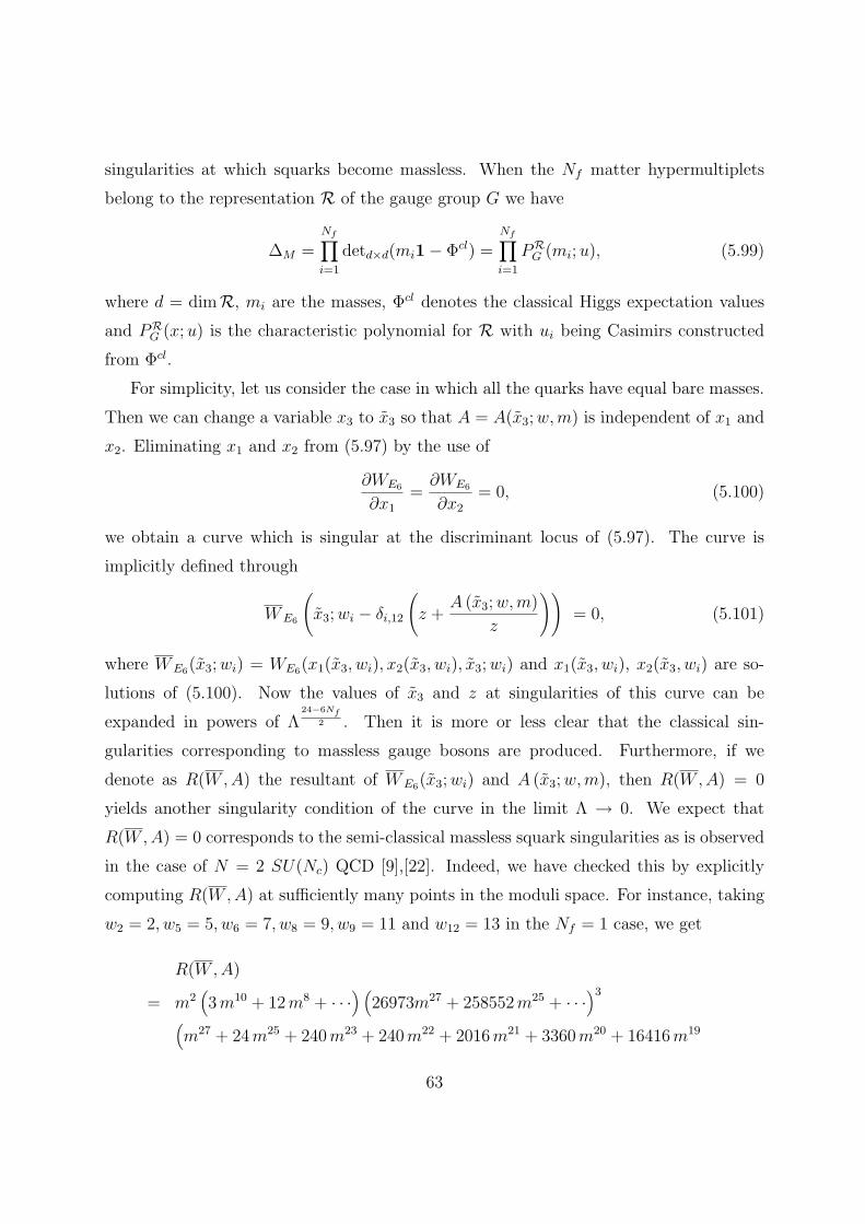
singularities at which squarks become massless. When the Nf matter hypermultiplets

belong to the representation R of the gauge group G we have

∆M =Nf∏i=1

detd×d(mi1 − Φcl) =Nf∏i=1

PRG (mi; u), (5.99)

where d = dimR, mi are the masses, Φcl denotes the classical Higgs expectation values

and PRG (x; u) is the characteristic polynomial for R with ui being Casimirs constructed

from Φcl.

For simplicity, let us consider the case in which all the quarks have equal bare masses.

Then we can change a variable x3 to x3 so that A = A(x3; w,m) is independent of x1 and

x2. Eliminating x1 and x2 from (5.97) by the use of

∂WE6

∂x1

=∂WE6

∂x2

= 0, (5.100)

we obtain a curve which is singular at the discriminant locus of (5.97). The curve is

implicitly defined through

WE6

(x3; wi − δi,12

(z +

A (x3; w,m)

z

))= 0, (5.101)

where WE6(x3; wi) = WE6(x1(x3, wi), x2(x3, wi), x3; wi) and x1(x3, wi), x2(x3, wi) are so-

lutions of (5.100). Now the values of x3 and z at singularities of this curve can be

expanded in powers of Λ24−6Nf

2 . Then it is more or less clear that the classical sin-

gularities corresponding to massless gauge bosons are produced. Furthermore, if we

denote as R(W,A) the resultant of WE6(x3; wi) and A (x3; w,m), then R(W,A) = 0

yields another singularity condition of the curve in the limit Λ → 0. We expect that

R(W,A) = 0 corresponds to the semi-classical massless squark singularities as is observed

in the case of N = 2 SU(Nc) QCD [9],[22]. Indeed, we have checked this by explicitly

computing R(W,A) at sufficiently many points in the moduli space. For instance, taking

w2 = 2, w5 = 5, w6 = 7, w8 = 9, w9 = 11 and w12 = 13 in the Nf = 1 case, we get

R(W,A)

= m2(3 m10 + 12 m8 + · · ·

) (26973m27 + 258552m25 + · · ·

)3

(m27 + 24 m25 + 240 m23 + 240 m22 + 2016 m21 + 3360m20 + 16416m19

63

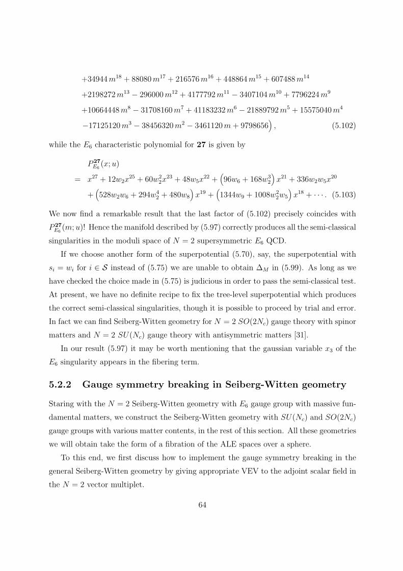
+34944 m18 + 88080m17 + 216576m16 + 448864m15 + 607488m14

+2198272m13 − 296000m12 + 4177792m11 − 3407104m10 + 7796224m9

+10664448m8 − 31708160m7 + 41183232m6 − 21889792m5 + 15575040m4

−17125120m3 − 38456320m2 − 3461120m + 9798656), (5.102)

while the E6 characteristic polynomial for 27 is given by

P 27E6

(x; u)

= x27 + 12w2x25 + 60w2

2x23 + 48w5x

22 +(96w6 + 168w3

2

)x21 + 336w2w5x

20

+(528w2w6 + 294w4

2 + 480w8

)x19 +

(1344w9 + 1008w2

2w5

)x18 + · · · . (5.103)

We now find a remarkable result that the last factor of (5.102) precisely coincides with

P 27E6

(m; u)! Hence the manifold described by (5.97) correctly produces all the semi-classical

singularities in the moduli space of N = 2 supersymmetric E6 QCD.

If we choose another form of the superpotential (5.70), say, the superpotential with

si = wi for i ∈ S instead of (5.75) we are unable to obtain ∆M in (5.99). As long as we

have checked the choice made in (5.75) is judicious in order to pass the semi-classical test.

At present, we have no definite recipe to fix the tree-level superpotential which produces

the correct semi-classical singularities, though it is possible to proceed by trial and error.

In fact we can find Seiberg-Witten geometry for N = 2 SO(2Nc) gauge theory with spinor

matters and N = 2 SU(Nc) gauge theory with antisymmetric matters [31].

In our result (5.97) it may be worth mentioning that the gaussian variable x3 of the

E6 singularity appears in the fibering term.

5.2.2 Gauge symmetry breaking in Seiberg-Witten geometry

Staring with the N = 2 Seiberg-Witten geometry with E6 gauge group with massive fun-

damental matters, we construct the Seiberg-Witten geometry with SU(Nc) and SO(2Nc)

gauge groups with various matter contents, in the rest of this section. All these geometries

we will obtain take the form of a fibration of the ALE spaces over a sphere.

To this end, we first discuss how to implement the gauge symmetry breaking in the

general Seiberg-Witten geometry by giving appropriate VEV to the adjoint scalar field in

the N = 2 vector multiplet.

64

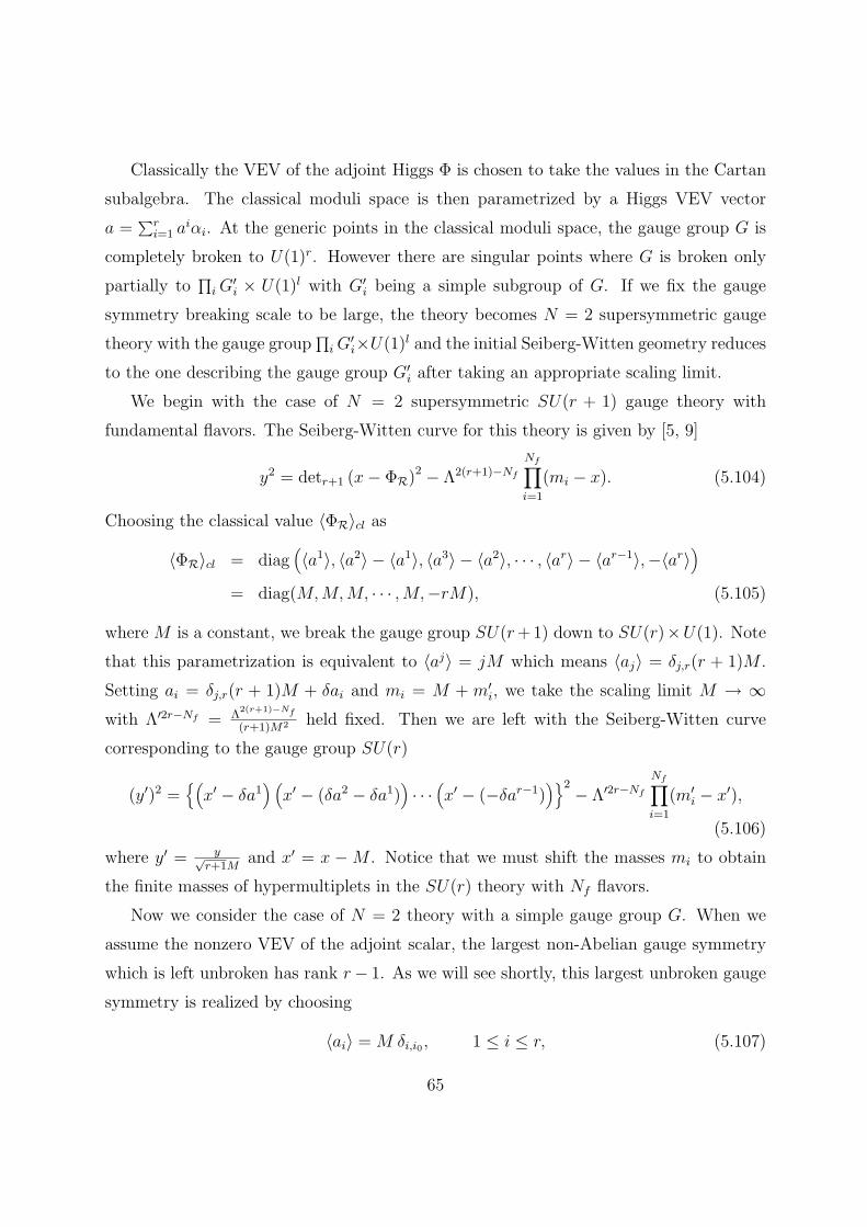
Classically the VEV of the adjoint Higgs Φ is chosen to take the values in the Cartan

subalgebra. The classical moduli space is then parametrized by a Higgs VEV vector

a =∑r

i=1 aiαi. At the generic points in the classical moduli space, the gauge group G is

completely broken to U(1)r. However there are singular points where G is broken only

partially to∏

i G′i × U(1)l with G′

i being a simple subgroup of G. If we fix the gauge

symmetry breaking scale to be large, the theory becomes N = 2 supersymmetric gauge

theory with the gauge group∏

i G′i×U(1)l and the initial Seiberg-Witten geometry reduces

to the one describing the gauge group G′i after taking an appropriate scaling limit.

We begin with the case of N = 2 supersymmetric SU(r + 1) gauge theory with

fundamental flavors. The Seiberg-Witten curve for this theory is given by [5, 9]

y2 = detr+1 (x − ΦR)2 − Λ2(r+1)−Nf

Nf∏i=1

(mi − x). (5.104)

Choosing the classical value ⟨ΦR⟩cl as

⟨ΦR⟩cl = diag(⟨a1⟩, ⟨a2⟩ − ⟨a1⟩, ⟨a3⟩ − ⟨a2⟩, · · · , ⟨ar⟩ − ⟨ar−1⟩,−⟨ar⟩

)= diag(M,M,M, · · · ,M,−rM), (5.105)

where M is a constant, we break the gauge group SU(r +1) down to SU(r)×U(1). Note

that this parametrization is equivalent to ⟨aj⟩ = jM which means ⟨aj⟩ = δj,r(r + 1)M .

Setting ai = δj,r(r + 1)M + δai and mi = M + m′i, we take the scaling limit M → ∞

with Λ′2r−Nf = Λ2(r+1)−Nf

(r+1)M2 held fixed. Then we are left with the Seiberg-Witten curve

corresponding to the gauge group SU(r)

(y′)2 =(

x′ − δa1) (

x′ − (δa2 − δa1))· · ·

(x′ − (−δar−1)

)2− Λ′2r−Nf

Nf∏i=1

(m′i − x′),

(5.106)

where y′ = y√r+1M

and x′ = x − M . Notice that we must shift the masses mi to obtain

the finite masses of hypermultiplets in the SU(r) theory with Nf flavors.

Now we consider the case of N = 2 theory with a simple gauge group G. When we

assume the nonzero VEV of the adjoint scalar, the largest non-Abelian gauge symmetry

which is left unbroken has rank r − 1. As we will see shortly, this largest unbroken gauge

symmetry is realized by choosing

⟨ai⟩ = M δi,i0 , 1 ≤ i ≤ r, (5.107)

65

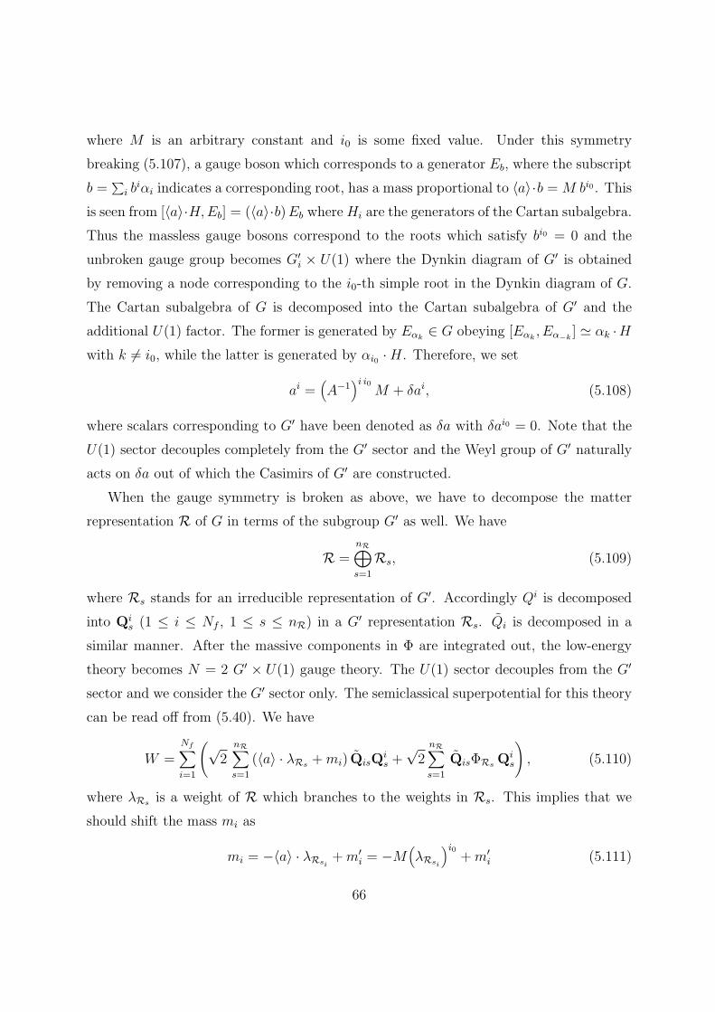
where M is an arbitrary constant and i0 is some fixed value. Under this symmetry

breaking (5.107), a gauge boson which corresponds to a generator Eb, where the subscript

b =∑

i biαi indicates a corresponding root, has a mass proportional to ⟨a⟩·b = M bi0 . This

is seen from [⟨a⟩·H,Eb] = (⟨a⟩·b) Eb where Hi are the generators of the Cartan subalgebra.

Thus the massless gauge bosons correspond to the roots which satisfy bi0 = 0 and the

unbroken gauge group becomes G′i × U(1) where the Dynkin diagram of G′ is obtained

by removing a node corresponding to the i0-th simple root in the Dynkin diagram of G.

The Cartan subalgebra of G is decomposed into the Cartan subalgebra of G′ and the

additional U(1) factor. The former is generated by Eαk∈ G obeying [Eαk

, Eα−k] ≃ αk ·H

with k = i0, while the latter is generated by αi0 · H. Therefore, we set

ai =(A−1

)i i0M + δai, (5.108)

where scalars corresponding to G′ have been denoted as δa with δai0 = 0. Note that the

U(1) sector decouples completely from the G′ sector and the Weyl group of G′ naturally

acts on δa out of which the Casimirs of G′ are constructed.

When the gauge symmetry is broken as above, we have to decompose the matter

representation R of G in terms of the subgroup G′ as well. We have

R =nR⊕s=1

Rs, (5.109)

where Rs stands for an irreducible representation of G′. Accordingly Qi is decomposed

into Qis (1 ≤ i ≤ Nf , 1 ≤ s ≤ nR) in a G′ representation Rs. Qi is decomposed in a

similar manner. After the massive components in Φ are integrated out, the low-energy

theory becomes N = 2 G′ × U(1) gauge theory. The U(1) sector decouples from the G′

sector and we consider the G′ sector only. The semiclassical superpotential for this theory

can be read off from (5.40). We have

W =Nf∑i=1

(√2

nR∑s=1

(⟨a⟩ · λRs + mi) QisQis +

√2

nR∑s=1

QisΦRs Qis

), (5.110)

where λRs is a weight of R which branches to the weights in Rs. This implies that we

should shift the mass mi as

mi = −⟨a⟩ · λRsi+ m′

i = −M(λRsi

)i0+ m′

i (5.111)

66

to obtain the G′ theory with appropriate matter hypermultiplets. Note that we can

choose Rsifor each hypermultiplet separately. This enables us to obtain the Nf matters

in different representations of G′ from the Nf matters in a single representation of G.

In the limit M → ∞, some hypermultiplets have infinite masses and decouple from the

theory. Then the superpotential (5.110) becomes

W =√

2Nf∑i=1

m′i Qi si

Qisi

+√

2Nf∑i=1

Qi siΦRsi

Qisi, (5.112)

and the resulting theory becomes N = 2 theory with gauge group G′ with hypermultiplets

belonging to the representation Rsi. Note that ⟨a⟩ · λRs is proportional to its additional

U(1) charge.

In the known cases, the low-energy effective theory in the Coulomb phase is described

by the Seiberg-Witten geometry which is described by a three-dimensional complex man-

ifold in the form of the ALE space of ADE type fibered over CP1

z +1

zΛ2h−l(R)Nf

Nf∏i=1

XRG (x1, x2, x3; a,mi) − WG(x1, x2, x3; a) = 0, (5.113)

where z parametrizes CP1, h is the dual Coxeter number of G and l(R) is the index of the

representation R of the matter. Here WG(x1, x2, x3; a) = 0 is a simple singularity of type

G and XRG (x1, x2, x3; a,mi) is some polynomial of the indicated variables. Note that the

simple singularity WG depends only on the gauge group G, but the XRG (x1, x2, x3; a,mi)

depends on the matter content of the theory.

Starting with (5.113) let us consider the symmetry breaking in the Seiberg-Witten

geometry. In the limit M → ∞, the gauge symmetry G is reduced to the smaller one G′.

The Seiberg-Witten geometry is also reduced to the one with gauge symmetry G′ in this

limit. We can see this by substituting a = ⟨a⟩ + δa into (5.113) and keeping the leading

order in M . To leave the j-th flavor of hypermultiplets in the G′ theory, its mass mj is

also shifted as in (5.111). After taking the appropriate coordinate (x′1, x

′2, x

′3) we should

have

WG(x1, x2, x3; a) = Mh−h′WG′(x′

1, x′2, x

′3; δa) + o(Mh−h′

),

XRG (x1, x2, x3; a,mj) = M l(R)−l(Rsj )X

Rsj

G′ (x′1, x

′2, x

′3; δa,m′

j) + o(M l(R)−l(Rsj )),

(5.114)

67

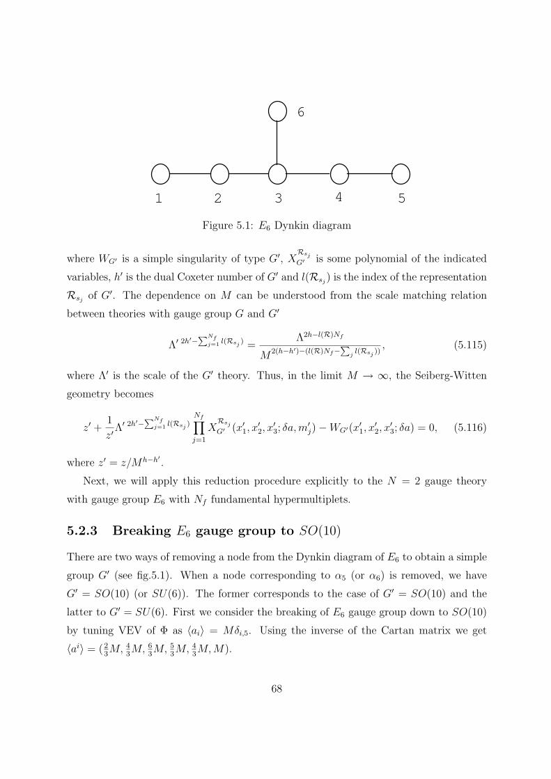
1 2 3 4 5

6

Figure 5.1: E6 Dynkin diagram

where WG′ is a simple singularity of type G′, XRsj

G′ is some polynomial of the indicated

variables, h′ is the dual Coxeter number of G′ and l(Rsj) is the index of the representation

Rsjof G′. The dependence on M can be understood from the scale matching relation

between theories with gauge group G and G′

Λ′ 2h′−∑Nf

j=1 l(Rsj ) =Λ2h−l(R)Nf

M2(h−h′)−(l(R)Nf−∑

jl(Rsj ))

, (5.115)

where Λ′ is the scale of the G′ theory. Thus, in the limit M → ∞, the Seiberg-Witten

geometry becomes

z′ +1

z′Λ′ 2h′−

∑Nfj=1 l(Rsj )

Nf∏j=1

XRsj

G′ (x′1, x

′2, x

′3; δa,m′

j) − WG′(x′1, x

′2, x

′3; δa) = 0, (5.116)

where z′ = z/Mh−h′.

Next, we will apply this reduction procedure explicitly to the N = 2 gauge theory

with gauge group E6 with Nf fundamental hypermultiplets.

5.2.3 Breaking E6 gauge group to SO(10)

There are two ways of removing a node from the Dynkin diagram of E6 to obtain a simple

group G′ (see fig.5.1). When a node corresponding to α5 (or α6) is removed, we have

G′ = SO(10) (or SU(6)). The former corresponds to the case of G′ = SO(10) and the

latter to G′ = SU(6). First we consider the breaking of E6 gauge group down to SO(10)

by tuning VEV of Φ as ⟨ai⟩ = Mδi,5. Using the inverse of the Cartan matrix we get

⟨ai⟩ = (23M, 4

3M, 6

3M, 5

3M, 4

3M,M).

68

The Seiberg-Witten geometry for N = 2 gauge theory with gauge group E6 with Nf

fundamental matters is proposed in [31]

z +1

zΛ24−6Nf

Nf∏i=1

X27E6

(x1, x2, x3; w,mi) − WE6(x1, x2, x3; w) = 0, (5.117)

where

WE6(x1, x2, x3; w) = x41+x3

2+x23+w2 x2

1x2+w5 x1x2+w6 x21+w8 x2+w9 x1+w12, (5.118)

and

X27E6

(x1, x2, x3; w,mi)

= 8(mi

6 + 2w2mi4 − 8mi

3x1 +(w2

2 − 12x2

)mi

2

+4w5mi − 4w2x2 − 8(x21 − ix3 + w6/2)

). (5.119)

Here wk = wk(a) is the degree k Casimir of E6 made out of aj and the degrees of x1, x2

and x3 are 3, 4 and 6 respectively. Now, substituting ai = Mδi,5 + δai into wk(a) and

setting δa5 = 0, we expand WE6 and X27E6

in M . As discussed in the previous section,

there should be coordinates (x′1, x

′2, x

′3) which can eliminate the terms depending upon

M l (5 ≤ l ≤ 12) in WE6 . Indeed, we can find such coordinates as,

x1 = − 2

27M3 − 1

4Mx′

1 −1

6Mw2,

x2 =1

54M4 +

1

12M2x′

1 +1

9M2w2 +

1

8x′

2 +1

6w2

2,

x3 = −i1

16M2x′

3. (5.120)

Then the E6 singularity WE6 is written as

WE6(x1, x2, x3; w) =(

1

4M

)4

WD5(x′1, x

′2, x

′3; v) + O(M3), (5.121)

where

WD5(x1, x2, x3; v) = x14 + x1x2

2 − x32 + v2x1

3 + v4x21 + v6x1 + v8 + v5x2, (5.122)

and vk = vk(δa) is the degree k Casimir of SO(10) constructed from δai. If we represent

Φ as a 10×10 matrix of the fundamental representation of SO(10), we have v2l = 12l

TrΦ2l

69

and v5 = 2iPfΦ. Thus we see in the M → ∞ limit that the Seiberg-Witten geometry

for N = 2 pure Yang-Mills theory with gauge group E6 becomes that with gauge group

SO(10).

Next we consider the effect of symmetry breaking in the matter sector. The funda-

mental representation 27 of E6 is decomposed into the representations of SO(10)× U(1)

as

27 = 16− 13⊕ 10 2

3⊕ 1− 4

3, (5.123)

where the subscript denotes the U(1) charge α5 ·λi (1 ≤ i ≤ 27). The indices of the spinor

representation 16 and the vector representation 10 are four and two, respectively. Let us

first take the scaling limit in such a way that the spinor matters of SO(10) survive. Then

the terms with M l (l ≥ 3) in X27E6

must be absent after a change of variables (5.120) and

the mass shift mi = 13M + msi (see (5.111)). In fact we find that

X27E6

(x1, x2, x3; w,mi) = M2X16D5

(x′1, x

′2, x

′3; v,msi) + O(M), (5.124)

where

X16D5

(x1, x2, x3; v,m) = m4 +(x1 +

1

2v2

)m2 −mx2 +

1

2x3 −

1

4

(v4 −

1

4v2

2

)− 1

4v2x1 −

1

2x2

1.

(5.125)

In order to make the vector matter of SO(10) survive, we shift masses as mi = −23M+mvi.

The result reads

X27E6

(x1, x2, x3; v,mi) = M4X10D5

(x′1, x

′2, x

′3; v,mvi) + O(M3), (5.126)

where

X10D5

(x1, x2, x3; v,m) = m2 − x1. (5.127)

Assembling (5.121), (5.124), (5.126) and taking the limit M → ∞ with

Λ16−4Ns−2Nv

SO(10)NsNv= 216+3Ns+3NvM−(8−2Ns−4Nv)Λ24−6Nf (5.128)

kept fixed, we now obtain the Seiberg-Witten geometry for N = 2 SO(10) gauge theory

with Ns spinor and Nv vector hypermultiplets

z +1

zΛ16−4Ns−2Nv

SO(10)NsNv

Ns∏i=1

X16D5

(x1, x2, x3; v,msi)Nv∏j=1

X10D5

(x1, x2, x3; v,mvj)

−WD5(x1, x2, x3; v) = 0, (5.129)

70

where Nf = Ns + Nv. In the massless case msi= mvj

= 0, our result agrees with

that obtained from the analysis of the compactification of Type IIB string theory on

the suitably chosen Calabi-Yau threefold [34]. This is non-trivial evidence in support of

(5.117). Moreover the Seiberg-Witten geometry derived in [34] is only for the massless

matters with Ns −Nv = −2. Here our expression is valid for massive matters of arbitrary

number of flavors.

Next we examine the gauge symmetry breaking in the N = 2 SO(10) gauge theory with

spinor matters. When Φ acquires the VEV ⟨ai⟩ = Mδi,1, namely ⟨ai⟩ =(M,M,M, M

2, M

2

),

the gauge group SO(10) breaks to SO(8). (we rename δai to ai henceforth.) Note that the

spinor representation of SO(10) reduces to the spinor 8s and its conjugate 8c of SO(8).

Upon taking the limit M → ∞ with ai = ⟨ai⟩ + δai, we make a change of variables in

(5.122)

x1 = x′1,

x2 = iMx′2,

x3 = Mx′3. (5.130)

In terms of these variables, the D5 singularity is shown to be

WD5(x1, x2, x3; v) =(−M2

)WD4(x

′1, x

′2, x

′3; u) + O(M), (5.131)

where

WD4(x1, x2, x3; u) = x13 + x1x2

2 + x32 + u2x1

2 + v4x1 + u6 + 2iv4x2, (5.132)

uk is the degree k Casimir of SO(8) constructed from δai and v4 = Pfaffian. The contri-

bution (5.125) coming from the matters becomes

X16D5

(x1, x2, x3; v,msi) = M2X8sD4

(x′1, x

′2, x

′3; u,m′

si) + O(M3), (5.133)

where

X8sD4

(x1, x2, x3; u, m) = m2 +1

2x1 − i

1

2x2 +

1

4u2. (5.134)

In the above limit, we have taken msi = 12M + m′

si which corresponds to the spinor

representation of SO(8). If we instead take msi = −12M + m′

si, which corresponds to the

conjugate spinor representation, then x2 is replaced with −x2 in X8sD4

.

71

If we consider the vector matters of SO(10), we see that a change of variables (5.130)

without the shift of mass does not affect mvi −x1. Therefore, in taking the limit M → ∞with

Λ12−2Ns−2Nv

SO(8)NsNv= M−(4−2Ns)Λ16−4Ns−2Nv

SO(10)NsNv(5.135)

being fixed, we conclude that the Seiberg-Witten geometry for N = 2 SO(8) gauge theory

with Ns spinor and Nv vector flavors is

z +1

zΛ12−2Ns−2Nv

SO(8)NsNv

Ns∏i=1

X8sD4

(x1, x2, x3; u,m′si)

Nv∏j=1

X8vD4

(x1, x2, x3; u,mvj)

−WD4(x1, x2, x3; u) = 0, (5.136)

where X8vD4

(x1, x2, x3; u,m) = m2 − x1.

There is a Z2 action in the triality of SO(8) which exchanges the vector representation

and the spinor representation. Accordingly the SO(8) Casimirs are exchanged as

v2 ↔ v2,

v4 ↔ −1

2v4 + 3Pf +

3

8v2

2,

Pf ↔ 1

2Pf +

1

4v4 −

1

16v2

2,

v6 ↔ v6 +1

16v3

2 −1

4v4v2 +

1

2Pf v2. (5.137)

Thus the Z2 action is expected to exchange X8sD4

and X8vD4

in (5.136) after an appropriate

change of coordinates xi. Actually, using the new coordinates (x′1, x

′2) introduced by

x1 = −1

2x′

1 + i1

2x′

2 −1

4v2,

x2 = −i3

2x′

1 +1

2x′

2 − i1

4v2, (5.138)

we see that the D4 singularity (5.132) remains intact except for (5.137) and X8sD4

↔ X8vD4

.

One may further break the gauge group SO(8) to SO(6) following the breaking pattern

SO(10) to SO(8). Suitable coordinates are found to be x1 = x′1, x2 = iMx′

2 and x3 = Mx′3.

The resulting Seiberg-Witten geometry for N = 2 SO(6) gauge theory with Ns spinor

flavors and Nv vector flavors is

z +1

zΛ8−Ns−2Nv

SO(6)NsNv

Ns∏i=1

(1

2x2 ± msi)

Nv∏j=1

(mv2j − x1)

−WD3(x1, x2, x3; u) = 0, (5.139)

72

where WD3(x1, x2, x3; u) = x12 + x1x2

2 + x32 + u2x1 + u4 + 2iPfΦx2. The sign ambiguity

in (5.139) arises from the two possible choices of the shift of masses in SO(8) theory.

When Ns = 0, it is seen that the present SO(2Nc) results yield the well-known curves

for SO(2Nc) theory with vector matters [11, 12].

5.2.4 Breaking E6 gauge group to SU(6)

Now we wish to break the E6 gauge group down to SU(6) by giving the VEV ⟨ai⟩ = Mδi,6

to Φ, that is, ⟨ai⟩ = (M, 2M, 3M, 2M,M, 2M). As in the previous section, we first

substitute ai = Mδi,6 + δai into wk(a) in (5.117) and set δa6 = 0. Then we expand

WE6 and X27E6

in M , and look for the coordinates (x′1, x

′2, x

′3) which eliminate the terms

depending on M l (7 ≤ l ≤ 12) in (5.117). We can find such coordinates as

x1 = −5

8M2 x′

1 −3

4x′

1 w2,

x2 =1

16M4 + (

1

4x′

2 +1

4x′

12+

1

12w2) M2,

x3 =1

160M6 + (−1

8x′

2 +3

160w2) M4

+1

8(x′

3 − x′22 − 3x′

2 x′12 − x′

2 w2 +2

15w2

2 − 3x′14) M2 +

1

2w5x

′1−

1

10w6,(5.140)

in terms of which the E6 singularity WE6 is represented as

WE6(x1, x2, x3; w) =(

1

2M

)6

WA5(x′1, x

′2, x

′3; v) + O(M5), (5.141)

where

WAr(x1, x2, x3; v) = xr1 + x2x3 + v2x1

r−1 + v3xr−21 + · · · + vrx1 + vr+1, (5.142)

and vk = vk(δa) is the degree k Casimir of SU(6) build out of δai. Hence it is seen in the

M → ∞ limit that the Seiberg-Witten geometry for N = 2 pure Yang-Mills theory with

gauge group E6 becomes that with gauge group SU(6).

The fundamental representation 27 of E6 is decomposed into the representations of

SU(6) × U(1) as

27 = 150 ⊕ 61 ⊕ 6−1, (5.143)

where the subscript denotes the U(1) charge α6 · λi (1 ≤ i ≤ 27). The indices of the

antisymmetric representation 15 and the fundamental representation 6 are four and one,

73

respectively. Thus the terms with M l (l ≥ 3) in X27E6

must be absent after taking the

coordinates (x′1, x

′2, x

′3) defined in (5.140). Note that there is no need to shift the mass to

make the antisymmetric matter survive. We indeed obtain a desired expression

X27E6

(x1, x2, x3; w,mi) = −M2X15A5

(x′1, x

′2, x

′3; v,mi) + O(M), (5.144)

where

X15A5

(x1, x2, x3; v,m) = m4 − 2m3x1 + 3(

1

3v2 + x2

1 + x2

)m2

+mv3 − x3 + x41 + 2v2x

21 + 3x2x

21 + v3x1 + x2

2 + v2x2 + v4. (5.145)

If we shift the mass as mi = M +mf i in order to make the vector matter survive, we find

that

X27E6

(x1, x2, x3; v,mi) = 2M5X6A5

(x′1, x

′2, x

′3; v,mf i) + O(M4), (5.146)

where X6A5

(x1, x2, x3; v,m) = m+x1. The shift of masses mi = −M+mf i also corresponds

to making the vector matter survive, but the factor (−1) is needed in the RHS of (5.146).

From these observations we can obtain the Seiberg-Witten geometry for N = 2 SU(6)

gauge theory with Na antisymmetric and N ′f fundamental matters by taking the limit

M → ∞ while

Λ12−4Na−N ′

f

SU(6)NaN ′f

= (−1)Na212+2N ′f M−(12−2Na−5N ′

f )Λ24−6Nf (5.147)

held fixed. Our result reads

z +1

zΛ

12−4Na−N ′f

SU(6)NaN ′f

Na∏i=1

X15A5

(x1, x2, x3; v,mai)

N ′f∏

j=1

X6A5

(x1, x2, x3; v,mf j)

−WA5(x1, x2, x3; v) = 0, (5.148)

where Nf = Na + N ′f .

We are now able to break SU(r + 1) gauge group to SU(r) successively by putting

⟨ai⟩ = Mδi,r. In sect.2 we have seen that the proper coordinates are chosen to be

x1 = x′1 + M/(r + 1), x2 = x′

2 and x3 = Mx′3 in terms of which WAr(x1, x2, x3; v) =

MWAr−1(x′1, x

′2, x

′3; v

′) + O(M0). Note that the degrees of x1, x2 and x3 are 1, 2 and

74

r − 1, respectively. The antisymmetric representation of SU(r + 1) is decomposed into

the antisymmetric and fundamental representations of SU(r) × U(1) as follows

r(r + 1)

2=

(r − 1)r

2 2r+1

⊕ r− r−1r+1

, (5.149)

where the subscript denotes the U(1) charge. After some computations we can see that the

Seiberg-Witten geometry for N = 2 SU(r+1) (r ≤ 5) gauge theory with Na antisymmetric

and N ′f fundamental hypermultiplets turns out to be

z +1

zΛ

2(r+1)−(r−1)Na−N ′f

SU(r+1)NaN ′f

Na∏i=1

Xr(r+1)

2Ar

(x1, x2, x3; v,mai)

N ′f∏

j=1

(x1 − mf j)

−WAr(x1, x2, x3; v) = 0, (5.150)

where Xr(r+1)

2Ar

is defined as

Xr(r+1)

2Ar

(xj; v,mai =

2M

r + 1+ m′

ai

)= MX

(r−1)r2

Ar−1(x′

j; v′,m′

ai) + O(M0), (5.151)

and Λ2(r+1)−(r−1)Na−N ′

f

SU(r+1)NaN ′f

= M2−NaΛ2r−(r−2)Na−N ′

f

SU(r)NaN ′f

. Explicit calculations yield

X10A4

(xj; v,mai) = m3 − m2x1 + (2x2 + 2x21 + v2)m + 2x2

1 − x3 + x2x1 + v2x1 + v3,

X6A3

(xj; v,mai) = m2 + x2 − x3 + 2x21 + v2,

X3A2

(xj; v,mai) = m + x1 − x3. (5.152)

We also see that

X15A5

(xj; v,mai = −2

3M + m′

f i

)= M3(x′

1 − m′f i

) + O(M2),

X10A4

(xj; v,mai = −3

5M + m′

f i

)= −M2(x′

1 − m′f i

) + O(M1),

X6A3

(xj; v,mai = −1

2M + m′

f i

)= M(x′

1 − m′f i− x′

3) + O(M0) (5.153)

by shifting masses in such a way that the fundamental matters remain.

We now check our SU(Nc) results. First of all, for SU(3) gauge group, the antisym-

metric representation is identical to the fundamental representation. Thus (5.150) should

be equivalent to the well-known SU(3) curve. In fact, if we integrate out variables x2 and

x3, the Seiberg-Witten geometry (5.150) yields the SU(3) curve with Na+N ′f fundamental

flavors.

75

Let us next turn to the case of SU(4) gauge group. Since the Lie algebra of SU(4) is

the same as that of SO(6), the antisymmetric and fundamental representations of SU(4)

correspond to the vector and spinor representations of SO(6) respectively. This relation

is realized in (5.150) and (5.139) as follows. If we set x1 = 12x′

2, x2 = ix′3− 1

2x′

1− 14x′

22− 1

2v2

and x3 = ix′3 + 1

2x′

1 + 14x′

22 + 1

2v2, we find

WA3(xi; v) = −1

4WD3(x

′i; u), (5.154)

where u is related to v through u2 = 2v2, u4 = −4v4 + v22 and Pf = iv3. Moreover we

obtain X6A3

(xj; v,mai) = ma2i −x′

1 and x1−mf j = 12x′

2−mf j. Thus our SU(4) result is in

accordance with what we have anticipated. This observation provides a consistency check

of our procedure since both SO(6) and SU(4) results are deduced from the E6 theory via

two independent routes associated with different symmetry breaking patterns.

Checking the SU(5) gauge theory result is most intricate. Complex curves describ-

ing N = 2 SU(Nc) gauge theory with matters in one antisymmetric representation and

fundamental representations are obtained in [35, 36] using brane configurations. Let us

concentrate on SU(5) theory with one massless antisymmetric matter and no fundamental

matters in order to compare with our result (5.139). The relevant curve is given by [35]

y3 + xy2(x5 + v2x3 − v3x

2 + v4x − v5)

−yΛ7(3x5 + 3v2x3 − v3x

2 + 3v4x − v5) + 2Λ14(x4 + v2x2 + v4) = 0. (5.155)

The discriminant of (5.155) has the form

∆Brane = F0(v)Λ105(27Λ7v24 + v3

5)(H50(v, L))2(H35(v, L))6, (5.156)

where F0 is some polynomial in v, Hn is a degree n polynomial in v and L = −Λ7/4. If

we set v2 = v3 = 0 for simplicity, then

H50(v, L) = 65536 v410 v5

2 + 1048576 v49 L2 − 33587200 v4

7 v53 L + 1600000 v4

5 v56

−539492352 v46 v5 L3 + 3261440000 v4

4 v54 L2 + 390000000 v4

2 v57 L

+9765625 v510 + 143947517952 v4

3 v52 L4 + 5378240000 v4 v5

5 L3

+1457236279296 v42 L6 + 53971714048 v5

3 L5,

H35(v, L) = 32v75 + 432Lv2

4v25 + 17496L3v4v

25 + 177147L5. (5.157)

76

We have also calculated the discriminant ∆ALE of our expression (5.150) with r = 4

and found it in the factorized form. Evaluating ∆Brane and ∆ALE at sufficiently many

points in the moduli space, we observe that ∆ALE also contains a factor H50(v, L) with

Λ7SU(4)1,0 = L. This fact may be regarded as a non-trivial check for the compatibility of the

M-theory/brane dynamics result and our ALE space description. It is thus inferred that

only the zeroes of a common factor H50(v, L) in the discriminants represent the physical

singularities in the moduli space.§.

Moreover it is shown that the Seiberg-Witten geometries obtained in this section by

breaking the E6 Seiberg-Witten geometry can be rederived using the method of N = 1

confining phase superpotentials [32].

§A similar phenomenon is observed in SU(4) gauge theory. We have checked that the discriminant ofthe curve for SU(4) theory with one massive antisymmetric hypermultiplet proposed in [35] and that ofour ALE formula (5.150) with r = 3 carry a common factor. See also [55]

77

Chapter 6

Conclusions

In this thesis, we have studied the N = 2 Seiberg-Witten Geometry via the Confining

Phase superpotential technique. In particular, we have shown that the ALE spaces of

type ADE fibered over CP1 is natural geometry for the N = 2 supersymmetric gauge

theories with ADE gauge groups.

In chapter two, we have reviewed the exact description of the low-energy effective

theory of the Coulomb phase of four-dimensional N = 2 supersymmetric gauge theory

in terms of the Seiberg-Witten curve or Seiberg-Witten geometry. The Seiberg-Witten

geometry has been derived from the superstring theory compactified on the suitably chosen

Calabi-Yau three-fold.

In chapter three, we have shown how to derive the Seiberg-Witten curves for the

Coulomb phase of N = 2 supersymmetric gauge theories by means of the N = 1 confin-

ing phase superpotential. To put it concretely, we have obtained a low-energy effective

superpotential for a phase with a single confined photon in N = 1 gauge theory. The

expectation values of gauge invariants built out of the adjoint field parametrize the sin-

gularities of moduli space of the N = 2 Coulomb phase. According to this derivation it

is clearly observed that the quantum effect in the Seiberg-Witten curve has its origin in

the SU(2) gluino condensation in view of N = 1 gauge theory dynamics.

In chapter four, we have applied the confining phase superpotential to the N = 1

supersymmetric pure Yang-Mills theory with an adjoint matter with classical or ADE

gauge groups. The results can be used to derive the Seiberg-Witten curves for N = 2

supersymmetric pure Yang-Mills theory with classical or ADE gauge groups in the form

78

of a foliation over CP1 which is identical to the spectral curves for the periodic Toda

lattice. Transferring the critical points in the N = 2 Coulomb phase to the N = 1

theories we have found non-trivial N = 1 SCFT with the adjoint matter field governed

by a superpotential.

In chapter five, using the technique of confining phase superpotential we have deter-

mined the curves describing the Coulomb phase of N = 1 supersymmetric gauge theories

with adjoint and fundamental matters with classical gauge groups. In the N = 2 limit

our results recover the curves for the Coulomb phase in N = 2 QCD. For the gauge group

Sp(2Nc), in particular, we have observed that taking into account the instanton effect in

addition to SU(2) gaugino condensation is crucial to obtain the effective superpotential

for the phase with a confined photon. This explains in terms of N = 1 theory a peculiar

feature of the N = 2 Sp(2Nc) curve when compared to the SU(Nc) and SO(Nc) cases.

Next we have proposed Seiberg-Witten geometry for N = 2 supersymmetric gauge

theory with gauge group E6 with massive Nf fundamental hypermultiplets employing

the confining phase superpotentials method. The resulting manifold takes the form of a

fibration of the ALE space of type E6.

Starting with the Seiberg-Witten geometry for N = 2 supersymmetric gauge theory

with gauge group E6 with massive fundamental hypermultiplets, we have obtained the

Seiberg-Witten geometry for SO(2Nc) (Nc ≤ 5) theory with massive spinor and vector

hypermultiplets by implementing the gauge symmetry breaking in the E6 theory. The

other symmetry breaking pattern has been used to derive the Seiberg-Witten geometry

for N = 2 SU(Nc) (Nc ≤ 6) theory with massive antisymmetric and fundamental hyper-

multiplets. All the Seiberg-Witten geometries we have obtained are of the form of ALE

fibrations over a sphere. Whenever possible our results have been compared with those

obtained in the approaches based on the geometric engineering and the brane dynam-

ics. It is impressive to find an agreement in spite of the fact that the methods are fairly

different.

Thus our study of the confining phase superpotentials supports that Seiberg-Witten

geometry of the form of ALE fibrations over CP1 is a canonical description for wide

classes of the four-dimensional N = 2 supersymmetric gauge field theories. It is highly

desirable to develop such a scheme explicitly for non-simply-laced gauge groups.

79

Although we have not discussed in this thesis, in order to analyze the mass of the

BPS states and other interesting properties of the theory, one has to know the Seiberg-

Witten three-form and appropriate cycles in the ALE fibration space. For N = 2 SO(10)

theory with massless spinor and vector hypermultiplets, these objects may be obtained

in principle from the Calabi-Yau threefold on which the string theory is compactified

[34]. It is important to find the Seiberg-Witten three-form and appropriate cycles for the

Seiberg-Witten geometry when the massive hypermultiplets exist.

80

Acknowledgements

I am deeply indebted to Professor S.-K. Yang for continuous guidance, advice and discus-

sions. His great helps have made it possible for me to finish this thesis. I also would like

to thank all staff and students in the elementary particle theory group of the Institute for

Theoretical Physics of the University of Tsukuba.

Finally, I would like to thank the Research Fellowships of the Japan Society for the

Promotion of Science for financial support.

81

Bibliography

[1] N. Seiberg, Phys. Rev. D49 (1994) 6857, hep-th/9402044

[2] N. Seiberg, Nucl. Phys. B435 (1995) 129, hep-th/9411149

[3] N. Seiberg and E. Witten, Nucl. Phys. B426 (1994) 19, hep-th/9407087

[4] N. Seiberg and E. Witten, Nucl. Phys. B431 (1994) 484, hep-th/9408099

[5] P. Argyres and A. Faraggi, Phys. Rev. Lett. 74 (1995) 3931, hep-th/9411057

[6] A. Klemm, W. Lerche, S. Yankielowicz and S. Theisen, Phys. Lett. B344 (1995) 169,

hep-th/9411048

[7] U. Danielsson and B. Sundborg, Phys. Lett. B358 (1995) 273, hep-th/9504102

[8] A. Brandhuber and K. Landsteiner, Phys. Lett. B358 (1995) 73, hep-th/9507008

[9] A. Hanany and Y. Oz, Nucl. Phys. B452 (1995) 283, hep-th/9505075

[10] P.C. Argyres, M.R. Plesser and A.D. Shapere, Phys. Rev. Lett. 75 (1995) 1699,

hep-th/9505100

[11] P.C. Argyres and A.D. Shapere, Nucl. Phys. B461 (1996) 437, hep-th/9509175

[12] A. Hanany, Nucl. Phys. B466 (1996) 85, hep-th/9509176

[13] K. Intriligator and N. Seiberg, Nucl. Phys. B431 (1994) 551, hep-th/9408155

[14] P.C. Argyres and M.R. Douglas, Nucl. Phys. B448 (1995) 93, hep-th/9505062

82

[15] S. Elitzur, A. Forge, A. Giveon and E. Rabinovici, Phys. Lett. B353 (1995) 79,

hep-th/9504080

[16] S. Elitzur, A. Forge, A. Giveon and E. Rabinovici, Nucl. Phys. B459 (1996) 160,

hep-th/9509130

[17] K. Intriligator, Phys. Lett. B336 (1994) 409, hep-th/9407106

[18] S. Elitzur, A. Forge, A. Giveon, K. Intriligator and E. Rabinovici, Phys. Lett. B379

(1996) 121, hep-th/9603051

[19] S. Terashima and S.-K. Yang, Phys. Lett. B391 (1997) 107, hep-th/9607151

[20] T. Kitao, Phys. Lett. B402 (1997) 290, hep-th/9611097

[21] T. Kitao, S. Terashima and S.-K. Yang, Phys. Lett. B399 (1997) 75, hep-th/9701009

[22] A. Giveon, O. Pelc and E. Rabinovici, Nucl. Phys. B499 (1997) 100, hep-th/9701045

[23] E.J. Martinec and N.P. Warner, Nucl. Phys. B459 (1996) 97, hep-th/9509161

[24] W. Lerche and N.P. Warner, Phys. Lett. B423 (1998) 79, hep-th/9608183

[25] N.P. Warner and S.-K. Yang, private communication

[26] K. Landsteiner, J.M. Pierre and S.B. Giddings, Phys. Rev. D55 (1997) 2367, hep-

th/9609059

[27] K. Ito, Phys. Lett. B406 (1997) 54, hep-th/9703180,

[28] S. Terashima and S.-K. Yang, Nucl. Phys. B519 (1998) 453, hep-th/9706076

[29] A. Klemm, W. Lerche, P. Mayr, C. Vafa and N. Warner, Nucl. Phys. B477 (1996)

746, hep-th/9604034

[30] E. Witten, Nucl. Phys. B500 (1997) 3, hep-th/9703166

[31] S. Terashima and S.-K. Yang, Phys. Lett. B430 (1998) 102, hep-th/9803014

83

[32] S. Terashima and S.-K. Yang, Seiberg-Witten Geometry with Various Matter Con-

tents, hep-th/9808022, to appear in Nucl. Phys. B.

[33] J.H. Brodie, Nucl. Phys. B506 (1997) 183, hep-th/9705068

[34] M. Aganagic and M. Gremm, Nucl. Phys. B524 (1998) 207-223, hep-th/9712011

[35] K. Landsteiner and E. Lopez, Nucl. Phys. B516 (1998) 273, hep-th/9708118

[36] K. Landsteiner, E. Lopez and D.A. Lowe, JHEP. 7 (1998) 11, hep-th/9805158

[37] S. Kachru and C. Vafa, Nucl. Phys. B450 (1995) 69, hep-th/9505105

[38] S. Ferrara, J. A. Harvey, A. Strominger and C. Vafa, Phys. Lett. B361 (1995) 59,

hep-th/9505162

[39] P. C. Argyres, M. R. Plesser and N. Seiberg, Nucl. Phys. B471 (1996) 159, hep-

th/9603042

[40] D. Kutasov, A. Schwimmer and N. Seiberg, Nucl. Phys. B459 (1996) 455, hep-

th/9510222

[41] J.E. Humphreys, Reflection Groups and Coxeter Groups, Cambridge University Press

(1990)

[42] A. Gorskii, I. Krichever, A. Marshakov, A. Mironov and A. Morozov, Phys. Lett.

B355 (1995) 466, hep-th/9505035

[43] T. Nakatsu and K. Takasaki, Mod. Phys. Lett. A11 (1996) 157

[44] H. Itoyama and A. Morozov, Nucl. Phys. B477 (1996) 855, hep-th/9511126; Nucl.

Phys. B491 (1997) 529, hep-th/9512161

[45] P.C. Argyres, M.R. Plesser, N. Seiberg and E. Witten, Nucl. Phys. B461 (1996) 71,

hep-th/9511154

[46] T. Eguchi, K. Hori, K. Ito and S.-K. Yang, Nucl. Phys. B471 (1996) 430, hep-

th/9603002

84

[47] T. Eguchi and K. Hori, N=2 Superconformal Field Theories in 4 Dimensions and

A-D-E Classification, hep-th/9607125

[48] A. Kapustin, Phys. Lett. B398 (1997) 104, hep-th/9611049

[49] K. Intriligator and N. Seiberg, Nucl. Phys. B444 (1995) 125, hep-th/9503179

[50] I. Affleck, M. Dine and N. Seiberg, Nucl. Phys. B256 (1985) 557

[51] K. Intriligator, R.G. Leigh and N. Seiberg, Phys. Rev. D50 (1994) 1092, hep-

th/9403198

[52] R. Slansky, Phys. Reports 79 (1981) 1

[53] J. de Boer and Y. Oz, Nucl. Phys. B511 (1998) 155, hep-th/9708044

[54] S. Terashima, Nucl. Phys. B526 (1998) 163, hep-th/9712172

[55] H. Oda, S. Tomizawa, N. Sakai and T. Sakai, Phys. Rev. D58 (1998) 66002, hep-

th/9802004

85