A Bayesian Analysis of a Multiple Choice Test

by

Zhisui Luo

A Thesis

Submitted to the Faculty

of

WORCESTER POLYTECHNIC INSTITUTE

In partial ful illment of the requirements for the

Degree of Master of Science

in

Applied Statistics

by

April 24, 2013

APPROVED:

Professor Balgobin Nandram, Major Thesis Advisor

Abstract

In a multiple choice test, examinees gain points based on how many cor-

rect responses they got. However, in this traditional grading, it is assumed that

questions in the test are replications of each other. We apply an item response

theory model to estimate students' abilities characterized by item's feature in

a midterm test. Our Bayesian logistic Item response theory model studies the

relation between the probability of getting a correct response and the three pa-

rameters. One parametermeasures the student's ability and the other twomea-

sure an item's dif iculty and its discriminatory feature. In this model the abil-

ity and the discrimination parameters are not identi iable. To address this is-

sue, we construct a hierarchical Bayesian model to nullify the effects of non-

identi iability. A Gibbs sampler is used to make inference and to obtain pos-

terior distributions of the three parameters. For a "nonparametric" approach,

we implement the item response theory model using a Dirichlet process mix-

ture model. This new approach enables us to grade and cluster students based

on their "ability" automatically. Although Dirichlet process mixture model has

very good clustering property, it suffers from expensive and complicated com-

putations. A slice sampling algorithm has been proposed to accommodate this

issue. We apply ourmethodology to a real dataset obtained on amultiple choice

test fromWPI’s Applied Statistics I (Spring 2012) that illustrates howa student's

ability relates to the observed scores.

Keywords: ItemResponse, Markov ChainMonte Carlo, Dirichlet ProcessMixture

i

Acknowledgements

I would like to express my gratitude to my thesis advisor, Dr. Balgobin Nandram,

who gave me such an interesting topic to work on; I have learned much more about

Bayesian inference beyond the textbook and course. Thanks to Dr. Dilli Bhatta who

helped me in revising my thesis. Also, I would like to thank Dr. Joseph D. Petrucelli

who helped me a lot for the past three semesters.

ii

Contents

1 Introduction 2

2 Bayesian Estimation with MCMCMethod 10

2.1 Speci ication of Model Parameter . . . . . . . . . . . . . . . . . . . . . . 10

2.2 Illustrative Example . . . . . . . . . . . . . . . . . . . . . . . . . . . . . . 12

2.3 Model Diagnosis . . . . . . . . . . . . . . . . . . . . . . . . . . . . . . . . 14

3 Dirichlet Process Mixture Model 20

3.1 Introduction . . . . . . . . . . . . . . . . . . . . . . . . . . . . . . . . . . 20

3.2 Sampling Algorithm . . . . . . . . . . . . . . . . . . . . . . . . . . . . . . 22

3.3 Application of DPMModel into MA2611 Test Data . . . . . . . . . . . . 24

3.4 Model Diagnosis . . . . . . . . . . . . . . . . . . . . . . . . . . . . . . . . 26

4 Conclusion 31

A Appendix 33

A.1 Log-concavity of Full Conditional Distributions . . . . . . . . . . . . . . 33

A.2 Approach to Calculate Exact Weights . . . . . . . . . . . . . . . . . . . . 33

1

1 Introduction

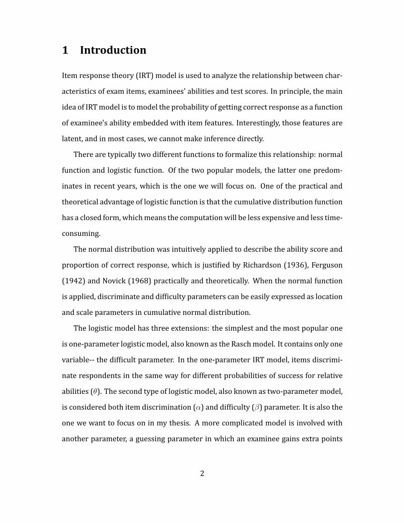
Item response theory (IRT) model is used to analyze the relationship between char-

acteristics of exam items, examinees' abilities and test scores. In principle, the main

idea of IRTmodel is tomodel the probability of getting correct response as a function

of examinee's ability embedded with item features. Interestingly, those features are

latent, and in most cases, we cannot make inference directly.

There are typically two different functions to formalize this relationship: normal

function and logistic function. Of the two popular models, the latter one predom-

inates in recent years, which is the one we will focus on. One of the practical and

theoretical advantage of logistic function is that the cumulative distribution function

has a closed form, whichmeans the computationwill be less expensive and less time-

consuming.

The normal distribution was intuitively applied to describe the ability score and

proportion of correct response, which is justi ied by Richardson (1936), Ferguson

(1942) and Novick (1968) practically and theoretically. When the normal function

is applied, discriminate and dif iculty parameters can be easily expressed as location

and scale parameters in cumulative normal distribution.

The logistic model has three extensions: the simplest and the most popular one

is one-parameter logisticmodel, also known as the Raschmodel. It contains only one

variable-- the dif icult parameter. In the one-parameter IRT model, items discrimi-

nate respondents in the same way for different probabilities of success for relative

abilities (θ). The second type of logistic model, also known as two-parameter model,

is considered both item discrimination (α) and dif iculty (β) parameter. It is also the

one we want to focus on in my thesis. A more complicated model is involved with

another parameter, a guessing parameter in which an examinee gains extra points

2

with successful guessing.

Traditional IRTmodel is divided into two families based on the kind of scored re-

sponse: dichotomous and polytomous. In contrast to polytomous IRTmodels, which

model the probability of selecting each response category, dichotomous IRT model

deals with the probability of selecting correct response.

In binary logistic IRT model,

yij | αj, βj, θi ∼ Bernoulli(

eαjθi−βj

1 + eαjθi−βj

), (1.1)

where yij = 1 if the ith student gets the jth problem correct and yij = 0 other-

wise. {αj; j = 1, 2, . . . , t} is the discrimination parameter which illustrates the in-

luence of students' ability on category propensity; {βj; j = 1, 2, . . . , t} is the loca-

tion parameter that re lects the dif iculty of jth item that does not depend on θi's;

{θi; i = 1, 2, . . . , n} is the individual ability for the ith respondent. In principle, α is

a scale parameter of abilities of individuals, therefore it is restricted to be positive.

It is highly related to the item's dif iculty value: under different levels of dif iculties,

discrimination parameters can be useful during different intervals of latent ability.

Typically, its value varies from 1/2 to 6.

The illustrated dataset is obtained from MA2611 Applied Statistics I-Test # 2.

This course, which is an introductory statistics course, aims to let students gain a

knowledge of basic statistical concepts, such as how to design and analyze experi-

ments and sampling studies and how to analyze data in an appropriate way. The test

we are going to analyze is the second test of this course. There are 17 questions, each

question has four options and one of them is correct. There are 101 students in this

class. After data screening and cleaning, the last question has two ambiguous an-

swers, while all of students got the last but one problem correct, so we exclude them

3

from further analysis.

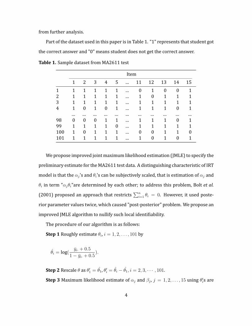
Part of the dataset used in this paper is in Table 1. "1" represents that student got

the correct answer and "0" means student does not get the correct answer.

Table 1. Sample dataset from MA2611 test

Item1 2 3 4 5 … 11 12 13 14 15

1 1 1 1 1 1 … 0 1 0 0 12 1 1 1 1 1 … 1 0 1 1 13 1 1 1 1 1 … 1 1 1 1 14 1 0 1 0 1 … 1 1 1 0 1

… … … … … … … … … … …98 0 0 0 1 1 … 1 1 1 0 199 1 1 1 1 0 … 1 1 1 1 1100 1 0 1 1 1 … 0 0 1 1 0101 1 1 1 1 1 … 1 0 1 0 1

Wepropose improved jointmaximum likelihood estimation (JMLE) to specify the

preliminary estimate for theMA2611 test data. A distinguishing characteristic of IRT

model is that the αj 's and θi's can be subjectively scaled, that is estimation of αj and

θi in term "αjθi"are determined by each other; to address this problem, Bolt et al.

(2001) proposed an approach that restricts ∑ni=1 θi = 0. However, it used poste-

rior parameter values twice, which caused "post-posterior" problem. We propose an

improved JMLE algorithm to nullify such local identi iability.

The procedure of our algorithm is as follows:

Step 1 Roughly estimate θi, i = 1, 2, . . . , 101 by

θi = log( yi· + 0.5

1− yi· + 0.5).

Step 2 Rescale θ as θ′1 = θ1, θ′i = θi − θ1, i = 2, 3, · · · , 101.

Step 3 Maximum likelihood estimate of αj and βj , j = 1, 2, . . . , 15 using θ′is are

4

obtained using the following likelihood function:

L(αj, βj | θ,y) =101∏i=1

e(αj θi−βj)yij

1 + eαj θi−βj

Step 4 Estimate θi using αj and βj with the restriction of θ1 = 0 by the same

likelihood function.

Step 5 Go back to step 3 and step 4 until it converged.

Maximum likelihood procedure for estimatingαj 's is L-BFGS-B proposed by Byrd

et al. (1995)with respect to thepositive restriction. It handles simplepredictorswith

respect to box constraints which allows us to give bounds on α. The main procedure

is to identify ixed and free variables at each step, and use only free ones to get higher

accuracy based on L-BFGS, while we omit the detail here.

It turns out that the algorithm for the 16th item does not converge. It is proba-

bly due to the fact that all of the students except one got this question correct, which

reveals that the question cannot discriminate students well and has relatively low

dif iculty. Therefore, we drop this question from further analysis. The values of es-

timation for α and β have been given in Table 2; for comparison, p is given to denote

the proportion of correct response for each item.

5

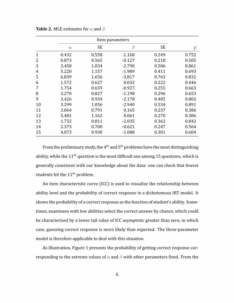
Table 2. MLE estimates for α and β

Item parametersα SE β SE p

1 0.432 0.558 -1.168 0.249 0.7522 0.873 0.565 -0.127 0.218 0.5053 3.458 1.034 -2.790 0.506 0.8614 5.220 1.157 -1.989 0.411 0.6935 6.839 1.656 -3.817 0.763 0.8326 1.572 0.627 0.032 0.222 0.4467 1.754 0.659 -0.927 0.255 0.6638 3.270 0.827 -1.198 0.296 0.6539 3.426 0.934 -2.178 0.405 0.80210 3.299 1.056 -2.940 0.534 0.89111 3.064 0.791 0.165 0.237 0.38612 5.481 1.162 0.061 0.270 0.38613 1.732 0.811 -2.035 0.362 0.84214 2.373 0.700 -0.621 0.247 0.56415 4.073 0.930 -1.088 0.301 0.604

From thepreliminary study, the 4th and5th problemshave themost distinguishing

ability, while the 11th question is themost dif icult one among 15 questions, which is

generally consistent with our knowledge about the data: one can check that fewest

students hit the 11th problem.

An item characteristic curve (ICC) is used to visualize the relationship between

ability level and the probability of correct response in a dichotomous IRT model. It

shows the probability of a correct response as the function of student's ability. Some-

times, examinees with low abilities select the correct answer by chance, which could

be characterized by a lower tail value of ICC asymptotic greater than zero; in which

case, guessing correct response is more likely than expected. The three-parameter

model is therefore applicable to deal with this situation.

As illustration, Figure 1 presents the probability of getting correct response cor-

responding to the extreme values of α and β with other parameters ixed. From the

6

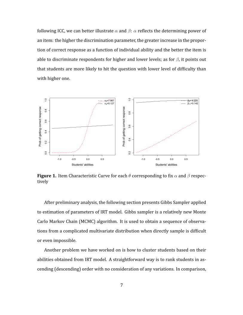
following ICC, we can better illustrate α and β: α re lects the determining power of

an item: the higher the discrimination parameter, the greater increase in the propor-

tion of correct response as a function of individual ability and the better the item is

able to discriminate respondents for higher and lower levels; as for β, it points out

that students are more likely to hit the question with lower level of dif iculty than

with higher one.

-1.0 -0.5 0.0 0.5

0.0

0.2

0.4

0.6

0.8

1.0

Students' abilities

Pro

b of

get

ting

corr

ect r

espo

nse

α5=7.867α2=0.127

-1.0 -0.5 0.0 0.5

0.2

0.4

0.6

0.8

1.0

Students' abilities

Pro

b of

get

ting

corr

ect r

espo

nse

β5=-4.225β11=0.142

Figure 1. Item Characteristic Curve for each θ corresponding to ix α and β respec-tively

After preliminary analysis, the following section presents Gibbs Sampler applied

to estimation of parameters of IRT model. Gibbs sampler is a relatively new Monte

Carlo Markov Chain (MCMC) algorithm. It is used to obtain a sequence of observa-

tions from a complicated multivariate distribution when directly sample is dif icult

or even impossible.

Another problem we have worked on is how to cluster students based on their

abilities obtained from IRT model. A straightforward way is to rank students in as-

cending (descending) order with no consideration of any variations. In comparison,

7

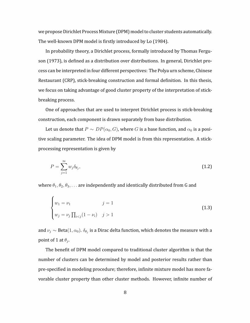
weproposeDirichlet ProcessMixture (DPM)model to cluster students automatically.

The well-known DPMmodel is irstly introduced by Lo (1984).

In probability theory, a Dirichlet process, formally introduced by Thomas Fergu-

son (1973), is de ined as a distribution over distributions. In general, Dirichlet pro-

cess can be interpreted in four different perspectives: The Polya urn scheme, Chinese

Restaurant (CRP), stick-breaking construction and formal de inition. In this thesis,

we focus on taking advantage of good cluster property of the interpretation of stick-

breaking process.

One of approaches that are used to interpret Dirichlet process is stick-breaking

construction, each component is drawn separately from base distribution.

Let us denote that P ∼ DP (α0, G), where G is a base function, and α0 is a posi-

tive scaling parameter. The idea of DPM model is from this representation. A stick-

processing representation is given by

P =∞∑j=1

wjδθj , (1.2)

where θ1, θ2, θ3, . . . are independently and identically distributed from G and

w1 = ν1 j = 1

wj = νj∏

i<j(1− νi) j > 1

(1.3)

and νj ∼ Beta(1, α0). δθj is a Dirac delta function, which denotes the measure with a

point of 1 at θj .

The bene it of DPM model compared to traditional cluster algorithm is that the

number of clusters can be determined by model and posterior results rather than

pre-speci ied in modeling procedure; therefore, in inite mixture model has more fa-

vorable cluster property than other cluster methods. However, in inite number of

8

components cause complicated algorithms and computations. Walker et al. (2011)

introduced two latent variables to decide which components should be considered

when processing Monte Carlo Markov Chain (MCMC) method.

In the rest of this paper we will discuss (1) parameters are estimated through

Monte Carlo Markov chain method with ARS algorithm; (2) various model checking

approaches will be discussed, including traceplots, autocorrelation, goodness-of- it

test and predictive test; (3) cluster students' abilities by DPM model with improved

slice sampling method. The ideal output is to guide the instructor to grade students

basedondifferent levels of students' ability rather thanonly theproportionof correct

responses.

2 Bayesian Estimation with MCMCMethod

2.1 Speci ication of Model Parameter

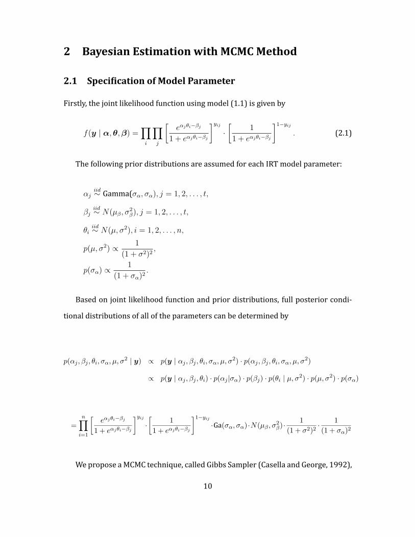
Firstly, the joint likelihood function using model (1.1) is given by

f(y | α,θ,β) =∏i

∏j

[eαjθi−βj

1 + eαjθi−βj

]yij·[

1

1 + eαjθi−βj

]1−yij

. (2.1)

The following prior distributions are assumed for each IRT model parameter:

αjiid∼ Gamma(σα, σα), j = 1, 2, . . . , t,

βjiid∼ N(µβ, σ

2β), j = 1, 2, . . . , t,

θiiid∼ N(µ, σ2), i = 1, 2, . . . , n,

p(µ, σ2) ∝ 1

(1 + σ2)2,

p(σα) ∝1

(1 + σα)2.

Based on joint likelihood function and prior distributions, full posterior condi-

tional distributions of all of the parameters can be determined by

p(αj , βj , θi, σα, µ, σ2 | y) ∝ p(y | αj , βj , θi, σα, µ, σ

2) · p(αj , βj , θi, σα, µ, σ2)

∝ p(y | αj , βj , θi) · p(αj |σα) · p(βj) · p(θi | µ, σ2) · p(µ, σ2) · p(σα)

=n∏

i=1

[eαjθi−βj

1 + eαjθi−βj

]yij·[

1

1 + eαjθi−βj

]1−yij

·Ga(σα, σα)·N(µβ, σ2β)·

1

(1 + σ2)2· 1

(1 + σα)2

Wepropose aMCMC technique, called Gibbs Sampler (Casella and George, 1992),

10

tomake inference of IRTmodel. The Gibbs Sampler generates a random sample from

{x1, x2, . . . , xn} from the joint distribution p(x1, x2, . . . , xn) as follows:

1. Let {x(0)1 , x

(0)2 , . . . , x

(0)n } be starting values.

2. Drawx(j)i fromconditiondistributionp(xi|x(j)

1 , . . . , x(j)i−1, x

(j−1)i+1 , . . . , x

(j−1)n ). That

is, draw each variable from the conditional distribution the most recent values

and updating the variable with its new value after it has been sampled.

After a large number,B, of iterations, we obtain {x(B)1 , x

(B)2 , . . . , x

(B)n }.

It is noted that we assume αj follows a gamma distribution, which is different

from "normal distribution" in popular researches. The reason is that it is ensured

the mean of αj always equal to 1, so the inference will not be affected by its neighbor

θi.

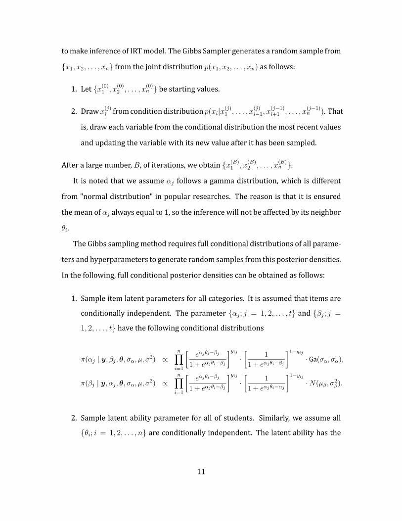
The Gibbs sampling method requires full conditional distributions of all parame-

ters and hyperparameters to generate random samples from this posterior densities.

In the following, full conditional posterior densities can be obtained as follows:

1. Sample item latent parameters for all categories. It is assumed that items areconditionally independent. The parameter {αj; j = 1, 2, . . . , t} and {βj; j =

1, 2, . . . , t} have the following conditional distributions

π(αj | y, βj ,θ, σα, µ, σ2) ∝n∏

i=1

[eαjθi−βj

1 + eαjθi−βj

]yij·[

1

1 + eαjθi−βj

]1−yij

· Ga(σα, σα),

π(βj | y, αj ,θ, σα, µ, σ2) ∝

n∏i=1

[eαjθi−βj

1 + eαjθi−βj

]yij·[

1

1 + eαjθi−αj

]1−yij

·N(µβ, σ2β).

2. Sample latent ability parameter for all of students. Similarly, we assume all{θi; i = 1, 2, . . . , n} are conditionally independent. The latent ability has the

11

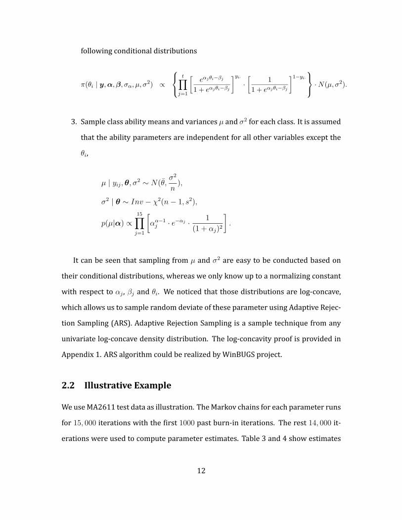
following conditional distributions

π(θi | y,α,β, σα, µ, σ2) ∝

t∏

j=1

[eαjθi−βj

1 + eαjθi−βj

]yi··[

1

1 + eαjθi−βj

]1−yi·

·N(µ, σ2).

3. Sample class ability means and variances µ and σ2 for each class. It is assumed

that the ability parameters are independent for all other variables except the

θi,

µ | yij,θ, σ2 ∼ N(θ,σ2

n),

σ2 | θ ∼ Inv − χ2(n− 1, s2),

p(µ|α) ∝15∏j=1

[αα−1j · e−αj · 1

(1 + αj)2

].

It can be seen that sampling from µ and σ2 are easy to be conducted based on

their conditional distributions, whereas we only know up to a normalizing constant

with respect to αj , βj and θi. We noticed that those distributions are log-concave,

which allows us to sample random deviate of these parameter using Adaptive Rejec-

tion Sampling (ARS). Adaptive Rejection Sampling is a sample technique from any

univariate log-concave density distribution. The log-concavity proof is provided in

Appendix 1. ARS algorithm could be realized by WinBUGS project.

2.2 Illustrative Example

WeuseMA2611 test data as illustration. TheMarkov chains for each parameter runs

for 15, 000 iterations with the irst 1000 past burn-in iterations. The rest 14, 000 it-

erations were used to compute parameter estimates. Table 3 and 4 show estimates

12

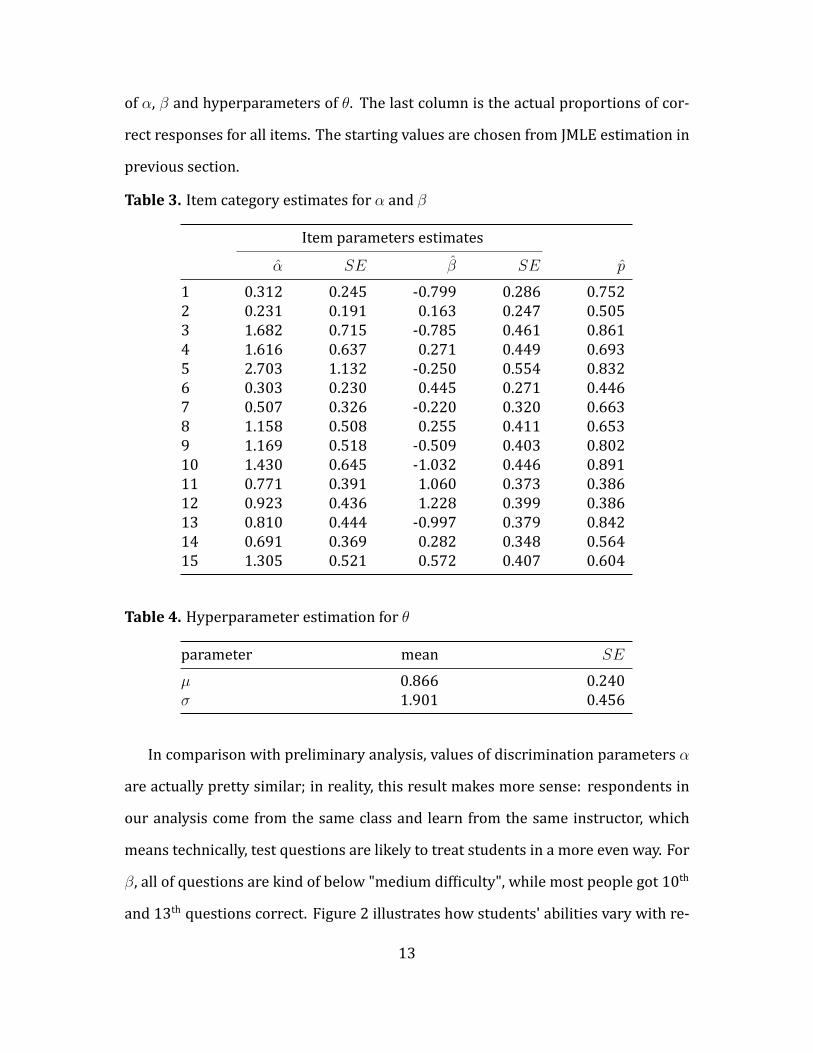
of α, β and hyperparameters of θ. The last column is the actual proportions of cor-

rect responses for all items. The starting values are chosen from JMLE estimation in

previous section.

Table 3. Item category estimates for α and β

Item parameters estimatesα SE β SE p

1 0.312 0.245 -0.799 0.286 0.7522 0.231 0.191 0.163 0.247 0.5053 1.682 0.715 -0.785 0.461 0.8614 1.616 0.637 0.271 0.449 0.6935 2.703 1.132 -0.250 0.554 0.8326 0.303 0.230 0.445 0.271 0.4467 0.507 0.326 -0.220 0.320 0.6638 1.158 0.508 0.255 0.411 0.6539 1.169 0.518 -0.509 0.403 0.80210 1.430 0.645 -1.032 0.446 0.89111 0.771 0.391 1.060 0.373 0.38612 0.923 0.436 1.228 0.399 0.38613 0.810 0.444 -0.997 0.379 0.84214 0.691 0.369 0.282 0.348 0.56415 1.305 0.521 0.572 0.407 0.604

Table 4. Hyperparameter estimation for θ

parameter mean SE

µ 0.866 0.240σ 1.901 0.456

In comparison with preliminary analysis, values of discrimination parameters α

are actually pretty similar; in reality, this result makes more sense: respondents in

our analysis come from the same class and learn from the same instructor, which

means technically, test questions are likely to treat students in a more even way. For

β, all of questions are kind of below "medium dif iculty", while most people got 10th

and 13th questions correct. Figure 2 illustrates how students' abilities vary with re-

13

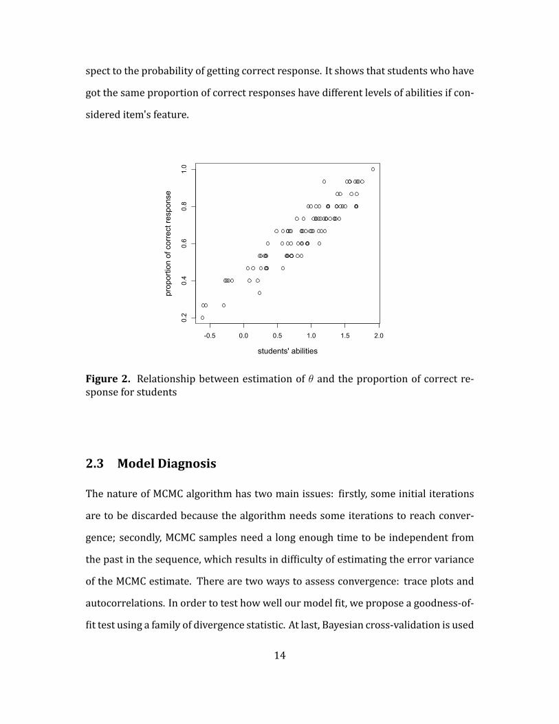
spect to the probability of getting correct response. It shows that students who have

got the same proportion of correct responses have different levels of abilities if con-

sidered item's feature.

-0.5 0.0 0.5 1.0 1.5 2.0

0.2

0.4

0.6

0.8

1.0

students' abilities

prop

ortio

n of

cor

rect

resp

onse

Figure 2. Relationship between estimation of θ and the proportion of correct re-sponse for students

2.3 Model Diagnosis

The nature of MCMC algorithm has two main issues: irstly, some initial iterations

are to be discarded because the algorithm needs some iterations to reach conver-

gence; secondly, MCMC samples need a long enough time to be independent from

the past in the sequence, which results in dif iculty of estimating the error variance

of the MCMC estimate. There are two ways to assess convergence: trace plots and

autocorrelations. In order to test how well our model it, we propose a goodness-of-

it test using a family of divergence statistic. At last, Bayesian cross-validation is used

14

to examine the predictive ability of our model in view of both items and individuals.

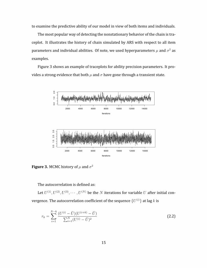
Themost popular way of detecting the nonstationary behavior of the chain is tra-

ceplot. It illustrates the history of chain simulated by ARS with respect to all item

parameters and individual abilities. Of note, we used hyperparameters µ and σ2 as

examples.

Figure 3 shows an example of traceplots for ability precision parameters. It pro-

vides a strong evidence that both µ and σ have gone through a transient state.

2000 4000 6000 8000 10000 12000 14000

0.0

1.0

2.0

Iterations

2000 4000 6000 8000 10000 12000 14000

0.5

1.5

2.5

3.5

Iterations

Figure 3. MCMC history of µ and σ2

The autocorrelation is de ined as:

Let U (1), U (2), U (3), · · · , U (N) be the N iterations for variable U after initial con-

vergence. The autocorrelation coef icient of the sequence {U (i)} at lag k is

rk =N−k∑i=1

(U (i) − U)(U (i+k) − U)∑Ni=1(U

(i) − U)2(2.2)

15

where U = N−1∑N

i=1 U(i), and its asymptomatic standarderror is stek =

{N − k

N(N + 2)

}1/2

.

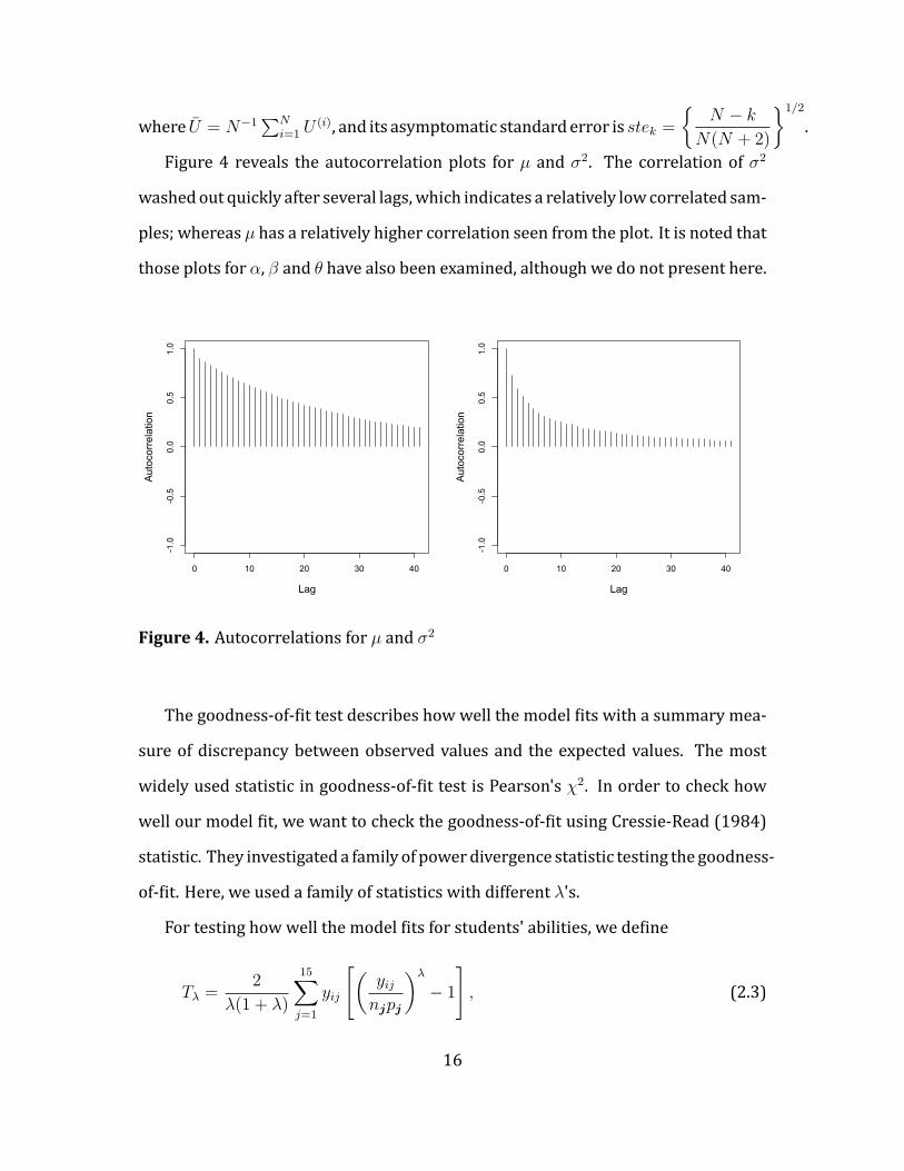
Figure 4 reveals the autocorrelation plots for µ and σ2. The correlation of σ2

washedout quickly after several lags, which indicates a relatively lowcorrelated sam-

ples; whereas µ has a relatively higher correlation seen from the plot. It is noted that

those plots for α, β and θ have also been examined, although we do not present here.

0 10 20 30 40

-1.0

-0.5

0.0

0.5

1.0

Lag

Autocorrelation

0 10 20 30 40

-1.0

-0.5

0.0

0.5

1.0

Lag

Autocorrelation

Figure 4. Autocorrelations for µ and σ2

The goodness-of- it test describes how well the model its with a summary mea-

sure of discrepancy between observed values and the expected values. The most

widely used statistic in goodness-of- it test is Pearson's χ2. In order to check how

well our model it, we want to check the goodness-of- it using Cressie-Read (1984)

statistic. They investigateda family of powerdivergence statistic testing thegoodness-

of- it. Here, we used a family of statistics with different λ's.

For testing how well the model its for students' abilities, we de ine

Tλ =2

λ(1 + λ)

15∑j=1

yij

[(yijnjpj

)λ

− 1

], (2.3)

16

where yij is the observed number of correct response and njpj is the expected num-

ber, which is approximated by E(T =∑

i yij). The special cases are likelihood ratio

statistic (λ = −1) and Pearson's χ2 statistic (λ = −2).

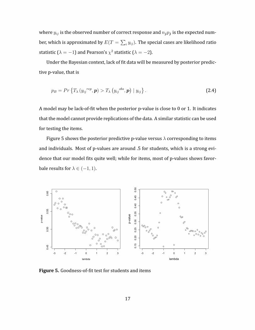
Under the Bayesian context, lack of it data will be measured by posterior predic-

tive p-value, that is

pB = Pr{Tλ (yij

rep,p) > Tλ

(yij

obs,p)| yij

}. (2.4)

A model may be lack-of- it when the posterior p-value is close to 0 or 1. It indicates

that themodel cannot provide replications of the data. A similar statistic can be used

for testing the items.

Figure 5 shows the posterior predictive p-value versus λ corresponding to items

and individuals. Most of p-values are around .5 for students, which is a strong evi-

dence that our model its quite well; while for items, most of p-values shows favor-

bale results for λ ∈ (−1, 1).

-3 -2 -1 0 1 2 3

0.45

0.50

0.55

0.60

lambda

p-value

-3 -2 -1 0 1 2 3

0.15

0.20

0.25

0.30

0.35

0.40

0.45

0.50

lambda

p-value

Figure 5. Goodness-of- it test for students and items

17

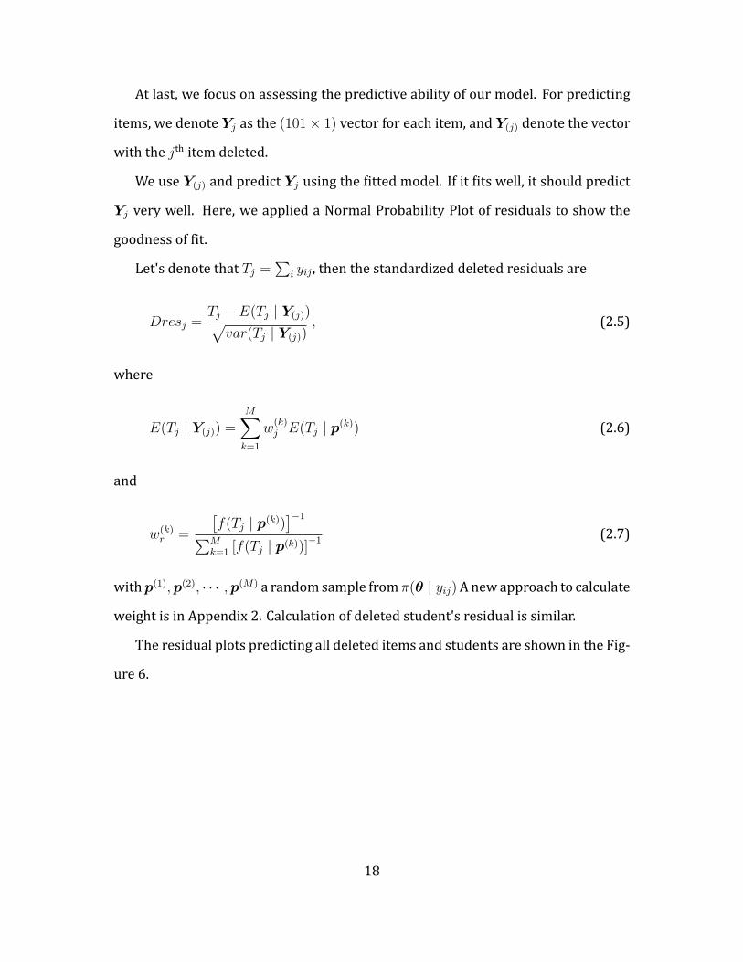
At last, we focus on assessing the predictive ability of our model. For predicting

items, we denote Yj as the (101× 1) vector for each item, and Y(j) denote the vector

with the jth item deleted.

We use Y(j) and predict Yj using the itted model. If it its well, it should predict

Yj very well. Here, we applied a Normal Probability Plot of residuals to show the

goodness of it.

Let's denote that Tj =∑

i yij , then the standardized deleted residuals are

Dresj =Tj − E(Tj | Y(j))√

var(Tj | Y(j)), (2.5)

where

E(Tj | Y(j)) =M∑k=1

w(k)j E(Tj | p(k)) (2.6)

and

w(k)r =

[f(Tj | p(k))

]−1∑Mk=1 [f(Tj | p(k))]

−1 (2.7)

withp(1),p(2), · · · ,p(M) a randomsample fromπ(θ | yij)Anewapproach to calculate

weight is in Appendix 2. Calculation of deleted student's residual is similar.

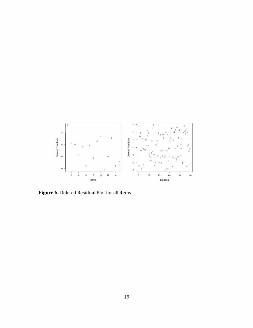
The residual plots predicting all deleted items and students are shown in the Fig-

ure 6.

18

2 4 6 8 10 12 14

-2-1

01

Items

Del

eted

Res

idua

ls

0 20 40 60 80 100

-3-2

-10

12

3

Students

Del

eted

Res

idua

ls

Figure 6. Deleted Residual Plot for all items

19

3 Dirichlet Process Mixture Model

3.1 Introduction

Dirichlet process mixture (DPM) model is irstly introduced by Lo(1984) with the

Gaussian kernel

fP (y) =

∫N(y; θ)dP (θ), (3.1)

where P ∼ DP (α0, G) and θ = (µ, σ2). With inspiration of stick-processing repre-

sentation, we can write an in inite-dimensional mixture model, whose each compo-

nent is drawn separately from base distribution, that is:

fθ,w(y) =∞∑j=1

wj · p(y; θj|α,β), (3.2)

where

p(y; θj|α,β) =t∏

m=1

[eαmθj−βm

1 + eαmθj−βm

]y·m·[

1

1 + eαmθj−βm

]1−y·m

. (3.3)

Our purpose is to implement Gibbs sampler in this joint likelihood function; how-

ever, it is quite dif icult to sample in inite number of θj 's to proceed algorithm.

Walker et al. (2011) proposed a new sampler method for sampling the DPM

model. This approach introduces two latent variables which make inite number of

mixtures, which tried to avoid such dif iculties. The key idea of slice sampler is to

introduce a latent variable u that help to sample from a inite number of θj 's. After

given u, the number of partitions becomes inite:

20

fθ,w(y, u) =∞∑j=1

1(u < wj) · p(y; θj|α,β). (3.4)

When given u, the indices are reduced toAu = {j : wj > u}. After making a inite

sum, a further latent variable, d, will be introduced. It indicates which component

attribute to the density function, with which trick we can get rid of summation sign:

fθ,w(y, u, d) = 1(u < wd) · p(y; θj|α,β), (3.5)

where w is de ined in (1.3).

Although this formof distribution could be easily handledbyGibbs Sampler, there

are some limitations that will cost extra works. When proceeding Gibbs sampling,

updating uwill cause the change of the set ∪ni=1A(ui) and consequently lead to more

simulation of w's.

To overcome this problem,we can ixw's in the generation ofu. Therefore, amore

general form had been proposed:

fν,θ(y, u, d) = ξ−1d 1(u < ξd)wdp(y; θ|α,β), (3.6)

where ξ1, ξ2, ξ3, . . . is any positive sequence. The choice of this sequence is anotherissue thatwewill not discuss here. Here,we consider the sequence as ξj = (1−k)kj−1

where k = 0.5. The joint likelihood function is de ined by

Lw,θ({yi, ui, di = ki}101i=1) =

n∏i=1

fν,θ(yi, ui, di) =

n∏i=1

{ξ−1di

1(ui < ξdi)wdip(yi; θj |α,β)}. (3.7)

21

The prior distributions are de ined

θj ∼ N(µ, σ2),

p(µ, σ2) ∝ 1

(1 + σ2)2,

νj ∼ Beta(1, α0).

3.2 Sampling Algorithm

In this section, we are going to implement Gibbs Sampling for the proposed density

distribution. Thevariables that need tobe sampledare{(θj, νj), j = 1, 2, . . . ; (di, ui), i =

1, 2, 3, . . . , n; (µ, σ2)}.

1. We begin with sample the latent variable ui which is also the simplest one. The

condition posterior distribution is

π(ui| · · · ) ∝ 1(0 < ui < ξdi).

2. Then, we sample the weight of mixture model νj . Based on the joint likelihood

distribution (3.8), the conditional distribution of νj is given by

π(νj| · · · ) ∝ Beta(aj, bj),

where aj = 1 +∑n

i=1 1(di = j) and bj = α0 +∑n

i=1 1(di > j), and hence we

can calculate wj 's.

3. We will sample individual abilities θj in this step. The posterior conditional

22

distribution is as follows:

f(θj| · · · ) ∝ N(µ, σ2)∏di=j

p(yi; θj|α,β),

when there is no {ki = j}, then

θj| · · · ∼ N(µ, σ2).

4. Then we will sample the indicator variables di. It is given by

p(di = k| · · · ) ∝ 1(k : ξk > ui)wk/ξkN(yi; θk).

5. At last, the posterior conditional distribution for α0 is

π(α0|d, · · · ) ∝ αd0Γ(α0)π(α0)/Γ(α0 + n),

where d is the number of distinct ki's, that is the number of clusters. We will

present it will be a nice way to sample from the posterior distribution when

prior distribution of α0 is a gamma distribution. Suppose α0 ∼ Gamma(a, b),

then we can deduce

π(α0|d, · · · ) ∝ π(α0)αd−10 (α0 + n)B(α0 + 1, n)

∝ π(α0)αd−10 (α0 + n)

∫ 1

0

xα0(1− x)n−1dx,

π(α0|d, · · · ) can be the marginal distribution of the following distribution:

π(α0|d, η, · · · ) ∝ π(α0)α0d−1(α0 + n)ηα0(1− η)n−1,

23

where α > 0 and 0 < η < 1. After simple algebra, the posterior distribution of

α0 reduces to the mixture of two gamma distributions,

π(α0|d, η, · · · )πηG(a+ d, b− log(η)) + (1− πη)G(a+ d− 1, b− log(η)),

where πη/(1− πη) = (a+ d− 1)/[n(b− log(η))]. Second,

π(η|α0, d) ∝ ηα0(1− η)n−1,

that is, posterior distribution of η follows a beta distribution with mean (α0 +

1)/(α0 + n+ 1).

After obtaining d and α0 during each iteration, draw η from beta distribution

and then updateα0 from themixture gammadistributions using ARS algorithm

(log-concavity proved). Since µ and σ2 only depend on θ, their posterior distri-

butions are as the same as in section 2.3.

To succeed proceeding algorithm, we need to sample enough θj 's. The principle

to ind required set of k is k = {1, 2, . . . , N}, N = maxi{Ni}, whereN is the largest

integer l for which ξl > ui.

3.3 Application of DPMModel into MA2611 Test Data

In this section, of interest is to cluster students based on different ability levels. To

initialize di's, the students' abilities were split into 10 equal clusters according to

ascending order. Student's ability parameter θi with µ and σ2 will be the only pa-

rameter when directly retrieved values of discrimination and dif iculty parameter

in Section 2.2. The Gibbs Sampler ran for 5000 iterations with the irst 500 burn-in

samples. Figure 7 shows the running average of number clusters, it is clear that 5000

24

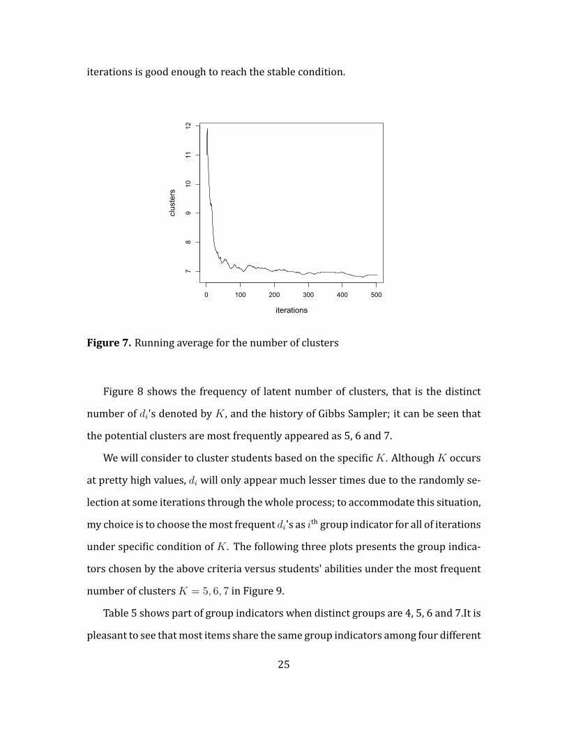
iterations is good enough to reach the stable condition.

0 100 200 300 400 500

78

910

1112

iterations

clusters

Figure 7. Running average for the number of clusters

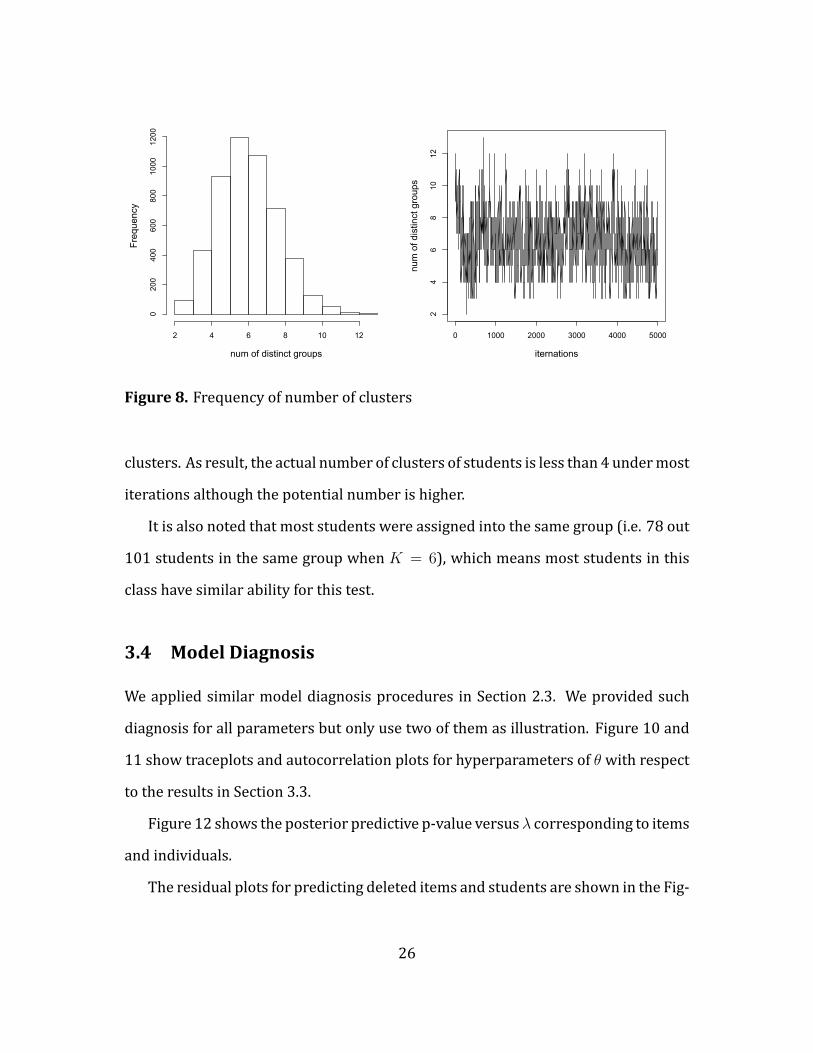
Figure 8 shows the frequency of latent number of clusters, that is the distinct

number of di's denoted by K , and the history of Gibbs Sampler; it can be seen that

the potential clusters are most frequently appeared as 5, 6 and 7.

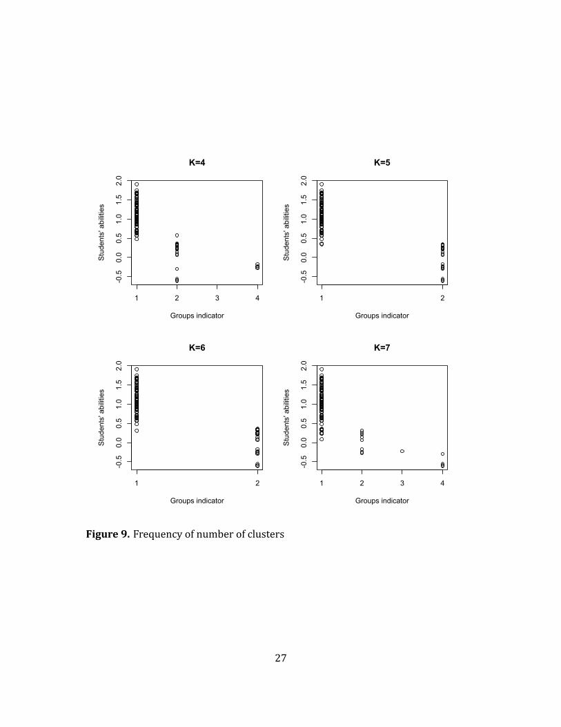
We will consider to cluster students based on the speci icK . AlthoughK occurs

at pretty high values, di will only appear much lesser times due to the randomly se-

lection at some iterations through thewhole process; to accommodate this situation,

my choice is to choose themost frequent di's as ith group indicator for all of iterations

under speci ic condition of K . The following three plots presents the group indica-

tors chosen by the above criteria versus students' abilities under the most frequent

number of clustersK = 5, 6, 7 in Figure 9.

Table 5 shows part of group indicators when distinct groups are 4, 5, 6 and 7.It is

pleasant to see thatmost items share the same group indicators among four different

25

num of distinct groups

Frequency

2 4 6 8 10 12

0200

400

600

800

1000

1200

0 1000 2000 3000 4000 5000

24

68

1012

iternations

num

of d

istin

ct g

roup

sFigure 8. Frequency of number of clusters

clusters. As result, the actual number of clusters of students is less than 4 undermost

iterations although the potential number is higher.

It is also noted that most students were assigned into the same group (i.e. 78 out

101 students in the same group when K = 6), which means most students in this

class have similar ability for this test.

3.4 Model Diagnosis

We applied similar model diagnosis procedures in Section 2.3. We provided such

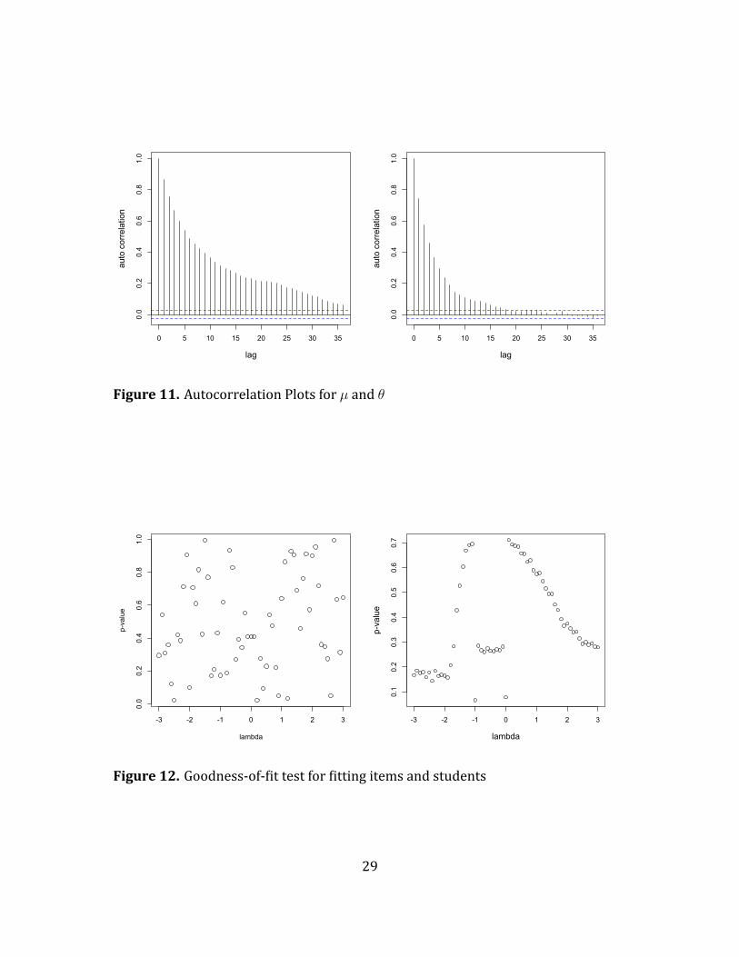
diagnosis for all parameters but only use two of them as illustration. Figure 10 and

11 show traceplots and autocorrelation plots for hyperparameters of θ with respect

to the results in Section 3.3.

Figure 12 shows the posterior predictive p-value versusλ corresponding to items

and individuals.

The residual plots for predicting deleted items and students are shown in the Fig-

26

-0.5

0.0

0.5

1.0

1.5

2.0

K=4

Groups indicator

Stu

dent

s' a

bilit

ies

1 2 3 4-0.5

0.0

0.5

1.0

1.5

2.0

K=5

Groups indicator

Stu

dent

s' a

bilit

ies

1 2

-0.5

0.0

0.5

1.0

1.5

2.0

K=6

Groups indicator

Stu

dent

s' a

bilit

ies

1 2

-0.5

0.0

0.5

1.0

1.5

2.0

K=7

Groups indicator

Stu

dent

s' a

bilit

ies

1 2 3 4

Figure 9. Frequency of number of clusters

27

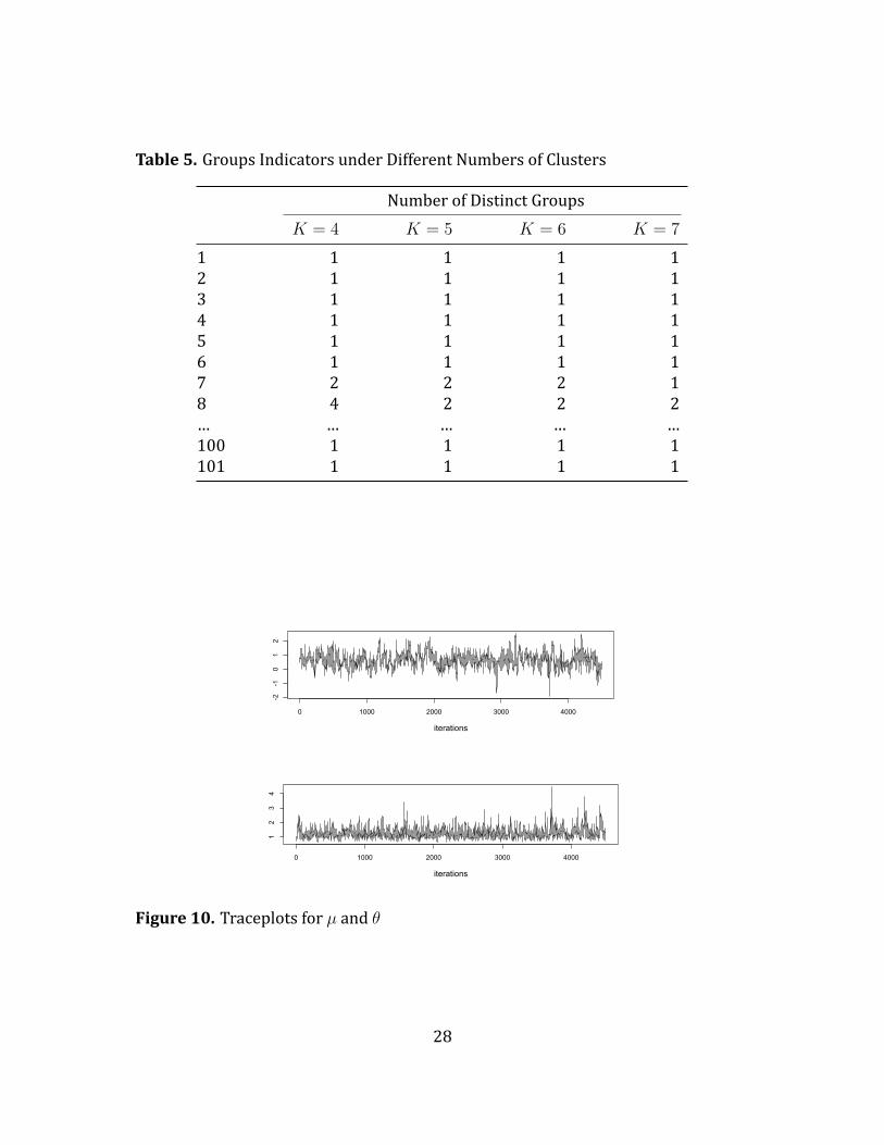
Table 5. Groups Indicators under Different Numbers of Clusters

Number of Distinct GroupsK = 4 K = 5 K = 6 K = 7

1 1 1 1 12 1 1 1 13 1 1 1 14 1 1 1 15 1 1 1 16 1 1 1 17 2 2 2 18 4 2 2 2… … … … …100 1 1 1 1101 1 1 1 1

0 1000 2000 3000 4000

-2-1

01

2

iterations

0 1000 2000 3000 4000

12

34

iterations

Figure 10. Traceplots for µ and θ

28

0 5 10 15 20 25 30 35

0.0

0.2

0.4

0.6

0.8

1.0

lag

auto

cor

rela

tion

0 5 10 15 20 25 30 35

0.0

0.2

0.4

0.6

0.8

1.0

lag

auto

cor

rela

tion

Figure 11. Autocorrelation Plots for µ and θ

-3 -2 -1 0 1 2 3

0.0

0.2

0.4

0.6

0.8

1.0

lambda

p-value

-3 -2 -1 0 1 2 3

0.1

0.2

0.3

0.4

0.5

0.6

0.7

lambda

p-value

Figure 12. Goodness-of- it test for itting items and students

29

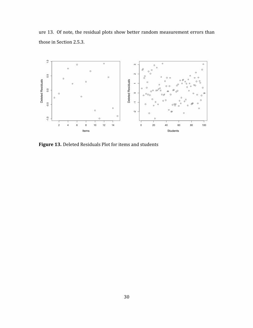
ure 13. Of note, the residual plots show better random measurement errors than

those in Section 2.5.3.

2 4 6 8 10 12 14

-1.0

-0.5

0.0

0.5

1.0

Items

Del

eted

Res

idua

ls

0 20 40 60 80 100

-2-1

01

23

StudentsD

elet

ed R

esid

uals

Figure 13. Deleted Residuals Plot for items and students

30

4 Conclusion

We have discussed binary Item Response Theory model and Dirichlet process mix-

ture (DPM) model. We have applied both models to MA2611 test # 2, Spring 2012,

and as an illustration, severalmodel diagnosis procedures followed. The primary ob-

jective is to discuss two-parameter IRT model of dichotomous response and cluster

students automaticallywith DPMmodel. It is highly recommended to grade students

in this way, since both student's ability and item's features are taken into considera-

tion, instead of just the proportion of correct responses. Firstly, we have provided a

Markov chain Monte Carlo (MCMC)method with Adaptive Rejection Sampling (ARS)

to estimate parameters. Using this method, we found that students' abilities were

consistent with the number of correct responses they got. Two improved model

checking procedures have been proposed. Except for traditional traceplots and auto-

correlation, a family of divergence statistics, Cressie-Read statistic, was used to test

the goodness-of- it of our model. The evidence of goodness-of- it therefore becomes

stronger.

DPM model has good property of clustering, since we do not have to decide spe-

ci ic number of clusters in advance compared to a inite mixture model. However,

in inite discrete components from a random distribution can cause expensive com-

putation. Toovercome this issue, slice sampling algorithm introduces two latent vari-

ables to determine which components are required to be sampled, which results in

a pretty simple easy and simple formation, see Kalli et al. (2011).

By building similar full conditional distributions, we implemented students' abil-

ities obtained from IRT model into DPM model. Potential number of clusters were

then obtained that mostly occurred with sizes 5, 6 and 7. The inal decision is based

on the expertise of the instructors.

31

Future work will focus on how to grade students more precisely. Speci ically, us-

ing the Gibbs sampler, "who belongs towhich group" still remains an issue due to the

nature of MCMC although we can obtain potential number of clusters. In which case,

students can be graded with uncertainty; that is, student A can be possibly graded

with student B who, however has lower ability. To accommodate this lexibility, an

instructor may consider combining our result with in-class performance and subjec-

tive impression when grading.

32

A Appendix

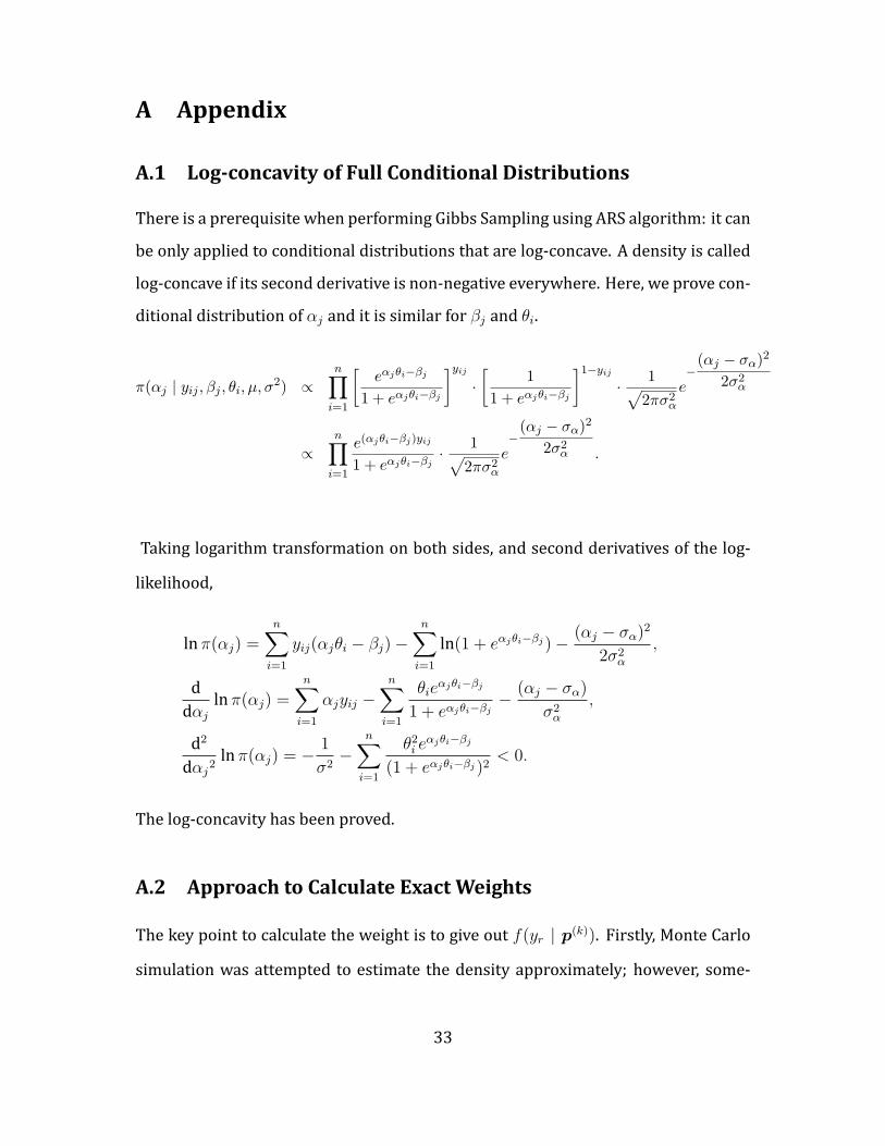
A.1 Log-concavity of Full Conditional Distributions

There is a prerequisite when performing Gibbs Sampling using ARS algorithm: it canbe only applied to conditional distributions that are log-concave. A density is calledlog-concave if its second derivative is non-negative everywhere. Here, we prove con-ditional distribution of αj and it is similar for βj and θi.

π(αj | yij , βj , θi, µ, σ2) ∝n∏

i=1

[eαjθi−βj

1 + eαjθi−βj

]yij·[

1

1 + eαjθi−βj

]1−yij

· 1√2πσ2

α

e−(αj − σα)

2

2σ2α

∝n∏

i=1

e(αjθi−βj)yij

1 + eαjθi−βj· 1√

2πσ2α

e−(αj − σα)

2

2σ2α .

Taking logarithm transformation on both sides, and second derivatives of the log-

likelihood,

ln π(αj) =n∑

i=1

yij(αjθi − βj)−n∑

i=1

ln(1 + eαjθi−βj)− (αj − σα)2

2σ2α

,

ddαj

ln π(αj) =n∑

i=1

αjyij −n∑

i=1

θieαjθi−βj

1 + eαjθi−βj− (αj − σα)

σ2α

,

d2

dαj2ln π(αj) = − 1

σ2−

n∑i=1

θ2i eαjθi−βj

(1 + eαjθi−βj)2< 0.

The log-concavity has been proved.

A.2 Approach to Calculate Exact Weights

The key point to calculate the weight is to give out f(yr | p(k)). Firstly, Monte Carlo

simulation was attempted to estimate the density approximately; however, some-

33

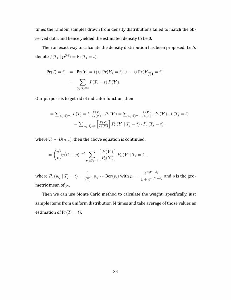
times the random samples drawn from density distributions failed to match the ob-

served data, and hence yielded the estimated density to be 0.

Then an exact way to calculate the density distribution has been proposed. Let's

denote f(Tj | p(k)) = Pr(Tj = t),

Pr(Ti = t) = Pr(Y1 = t) ∪ Pr(Y2 = t) ∪ · · · ∪ Pr(Y(nt) = t)

=∑

yij :Tj=t

I (Ti = t)P (Y ).

Our purpose is to get rid of indicator function, then

=∑

yij :Tj=t I (Tj = t) P (Y )Pe(Y )

· Pe(Y ) =∑

yij :Tj=t ·P (Y )Pe(Y )

· Pe(Y ) · I (Tj = t)

=∑

yij :Tj=t

[P (Y )Pe(Y )

]Pe (Y | Tj = t) · Pe (Tj = t) ,

where Tj ∼ B(n, t), then the above equation is continued:

=

(n

t

)pt(1− p)n−t

∑yij :Tj=t

[P (Y )

Pe(Y )

]Pe (Y | Tj = t) ,

where Pe (yij | Tj = t) =1(nt

) , yij ∼ Ber(pi) with pi =eαjθi−βj

1 + eαjθi−βjand p is the geo-

metric mean of pi.

Then we can use Monte Carlo method to calculate the weight; speci ically, just

sample items from uniform distribution M times and take average of those values as

estimation of Pr(Ti = t).

34

References

[1] Daniel M. Bolt, Allan S. Cohen and James A. Wollack. A Mixture Item Response

Model for Multiple-Choice Data. Journal of Educational and Behavioral Statistics,

Vol. 26, No. 4 (2001), pp. 381-409.

[2] Jean-Paul Fox. Bayesian Item Response Modeling: Theory and Application.

Springer, 2010.

[3] Kei Myazakli and Takahiro Hoshino. A Bayesian Semiparametric Item Response

Modelwith Dirichlet Process Priors. Psychometria, Vol. 74, N0. 3 (2009), pp. 375-

393.

[4] Leo A. Goodman. Exploratory Latent Structure Analysis Using Both Identi iable

and Unidenti iable Models. Biometrika, Vol. 61, No.2 (1974), pp. 215-231.

[5] Maria Kalli, Jim E. Grif in and Stephen G. Walker. Slice sampling mixture models.

Statistics and Computing, Vol. 21, No. 1 (2009), pp. 93-105.

[6] Michael D. Escobar and Mike West. Bayesian Density Estimation and Inference

using Mixtures. Journal of the American Statistical Association, Vol. 90, No. 430

(1995), pp. 577-588.

[7] Noel Cressie and Timothy R.C. Read. Multinomial Goodness-of-Fit Tests. Journal

of the Royal Statistical Society. Series B (Methodological), Vol. 46, No.3 (1984), pp.

440-464.

[8] Stephen G. Walker. Sampling Dirichlet Mixture Model with Slices. Communica-

tions in Statistics--Simulation and Computation, Vol. 36, No.1 (2007), pp. 45-54.

35

[9] W. R. Gilks and P. Wild. Adaptive Rejection Sampling for Gibbs Sampling. Journal

of the Royal Statistical Society. Series C (Applied Statistics), Vol. 41, No. 2 (1992),

pp. 337-348.

36