Aalborg Universitet

Wave propagation in non-uniform waveguides

Nielsen, Rasmus Bruus

Publication date:2015

Document VersionEarly version, also known as pre-print

Link to publication from Aalborg University

Citation for published version (APA):Nielsen, R. B. (2015). Wave propagation in non-uniform waveguides. Institut for Mekanik og Produktion, AalborgUniversitet.

General rightsCopyright and moral rights for the publications made accessible in the public portal are retained by the authors and/or other copyright ownersand it is a condition of accessing publications that users recognise and abide by the legal requirements associated with these rights.

? Users may download and print one copy of any publication from the public portal for the purpose of private study or research. ? You may not further distribute the material or use it for any profit-making activity or commercial gain ? You may freely distribute the URL identifying the publication in the public portal ?

Take down policyIf you believe that this document breaches copyright please contact us at vbn@aub.aau.dk providing details, and we will remove access tothe work immediately and investigate your claim.

Downloaded from vbn.aau.dk on: April 30, 2017

Department of Mechanical and Manufacturing Engineering

Aalborg University, Denmark.

Wave propagation in non-uniformwaveguides

Ph.D. Thesis

by

Rasmus Bruus Nielsen

Department of Mechanical and Manufacturing Engineering, Aalborg UniversityFibigerstraede 16, DK-9220 Aalborg East, Denmark

e-mail: rn@m-tech.aau.dk

PREPRINT – April 11, 2015

Copyright c© 2015 Rasmus Bruus Nielsen

This report, or parts of it, except the attached papers may be reproducedwithout the permission of the author, provided that due reference is given.Questions and comments are most welcome and may be directed to the author

ISBN 87-91200-78-4

i

ii

Preface

This thesis has been submitted to the Faculty of Engineering and Science atAalborg University in partial fulfilment of the requirements for the degree ofDoctor of Philosophy in Mechanical Engineering. The underlying work hasbeen carried out at the Department of Mechanical and Manufacturing Engi-neering, Aalborg University, during the period from September 2011 to De-cember 2014. The work is a part of the research project entitled ”AdvancedModelling of Wave Propagation in Spatially Curved Elastic Rods and Pipes”supported by the The Danish Council for Independent Research, Technologyand Production Sciences (FTP) grant number UK 95 OS63822 PO83004. Thefinancial support from FTP is gratefully acknowledged.

The project has been supervised by Professor, Ph.D., Dr. Sci., Sergey V.Sorokin to whom I owe my sincere gratitude. The endless number of discus-sions, hours of debugging, constructive criticism given to manuscripts, and thealways enthusiastic attitude towards the work has been an absolutely essen-tial support. A special thanks is addressed to Professor Nigel Peake and theWaves Group at Department of Applied Mathematics and Theoretical Physics,University of Cambridge, UK, where I spent three month as a visiting researchstudent and who also appeared as a visiting professor on the project. Thecorporation with Professor Peake has resulted in a joint journal paper. Like-wise, would I like to address my sincere gratitude to the two remaining visitingprofessors on the project: Professor Dmitrij Indejtsev (IPME RAS, Russia)and Professor Mike Brennan (UNEPS, Brazil) for the discussions during theirstays, and in particular to Professor John Chapman for providing his expertiseand the careful reading of manuscripts.

I would also like to thanks my fellow Ph.d. student and colleague JonasMorsbøl for the joint journey through the land of wavenumbers, vibrations,Ph.D. courses, mathematics, etc. Also thanks to all other colleagues in the3.2xx corridor for keeping a pleasant atmosphere over the last three years. Tothe rest of the colleagues at the m-tech department would I like to say thanksfor the always entertaining lunch and coffee breaks, and department gatheringswhether these have been Christmas or costume parties.

Finally, would I like to address my most sincere gratitude to my small family,Iben and Bodil, for their love and support which is appreciated beyond words.

Aalborg, January 2015

Rasmus Bruus Nielsen

iii

iv

Abstract

The purpose of the present work has been to investigate and develop methodsfor analysis and to gain understanding of wave propagation in non-uniformstructures. The work is conducted with emphasis on extracting simple for-mulae predicting the wave propagation, to provide designers with simple toolsapplicable to achieve certain desired dynamic properties of a construction. Con-sequently, large parts of the project work have relied on asymptotic methodsand perturbation techniques. The structures analysed are of slender geometriessuch as elastic beams and rods, and acoustic ducts.

The work is conducted within the framework of linear wave motion and apartfrom a minor study of transient effects is harmonic wave motion assumedthroughout. Beams and rods are modelled by the plane cross section hypoth-esis, specifically have both the Rayleigh model and Timoshenko model beenconsidered, and for simple axial wave motion is the Bernoulli-Euler model ap-plied. These models are the low frequency (or long wave) asymptotic reductionof the elasto-dynamic model of a solid continuum, but of simpler mathematicalform. The simplicity accompanying the plane cross section models are suitedfor gaining understanding of wave propagation.

Wave propagation in elastic beams and acoustic ducts of varying geometry isanalysed by means of the Wentzel-Kramers-Brillouin (WKB) approximationwhich resolves the wave motion by summation of slowly varying modes. It isdemonstrated how WKB solutions for modes experiencing a local cut-off breakdown in the vicinity of the cut-off location, and how a solution is establishedat this transition point. This analysis is conducted for acoustic waves in acircular flow duct with a smooth constriction. Floquet theory is employed tostudy periodicity effects of axial waves in a periodic Bernoulli-Euler rod. Byperturbative investigation the locations of stop band borders are determined.Resonance criteria for a unit cell and its individual segments are formulated bymeans of the Phase-closure Principle, and these are compared to the locationof stop bands borders.

Eigenfrequencies for straight and curved beams of varying diameter are de-termined by specialising the WKB solutions to various boundary conditions.A failure criteria linking wavelength to waveguide variation is established andthe influence of modal participation is discussed. It is found that there is anappreciable overlap of validity ranges between the short wave WKB methodand the long wave plane cross section hypothesis.

The analysis of wave cut-off in the acoustic flow duct yields the reflection

v

and transmission coefficient for waves reflecting and passing through the con-striction. This enables the determination of the acoustic field at any location.Acoustic fields are provided with and without a mean flow.

The band gap structure determined from the Floquet analysis of the pe-riodic rod is discussed and linked to the waveguide parameters. The explicitdependence of stop bands on impedance mismatch between the segments in aunit cell is demonstrated. It is furthermore demonstrated that several reso-nance criteria for a unit cell and its basic constituents corresponds directly tothe location of features in the band gap structure. Some physical interpreta-tions of the results are lastly discussed.

As concluding remarks the contributions and impact of the work is summarisedand discussed. Direct extensions of the work presented in the papers as wellas combination of methods presented in the papers are finally suggested in afuture work section.

vi

Dansk Resume

Formalet med nærværende afhandling har været at undersøge og udvikle metodertil, at analysere og opna forstaelse for bølgeudbredelse i ikke-uniforme struk-turer. Arbejdet er udført med fokus pa at udlede simple formler til forudsigelseaf bølgeudbredelse og derved opna let anvendelige designredskaber til frem-bringelse af ønskede dynamiske egenskaber af en konstruktion. Af disse arsagerhar store dele af projektet været baseret pa asymptotiske metoder og pertur-bations teknikker. Typen af konstruktioner der analyseres har alle slanke ge-ometrier, sasom elastiske bjælker og stænger, samt akustiske kanaler.

Arbejdet er udført indenfor den lineær elasticitets teori og med undtagelse af etmindre studie af transiente effekter, antages harmonisk bølgebevægelse gennemhele afhandlingen. Bjælker og stænger modelleres ved hjælp af hypotesen forplane tværsnit, specifikt anvendes bade Rayleigh modellen og Timoshenko mod-ellen, og til simple aksiale bølger anvendes Bernoulli-Euler modellen. Disse erde lavfrekvente asymptotiske simplificerede modeller af den elasto-dynamiskemodel for et kontinuum, og de er af simplere matematisk karakter. Enkelthedenforbundet med disse plane tværsnits-modeller er velegnet til at opna indblik ibølgeudbredelse.

Bølgeudbredelse i elastiske bjælker og akustiske kanaler med varierende ge-ometri analyseres ved hjælp af Wentzel-Kramers-Brillouin-approksimationenhvorved bølgefeltet bestemmes ved summation af langsomt varierende modes.Det demonstreres hvorledes en sadan løsning bryder sammen i nærheden af encut-off lokation, og yderligere hvorledes en løsning etableres ved denne loka-tion. Denne analyse gennemføres for akustiske bølger i en cylindrisk flow kanalmed en glat indsnævring. Endvidere anvendes Floquet teori til analyse af pe-riodicitetseffekter af aksiale bølger i en periodisk Bernoulli-Euler stang. Gen-nem en perturbations analyse explicitte udtryk for bestemmelse af stop bandsgrænserne. Resonanskriterier for en enkelt periodisk celle, samt dennes indi-viduelle bestanddele, formuleres ved hjælp af Phase-closure Princippet, og dissesammenlignes med stop band grænserne.

Egenfrekvenser for lige og krumme bjælker med varierende diameter bestemmesved, at specialisere WKB løsninger til forskellige randbetingelser. Et fejlkri-terium der forener bølgelængde og bjælkens geometri etableres og betydningenaf modalblanding diskuteres. Der observeres et tilfredsstillende overlap mellempalidelighedsregimerne for den kortbølgede WKB metode og den langbølgedeplane tværsnits-model.

Analysen af bølger med et cut-off i en akustisk flow kanal fører til bestem-

vii

melse af refleksions- og transmissionskoefficienterne for bølger der passererkanalens indsnævring. Ved hjælp af disse kan det akustiske felt bestemmesi et arbitrært punkt i kanalen. Eksempler pa akustiske felter gives med oguden et middel flow.

Mønsteret af stop bands i frekvensbandet bestemt fra Floquet analysendiskuteres og sammenhængen mellem dette mønster og stangens parametreforklares. Endvidere demonstreres det hvorledes disse stop bands afhænger afimpedans forskellen mellem bestanddelene i en periodisk celle. Det demon-streres ligesa at adskillige resonanskriterier for en periodisk celle samt dennesindividuelle bestanddele besidder en direkte sammenhæng med lokationen afforskellige karakteristika i frekvensbandet. En fysisk fortolkning af resultaternegives slutteligt.

Som konklusion opridses og diskuteres bidragene og deres potentielle betydning.Direkte udvidelser af analyserne præsenteret i artiklerne, og kombinationer afdisse, uddybes slutteligt i et perspektiverende afsnit.

viii

Mandatory pages

Thesis TitleWave propagation in non-uniform waveguides

Name of Ph.D. StudentRasmus Bruus Nielsen

SupervisorSergey V. SorokinProfessor, Dr. Sci, Ph.D.Department of Mechanical and Manufacturing EngineeringAalborg University

Publications in refereed journals

• Nielsen R.B, Sorokin S.V. (2014): ”The WKB approximation for analysis ofwave propagation in curved rods of slowly varying diameter” Proceedings of theRoyal Society A

• Nielsen R.B, Peake N. (to be submitted): ”Tunnelling effects of waves in acousticflow ducts” Journal of Sound and Vibration

• Nielsen R.B, Sorokin S.V. (under review): ”Periodicity effects of axial wavesin elastic compound rods” Journal of Sound and Vibration

Publications in proceedings and monographs with review

• Nielsen R., Sorokin S.V. (2012): ”The WKB approximation for wave prop-agation in corrugated and spatially curved elastic rods”, Book of Abstracts,EUROMECH Colloquium 540, Prague, Czech Republic, October, 2 pages

• Nielsen R., Sorokin S.V. (2013): The WKB approximation and periodicityeffects for perturbed helical springs, Book of Abstracts, 4th International Con-ference on Computational Methods in Structural Dynamics and Earthquake En-gineering, Kos, Greece, June, 1 page

• Nielsen R.B. (2013): ”The WKB method for analysis of waves in curved rods”,Book of Abstracts, 11th International Conference on Vibration Problems, Lis-bon, Portugal, September, 1 page.

This thesis has been submitted for assessment in partial fulfillment of thePhD degree. The thesis is based on the submitted or published scientific paperswhich are listed above. Parts of the papers are used directly or indirectly inthe extended summary of the thesis. As part of the assessment, co-authorstatements have been made available to the assessment committee and are alsoavailable at the Faculty. The thesis is not in its present form acceptable for

ix

open publication but only in limited and closed circulation as copyright maynot be ensured

x

Contents

Preface iii

Abstract v

Dansk resume vii

Contents xi

1 Introduction 11.1 Waves and Vibrations . . . . . . . . . . . . . . . . . . . . . . . 11.2 Methodology . . . . . . . . . . . . . . . . . . . . . . . . . . . . 21.3 Categorisation of non-uniformity . . . . . . . . . . . . . . . . . 31.4 Overall Objectives . . . . . . . . . . . . . . . . . . . . . . . . . 41.5 Outline of thesis . . . . . . . . . . . . . . . . . . . . . . . . . . 4

2 Introduction to the research area 52.1 Overview . . . . . . . . . . . . . . . . . . . . . . . . . . . . . . 6

2.1.1 Gradually changing waveguides . . . . . . . . . . . . . . 62.1.2 Abruptly changing waveguides . . . . . . . . . . . . . . 7

2.2 The WKB approximation . . . . . . . . . . . . . . . . . . . . . 82.2.1 Notes on implementation and application . . . . . . . . 10

2.3 Asymptotic analysis of turning points . . . . . . . . . . . . . . 102.3.1 Details on the matching procedure . . . . . . . . . . . . 14

2.4 Periodicity effects . . . . . . . . . . . . . . . . . . . . . . . . . . 15

3 Summary of results 193.1 Paper 1 . . . . . . . . . . . . . . . . . . . . . . . . . . . . . . . 193.2 Paper 2 . . . . . . . . . . . . . . . . . . . . . . . . . . . . . . . 193.3 Paper 3 . . . . . . . . . . . . . . . . . . . . . . . . . . . . . . . 203.4 Contribution and impact . . . . . . . . . . . . . . . . . . . . . . 21

4 Concluding remarks 234.1 Future works . . . . . . . . . . . . . . . . . . . . . . . . . . . . 23

References 25

PAPERS 26

Paper 1 27

xi

Paper 2 47

Paper 3 69

xii

Chapter 1

Introduction

1.1 Waves and Vibrations

Vibrations and waves are unavoidable phenomena in everyday life and areas pleasant and enjoyable just as much as a source of problems, annoyance,and potentially danger. Mechanical vibrations is a topic which has interestedmankind ever since the first stringed instruments were made around 3000 B.C.[Rao, 2004]. The development of knowledge about vibrations has through-out history involved many of the greatest scientists such as Galilei, Newton,Bernoulli, Euler, Lagrange, Rayleigh, etc. Today, the vast majority of tech-nology driven companies producing parts of or complete mechanical systemsare likely to have Noise, Vibrations, Harshness- or NVH -engineers employed.The tasks for a NVH-engineer span from detecting sources of vibrations andmeasuring vibration levels to provide design changes that eliminates the sourceor isolates it from the surroundings. To accomplish such tasks a continuouseffort must be payed to develop high quality measurement equipment, easy-to-use and accurate computational methods to analysed structural vibrations andgain understanding of wave formation, interaction, and propagation.

The present work focusses on vibrations conveyed through slender waveg-uides such as beams, rods, and acoustic ducts. The main topic is to study theeffect of non-uniformity on wave propagation and wave attenuation. Beams,rods, and ducts appear in various types of machinery where they serve somepurpose, e.g. static, but meanwhile convey undesirable vibrations and noise.

Undesirable mechanical vibrations appear in machinery found almost ev-erywhere in the modern world. Vibrations may be the source to disastrousstructural failure caused by fatigue in, for instance, machinery with rotatingimbalances like turbines, impellers, generators or shafts. Likewise is fatiguefailure of oil and gas risers a challenge that occupy design engineers aroundthe world. Some illustrations of vibration sensitive applications are providedin Figure 1.1. The aspect of undesirable noise transmission is relevant in avast variety of every day situation. In civil transportation (cars, trains, planesetc.), domestic pumps and pipe systems, compressors in fridges and freezers,or ventilation ducts are well-known examples of such applications. Beams androds play a central role in vibration and noise transmission in these kinds ofapplications as they are the basic constituents in many suspension systems,e.g. helical springs or spiralling springs. To account for noise transmission

1

CHAPTER 1. INTRODUCTION

Figure 1.1: Structures that usually involve vibrations. Top left: curved oil risers,[http://subseaworldnews.com/]. Top right, turbine wheel, [http://met-tech.com/].Bottom row: a reciprocating compressor from a refrigerator shown with and withouthermetic shell and a close up of the suspension on which the motor is resting, Courtesyof Secop.

and vibrations while designing such machinery it is essential for the designerto have simple and easily applied relations available to predict the structuralresponse.

1.2 Methodology

With the advent of modern computers alongside with the powerful numericalanalysis packages available, for instance those based on the Finite ElementMethod (FEM), detailed analysis of complex structures is possible and hasbeen so for a few decades. Obvious advantages hereof are the ease, flexibility,accuracy and typically short analysis time needed to run a harmonic analysisof a complex construction. A disadvantage of this computational approachis the lack of insight in underlying mechanisms and physics involved in theproblem. In particular is the influence of parameters to the solution typicallynot apparent. Consequently, the analyst is often left to parameter studies andintuition to iterate a design towards the goal.

For these reasons are the work presented in this dissertation conductedwith an emphasis on more traditional analytical, ’pen&paper’ approaches. Thegoal of this is to understand wave propagation, wave attenuation, and energytransportation, and to provide useful relations to design engineers that allowthem to base a ’silent design’ on simple formulae and insight, and therebycut down on the amount of computation based analysis in the design process.Furthermore, it is of scientific interest to gain as much knowledge of the wavephenomenon in general.

A key feature of establishing analytical solutions, whether approximate orexact, is the availability of models appropriate for doing so. Thus, a model

2

1.3. CATEGORISATION OF NON-UNIFORMITY

should retain just the essentials in a problem and consequently neglect thenon-essential and avoidable details. This concerns both the model of the prob-lem as well as the method employed. Thus, this deliberation is convenientlysummed up by stating that the overall approach should follow a ”Everythingshould be made as simple as possible, but not simpler”-strategy. A quote typi-cally attributed to Einstein.

Analysis of harmonic waves in beams, rods, and acoustic ducts traditionallyfall into the category of ’manageable problems’ in the framework of analyticalmethods. This is indeed the case when these are uniform. What is exploredthrough the work presented in this thesis is, as mentioned already, the influ-ence of non-uniformity on wave propagation. Unlike the uniform waveguides,dynamics of a non-uniform waveguide most often constitute a very difficult,if not impossible, problem or it may call for methods that only provide thedesired result implicitly. The cause of the increased complexity is of mathe-matical nature and specifically pertains to the differential equation governingthe problem. The increased complexity in solving a wave equation representinga non-uniform waveguide naturally leads to a solution with different propertiescompared to its uniform counterpart. Solutions of such wave equations involvewave modulations, multiple internal reflections, altered energy transmissionproperties, etc. All are examples of phenomena which are difficult to handle inthe framework of traditional harmonic analysis, but also are they examples ofdesirable properties in the pursuit of gaining control over wave propagation assuch. These matters are naturally discussed in much more detail throughoutthe thesis.

1.3 Categorisation of non-uniformity

Non-uniform waveguides can be thought of as waveguides having location de-pendent properties. The non-uniformity can be alterations in geometric fea-tures such as changes in cross sectional dimensions, changes in curvature, or itcan be local inertial attachments, evenly spaced supports, and so on. Likewise,can a multi-material compositions constitute a non-uniform waveguide.

Figure 1.2: Examples of non-uniformity. Left: A helical spring with gradually chang-ing diameter. Top right: Two component beam or duct. Bottom right: A uniformbeam with local inertial attachments.

Whether the non-uniformity relates to geometrical or material changes thereis another important aspect of its presence. Namely, if the variation is gradual,abrupt, or possibly a mix. I.e. does the change happen gradually and smoothlyor is the transition sharp and abrupt? Some examples of non-uniform waveg-uides are shown in Figure 1.2. How the wave propagation is affected by the

3

CHAPTER 1. INTRODUCTION

non-uniformity, naturally depends highly on how the non-uniformity has beendefined. It is this link between non-uniformity and effect on wave propagationwhich is studied throughout the thesis.

1.4 Overall Objectives

The overall goal of this Ph.D. project is to gain understanding of how wavepropagation in slender waveguides is affected by non-uniformity and, ulti-mately, to gain some control over the wave propagation. The three followingkey objectives are selected as study cases:

1. Study methods to predict the propagation of waves in gradually chang-ing waveguides and its physical significance, numerical performance andvalidity range.

2. Investigate how wave attenuation and reflection occurs in gradually chang-ing waveguides.

3. Investigate the wave cancellation mechanism in abruptly changing peri-odic waveguides and how the presence of band gaps can be predicted.

It is expected that these three key objectives lead to a palette of usefulknowledge, formulae and conclusions helpful to engineers and designers dealingwith wave propagation in non-uniform structures.

1.5 Outline of thesis

The remaining part of the thesis is organised in three main chapters appendedby the three journal papers.

Chapter 2 provides a brief overview of methods applicable to model wave prop-agation in gradually and abruptly changing waveguides. This overview is fol-lowed by three sections which give a more technical introduction to the tech-niques employed. Each of these three sections are closely related to the threeobjectives in section 1.4.

Chapter 3 briefly summarises the main findings and conclusions from the threepapers.

Chapter 4 concludes the thesis and discusses aspects of future work.

The three scientific journal papers are included in the appendices.

4

Chapter 2

Introduction to the research area

In this chapter an overview and some introductory details of the topics em-ployed in the project are given. The first sections of the chapter concerns twoshort reviews of the existing literature. This is followed by three more technicalsections each are closely related to the three project objectives stated in theprevious chapter. In each section is a short description of the background ofthe theory provided alongside with some essential details relating specificallyto the application of the theory in the papers.

It is expedient firstly to discuss in a bit more detail the challenges of studyingwave propagation in non-uniform waveguides. This shall be done within theframework of linear, stationary, time-harmonic problems, which is the settingfor almost all of the work presented throughout the thesis. The root course ofthe difficulty in predicting waves in a non-uniform waveguide is due to non-constant coefficients in the governing differential equations. A canonical one-dimensional non-uniform wave equation represented in the frequency domainis:

d2φ

dx2+ p2(x, ω)φ = 0 (2.1)

where ω is the frequency. The non-uniformity presents itself through the xdependence of p. This equation represents a class of problems, for instanceis the equations governing axial waves in a rod or flexural waves in a stringreducible to this equation. Other problems in dynamics of non-uniform waveg-uides, like propagation of flexural waves in beams, are governed by higher orderdifferential equations with varying coefficients as well. Despite, the fact that(2.1) is linear there exist no general way of finding an exact solution to it. Thestandard procedure to solve such an equation, i.e. by the exponential formφ ∝ exp(ikx), fails because the constant k becomes x dependent, and there-fore is not a solution. Consequently, large parts of the work presented in thisthesis are concerned with describing the solution to this family of equations.Throughout the thesis is a temporal dependence exp(−iωt) assumed, thus, pos-itive wavenumbers represent positive going waves and negative wavenumbersrepresent negative going waves.

5

CHAPTER 2. INTRODUCTION TO THE RESEARCH AREA

2.1 Overview

2.1.1 Gradually changing waveguides

The amount of literature existing on wave propagation in non-uniform beams,rods and ducts bear witness to the intense interest paid to this class of prob-lems. A definite way of studying dynamics of non-uniform waveguides is byvariational methods such as the Ritz or by Galerkins method. Whether con-ducted numerically by for instance the FE method or in some semi-analyticalmanner this is a versatile approach that typically performs well with regardsto accuracy. It does not, however, constitute an appropriate setting to gainmuch understanding of wave propagation. The main focus is therefore turnedto alternative methods.

An immediate approach is to state a problem which leads to a governingequation that can be solved exactly. I.e. to select the non-uniformity corre-sponding to some p(x, ω), in equation (2.1), which causes the equation to beexactly solvable. Such considerations are presented in [S.Abrate, 1995] whopursues potential cross sectional variation of rods and beams allowing for ex-act solutions. [Kumar and Sujith, 1997] identifies further variations allowingfor exact solutions of axial vibrations of rods. In spite of the convenience ofknowing the exact solution this approach is regarded as less attractive since itlacks a basic flexibility, as solutions must be derived for any possible variationof p(x, ω).

Various attempts on using asymptotic analysis to predict wave propagationin varying waveguides are likewise found in the literature. [Lenci et al., 2013]uses the Poincare-Lindstedt technique to determine eigenfrequencies of taperedbeams. [Krylov and Sorokin, 1997] used the Method of Multiple Scaled to studythe modulations of wave amplitudes in a beam with spatial-temporal changingbending stiffness, and identified a dependence leading to wave attenuation.In acoustics similar approaches have been reported which typically employsthe short wave based Wentzel-Kramers-Brillouin (WKB) approximation. Inparticular are the following references of interest: [Rienstra, 1999], [Rienstra,2003], [Cooper and Peake, 2001], [Cooper and Peake, 2002], [Brambley andPeake, 2008], and [Ovenden, 2005]. These papers demonstrate how the WKBmethod may be used to predict wave propagation and internal wave reflectionin ducts with and without flow, ducts of arbitrary cross section, ducts withswirling flow, and curved ducts with flow. The technique is therefore regardedattractive as a method in correlation to the project objectives stated in section1.4.

Even though the WKB method originally was developed to celestial me-chanics, it has gained its huge acceptance in quantum mechanics to predictmotion and tunnelling of particles, see [Froman and Froman, 2004], [Head-ing, 2013], and [Bender and Orszag, 1978]. The method has become popularin acoustics due to its ability to handle waves in ducts of varying propertiesin the short wave limit. There is, however, only a small amount of litera-ture on the WKB method applied to elasticity problems such as beams androds. Pierce [1969] has derived WKB solution to slowly varying Bernoulli-Eulerand Timoshenko beams in a somewhat untraditional fashion. [Rosenfeld andKeller, 1975] investigated a similar problem, but in the framework of elasto-dynamics. Common for these references is that they do not investigate the

6

2.1. OVERVIEW

numerical performance of the method. In a more recent publication [Firouz-Adabi et al., 2007] some focus is given to numerical accuracy of the WKBsolutions when used to determine eigenfrequency of a tapered Bernoulli-Eulerbeam by comparing results to reference solution. It does not seem, however,that the authors acknowledge the basic assumption of the method being thatthe waveguide must be slowly varying.

The work presented in Paper 1 and Paper 2 are set out to apply the WKBmethods to slowly varying beams and to study how the method predicts waveattenuation in a slowly varying acoustic duct.

2.1.2 Abruptly changing waveguides

Periodic structures are an important and much studied class of abruptly chang-ing waveguides. The applicability of Floquet theory to dynamics of such struc-tures allows for an efficient handling of the periodic non-uniformity. Moreover,it is known that periodicity in waveguide properties may lead to wave attenu-ation. Periodicity effects and periodic structures therefore constitute the maintopic of this last part of the research area. The classical reference on wave prop-agation in periodic structures is the book by Brillouin [1946] who demonstratesthe many possible realms of physics in which periodic waveguides have beenstudied. Brillouin [1946] also provides a historical survey of the topic startingfrom some of the very first mechanical and electrical periodic lines support-ing wave propagation. The potential outcome of studying waves in periodicstructure is the appearance of band gaps on the frequency axis. Band gaps arefrequency ranges where waves cannot propagate through the structure and isconsequently denoted stop band. Frequency ranges which are not stop bandsare pass bands.

Periodic waveguides may consist of continuous segments, e.g. beams, rods,plates, and shells assembled in a periodic pattern, or it may consist of lumpedconstituents, e.g. point masses connected by springs and dampers. Lumpedsystems are likewise of relevance in electrical engineering as periodic series ofcapacitors, resistors, and coils, see [Brillouin, 1946], who also illustrates therelevance of periodicity in mechanical vibrations in rows of diatomic moleculeswhich also are modelled by lumped constituents. [Jensen, 2003] investigatedwaves in rows and lattices of point masses and springs, and considers implica-tions such as damping and imperfections. Continuous periodic systems havelikewise received a lot of attention due to the many practical industrial appli-cations. A comprehensive review of various periodic continuous structures isgiven in [Mead, 1996].

Some very interesting applications of periodicity effects have emerged ina combination with the modern numerical techniques. An example is Søe-Knudsen [2011] who uses numerical shape optimisation on a planar curvedbeam structure to design a mechanical filter with stop bands in a specifiedfrequency range. A somewhat reversed study is reported by [Olhoff et al.,2012] who performed shape optimisation of simply supported and cantileveredbeams to maximise eigenfrequency gaps (which is closely related to band gaps,see [Mead, 1970]) and observed how a periodic geometry resulted from theoptimisation. In [Jensen and Pedersen, 2006] is the similar problem treated,but with the use of topology optimisation of multi-material rods.

7

CHAPTER 2. INTRODUCTION TO THE RESEARCH AREA

In view of the above mentioned references it is deemed that introducingperiodicity to a waveguide is an appealing way of gaining control over wavepropagation and attenuation. The work presented in Paper 3 is set out toidentify simple ways of achieving this control.

2.2 The WKB approximation

As mentioned in subsection 2.1.1 the WKB approximation is applicable toequations like (2.1) provided that the properties of the waveguide is slowlyvarying. This is stated more formally as p = p(εx, ω) where x is a dimensionlesscoordinate and ε is a small parameter defined as the ratio of the local crosswise dimension and the length scale over which the properties of the waveguidevaries appreciably. I.e. the local cross sectional length scale is small comparedto the length scale over which the waveguide properties changes. Remark thatsuch a statement does not necessitate small variations nor a specific functionalform of p which is a huge advantage of the method.

The WKB solution can then be found by a summation of waves of the form,see Hinch [1991]:

φ = Φ(εx)ei∫ x0k(εx′)dx′ (2.2)

It is noticed immediately that this is not a simple harmonic wave since theamplitude Φ(εx) and wavenumber k(εx) are allowed to vary. To understandwhy (2.2) is a well suited solution guess a waveguide with slowly varying prop-erties, as sketched in Figure 2.1, is considered. A number of adjacent segmentsare indicated in the figure. Since the waveguide varies slowly the propertieswithin each of these segments are roughly constant and changes only by littlefrom segment to segment. Consequently, a constant wavenumber, ki, canbeattributed to each segment, and secondly, any reflections a wave experiencesbetween two adjacent segments are neglected. Thus, a suitable exponentialform of a wave propagating in such a waveguide can be stated by summationof the phase change in each segment, i.e.:

xx1 x2 x3 x4 x5

Figure 2.1: A waveguide, with curvilinear coordinate x, with slowly varying parame-ters such as cross section or curvature.

eik1(x2−x1)+ik2(x3−x2)+···+ikm(x−xm−1) = e∑mi=1 iki∆xi (2.3)

It is clear that in the limit of thinner and thinner segments this can be statedas an integral:

ei lim∆xi→0

∑mi=1 ki∆xi

= ei∫ x0k(εx′)dx′ (2.4)

A similar interpretation is provided in Heading [2013]. This effectively demon-strates how the technique has earned its alternative name the Phase-integral

8

2.2. THE WKB APPROXIMATION

method. Notice, that in the above equation the wavenumber has been statedwith the spatial dependence k(εx). This must naturally be the case since thelocal waveguide properties varies with p(εx).

In asymptotic or perturbation methods one usually employs a parameter,most often designated by ε, to keep track of the order of magnitude of theterms in an equation. So far has ε appeared in the argument of the waveguideparameters, and therefore is not a measure of the order of magnitude of terms,but rather is it a measure of the rate at which terms change. A convenient wayof keeping track of what is large and what is small is by introducing the slowscale X = εx, see for instance [Hinch, 1991]. By the chain rule it is immediatelyobtained that d

dx = ε ddX , and therefore the governing equation should now be

stated as:

ε2dφ2

dX2+ p2(X,ω)φ = 0 (2.5)

The appropriate WKB anzats then have the form:

φ(X) ∼(Φ0(X) + εΦ1(X) +O(ε2)

)eiε

∫X0k(X′)dX′ as ε→ 0 (2.6)

Here the amplitude Φ has been expanded in a series of ε. By introducing theconcept of a slow scale X a WKB solution is derived by the formal procedureof perturbation methods. By inserting (2.6) into (2.5) and balance the largestterms, in this case order O(1) terms, yields what in applied mathematics iscommonly known as the Eikonal equation and in wave theory the dispersionrelation which determines the slowly varying wavenumber k(X):

(−k2(X) + p2(X,ω)

)Φ0 = 0 (2.7)

and therefore k(X) = ±p(X,ω). Proceeding to the next order, the O(ε) terms,yields

(−k2(X) + p2(X,ω)

)Φ1 = −2ik(X)

dΦ0

dX− i

dk(X)

dXΦ0 (2.8)

The left hand side of this equation vanishes thanks to the dispersion relation,thus, Φ0 is determined from a first order differential equation with variablecoefficients:

−2ik(X)dΦ0

dX− i

dk(X)

dXΦ0 = 0 (2.9)

This is generally known as the Transport Equation and this particular equationhas the simple solution Φ0(X) = 1√

k(X). Hence, the full solution is stated by

a summation of right and left going waves:

φ =α√

p(X,ω)e

iε

∫X0p(X′,ω)dX′ +

β√p(X,ω)

e−iε

∫X0p(X′,ω)dX′ (2.10)

where the constants α and β are to be determined from boundary conditions.

The first paper, Paper 1, treats the problem of wave propagation in non-uniformbeams and discusses energy conservation properties of the WKB method. The

9

CHAPTER 2. INTRODUCTION TO THE RESEARCH AREA

paper furthermore elaborates on the numerical performances and criterion forvalidity. Unlike the case considered in this section, i.e. a single second or-der wave equation with a varying coefficient, beams are governed by higherorder differential equations, such as the Rayleigh beam, or systems of secondorder equation like the Timoshenko beam. This aspect of novelty is carefullyaddressed in the paper. Comments are given to details that have required spe-cial care in the work with the WKB method and non-uniform beams in thefollowing subsection.

2.2.1 Notes on implementation and application

From the above example it is illustrated that a WKB solution presents itself asa linear combination of slowly varying modes. The constants appearing in frontof these modes are to be determined from boundary conditions. Specialising aWKB solution to fulfil some boundary conditions is very similar to the uniformcounterpart, and often involves taking derivatives of the solution. This is forinstance the case when modelling zero bending moment or zero shear force.When taking derivatives a series of terms in increasing powers of ε is produced.It is important to notice that only those of O(1) should be retained since theO(ε) terms has been neglected from the solution and therefore terms of suchmagnitude cannot be accounted for unless O(ε) terms were included in thesolution as well.

The structure of the slowly varying amplitude typically involves√k(X).

This is indeed the case in the above example, but also the case in the problemstreated in Paper 1. A potential complication arises when implementing suchan expression and the dispersion relation is cumbersome. Even though sucha cumbersome dispersion relation can be solved analytically the evaluation ofwavenumbers may lead to small numerical errors. This causes problems when awavenumber erroneous oscillates around the negative real axis with extremelysmall (say 10−10 or smaller) imaginary part. Due to the branch cut of thesquare root function along the negative real axis any such erroneous oscillationcauses a sign change of the amplitude. A simple way of handling this problemis to replace imaginary parts of wavenumbers smaller than 10−10 by zero.

2.3 Asymptotic analysis of turning points

The WKB method as described in the previous section is based on the assump-tion of a small variation of the waveguide over a wavelength. It is clear thatthis assumption is violated if at some location the waveguide changes causethe wave to cut-off which corresponds to a local infinite wavelength. Such acut-off location is called a Turning Point and can be analysed by asymptotictechniques. The turning point phenomenon has gained huge amount of atten-tion from physicists since this is the quantum mechanical analogy to particletunnelling. The following gives a short exposition of how a turning point isstudied. This exposition follows directly from what is presented in the lastsubsection.

Consider a slowly varying waveguide governed by a wave equation like (2.5)and suppose that a wave is incident from left to the right, but cuts off at some

10

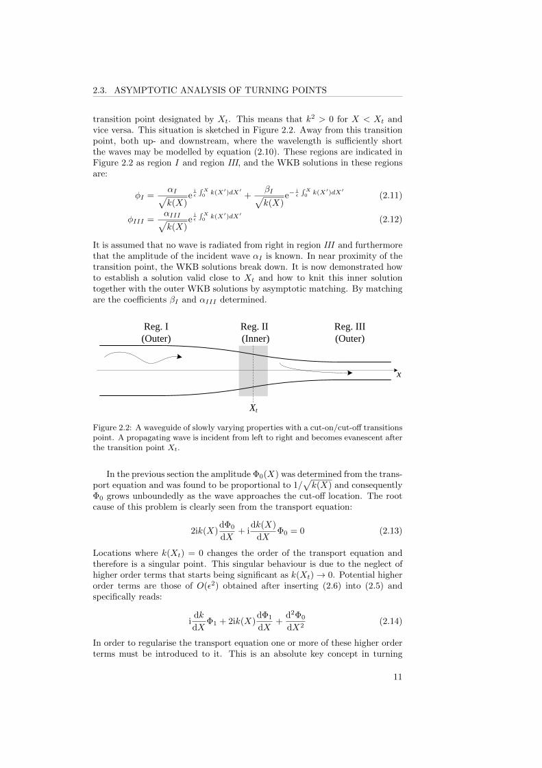
2.3. ASYMPTOTIC ANALYSIS OF TURNING POINTS

transition point designated by Xt. This means that k2 > 0 for X < Xt andvice versa. This situation is sketched in Figure 2.2. Away from this transitionpoint, both up- and downstream, where the wavelength is sufficiently shortthe waves may be modelled by equation (2.10). These regions are indicated inFigure 2.2 as region I and region III, and the WKB solutions in these regionsare:

φI =αI√k(X)

eiε

∫X0k(X′)dX′ +

βI√k(X)

e−iε

∫X0k(X′)dX′ (2.11)

φIII =αIII√k(X)

eiε

∫X0k(X′)dX′ (2.12)

It is assumed that no wave is radiated from right in region III and furthermorethat the amplitude of the incident wave αI is known. In near proximity of thetransition point, the WKB solutions break down. It is now demonstrated howto establish a solution valid close to Xt and how to knit this inner solutiontogether with the outer WKB solutions by asymptotic matching. By matchingare the coefficients βI and αIII determined.

x

Xt

Reg. I (Outer)

Reg. III(Outer)

Reg. II(Inner)

Figure 2.2: A waveguide of slowly varying properties with a cut-on/cut-off transitionspoint. A propagating wave is incident from left to right and becomes evanescent afterthe transition point Xt.

In the previous section the amplitude Φ0(X) was determined from the trans-port equation and was found to be proportional to 1/

√k(X) and consequently

Φ0 grows unboundedly as the wave approaches the cut-off location. The rootcause of this problem is clearly seen from the transport equation:

2ik(X)dΦ0

dX+ i

dk(X)

dXΦ0 = 0 (2.13)

Locations where k(Xt) = 0 changes the order of the transport equation andtherefore is a singular point. This singular behaviour is due to the neglect ofhigher order terms that starts being significant as k(Xt)→ 0. Potential higherorder terms are those of O(ε2) obtained after inserting (2.6) into (2.5) andspecifically reads:

idk

dXΦ1 + 2ik(X)

dΦ1

dX+

d2Φ0

dX2(2.14)

In order to regularise the transport equation one or more of these higher orderterms must be introduced to it. This is an absolute key concept in turning

11

CHAPTER 2. INTRODUCTION TO THE RESEARCH AREA

point studies, and therefore the following steps in the analysis are shown indetail. A scaled version of X is introduced and the scaling is selected such thatsome O(ε2) terms are promoted to be as significant as the original terms in thetransport equation. Before doing so, it is assumed that close to the turningpoint the wavenumber can be expanded by

k2(X) ∼ −c(X −Xt) as X → Xt (2.15)

where c > 0 is a constant. I.e. when X < Xt k(X) is real and the wavepropagates and for X > Xt k(X) is imaginary so the wave is evanescent. Anew scaled coordinate is now introduced:

X = cγεα(X −Xt) (2.16)

The strategy is to select α such that a higher order term from (2.14) is pro-moted to be of same order of magnitude as the O(ε) terms, i.e. the transport

equation. Initially focus is given to the term d2Φ0

dX2 . It will be shown later thatthe remaining terms in (2.14) in fact are negligible. For now this higher orderterm is added to the transport equation as it is:

2ik(X)dΦ0

dX+ i

dk(X)

dXΦ0 + ε

d2Φ0

dX2= 0 (2.17)

Embedding (2.15) and (2.16) in this equation yields:

2ic1/2+γ/2εα/2(−X)1/2 dΦ0

dX− ic1/2+γ/2εα/2(−X)−1/2Φ0 + ε1+2αc2γ

d2Φ0

dX2= 0

(2.18)

The important things to notice are that the first two terms, those originatingfrom (2.13), are still of the same order, specifically O(εα/2). And furthermore,that these balance the latter term, which is O(ε1+2α), provided that α is se-lected as:

α/2 = 1 + 2α ⇔ α = −2/3 (2.19)

It is furthermore noticed that selecting γ = 1/3 makes the c’s cancel throughoutthe equation. What is left now is:

2i(−X)1/2 dΦ0

dX− i

2(−X)1/2Φ0 +

d2Φ0

dX2= 0 (2.20)

I.e. on this new short inner scale X = c1/3(X−Xt)ε2/3 the higher order term ap-

parently is of the same order as the other terms in the transport equation.Remark, that the same rescaling applied to the terms containing Φ1 in (2.14)leaves them at O(ε2/3) which is negligible compared to the terms in (2.20) be-ing O(ε−1/3). This new version of the transport equation is further reduciblewith the help of an integrating factor Φ0(X) = B(X)eg(x) in order to elimi-

nate first order derivatives. By choosing g(X) = −i∫ X

0

√−XdX the equation

conveniently reduces to:

d2B(X)

dX2− XB(X) = 0 (2.21)

12

2.3. ASYMPTOTIC ANALYSIS OF TURNING POINTS

This is Airy’s equation and is one amongst the type of differential equationswith non-constant coefficient to which exact solutions exist. Other examplesof such equations are the Bessel equation and the Parabolic Cylinder equation.The general solution to the Airy equation is a linear combination of the twoAiry function, see for instance [Bender and Orszag, 1978]:

B(X) = c1Ai(X) + c2Bi(X) (2.22)

So, apart from the two constants c1 and c2 the solution in the inner region isnow known. These constants are determined from asymptotic matching to theouter WKB solutions, but before doing so the inner solution is simplified. Theinner solution in terms of φII is:

φII =(c1Ai(X) + c2Bi(X)

)eg(X)e

iε

∫X0k(X′)dX′ (2.23)

It becomes evident that the eikonal part of the solution exp(

iε

∫X0k(X ′)dX ′

)

cancels with the integration factor eg(X) when the latter is expressed in terms ofX rather than X and when the Taylor expansion in (2.15) is employed in placeof k(X). Furthermore, the function Bi(X) grows unbounded for large positivearguments which does not match the evanescent behaviour of the outer solutionand consequently, c2 = 0. What remains is simply:

φII = c1Ai(X) (2.24)

This must now be matched to the outer solution. The procedure for asymptoticmatching is available from textbooks such as [Bender and Orszag, 1978] or[Hinch, 1991], and only a few details is given here. In short, the procedureis to write the inner solution in terms of the outer variable and expand itasymptotically for large arguments. Asymptotic expansions of special functionslike the Airy functions are tabulated in compilations such as [Olver et al., 2010].Expanding the inner solution, equation (2.24) yields:

φII ∼c1

2√π

ε1/6

c1/12(X −Xt)1/4e−23c1/2

ε (X−Xt)3/2

, X →∞ (2.25)

Similarly, by taking the limit X → +Xt (i.e. approaching the turning pointfrom the right) of φIII the following is obtained:

φIII ∼αIIIe

−iπ/4

c1/4(X −Xt)1/4e−23c1/2

ε (X−Xt)3/2

, X → Xt (2.26)

Apparently (2.25) and (2.26) has developed the same functional form and canbe made exactly the same by selecting:

αIIIc−1/4e−iπ/4 = c1

ε1/6

2√πc1/12

(2.27)

In the exact similar fashion may two matching conditions be established bycomparing terms after taking the limits of φII as X → −∞ and φI as X →−Xt, respectively. From these two matching equations and (2.27) the unknown

13

CHAPTER 2. INTRODUCTION TO THE RESEARCH AREA

constants can be determined:

βI = eiπ/2αI (2.28)

αIII = αI (2.29)

c1 =2π1/2eiπ/4

ε1/6c1/6αI (2.30)

This result admits the interpretation that the incident wave is fully reflectedwith a phase shift of π/2. Thus, the energy flux is blocked by the turning point.The example given here is amongst the simplest of its kind, but neverthelessoutlines the approach in a turning point problem. Other kinds of turning pointproblems can be done by assuming another behaviour of k2 around the transi-tion point. This leads to another scaling of the inner region and consequentlyalso another differential equation in the inner region.

Textbooks typically presents a slightly different approach for doing a turn-ing point problem, see for instance [Bender and Orszag, 1978] and [Hinch,1991]. Rather than attempting to promote higher order terms to the transportequation, they simply replace p2(X,ω) in the differential equation (2.5) by itsTaylor expansion around the turning point and from there arrive at Airy’sequation. This approach appears somewhat simpler compared to the expo-sition given above, but this is only the case when tackling Schrodinger typeequations, i.e. where the wavenumber appears directly in the governing differ-ential equation. It is found through the work with more general problems suchas turning points in beams and acoustic ducts that the approach presented inthis section is by far the most instructive.

The second paper included in the thesis, Paper 2, treats the similar, but moreadvanced problem of acoustic waves travelling in a flow duct with a constrictionand determines reflection and transmission coefficients, and a solution which isuniformly valid for all x. The waves undergo a cut-on/cut-off/cut-on transition,i.e. the waves tunnel through the constriction and become propagating againon the other side. In such a case it turns out that the inner region is governedby the Parabolic Cylinder Equation. Furthermore, the duct supports a slowlyvarying flow which also affects the acoustic field and consequently the waveequation to be solved includes convection.

2.3.1 Details on the matching procedure

Performing the asymptotic matching in the above turning point example didnot require a lot of manipulations for the inner and outer solution to have thesame functional form. This not the case in the two turning point problemstudied in Paper 2. In the following it is demonstrated how an intermediatevariable may be employed to identify negligible terms. The problem is specifi-cally that the outer solution in the transmission region close to the rightmostturning point has a phase which is proportional to:

X

2

√X2 − b− b

2ln

(X −

√X2 − b√b

)(2.31)

14

2.4. PERIODICITY EFFECTS

but the corresponding terms in the inner solution for large positive argumentsis:

X2

2− b

2ln

(2X√b

)(2.32)

and therefore there is no apparent match between the two. The inner coor-dinate for the problem is denoted z and defined by z = G X

ε1/2 where G is

some constant. An intermediate variable is now introduced Y = Xεβ

where0 < β < 1/2. I.e. Y lies between X and z and therefore helps estimating ifany terms in (2.31) may be neglected. The outer solution with X replaced byY and b = εb, see Paper 2 for details, is therefore:

Y 2ε2β

2

√1− ε1−2β

b

Y 2− εb

2ln

Y ε

β + Y εβ√

1− ε1−2β bY 2√

εb

(2.33)

By the binomial expansion this becomes

Y 2ε2β

2− ε b

4− εb

2ln

(2Y εβ − ε1−β b

2Y√εb

)(2.34)

Since β is strictly smaller 1/2 then we notice that 2Y εβ >> ε1−β b2Y as ε→ 0.

Thus, (2.31) becomes:

X2

2− b

4− b

2ln

(2X√b

)(2.35)

which has the same X dependence as (2.32) and a matching condition cantherefore be identified. The term b/4 corresponds to a constant phase shift.

As a last comment it is mentioned that to generate the results presented inPaper 2 has it been necessary to implement the Parabolic Cylinder Functionwhich have a few different definitions U(a, z), V (a, z), Dν(z) and W (a, x). Thefunction W (a, x) is the one needed. In the preferred software (Mathematica)the function Dν(z) exists and by combining formulae from [Olver et al., 2010,ch. 12] a definition of W (a, x) can be implemented.

2.4 Periodicity effects

The application of the theory of periodic waveguides employed is so limitedthat only very little introduction to this is needed. Consequently, is only avery short exposition of elementary Floquets theory given and focus is thenturned to various other techniques employed in the research.

The theory of wave propagation in periodic structures typically concerns anal-ysis of a structure composed of a number of segments of various structuralmembers forming a unit cell. A number of consecutive unit cells form a pe-riodic structure. If the individual segments are simple enough exact solutionsare available to describe the wave motion in these. This is advantageous sincea unit cell can be modelled by matching the individual segments at the internal

15

CHAPTER 2. INTRODUCTION TO THE RESEARCH AREA

interfaces. The waveguide properties of the periodic structure are then obtain-able by Floquets theorem which shall be introduced briefly in the following.

In short the Floquet theorem states that the solution to an ordinary differ-ential equation with 2π periodic coefficients is, [Bender and Orszag, 1978]:

y(t) = λy(t+ 2π) (2.36)

where λ is a propagation constant. It is the quantity λ that is of interest sinceit relates directly to wave attenuation. In the practical usage of the Floquettheorem waveguides of arbitrary period, say L, are typically studied.

xn xn+1 xn+2 xn+3xn-1 x

un un+1un-1

L

Figure 2.3: A periodic rod consisting of a number of unit cells of length L.

The work on periodicity effects in this thesis is applied to simple axialwaves in a Bernoulli-Euler rod consisting of unit cells with segments of differentproperties. An illustration is provided in Figure 2.3. The result of applyingthe periodicity conditions is an eigenvalue problem leading to a characteristicequation which links the propagation constant λ to the frequency ω.

The simplicity of the model facilitates understanding the underlying mech-anisms behind stop bands. Consequently, have much effort been given to es-tablish relations between the propagation constant λ, waveguide parametersand frequency. It turns out that the use of non-dimensional scaling condensesthe waveguide parameters to just two principal parameters, both having a clearphysical meaning. These are the ratio of impedances and the ratio of propaga-tion times of the two segments in a unit cell.

Parts of the study have been conducted as asymptotic analysis where ex-pressions for stop band borders are derived by perturbing the impedance mis-matches between the segments in the unit cell. This relies on the methodologyof finding solution to algebraic equation containing a small parameter. A se-lection of illustrative examples on such problems are provided in [Hinch, 1991]and in [Bender and Orszag, 1978].

An important aspect of the dynamics of periodic structures is the link be-tween the stop band borders and eigenfrequencies of the symmetric unit cell.This fact is discussed in [Mead, 1970] and it is recognised that the eigenfre-quencies of the symmetric unit cell with borders fully fixed or free are locatedon the borders of the stop bands. This correspondence has been observedand commented on by other authors, but it does not appear to be very wellunderstood. The work on periodicity effects applied to axial waves attemptsto utilise this observation in the search for simple formulae useful to predictthe band gap structure. To study this and other coherencies between reso-nances and periodicity effects have the Phase-closure Principle been utilisedand found well suited. In the following is a simple exposition of the phaseclosure principle given. A more complete demonstration is provided by Mead[1994], who demonstrates how to derive eigenfrequencies of Bernoulli-Euler

16

2.4. PERIODICITY EFFECTS

kxie

kx-ie

RieLie

L

Figure 2.4: A finite length rod with indication of right and left going waves andreflections at the boundaries.

beams with various boundary conditions. By the phase closure principle theresonance condition is formulated via the phase change a wave experiences af-ter completing a circuit in a finite length rod like the one shown in Figure 2.4.For simplicity the rod is assumed to support axial waves only. The completephase change is found by summation of the phase change caused by traversingforth and back in the rod, which amounts to 2kL, and the phase shifts fromthe reflections at the right and left boundaries, ϕR and ϕL, respectively. Whenthe total phase change adds up to an integral multiple of 2π resonance occurs.Physically this corresponds to the wave returns back perfectly in phase withitself. Thus, we may state:

2kL+ ϕR + ϕL = n2π (2.37)

By designating the plane stress wave speed as c0 and assuming free-free bound-aries, i.e. ϕR = ϕ = L = 0, the above equation becomes:

2ω

c0L = n2π ⇒ ω =

nπc0L

with n = 0, 1, 2, 3, . . . (2.38)

This is also the expression given in [Rao, 2004]. In case either one or bothof the boundaries were fixed ϕL and/or ϕR would be −π, and the eigenfre-quencies would change accordingly. The phase closure principle is expedientin the case where the wave motion and the reflection at the boundaries aregiven by relatively simple expressions. I.e. where the frequency does not ap-pear in the argument of, say, a trigonometric function in the expression for thephase change at the boundaries. It is demonstrated in [Mead, 1994] how theneglect of evanescent waves in a fully fixed Bernoulli-Euler beam leads to avery simple, yet very accurate, explicit formula for natural frequencies. Mead[1994] also demonstrates that with account of evanescent waves the well-knowntranscendental equation for eigenfrequencies quoted in standard textbooks areobtained by the phase closure principle.

Paper 3 is initiated from considerations about the fundamental cancellationmechanism behind stop bands, and a wish to establish some simple relationsbetween waveguide properties and locations of stop and pass bands. It is forthese reasons the very simple Bernoulli-Euler model for axial waves has beenselected as the focal point of the paper. In the pursuit of these simple re-lations that perturbative analysis and the phase closure principle have beenused. The results from here lead to the main conclusions in the paper. The pa-per lastly presents an analysis of steady-state and transients of a finite length

17

CHAPTER 2. INTRODUCTION TO THE RESEARCH AREA

periodic rod. It is demonstrated how energy accumulates develops depend-ing on whether excitation is done in a stop band, in a pass band, or at aneigenfrequency.

18

Chapter 3

Summary of results

This chapter gives a brief discussion of the main findings from each of thethree journal papers that are part of the thesis. To each paper are reflectionsof potential extensions discussed and important limitations of the work areprovided. This leads to reasoning on why the topic of the subsequent paperhas been selected.

3.1 Paper 1

In this paper WKB solutions are derived in a systematic manner for a hierar-chy of beam models of slowly varying diameter. The models are the Rayleighbeam, the Timoshenko beam, and a planar curved Timoshenko beam, governedby one, two, and three differential equations, respectively. The numerical per-formance of the solutions is tested by comparison to reference solutions and avalidity criterion is presented.

It is found that apart from the location dependence of parameters thewavenumber is the same as in the unperturbed waveguide, and therefore thiswill typically be known in advance. This is a major advantage of the methodsince only little derivation is needed. Another important confirmation in thepaper is that the variation of wavenumber and amplitude corresponds to en-ergy conservation. I.e. a wave propagates with constant energy even thoughthe wavenumber and amplitude varies.

From the approach demonstrated in the paper it is quite obvious how toderive WKB solutions for other beam structures such as beams of constant crosssection, but with for instance slowly varying planar or spatial curvature. Suchresults are potentially of direct practical relevance in modelling of vibrations ofsuspension systems. The paper also demonstrates that the WKB method doesnot immediately lead to any wave attenuation. It merely gives a modulation ofthe wave. This is mainly the reason why the concepts of turning point analysisand tunnelling effects have been included as topics to be studied.

3.2 Paper 2

In this paper tunnelling of acoustic waves in a flow duct with a constriction isanalysed. By asymptotic matching between outer WKB type solutions validaway from the constriction and an inner solution valid in the near vicinity of

19

CHAPTER 3. SUMMARY OF RESULTS

the constriction expressions for reflections and transmissions coefficients aredetermined. A uniformly valid solution is furthermore derived and its corre-spondence to the composite solution is demonstrated.

The results are potentially important to engineers designing aero-craft en-gines since the results presented further enhance the opportunity to use multi-ple scales methods to determine the sound field through the duct. The responseto any sound source can be determined by modal expansion and with the re-sults presented in this paper the effect of modes tunnelling in the engine ductcan now be accounted for.

The technique readily suggests how to tackle turning point problems inelasticity. In line with the models treated in Paper 1 could this be cut-off offlexural waves in varying Bernoulli-Euler beams resting on an elastic founda-tion, shear wave cut-off in a varying Timoshenko beam, or turning points inbeams of varying curvature. It is generally found that the technique behindturning point studies is advanced, but the results are general and therefore canbe directly applied to various acoustic duct problems and moreover do theyhave a clear physical meaning. The methodology is, however, still consideredas having limited potential as regards gaining control over wave propagation,since wave reflection or attenuation relies on the presence of cut-on/cut-offtransition points. Thus, all modes of higher frequencies than that of the cut-on/cut-off mode will propagate past the transition point. Additional turningpoints should therefore be introduced to the waveguide to prevent these higherfrequency modes from propagating. For these reasons, attention is turned toperiodicity effects in the third paper.

3.3 Paper 3

In this paper various studies on axial waves in a periodic Bernoulli-Euler rodhave been conducted. The focus is to understand the cancellation mechanismbehind stop bands. This has been done by perturbative analysis of the eigen-value problem from the Floquet analysis. The principle of phase closure isfurthermore adopted and relations between resonance criteria and stop bandlocations are identified.

The results presented provide an easily understood overview of where stopbands are located depending on waveguide parameters, and consequently howparameters should be chosen to have stop bands in desired frequency ranges.The explanation of the stop band pattern and the formulae describing stop andpass band locations are considered so simple that these can be used actively in adesign process. Despite these motivating findings should it be remembered thatthe similar knowledge for dispersive flexural waves is not available and thereforethe results are likely insufficient for more general excitation condition. As alast comment should it also be noticed that if steel is selected as the materialand the individual segment length are at maximum the order of a few metersthen the first stop band is found at least at the kHz-level. In many practicalapplications this would indeed be a very high frequency, and there would likelybe an interest to have stop bands at much lower frequencies.

20

3.4. CONTRIBUTION AND IMPACT

3.4 Contribution and impact

The use of the WKB method to study curved Timoshenko beams of varyingdiameters and identifying the combination of validity criterion for multi-modalproblems are definite contributions. To the authors knowledge no studies arereported treating such complex elastic beams which also contains a presenta-tion of numerical performance. The generalised criterion for validity presentedin the paper where both the small parameter ε and amount of variation ofthe waveguide also appears to be new. This leads to the key finding that anoverlap of validity ranges exists between the plane cross section models and theWKB approximation. Consequently, it is confirmed that the WKB method isavailable to the analyst.

The research on tunnelling effects of acoustic waves propagating in flow ductscontributes to the pool of solutions available to predict noise transmission in forinstance aero-craft engines. Thus, the results will potentially help engine de-signers to apply multiple scales methods to estimate the noise pollution, detectresonance from reflected waves, etc. The result may furthermore serve as animportant benchmark solution to computational aero-acoustic codes. Finally,does the numerical result serve as an illustrative demonstration of tunnelling.

In paper 3 are explicit expressions given that very accurately describe thelocation of stop band borders at small and large impedance mismatches. To theauthor’s knowledge this is the first time such a result have been presented forperiodic waveguides consisting of continuous structural segments. The model islikely to primitive for the results to be practically applicable, but the method-ology and the nature of the results may impact how periodic structures areanalysed. In particular, similar results obtained for more complex waveguideswill contribute to the ability to easily tailor the dynamic properties of a con-struction.

21

Chapter 4

Concluding remarks

The objectives of this work has been to investigate methods to predict wavepropagation in various kinds of non-uniform waveguides, to gain insight in theunderlying mechanism behind wave attenuation, and to identify simple rela-tions between wave propagation and waveguide parameters. This has beendone with a bias to use asymptotic and perturbative methods to retrieve dom-inant terms in solutions to wave equations. The work has been carried outwithin the framework of linear dynamics and specifically have acoustic flowducts, non-uniform beams and periodic rods been considered.

A methodology to study waves in slowly varying beams is investigated witha subsequent test of numerical accuracy, and a criterion for validity is estab-lished. The special case of acoustic waves diminishing by tunnelling throughnarrow regions of evanescent wave motion in flow ducts is studied and reflectionand transmission coefficients depending on tunnelling distance are derived. Fi-nally, the cancellation mechanism behind stop bands is studied for axial wavesin a periodic rod. It is discovered how resonance criteria for a unit cell andthe individual segments correlate to the location of stop and pass bands. It isdemonstrated how these locations can be found simply by the application ofthe phase closure principle.

Consequently, the overall objective of increasing the understanding of the effectof non-uniformity on wave propagation in slender waveguides is fulfilled.

4.1 Future works

An obvious extension on the topic of slowly varying beams would be to derivesolutions similar to those presented in Paper 1, but for planar or spatial cur-vature in order to predict vibrations in for instance suspension systems madefrom curved beams of perturbed helical shape. In order to account for inter-nal reflection of waves in such waveguides turning point analysis should beconducted. This will provide some, but limited options to control the wavepropagation.

The analysis provided in Paper 2 is an extension of the numerous studies of theone turning point problems handled in papers on flow duct acoustics publishedover the last few decades. These papers have advanced on several other fronts

23

CHAPTER 4. CONCLUDING REMARKS

compared to the setup up in Paper 2. For instance, the following challengingfeatures are accounted for: arbitrary cross sectional shape of duct, transitionfrom annular to hollow shape, and inclusion of a significant mean swirl. Theseextensions are as relevant to the two turning point problem as they are to theone turning point problem.

The concept behind turning point analysis presented in 2.3 is just as wellapplicable to varying beams and rods. A natural problem to study could bethat of turning points of flexural waves in a Bernoulli-Euler rod resting on aWinkler foundation.

The work presented in Paper 3 suggests many aspects of future work. An im-mediate extension would be to carry out the similar analysis for a unit cell ofthree or four different segments. This will likely lead to a more complex stopband pattern compared to that of Paper 3. The subsequent analysis of stopband borders, stop band pattern, and application of the phase closure principlewill therefore be more challenging. It may, however, provide an option to pushthe first stop bands towards lower frequencies. A central assumption in Paper3 is the sole existence of non-dispersive waves and extending the analysis toincluded dispersive waves, such as flexural waves, is therefore highly relevant.In line with the suggestions for extensions made to Paper 1, it is certainly ofinterest to extend the results from Paper 3 to unit cells with curved segmentsthat conveys flexural, axial and torsional waves. The accessibility of resultssimilar to those presented in Paper 3 valid to such complicated periodic beamswill likely provide a very powerful and relative easily applied tool to design ofmechanical filters.

An interesting aspect of analysing periodic beam structures partly consistingof segments of gradually varying properties is now suggested. By the quiteefficient approach to predict wave propagation in gradually varying beams pre-sented in Paper 1 and with the knowledge of internal reflection in line withthe results presented in Paper 2 these gradually varying segments can be anal-ysed with relative ease. In particular, the phase changes the various wavesexperience when travelling in a segment are obtainable from the slowly varyingdispersion relation. In Paper 3 it is shown that this phase change is essential inthe prediction of stop and pass band. If the analysis is extended successfully tostudy waveguides of such complexity, it will likely serve as a very powerful al-ternative to computational methods such as the FE method with an associatednumerical optimisation routine.

24

References

C. M. Bender and S. A. Orszag. Advanced Mathematical Methods for Scientists andEngineers. Springer, 1978. ISBN 0-387-98931-5.

E. Brambley and N. Peake. Sound transmission in strongly curved slowly varyingcylindrical ducts with flow. Journal of Fluid Mechanics, 596:387–412, 2008.

L. Brillouin. Wave propagation in periodic structures. Dover Publications, 1946.

A. J. Cooper and N. Peake. Propagation of unsteady distubances in slowly varyingduct with mean swirling flow. Journal of Fluid Mechanics, 445:207–234, 2001.

A. J. Cooper and N. Peake. The stability of a slowly diverging swirling jet. Journalof Fluid Mechanics, 473:389–411, 2002.

R. D. Firouz-Adabi, H. Haddadpour, and A. B. Novinzadeh. An asymptotic solu-tion to transverse free vibrations of variable-section beams. Journal of Sound andVibration, 304:530–540, 2007.

N. Froman and P. O. Froman. Physical Problems Solved by the Phase-Integral Method.Cambridge University Press, 2004. ISBN 0-511-02995-0.

J. Heading. An Introduction to Phase-Integral Methods. Dover Publications, Inc,2013. ISBN 0 486 49742 9.

E .J. Hinch. Perturbation Methods. Cambridge University Press, 1991. ISBN 0 52137310 7.

J. S. Jensen. Phononic band gaps and vibrations in one- and two-dimensional mass-spring structures. Journal of Sound and Vibration, 266:1053–1078, 2003. doi:10.1016/S0022-460X(02)01629-2.

J. S. Jensen and N. L. Pedersen. On maximal eigenfrequency separation in two-material structures: the 1d and 2d scalar cases. Journal of Sound and Vibration,289:967–986, 2006.

V. Krylov and S. V. Sorokin. Dynamics of elastic beams with controlled distributedstiffness parameters. Smart. Mater, Struct, 6:573–582, 1997.

B. M. Kumar and R. I. Sujith. Exact solutions for the longitudinal vibration ofnon-uniform rods. Journal of Sound and Vibrations, 207:721–729, 1997.

S. Lenci, F. Clementi, and C.E.N. Mazzilli. Simple formulas for the natural frequenciesof non-uniform calbes and beams. International Journal of Mechanical Sciences,77:155–163, 2013.

D. J. Mead. Free wave propagation in periodically supported, infinite beams. Journalof Sound and Vibration, 11:181–197, 1970. doi: 10.1016/S0022-460X(70)80062-1.

25

REFERENCES

D. J. Mead. Waves and modes in finite beams: Application of the phase-closureprinciple. Journal of Sound and Vibration, 171:695–702, 1994. doi: 10.1006/jsvi.1994.1150.

D. J. Mead. Wave propagation in continuous periodic structures: Research contribu-tions from southampton, 1964-1995. Journal of Sound and Vibration, 190:495–524,1996. doi: 10.1006/jsvi.1996.0076.

N. Olhoff, B. Nui, and G. Cheng. Optimum design of band-gap beam structures.International Journal of Solids and Structures, 49:3158–3169, 2012. doi: 10.1016/j.ijsolstr.2012.06.014.

F. W. J. Olver, D. W. Lozier, R. F. Boisvert, and C. W. Clark, editors. NISTHandbook of Mathematical Functions. Cambridge University Press, New York,NY, 2010.

N. C. Ovenden. A uniformly valid multiple scales solution for cut-on cut-off transitionof sound in flow ducts. Journal of Sound and Vibration, 286:403–416, 2005.

A. D. Pierce. Physical interpretation of the wkb or eikonal approximation for wavesand vibrations in inhomogeneous beams and plates. Acoustical Society of America,pages 275–284, 1969.

S. S. Rao. Mechanical Vibrations. PEARSON, Prentice Hall, 2004. ISBN 0-13-120768-7.

S. W. Rienstra. Sound transmission in slowly varying circular and annular lined ductswith flow. Journal of Fluid Mechanics, 380:279–296, 1999.

S. W. Rienstra. Sound propagation in slowly varying lined flow ducts of arbitrarycross-section. Journal of Fluid Mechanics, 495:157–173, 2003.

G. Rosenfeld and J. B. Keller. Wave propagation in nonuniform elastic rods. Acous-tical Society of America, pages 1094–1096, 1975.

S.Abrate. Vibration of non-uniform rods and beams. Journal of Sound and Vibrations,184:703–716, 1995.

A. Søe-Knudsen. Design of stop-band filter by use of curved pipe segments andshape optimization. Struct Multidisc Optim, 44:863–874, 2011. doi: 10.1007/s00158-011-0691-2.

26

Paper 1

Nielsen R.B, Sorokin S.V. (2014): ”The WKB approximation for analysis ofwave propagation in curved rods of slowly varying diameter”, Proceedings ofthe Royal Society A 470

27

PAPER 1

28

rspa.royalsocietypublishing.org

ResearchCite this article: Nielsen R, Sorokin S. 2014The WKB approximation for analysis of wavepropagation in curved rods of slowly varyingdiameter. Proc. R. Soc. A 470: 20130718.http://dx.doi.org/10.1098/rspa.2013.0718

Received: 29 October 2013Accepted: 25 March 2014

Subject Areas:mechanical engineering, applied mathematics

Keywords:WKB approximation, asymptotic analysis,wave propagation, non-uniform rods

Author for correspondence:Rasmus Nielsene-mail: rn@m-tech.aau.dk

The WKB approximation foranalysis of wave propagationin curved rods of slowlyvarying diameterRasmus Nielsen and Sergey Sorokin

Department of Mechanical and Manufacturing Engineering,Aalborg University, Fibigerstraede 16, 9220 Aalborg, Denmark

The Wentzel–Kramers–Brillouin (WKB) approxim-ation is applied for asymptotic analysis of time-harmonic dynamics of corrugated elastic rods. Ahierarchy of three models, namely, the Rayleigh andTimoshenko models of a straight beam and theTimoshenko model of a curved rod is considered.In the latter two cases, the WKB approximationis applied for solving systems of two and threelinear differential equations with varying coefficients,whereas the former case is concerned with a singleequation of the same type. For each model, explicitformulations of wavenumbers and amplitudes aregiven. The equivalence between the formal derivationof the amplitude and the conservation of energy flux isdemonstrated. A criterion of the validity range of theWKB approximation is proposed and its applicabilityis proved by inspection of eigenfrequencies of beamsof finite length with clamped–clamped and clamped-free boundary conditions. It is shown that there isan appreciable overlap between the validity rangesof the Timoshenko beam/rod models and the WKBapproximation.

1. IntroductionThe Wentzel–Kramers–Brillouin (WKB) approximationis a well-established and recognized tool in theoreticalphysics in general, and in quantum mechanics inparticular. Its application for solving the Schrödingerequation provides simple-structured solutions thatdescribe the motion of particles and phenomena such astunnelling. Examples can be readily found in classicalcompilations and textbooks such as Fröman & Fröman [1]or Bender & Orszag [2]. The fundamental feature of theWKB method is its ability to approximate the solutions of

2014 The Author(s) Published by the Royal Society. All rights reserved.

on August 13, 2014rspa.royalsocietypublishing.orgDownloaded from

2

rspa.royalsocietypublishing.orgProc.R.Soc.A470:20130718

...................................................

linear differential equations with varying coefficients. This unique characteristic of the methodimmediately suggests its suitability for describing wave motion in inhomogeneous media andconsequently the method has found its way to the field of acoustics. For problems of wavepropagation in non-uniform acoustic ducts the method has been applied by for instance Rienstra[3], Cooper & Peake [4] and Brambley & Peake [5]. The method has also been applied inelastodynamics and, more specifically, for analysis of wave motion of planar curved elastic stripsby Scott & Woodhouse [6], guided waves in a circular elastic annulus by Gridin et al. [7], andstraight non-uniform rods in plane stress by Rosenfeld & Keller [8].

Another class of problems in elasticity where the WKB method is applicable, but, to the bestof the authors knowledge has not yet been used profoundly, is the wave propagation in non-uniform rods in the framework of the classical ‘plane cross-sectional’ model. The pioneeringwork along these lines has been done by Pierce [9], who used the WKB method to determinethe wavenumbers in straight inhomogeneous Bernoulli–Euler and Timoshenko beams. However,the amplitude variation was determined from the energy conservation condition, rather thanby means of the formal WKB approximation. An expression for the eigenfrequencies of acantilevered Bernoulli–Euler beam is presented in the paper, with no numerical results beingreported. In a paper by Langley [10], the propagation of flexural waves in a straight Bernoulli–Euler beam was studied by deriving a short-wave perturbation solution similar to a WKBsolution. The short-wave perturbation solution found in Langley [10] was derived after recastingthe governing equation to a first-order matrix vector system and transform this to ‘wavecoordinates’ based on the eigenvectors and eigenvalues of the system. More specifically the caseanalysed was the reflection and transmission coefficients for a non-uniform pre-compressed beamresting on an elastic foundation with non-uniform properties.

A relatively low interest in the WKB approximations in the classical rod theories can beexplained by an obvious contradiction between the limitations of the two. Namely, the WKBapproximation is, in essence, a short-wave or high-frequency method, whereas the classical rodtheories are formulated for long-wave or low-frequency wave motion. More specifically, theTimoshenko beam model may be regarded as accurate up to and slightly above the shear wavecut-on [11], whereas the validity range for the Bernoulli–Euler beam model is much narrower.This naturally raises the question on whether there is an appreciable overlap of frequencies,where both the plane cross-sectional hypothesis and the WKB approximation are valid. Toanswer this question, results determined by the WKB method should be compared with resultsdetermined by a substantially different method, for example, by numerical solutions. In theabove-mentioned references on rods, such a comparison has not been done and one of the goalsof this paper is to accomplish this. This is done by comparing eigenfrequencies determinedby the WKB method and numerical methods for various rods when specialized to differentboundary conditions. Determining eigenfrequencies of non-uniform beams as done in this paperis, however, not the main motivation of using the WKB method, but rather eigenfrequencies areregarded as a convenient measure to assess the accuracy of the WKB method when applied toplane cross-sectional problems.

Analysis of elastic waves in non-uniform beams by the WKB approximation is useful inmany practical aspects. Asymptotic analysis is, in general, known as a powerful tool to revealthe underlying physics of complicated problems and to provide some approximate yet simpleand useful relationships between the parameters of a given problem and its solution. Theseinsights can greatly facilitate the engineer during the design process of, say, a suspension systemcomposed of non-uniform beams. The important information on wave propagation, cut-on/cut-off frequencies, etc., of a non-uniform waveguide, available from the WKB method is quite uniqueas no standard numerical method provides that.

The classical application of the WKB approximation in quantum mechanics (or in linearacoustics) is concerned with solving a single partial differential equation of the second orderwith varying coefficients. In elastodynamics, the approximation is applied to solve a system oftwo differential equations, which are of the second order each. The motion of curved rods inthe framework of Timoshenko formulation are generally governed by six coupled differential

on August 13, 2014rspa.royalsocietypublishing.orgDownloaded from

3

rspa.royalsocietypublishing.orgProc.R.Soc.A470:20130718

...................................................

R*

s*

j,ui,w

d−*

k,b

Figure 1. Curved corrugated rod.

equations with varying coefficients and therefore the WKB solution of three coupled equations,representing a planar curved corrugated Timoshenko rod, reported in this paper contains aspectsof novelty in its own right.

The study presented in this paper is devoted to demonstrate how the WKB method isgeneralized to, in a formal manner, solve systems of differential equations with slowly varyingcoefficients and to demonstrate that there is an appreciable overlap between the high-frequencyWKB method and the low-frequency theory of rods, which employs the plane cross-sectionalhypothesis. The application of the WKB approximation will be exemplified on the followingnon-uniform elastic members: (i) straight Rayleigh rod, (ii) straight Timoshenko rod and (iii) curvedTimoshenko rod. This choice of increasingly advanced models will accomplish the demonstrationof how simple and systematic the WKB approximation in fact is. In §4, the accuracy of the WKBsolutions when applied to elasticity problems based on the plane cross-sectional hypothesis isgauged. This is done by the aforementioned comparison of eigenfrequencies.

2. Models of non-uniform beamsConsider a rod with a circular cross section with a varying diameter and define the axial lengthscale of inhomogeneity as l∗ (∗ denotes dimensional quantities), i.e. this is the length over whichthe diameter changes significantly. More specifically, the diameter may be defined as

d∗(s∗) = d∗ + d′∗ sin(

s∗

l∗

), (2.1)

where d∗ is the mean diameter, as indicated in figure 1, d′∗ is the change in diameter and s∗ isthe axial coordinate. By scaling lengths using d∗, the non-dimensional diameter can be stated asd(s) = 1 + r sin(εs), where r = d′∗/d∗ and ε = d∗/l∗. The requirement for slow variation of the crosssection is then ε 1. Thus, the diameter is dependent on a slow coordinate d∗(εs), and likewiseare the area and moment of inertia: A∗(εs) = (π/4)d∗2(εs), I∗(εs) = (π/64)d∗4(εs). This is the typicalway of stating the requirement of slow variation of a waveguide even though nothing, at thisstage, is said about the wavelength. It will be shown later on that stating ε 1 is not by itselfsufficient to ensure accuracy of the WKB approximation.

The key assumption in classical rod theories is the assumption that a cross section remainsplane in the course of deformation. The simplest of these models is the classical Bernoulli–Euler model, in which the cross section is additionally assumed to remain perpendicular to themiddle axis during deformation [12]. This has the immediate consequence that the deformationof the beam is completely given by the lateral deflection u∗(s∗, t∗) of the centreline. Owingto this assumption, the elastic energy stems only from the deflection caused by the bendingmoment, which is given by Q∗(s∗, t∗) = −E∗I∗(s)(∂2u∗(s∗, t∗)/∂s∗2), where E∗ is Young’s modulus,thus the elastic energy density is v∗ = 1

2 Q∗(s∗, t∗)(−∂2u∗(s∗, t∗)/∂s∗2). So the elastic energy of aBernoulli–Euler beam is

V∗ = 12

∫L∗

0E∗I∗(s∗)

(∂2u∗(s∗, t∗)

∂s∗2

)2

ds∗, (2.2)

on August 13, 2014rspa.royalsocietypublishing.orgDownloaded from

4

rspa.royalsocietypublishing.orgProc.R.Soc.A470:20130718

...................................................

where L∗ is the length of the beam. The kinetic energy of a beam under deformation is

T∗ = 12

∫L∗

0

⎡⎣ρ∗A∗(s∗)

(∂u∗(s∗, t∗)

∂t∗

)2+ ρ∗I∗(s∗)

(∂2u∗(s∗, t∗)

∂s∗∂t∗

)2⎤⎦ds∗, (2.3)

where ρ∗ is the mass density. The first term in (2.3) is the conventional Bernoulli–Euler inertiaterm and the second term is the rotary inertia correction term introduced by Rayleigh [13].For that reason, this model will henceforth be referred to as the Rayleigh beam model. Thegoverning equation of such a beam can be found by setting up the action integral and usingHamilton’s principle

0 = δ

∫ t∗2

t∗1(T∗ − V∗) dt∗ =

∫ t∗2

t∗1

∫L∗

0

[ρ∗A∗(s∗)

∂u∗(s∗, t∗)∂t∗

δ∂u∗(s∗, t∗)

∂t∗

+ ρ∗I∗(s∗)∂2u∗(s∗, t∗)

∂s∗∂t∗δ∂2u∗(s∗, t∗)

∂s∗∂t∗

− E∗I∗(s∗)∂2u∗(s∗, t∗)

∂s∗2 δ∂2u∗(s∗, t∗)

∂s∗2

]ds∗ dt∗. (2.4)

Integrating by parts the first term once, the second and the third term twice, and omitting thecorresponding boundary terms one arrives at the following governing equation:

0 = ρ∗A∗(s∗)∂2u∗(s∗, t∗)

∂t∗2 − ρ∗ ∂

∂s∗

(I∗(s∗)

∂3u∗(s∗, t∗)∂s∗∂t∗2

)

+ E∗ ∂2

∂s∗2

(I∗(s∗)

∂2u∗(s∗, t∗)∂s∗2

). (2.5)

Let the temporal dependency throughout this paper be given by e−iω∗t∗ and then scale lengths byd∗ and frequency by

√E∗/ρ∗/d∗. Applying this yields the following ordinary differential equation:

0 = −ω2A(s)u(s) + ω2 dds

(I(s)

du(s)ds

)+ d2

ds2

(I (s)

d2u(s)ds2

). (2.6)

Unlike the Rayleigh beam model, the Timoshenko beam model does not assume the cross sectionto remain perpendicular to the centreline during deformation and therefore introduces a newvariable that measures the cross-sectional rotation β(s∗, t∗). Thus, the shear force in a Timoshenkobeam cannot be determined only from the deflection of the centreline, but rather by the differencebetween the slope of the centreline and the rotation of a cross section

P∗ = λG∗A∗(s∗)(

∂u∗(s∗, t∗)∂s∗ − β(s∗, t∗)

), (2.7)

where λ is the shear correction factor, which is dimensionless, and G∗ is the shear modulus, whichis rewritten by G∗ = E∗/(2(1 + ν)) where ν is Poisson’s ratio which is also dimensionless. Theinternal moment is given by

Q∗ = −E∗I∗(s∗)∂β(s∗, t∗)

∂s∗ . (2.8)

The elastic and kinetic energy is then

V∗ = 12

∫L∗

0

[E∗I∗(s∗)

(∂β(s∗, t∗)

∂s∗

)2+ κG∗A∗

(∂u∗(s∗, t∗)

∂s∗ − β(s∗, t∗))2

]ds∗ (2.9)

and

T∗ = 12

∫L∗

0

[ρ∗A∗(s∗)

(∂u∗(s∗, t∗)

∂t∗

)2+ ρ∗I∗(s∗)

(∂β(s∗, t∗)

∂t∗

)2]

ds∗. (2.10)

The equations governing the motion of a Timoshenko beam is then found by setting up the actionintegral and apply Hamilton’s principle by performing variations with respect to u∗(s∗, t∗) and

on August 13, 2014rspa.royalsocietypublishing.orgDownloaded from

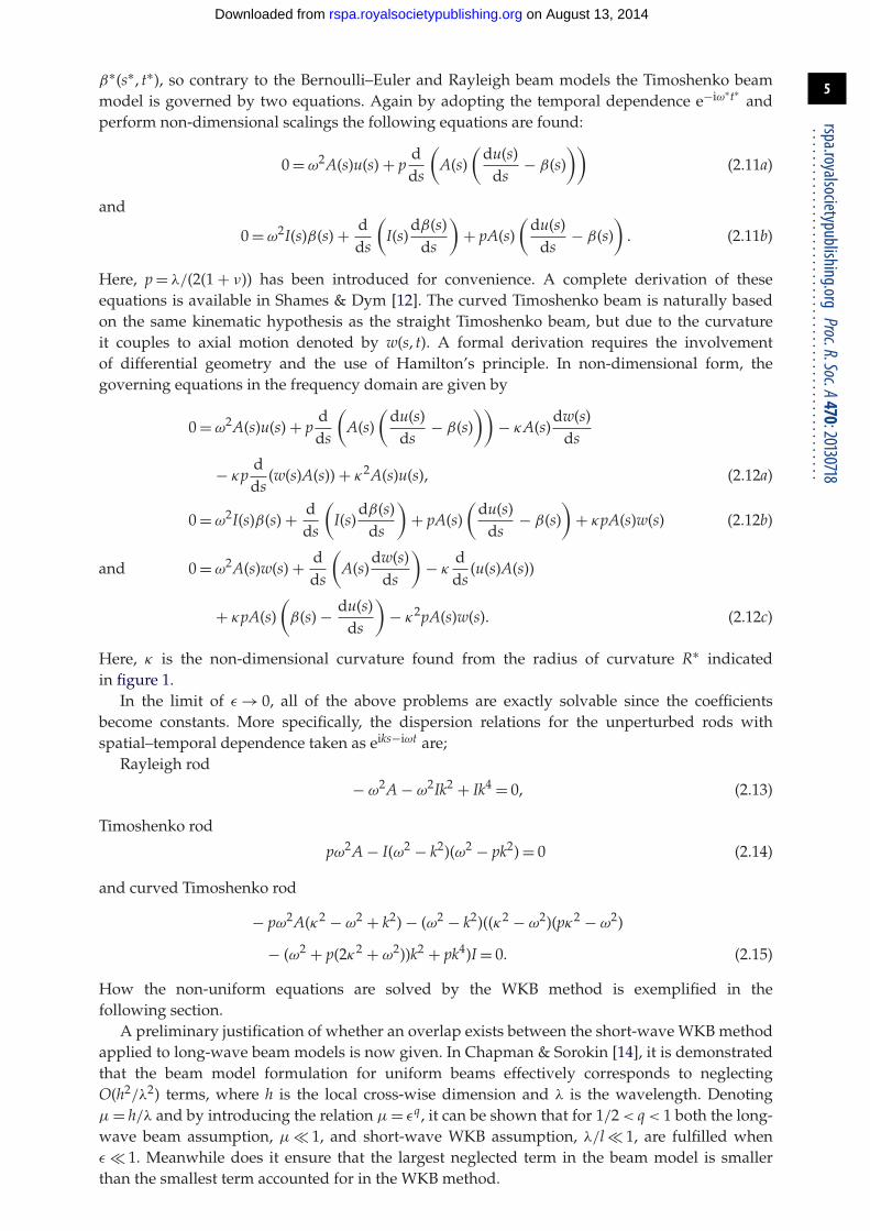
5

rspa.royalsocietypublishing.orgProc.R.Soc.A470:20130718

...................................................

β∗(s∗, t∗), so contrary to the Bernoulli–Euler and Rayleigh beam models the Timoshenko beammodel is governed by two equations. Again by adopting the temporal dependence e−iω∗t∗ andperform non-dimensional scalings the following equations are found:

0 = ω2A(s)u(s) + pdds

(A(s)

(du(s)

ds− β(s)

))(2.11a)

and

0 = ω2I(s)β(s) + dds

(I(s)

dβ(s)ds

)+ pA(s)

(du(s)

ds− β(s)

). (2.11b)

Here, p = λ/(2(1 + ν)) has been introduced for convenience. A complete derivation of theseequations is available in Shames & Dym [12]. The curved Timoshenko beam is naturally basedon the same kinematic hypothesis as the straight Timoshenko beam, but due to the curvatureit couples to axial motion denoted by w(s, t). A formal derivation requires the involvementof differential geometry and the use of Hamilton’s principle. In non-dimensional form, thegoverning equations in the frequency domain are given by

0 = ω2A(s)u(s) + pdds

(A(s)

(du(s)

ds− β(s)

))− κA(s)

dw(s)ds

− κpdds

(w(s)A(s)) + κ2A(s)u(s), (2.12a)

0 = ω2I(s)β(s) + dds

(I(s)

dβ(s)ds

)+ pA(s)

(du(s)

ds− β(s)

)+ κpA(s)w(s) (2.12b)

and 0 = ω2A(s)w(s) + dds

(A(s)

dw(s)ds

)− κ

dds

(u(s)A(s))

+ κpA(s)(

β(s) − du(s)ds

)− κ2pA(s)w(s). (2.12c)

Here, κ is the non-dimensional curvature found from the radius of curvature R∗ indicatedin figure 1.

In the limit of ε → 0, all of the above problems are exactly solvable since the coefficientsbecome constants. More specifically, the dispersion relations for the unperturbed rods withspatial–temporal dependence taken as eiks−iωt are;

Rayleigh rod

− ω2A − ω2Ik2 + Ik4 = 0, (2.13)

Timoshenko rod

pω2A − I(ω2 − k2)(ω2 − pk2) = 0 (2.14)

and curved Timoshenko rod

− pω2A(κ2 − ω2 + k2) − (ω2 − k2)((κ2 − ω2)(pκ2 − ω2)

− (ω2 + p(2κ2 + ω2))k2 + pk4)I = 0. (2.15)

How the non-uniform equations are solved by the WKB method is exemplified in thefollowing section.

A preliminary justification of whether an overlap exists between the short-wave WKB methodapplied to long-wave beam models is now given. In Chapman & Sorokin [14], it is demonstratedthat the beam model formulation for uniform beams effectively corresponds to neglectingO(h2/λ2) terms, where h is the local cross-wise dimension and λ is the wavelength. Denotingμ = h/λ and by introducing the relation μ = εq, it can be shown that for 1/2 < q < 1 both the long-wave beam assumption, μ 1, and short-wave WKB assumption, λ/l 1, are fulfilled whenε 1. Meanwhile does it ensure that the largest neglected term in the beam model is smallerthan the smallest term accounted for in the WKB method.

on August 13, 2014rspa.royalsocietypublishing.orgDownloaded from

6

rspa.royalsocietypublishing.orgProc.R.Soc.A470:20130718

...................................................

3. Asymptotic solutionsThe WKB solutions to the above-mentioned problems are derived by the formal procedureof asymptotics. It should be mentioned that when solving systems of coupled equations thetransport equation is found by imposing orthogonality between the resonant terms of the O(ε)terms and the eigenvector of the O(1) terms. Details are given in the following sections.

(a) The non-uniform Rayleigh beamThe WKB approximation takes its point of departure in a scaling of the axial coordinate

S = εs ⇒ dds

= εd

dS. (3.1)

This is embedded in the governing equations. The insertion of the WKB ansatz uj(S) = (U0,j(S) +εU1,j(S) + O(ε2)) e(i/ε)

∫S0 kj(ξ ) dξ [15], in equation (2.6) and collecting the O(1) terms yields

0 = −ω2A(S) − ω2I(S)k2j (S) + I(S)k4

j (S) ⇒ (3.2)

k1,2,3,4(S) = ±

√√√√12ω2 ±

√A(S)I(S)

ω2 + 14ω4. (3.3)

Thus, this dispersion relation only differs from the one for the uniform Rayleigh beam by thepresence of the spatial dependence of A(S) and I(S). Collecting the O(ε) terms yields

(−ω2A(S) + ω2I(S)k2j (S) + I(S)k4

j (S))U1,j(S)

= −2i√

I(S)kj(S)(2k2j (S) − ω2)

ddS

(U0,j(S)√

I(S)kj(S)(2k2j (S) − ω2)). (3.4)

To ensure that the right-hand side of the above equation does not have any forcing on the left-hand side, the right-hand side must be set to zero. This has a very simple solution that, apart froma multiplicative constant, is

U0,j(S) = 1√I(S)kj(S)(2k2

j (S) − ω2). (3.5)

The full solution is then given as the sum of four waves

u(S) =4∑

j=0

cjU0,j(S) e(i/ε)∫S

0 kj(ξ) dξ . (3.6)

By neglecting the rotary inertia, the results perfectly match those found by Pierce [9] for the non-uniform Bernoulli–Euler beam model, namely

k1,2,3,4(S) = ±1, ±i√ω

(A(S)I(S)

)1/4(3.7)

and

U0(S) = 1√I(S)k3

j (S)= A−3/8(S)I−1/8(S). (3.8)

(b) The non-uniform Timoshenko beamThe results in this section can either be found by following the procedure demonstrated in §3c oralternatively by a deduction of the results presented in §3c involving the limit κ → 0. In any case,

on August 13, 2014rspa.royalsocietypublishing.orgDownloaded from

7

rspa.royalsocietypublishing.orgProc.R.Soc.A470:20130718

...................................................

the asymptotic solution turns out to be

k1,2,3,4(S) = ±

√√√√ω2(p + 1) ±√

4p2ω2(A(S)/I(S)) + (p − 1)2ω4

2p(3.9)

and

U0,j(S) =√√√√ kj(S)

p2ω2A(S) + I(S)(ω2 − pk2j (S))2

. (3.10)

Again the wavenumbers are the same as for the unperturbed waveguide, but with a dependenceon the slow coordinate. Furthermore, both the wavenumbers and amplitude can be shown tomerge with the ones for the Bernoulli–Euler beam as ω → 0.

(c) The curved non-uniform Timoshenko beamThe derivation of this problem is shown in some detail in the following. Firstly, the axialcoordinate s is scaled to S and the WKB ansatz can be put down as⎡

⎢⎣uj(S)βj(S)wj(S)

⎤⎥⎦=

⎛⎜⎝⎡⎢⎣U0,j(S)

B0,j(S)W0,j(S)

⎤⎥⎦ + ε

⎡⎢⎣U1,j(S)

B1,j(S)W1,j(S)

⎤⎥⎦ + O(ε2)

⎞⎟⎠ e(i/ε)

∫S0 kj(ξ ) dξ . (3.11)

By inserting this in the governing equations and collecting O(1) terms leads to

[L]

⎡⎢⎣U0,j(S)

B0,j(S)W0,j(S)

⎤⎥⎦= 0, (3.12)

where

[L] =

⎡⎢⎢⎣

(ω2 − kj(S)2)I(S)A(S)

− p ipkj(S) pκ

ipkj(S) κ2 − ω2 + pkj(S)2 −iκ(p + 1)kj(S)pκ −iκ(p + 1)kj(S) −pκ2 + ω2 − kj(S)2

⎤⎥⎥⎦ . (3.13)

Taking the determinant of this and performing some simplification leads to the dispersion relation

− pω2A(S)(κ2 − ω2 + kj(S)2) − (ω2 − kj(S)2)((κ2 − ω2)(pκ2 − ω2)

− (ω2 + p(2κ2 + ω2))kj(S)2 + pkj(S)4)I(S) = 0. (3.14)

This polynomial equation is of the sixth order in k(S), with no odd powers and thereforehas a closed form solution, that in the interest of brevity is omitted here. The wavenumberscome in pairs of left and right going waves denoted by ±ku(S), ±kβ (S) and ±kw(S), where theindices designate the dominant type of deformation. This can be analysed by inspection of thecomponents of the eigenvector vj for a certain wavenumber kj(S). In the limit of small κ , i.e. whenthe rod is straightened out, the dispersion relation factorizes itself into those for plane axial wavesin a corrugated rod and the flexure and shear waves in a corrugated Timoshenko rod

(ω2 − kj(S)2)︸ ︷︷ ︸plane wave

(pω2A(S) − I(S)(ω2 − kj(S)2)(ω2 − pkj(S)2))︸ ︷︷ ︸flexural and shear waves

= 0. (3.15)

The modal coefficients linking B0(S) and W0(S) to U0(S) determined from (3.12) are

MB0j (S) = ipA(S)(kj(S)2 − κ2 + ω2)

kj(S)(pA(S) − (p + 1)I(S)(ω2 − kj(S)2))(3.16)

and

MW0j (S) = − i(pA(S)(κ2 − ω2) + I(S)(ω2 − kj(S)2)(−pkj(S)2 − κ2 + ω2))

κkj(S)(pA(S) − (p + 1)I(S)(ω2 − kj(S)2)). (3.17)

on August 13, 2014rspa.royalsocietypublishing.orgDownloaded from

8

rspa.royalsocietypublishing.orgProc.R.Soc.A470:20130718

...................................................

Collecting the terms of O(ε) in the governing equation after inserting the WKB ansatz yields aninhomogeneous version of (3.12)

[L]

⎡⎢⎣U1,j(S)

B1,j(S)W1,j(S)

⎤⎥⎦=

⎡⎢⎣F1,j(S)

F2,j(S)F3,j(S)

⎤⎥⎦ , (3.18)

where

F1,j(S) = pA(S)U′0,j(S) + 2i

√I(S)kj(S)

ddS

(√I(S)kj(S)B0,j(S)

), (3.19a)

F2,j(S) = −ip2√

kj(S)A(S)d

dS

(√kj(S)A(S)U0,j(S)

)− pκ

ddS

(A(S)W0,j(S))

+ pd

dS(A(S)B0,j(S)) − κA(S)W′

0,j(S) (3.19b)

and F3,j(S) = −κd

dS(A(S)U0,j(S)) + 2i

√A(S)kj(S)

ddS

(√A(S)kj(S)W0,j(S)

)− κpA(S)U′

0,j(S). (3.19c)

As is seen this forcing vector contains the three amplitudes and their first-order derivatives. Themodal coefficients can now be used to eliminate B0,j(S) and W0,j(S) in (3.19) and to construct

an eigenvector vj = [1, MB0j (S), MW0

j (S)]T. After taking the dot product Fj · vj = 0 the transportequation for the present problem emerges. Solving it provides the following amplitude:

U0,j(S) =√

kj(S)(pA(S) − (1 + p)(ω2 − kj(S)2)I(S))√A(S)

√Z1 + pA(S)(Z2 − Z3)I(S) + (ω2 − kj(S)2)2Z4I(S)2

, (3.20)

where

Z1 = p2ω2(−κ2 + ω2)A(S)2,

Z2 = (κ2 − ω2)(2ω4 + pκ2(κ2 + ω2)),

Z3 = 2(κ2 − ω2)(ω2 + p(2κ2 + ω2))kj(S)2 + p(3κ2 − 2ω2)kj(S)4

and Z4 = −(κ2 − ω2)(2pκ2 + p2κ2 + ω2) + 2p(κ2 − ω2)kj(S)2 + p2kj(S)4.

It is easily verified that in the limit κ → 0 the solution of the transport equation matches the onein equation (3.10).

(d) Energy fluxIt is remarkable that the transport equation in all of the above cases turns out as

C(S)U′0(S) + C′(S)U0(S) = 0. (3.21)

Thus, the derivative of the product C(S)U0(S) must vanish. This has the immediate consequencethat an explicit expression for U0(S) can be determined with no further problems and,furthermore, that the quantity C(S)U0(S) is conserved over S, i.e. this is an adiabatic invariant. Thiswas recognized by Pierce [9] as it can be proved that conservation of energy flux to the leadingorder leads to exactly the same requirement for the amplitude function. This can be exemplifiedby considering the straight Timoshenko beam. The energy flux is

Eflux = 12 [β

j (S)Qj(S) − u j (S)Pj(S)], (3.22)

on August 13, 2014rspa.royalsocietypublishing.orgDownloaded from

9

rspa.royalsocietypublishing.orgProc.R.Soc.A470:20130718

...................................................

where denotes complex conjugate. The above expression can be rewritten to

Eflux = 12 [iωU2

0,j(S)pA(S)(ikj(S) − M(B0)j (S)) + ωU2

0,j(S)M(B0)j (S)I(S)kj(S)]. (3.23)

One of the two modal coefficient that relates B0(S) to U0(S) is

M(B0)j =

−iω2 + ipk2j (S)

pkj(S). (3.24)

By using this, the expression for energy flux simplifies to

Eflux = 12

−ω

p2 [

U20,j(S)

A(S)ω2p2 + I(S)(ω2 − pk2j (S))2

kj(S)

]. (3.25)

Then by requiring a constant energy flux yields the following expression for the amplitude:

U0,j(S) =√√√√ kj(S)

p2ω2A(S) + I(S)(ω2 − pk2j (S))2

. (3.26)

This expression identically matches that found in equation (3.10), thus the amplitude found viathe WKB method corresponds to conserving the energy flux to the leading order.

4. Determination and comparison of eigenfrequenciesIn this section, it is tested how the solutions obtained in the previous section perform numericallywhen compared to reference solutions. The reference solutions are obtained by the finite element(FE) method as this can be regarded as a reliable and easily applied tool as far as free and forcedvibrations of beams of finite length are concerned and therefore is ideal for the comparison.Another advantage is that the FE method is most accurate at low frequencies and therefore isexpected to be accurate where the WKB method is expected to be least accurate. For the WKBsolutions this requires, however, that these are elaborated to predict standing waves in a beam andthereby match an FE model. Eigenfrequencies, which can be determine via the FE method with nofurther difficulty, are chosen as the result for the actual comparison. Thus, the WKB method mustbe specialized to fulfil certain boundary conditions and thereafter the eigenfrequencies can bedetermined and compared to those of the FE method. Here, clamped–clamped and clamped-freeboundary conditions are considered.

A clamped boundary condition is stated as u(s) = u′(s) = 0 for a Rayleigh beam and as u(s) =β(s) = w(s) = 0 for the Timoshenko beam. At a free end, the Rayleigh boundary conditions areu′′(s) = u′′′(s) = 0 corresponding to zero bending moment and zero shear force, respectively. For acurved Timoshenko beam, the conditions at a free end are

dwds

− κu = 0, (4.1a)

dβ

ds= 0 (4.1b)

andduds

− β + κw = 0. (4.1c)

These are zero axial force, zero shear force and zero bending moment, respectively. In the caseof the straight Timoshenko beam, κ is simply set to zero in (4.1). It is stressed that taking thederivatives related to the boundary equations produces a series of O(1), O(ε), O(ε2), . . . terms andto be consistent with the WKB solutions found only the O(1) terms are retained.

on August 13, 2014rspa.royalsocietypublishing.orgDownloaded from

10

rspa.royalsocietypublishing.orgProc.R.Soc.A470:20130718

...................................................

Table 1. First six eigenfrequencies for a clamped–clamped Rayleigh beam along with the deviation in brackets of the WKBapproximations and the value ofΦu.

ωn (Hz)

n FE WKB Φu

1 14.3 15.4 (8%) 4.4. . . . . . . . . . . . . . . . . . . . . . . . . . . . . . . . . . . . . . . . . . . . . . . . . . . . . . . . . . . . . . . . . . . . . . . . . . . . . . . . . . . . . . . . . . . . . . . . . . . . . . . . . . . . . . . . . . . . . . . . . . . . . . . . . . . . . . . . . . . . . . . . . . . . . . . . . . . . . . . . . . . . . . . . . . . . . . . . . . . . . . . . . . . . . . . . . . . . . . . . . .

2 40.8 42.3 (4%) 7.4. . . . . . . . . . . . . . . . . . . . . . . . . . . . . . . . . . . . . . . . . . . . . . . . . . . . . . . . . . . . . . . . . . . . . . . . . . . . . . . . . . . . . . . . . . . . . . . . . . . . . . . . . . . . . . . . . . . . . . . . . . . . . . . . . . . . . . . . . . . . . . . . . . . . . . . . . . . . . . . . . . . . . . . . . . . . . . . . . . . . . . . . . . . . . . . . . . . . . . . . . .

3 80.8 82.3 (2%) 10.4. . . . . . . . . . . . . . . . . . . . . . . . . . . . . . . . . . . . . . . . . . . . . . . . . . . . . . . . . . . . . . . . . . . . . . . . . . . . . . . . . . . . . . . . . . . . . . . . . . . . . . . . . . . . . . . . . . . . . . . . . . . . . . . . . . . . . . . . . . . . . . . . . . . . . . . . . . . . . . . . . . . . . . . . . . . . . . . . . . . . . . . . . . . . . . . . . . . . . . . . . .

4 133.1 134.7 (1%) 13.4. . . . . . . . . . . . . . . . . . . . . . . . . . . . . . . . . . . . . . . . . . . . . . . . . . . . . . . . . . . . . . . . . . . . . . . . . . . . . . . . . . . . . . . . . . . . . . . . . . . . . . . . . . . . . . . . . . . . . . . . . . . . . . . . . . . . . . . . . . . . . . . . . . . . . . . . . . . . . . . . . . . . . . . . . . . . . . . . . . . . . . . . . . . . . . . . . . . . . . . . . .

5 197.2 198.7 (1%) 16.4. . . . . . . . . . . . . . . . . . . . . . . . . . . . . . . . . . . . . . . . . . . . . . . . . . . . . . . . . . . . . . . . . . . . . . . . . . . . . . . . . . . . . . . . . . . . . . . . . . . . . . . . . . . . . . . . . . . . . . . . . . . . . . . . . . . . . . . . . . . . . . . . . . . . . . . . . . . . . . . . . . . . . . . . . . . . . . . . . . . . . . . . . . . . . . . . . . . . . . . . . .

6 272.0 273.6 (1%) 19.4. . . . . . . . . . . . . . . . . . . . . . . . . . . . . . . . . . . . . . . . . . . . . . . . . . . . . . . . . . . . . . . . . . . . . . . . . . . . . . . . . . . . . . . . . . . . . . . . . . . . . . . . . . . . . . . . . . . . . . . . . . . . . . . . . . . . . . . . . . . . . . . . . . . . . . . . . . . . . . . . . . . . . . . . . . . . . . . . . . . . . . . . . . . . . . . . . . . . . . . . . .

Table 2. First six eigenfrequencies for a clamped-free Rayleigh beam. Notations are similar to table 1.

ωn (Hz)

n FE WKB Φu

1 1.7 2.4 (40%) 1.8. . . . . . . . . . . . . . . . . . . . . . . . . . . . . . . . . . . . . . . . . . . . . . . . . . . . . . . . . . . . . . . . . . . . . . . . . . . . . . . . . . . . . . . . . . . . . . . . . . . . . . . . . . . . . . . . . . . . . . . . . . . . . . . . . . . . . . . . . . . . . . . . . . . . . . . . . . . . . . . . . . . . . . . . . . . . . . . . . . . . . . . . . . . . . . . . . . . . . . . . . .

2 13.8 15.2 (10%) 4.4. . . . . . . . . . . . . . . . . . . . . . . . . . . . . . . . . . . . . . . . . . . . . . . . . . . . . . . . . . . . . . . . . . . . . . . . . . . . . . . . . . . . . . . . . . . . . . . . . . . . . . . . . . . . . . . . . . . . . . . . . . . . . . . . . . . . . . . . . . . . . . . . . . . . . . . . . . . . . . . . . . . . . . . . . . . . . . . . . . . . . . . . . . . . . . . . . . . . . . . . . .

3 41.1 42.3 (3%) 7.4. . . . . . . . . . . . . . . . . . . . . . . . . . . . . . . . . . . . . . . . . . . . . . . . . . . . . . . . . . . . . . . . . . . . . . . . . . . . . . . . . . . . . . . . . . . . . . . . . . . . . . . . . . . . . . . . . . . . . . . . . . . . . . . . . . . . . . . . . . . . . . . . . . . . . . . . . . . . . . . . . . . . . . . . . . . . . . . . . . . . . . . . . . . . . . . . . . . . . . . . . .

4 80.9 82.3 (2%) 10.4. . . . . . . . . . . . . . . . . . . . . . . . . . . . . . . . . . . . . . . . . . . . . . . . . . . . . . . . . . . . . . . . . . . . . . . . . . . . . . . . . . . . . . . . . . . . . . . . . . . . . . . . . . . . . . . . . . . . . . . . . . . . . . . . . . . . . . . . . . . . . . . . . . . . . . . . . . . . . . . . . . . . . . . . . . . . . . . . . . . . . . . . . . . . . . . . . . . . . . . . . .

5 132.8 134.7 (1%) 13.4. . . . . . . . . . . . . . . . . . . . . . . . . . . . . . . . . . . . . . . . . . . . . . . . . . . . . . . . . . . . . . . . . . . . . . . . . . . . . . . . . . . . . . . . . . . . . . . . . . . . . . . . . . . . . . . . . . . . . . . . . . . . . . . . . . . . . . . . . . . . . . . . . . . . . . . . . . . . . . . . . . . . . . . . . . . . . . . . . . . . . . . . . . . . . . . . . . . . . . . . . .

6 196.1 198.7 (1%) 16.4. . . . . . . . . . . . . . . . . . . . . . . . . . . . . . . . . . . . . . . . . . . . . . . . . . . . . . . . . . . . . . . . . . . . . . . . . . . . . . . . . . . . . . . . . . . . . . . . . . . . . . . . . . . . . . . . . . . . . . . . . . . . . . . . . . . . . . . . . . . . . . . . . . . . . . . . . . . . . . . . . . . . . . . . . . . . . . . . . . . . . . . . . . . . . . . . . . . . . . . . . .

The cross section is defined as circular which immediately suggests a standard choice of shearcorrection factor

λ = 6(1 + ν)7 + 6ν

, (4.2)

which is due to [12]. Furthermore, let the following quantities be defined initially:

ε = 0.1, r = 0.5, κ = 0.1, ν = 0.3,

d∗ = 1 m, L∗ = 20 m, ρ∗ = 7830kgm3 , E∗ = 210 GPa,

where L∗ is the length of the beam. These parameters correspond to a length scale ofinhomogeneity of l∗ = 10 m. The first six eigenfrequencies can be found in tables 1 and 2 forthe Rayleigh beam model, tables 3 and 4 for the Timoshenko beam model, and tables 5 and 6for the curved Timoshenko beam model. Along with the FE and WKB eigenfrequencies, theirmutual deviations determined as (ωWKB

n − ωFEn )/ωFE

n are shown in brackets. The FE analysis havebeen conducted in ANSYS 13.0 using the Timoshenko-based beam element BEAM189 that allowsfor tapering. This way of modelling ensures that the plane cross-sectional hypothesis is preservedand consequently it is the governing differential equations presented in (2.6), (2.11) and (2.12) thatare approximated numerically. When modelling the Rayleigh beam the shear deformation hassimply been suppressed. The results reported in the tables have been generated with 60 elementsin the axial direction. Eigenfrequencies of the same models have also been conducted with 20, 30,40 and 50 elements and their convergence towards the results reported has been observed.

A common way of defining the wave regime in which the WKB approximation is valid is by

kl 1, (4.3)

on August 13, 2014rspa.royalsocietypublishing.orgDownloaded from

11

rspa.royalsocietypublishing.orgProc.R.Soc.A470:20130718

...................................................

Table 3. First six eigenfrequencies for a clamped–clamped Timoshenko beam. Notations are similar to table 1with the additionofΦβ .

ωn (Hz)

n FE WKB Φu Φβ

1 14.0 15.1 (8%) 1.8 0. . . . . . . . . . . . . . . . . . . . . . . . . . . . . . . . . . . . . . . . . . . . . . . . . . . . . . . . . . . . . . . . . . . . . . . . . . . . . . . . . . . . . . . . . . . . . . . . . . . . . . . . . . . . . . . . . . . . . . . . . . . . . . . . . . . . . . . . . . . . . . . . . . . . . . . . . . . . . . . . . . . . . . . . . . . . . . . . . . . . . . . . . . . . . . . . . . . . . . . . . .

2 39.1 40.6 (4%) 2.8 0. . . . . . . . . . . . . . . . . . . . . . . . . . . . . . . . . . . . . . . . . . . . . . . . . . . . . . . . . . . . . . . . . . . . . . . . . . . . . . . . . . . . . . . . . . . . . . . . . . . . . . . . . . . . . . . . . . . . . . . . . . . . . . . . . . . . . . . . . . . . . . . . . . . . . . . . . . . . . . . . . . . . . . . . . . . . . . . . . . . . . . . . . . . . . . . . . . . . . . . . . .

3 75.3 77.0 (2%) 4.0 0. . . . . . . . . . . . . . . . . . . . . . . . . . . . . . . . . . . . . . . . . . . . . . . . . . . . . . . . . . . . . . . . . . . . . . . . . . . . . . . . . . . . . . . . . . . . . . . . . . . . . . . . . . . . . . . . . . . . . . . . . . . . . . . . . . . . . . . . . . . . . . . . . . . . . . . . . . . . . . . . . . . . . . . . . . . . . . . . . . . . . . . . . . . . . . . . . . . . . . . . . .

4 120.5 122.4 (2%) 5.0 0. . . . . . . . . . . . . . . . . . . . . . . . . . . . . . . . . . . . . . . . . . . . . . . . . . . . . . . . . . . . . . . . . . . . . . . . . . . . . . . . . . . . . . . . . . . . . . . . . . . . . . . . . . . . . . . . . . . . . . . . . . . . . . . . . . . . . . . . . . . . . . . . . . . . . . . . . . . . . . . . . . . . . . . . . . . . . . . . . . . . . . . . . . . . . . . . . . . . . . . . . .

5 172.9 175.1 (1%) 6.0 0. . . . . . . . . . . . . . . . . . . . . . . . . . . . . . . . . . . . . . . . . . . . . . . . . . . . . . . . . . . . . . . . . . . . . . . . . . . . . . . . . . . . . . . . . . . . . . . . . . . . . . . . . . . . . . . . . . . . . . . . . . . . . . . . . . . . . . . . . . . . . . . . . . . . . . . . . . . . . . . . . . . . . . . . . . . . . . . . . . . . . . . . . . . . . . . . . . . . . . . . . .

6 231.2 233.7 (1%) 6.8 0. . . . . . . . . . . . . . . . . . . . . . . . . . . . . . . . . . . . . . . . . . . . . . . . . . . . . . . . . . . . . . . . . . . . . . . . . . . . . . . . . . . . . . . . . . . . . . . . . . . . . . . . . . . . . . . . . . . . . . . . . . . . . . . . . . . . . . . . . . . . . . . . . . . . . . . . . . . . . . . . . . . . . . . . . . . . . . . . . . . . . . . . . . . . . . . . . . . . . . . . . .

Table 4. First six eigenfrequencies for a clamped-free Timoshenko beam. Notations are similar to table 3.

ωn (Hz)

n FE WKB Φu Φβ

1 1.6 2.4 (50%) 0.8 0. . . . . . . . . . . . . . . . . . . . . . . . . . . . . . . . . . . . . . . . . . . . . . . . . . . . . . . . . . . . . . . . . . . . . . . . . . . . . . . . . . . . . . . . . . . . . . . . . . . . . . . . . . . . . . . . . . . . . . . . . . . . . . . . . . . . . . . . . . . . . . . . . . . . . . . . . . . . . . . . . . . . . . . . . . . . . . . . . . . . . . . . . . . . . . . . . . . . . . . . . .

2 13.6 15.0 (10%) 1.8 0. . . . . . . . . . . . . . . . . . . . . . . . . . . . . . . . . . . . . . . . . . . . . . . . . . . . . . . . . . . . . . . . . . . . . . . . . . . . . . . . . . . . . . . . . . . . . . . . . . . . . . . . . . . . . . . . . . . . . . . . . . . . . . . . . . . . . . . . . . . . . . . . . . . . . . . . . . . . . . . . . . . . . . . . . . . . . . . . . . . . . . . . . . . . . . . . . . . . . . . . . .

3 39.9 41.0 (3%) 2.8 0. . . . . . . . . . . . . . . . . . . . . . . . . . . . . . . . . . . . . . . . . . . . . . . . . . . . . . . . . . . . . . . . . . . . . . . . . . . . . . . . . . . . . . . . . . . . . . . . . . . . . . . . . . . . . . . . . . . . . . . . . . . . . . . . . . . . . . . . . . . . . . . . . . . . . . . . . . . . . . . . . . . . . . . . . . . . . . . . . . . . . . . . . . . . . . . . . . . . . . . . . .

4 76.9 77.8 (1%) 4.0 0. . . . . . . . . . . . . . . . . . . . . . . . . . . . . . . . . . . . . . . . . . . . . . . . . . . . . . . . . . . . . . . . . . . . . . . . . . . . . . . . . . . . . . . . . . . . . . . . . . . . . . . . . . . . . . . . . . . . . . . . . . . . . . . . . . . . . . . . . . . . . . . . . . . . . . . . . . . . . . . . . . . . . . . . . . . . . . . . . . . . . . . . . . . . . . . . . . . . . . . . . .

5 123.0 124.0 (1%) 5.0 0. . . . . . . . . . . . . . . . . . . . . . . . . . . . . . . . . . . . . . . . . . . . . . . . . . . . . . . . . . . . . . . . . . . . . . . . . . . . . . . . . . . . . . . . . . . . . . . . . . . . . . . . . . . . . . . . . . . . . . . . . . . . . . . . . . . . . . . . . . . . . . . . . . . . . . . . . . . . . . . . . . . . . . . . . . . . . . . . . . . . . . . . . . . . . . . . . . . . . . . . . .

6 176.5 177.8 (1%) 6.0 0. . . . . . . . . . . . . . . . . . . . . . . . . . . . . . . . . . . . . . . . . . . . . . . . . . . . . . . . . . . . . . . . . . . . . . . . . . . . . . . . . . . . . . . . . . . . . . . . . . . . . . . . . . . . . . . . . . . . . . . . . . . . . . . . . . . . . . . . . . . . . . . . . . . . . . . . . . . . . . . . . . . . . . . . . . . . . . . . . . . . . . . . . . . . . . . . . . . . . . . . . .

Table 5. First six eigenfrequencies for a clamped–clamped Timoshenko beamwith constant curvature. Notations are similar totable 1 with the additionΦβ andΦw .

ωn (Hz)

n FE WKB Φu Φβ Φw

1 32.6 34.4 (6%) 7.2 0 0. . . . . . . . . . . . . . . . . . . . . . . . . . . . . . . . . . . . . . . . . . . . . . . . . . . . . . . . . . . . . . . . . . . . . . . . . . . . . . . . . . . . . . . . . . . . . . . . . . . . . . . . . . . . . . . . . . . . . . . . . . . . . . . . . . . . . . . . . . . . . . . . . . . . . . . . . . . . . . . . . . . . . . . . . . . . . . . . . . . . . . . . . . . . . . . . . . . . . . . . . .

2 53.9 55.0 (2%) 9.2 0 0. . . . . . . . . . . . . . . . . . . . . . . . . . . . . . . . . . . . . . . . . . . . . . . . . . . . . . . . . . . . . . . . . . . . . . . . . . . . . . . . . . . . . . . . . . . . . . . . . . . . . . . . . . . . . . . . . . . . . . . . . . . . . . . . . . . . . . . . . . . . . . . . . . . . . . . . . . . . . . . . . . . . . . . . . . . . . . . . . . . . . . . . . . . . . . . . . . . . . . . . . .

3 87.1 88.0 (1%) 11.4 0 0.8. . . . . . . . . . . . . . . . . . . . . . . . . . . . . . . . . . . . . . . . . . . . . . . . . . . . . . . . . . . . . . . . . . . . . . . . . . . . . . . . . . . . . . . . . . . . . . . . . . . . . . . . . . . . . . . . . . . . . . . . . . . . . . . . . . . . . . . . . . . . . . . . . . . . . . . . . . . . . . . . . . . . . . . . . . . . . . . . . . . . . . . . . . . . . . . . . . . . . . . . . .

4 108.1 111.5 (3%) 12.8 0 1.8. . . . . . . . . . . . . . . . . . . . . . . . . . . . . . . . . . . . . . . . . . . . . . . . . . . . . . . . . . . . . . . . . . . . . . . . . . . . . . . . . . . . . . . . . . . . . . . . . . . . . . . . . . . . . . . . . . . . . . . . . . . . . . . . . . . . . . . . . . . . . . . . . . . . . . . . . . . . . . . . . . . . . . . . . . . . . . . . . . . . . . . . . . . . . . . . . . . . . . . . . .

5 146.5 152.5 (4%) 15.2 0 3.2. . . . . . . . . . . . . . . . . . . . . . . . . . . . . . . . . . . . . . . . . . . . . . . . . . . . . . . . . . . . . . . . . . . . . . . . . . . . . . . . . . . . . . . . . . . . . . . . . . . . . . . . . . . . . . . . . . . . . . . . . . . . . . . . . . . . . . . . . . . . . . . . . . . . . . . . . . . . . . . . . . . . . . . . . . . . . . . . . . . . . . . . . . . . . . . . . . . . . . . . . .

6 169.9 171.7 (1%) 16.2 0 3.6. . . . . . . . . . . . . . . . . . . . . . . . . . . . . . . . . . . . . . . . . . . . . . . . . . . . . . . . . . . . . . . . . . . . . . . . . . . . . . . . . . . . . . . . . . . . . . . . . . . . . . . . . . . . . . . . . . . . . . . . . . . . . . . . . . . . . . . . . . . . . . . . . . . . . . . . . . . . . . . . . . . . . . . . . . . . . . . . . . . . . . . . . . . . . . . . . . . . . . . . . .

see, for instance Gridin et al. [7]. This basically requires the wavelength to be short comparedwith the length scale of inhomogeneity. Remark here the identity kl = k/ε. An alternative to theabove criteria, equation (4.3), is now proposed based on the fact that the WKB approximationis concerned with the change of the waveguide over one wavelength. Firstly, the change of thewaveguide can be stated as the spatial derivative of the diameter

d′(s) = rε cos(εs). (4.4)

on August 13, 2014rspa.royalsocietypublishing.orgDownloaded from

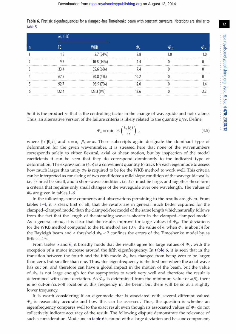
12

rspa.royalsocietypublishing.orgProc.R.Soc.A470:20130718

...................................................

Table 6. First six eigenfrequencies for a clamped-free Timoshenko beam with constant curvature. Notations are similar totable 5.

ωn (Hz)

n FE WKB Φu Φβ Φw

1 1.8 2.7 (54%) 2.8 1.0 1.0. . . . . . . . . . . . . . . . . . . . . . . . . . . . . . . . . . . . . . . . . . . . . . . . . . . . . . . . . . . . . . . . . . . . . . . . . . . . . . . . . . . . . . . . . . . . . . . . . . . . . . . . . . . . . . . . . . . . . . . . . . . . . . . . . . . . . . . . . . . . . . . . . . . . . . . . . . . . . . . . . . . . . . . . . . . . . . . . . . . . . . . . . . . . . . . . . . . . . . . . . .

2 9.5 10.8 (14%) 4.4 0 0. . . . . . . . . . . . . . . . . . . . . . . . . . . . . . . . . . . . . . . . . . . . . . . . . . . . . . . . . . . . . . . . . . . . . . . . . . . . . . . . . . . . . . . . . . . . . . . . . . . . . . . . . . . . . . . . . . . . . . . . . . . . . . . . . . . . . . . . . . . . . . . . . . . . . . . . . . . . . . . . . . . . . . . . . . . . . . . . . . . . . . . . . . . . . . . . . . . . . . . . . .

3 33.4 35.6 (6%) 7.4 0 0. . . . . . . . . . . . . . . . . . . . . . . . . . . . . . . . . . . . . . . . . . . . . . . . . . . . . . . . . . . . . . . . . . . . . . . . . . . . . . . . . . . . . . . . . . . . . . . . . . . . . . . . . . . . . . . . . . . . . . . . . . . . . . . . . . . . . . . . . . . . . . . . . . . . . . . . . . . . . . . . . . . . . . . . . . . . . . . . . . . . . . . . . . . . . . . . . . . . . . . . . .

4 67.5 70.8 (5%) 10.2 0 0. . . . . . . . . . . . . . . . . . . . . . . . . . . . . . . . . . . . . . . . . . . . . . . . . . . . . . . . . . . . . . . . . . . . . . . . . . . . . . . . . . . . . . . . . . . . . . . . . . . . . . . . . . . . . . . . . . . . . . . . . . . . . . . . . . . . . . . . . . . . . . . . . . . . . . . . . . . . . . . . . . . . . . . . . . . . . . . . . . . . . . . . . . . . . . . . . . . . . . . . . .

5 92.7 98.9 (7%) 12.0 0 1.4. . . . . . . . . . . . . . . . . . . . . . . . . . . . . . . . . . . . . . . . . . . . . . . . . . . . . . . . . . . . . . . . . . . . . . . . . . . . . . . . . . . . . . . . . . . . . . . . . . . . . . . . . . . . . . . . . . . . . . . . . . . . . . . . . . . . . . . . . . . . . . . . . . . . . . . . . . . . . . . . . . . . . . . . . . . . . . . . . . . . . . . . . . . . . . . . . . . . . . . . . .

6 122.4 123.3 (1%) 13.6 0 2.2. . . . . . . . . . . . . . . . . . . . . . . . . . . . . . . . . . . . . . . . . . . . . . . . . . . . . . . . . . . . . . . . . . . . . . . . . . . . . . . . . . . . . . . . . . . . . . . . . . . . . . . . . . . . . . . . . . . . . . . . . . . . . . . . . . . . . . . . . . . . . . . . . . . . . . . . . . . . . . . . . . . . . . . . . . . . . . . . . . . . . . . . . . . . . . . . . . . . . . . . . .

So it is the product rε that is the controlling factor in the change of waveguide and not ε alone.Thus, an alternative version of the failure criteria is likely related to the quantity k/rε. Define

Φx = min∣∣∣∣

(kx(ξ )εr

)∣∣∣∣ , (4.5)

where ξ ∈]0, L[ and x = u, β, or w. These subscripts again designate the dominant type ofdeformation for the given wavenumber. It is stressed here that none of the wavenumberscorresponds solely to either flexural, axial or shear motion, but by inspection of the modalcoefficients it can be seen that they do correspond dominantly to the indicated type ofdeformation. The expression in (4.5) is a convenient quantity to track for each eigenmode to assesshow much larger than unity Φx is required to be for the WKB method to work well. This criteriacan be interpreted as consisting of two conditions: a mild slope condition of the waveguide walls,i.e. εr must be small, and a short-wave condition, i.e. k/ε must be large, and together these forma criteria that requires only small changes of the waveguide over one wavelength. The values ofΦx are given in tables 1–6.

In the following, some comments and observations pertaining to the results are given. Fromtables 1–4, it is clear, first of all, that the results are in general much better captured for theclamped–clamped model than the clamped-free model of the same length which naturally followsfrom the fact that the length of the standing wave is shorter in the clamped–clamped model.As a general trend, it is clear that the results improve for large values of Φu. The deviationsfor the WKB method compared to the FE method are 10%, the value of ε, when Φu is about 4 forthe Rayleigh beam and a threshold Φu < 2 confines the errors of the Timoshenko model by aslittle as 4%.

From tables 5 and 6, it broadly holds that the results agree for large values of Φx, with theexception of a minor increase around the fifth eigenfrequency. In table 6, it is seen that in thetransition between the fourth and the fifth mode Φw has changed from being zero to be largerthan zero, but smaller than one. Thus, this eigenfrequency is the first one where the axial wavehas cut on, and therefore can have a global impact in the motion of the beam, but the valueof Φw is not large enough for the asymptotics to work very well and therefore the result isdetermined with some deviation. As Φw is determined from the minimum value of k(S), thereis no cut-on/cut-off location at this frequency in the beam, but there will be so at a slightlylower frequency.

It is worth considering if an eigenmode that is associated with several different valuedΦx is reasonably accurate and how this can be assessed. Thus, the question is whether aneigenfrequency compares well to the exact result even though its associated values of Φx do notcollectively indicate accuracy of the result. The following dispute demonstrate the relevance ofsuch a consideration. Mode one in table 6 is found with a large deviation and has one component,

on August 13, 2014rspa.royalsocietypublishing.orgDownloaded from

13

rspa.royalsocietypublishing.orgProc.R.Soc.A470:20130718

...................................................

0.8

0.6

0.4

0.2

0.5 1.0S

1.5 2.0

Figure 2. Mode shapes for clamped-free curved Timoshenko beam, first mode. Solid line, u(S); dotted line,β(S); dashed line,w(S).

1.0

0.8

0.6

0.4

0.2

–0.20.5 1.0 1.5 2.0

S

Figure 3. Mode shapes for clamped–clamped curved Timoshenko beam, thirdmode. Solid line, u(S); dotted line,β(S); dashedline,w(S).

Φu > 2, which suggests that it is probably accurate, whereas the two others, Φβ < 2 and Φw < 2,suggest that it is not very accurate. Contrary, mode three in table 5 is found with a small deviation,but Φw suggests that it is wrong while Φu suggests that it is correct. The disagreement has asimple explanation that becomes evident by plotting the actual mode shapes. These are seen infigures 2 and 3. Here, it is seen in figure 3 that mode three is dominated by flexural motion,u(S), and the fact that the value of Φw suggests the mode is outside the WKB validity rangeis therefore not relevant. From figure 2, it is clear that axial motion cannot be neglected whencompared with flexural motion and therefore the approximation fails. In other words, the measureof ‘asymptoticness’, Φx, needs to be accompanied by an assessment of the involvement of modesfor multi-modal problems. This involvement of modes can possibly be further quantified by themodal participation factor known from forced vibration [16]. Finally, it is seen that clampingboth ends of the curved Timoshenko beam drastically increases the first eigenfrequency whencompared with its cantilevered counterpart. This has a simple physical explanation: the bendingcouples to stretching due to the curvature, but stretching resistance is high since the beam isclamped at both ends.

A comparison of dispersion relationships is shown in appendix A in which the Rayleigh andTimoshenko rod theories are compared to the Pochhammer–Chree elastodynamics solution forwaves in a straight elastic rod with circular cross section. The comparison demonstrates thatTimoshenko theory for the parameters chosen can be expected to work well until about 8 kHz,

on August 13, 2014rspa.royalsocietypublishing.orgDownloaded from

14

rspa.royalsocietypublishing.orgProc.R.Soc.A470:20130718

...................................................

Table 7. Percentage deviations between WKB and FE of the first eigenfrequency for a clamped–clamped Rayleigh beam inthe ε–r parameter space. Short dashed lines boundsΦu < π , medium dashed lines boundsΦu < 2 and long dashed linesboundsΦu < 1.

ε (%)

r 0.001 0.01 0.02 0.03 0.04 0.05 0.06 0.07 0.08 0.09. . . . . . . . . . . . . . . . . . . . . . . . . . . . . . . . . . . . . . . . . . . . . . . . . . . . . . . . . . . . . . . . . . . . . . . . . . . . . . . . . . . . . . . . . . . . . . . . . . . . . . . . . . . . . . . . . . . . . . . . . . . . . . . . . . . . . . . . . . . . . . . . . . . . . . . . . . . . . . . . . . . . . . . . . . . . . . . . . . . . . . . . . . . . . . . . . . . . . . . . . .

0.001 0 0 0 0 1 0 1 0 0 0

0.1 0 0 0 0 0 0 1 1 1 2

0.2 0 0 0 0 1 0 1 2 2 3

0.3 0 0 0 0 0 1 1 2 3 4

0.4 0 0 0 0 0 1 2 3 4 5

0.5 0 0 0 0 1 1 2 3 4 6

0.6 0 0 0 0 1 1 2 3 5 7

0.7 0 0 0 0 1 1 2 4 5 7

0.8 0 0 0 0 1 1 2 4 6 8

0.9 0 0 0 0 1 1 3 4 6 9ε (%)

r 0.1 0.2 0.3 0.4 0.5 0.6 0.7 0.8 0.9 1. . . . . . . . . . . . . . . . . . . . . . . . . . . . . . . . . . . . . . . . . . . . . . . . . . . . . . . . . . . . . . . . . . . . . . . . . . . . . . . . . . . . . . . . . . . . . . . . . . . . . . . . . . . . . . . . . . . . . . . . . . . . . . . . . . . . . . . . . . . . . . . . . . . . . . . . . . . . . . . . . . . . . . . . . . . . . . . . . . . . . . . . . . . . . . . . . . . . . . . . . .

0.001 0 0 1 0 0 1 0 0 0 0

0.1 2 7 2 −5 1 3 −6 −5 2 −2

0.2 4 13 4 −10 2 4 −10 −9 7 0

0.3 5 19 7 −15 4 4 −12 −11 17 5

0.4 6 25 10 −18 5 5 −14 −13 34 18

0.5 8 32 13 −21 5 6 −14 −12 63 40

0.6 9 39 17 −23 7 11 −11 −11 114 77

0.7 10 47 17 −23 11 22 −2 −6 185 162

0.8 11 56 11 −27 28 58 22 11 422 354

0.9 12 69 159 76 324 612 464 378 3429 14 042. . . . . . . . . . . . . . . . . . . . . . . . . . . . . . . . . . . . . . . . . . . . . . . . . . . . . . . . . . . . . . . . . . . . . . . . . . . . . . . . . . . . . . . . . . . . . . . . . . . . . . . . . . . . . . . . . . . . . . . . . . . . . . . . . . . . . . . . . . . . . . . . . . . . . . . . . . . . . . . . . . . . . . . . . . . . . . . . . . . . . . . . . . . . . . . . . . . . . . . . . .

whereas the Rayleigh theory breaks down at a much earlier stage. In fact, it can be observed fromthe results in tables 1 and 3 that already at the sixth eigenfrequency the Rayleigh theory divergesby 17% from the Timoshenko theory.

The attention is now turned to an inspection of how the results compare in the ε − r parameterspace—the two parameters free to choose in the modulation of the waveguide with the givenfunctional form of d(s). In table 7 is the deviation between WKB method and FE method shown forthe first eigenfrequency for a clamped–clamped Rayleigh beam at various combination of ε and r.Level curves are drawn in the table that bounds Φu less than π , 2, and 1. It can be observed fromthe results in table 7 that none of the level curves perfectly captures the incorrect results. Thus,it is not possible to state a minimum value of Φu, but only require that Φu 1. It is observed,however, that in many cases Φu > 3 is actually sufficient. Additionally, it is pointed out that themeasure for validity proposed in this paper, equation (4.5), correctly predicts that, results basedon a large value of ε, but a small value of r, and vice versa, can be determined correctly. This is animprovement compared to the more traditional measure in (4.3).

on August 13, 2014rspa.royalsocietypublishing.orgDownloaded from

15

rspa.royalsocietypublishing.orgProc.R.Soc.A470:20130718

...................................................

6

5

4

3

2

1

02000 4000 6000 8000

w*, (Hz)10 000 12 000 14 000

Re(

k*),

(m

–1)

Figure 4. Dispersion diagram for straight rod with circular cross section. Dotted curves, Pochhammer–Chree solution ofelastodynamics; solid lines, Timoshenko theory; dashed lines, Rayleigh theory. The plot is generated with the parametersintroduced in §4, but for a constant cross section, i.e. r = 0. The two Pochhammer–Chree branches that are not accompaniedby a Rayleigh or a Timoshenko branch corresponds to axial and torsional wave motion.

5. ConclusionIn the work presented in this paper, the WKB method is applied to approximate the solution ofthe wave propagation problem in non-uniform beams. It is demonstrated that the leading orderWKB approximation corresponds to conservation of energy flux. The solutions are specializedto clamped–clamped and clamped-free boundary conditions, and a number of eigenfrequenciesare determined and compared to those determined by the FE method. A parameter study isconducted and the validity range of the WKB method and the plane cross-sectional hypothesisare discussed. It is found that min |(k(ξ )/εr)| 1 is a conservative criterion for accuratedetermination of an eigenfrequency by the WKB method. It is furthermore illustrated thatoften min |(k(ξ )/εr)| > 3 is sufficient. For multi-modal problems, this criterion needs to beaccompanied by an assessment of what kind of motion is dominant for a given mode. This can beconducted by investigating the mode shape.

It is found that there is an appreciable overlap of validity between the WKB method andTimoshenko beam theory, the overlap with Rayleigh (or Bernoulli–Euler) beam theory is found tobe much more narrow.

The simplicity of the WKB approximation, and the fact that the dispersion relation matchesthat of the unperturbed waveguide, illustrates the power of the method in the analysis of non-uniform rods. This is fortunate as the wavenumbers often will be known a priori; these arejust the same as the wavenumbers found for the corresponding uniform waveguide. It seemsnatural to extend the analysis to waveguides with constant cross section, but varying curvature.These kind of structures are of practical interest in the analysis of the linear time harmonicdynamics of suspension systems, pipes, curved rails, etc., where one would be concerned withnoise transmission and energy flux. Since the ‘standard’ WKB approximations reported in thispaper, as is shown, conserves the energy flux it seems obvious to propose to analyse turningpoint problems. Doing so allows to study problems where the net energy flux is zero because ofthe wave reflection at a turning point. This will give detailed information on the internal reflection

on August 13, 2014rspa.royalsocietypublishing.orgDownloaded from

16

rspa.royalsocietypublishing.orgProc.R.Soc.A470:20130718

...................................................

of waves in a non-uniform beam structure and can potentially be used to analyse asymptoticallystop and pass bands in rods with periodic curvature.

Acknowledgements. The authors address their sincere gratitude to Prof. C. J. Chapman for the many discussionson the topic.Funding statement. The research is funded by The Danish Council for Independent Research, Technology and

Production Sciences.

Appendix A. Comparison of rod theories and elastodynamicsHere, the validity ranges of the Rayleigh beam theory and the Timoshenko beam theory aredemonstrated and discussed briefly. In figure 4, the dispersion diagram for a beam in terms of theRayleigh beam model, the Timoshenko beam model and the Pochhammer–Chree exact solutionof elastodynamics is shown. For details on the Pochhammer–Chree solution, see Chree [17]. Theplot illustrates how well the first branch of the Timoshenko model compares to the Pochhammer–Chree solution in a large frequency range (until ω∗ ≈ 14 kHz corresponding to ω ≈ 3), whereas theRayleigh model compares well only at much lower frequencies. There is an obvious mismatchbetween Timoshenko theory and Pochhammer–Chree when it comes to the second branch (theshear wave). This is not of any great importance for frequencies lower than this cut-on frequencyas the shear wave in this regions is evanescent. It should be mentioned that the cut-on canbe perfectly matched with a proper selection of λ. For the non-uniform Timoshenko beams,the lowest cut-on is found to be ω∗ ≈ 8 kHz for both the straight and curved beam modelwith the parameters in §4. The disagreement between Rayleigh and Timoshenko model caneven be observed by comparing the results in, for instance, tables 1 and 3. Here, the deviationbetween the Rayleigh results and the Timoshenko results is about 17% already at the sixtheigenfrequency.

References1. Fröman N, Fröman PO. 2004 Physical problems solved by the phase-integral method. Cambridge,

UK: Cambridge University Press.2. Bender CM, Orszag SA. 1978 Advanced mathematical methods for scientists and engineers. New

York, NY: McGraw-Hill.3. Rienstra SW. 1999 Sound transmission in slowly varying circular annular lined ducts with

flow. J. Fluid Mech. 380, 279–296. (doi:10.1017/S0022112098003607)4. Cooper AJ, Peake N. 2001 Propagation of unsteady disturbances in a slowly varying duct with

mean swirling flow. J. Fluid Mech. 445, 207–234. (doi:10.1017/S0022112001005559)5. Brambley EJ, Peake N. 2008 Sound transmission in strongly curved slowly varying cylindrical

ducts with flow. J. Fluid Mech. 596, 387–412. (doi:10.1017/S0022112007009603)6. Scott JFM, Woodhouse J. 1992 Vibration of an elastic strip with varying curvature. Phil. Trans.

R. Soc. Lond. A 339, 587–625. (doi:10.1098/rsta.1992.0052)7. Gridin D, Craster RV, Fong J, Lowe MJS, Beard M. 2003 The high-frequency

asymptotic analysis of guided waves in circular elastic annulus. Wave Motion 38, 67–90.(doi:10.1016/S0165-2125(03)00002-7)

8. Rosenfeld G, Keller JB. 1975 Wave propagation in nonuniform elastic rods. Acoust. Soc. Am.57, 1094–1096. (doi:10.1121/1.380558)

9. Pierce AD. 1970 Physical interpretation of the WKB or eikonal approximation for wavesand vibrations in inhomogeneous beams and plates. Acoust. Soc. Am. 48, 275–284.(doi:10.1121/1.1912125)

10. Langley R. 1999 Wave evolution, reflection, and transmission along inhomogeneouswaveguides. J. Sound Vib. 227, 131–158. (doi:10.1006/jsvi.1999.2337)

11. Sorokin SV, Chapman CJ. 2011 A hierarchy of rational Timoshenko dispersion relations.J. Sound Vib. 330, 5460–5473. (doi:10.1016/j.jsv2011.06.004)

on August 13, 2014rspa.royalsocietypublishing.orgDownloaded from

17

rspa.royalsocietypublishing.orgProc.R.Soc.A470:20130718

...................................................

12. Shames IH, Dym CL. 1991 Energy and finite element methods in structural mechanics. London,UK: Taylor & Francis.

13. Rayleigh JWS. 1945 The theory of sound. New York, NY: Dover Publications.14. Chapman CJ, Sorokin SV. 2010 The finite-product method in the theory of waves and stability.

Proc. R. Soc. A 466, 471–491. (doi:10.1098/rspa.2009.0255)15. Hinch EJ. 1991 Perturbation methods. Cambridge, UK: Cambridge University Press.16. Rao S. 2004 Mechanical vibrations. Englewood Cliffs, NJ: Prentice Hall.17. Chree C. 1889 The equations of an isotropic elastic solid in polar and cylindrical coordinates,

their solutions and applications. Trans. Camb. Philos. Soc. 14, 250–309.

on August 13, 2014rspa.royalsocietypublishing.orgDownloaded from

Paper 2

Nielsen R.B, Peake N. (to be submitted): ”Tunnelling effects of waves in acousticflow ducts” Journal of Sound and Vibration

47

PAPER 2

48

Tunnelling effects of acoustic waves in slowly varying

axisymmetric flow ducts

R.B. Nielsena, N. Peakeb

aDepartment of Mechanical and Manufacturing Engineering, Aalborg University,Fibigerstraede 16, 9220 Aalborg, Denmark

bDepartment of Applied Mathematics and Theoretical Physics, University of Cambridge,Wilberforce Road, CB3 0WA, United Kingdom

Abstract

The multiple-scales Wentzel-Kramers-Brillouin (WKB) approximation is ap-plied to model the propagation of acoustic waves in an axisymmetric flowduct with a constriction. An analysis of the reflection/transmission processof modes tunnelling through the constriction is conducted. The resultingpiecewise solution consists of WKB solutions in regions away from the con-striction and a solution valid in the near vicinity of it. A complementaryapproach is demonstrated hereafter and a uniformly valid solution is de-rived. The solutions are demonstrated through two test cases, one with andone without a mean flow. The effect of tunnelling is illustrated and thecorrespondence between the piecewise and the uniform solution is shown.

Keywords: Non-uniform acoustic duct, tunnelling effects, turning pointanalysis, uniformly valid solution

1. Introduction

The interest in reducing noise emission from machinery such as aircraftengines have resulted in a considerable effort payed to study sound trans-mission through slowly varying flow ducts. Consequently, a vast numberof alterations of such waveguide studies are currently available. A smallselection of these are: Circular lined ducts with a mean flow [1], ducts ofarbitrary cross section with a mean flow [2], ducts with a mean swirling flow

Email address: rn@m-tech.aau.dk (R.B. Nielsen)

Preprint submitted to Journal of Sound and Vibration March 23, 2015

[3], and strongly curved ducts [4]. In these papers formulae for wavenumbersand amplitudes are derived using the Wentzel-Kramers-Brillouin (WKB) ap-proximation which is applicable when the duct variation is small over a wavelength. An analysis of modes undergoing a transition from cut-on to cut-offin the duct is often included and reveals that an incident wave is fully re-flected with a phase shift −π/2 at the transition point. Consequently onlyan evanescent wave is transmitted beyond the transition point and the netenergy flux of the mode therefore vanishes. This effect of internal wave re-flection is advantageous from a noise reduction perspective and is the mainfocus of this paper.

The singular transition points in acoustics are analog to the turning pointsoccurring in solutions to the Schrodingers equation which have been stud-ied intensively. A parabolic potential with two turning points is treated in[5] and expressions for reflection and transmission coefficients depending onthe distance between the turning points was derived. Keller [5] furthermorederived a uniformly valid approximation for a general potential with twoturning points.From this uniformly valid solution reflection and transmissioncoefficients can be extracted. By such a solution one avoids the tedious pro-cess of matching inner and outer solutions in overlap regions which contraststhe more traditional procedure available from [6] or [7].

The concept of uniformly valid solutions have been employed in flow ductacoustics before. In [8] a uniformly valid solution for modes undergoing acut-on cut-off transition in a hard-walled acoustic duct of arbitrary cross sec-tion with a irrotational mean flow was derived. It does not seem, however,that the acoustic duct analogy of the work by Keller [5] has been attempted.The focus of this paper is specifically to apply the WKB method to model thewave propagation in an acoustic duct with two turning points and therebydetermine the inner and outer solution and the corresponding uniform solu-tion.

The description of the acoustic field using eigenmodes is attractive sincethese form a complete basis from where any solution may be represented bysummation of these eigenmodes. The results from previous publications allowonly modes that remains cut-on through out the duct and those that is fullyreflected at a transition point to be accounted for. The effect of a mode thatcuts off and cuts on again slightly further downstream can therefore not beaccounted for yet. Having such results available would help engineers in thedesign process of aircraft engines when analysing the noise transmission fromthe fan to the surroundings. The result may furthermore serve as benchmark

2

solutions for computational aeroacoustic codes.This paper focuses on the reflection and transmission of modes tunnelling

through a cut-on cut-off cut-on region of a slowly varying cylindrical hard-walled duct with an irrotational mean flow. The analysis is presented in thefollowing order. In Section 2 the equations governing the flow and acousticfield are presented. The slowly varying modes, i.e. those that are either wellcut-on or those far away from the transition points are derived in Section3. In Section 4 the wave motion through the neck of the duct is studiedand by asymptotic matching to the outer solution reflection and transmissioncoefficients are determined. Lastly, a uniform approximation is derived whichis valid both far up- and downstream as well as in close proximity of thetransition points. This derivation is presented in Section 5. The resultsare finally presented through a collection of test cases in Section 6. Here theeffect of tunnelling is illustrated and the correspondence between the uniformsolution and the piecewise solution is shown.

2. Problem formulation

The setup of the problem largely follows that of [8] and the similar nota-tion is therefore adopted. The duct is defined as hard-walled and circular, andthe flow and sound field enters the duct from each side as indicated in Figure1. The acoustic medium is assumed to be a compressible inviscid isentropicirrotational gas. In what follows we non-dimensionalise distances by the farupstream radius R∞, speeds and density by c∞ and ρ∞, respectively. Let,

xt=0

2xa

2xa

2xa

Inner region

xRegion IRegion II

xr

θ

n

Acoustic field

R(x)

Inlet

Figure 1: Illustration of a duct with a constriction. The flow is assumed to enter the ductfrom the right hand side and the acoustic field is assumed to enter from the left hand side.

with no loss of generality, the neck of the duct be located symmetrically aboutx = 0 for convenience. The duct is assumed to be slowly varying, that is theratio between the local crosswise length scale R∞, compared to the lengthscale over which the duct geometry changes l is small, i.e. ε = R∞/l << 1.Thus, on a slow scale defined as X = εx the radius varies like R(X).

3

The flow field is split into a stationary mean flow and small time-harmonicperturbations [1]

[v, ρ, p, c] = [V, D, P, C] + [∇φ, ρ, p, c] e−iωt (1)

where v designate the velocity field and p is the pressure. The equationsgoverning the flow field are [9]

0 =∂ρ

∂t+∇ · (ρv) (2)

0 = ρ

(∂v

∂t+ v · ∇v

)+∇p (3)

c2 = ργ−1 (4)

γp = ργ (5)

where γ is the ratio of specific heats. With the introduction of the velocitypotential φ pressure and density perturbations can be eliminated and theconvected wave equation emerges

∇ · (D∇φ)−D (−iω + V · ∇)

[1

C2(−iω + V · ∇)φ

]= 0 (6)

A time dependence e−iωt has been adopted. For a hard-walled duct withoutward pointing normal n the boundary conditions are

∇φ · n = 0 (7)

The steady mean flow component can according to [1] be expanded by

V(X, r, θ) = U0(X)ex + εV1(X, r)er +O(ε2) (8)

D(X, r) = D0(X) +O(ε2) (9)

C(X, r) = C0(X) +O(ε2) (10)

P (X, r) = P0(X) +O(ε2) (11)

where V1 denotes a radial flow. The leading order mean flow componentscan be determined from Bernoulli’s equation, mass flux conservation, andequation (4) and (5). A slowly varying solution to equation (6) is derived inthe following subsection.

4

3. The slowly varying modes

Due to the circular cross-section the solution will be of Fourier-WKBform, specifically we assume

φ ∼(Φ0 + εΦ1 +O(ε2)

)e

iε

∫X k(X′)dX′−imθ, as ε→ 0 (12)

Inserting this in (6) and collecting terms of O(1) yields the Bessel equation

∂2Φ0

∂r2+

1

r

∂Φ0

∂r+

((ω − kU0)2

C20

− k2 − m2

r2

)Φ0 = 0 (13)

where m and k are the circumferential and axial wavenumbers, respectively.The O(1) boundary condition becomes

∂Φ0

∂r= 0 on r = R(X) (14)

with the introduction of Φ0 = N(X)ψ(r;X) we have

ψ = b1Jm(αr) (15)

where b1 is an arbitrary constant to be determined from the sound sourceand α =

µjR(X)

with µj being a root of J ′m(µj) = 0. A term proportional

to the Bessel function of the second kind has been omitted in (15) to re-move the singularity at r = 0. From the O(1) boundary condition the axialwavenumber is determined

k =−ωU0

C20 − U2

0

± ωC0σ

C20 − U2

0

(16)

in which σ is the reduced wavenumber

σ =

√1− (C2

0 − U20 )α2

ω2(17)

The unknown axially varying amplitude N(X) is obtainable from a solv-ability condition determined from the O(ε) terms in the convected wave equa-tion. After some manipulation and the application of the steady mass con-servation condition

∂

∂X(D0U0) = −D0

r

∂

∂r(rV1) (18)

5

one arrives at the following O(ε) terms

∂2Φ1

∂r2+

1

r

∂Φ1

∂r+

((ω − kU0)2

C20

− k2 − m2

r2

)Φ1 =

− i

Φ0

∂

∂X

[((ω − kU0)U0

C20

+ k

)D0Φ2

0

]+

1

r

∂

∂r

[rV1

ω − kU0

C20

D0Φ20

](19)

with O(ε) boundary conditions

∂Φ1

∂r+ ikR′Φ0 = 0 on r = R(X) (20)

To leave the solvability condition on Φ0 only multiply (19) with Φ0 andintegrate over the duct cross section. After the use of the O(ε) boundarycondition, the mean flow equations to eliminate V1, and Leibniz rule onearrives at the adiabatic invariant

i

N

d

dX

[ωσD0R

2

C0

N2

]= 0 (21)

Thus, we conclude that, apart from a multiplicative constant, N(X) is

N(X) =

√C0(X)

ωσ(X)D0(X)R2(X)(22)

The outer solution, i.e. away from prospective transition points, is found bysummation of modes of the following form

φj =

√C0(X)

ωσ(X)D0(X)R2(X)Jm

(µk

R(X)r

)e−imθe

− iε

∫X′ ωU0C20−U

20

dX′

β1e

iε

∫X′ ωC0σ

C20−U

20

dX′+ β2e

− iε

∫X′ ωC0σ

C20−U

20

dX′

(23)

With the designations T , I and R representing transmitted, incident, andreflected waves, respectively, the solutions are stated as: β1 = T and β2 = 0to the right of the neck, and by: β2 = I and β1 = R to the left of the neck.We note, furthermore, that at a turning point, i.e. when σ(X) is zero N(X),becomes infinite and the solution breaks down. This case is treated in thenext section.

6

4. Turning point analysis

The singular behavior of the transport equation (21) at a turning point isdue to the neglect of higher order terms that become significant when Φ0(X)changes rapidly. The most rapidly varying O(ε2) term is

D0

(1− U2

0

C20

)∂2Φ0

∂X2(24)

Thus, promoting this term to the transport equation removes the singularbehavior. First, add (24) to (19), multiply with Φ0(X), and then integrationover the cross section yields

id

dX

[ωσD0R

2

C0

N2(X)

]+ εR2D0

(1− U2

0

C20

)N(X)

d2N(X)

dX2= 0 (25)

We shall now consider the behavior of the reduced wavenumber in order tointroduce an appropriate inner scale that balances the terms in (25) as ε→ 0.Close to the neck we expand the reduced wavenumber by

σ2 ∼ A2(X2 − b) as X → 0 (26)

The parameter b is real, but may be positive, zero or negative representingthe cases of two real turning points, a double turning point, or two complexturning points, respectively. Now we introduce a scaled inner coordinate X =εqX. Selecting q = −1/2 ensures that the higher order term in (25) becomesas significant as the original terms in the transport equation. Furthermore,do we introduce a scaled version of b, b = εb, which ensures b is as significantas X2 in the expansion of σ2. Thus, the turning points (Xt = ±

√b) are

necessarily located on X. The transport equation becomes

d2B

dX2+

(ωC0

C20 − U2

0

)2

A2(X2 − b

)B = 0 (27)

Where the following substitution has been made

N(X) = B(X)e− iε

∫X0

ωc0σ

C20−U

20

dX′(28)

to reduce the equation to standard form. One may remark that derivativesof any slowly varying quantity (U0, C0, D0, or R) are roughly constant on

7

the inner scale and therefore should be ignored. Further reduction of (27) isdone by the two parameters

z = X

√2A

ωC0

C20 − U2

0

(29)

a =Ab

2

ωC0

C20 − U2

0

(30)

we then arrive at

d2B

dz2+

(z2

4− a)B = 0 (31)

This is the Parabolic Cylinder Equation and has the solution [10]

B = c1W (a, z) + c2W (a,−z) (32)

where c1 and c2 are arbitrary constants to be determined from matchingwhich is done by comparing the inner and outer solutions when these areexpanded in the appropriate limits. The outer solution in the transmissionregion when X approaches the transition point is written as:

φT ∼[√

C0

ωD0R2

]

X=Xt

TA1/2X1/2

eiε

ωC0C20−U

20

A2X2−ia

2−ia ln

(2X√b

)

as X →√b

(33)

Here we have omitted the Bessel-Fourier and convected part of the solutionas this appear similarly on both inner and outer solution. This result isobtainable through the application of an intermediate variable Y = X/εη

with 0 < η < 1/2 to neglect small phase shifts due to the smallness of ε.The appropriate expansions of W (a, z) for large positive and negative

arguments are available in [10]. For z →∞ the result is

φinner ∼[c1

√k

2z− ic2

√1

2kz

]eiΩ +

[c1

√k

2z+ ic2

√1

2kz

]e−iΩ (34)

where

Ω = 14z2 − a ln(z) + 1

4π + 1

2φ2 (35)

φ2 = 6 Γ(

12

+ ia)

(36)

k =√

1 + e2πa − eπa (37)

8

At this intermediate step we are in a position to choose c2 = ikc1 to eliminatethe left going wave. Rewriting the inner solution in terms of the outer variableX yields

φinner ∼c1k21/4

(ωC0

C20−U2

0

)1/4 (Aε

)1/4X1/2

eiε

ωC0C20−U

20

A2X2−ia ln

(2X√b

)−ia

2ln(|a|)+iπ

4+i

φ22 (38)

as X →∞ (39)

By comparing terms in the inner and outer solutions and perform the sim-ilar expansions upstream from the constriction three additional matchingconditions are found. The solutions to these are:

TI =

eia−ia ln|a|+iφ2

√1 + e2aπ

(40)

RI =

eπaeia−ia ln|a|+iφ2−iπ/2

√1 + e2aπ

(41)

c1

I =

[√C0

ωD0

(ωC0

C20 − U2

0

)1/4]

X=Xt

(8

εA

)1/4k1/2

i(1 + k2

)ei(−a2 ln|a|+a2

+π4

+φ22 )

(42)

c2 = ikc1 (43)

The velocity potential in the inner region is finally given by

φinner = (c1W (a, z) + c2W (a,−z)) Jm

(µ

R(X)r

)e

iε

∫∞0

−ωU0C20−U

20

dX′−imθ(44)

The solution derived in the this section consists of WKB solutions in theouter regions and the above solution in the inner region shall henceforth bereferred to as a composite solution. In the next section we derive a solutionvalid at any location, i.e. a uniform solution.

5. Uniform solution

The derivation of a uniformly valid solution can be conducted from theleading order terms of (6) when the mean flow is assumed to be slowly vary-ing. These are, see [2]:

(1− U0

C0

)∂2φ

∂x2+

2iωU0

C20

∂φ

∂x+

(ω2

C20

− α2

)φ = O(ε) (45)

9

Again this is reducible to:

∂2φ

∂x2+ k2

2φ = O(ε) (46)

with the substitution:

φ = φe−i∫ U0ω

C20−U

20

dx(47)

and k2 = ωC0σC2

0−U20. Guided by [5] and [8] we shall seek a solution of the form

φ = Φ(X, r, θ)G(ζ)

(ζx)1/2

(48)

where ζ(x) is a function to be determined. We assume initially that itsderivative ζx varies slowly. Immediately it is noticed that due to the neglectof higher order terms the second derivative of φ is

∂2φ

∂x2= G′′ (ζx)

3/2 Φ(X, r, θ) (49)

where primes denote derivatives wrt. ζ. Applying this in (46) yields

(G′′ +

k22

ζ2x

G

)Φ(X, r, θ) = 0 (50)

By dropping the slowly varying Φ this becomes the parabolic cylinder equa-tion provided that we select

ζ2x

(ζ2

4− η)

= k22 (51)

with ζ as the argument and η as a parameter corresponding to a in equation(31). Once again, the solution can be stated by summation of paraboliccylinder functions:

G(ζ) = h1W (η, ζ) + h2W (η,−ζ) (52)

but the relation between ζ and x remains unknown at this stage. To deter-mine this relation we eliminate ζx in (51) which can be done by integration.At two real turning points located at x = x0,1 we have k2

2 = 0 corresponding

10

to ζ(x0) = −2√η and ζ(x1) = 2

√η with η > 0. So equation (51) in the

downstream region x > x1 becomes

ζ

4

√ζ2 − 4η − η ln

[ζ +

√ζ2 − 4η

2η

]=

∫ x

x1

k2dx (53)

In the tunnelling region x0 < x < x1 we find

ζ

4

√4η − ζ2 + η sin−1

(ζ

2√η

)+πη

4=

∫ x

x0

|k2|dx (54)

By selecting ζ(x1) = 2√η in this equation yields

πη =

∫ x1

x0

|k2|dx (55)

Which determines η. In the upstream region x < x0 we get:

ζ

4

√ζ2 − 4η + η ln

[−ζ +

√ζ2 − 4η

2η

]=

∫ x

x0

k2dx (56)

Similarly, when η < 0 the turning points are complex and we have k22 =

0 at x0,1 where Im(x0,1) 6= 0, so at these locations ζ(x0) = −2i|η|1/2 andζ(x1) = 2i|η|1/2. By eliminating ζx in equation (51) yields:

ζ

4

√ζ2 + 4|η|+ |η| ln

(ζ +

√ζ2 + 4|η|

2|η|1/2

)=

∫ x

0

kdx (57)

for any x. Furthermore, do we find:

π|η| =∫ Im(x1)

Im(x0)

k(is)ds (58)

The unknown η can now be determined from equation (55) and (58),while ζ is obtained by solving equation (53), (54), and (56) for η > 0 andequation (57) for η < 0, at each axial station. This naturally entails numericalintegration of k in these equation and subsequent numerically solving for ζwhich is straight forward in all cases. ζx is subsequently determined fromequation (51).

11

The constants h1 and h2, and the function Φ(X, r, θ) can now be de-termined. Similar to the analysis in section 4 do we require no left goingwave downstream from the constriction and therefore h2 = ikh1. To fix theincident wave to be the same as the upstream WKB solution we select:

h1Φ(X, r, θ) =2√kI

k2 + 1

√C2

0

D0(C20 − U2

0 )R2e−imθJm(αr)e−

iη2

ln(η)+iη2− iπ

4+

iφ22

(59)

This result is obtainable by expanding the parabolic cylinder functions inequation (52) for large negative arguments and compare to (23). This con-cludes the derivation of the uniform solution.

6. Results

Before turning to specific test cases the behaviour of T andR as a→ ±∞and a → 0 is examined. From Stirling’s formula is it found that φ2 ∼a ln |a| − a as a→∞. For large tunnelling distances it is found from (40)and (41) that

∣∣TI∣∣ → 0 and

∣∣RI∣∣ → 1. In the a → −∞ these are reversed.

The phase changes are 6 TI → 0 and 6 RI → −π2

as a → ±∞. I.e. for largetunnelling distances the result becomes what is known from the well-knownone turning point problem, namely a fully reflected wave with a −π

2phase

shift. If a = 0 then∣∣TI∣∣ =

∣∣RI∣∣ = 1√

2. Thus, when the two transitions points

merge half the energy of the incident wave is transmitted and the other halfis reflected.

6.1. Test cases

The radius of the acoustic duct is defined as:

R(X) = 1− 0.3 sech(X) (60)

We select furthermore ε = 0.1, γ = 1.4202, and I = 1. The results aredemonstrated in two test cases, one with zero mean flow and one with anon-zero mean flow.

In the first test case is the mean flow zero. The circumferential wavenumber is m = 21 and the fourth radial mode is studied. This parametricchoice replicates the zero mean flow test case in [8]. The axial variation ofφ for three different frequencies is shown in Figure 2. The location of the

12

turning points are indicated to each plot in brackets in the figure caption. Acomparison between the composite and the uniform solution is provided inFigure 3 and a contour map is found in Figure 4. The effect of tunnellingcan be observed as the transition of a rapid decay of φ in the inner region,Figure 2a), to a harmonic shape of φ in Figure 2c). Inspection of the graphsalso reveals a decrease in the peak value of φ of about 10% correspondingto a smaller acoustic pressure. The location of the peak also drifts from justahead of the left most turning point to the center of the constriction. FromFigure 3 is it demonstrated that the composite and the uniform solutionscompare extremely well.

13

Out[7]=

aL

-0.4 -0.2 0.0 0.2 0.4-1.5

-1.0

-0.5

0.0

0.5

1.0

1.5

X

Φ

Out[8]=

bL

-0.4 -0.2 0.0 0.2 0.4-1.5

-1.0

-0.5

0.0

0.5

1.0

1.5

X

Φ

Out[62]=

cL

-0.4 -0.2 0.0 0.2 0.4-1.5

-1.0

-0.5

0.0

0.5

1.0

1.5

X

Φ

Figure 2: First test case: Axial variation of φ, solid lines: outer solution, dashed line:inner solution. a) at ω = 52.9 (Xt = ±0.052), b) at ω = 52.93 (Xt = ±0.009), c) atω = 52.95 (Xt = ±i0.041).

14

´

´

´

´

´

´´

´

´

´ ´

´

´

´

´

´

´

´´

´

´

´

´ ´´

´´

´

´

´

´

´´

´

´ ´

´

´

´ ´

´

´

´

´

´

´ ´

´

´

´

´

-0.4 -0.2 0.0 0.2 0.4-1.5

-1.0

-0.5

0.0

0.5

1.0

1.5

X

Φ

Figure 3: First test case: Comparison of composite and uniform solution, first test case atω = 52.93. Solid-Dashed curve: composite solution, crosses: Uniformly valid solution.

In[2]:= jkjk =

-0.4 -0.2 0.0 0.2 0.4

0.0

0.1

0.2

0.3

0.4

0.5

0.6

0.7

X

r

;

Figure 4: First test case: Contour map of upper half plane of |φ/max(φ)| at ω = 52.93with no mean flow, m = 21, fourth radial mode. Contour levels at intervals of 0.1.

15

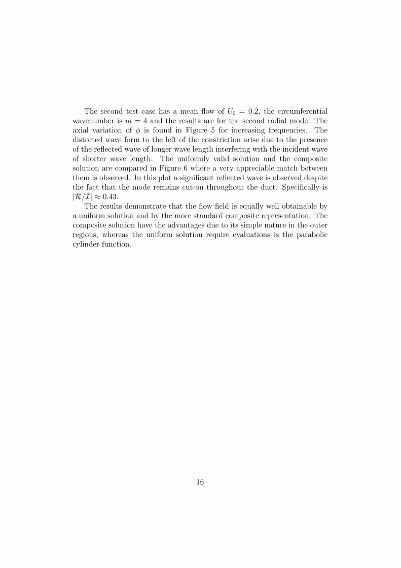
The second test case has a mean flow of U0 = 0.2, the circumferentialwavenumber is m = 4 and the results are for the second radial mode. Theaxial variation of φ is found in Figure 5 for increasing frequencies. Thedistorted wave form to the left of the constriction arise due to the presenceof the reflected wave of longer wave length interfering with the incident waveof shorter wave length. The uniformly valid solution and the compositesolution are compared in Figure 6 where a very appreciable match betweenthem is observed. In this plot a significant reflected wave is observed despitethe fact that the mode remains cut-on throughout the duct. Specifically is|R/I| ≈ 0.43.

The results demonstrate that the flow field is equally well obtainable bya uniform solution and by the more standard composite representation. Thecomposite solution have the advantages due to its simple nature in the outerregions, whereas the uniform solution require evaluations is the paraboliccylinder function.

16

Out[5]=

aL

-0.5 0.0 0.5

-3

-2

-1

0

1

2

3

X

Φ

Out[4]=

bL

-0.5 0.0 0.5

-3

-2

-1

0

1

2

3

X

Φ

Out[3]=

cL

-0.5 0.0 0.5

-3

-2

-1

0

1

2

3

X

Φ

Figure 5: Second test case: Axial variation of φ, solid lines: outer solution, dashed line:inner solution. a) at ω = 11.635 (Xt = ±0.18), b) at ω = 11.654 (Xt = ±0.015), c) atω = 11.66. (Xt = ±i0.10)

17

´

´

´

´

´

´

´

´

´

´

´´

´

´

´

´

´

´

´

´

´

´

´

´

´

´

´

´

´

´

´

´

´

´

´

´

´

´

´

´

´

´

´

´

´

´

´

´

´

´´

´

´

´

´´

´

´

´

´

-0.5 0.0 0.5

-3

-2

-1

0

1

2

3

X

Φ

Figure 6: Second test case: Comparison of composite and uniform solution, second testcase at ω = 11.66. Solid-Dashed curve: composite solution, crosses: Uniformly validsolution.

-0.5 0.0 0.5

0.0

0.2

0.4

0.6

0.8

X

r

Figure 7: Second test case: Contour map of upper half plane of |φ/max(φ)| at ω = 11.654.Contour levels at intervals of 0.1.

18

7. Conclusions

In this paper a cylindrical flow duct of slowly varying diameter has beenconsidered and the WKB method has been employed to determine the slowlyvarying acoustic modes. An analysis of waves tunnelling through a narrowregion of evanescent wave motion is conducted and the explicit dependenceof the reflection and transmission coefficients on the tunnelling parameter isobtained. The results agree with the well known ones for large tunnellingdistances, and for the tunnelling distance decreasing to zero. By use of thereflection and transmission coefficients the acoustic field is represented bya composite solution consisting of WKB solutions away from the tunnellingregion and by parabolic cylinder functions in the vicinity of the tunnelling re-gion. A uniformly valid solution is also derived which is valid at any locationin the duct. This solution uses parabolic cylinder functions in conjunctionwith coordinate stretching.

The effect of tunnelling is demonstrated at various frequencies for a zeromean flow test case and a test case with a mean flow. Through the test casesare a very accurate match between the composite and the uniform solutiondemonstrated. The test cases also show how an incident mode that remainspropagating throughout the duct causes a reflection from the constriction.

It seems natural to extend the results to include annular ducts whichwould allow the results to be directly applicable to study more realistic air-craft engine geometries similar to [11]. The results can furthermore serveas important reference solutions when numerical techniques, such as com-putational aero-acoustic codes, are employed to capture the details of wavespassing through a neck of a waveguide. The results generally enhance the op-tion to remain using multiple-scales methods to estimate the noise pollutionfrom aircraft engines and the relatively simple expression for reflection andtransmission coefficients should likewise help detecting if internal resonancesbuilds up.

Acknowledgement

The research is funded by The Danish Council for Independent Research,Technology and Production Sciences Grant number: UK 95 OS63822 PO83004.

19

References

[1] S. W. Rienstra, Sound transmission in slowly varying circular and annu-lar lined ducts with flow, Journal of Fluid Mechanics 380 (1999) 279–296,doi: 10.1017/S0022112098003607.

[2] S. W. Rienstra, Sound propagation in slowly varying lined flow ducts ofarbitrary cross-section, Journal of Fluid Mechanics 495 (2003) 157–173,doi: 10.1017/S0022112003006050.

[3] A. J. Cooper, N. Peake, Propagation of unsteady distubances in slowlyvarying duct with mean swirling flow, Journal of Fluid Mechanics 445(2001) 207–234, doi: 10.1017/S0022112001005559.

[4] E. Brambley, N. Peake, Sound transmission in strongly curved slowlyvarying cylindrical ducts with flow, Journal of Fluid Mechanics 596(2008) 387–412, doi: 10.1017/S0022112007009603.

[5] J. B. Keller, Uniform solutions for scattering by a potential barrier andbound states of a potential well, Am. J. Phys. 54 (6) (1986) 546–550,doi: 10.1119/1.14560.

[6] E. J. Hinch, Perturbation Methods, Cambridge University Press, 1991.

[7] C. M. Bender, S. A. Orszag, Advanced Mathematical Methods for Sci-entists and Engineers, McGraw-Hill, 1978.

[8] N. C. Ovenden, A uniformly valid multiple scales solution for cut-on cut-off transition of sound in flow ducts, Journal of Sound and Vibration 286(2005) 403–416, doi: 10.1016/j.jsv.2004.12.009.

[9] A. D. Pierce, Acoustics, an Introduction to its Physical Principles andApplications, McGraw-Hill, 1981.

[10] F. W. J. Olver, D. W. Lozier, R. F. Boisvert, C. W. Clark, NIST Hand-book of Mathematical Functions, Cambridge University Press, 2010.

[11] S. W. Rienstra, W. Eversman, A numerical comparison between themultiple-scales and finite-elelment solution for sound propagation inlined flow ducts, Journal of Fluid Mechanics 437 (2001) 367–384, doi:10.2514/6.1999-1821.

20

Paper 3

Nielsen R.B, Sorokin S.V. (under review): ”Periodicity effects of axial wavesin elastic compound rods” Journal of Sound and Vibration

69

PAPER 3

70

Periodicity effects of axial waves in elastic compound rods

R.B. Nielsen, S.V. Sorokin

Department of Mechanical and Manufacturing Engineering, Aalborg University,Fibigerstraede 16, 9220 Aalborg, Denmark

Abstract

Floquet analysis is applied to the Bernoulli-Euler model for axial waves ina periodic rod. Explicit asymptotic formulae for the stop band borders aregiven and the topology of the stop band pattern is explained. Eigenfrequen-cies of the symmetric unit cell are determined by the Phase-closure Principle,and their correspondence with stop band formation is shown. Steady-stateand transient dynamics of a periodic rod of finite length are analysed nu-merically and the difference in structural response when excitation is donein either stop- or pass bands is demonstrated. A physical interpretation ofthe underlying mechanisms of stop bands is proposed.

Keywords: Periodicity effects, Axial waves, Phase-closure Principle,Transient effects, Band gaps

1. Introduction

Analysis of wave propagation in periodic structures is a classical topicin theory of guided waves and has been studied for centuries. The classi-cal textbook on this topic is [1] which demonstrates the diversity of possiblerealms of physics in which the periodicity phenomenon is of interest. Acous-tic and electromagnetic (in particular, optical) waveguides have gained muchattention from this viewpoint [2], [3], [4], [5], and [6]. Periodicity effects aris-ing in the theory of elastodynamics and in vibroacoustics have been studiedin [7] and [8], surface waves in periodic plates in [9], and surface waves onperiodic elastic half spaces are for instance studied by [10] and [11].

A variety of methods has been employed in the abovementioned ref-erences. The choice of a method to analyse the problem depends upon

Email address: rn@m-tech.aau.dk (R.B. Nielsen)

Preprint submitted to Journal of Sound and Vibration April 6, 2015

whether a three-, two- or one-dimensional formulation is used. For analy-sis of three- and two-dimensional waveguides, the method of multiple scalesand Floquet’s theorem appear to be the preferred choices [2]-[6], althoughalternative methods, such as null field approach [12], have also been used.A common explanation of the band gap phenomenon is the so-called Braggresonance which originates from constructive interference of the multiplereflections occurring from the periodic perturbation of the waveguide, al-though an alternative non-Bragg resonance mechanism of generation of stopbands in two-dimensional waveguides has been discussed in [5].

In structural dynamics, a canonical and much studied model is an ide-alised lumped parameter system consisting of point masses and masslesssprings, see for instance [1]. Similarly, wave propagation in one- and two-dimensional lattices composed of masses and springs is treated in [13]. Con-tinuous one-dimensional structures such as beams with periodic supportshave been considered amongst others in [14] and [15]. Numerous papers areconcerned with analysis of more complex one-, two-, and three-dimensionalelastic structures such as fluid filled curved pipes [16], elastic plates withperiodic inclusions of rigid pins in [17], and elastic waves in a medium withperiodically spaced spheres in [18], where the dependence between impen-dence mismatch and existence of band gaps is also discussed. A rather exten-sive review of periodicity studies can be found in [19] encompassing variousstructures like beams, rib-skin structures, periodically stiffened cylinders,etc.

It is natural to conclude from the abovementioned references, that theperiodicity phenomenon may be employed for tailoring dynamic characteris-tics, such as insertion losses and eigenfrequencies, of non-uniform structures,as has been done, for example, in [20] and [21]. To guide such a tailoring,it is expedient to have simple formulae relating waveguide parameters toband gap locations and shapes. Despite the variety of areas and diversity ofspecific problems in wave propagation in periodic waveguides, not much at-tention has been given to pursue such formulae. The present paper is aimedto fill in this gap by means of rigorous asymptotic analysis of characteris-tic equations and consistent use of the Phase-closure Principle. To exercisethese tasks, a model, which is as simple as possible and as complicated asnecessary should be chosen.

The mass-spring structures, compared to the continuous structures, lackthe basic wave motion in the constituents which to the authors opinion isan essential ingredient in the understanding of stop and pass bands in con-tinuous structures. Continuous structures such as beams considered by [14],however, add further complexities which are not directly related to the ex-

2

istence of stop bands, more specifically evanescent and dispersive travellingwaves. For these reasons we choose to employ the Bernoulli-Euler model foraxial waves in rods which does allow wave motion in its basic constituents,but do not support evanescent and dispersive travelling waves. Fortunately,the Bernoulli-Euler model is the low frequency asymptotical reduction ofplane symmetric waves in an elastic layer, see [22]. The acoustic analogy tothis model is the somewhat unrealistic model for plane acoustic waves in aduct with a multi-component periodic gas. Such a periodic waveguide wasin fact also considered by [1] as a special case of problems governed by Hill’sequation, but this reference did not present results and provide physical in-terpretations similar to those given in this paper. A similar problem wasalso studied in [23], but here attention was given to topology optimisation ofa two material compound rod with the objective to maximise eigenfrequencygaps.

Our aim is to highlight the underlying mechanisms involved in the gen-eration of stop bands in a periodic Bernoulli-Euler rod. In Section 2 resultsfrom Floquet analysis and the reflection and transmission coefficients atan interface are provided. Already here an advantage of the model chosenarises since all waveguide properties are condensable to just two principleparameters both having a clear physical meaning. In Section 3 we providesome important details of the physics behind stop bands obtained throughasymptotic analysis of the results reported in Section 3. Section 4 discussesthe topology of the stop band pattern and its relation to the waveguide pa-rameters. In Section 5 the Phase-closure Principle is applied in order to linkresonance criteria for a unit cell and the individual segments to the locationof stop band borders and pass band locations. The results obtained so farare discussed in Section 6 where emphasis is put on physical interpreta-tion of the findings made throughout preceding Sections. Lastly, in Section7, steady-state forced response of a rod with periodic insert is consideredin two alternative formulations. The numerical analysis of transients in arod is also presented and energy accumulation/transmission is discussed.Conclusions are given in Section 8.

2. The model

The model employed is shown in Figure 1 where a unit cell from aninfinite structure is sketched. We initially define the unit cell as a rodconsisting of two segments whose uniaxial stress wave speeds are given bycj =

√Ej/ρj , where Ej is the elastic modulus and ρj is density. If the unit

cell is viewed as a strip cut from a plate, then the plane strain wave speeds

3

L1

L1/2L1/2

L2

L2

b)Segment 2

Segment 1 Segment 1

Segment 1Segment 2

xnxn-1 xn+1

x

Figure 1: Unit cell of present study consisting of segment 1 and segment 2. xn indicatesthe location of interfaces.

are cj =

√Ej

ρj(1−ν2j )

where νj are Poisson’s ratios. We designate lengths

and cross sectional areas as Lj and Aj (for a plate strip of height hj thenAj = 1 · hj , i.e. height per unit width) where the subscript j = 1, 2 denotethe segment number within the unit cell. The governing equation for axialwaves in non-dimensional form is:

∂2uj∂x2

− 1

c2j/c

21

∂2uj∂t2

= 0 (1)

where lengths have been scaled by L1, speeds by c1, and time by L1/c1. Iffurthermore, a non-dimensional frequency ω is introduced as ω = ΩL1/c1 ageneral solution to equation (1) is presented as:

uj(x, t) = αjeikjx−iωt + βje

−ikjx−iωt (2)

where kj = ωc1cj

is the non-dimensional wavenumber. The first term, the

α-term, represents a right going wave and the second term, the β-term,represents a left going wave. Consequently, α and β shall henceforth beused to designate right and left going waves.

2.1. Floquet analysis

The matching conditions and Floquet periodicity conditions are formu-lated, according to the unit cell shown in Figure 1, see also [1, Ch. 8]:

u1(1, t) = u2(1, t) (3a)

u′1(1, t) =E2A2

E1A1u′2(1, t) (3b)

u1(0, t) = u2(1 + L2/L1, t)λ (3c)

u′1(0, t) =E2A2

E1A1u′2(1 + L2/L1, t)λ (3d)

4

where primes denote derivatives wrt. x and the parameter λ is the propa-gation constant. The nontrivial solution to the above system of equationsexists when λ is a root of the characteristic equation:

λ2 + q(ω)λ+ 1 = 0 (4)

where:

q(ω) = −2 cos (ω) cos (τω) +

(1

κ+ κ

)sin (ω) sin (τω) (5)

in which τ = L2c2

c1L1

and κ = E2A2/c2E1A1/c1

= ρ2c2A2

ρ1c1A1have been introduced. The pa-

rameter τ can be interpreted as the ratio of propagation times. It is definedat the outset that τ ≤ 1, since any waveguide configuration where τ ≥ 1can be inverted to τ ≤ 1 simply by interchanging the segment numbering.The coefficient κ is the ratio of impedances of the two segments analog asthe acoustic impedance Z = ρc. We shall henceforth refer to κ as impedancemismatch parameter. Throughout the subsequent discussion the advantageof collecting all waveguide parameters in just the two quantities κ and τbecomes clear.

Inspection of the solution to the quadratic equation (4) reveals that|q(ω)| > 2 (when the discriminant is positive) leads to |λ| 6= 1 and thereforedefines a stop band. For an impedance matched rod, i.e. κ = 1, it isimmediately noticed that q(ω) will never be larger than two and stop bandswill therefore not be present.

3. Asymptotic analysis of stop band borders

The inequality |q(ω)| > 2 is what predicts the formation of stop bandsand this Section is devoted to gaining some understanding of this. We dothis by establishing asymptotic results of stop band borders for small andlarge impedance mismatches, respectively.

3.1. Small impedance mismatch asymptotic approximations

First, we conveniently notice that for an impedance matched unit cell(κ = 1) q(ω) simplifies to:

q(ω) = −2 cos(ω + τω) (6)

Thus |q(ω)| = 2 at the frequencies:

ωcrit =nπ

τ + 1(7)

5

which we throughout the paper refer to as critical frequencies. Suppose nowthe rod has a small impedance mismatch, say κ = 1+ε, then q(ω) breaks thebarrier |q(ω)| = 2 and a relatively narrow stop band is therefore generatedin the vicinity of the critical frequency. This suggests asymptotic analysisof equation (5) for small perturbations of perfectly matched impedance.

Let us first define that ε is a small positive parameter and take κ = 1+ε.Insertion of this in (5) and expanding leads to the relation

±2 ∼ −2 cos(ω) cos(τω) +(2 + ε2 − ε3 + ε4 +O(ε5)

)sin(ω) sin(τω) , ε→ 0

(8)

The frequency is now expanded in the usual way:

ω ∼ ω0 + εω1 + ε2ω2 + ε3ω3 +O(ε4) as ε→ 0 (9)

After inserting this in equation (8) and expanding the trigonometric func-tions for small ε, we compare terms of the same order, and find to leadingorder:

ε0 : ±2 = −2 cos((1 + τ)ω0) ⇒ ω0 =nπ

τ + 1(10)

which was known in advance. The O(ε) terms turn out to be identically zerowhen employing (10), but by balancing terms of O(ε2), O(ε3), and O(ε4) thefollowing is obtained:

ω1 = ±(τ + 1)−1

√√√√1

2− 1

2

cos(nπ 1−τ

1+τ

)

cos(nπ)(11)

ω2 =cos(ω0(1− τ))− cos(nπ) + (1− τ)ω1 sin(ω0(1− τ))

4(1 + τ2)ω1 cos(nπ)(12)

ω3 =[ (

6− 3(1 + τ)2ω21 + (1 + τ)4ω4

1 − 12(1 + τ)2ω22

)cos(nπ)+

3((τ − 1)2ω2

1 − 2)

cos((1− τ)ω0) + 6(τ − 1)(ω1 − ω2) sin((1 + τ)ω0)]

/(24(1 + τ)2ω1 cos(nπ)

)(13)

Further terms in the expansion (9) are trivial, but cumbersome and thereforenot presented here. The result is consequently two versions of (9), stemmingfrom the ± in (11), representing the left and right boundary of the stop

6

bands. The results are valid for any n each corresponding to a criticalfrequency from where a stop band develops.

The result of this analysis including up to O(ε3) terms in (9) is shownin Figure 2 along with the direct numerical results obtained from (5) forτ = 1/3. One may remark that for this value of τ it turns out that ω1 = 0when n = 4 which effectively corresponds to a stop band of zero width. Infact for integral values of 1/τ the n = 1/τ + 1 critical frequency has a zerowidth stop band.

5 10 15Ω

1.5

2.0

2.5

3.0

Κ

Figure 2: Borders of stop bands for n = 1, 2, 3, 5, 6, 7 for small impedance mismatch andτ = 1/3. Dotted curve: exact results, Dashed curve: asymptotic results.

We may interpret the critical frequencies as the ’seeds’ from where stopbands emerge when κ increases. This also means that the centre of a stopband will be found in the vicinity of nπ/(1 + τ), it can however be seenfrom Figure 2 that the stop bands at n = 1, 3, 5, 7 grow slightly asymmetricaround their critical frequencies. But the critical frequency will always becontained in the stop band.

3.2. Large impedance mismatch asymptotic approximations

Similar to the above analysis it is possible to obtain some approximationsfor stop band borders when κ is large. Specifically we prescribe that κ ∼ 1/εas ε → 0. Again we expand the frequency by ω ∼ ω0 + εω1 + ε2ω2 + O(ε3)as ε→ 0, and compare terms of same order. These yields:

O(ε−1) : sin(ω0) sin(τω0) = 0 ⇒ ω0,1 = nπ and ω0,2 = mπ/τ(14)

where n and m are integers. The leading order term ω0,2 = mπ/τ relates tothe location of zero width stop bands in Figure 2. The other leading orderterm ω0,1 are the locations of the pass bands that are not adjacent to a zero

7

width stop band. It shall be demonstrated later that a different expansionof the frequency is required for ω0 = ω0,2 when 1/τ is integral. For now weproceed as before and compare higher order terms and find:

O(1): ω1 =±2 + 2 cos(ω0) cos(τω0)

τ cos(τω0) sin(ω0) + cos(ω0) sin(τω0)(15)

O(ε): ω2 =−2τω1 cos(ω0)(ω1 cos(τω0) + 2 sin(τω0))

2τ cos(τω0) sin(ω0) + cos(ω0) sin(τω0)

+sin(ω0)

((1 + τ2)ω2

1 − 2)

sin(τω0)− 4ω1 cos(τω0)

τ cos(τω0) sin(ω0) + cos(ω0) sin(τω0)(16)

This approximation, including up to O(ε2) terms in ω, are compared to thedirect numerical results in Figure 3. A very appreciable correspondence isobserved between the two results. The above expressions for ω1 and ω2 areseen to fail when ω0 = ω0,2 and 1/τ is integral due to division by zero. Thecause of the failure is seen from (14) where ω0 = ω0,2 turns out to be a doubleroot. The encounter of double roots is often a sign of a challenging problem[24]. To overcome this difficulty we suggest an alternative expansion of ω:

ω ∼ ω0,2 + ε1/2ω1 + εω2 + ε3/2ω3 +O(ε2)

as ε→ 0 (17)

Again by expanding the equation for q(ω) and compare terms of equal orderdo we find:

O(ε−1/2) :0 (18)

O(ε0): ω1 = ±√±2 + cos(ω0,2) cos(τω0,2)

τ cos(ω0,2) cos(τω0,2)(19)

O(ε1/2): ω2 = 0 (20)

O(ε1): ω3 =(1 + τ2)ω1(τω2

1 − 6)

12τ(21)

These are valid only when 1/τ is integral. The result is compared to thedirect numerical solution in Figure 4 where terms of O(ε3/2) is included.Again, a very appreciable match is observed between the asymptotic ap-proximations and the direct numerical solution.

In case the parameter 1/τ is non-integral the stop band borders are allcaptured by the results in (14)-(16). Some of them, however, diverges fromthe correct result even for relatively large values of κ. This is illustrated in

8

Figure 5 where 1/τ = 1/3.3 is taken. Values of n and m corresponding toeach leading order term in (14) are indicated as well. The left most stopband in the Figure have both m = n = 0 and ω0 is therefore again a doubleroot of (14) and this stop band border is therefore approximated by (17).

5 10 15 20Ω0

5

10

15

20Κ

Figure 3: Borders of stop bands for n = 1, 2, 4, 5 for large impedance mismatch andτ = 1/3. Dotted curve: exact results, Dashed curve: asymptotic results.

5 10 15Ω

5

10

15

20

Κ

Figure 4: Borders of stop bands for m = 0, 1, 2 for large impedance mismatch and τ = 1/3.Dotted curve: exact results, Dashed curve: asymptotic results.

We shall return to a more physical interpretation of the asymptotic for-mulae in Section 6.

4. Topology of stop band pattern

In this Section the topology of the stop band pattern is discussed. Thesolid and dashed lines in the subsequent plots correspond to the two rootsof (4).

9

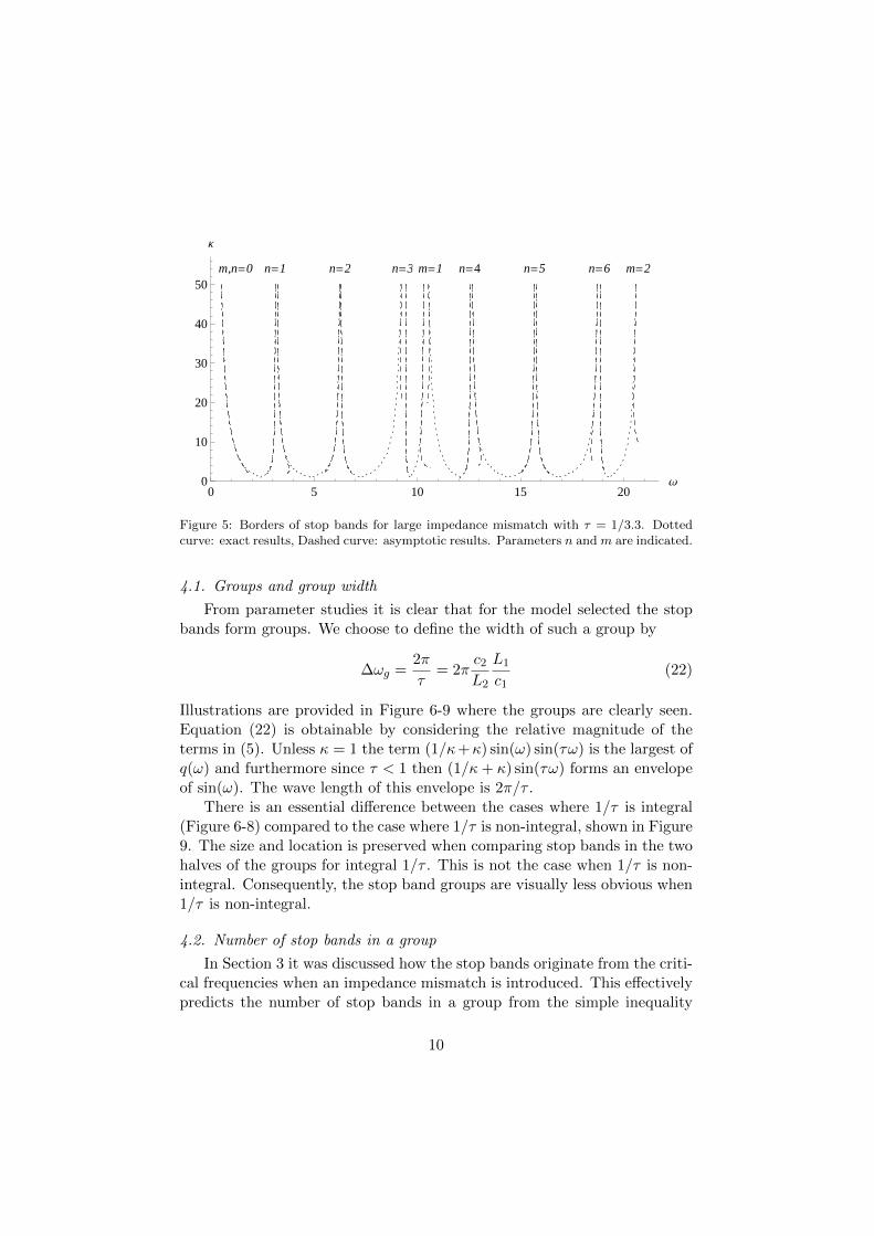
0 5 10 15 20Ω0

10

20

30

40

50

Κ

n=1 n=2 n=3 n=4 n=5 n=6m,n=0 m=1 m=2

Figure 5: Borders of stop bands for large impedance mismatch with τ = 1/3.3. Dottedcurve: exact results, Dashed curve: asymptotic results. Parameters n and m are indicated.

4.1. Groups and group width

From parameter studies it is clear that for the model selected the stopbands form groups. We choose to define the width of such a group by

∆ωg =2π

τ= 2π

c2

L2

L1

c1(22)

Illustrations are provided in Figure 6-9 where the groups are clearly seen.Equation (22) is obtainable by considering the relative magnitude of theterms in (5). Unless κ = 1 the term (1/κ+κ) sin(ω) sin(τω) is the largest ofq(ω) and furthermore since τ < 1 then (1/κ+ κ) sin(τω) forms an envelopeof sin(ω). The wave length of this envelope is 2π/τ .

There is an essential difference between the cases where 1/τ is integral(Figure 6-8) compared to the case where 1/τ is non-integral, shown in Figure9. The size and location is preserved when comparing stop bands in the twohalves of the groups for integral 1/τ . This is not the case when 1/τ is non-integral. Consequently, the stop band groups are visually less obvious when1/τ is non-integral.

4.2. Number of stop bands in a group

In Section 3 it was discussed how the stop bands originate from the criti-cal frequencies when an impedance mismatch is introduced. This effectivelypredicts the number of stop bands in a group from the simple inequality

10

5 10 15Ω

0.5

1.0

1.5

2.0

2.5

3.0

Λ¤

Figure 6: Stop band pattern with τ = 1/3and κ = 1/3. ∆ωg = 6π. Vertical gridlines at 3π and 6π.

5 10 15 20 25 30 35Ω

0.5

1.0

1.5

2.0

2.5

3.0 Λ¤

Figure 7: Stop band pattern with τ = 1/6and κ = 1/3. ∆ωg = 12π. Vertical gridlines at 6π and 12π.

5 10 15 20 25Ω

1

2

3

Λ¤

Figure 8: Stop band pattern with τ = 1/4and κ = 1/4. ∆ωg = 8π. Vertical gridlines at 4π and 8π.

5 10 15 20Ω

0.5

1.0

1.5

2.0

2.5

3.0

Λ¤

Figure 9: Stop band pattern with τ =1/3.2 and κ = 1/3.2. ∆ωg ≈ 20.1. Ver-tical grid lines at π/τ and 2π/τ .

ωcrit < ∆ωg. Thus, the number of stop bands in a group is the largest nsatisfying:

n < 2(

1τ + 1

)(23)

We know furthermore that these are found in the vicinity of the criticalfrequencies predicted by (7). It was ascertained earlier that some stop bandsdisappear when 1/τ is integral. In this case the formula for the number ofstop bands is:

n =2

τ(24)

11

5. Eigenfrequencies and Phase-closure Principle for periodic rods

Several papers have demonstrated the close relation between stop bandborders and the eigenfrequencies of a single unit cell provided this is sym-metric, see Figure 10. This matter is, for instance, discussed in [14] and [15],the former described the complicated wave motion in a beam with periodicsupports, and the latter derived eigenfrequency formulae for the same struc-ture incorporating the propagation constant. Considerations along theselines are expedient in the discussions of the topics in this paper. The rela-

L1

L1/2L1/2

L2

L2

Segment 2Seg. 1 Seg. 1

Segment 1Segment 2

xnxn-1 xn+1

x

Figure 10: Symmetric configuration of unit cell.

tion between eigenfrequencies and the Floquet plot becomes apparent whencomparing the discriminant of equation (4) to the eigenfrequency equationsfor the symmetric unit cell with free-free and fixed-fixed boundary condi-tions. By designating these eigenfrequency equations ffree(ω) and ffixed(ω),it turns out that the following relation holds:

q2(ω)− 4 =−1

16κ2ffree(ω)ffixed(ω) (25)

More details may be found in AppendixA. So the relation between eigen-frequencies and stop bands observed by [14] is therefore also present for thecurrent model.

5.1. Determination of critical frequencies by phase-closure principle

An attractive method for determining eigenfrequencies of a unit cell isthe phase-closure principle, as this likely leads to an important insight inthe physics at the transition from stop to pass band. Before doing so, weshortly discuss the applicability of the method to the problem at hand. Itis clear that the actual wave motion of a unit cell cannot be seen as a singleharmonic due to the difference in wave speeds. Thus, the motion will eitherhave to be interpreted as a superposition of a number of harmonics valid forall x, this view was adopted in [14]. Or alternatively, the wave motion can berendered as consisting of piecewise harmonic waves pertaining to a certainsegment. In the first case, it is not immediately obvious how the total phase

12

of the waves should be defined, but in the latter interpretation the notion ofphase change over a segment is quite obvious. Consequently the total phasechange can be established by summation of phase changes in each segment.In the following utilisation of the phase-closure principle we adopt the latterview of piecewise harmonic waves to construct the actual wave motion in aunit cell and shall refer to such a wave as a compound wave. In AppendixBwe show the Fourier content of an eigenmode as a complementary view ofhow the wave motion is interpreted in this Section.

The phase-closure principle states that when the total phase change awave experiences after completing a full circuit in a rod equals a multipleof 2π resonance occurs (see [25]). A simple way of stating the total phasechange for, say, a free-free rod is 2K1L1 + 2K2L2 where Kj = kj

c1L1

is thedimensional wave number. This implicitly assumes an impedance matchbetween the segments since any internal reflections at interfaces are ignored.Thus, the result must be expected to relate to the critical frequencies. Theresonance condition in non-dimensional form therefore becomes:

2ω

(L1c1

c1L1+L2c1

c2L1

)= 2πn ⇒ (26)

ω =nπ

1 + τ(27)

So this way of stating the resonance condition of a unit cell leads to thecritical frequencies and this is indeed an interesting result since it pointsout a simple way of determining where the stop bands appear. This alsoprovides some understanding of the critical frequencies. From equation (26)we understand that the critical frequencies are those where n half compoundwaves fits into a unit cell and, therefore, there is a πn phase change aftertraversing the unit cell once. So basically the critical frequencies is theeigenfrequencies of a compound wave when κ = 1. This is basically theBragg resonance condition, but with the wavelength defined with referenceto the compound wave. Thus, the stop bands arise around the frequencieswhere reflections of waves are in phase and therefore will interference.

5.2. Determination of stop band borders by phase-closure principle

The concept behind the phase-closure principle can be used, however,in a slightly different way where account is taken of internal reflections. Todo so we apply the systems of equations from AppendixA representing thefree-free and fixed-fixed rods and remove the boundary equation concerningthe left hand end of the rod. This results in two systems of five equationsin the six unknowns α1,2,3 and β1,2,3. When the reflected wave β1 returns

13

back perfectly in phase with the incident wave α1 (with the proper accountof a possible phase change at the left edge of the rod) resonance occurs. Theresult for a free boundary condition is conveniently stated in terms of theparameters κ and τ :

(β1

α1

)

free

=eiω(1− κ2 − eiω(−1 + κ)2 + ei(1+2τ)ω(1 + κ)2 + e2iτω

(−1 + κ2

))

(1 + κ)2 + eiω (−1 + κ2)− e2iτω(−1 + κ) (−1 + κ+ eiω(1 + κ))

(28)

A similar result for a fixed boundary condition can be determined as well.The quantities φfree = phase(β1/α1)free and φfixed = phase(β1/α1)fixed−π (toaccount for the phase shift at the left boundary of the unit cell) are plottedin Figure 11 and 12. This enables the simple reading of eigenfrequenciesbeing the locations where the curves pass the abscissa. One can remark inthe latter Figure that the curves are lie on top of each other.

5 10 15Ω

-3

-2

-1

1

2

3

Φfree,Φfixed

Figure 11: Solid line: φfree, Dashed Line:φfixed. κ = τ = 1/3. Grid line is lo-cated at 3π. Stop bands are shown in thebackground. Eigenfrequencies are locatedwhere the curves crosses zero.

5 10 15Ω

-3

-2

-1

1

2

3

Φfree,Φfixed

Figure 12: Solid line: φfree, Dashed Line:φfixed. κ = 1 and τ = 1/3. Grid line islocated at 3π.

A skew symmetric behaviour is apparent from Figure 11 in the followingway: a stop band in the first half of the group, i.e. below ω = π/τ = 3π,having a free-free eigenfrequency on its left border has a similar stop band inthe upper half of the group, but with a free-free eigenfrequency on its rightboundary - and vice versa. In fact what happens is that eigenfrequenciesmerge at ω = π/τ , as earlier mentioned, swap places between π/τ -2π/τ com-pared with 0-π/τ , merge and swap back when crossing 2π/τ . This patternrepeats itself for each multiple of 2π/τ . The quantities φfree and φfixed of theimpedance matched rod (Figure 12) are seen to be linear with frequency,and the eigenfrequencies are therefore evenly spaced and are predictable byformula (27).

14

6. Interpretation of results

As stated in Subsection 2.1 the origin of a stop band is due to animpedance mismatch between the segments and the width of the stop bandincreases with increasing impedance mismatch which was demonstrated inSection 3, see equation (5).

The results from the asymptotic analysis of small impedance mismatchhint at some finer details of the physics involved in the stop band creation.By means of the first two terms in the expansion of ω scaled to dimensionalfrequency we find stop bands in the intervals Ω1 < Ω < Ω2 where

Ω1,2 = Ωcrit

(1± (κ− 1)

√1

2− 1

2

cos (Ωcrit∆t)

cos(ΩcritT )+O((κ− 1)2)

)(29)

in which we have introduce T = L1/c1 + L2/c2, the time for a disturbanceto traverse a unit cell, and ∆t = L1/c1 − L2/c2 being the difference inpropagation time in the two segments. The parameter ∆t has the followingphysical significance: From a scattering process at the interface at xn, seeFigure 1, one wave will travel towards the xn−1 interface, reflect again andtravel back towards xn. Meanwhile will a wave travel from xn to xn+1 andreflect back to xn. In general there will be a time delay between arrivalback to the xn interface and ∆t is exactly half this time delay or simply thetime difference between arrival of the left and right going wave to the xn−1

and xn+1 interfaces, respectively. So we may interpret the quantity Ωcrit∆tas a ’phase loss’ due to the time delay between waves reflecting back to aninterface. So, what drives the creation of a stop band is the mismatch ofimpedances, κ− 1 6= 0, alongside with this phase loss. With this in mind itis not difficult to imagine what happens physically in the case of zero widthstop bands as discussed in Section 3. Since the phase loss grows with n thephase loss may add up to a complete circuit and no stop band is created.

From the large impedance mismatch asymptotic results we also get ahint of why the pass bands are maintained as κ→∞. As κ grows the widthof the pass bands decreases like 2/κ and becomes just ’pass points’ (ratherthan pass bands) in the limit, and are located at ω0,1 = nπ and ω0,2 = mπ

τ .By scaling these to dimensional quantities we find:

Ω0,1 = nπc1

L1(30)

Ω0,2 = mπc2

L2(31)

15

It is rapidly obtained that these are the eigenfrequencies, with boundarieseither free or fixed, of segment 1 and segment 2, respectively. So when theimpedance mismatch is large the relatively narrow pass bands appear aroundthe eigenfrequencies of the individual segments. Opposite the interpretationof critical frequencies may we interpret the eigenfrequencies of the individualsegments as the seeds from where a pass band emerges when κ decreasesfrom infinity. This furthermore points out the reason for creation of groupsas explained in Section 4. These are formed by the eigenfrequencies ofthe segment with the fastest propagation time, and the stop bands in sucha group are hence constrained between the eigenfrequencies of the othersegment.

It is expedient to discuss the reflection and transmission process at aninterface in the case of a large impedance mismatch. Generally will a wavedesignated α1 which is incident on an interface reflect a wave with amplitudeβ1 = −κ−1

κ+1α1 and transmit a wave of amplitude α2 = (1 − κ−1κ+1)α1. In the

case when κ >> 1 a wave propagating in segment 1 will be almost fullyreflected, i.e. β1/α1 ≈ −1, when it is incident on the interface to segment2. Consequently, the transmitted wave will be very small, α2/α1 ≈ 0. I.e.the result basically corresponds to a fixed boundary condition. Explainedin words, a wave becomes trapped in the small, compliant, and fast segmentas it propagates back and forth and keeps being reflected when it meets thelarge, stiff, and slow segment.

From the above discussions we now know that it is a trivial matter toapply the phase-closure principle to determine:

• Locations of stop bands for small impedance mismatches as the criticalfrequencies.

• Locations of pass bands for large impedance mismatches as the eigen-frequencies of the individual segments.

• Borders of stop bands for any value of κ as the eigenfrequencies of thesymmetric unit cell.

So the creation of stop and pass bands as explained above all correspond tocreation of resonances of either the compound structure or the individualsegments. As a final comment it is argued that higher stop band groups arejust higher harmonic versions of the lowest stop band group. The reasoningbehind this statement is that the stop bands are bounded by eigenfrequencieswhere the successive occurrences of these are higher harmonic phenomenacompared to the first.

16

7. Steady-state and transient forced response of a rod with theperiodic insert

The analysis reported in the previous Sections has been restrained tosteady-state free waves in an infinitely long periodic waveguide. For anyapplication, however, it is necessary to account for the finite length of aperiodic segment, to specify its loading conditions, and to consider transientsin its performance. These issues are tackled in this Section.

The attenuation levels predicted for the stop bands by means of theFloquet theory are known to be in an excellent agreement with the inser-tion losses for structures containing a few periodicity cells [26]. The insertionlosses are commonly estimated as the ratio of the power flow into a structurewithout and with the periodic segment, IL = 10 log(P0/Pn). This formula-tion implies that the same force is applied at the same place and the samefrequency on a structure with/without the insert and only the steady-stateresponse is accounted for. Such a concept differs from the idea of solvingthe equation (4) to determine propagation constants for free waves. Theseconstants, by definition, specify the ratio between the complex-valued axialdisplacements at two arbitrary cross-sections in a periodic rod provided thatthe distance between them equals the length of a periodicity cell. No forcingis involved in this definition.

Therefore, it is of interest to derive a transfer matrix for free incidentwaves of unit amplitude traversing an array of a finite number of periodicitycells, extended further out as a homogeneous rod, and to compare to thepropagation constants for an infinite periodic structure. For consistency,the comparison should be extended to the stationary forcing problem forthe same layout of a rod with the periodic insert. The transfer function inthis case is derived as the complex-valued amplitude of the outgoing wavedriven by a force of the unit amplitude at the inlet.

The derivation of transfer matrices is a straightforward matter, and theend results are illustrated in Figure 13 for the insert consisting of two pe-riodicity cells. The parameters of these cells are the same as those used toin Figure 6. The complex-valued amplitudes of outgoing waves have beenobtained in the closed analytical form by means of symbolic manipulatorMathematica, but the formulae are rather cumbersome, and, therefore, notpresented here. The same holds true for the propagation constants foundfrom equation (4), squared to account for traversing two periodicity cells.These constants are dependent only upon κ and τ , whereas their counter-parts found from transfer matrices feature dependence upon κ, L2/L1 andc1/c2. However, the shapes of curves obtained for different L2/L1 and c1/c2

17

with τ being preserved are almost the same in the stop bands regions.

5 10 15Ω

2

4

6

8

Λ¤

Figure 13: Solid lines: The Floquet propagation constants found for an insert consisting oftwo periodicity cells, Dashed lines: the transfer function from the forcing problem, Dottedlines: the transfer function for an incident wave of unit amplitude.

As seen from Figure 13, the solution of the forcing problem for just twoperiodicity cells agrees with predictions of the Floquet theory much betterthan the solution of the ’incident wave’ problem. This result suggests that anassumption of the perfect source, employed in the forcing problem, mimicsthe interaction pattern of free waves in an infinite periodic structure quiteaccurate. The analysis of a structure of the transfer matrix of a single unitcell inserted in an infinite homogeneous waveguide lies beyond the scope ofthis paper.

Though substantial effort has been given to analysis of stationary wavemotion in periodic structures, much less efforts have been made to studytransient effects in such structures. The remaining part of this Sectionis devoted to such a study. As seen from Figure 13, the solution of thesteady-state forcing problem agrees fairly well with results obtained for aninfinite periodic structure. Therefore, it is reasonable to expect that thetransients observed in solving the forcing problem in time domain with initialconditions represent their counterpart in an infinite periodic structure.

The Newmark integration scheme has been implemented in a finite el-ement (FE) code with Newmark parameters γ = 1/2 and β = 1/4. The

18

element length is chosen so there are at least 10 elements per wave length,and the size of the time step is based on a Courant number of 1/5. Themodel, which is shown in Figure 14, is made with 6 symmetric unit cells con-nected to a semi-infinite rod in the right hand end modelled as an impedanceboundary condition tuned to give no reflection when a wave is incident onit. The structure is excited at the left end by a harmonic force. All parame-ters are taken as unity, but with c2 = 3m/s corresponding to the stop bandpattern in Figure 6. The excitation force is defined as P (t) = cos(Ωt).

P(t)∞

Figure 14: Periodic waveguide applied in the transient model.

To illustrate the wave attenuation from excitation in a stop band weprovide in Figure 15 a plot of deflections determined from the FE code andthe corresponding Floquet modes, determined from (3). The axial deflec-tions are shown on the vertical axis and scaled with the deflections at x = 0.There is an appreciable similarity between the transient FE result and theFloquet mode in Figure 15 despite the fact that the Floquet mode assumesan infinite periodic structure and the FE results only includes six unit cells.The attenuation effect is also seen to arise even with a fairly small num-ber of periodicity cells and already after traversing three unit cells is theattenuation significant.

0 2 4 6 8 10 12−2

−1

0

1

x

u

Figure 15: Deflections at Ω = 4.5046rad/s (a stop band) at t = 250s. Dots: segment 1,Crosses: segment 2, Solid line: deflections determined from Floquet analysis. SI units areused.

It is of interest to trace the work done by the excitation force, the energyflowing out of the structure, and thereby also the energy accumulated inthe structure. This is done exactly at an eigenfrequency and in its near

19

proximity. Specifically, the eigenfrequency Ωn = 5.5046rad/s correspondingto a stop band border as seen in Figure 6, is selected. The results areprovided in the Figures 16-18. As a first observation it is noticed thatthe solution becomes stationary which is achieved when the accumulatedenergy, the crosses, becomes constant. The largest amount of energy canbe injected into the structure when excited at the eigenfrequency whichleads to the largest energy accumulation. It seems intuitive that when theexcitation is in the pass band more energy can leak out of the non-reflectingboundary condition since waves can now propagate through the structure.As a consequence hereof is the amount of accumulated energy smaller inFigure 18 compared to 17.

The underlying mechanism of the small energy injection when excitationis in a stop band, Figure 16, becomes clear when tracing the phase shifthistory between the velocity of the first node and the excitation force. Theseare given in Figure 19 and 20. Apparently the phase shift closes in on −π/2and the excitation force can therefore not inject energy into the structure.One remarks that the power injection is:

Pin =1

2PV1 cos(θ) (32)

where θ is the phase angle between the excitation force P and nodal velocityV1. So at phase shifts in the vicinity of ±π/2 only very little power can beinjected.

8. Conclusions

In this paper axial waves in a periodic Bernoulli-Euler rod have beenanalysed in order to facilitate the understanding of periodicity effects andstop bands. This has been done by Floquet analysis, asymptotic analysis,and by the phase-closure principle.

Two principle parameters, namely, the impedance mismatch and the ra-tio of propagation times, are introduced, and the relation of the stop bandpattern with these parameters is explained and quantified. It is found, byapplication of the phase-closure principle, that the stop band locations arelinked to the eigenfrequencies of an impedance matched symmetrical unit cellwith symmetrical boundary conditions. It is also found that pass bands arealways located at the eigenfrequencies of the individual segments with sym-metrical boundary conditions regardless of the impedance mismatch. The

20

0 500 1000 1500 20000

5

10

Time

Ene

rgy

Figure 16: Energies when excited inside the stop band (at Ω = (5.5046−0.1)rad/s). Dots:Energy in, Crosses: Energy accumulated, Solid line: Energy out. SI units are used.

0 500 1000 1500 20000

500

1000

Time

Ene

rgy

Figure 17: Energies when excited exactly at an eigenfrequency (at Ω = 5.5046rad/s).Symbols are the same as in Figure 16.

0 500 1000 1500 20000

500

1000

Time

Ene

rgy

Figure 18: Energies when excited inside the pass band (at Ω = (5.5046 + 0.1)rad/s).Symbols are the same as in Figure 16.

21

0 1000 2000−0.4

−0.3

−0.2

−0.1

0

Time

Pha

se s

hift

[π]

Figure 19: Phase shift between velocityof first node and excitation force at Ω =(5.5046 + 0.1)rad/s (pass band).

0 1000 2000

−0.5

−0.4

−0.3

−0.2

−0.1

0

TimeP

hase

shi

ft [π]

Figure 20: Phase shift between velocityof first node and excitation force at Ω =(5.5046 − 0.1)rad/s (stop band).

exact location of stop band borders is determined numerically by the phase-closure principle applied in an untraditional manner, and simple asymptoticformulae for small and large impedance mismatch are derived.

The steady-state forcing problem for a rod with a periodic insert is solvedin two formulations, and results are shown to be in agreement with Floquetanalysis for an infinite rod. By transient FE analysis of harmonic forcingof a rod with the periodic insert it has been demonstrated that there is asignificantly smaller energy injection into the structure when it is excited ina stop band compared to in a pass band. The reason for this is shown tobe a −π/2 phase shift between excitation force and velocity response of thestructure at the excitation point.

The relations given relating τ to the topology of stop band patternbacked up with the formulae from the asymptotic analysis points out asimple way of choosing the unit cell parameters to have stop bands wheredesired. Since only few unit cells are needed to have an appreciable waveattenuation, it is reasonable to suggest that broad band mechanical filterscan be designed by combining different unit cells with overlapping stop bandpatterns. Such a design is achievable from the simple formulae presented inthis paper.

22

Acknowledgement

The Research is funded by The Danish Council for Independent Re-search, Technology and Production Sciences Grant number: UK 95 OS63822PO83004.

AppendixA. Derivation of eigenfrequency equations

Here we derive the frequency equations for the symmetric unit cell withfree-free and fixed-fixed boundary conditions, and prove its relation to theFloquet discriminant. Referring to Figure 10 the matching equations at theinterfaces are setup as

u1(1/2) = u2(1/2) (A.1)

u′1(1/2) =E2A2

E1A1u′2(1/2) (A.2)

u2(1 + L2/L1) = u3(1 + L2/L1) (A.3)

E2A2

E1A1u′2(1 + L2/L1) = u′3(1 + L2/L1) (A.4)

valid regardless of boundary condition. The boundary conditions are simply:

free-free: u′1(0) = 0 u′3(

1 + L2L1

)= 0 (A.5)

fixed-fixed: u1(0) = 0 u3

(1 + L2

L1

)= 0 (A.6)

From here two systems of equations are setup and the frequency equationsare then found as the nontrivial solutions of these. Specifically they read:

ffree = −4i(2κ cos(τω) sin(ω) +

(−1 + κ2 +

(1 + κ2

)cos(ω)

)sin(τω)

)

(A.7)

ffixed = 4i(2κ cos(τω) sin(ω) +

(1− κ2 +

(1 + κ2

)cos(ω)

)sin(τω)

)(A.8)

The relation to stop bands may now be identified from the fact that:

q(ω)2 − 4

ffreeffixed=−1

16κ2(A.9)

which is frequency independent and therefore do the two transcendentalequations q(ω)2 − 4 and ffreeffixed share the same roots.

23

AppendixB. Fourier Decomposition

The analysis throughout the paper strongly implies that the complicatedeigenfrequency spectrum in a unit cell arises due to the reflections happeningat the interfaces between the segments. So, as earlier mentioned the resultingwave motion may be interpreted as a superposition of a large number ofwaves. This may be quantified by a Fourier decomposition on the modeshape. Such an analysis leads to the results in Figure B.21 where the first10 Fourier coefficients are plotted for each wave number for the unit cellconfiguration in Figure 6. We choose to do this at the eigenfrequency locatedat ωn ≈ 5.47. The mode shape, which is seen in Figure B.22, is symmetricabout x = (1 + L2/L1)/2 and consequently is it necessary to extract onlythe cosine coefficients. The spatial frequency content now becomes clear.

0 5 10 15 20 25 30

n Π

1+L2L1

2

-2.0

-1.5

-1.0

-0.5

0.5

an

Figure B.21: Fourier cosine coefficient (an) at eigenfrequency ωn = 5.47 for free-free rod.

0.5 1.0 1.5 2.0x

-3

-2

-1

1

2u

Figure B.22: Mode shape of free-free rod at ωn = 5.47

Firstly we notice that, as expected, the Fourier coefficients approach zero

24

rapidly as the wavenumber increases. The two actual wavenumbers at thisfrequency in the individual segments are k1 = 5.47 and k2 = 1.82 whichis recognisable from the plot since the largest Fourier coefficients are foundaround these wavenumbers.

References

[1] L. Brillouin, Wave propagation in periodic structures, Dover Publica-tions, 1946.

[2] O. R. Asfar, A. H. Nayfeh, The application of the method of multiplescales to wave propagation in periodic structures, Society for Industrialand Applied Mathematics 25 (1983) 455–480.

[3] Z.-Y. Tao, W.-Y. He, X. Wang, Resonance-induced band gaps in aperiodic waveguide, Journal of Sound and Vibrations 313 (2008) 830–840. doi:10.1016/j.jsv.2007.11.055.

[4] Z. Tao, W. He, Y. Xiao, W. Zhang, X. Wang, Sound transmissionwithin the bragg gap via the high-order modes in a waveguide withperiodically corrugated walls, Journal of Applied Physics 105 (2009)830–840. doi:10.1016/j.jsv.2007.11.055.

[5] V. A. Pogrebnyak, Non-bragg reflections in a periodicwaveguide, Optics Communications 232 (2004) 201–207.doi:10.1016/j.optcom.2003.12.067.

[6] C. Elachi, Acoustic microwave generation in a periodic piezoelectricmedium with drifting charges, Applied Physics 5 (1974) 159–164.

[7] P. Langlet, A.-C. Haldky-Hennion, J.-N. Decarpigny, Analysis of thepropagation of plane acoustic waves in passive periodic materials usingthe finite element method, J. Acoust. Soc. Am. 98 (1995) 2792–2800.doi:10.1121/1.413244.

[8] C. G. Poulton, A. B. Movchan, R. C. McPhedran, N. A. Nicorivici,Y. Antipov, Eigenvalue problems for doubly periodic structures andphononic band gaps, Proc. R. Soc. Lond. A. 456 (2000) 2543–2559.doi:10.1098/rspa.2000.0624.

[9] A. El-Bahrawy, Stopbands and passbands for symmetric rayleigh-lambmodes in a plate with corrugated surface, Journal of Sound and Vibra-tion 170 (1994) 145–160.

25

[10] S. Seshadri, Effect of periodic surface corrugation in the propagation ofrayleigh waves, J. Acoust. Soc. Am. 65 (1978) 687–694.

[11] A. Bostrom, Surface waves on the periodic boundary of an elas-tic half space, Applied Scientific Research 39 (1982) 129–142.doi:10.1007/BF00457015.

[12] A. Bostrom, Acoustic waves in a cylindrical duct with periodicallyvarying cross section, Wave Motion 5 (1983) 59–67. doi:10.1016/0165-2125(83)90007-0.

[13] J. S. Jensen, Phononic band gaps and vibrations in one- and two-dimensional mass-spring structures, Journal of Sound and Vibration266 (2003) 1053–1078. doi:10.1016/S0022-460X(02)01629-2.

[14] D. J. Mead, Free wave propagation in periodically supported, in-finite beams, Journal of Sound and Vibration 11 (1970) 181–197.doi:10.1016/S0022-460X(70)80062-1.

[15] G. S. Gupta, Natural flexural waves and the normal modes ofperiodically-supported beams and plates, Journal of Sound and Vibra-tion 13 (1970) 89–101. doi:10.1016/S0022-460X(70)80082-7.

[16] A. Søe-Knudsen, S. Sorokin, Modelling of linear wave propagationin spatial fluid filled pipe systems consisting of elastic curved andstraight elements, Journal of Sound and Vibration 329 (2010) 5116–5146. doi:10.1016/j.jsv.2010.06.015.

[17] S. G. Haslinger, N. V. Movchan, A. B. Movchan, R. C. McPhe-dran, Transmission, trapping and filterring of waves in periodicallyconstrained elastic plates, Proc. R. Soc. Lond. A. 468 (2012) 76–93.doi:10.1098/rspa.2011.0318.

[18] M. M. Sigalas, E. N. Economou, Elastic and acoustic wave bandstructure, Journal of Sound and Vibration 158 (1992) 377–382.doi:10.1016/0022-460X(92)90059-7.

[19] D. J. Mead, Wave propagation in continuous periodic structures: Re-search contributions from southampton, 1964-1995, Journal of Soundand Vibration 190 (1996) 495–524. doi:10.1006/jsvi.1996.0076.

[20] N. Olhoff, B. Nui, G. Cheng, Optimum design of band-gap beam struc-tures, International Journal of Solids and Structures 49 (2012) 3158–3169. doi:10.1016/j.ijsolstr.2012.06.014.

26

[21] A. Søe-Knudsen, Design of stop-band filter by use of curved pipe seg-ments and shape optimization, Struct Multidisc Optim 44 (2011) 863–874. doi:10.1007/s00158-011-0691-2.

[22] R. D. Mindlin, An Introduction to the Mathematical Theory of Vibra-tions of Elastic Plates, World Scientific, 2006.

[23] J. S. Jensen, N. L. Pedersen, On maximal eigenfrequency separation intwo-material structures: the 1d and 2d scalar cases, Journal of Soundand Vibration 289 (2006) 967–986. doi:10.1016/j.jsv.2005.03.028.

[24] E. J. Hinch, Perturbation Methods, Cambridge University Press, 1991.

[25] D. J. Mead, Waves and modes in finite beams: Application of the phase-closure principle, Journal of Sound and Vibration 171 (1994) 695–702.doi:10.1006/jsvi.1994.1150.

[26] A. Søe-Knudsen, S. Sorokin, R. Darula, Theoretical and experimentalanalysis of the stop-band behaviour of elastic springs with periodicallydiscontinuous curvature, J. Acoust. Soc. Am. 132 (2012) 1378–1383.doi:10.1121/1.4740480.

27