Embed Size (px)
Citation preview
Aalborg Universitet
Lifetime Investigation of PEM Electrolyzers under Realistic Load Profiles
Frensch, Steffen Henrik
Publication date:2018
Document VersionPublisher's PDF, also known as Version of record
Link to publication from Aalborg University
Citation for published version (APA):Frensch, S. H. (2018). Lifetime Investigation of PEM Electrolyzers under Realistic Load Profiles. AalborgUniversitetsforlag. Ph.d.-serien for Det Ingeniør- og Naturvidenskabelige Fakultet, Aalborg Universitet
General rightsCopyright and moral rights for the publications made accessible in the public portal are retained by the authors and/or other copyright ownersand it is a condition of accessing publications that users recognise and abide by the legal requirements associated with these rights.
? Users may download and print one copy of any publication from the public portal for the purpose of private study or research. ? You may not further distribute the material or use it for any profit-making activity or commercial gain ? You may freely distribute the URL identifying the publication in the public portal ?
Take down policyIf you believe that this document breaches copyright please contact us at [email protected] providing details, and we will remove access tothe work immediately and investigate your claim.
Downloaded from vbn.aau.dk on: August 16, 2019


Steffen fr
enSc
hLifetim
e inveStig
ation
of Pem
eLectr
oLyzer
S un
der
rea
LiStic Lo
ad
Pro
fiLeS
Lifetime inveStigation ofPem eLectroLyzerS under
reaLiStic Load ProfiLeS
bySteffen frenSch
Dissertation submitteD 2018

Lifetime Investigation ofPEM Electrolyzers underRealistic Load Profiles
Ph.D. DissertationSteffen Frensch
Dissertation submitted November, 2018
Dissertation submitted: 08. November 2018
PhD supervisors: Prof. Søren Knudsen Kær Aalborg Universitet
Assoc. Prof. Samuel Simon Araya Aalborg Universitet
PhD committee: Associate Professor Thomas Condra (chairman) Aalborg University
PhD Marcelo Carmo Forschungszentrum Juelich
Professor Jens Oluf Jensen Technical University of Denmark
PhD Series: Faculty of Engineering and Science, Aalborg University
Department: Department of Energy Technology
ISSN (online): 2446-1636 ISBN (online): 978-87-7210-354-9
Published by:Aalborg University PressLangagervej 2DK – 9220 Aalborg ØPhone: +45 [email protected]
© Copyright: Steffen Frensch
Printed in Denmark by Rosendahls, 2018
Thesis Outline
This dissertation is written as a paper-based thesis, where the attached pub-lications are part of the work. The main body is therefore the frame of thetopic, which summarizes the outcomes, puts them into perspective, and givesnew insights into the analysis. For a more detailed discourse, the reader isreferred to the attachment, which consists of the following papers:
[A] Model-supported Characterization of a PEM Water Electrolysis Cell forthe Effect of Compression. Steffen Henrik Frensch, Anders ChristianOlesen, Samuel Simon Araya, Søren Knudsen Kær. ElectrochimicaActa, Vol. 263, pp. 228–236, 02/2018.
[B] Model-supported Analysis of Degradation Phenomena of a PEM WaterElectrolysis Cell under Dynamic Operation. Steffen Henrik Frensch,Anders Christian Olesen, Samuel Simon Araya, Søren Knudsen Kær.ECS Transactions, Vol. 85 (11), pp. 37–45, 05/2018.
[C] Influence of the Operation Mode on PEM Water Electrolysis Degrada-tion. Steffen Henrik Frensch, Frédéric Fouda-Onana, Guillaume Serre,Dominique Thoby, Samuel Simon Araya, Søren Knudsen Kær. Submit-ted to the International Journal of Hydrogen Energy, 11/2018.
[D] Impact of Iron and Hydrogen Peroxide on Membrane Degradation forPEM Water Electrolysis: Computational and Experimental Investiga-tion on Fluoride Emission. Steffen Henrik Frensch, Guillaume Serre,Frédéric Fouda-Onana, Henriette Casper Jensen, Morten LykkegaardChristensen, Samuel Simon Araya, Søren Knudsen Kær. Submitted tothe Journal of Power Sources, 10/2018.
Additionally, the following papers were published during the PhD project,but not included in the discussion:
[X1] On the Experimental Investigation of the Clamping Pressure Effects onthe Proton Exchange Membrane Water Electrolyser Cell Performance.
iii
Thesis Outline
Saher Al Shakhshir, Steffen Henrik Frensch, Søren Knudsen Kær. ECSTransactions, Vol. 77 (11), pp. 1409–1421, 07/2017.
[X2] In-situ Experimental Characterization of the Clamping Pressure Effectson Low Temperature Polymer Electrolyte Membrane Electrolysis. SaherAl Shakhshir, Xiaoti Cui, Steffen Henrik Frensch, Søren Knudsen Kær.International Journal of Hydrogen Energy, Vol. 42, pp. 21597–21606,08/2017.
[X3] Towards Uniformly Distributed Heat, Mass and Charge: A Flow FieldDesign Study for High Pressure and High Current Density Operation ofPEM Electrolysis Cells. Anders Christian Olesen, Steffen Henrik Fren-sch, Søren Knudsen Kær. Electrochimica Acta, Vol. 293, pp. 476–495,10/2018.
Lastly, the following conference contributions have been conducted:
[C1] Analysis of Impedance Spectra of PEMEC under Various Operation Pa-rameters. Steffen Henrik Frensch, Samuel Simon Araya, Søren KnudsenKær. 7th International Conference on Fundamentals & Development ofFuel Cells (FDFC2017), oral presentation, 01/2017.
[C2] Conceptual Degradation Model for a PEM Water Electrolyzer. SteffenHenrik Frensch, Samuel Simon Araya, Søren Knudsen Kær. 1st Interna-tional Conference on Electrolysis (ICE2017), poster, 06/2017.
[C3] Model-supported Analysis of Degradation Phenomena of a PEM Wa-ter Electrolysis Cell under Dynamic Operation. Steffen Henrik Frensch,Anders Christian Olesen, Samuel Simon Araya, Søren Knudsen Kær.233rd Meeting of the Electrochemical Society (ECS233), oral presenta-tion, 05/2018.
iv
Abstract
In order to increase the share of renewable energy sources connected to thegrid further, the most crucial obstacles to solve are long-term energy storageand grid stability. Energy storage is needed to tackle the mismatch betweenenergy production and demand that comes naturally with unpredictable en-ergy sources such as wind and solar. Grid stability on the other hand ischallenged by their fluctuation, but has to be maintained at all times to en-sure security of supply. One technology that may address both issues ishydrogen production through polymer electrolyte membrane water electrol-ysis (PEM WE). Hydrogen produced by PEM WE can act as an energy carrierfor long-term storage, and when directly coupled to the grid, electrolyzerscan provide grid stabilization services. One example of such an installationis the HyBalance project, which was inaugurated in September 2018 in Ho-bro, Denmark. The major obstacle for the technology at the moment is thehigh cost, which is mostly due to expensive materials and uncertain lifetimeunder dynamic operation. This work investigates degradation of PEM WE toevaluate their potential under the presented conditions.
Firstly, the performance as a function of compression was investigated.The main outcomes of the experimental study supported by a computationalanalysis are that an increase in compression increases the overall performancewithin the whole investigated range between 0.77 and 3.45 MPa. This ismostly due to improved contacts, which reduce the ohmic resistance. How-ever, excessive compression may not be favorable electrochemically and interms of transport of species. It furthermore is suspected to increase the riskof membrane perforation and therefore sudden failure.
Secondly, long term tests have shown that the ohmic resistance is themain contributor to voltage degradation. The processes can be separated intomembrane thinning and structural adjustments, which decrease the ohmicresistance, and titanium passivation, which increases the ohmic resistance.For all tests at constant current operation, titanium passivation was founddominant. This is specifically the case for operation above 80 C, which elim-inates the benefit of increased efficiency at elevated temperatures and shouldtherefore be avoided as the degradation rate increases significantly.
v
Abstract
Dynamic operation of 10 s current cycles and direct coupling to a simu-lated solar profile on the other hand are in fact favorable in terms of voltagedegradation. This is due to a decrease of total ohmic cell resistance overtime, where membrane thinning together with a positive effect of structuraladjustments within the catalyst layer dominates over titanium passivation.Dynamic operation furthermore reduced the impact of reversible voltage in-crease. This has been connected to a reverse of temporary blockage of activesites by oxygen bubbles by sudden current/potential shifts.
Lastly, membrane degradation was investigated in more detail throughexperiments and a computational model. Fluoride emission has been usedas an indicator for membrane degradation as it results from a chemical at-tack of the ionomer. The fluoride emission revealed that high temperatureoperation is unfavorable, since it enhances hydroxyl radical generation fromhydrogen peroxide, which is the driving force behind the attack mechanism.Furthermore, metallic impurities such as iron ions highly enhance fluorideemission and therefore membrane degradation as they catalyze the chemicalattack reaction. The effect was visible experimentally and through simula-tions. Membrane thinning represents a lifetime limiting factor for both con-stant and dynamic operation due its promotion of gas crossover, which maycreate explosive mixtures.
However, dynamic operation was found to increase fluoride emissioncompared to constant operation, but no evidence of more severe membranethinning was observed that could explain the decrease in total ohmic cell re-sistance. The fluoride loss is therefore connected to the ionomer within thecatalyst layer, which improves the performance for dynamic operation due tostructural adjustments.
vi
Dansk Resumé
To af de væsentligste udfordringer ved integration af yderligere fluktuerendegrøn energi i elnettet, er energilagring og opretholdelse af netstabiliteten. En-ergilagring er nødvendig for at håndtere den ubalance mellem energiproduk-tion og - forbrug, der naturligt kan komme med en stor andel af uforudsigeligeenergikilder som vind og sol i elnettet. Stabiliteten i elnettet skal opretholdesfor at sikre forsyningssikkerheden. Hydrogenproduktion gennem polymerelektrolyt membran vandelektrolyse (PEM WE) er en teknologi der kan adresserebegge problemer. Hydrogen produceret gennem PEM WE kan fungere somenergibærer til langvarig opbevaring, og når det er direkte koblet til elek-tricitetsforsyningsnet, kan et elektrolyse-system sørge for netstabilitet. Denstørste hindring for denne teknologi er i øjeblikket den høje pris, som hov-edsagelig skyldes dyre materialer og usikker levetid under dynamisk drift.Dette arbejde undersøger degraderingsmekanismer af PEM WE og deres om-fang under de nævnte betingelser.
For det første, er ydeevne som en funktion af elektrolyse stak kompressionblev undersøgt. Resultaterne af det eksperimentelle studie er understøttet afen beregningsanalyse og viser at højere kompression forbedrer den samledepræstation inden for hele det undersøgte interval mellem 0.77 og 3.45 MPa.Det skyldes især forbedret kontakt mellem de elektrisk ledende lag og dermed reduceret ohmiske modstand. En for høj kompression er dog ikke nød-vendigvis en fordel elektrokemisk og til i forhold til massetransport. Det for-modes endvidere at kompression kan øge risikoen for membranperforeringog derfor pludselige fejl.
For det andet, har længerevarende forsøg vist, at drift med dynamiskdrift af perioder på 10 s og direkte kobling til en simuleret sol-profil faktisker gunstig med hensyn til spændingsdegradering, da cellens totale ohmiskemodstand er faldet over tid, mens drift med konstant strøm viste en stign-ing. Dynamisk drift reducerer endvidere effekten af reversibel spændings-forøgelse.
Høje temperature på over 80 C skal på den anden side undgås, da ned-brydning øges markant.
Til sidst blev membran-nedbrydning som en levetidsbegrænsende faktor
vii

Dansk Resumé
undersøgt gennem eksperimenter og ved hjælp af en beregningsmodel. Flu-oridemission er en indikator for membran-nedbrydning, da den kommer fraet kemisk angreb af ionomeren. Eksperimenter viste at en høj temperaturer ugunstig for fluoridemissionen. Eksperimenterne viste også at dynamiskdrift øger fluoridemissionen, men der blev ikke fundet tegn på øget mem-branfortynding, som kunne forklare faldet i total ohmisk modstand. Fluo-ridtabet forbindes derfor med ionomeren i katalysatorlaget, hvilket forbedrerydeevnen på grund af strukturelle forandringer. Ydermere påvirker jernurenheder og hydrogenperoxid stærkt fluoridemission og dermed membran-fortynding, da de udløser den kemiske angrebsreaktion. Effekten blev simuleretgennem en model af et reaktionssystem, der beregner membranfortynding.
viii
Contents
Thesis Outline iii
Abstract v
Dansk Resumé vii
Preface xi
1 Introduction 11.1 PEM WE Working Principle . . . . . . . . . . . . . . . . . . . . . 21.2 Realistic Operation Scenarios . . . . . . . . . . . . . . . . . . . . 61.3 Motivation and Research Goals . . . . . . . . . . . . . . . . . . . 7
2 State of the Art PEM WE Degradation 92.1 Characterization Techniques . . . . . . . . . . . . . . . . . . . . . 102.2 Degradation Mechanisms . . . . . . . . . . . . . . . . . . . . . . 11
2.2.1 Membrane . . . . . . . . . . . . . . . . . . . . . . . . . . . 112.2.2 Catalyst Layers . . . . . . . . . . . . . . . . . . . . . . . . 142.2.3 Other Components . . . . . . . . . . . . . . . . . . . . . . 15
2.3 Quantifying Voltage Degradation . . . . . . . . . . . . . . . . . . 162.4 Modelling Approaches . . . . . . . . . . . . . . . . . . . . . . . . 18
3 Investigations on PEM WE Performance 193.1 MEA Characteristics and Production . . . . . . . . . . . . . . . . 193.2 EIS for PEM WE: A Case Example . . . . . . . . . . . . . . . . . 203.3 Impact of MEA Compression on Cell Performance . . . . . . . 22
3.3.1 Impact of MEA Compression on Cell Degradation . . . 25
4 Long Term PEM WE Degradation 274.1 Activation Phase Phenomena . . . . . . . . . . . . . . . . . . . . 274.2 Reversible Voltage Increase . . . . . . . . . . . . . . . . . . . . . 294.3 Irreversible Degradation under Different Operation Modes . . . 30
4.3.1 Cell Degradation under Dynamic Operation . . . . . . . 37
ix
Contents
5 Membrane Degradation Through Fluoride Emission 415.1 Experimental Investigation on Fluoride Emission . . . . . . . . 41
5.1.1 Impact of Iron and Hydrogen Peroxide . . . . . . . . . . 435.2 Fenton Model Approach . . . . . . . . . . . . . . . . . . . . . . . 44
5.2.1 In-situ Effect of Operation Conditions . . . . . . . . . . . 485.2.2 Membrane Thinning through Fluoride Emission . . . . . 50
6 Final Remarks 536.1 Conclusion . . . . . . . . . . . . . . . . . . . . . . . . . . . . . . . 53
6.1.1 Main Contributions . . . . . . . . . . . . . . . . . . . . . 556.2 Future Work . . . . . . . . . . . . . . . . . . . . . . . . . . . . . . 55
References 57References . . . . . . . . . . . . . . . . . . . . . . . . . . . . . . . . . . 57
A Model-supported Characterization of a PEM Water Electrolysis Cellfor the Effect of Compression 67
B Model-supported Analysis of Degradation Phenomena of a PEMWater Electrolysis Cell under Dynamic Operation 83
C Influence of the Operation Mode on PEM Water Electrolysis Degra-dation 93
D Impact of Iron and Hydrogen Peroxide on Membrane Degradationfor PEM Water Electrolysis: Computational and Experimental Inves-tigation on Fluoride Emission 109
x
Preface
The here presented work has been carried out at the Department of EnergyTechnology at Aalborg University and was financially supported by Inno-vation Fund Denmark through the e-STORE project, who I would like toacknowledge therefore.
My most honest thank-you goes to my supervisor Prof. Søren KnudsenKær and my co-supervisor Assoc. Prof. Samuel Simon Araya for their on-going support throughout the whole period. Thank you for trusting in me,for the guidance and discussions, and for the environment you created thatmade the project a successful experience. Thank you for giving me the free-dom to explore my own paths, and the honest feedback if that path was aone-way road.
Thank-you to Anders, Sobi, Jakob, Saher, Laila, Morten, Henriette, thelaboratory staff, and my other colleagues at the energy department for thehelp in many ways over the time, may it be academically or not. For thelatter, I would like to especially acknowledge the foosball crew for keepingmy mind clear.
I would like to express a more than special thank-you to Frédéric Fouda-Onana and Guillaume Serre who made my stay at CEA Grenoble possibleand spent uncountable hours of discussion, even after my return to Aalborg,and the rest of the CEA team that made me feel home for six months.
The biggest thank-you goes to my parents, LMS, and my whole family,who ground me and who I can always count on as my safety net. I will endwith Catarina: You are not just one part of my life, but the basis.
Steffen FrenschAalborg University, 08. November, 2018
xi

Preface
xii
Chapter 1
Introduction
Fossil fuels such as oil, gas, and coal form the backbone of nowadays energyinfrastructure. When looking at primary energy production, less than 10%of the 160 trillion kWh (13 647 Mt oil equivalent) were produced by renew-able energy sources in 2015 [48]. Reasons against this dependence on fossilenergy carriers are manifold and range from political dependence towardsproducing countries to economical considerations. However, the most dis-cussed aspect in the public is the ecological impact on the planet. Proof for ahuman-caused climate change due to greenhouse gas emissions is widely ac-cepted throughout the scientific community and many countries have there-fore committed themselves to limit the global impact on the climate. Forexample, the Danish Government set itself the goal to be independent fromfossil fuels by 2050 [24]. The sector that experiences the most notable changesis the electrical energy production. Worldwide, an estimated total of 6.30 bil-lion kW electricity generating capacity was connected to an electrical gridin 2015, producing 23.14 trillion kWh of electrical energy [23]. The share ofrenewable sources such as hydro-electric, geothermal, solar, and wind wasup to 20% worldwide, where some countries rely almost entirely on renew-able energy [23]. However, that is mostly hydro-electrical, as it is the case forexample in Norway and Lesotho, or geothermal energy, as it can be widelyfound for example in Kenya [21, 22]. Both are usually highly controllableand therefore represent ideal energy sources for a reliable electricity grid.However, they require certain geographical conditions that cannot be foundeverywhere. Therefore, the strategy in other regions of the world is to utilizewind and solar energy, as for example in Denmark and Germany.
An electrical grid should provide enough power at all times and ensuregrid stability at an affordable cost, which is met fairly well by the fossil fuel-based energy systems in place, but at the expense of long-term livability ofthe planet. As solar and wind energy both represent a highly fluctuating
1

Chapter 1. Introduction
source that cannot be controlled, new challenges arise by increasing theirshare within the electricity grid. Firstly, consumption and production maygenerate a mismatch as production is dictated by the local weather condi-tions. This means, a long-term time shift has to be managed, where surplusenergy can be stored for a later time when needed. Surplus energy may alsobe utilized outside the electrical sector, for example for fuel production suchas methanol for the transportation sector. Secondly, the grid frequency inAC-grids (50 Hz in Denmark) is a highly sensitive parameter that has to bemaintained within certain limits at all times. Automatic step-wise frequencystabilization is in action, where in Denmark for example the load is sheddedin 10% steps, starting when the frequency falls below 49.0 Hz and 48.5 Hzin the western and eastern part of the country, respectively [28]. A short-term mismatch between consumption and production may affect the gridfrequency, which has to be overcome. The European Network of Transmis-sion System Operators for Electricity (ENTSO-E) is a European associationthat plays a key role in harmonizing grid standards. One of their objectives isto tackle issues connected to the integration of more renewable energy [30].
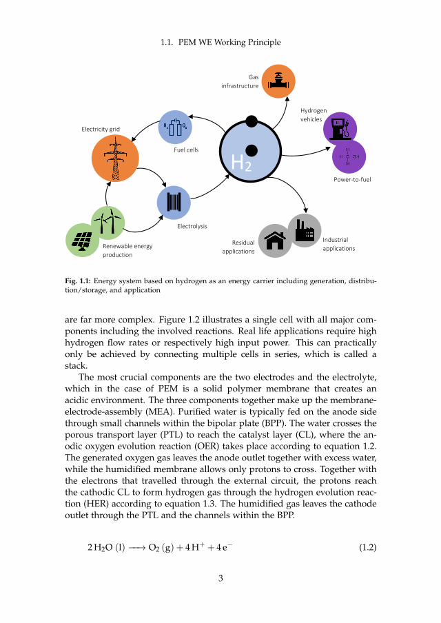
One technology that may address both issues at the same time is polymerelectrolyte membrane water electrolysis (PEM WE). During the electrolysisof water, hydrogen gas is produced that may be stored and utilized againto be converted back into electrical energy. This represents the long-termshift of production/consumption mismatch. The PEM technology specifi-cally exhibits certain features that also make it interesting for grid-stabilizingapplications as detailed in section 1.1). Additionally, hydrogen produced byrenewable energy powered electrolysis can be considered CO2 neutral andtherefore replace the state of the art process of natural gas reforming. Thehydrogen gas may also serve as a substitute for natural gas in certain appli-cations and therefore play an important role in all non-electrical applicationssuch as transportation, heating, and many other industrial uses. Figure 1.1illustrates an energy system that is based on hydrogen.
1.1 PEM WE Working Principle
The fundamentals of water electrolysis as well as the specifics of the PEMtechnology are describes in more detail in this section. Water electrolysis isa well known process that dates back to 1866 with the invention of the Hof-mann voltameter [47]. It describes the process of electrochemically splittingwater into its components hydrogen and oxygen as seen in equation 1.1:
2 H2O −−→ 2 H2 + O2 (1.1)
Although the main principle remains the same, modern electrolysis plants
2
1.1. PEM WE Working Principle
Hydrogen vehicles
Power-to-fuel
Gas infrastructure
Industrial applications Renewable energy
production
Fuel cells
Electrolysis
Electricity grid
Residual applications
H2
Fig. 1.1: Energy system based on hydrogen as an energy carrier including generation, distribu-tion/storage, and application
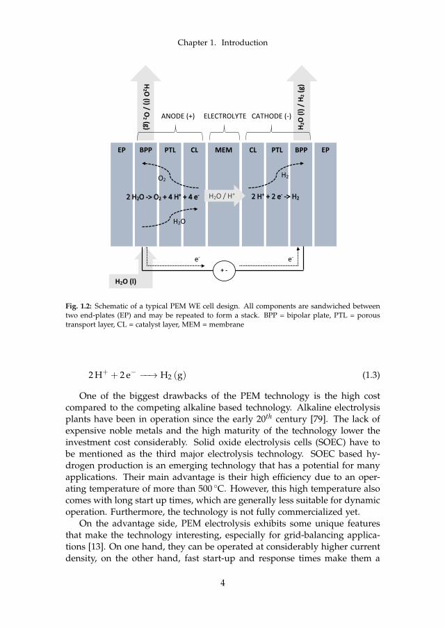
are far more complex. Figure 1.2 illustrates a single cell with all major com-ponents including the involved reactions. Real life applications require highhydrogen flow rates or respectively high input power. This can practicallyonly be achieved by connecting multiple cells in series, which is called astack.
The most crucial components are the two electrodes and the electrolyte,which in the case of PEM is a solid polymer membrane that creates anacidic environment. The three components together make up the membrane-electrode-assembly (MEA). Purified water is typically fed on the anode sidethrough small channels within the bipolar plate (BPP). The water crosses theporous transport layer (PTL) to reach the catalyst layer (CL), where the an-odic oxygen evolution reaction (OER) takes place according to equation 1.2.The generated oxygen gas leaves the anode outlet together with excess water,while the humidified membrane allows only protons to cross. Together withthe electrons that travelled through the external circuit, the protons reachthe cathodic CL to form hydrogen gas through the hydrogen evolution reac-tion (HER) according to equation 1.3. The humidified gas leaves the cathodeoutlet through the PTL and the channels within the BPP.
2 H2O (l) −−→ O2 (g) + 4 H+ + 4 e− (1.2)
3
Chapter 1. Introduction
H2O (l)
PTL MEM CL CL
H2 O
(l) / O2 (g) H 2
O (l
) / H
2 (g)
ANODE (+) ELECTROLYTE CATHODE (-)
BPP EP PTL BPP EP
+ -
2 H2O -> O2 + 4 H+ + 4 e- 2 H+ + 2 e- -> H2
e- e-
H2O
O2 H2
H2O / H+
Fig. 1.2: Schematic of a typical PEM WE cell design. All components are sandwiched betweentwo end-plates (EP) and may be repeated to form a stack. BPP = bipolar plate, PTL = poroustransport layer, CL = catalyst layer, MEM = membrane
2 H+ + 2 e− −−→ H2 (g) (1.3)
One of the biggest drawbacks of the PEM technology is the high costcompared to the competing alkaline based technology. Alkaline electrolysisplants have been in operation since the early 20th century [79]. The lack ofexpensive noble metals and the high maturity of the technology lower theinvestment cost considerably. Solid oxide electrolysis cells (SOEC) have tobe mentioned as the third major electrolysis technology. SOEC based hy-drogen production is an emerging technology that has a potential for manyapplications. Their main advantage is their high efficiency due to an oper-ating temperature of more than 500 C. However, this high temperature alsocomes with long start up times, which are generally less suitable for dynamicoperation. Furthermore, the technology is not fully commercialized yet.
On the advantage side, PEM electrolysis exhibits some unique featuresthat make the technology interesting, especially for grid-balancing applica-tions [13]. On one hand, they can be operated at considerably higher currentdensity, on the other hand, fast start-up and response times make them a
4
1.1. PEM WE Working Principle
potent option for dynamic operation. However, sufficient lifetime at suchdynamic operation has yet to be proven. Due to its solid membrane, an-other unique feature of the PEM technology is the possibility to internallypressurize the gases. When it comes to hydrogen gas storage, pressurizedgas bottles of up to 700 bar are the most widely used option. A world-wideinfrastructure for bottle refilling and distribution is in place, which may bereviewed when it comes to up-scaling of the technology in the GW-range.Underground caverns holding the gas at around 20 to 200 bar could presenta feasible option for gas storage of that magnitude [33]. In both cases, hy-drogen has to be pressurized in order to achieve acceptable volume-to-massratios. Also direct utilization in industrial applications such as methanol pro-duction requires hydrogen at a certain pressure. This can be done by externalcompressors, which are readily available on the market. However, their en-ergy consumption would lower the overall system efficiency.
Internal pressurization within the stack can be done symmetrically, i.e.with both oxygen and hydrogen at the same output pressure, or asymmet-rically, where only the hydrogen side is pressurized. Systems with internalpressurization of up to 50 bar are available, while demonstrations of up to100 bar have been shown [50, 92]. This reduces the external compression de-mand or even makes it completely redundant, which lowers balance of plant(BoP) complexity.
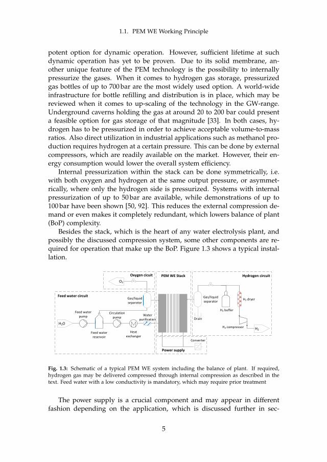
Besides the stack, which is the heart of any water electrolysis plant, andpossibly the discussed compression system, some other components are re-quired for operation that make up the BoP. Figure 1.3 shows a typical instal-lation.
Heat exchanger
Circulation pump
H2O
Feed water reservoir
Feed water pump
O2
H2 buffer
H2 compressor
Drain
Converter
H2
Water purification
H2 dryerGas/liquid separator
Gas/liquid separator
PEM WE Stack
Feed water circuit
Hydrogen circuit
Power supply
Oxygen cicuit
Fig. 1.3: Schematic of a typical PEM WE system including the balance of plant. If required,hydrogen gas may be delivered compressed through internal compression as described in thetext. Feed water with a low conductivity is mandatory, which may require prior treatment
The power supply is a crucial component and may appear in differentfashion depending on the application, which is discussed further in sec-
5
Chapter 1. Introduction
tion 1.2. Furthermore, the feed water may or may not be recirculated. Inboth cases it has to be highly purified, which may make further componentssuch as ion exchange filters necessary. The feed water circuit may also beutilized for heat management, where the water itself represents the coolingliquid. However, in real systems, external cooling is usually required. Bothgases can be stored in gas reservoirs or pressurized gas bottles, which makesit necessary to dry them beforehand. This is done in a gas/liquid separa-tor, while the oxygen is sometimes just vented into the atmosphere insteadof being utilized further. However, there is a potential market for oxygenutilization for example in medical applications [51].
1.2 Realistic Operation Scenarios
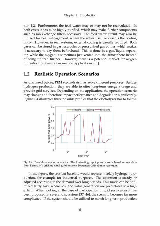
As discussed before, PEM electrolysis may serve different purposes. Besideshydrogen production, they are able to offer long-term energy storage andprovide grid services. Depending on the application, the operation scenariomay change and therefore impact performance and degradation significantly.Figure 1.4 illustrates three possible profiles that the electrolyzer has to follow.
30 60 90
time /min
0
0.2
0.4
0.6
0.8
1
1.2
norm
aliz
ed in
put p
ower
/-
constant cycling fluctuating
Fig. 1.4: Possible operation scenarios. The fluctuating input power case is based on real datafrom Denmark’s offshore wind turbines from September 2018 (5 min resolution)
In the figure, the constant baseline would represent solely hydrogen pro-duction, for example for industrial purposes. The operation is steady oradjusted according to the demand over long periods. This mode can be opti-mized fairly easy, where cost and value generation are predictable to a highextent. When looking at the case of participation in grid services as it hasbeen proposed in several discussions [37, 46], the scenario becomes far morecomplicated. If the system should be utilized to match long-term production
6
1.3. Motivation and Research Goals
and demand through hydrogen storage, the cycling case in figure 1.4 repre-sents a typical operation mode. In times of high production and low demand(e.g. strong winds during nighttime), the input power is very high in orderto absorb excess energy. At other times, the system runs on lower power ormay be switched off completely. This case is less predictable, but followscertain patterns such as day/night cycles. The system operator continues tobe able to sell hydrogen to industrial outlets or utilize it for feeding energyback to the grid during low production/high demand periods. Furthermore,the energy cost for the hydrogen production may be low due to the high ex-cess. Last but not least, providing grid services for frequency stability pushesthe operation scenario to a more extreme. Excess power is highly fluctuatingand little predictable. The fluctuating case in figure 1.4 illustrates a possibleprofile. Although the hydrogen production may not be as high as in the twoearlier cases, the major value generation in this scenario is to act as a gridservice provider. An extension of that are micro combined heat and power(µCHP) plants, which can be operated with intermittent hydrogen produc-tion to create a business case. A combination of any of the presented casesmay be considered when designing and optimizing a PEM WE system.
1.3 Motivation and Research Goals
The main motivation of this work is to investigate the possibilities of furtherincreasing the share of renewable energy sources within an electrical grid.The installed capacity of wind power in Denmark was 5.5 GW in 2017, whichrepresents a share of around 40% [20, 96]. In the past, the generated windpower exceeded the countries total consumption on several days as for ex-ample on the 9th and 10th of June 2015 [29]. Energy storage and ensuring astable grid frequency are crucial for a further increase in fluctuating energysources such as wind and solar energy. This work contributes by evaluatingthe possibility of utilizing PEM WE systems in an electrical grid for the pre-sented purposes of energy storage and providing grid services, where oneof the major issues is the lifetime under dynamic operation. The problem isaddressed firstly by an experimental approach on single cells, and secondlyby a lifetime simulation with the membrane being the restrictive component.The main objectives can be summarized as:
• Identify the most crucial operational parameters and their impact onPEM WE performance degradation
• Evaluate the suitability of PEM WE in highly dynamic operation sce-narios
• Develop a model that predicts the lifetime under several operating con-ditions
7

Chapter 1. Introduction
8
Chapter 2
State of the Art PEM WEDegradation
This chapter introduces the state of the art of PEM WE while focusing onissues related to degradation. The discussion is separated into the maincomponents membrane, catalyst, and others. Besides the given references,a good review of PEM WE performance and critical research gaps can befound in [7, 16]. To start with, the featured terminology as used in this workis clarified.
Quality is defined by the extent a product fulfills the advertised qualitiesat the beginning of life. In the case of PEM WE that may be an efficiency, gaspurity, or alike. These parameters may suffer from degradation related to ag-ing throughout its time of use, where degradation is separated into reversibleand irreversible decrease in performance. The ability to maintain BoL per-formance to a certain degree is called reliability, with durability usually refer-ring to irreversible processes, whereas stability describes the ability to recoverfrom reversible losses [36]. When degradation or sudden catastrophic failurecauses the product to not meet the requirements for the specific applicationanymore, the product can be said to have reached its end of life (EoL). To theauthor’s best knowledge, no standards define the EoL for PEM WE further.However, for PEM WE as for PEM FC, the EoL can be caused by three mainreasons: technical, safety-related, and economical [25]. A technical EoL couldbe to fail meeting the required gas production rate, while safety-related is-sues include the creation of explosive hydrogen-oxygen mixtures. Lastly, ifthe hydrogen production cost is getting too high due to an efficiency loss,an economical EoL is reached. It should be noted, that reaching one EoLcriteria in one application does not automatically exclude the system fromperforming sufficiently well in another application.
9
Chapter 2. State of the Art PEM WE Degradation
2.1 Characterization Techniques
Due to the high similarity between PEM WE and FC, the most commonlyapplied characterization methods are virtually the same and therefore wellestablished [58]. However, there are important differences in their practi-cal application and analysis. The major methods used in this work are po-larization curves (IV), electrochemical impedance spectroscopy (EIS), cyclicvoltammetry (CV), and scanning electron microscopy (SEM) and are shortlyintroduced in this section.
Polarization curves are the most straight forward method to quicklyevaluate the overall cell performance. In potentiostatic mode, the curve isconstructed by imposing a voltage and measuring the current, the galvano-static mode describes the other way round. Sensitive parameters are theresolution of data points, the dwell time at each operation point, and accu-racy of the measuring device. If all are chosen appropriately, the data mayalready reveal in-depth information about the cell. This includes informa-tion about involved voltage losses which may be connected to the differentreaction mechanisms and components (see also section 2.4). The data maybe presented in IV curves, where the voltage is typically plotted against thecurrent density, or in Tafel plots, where usually the overpotential is plottedagainst the logarithmic current density. However, to draw more confidentand meaningful conclusions, polarization data cannot serve as the sole char-acterization method. Furthermore, the technique can be disruptive whenstudying degradation since the recording of the curve involves changing theoperation to a high extend.
Electrochemical impedance spectroscopy is a non-disruptive alterna-tive to IV curves to characterize a cell. It should be noted that these twomethods can co-exist, but not replace each other. EIS has far more potentialto gain insight into electrochemical systems compared to simple polarizationmeasurements, at the cost of much higher complexity for the equipment aswell as the analysis. Generally, an AC disturbance signal is super-imposed ona DC bias signal, while the response is recorded. As IV curves, the methodcan be applied potentio- or galvanostatically, where in both cases the mainparameter for optimization is the magnitude of the disturbance signal, thatbalances between noise reduction (achieved through high disturbance signalmagnitude) and ensuring steady state operation (achieved through low dis-turbance signal magnitude). The signal is imposed at various frequencies,which makes it possible to connect the response to certain components orelectrochemical processes. For that purpose, a helpful tool for the analysisis to fit the data to an electrical equivalent circuit (EEC). However, EIS is a
10
2.2. Degradation Mechanisms
highly complex technique, and the fitting process has to be done with cau-tion, since it is prone to wrong conclusions.
Cyclic voltammetry is a versatile tool that plays an important role inmany branches of fundamental and applied electrochemical research, wherethe data is shown in a cyclic voltammogram. A potentiostat records thecurrent while an imposed voltage is swept between two limits. Attention hasto be paid not only to the upper and lower voltage limit, but also to the scanrate. Typical applications in PEM WE research are for example investigationson catalyst performance.
Scanning electron microscopy is a destructive and therefore post-mortemcharacterization method. In SEM, images of high resolution can be obtainedby means of an electron beam. The major application within PEM researchis to examine the MEA’s cross section. The captured images reveal insightinto the different layers in terms of their thickness and geometrical struc-ture. When compared to a fresh sample, SEM presents an effective way toqualitatively and quantitatively evaluate degradation processes.
2.2 Degradation Mechanisms
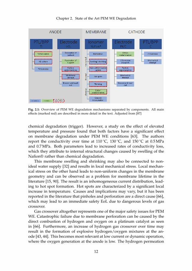
Figure 2.1 shows an overview of possible degradation mechanisms groupedinto the main components. The classification was done within the Euro-pean NOVEL project and presented at the Second International Workshop onDurability and Degradation Issues in PEM Electrolysis Cells and its Componentsin Freiburg in 2016 [68, 87]. The main effects (marked red in the figure) andsome other effects will be discussed in the following literature review. Acomprehensive review of PEM WE degradation can be found in [32].
2.2.1 Membrane
As seen in figure 2.1, membrane degradation can be classified into three maingroups: mechanical, thermal, and chemical. The analysis here focuses on thestate of the art perfluorosulfonicacid (PFSA) membranes such as Nafion® orAquivion® with thicknesses between 100 µm and 200 µm [7]. As the materialis the same, the mechanisms are equally valid for the ionomer within thecatalyst layers. Their implication will be discussed in section 2.2.2, whereasthis section focuses only on the impact on the membrane directly.
As long as the operating point remains below the melting point of thematerials, thermal degradation is usually more a result and a trigger ratherthan a mechanism. Inhomogeneities in thickness, catalyst activity, or thelike within the layers may cause hot spots (result), which in turn accelerate
11
Chapter 2. State of the Art PEM WE Degradation
Fig. 2.1: Overview of PEM WE degradation mechanisms separated by components. All maineffects (marked red) are described in more detail in the text. Adjusted from [87]
chemical degradation (trigger). However, a study on the effect of elevatedtemperature and pressure found that both factors have a significant effecton membrane degradation under PEM WE conditions [63]. The authorsreport the conductivity over time at 110 C, 130 C, and 150 C at 0.5 MPaand 0.7 MPa. Both parameters lead to increased rates of conductivity loss,which they attribute to internal structural changes caused by swelling of theNafion® rather than chemical degradation.
This membrane swelling and shrinking may also be connected to non-ideal water supply [32] and results in local mechanical stress. Local mechan-ical stress on the other hand leads to non-uniform changes in the membranegeometry and can be observed as a problem for membrane lifetime in theliterature [15, 90]. The result is an inhomogeneous current distribution, lead-ing to hot spot formation. Hot spots are characterized by a significant localincrease in temperature. Causes and implications may vary, but it has beenreported in the literature that pinholes and perforation are a direct cause [66],which may lead to an immediate safety EoL due to dangerous levels of gascrossover.
Gas crossover altogether represents one of the major safety issues for PEMWE. Catastrophic failure due to membrane perforation can be caused by thedirect combustion of hydrogen and oxygen on a platinum catalyst as seenin [66]. Furthermore, an increase of hydrogen gas crossover over time mayresult in the formation of explosive hydrogen/oxygen mixtures at the an-ode [43, 44]. This becomes most relevant at low current or dynamic operation,where the oxygen generation at the anode is low. The hydrogen permeation
12
2.2. Degradation Mechanisms
at low currents [94] can create an environment above the lower explosionlimit (LEL) of around 4vol-% hydrogen in air at 80 C [65]. Operation atasymmetric pressure condition (pcathode > panode) aggravates the issue due toincreased hydrogen permeation [95]. Oxygen crossover on the other handmay facilitate the formation of hydrogen peroxide, which in turn acceleratesmembrane degradation even more. Lastly, it decreases gas purity, resulting ina possible technical-EoL depending on the application [8]. Pinholes may alsobe the result of the PTL fibres piercing the membrane, which is directly cou-pled to the applied compression on the MEA [26, 32]. Additionally, high gaspressure operation enhances mechanical stress, where the main issue againbecomes gas crossover.
Finally, chemical membrane degradation is a lifetime limiting factor [32].The major mechanisms are based on metallic impurities that stem from theBoP, the feed water, or the MEA. One understanding is that cations such asFe2+ dissolve into the membrane, where they occupy ion exchange sites [85,93]. This lowers the proton conductivity and therefore increases the ohmicoverpotential, since protons cannot be transported effectively anymore. Thisprocess is shown to be reversible in the literature [93]; however, it requiresa complete disassembly of the cell or stack in order to access the MEA andimmerse it in sulfuric acid. Another source of metallic impurities are thecatalyst layers, where platinum particles have been observed to migrate intothe membrane [41]. However, the particles most likely originated from theanode side, where platinum is not a suitable catalyst material due to its highinstability within the voltage range. A much lower dissolution of the re-spective material is observed when switching to iridium or ruthenium basedoxides [4].
Apart from the described metal cation contamination, iron and othermetallic ions may also catalyze a reaction known as the Fenton reaction. It iswell known to cause membrane thinning in PEM FC and proven to also occurin PEM WE. As it is detailed in chapter 5, the reader is also referred there.In principle, radicals such as hydroxyl (HO•) and hydroperoxyl (HOO•) aregenerated in the presence of hydrogen peroxide (H2O2. Some of these rad-icals in turn attack the membrane, which can be observed through fluoride(F– ) release and thinning. The most common way to report fluoride release isthrough area-normalized emission rates (FER). This is done by determiningthe F– concentration in the effluent water. The reported order of magnitudeis between 1 · 10−1 and 1 · 101µg cm−2 h−1, where one of the most comprehen-sive datasets for PEM WE can be found in [34]. The authors found an impactof temperature, where the release rate roughly triples with an increase from60 C to 80 C. This is qualitatively and quantitatively in line with previousfindings [53]. More interestingly, they also found an impact of current densitywhich peaks between 0.2 A cm−2 to 0.4 A cm−2. The factor between the mini-mum and maximum FER is roughly two. At all times, the FER at the cathode
13
Chapter 2. State of the Art PEM WE Degradation
is by far higher compared to the anode. The authors furthermore found evi-dence through SEM that links the fluoride loss to membrane thinning. Mem-brane thinning through SEM without FER data was also identified by otherresearchers. The observed decrease was at times substantial and accountedfor around 50% [85] and up to 75% of the initial thickness [41]. Among thefirst published evidence for membrane material loss in WE applications datesback to 1998, where a stack was found to degrade inhomogeneously [90].
Theoretically, a thinner membrane leads to a decrease in ohmic resistance.The total ohmic resistance of the cell can be measured by means of EIS, wherea decrease of the high frequency intercept (HFR) in the Nyquist plane overtime is in fact observed by some researchers [4, 55, 85]. However, the dropin HFR is lower than what the thinning would suggest [85], and an increasein HFR over time is also reported in the literature [55, 75, 93]. Since theHFR is equivalent to the total ohmic resistance and not only the membraneresistance, that may be explained by a coupling of other phenomena thatincrease ohmic resistance. Among others, that may be the evolution of aoxide layer on the PTL as further explained in section 2.2.3. The problemwith membrane thinning through chemical attack is the above mentionedincrease in gas crossover that may lead to a technical or safety-related EoL.
2.2.2 Catalyst Layers
The state of the art catalyst materials are iridium-oxide (IrO2) at the anodeand carbon-supported platinum (Pt/C) at the cathode. Both layers have acontent of around 5% to 25% ionomer for binding purposes [10, 16]. There-fore, the binder may experience the same degradation phenomena as de-scribed in section 2.2.1 above. This may imply different mechanical issuessuch as a structural change within the CL, which may lead to a loss of perfor-mance [32]. Furthermore, ruthenium-based catalysts may be more efficientfor the OER, but IrO2 represents the best compromise between performanceand stability [31]. The same conclusion was also drawn by a screening ofdifferent materials, which were evaluated for stability by means of a cyclingvoltage profile [88].
The noble-metal loading is usually between 0.5 and 2 mg cm−2 for theanode and ≤1 mg cm−2 for the cathode [7, 16], while lower loading mayeffect stability [19]. However, low catalyst loading was successfully demon-strated by other researchers [11, 91]. Their Pt loading as low as 0.025 mg cm−2
achieved decent performance, while Ir loading was found to be optimalwithin 1 and 2 mg cm−2 due to homogeneity issues at the lower and masstransport limitations at the upper end. However, promising results are re-ported by [77], who reduced the IrO2 loading to 0.1 mg cm−2 without com-promising the performance. The authors claim that by adding a Ti-support,the ohmic resistance is decreased significantly and they achieved 1000 h with
14
2.2. Degradation Mechanisms
decent durability. The reported degradation rates of 180 µV h−1 with regu-lar loading and 20 µV h−1 with Ti-supported reduced loading, respectively,are contextualized to reported values in the literature in figure 2.2. TiC-supported Ir was also found to improve performance compared to unsup-ported Ir of up to one order of magnitude, which is connected to a lowerpolarization resistance due to improved deposition of particles [62]. How-ever, any support is again prone to their unique degradation potential suchas Ti-passivation is this case [89].
A general degradation issue connected to both the anode and cathodecatalyst is the loss of electrochemical surface area (ECSA) [32], which is con-nected to the geometrical area by the roughness factor. The ECSA can de-crease over time due to an agglomeration of catalyst particles and thereforean increase in mean particle size. In [76], the authors identified roughly adoubling in diameter at the cathode (Pt/C) through XRD and TEM analy-sis for constant and dynamic operation, while no change was observed atthe anode (IrO2). Although no reaction pathway for particle agglomerationhas been reported, similar underlying mechanisms as known from FC re-search are generally conceivable [89]. This includes coalescence (for examplethrough thermal sintering) and Ostwald ripening (through dissolution andredepositioning) [89]. Pt particle mobility has been found to be a function ofthe cathode potential [73], where a more negative potential leads to highermobility. At the same time, [76] found no Pt migrated to the anode or Ir tothe cathode at various long-term operation modes. At elevated voltages of>2.05 V vs. RHE as it may be the case for the PEM WE anode, the morevolatile species IrO3 can be formed and cause dissolution [89]. This can po-tentially also cause catalyst loss, which has been reported for Pt particles [41].Lastly, reversible cation contamination may temporarily decrease ECSA as re-ported by [93].
2.2.3 Other Components
One of the most severe challenges in PEM WE degradation is the harsh en-vironment especially at the anode. Low pH values of less than 4, elevatedtemperature of up to 80 C, and voltages of up to more than 2 V and more atthe presence of pure oxygen require materials with high resistance towardscorrosion [16, 32, 52]. Therefore, the stable but costly Ti became the standardmaterial for anode PTL and BPP [7], which makes the BPP the major con-tributor to the whole stack cost with around 50% (2010 and 2014 estimations)due to material and high machining cost for Ti [6, 12, 69]. However, even Tiis not immune towards aging and is reported to potentially contribute quitea share to the overall cell voltage increase over time. It is believed that ti-tanium develops an oxide layer on its surface, which on one hand protectsthe material from further corrosion, but on the other hand increases the in-
15
Chapter 2. State of the Art PEM WE Degradation
terfacial contact resistance (ICR) [7]. This hypothesis has been validated in along-term experiment, where the interfacial contact resistance (ICR) of the Ti-PTL before and after the test was compared. Since the ICR measurement wascarried out ex-situ, the result is qualitative, but the increase is observable,and the theory is in line with the reported increase in HFR over time [75].The authors repeated the experiment under the same conditions with a Pt-coated Ti-PTL that supposedly prevents the development of an oxide layer.The ICR remained almost constant, resulting in a much lower overall cellvoltage increase. This underlines the impact of PTL-passivation in PEM WEdegradation, and the possible mitigation through coatings, which has beenreported before [5]. However, Pt coatings are expensive to apply and increasematerial cost [52]. The same applies for coatings on stainless steel BPP [38].
Another issue is the hydrogen uptake by titanium at elevated potentialsand temperatures and the resulting embrittlement. However, the whole sys-tem is highly complex and the available literature lacks comprehensive stud-ies. Theoretically, if the hydrogen uptake exceeds a certain threshold of sol-ubility, a further uptake may result in cracks. However, the above describedpassivation layer should protect the Ti components against such, while hu-midity and pH value affect absorption abilities. On the other hand, fluorideions from the previously described membrane attack have the ability to attackthe oxide layer [32]. Therefore, hydrogen embrittlement in titanium compo-nents remains a topic of research, while at the same time alternative materialsand coatings are also investigated [52, 57].
Finally, Ti particles probably originating from the anode PTL have beenfound at the cathode electrode, where they effectively lower the exchangecurrent density over time [76].
2.3 Quantifying Voltage Degradation
Most of the previously discussed degradation phenomena have a direct im-pact on the cell voltage. Therefore, the evolution of the voltage at a certaincurrent over time is a suitable parameter for capturing the overall degrada-tion. It is potentially interesting for comparing different materials, cell de-signs, or operation modes. However, this voltage degradation rate has to beseen as a first figure and cannot serve as the sole indication for degradationand the end of life. One of the biggest problems connected to it is the lack ofstandardized protocols and clear definitions of how to calculate the parame-ter. Especially in the context of dynamic operation and variable applications,a time-based degradation rate has limited significance to describe the relevantdegradation. For example, a PEM WE system for energy storage operates ina very different pattern and has a different added value than one that mainlyoperates for industrial hydrogen production (see section 1.2). A molar-based
16
2.3. Quantifying Voltage Degradation
degradation rate that takes the hydrogen production into account is alreadymore flexible in order to asses performance loss and can be observed in theliterature [76]. The two numbers are convertible into each other as long asthe operation profile is known.
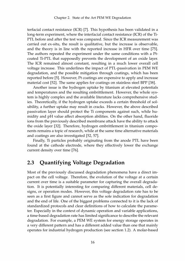
However, a review over the available literature that includes long-termvoltage degradation is a useful overview and can be a good starting pointto evaluate the most crucial parameters for degradation. An extraction ofthe most relevant literature can be found in table 4.2, where the outcomes ofthis work are put into context. Figure 2.2 shows the values of the completeconsidered dataset as a function of temperature and publication year. How-ever, the dataset contains experiments with considerably different conditionssuch as catalyst loading or active area. Furthermore, the degradation ratesare in most cases only reported for one current operation point. As it will beshown in chapter 4, the voltage degradation rate is dependent on the refer-ence current point. Nevertheless, the lack of a clear relationship exemplifiesthe difficulties of comparing quantitative data due to different test conditionsand the associated problems with reproducibility of data across the laborato-ries in the world. It does however indicate a trend, that voltage degradationrates rise with temperature. The vast majority of reported experiments wascarried out at 80 C, while only one was found above that. Although notclaiming completeness, the figure also indicates a risen interest in PEM WEdegradation as most data was collected within the past 5 years.
Fig. 2.2: Voltage degradation rates as a function of temperature and publication year as reportedin the literature
17
Chapter 2. State of the Art PEM WE Degradation
2.4 Modelling Approaches
PEM WE degradation models are very rare and in fact, only one was foundwithin the published literature in [17]. It addresses the issue of membranedegradation, where the authors present a 1D gas-crossover model and a setof ten electrochemical reactions, which simulate membrane attack and even-tually thinning. Finally, a lifetime prediction is given based on the criteriathat explosive gas mixtures cause a safety-related EoL. The approach is simi-lar to what can be found for PEM FC degradation models, of which few canbe found in the literature [40, 45, 82, 98]. Another FC membrane degradationmodel is based on empirical laws [18] and could be done similarly for WE.The authors investigated the effect of potential, pressure, and humidity onFER and turned the outcomes into empirical formulas. A system model thatfocuses on temperature-dependent degradation was developed throughoutthe LastEISys project at DLR [27], but further publicly available informationwas not found.
Additionally, several mathematical performance models are available [1,64], which can be implemented into degradation models after some adjust-ments. A good overview of performance modelling can be found in severalreview papers [2, 16, 72]. Furthermore, some 3D models for two-phase flowand bubble transport, which is specific for PEM WE, can be found [3, 71].Notably well investigated is high pressure operation including gas-crossoverat asymmetrical condition from cell to system level [8, 9, 42, 80, 81, 94, 95].This strongly supports the high relevance gas permeation plays in PEM WE.
18
Chapter 3
Investigations on PEM WEPerformance
Before studying degradation phenomena, characterization methods and theBoL performance were investigated. This chapter introduces the methodol-ogy, EIS peculiarities for PEM WE, and summarizes the findings throughoutthis PhD project connected to cell compression. Some results were publishedin peer-reviewed outlets as shown in the outline (papers [A], [X1], and [X2]).
3.1 MEA Characteristics and Production
Throughout the project, two different types of cells were used for the exper-iments as described here. The MEA production protocol has been reportedto have an effect on performance and degradation [85], which makes it arelevant parameter for comparison.
Cell type I Nafion® 117 served as the solid electrolyte for the small cellswith 2.89 cm2 active area. As the MEAs were provided by EWII Fuel CellsA/S, Denmark, no further information on the production method is known.However, the anode and cathode catalyst layers consisted of 0.3 mg cm−2
IrO2 and 0.5 mg cm−2 Pt/C, respectively. Additionally, the anode exhibited ametallic Ir layer with a loading of 2.48 mg cm−2. A Ti-felt of 350 µm and 81%porosity, and Sigracet® 35DC carbon-paper were used as PTLs. The MEAswere investigated in the setup seen in figure 3.1a. The feed water was recir-culated at 270 mL min−1 (around 93 mL min−1 cm−2). This represents a highoverstoichiometry to ensure decent temperature control, which is solely doneby the pre-heated feed water itself.
19
Chapter 3. Investigations on PEM WE Performance
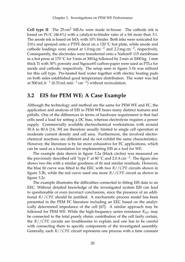
Cell type II The 25 cm2 MEAs were made in-house. The cathode ink isbased on Pt/C (46.6%) with a catalyst-to-binder ratio of a bit more than 3:1.The anode ink is based on IrO2 with 10% binder. Both inks were sonicated for210 s and sprayed onto a PTFE decal on a 120 C hot plate, while anode andcathode loadings were aimed at 1.0 mg cm−2 and 2.2 mg cm−2, respectively.Consequently, the electrodes were transferred onto a Nafion® 115 membranein a hot press at 170 C for 5 min at 300 kg followed by 2 min at 2000 kg. 1 mmthick Ti with 30% porosity and Sigracet® carbon-paper were used as PTLs foranode and cathode, respectively. The setup seen in figure 3.1b was utilizedfor this cell type. Pre-heated feed water together with electric heating padson both sides established good temperature distribution. The water was fedat 500 mL h−1 (0.33 mL min−1 cm−2) without recirculation.
3.2 EIS for PEM WE: A Case Example
Although the technology and method are the same for PEM WE and FC, theapplication and analysis of EIS in PEM WE bears many distinct features andpitfalls. One of the differences in terms of hardware requirement is that fuelcells need a load for setting a DC bias, whereas electrolysis requires a powersupply. Commercially available electrochemical workstations with around30 A to 80 A [14, 39] are therefore usually limited to single cell operation atmoderate current density and cell area. Furthermore, the involved electro-chemical reactions are different and do not exhibit the same characteristics.However, the literature is by far more exhaustive for FC applications, whichcan be used as a foundation for implementing EIS as a tool for WE.
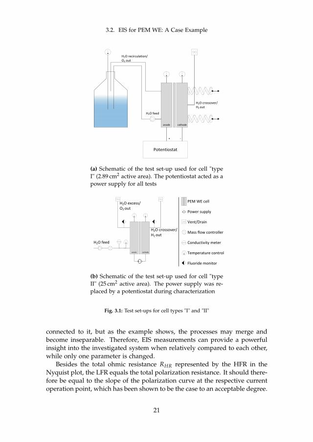
The example data shown in figure 3.2a (black circles) was measured onthe previously described cell "type I" at 80 C and 2.0 A cm−2. The figure alsoshows two fits with a similar goodness of fit and similar residuals. However,the blue fit curve was fitted to the EEC with two R//CPE circuits shown infigure 3.2b, while the red curve used one more R//CPE circuit as shown infigure 3.2c.
The example illustrates the difficulties connected to fitting EIS data to anEEC. Without detailed knowledge of the investigated system EIS can leadto questionable or even incorrect conclusions, since the presence of an addi-tional R//CPE should be justified. A mechanistic process model has beenpresented in the PEM FC literature including an EEC based on the analyt-ically determined impedance of the cell [67]. A similar approach may befollowed for PEM WE. While the high-frequency series resistance RHF maybe connected to the total purely ohmic contribution of the cell fairly certain,the R//CPE circuits are troublesome to explain and one has to be carefulwith connecting them to specific components of the investigated assembly.Generally, each R//CPE circuit represents one process with a time constant
20
3.2. EIS for PEM WE: A Case Example
anode cathode
Potentiostat
+ ‐
H2O crossover/ H2 out
H2O feed
H2O recirculation/O2 out
(a) Schematic of the test set-up used for cell "typeI" (2.89 cm2 active area). The potentiostat acted as apower supply for all tests
anode cathode
H2O crossover/ H2 out
H2O feed
H2O excess/ O2 out
PEM WE cell
Power supply
Vent/Drain
Mass flow controller
Conductivity meter
Temperature control
Fluoride monitor
(b) Schematic of the test set-up used for cell "typeII" (25 cm2 active area). The power supply was re-placed by a potentiostat during characterization
Fig. 3.1: Test set-ups for cell types "I" and "II"
connected to it, but as the example shows, the processes may merge andbecome inseparable. Therefore, EIS measurements can provide a powerfulinsight into the investigated system when relatively compared to each other,while only one parameter is changed.
Besides the total ohmic resistance RHR represented by the HFR in theNyquist plot, the LFR equals the total polarization resistance. It should there-fore be equal to the slope of the polarization curve at the respective currentoperation point, which has been shown to be the case to an acceptable degree.
21
Chapter 3. Investigations on PEM WE Performance
(a) EIS data fit based on the two EEC shown below. The similar fits may lead todifferent conclusions depending on the chosen EEC
R_HF
R1
CPE1 CPE2
R2
L_stray
(b) EEC with a series resis-tance and two R//CPE cir-cuits
R_HF
R1
CPE1 CPE2
R2
L_stray
CPE3
R3
(c) EEC with a series resis-tance and three R//CPE cir-cuits
Fig. 3.2: Electrochemical impedance spectroscopy (EIS) based on electrical equivalent circuits(EEC)
3.3 Impact of MEA Compression on Cell Perfor-mance
The cell compression is a crucial parameter and impacts both performanceand degradation. First and foremost, the BoL performance is a function ofMEA compression and should therefore be reported to enable meaningfulcomparison throughout the literature. However, that is often not the caseand moreover the literature lacks studies on the impact of PEM WE cellcompression. Within this PhD project, the effect of compression was exper-imentally investigated on a single cell as shown in paper [A]. The 2.89 cm2
state-of-the-art cell as described in section 3.1 ("type I") was electrochemicallycharacterized at its BoL in the set-up shown in figure 3.1a.
The temperature was held constant at 60 C and 80 C through the feedwater, whereas no other equipment than a potentiostat was used as a powersupply. Four die springs were used to control the compression in eight steps
22
3.3. Impact of MEA Compression on Cell Performance
as shown in table 3.1.
step # 0 1 2 3 4 5 6 7c /MPa 0.77 1.15 1.53 1.92 2.30 2.68 3.06 3.45
Table 3.1: Compression steps
The compression pressure Pc was calculated according to equation 3.1 andvalidated in an assembled cell through pressure-sensitive film.
Pc =Fs
A=
Rs · xA
(3.1)
In the equation, A represents the compressed area, and Fs the compressionforce exerted by the springs which is given by the spring constant Rs and thedisplacement x.
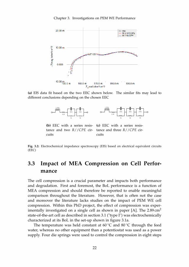
At each compression step, an IV curve and EIS measurements at variouscurrent densities were carried out at both temperatures. Figure 3.3 shows theHFR and LFR at 1.0 A cm−2 as a function of compression.
0.5 1 1.5 2 2.5 3 3.5
c /MPa
0.15
0.2
0.25
0.3
0.35
R /
*cm
2
HFR 60°CHFR 80°CLFR 60°CLFR 80°C
Fig. 3.3: High- and low-frequency intercepts at two temperatures as a function of cell compres-sion. Source: [A]
While the total ohmic resistance represented by the HFR decreases withtemperature is connected to higher Nafion® conductivity, the decrease withcompression is related to improved contacts. The order of magnitude of theeffect is similar for both parameters, where a temperature rise by 20 C de-creases the HFR by around 15% and an increase in compression by 2.68 MParesults in a 20% drop in HFR. To facilitate the analysis, the following resultsrefer to the measurements at 60 C.
23
Chapter 3. Investigations on PEM WE Performance
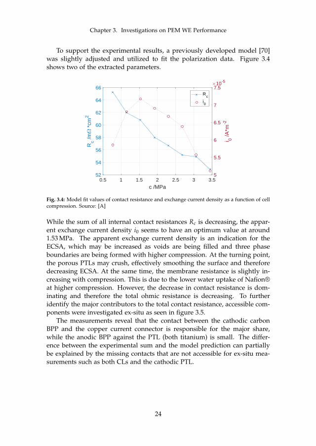
To support the experimental results, a previously developed model [70]was slightly adjusted and utilized to fit the polarization data. Figure 3.4shows two of the extracted parameters.
0.5 1 1.5 2 2.5 3 3.5
c /MPa
52
54
56
58
60
62
64
66R
c /m *
cm2
5
5.5
6
6.5
7
7.5
i 0 /A
*m-2
10-5
Rc
i0
Fig. 3.4: Model fit values of contact resistance and exchange current density as a function of cellcompression. Source: [A]
While the sum of all internal contact resistances Rc is decreasing, the appar-ent exchange current density i0 seems to have an optimum value at around1.53 MPa. The apparent exchange current density is an indication for theECSA, which may be increased as voids are being filled and three phaseboundaries are being formed with higher compression. At the turning point,the porous PTLs may crush, effectively smoothing the surface and thereforedecreasing ECSA. At the same time, the membrane resistance is slightly in-creasing with compression. This is due to the lower water uptake of Nafion®at higher compression. However, the decrease in contact resistance is dom-inating and therefore the total ohmic resistance is decreasing. To furtheridentify the major contributors to the total contact resistance, accessible com-ponents were investigated ex-situ as seen in figure 3.5.
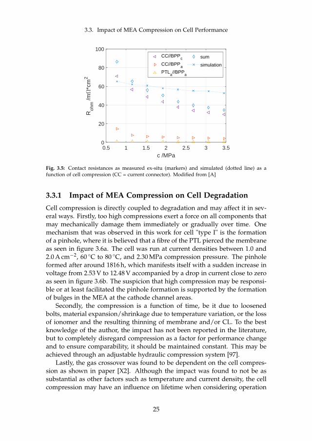
The measurements reveal that the contact between the cathodic carbonBPP and the copper current connector is responsible for the major share,while the anodic BPP against the PTL (both titanium) is small. The differ-ence between the experimental sum and the model prediction can partiallybe explained by the missing contacts that are not accessible for ex-situ mea-surements such as both CLs and the cathodic PTL.
24
3.3. Impact of MEA Compression on Cell Performance
0.5 1 1.5 2 2.5 3 3.5
c /MPa
0
20
40
60
80
100
Roh
m /m
*cm
2
CC//BPPc
CC//BPPa
PTLa//BPP
a
sum
simulation
Fig. 3.5: Contact resistances as measured ex-situ (markers) and simulated (dotted line) as afunction of cell compression (CC = current connector). Modified from [A]
3.3.1 Impact of MEA Compression on Cell Degradation
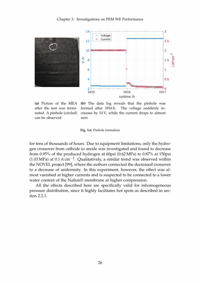
Cell compression is directly coupled to degradation and may affect it in sev-eral ways. Firstly, too high compressions exert a force on all components thatmay mechanically damage them immediately or gradually over time. Onemechanism that was observed in this work for cell "type I" is the formationof a pinhole, where it is believed that a fibre of the PTL pierced the membraneas seen in figure 3.6a. The cell was run at current densities between 1.0 and2.0 A cm−2, 60 C to 80 C, and 2.30 MPa compression pressure. The pinholeformed after around 1816 h, which manifests itself with a sudden increase involtage from 2.53 V to 12.48 V accompanied by a drop in current close to zeroas seen in figure 3.6b. The suspicion that high compression may be responsi-ble or at least facilitated the pinhole formation is supported by the formationof bulges in the MEA at the cathode channel areas.
Secondly, the compression is a function of time, be it due to loosenedbolts, material expansion/shrinkage due to temperature variation, or the lossof ionomer and the resulting thinning of membrane and/or CL. To the bestknowledge of the author, the impact has not been reported in the literature,but to completely disregard compression as a factor for performance changeand to ensure comparability, it should be maintained constant. This may beachieved through an adjustable hydraulic compression system [97].
Lastly, the gas crossover was found to be dependent on the cell compres-sion as shown in paper [X2]. Although the impact was found to not be assubstantial as other factors such as temperature and current density, the cellcompression may have an influence on lifetime when considering operation
25
Chapter 3. Investigations on PEM WE Performance
(a) Picture of the MEAafter the test was termi-nated. A pinhole (circled)can be observed
1815 1816 1817
runtime /h
2
4
6
8
10
12
14
V /V
0
0.5
1
1.5
2
2.5
3
i /A
*cm
-2
VoltageCurrent
(b) The data log reveals that the pinhole wasformed after 1816 h. The voltage suddenly in-creases by 10 V, while the current drops to almostzero
Fig. 3.6: Pinhole formation
for tens of thousands of hours. Due to equipment limitations, only the hydro-gen crossover from cathode to anode was investigated and found to decreasefrom 0.95% of the produced hydrogen at 60psi (0.62 MPa) to 0.87% at 150psi(1.03 MPa) at 0.1 A cm−2. Qualitatively, a similar trend was observed withinthe NOVEL project [99], where the authors connected the decreased crossoverto a decrease of uniformity. In this experiment, however, the effect was al-most vanished at higher currents and is suspected to be connected to a lowerwater content of the Nafion® membrane at higher compression.
All the effects described here are specifically valid for inhomogeneouspressure distribution, since it highly facilitates hot spots as described in sec-tion 2.2.1.
26
Chapter 4
Long Term PEM WEDegradation
This chapter summarizes the findings of the experimental investigations oncell degradation. The analysis includes the effect of operating parameters,a possible link to break-in mechanisms, and reversible versus irreversiblevoltage increase. The results were partly published in peer-reviewed outletsor presented at conferences (see thesis outline publications [B], [C], [C3]).
4.1 Activation Phase Phenomena
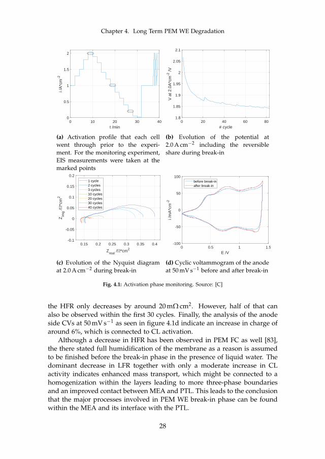
An initial performance gain can be observed in many PEM WE cells. Toshed some light onto the involved mechanisms, a 25 cm2 cell of "type II"as previously described was assembled and monitored for the first 60 h ofoperation. For these tests, the profile shown in figure 4.1a was applied. Theprofile consisted of current steps of 120 s each between 0.0 and 2.0 A cm−2,followed by 300 s at 1.0 A cm−2, and eventually a fast cycling period with10 s steps between 1.0 and 2.0 A cm−2. The whole cycle is repeated 83 times,which is equivalent to around 60 h. EIS spectra were recorded in each cycleat the marked points at 0.2, 1.0, and 2.0 A cm−2.
The potential at 2.0 A cm−2 after each cycle of about 40 min is plottedin figure 4.1b. A steep drop in potential from around 2.07 to 1.88 V can beobserved within the first 21 cycles. After that, the potential continues todecrease much slower down to 1.84 V after 83 cycles, which represented theend of the break-in phase. To get more insight into the cause of potentialdrop, figure 4.1c shows the Nyquist plot at the same operation point. Theextracted LFR drops significantly within the first 30 cycles, after which itstabilize. While the LFR experiences a total decrease of around 230 mΩ cm2,
27
Chapter 4. Long Term PEM WE Degradation
0 10 20 30 40
t /min
0
0.5
1
1.5
2
i /A
*cm
-2
(a) Activation profile that each cellwent through prior to the experi-ment. For the monitoring experiment,EIS measurements were taken at themarked points
0 20 40 60 80
# cycle
1.8
1.85
1.9
1.95
2
2.05
2.1
V a
t 2.0
A*c
m-2
/V
(b) Evolution of the potential at2.0 A cm−2 including the reversibleshare during break-in
0.15 0.2 0.25 0.3 0.35 0.4
Zreal
/ *cm2
-0.1
-0.05
0
0.05
0.1
0.15
0.2
Zim
g /
*cm
2
1 cycle2 cycles3 cycles10 cycles20 cycles30 cycles40 cycles
(c) Evolution of the Nyquist diagramat 2.0 A cm−2 during break-in
0 0.5 1 1.5
E /V
-100
-50
0
50
100
i /m
A*c
m-2
before break-inafter break-in
(d) Cyclic voltammogram of the anodeat 50 mV s−1 before and after break-in
Fig. 4.1: Activation phase monitoring. Source: [C]
the HFR only decreases by around 20 mΩ cm2. However, half of that canalso be observed within the first 30 cycles. Finally, the analysis of the anodeside CVs at 50 mV s−1 as seen in figure 4.1d indicate an increase in charge ofaround 6%, which is connected to CL activation.
Although a decrease in HFR has been observed in PEM FC as well [83],the there stated full humidification of the membrane as a reason is assumedto be finished before the break-in phase in the presence of liquid water. Thedominant decrease in LFR together with only a moderate increase in CLactivity indicates enhanced mass transport, which might be connected to ahomogenization within the layers leading to more three-phase boundariesand an improved contact between MEA and PTL. This leads to the conclusionthat the major processes involved in PEM WE break-in phase can be foundwithin the MEA and its interface with the PTL.
28
4.2. Reversible Voltage Increase
4.2 Reversible Voltage Increase
A long-term test of around 1800 h has been carried out on the small single cellwith 2.89 cm2 active area design as previously described (section 3.1, "typeI"). The cell was run at different currents and temperatures at a compressionpressure of 2.30 MPa, where the feed water was recirculated at 270 mL min−1.One of the main differences to most cells described in the literature is theinterdigitated anodic flow field design, which was implemented to enhanceperformance.
In the first 504 h of operation, where the cell was held constant at 1.5 A cm−2
and 60 C, the only interruption was a characterization phase every 24 h. Eachcharacterization phase included an IV curve from 0.01 A cm−2 to 3.0 A cm−2
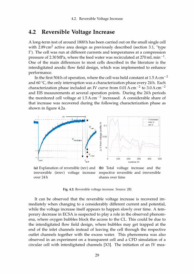
and EIS measurements at several operation points. During the 24 h periodsthe monitored cell voltage at 1.5 A cm−2 increased. A considerable share ofthat increase was recovered during the following characterization phase asshown in figure 4.2a.
(a) Explanation of reversible (rev) andirreversible (irrev) voltage increaseover 24 h
0 100 200 300 400 500
runtime /h
0
0.05
0.1
V fr
om v
olta
ge p
rofil
e /V
V increaseirrev Vrev V
(b) Total voltage increase and therespective reversible and irreversibleshares over time
Fig. 4.2: Reversible voltage increase. Source: [B]
It can be observed that the reversible voltage increase is recovered im-mediately when changing to a considerably different current and potential,while the voltage increase itself appears to happen slowly over time. A tem-porary decrease in ECSA is suspected to play a role in the observed phenom-ena, where oxygen bubbles block the access to the CL. This could be due tothe interdigitated flow field design, where bubbles may get trapped at theend of the inlet channels instead of leaving the cell through the respectiveoutlet channels together with the excess water. This phenomena was alsoobserved in an experiment on a transparent cell and a CFD simulation of acircular cell with interdigitated channels [X3]. The initiation of an IV mea-
29
Chapter 4. Long Term PEM WE Degradation
surement at low current and therefore low oxygen production may act as aflush for these bubbles, leaving a fully accessible CL behind again, whichleads to a voltage drop down to the initial potential plus irreversible losses.Although the share of the reversible increase does not follow any obvioustrend, the total gain during 24 h in absolute numbers is decreasing over timeas shown in figure 4.2b.
4.3 Irreversible Degradation under Different Op-eration Modes
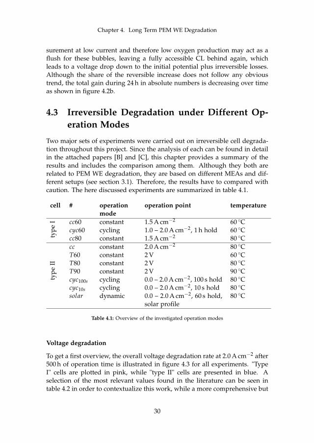
Two major sets of experiments were carried out on irreversible cell degrada-tion throughout this project. Since the analysis of each can be found in detailin the attached papers [B] and [C], this chapter provides a summary of theresults and includes the comparison among them. Although they both arerelated to PEM WE degradation, they are based on different MEAs and dif-ferent setups (see section 3.1). Therefore, the results have to compared withcaution. The here discussed experiments are summarized in table 4.1.
cell # operationmode
operation point temperature
type
I cc60 constant 1.5 A cm−2 60 Ccyc60 cycling 1.0 – 2.0 A cm−2, 1 h hold 60 Ccc80 constant 1.5 A cm−2 80 C
type
II
cc constant 2.0 A cm−2 80 CT60 constant 2 V 60 CT80 constant 2 V 80 CT90 constant 2 V 90 Ccyc100s cycling 0.0 – 2.0 A cm−2, 100 s hold 80 Ccyc10s cycling 0.0 – 2.0 A cm−2, 10 s hold 80 Csolar dynamic 0.0 – 2.0 A cm−2, 60 s hold,
solar profile80 C
Table 4.1: Overview of the investigated operation modes
Voltage degradation
To get a first overview, the overall voltage degradation rate at 2.0 A cm−2 after500 h of operation time is illustrated in figure 4.3 for all experiments. "TypeI" cells are plotted in pink, while "type II" cells are presented in blue. Aselection of the most relevant values found in the literature can be seen intable 4.2 in order to contextualize this work, while a more comprehensive but
30
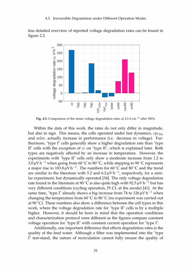
4.3. Irreversible Degradation under Different Operation Modes
less detailed overview of reported voltage degradation rates can be found infigure 2.2.
cc
T60
T80
T90
cyc 10
0s
cyc 10
s
sola
r
cc60
cyc6
0
cc80
-50
0
50
100
150
200
250
300
volta
ge d
egra
datio
n ra
te /
V*h
-1
Fig. 4.3: Comparison of the mean voltage degradation rates at 2.0 A cm−2 after 500 h
Within the data of this work, the rates do not only differ in magnitude,but also in sign. This means, the cells operated under fast dynamics, cyc10sand solar, actually increase in performance (i.e. decrease in voltage). Fur-thermore, "type I" cells generally show a higher degradation rate than "typeII" cells with the exception of cc on "type II", which is explained later. Bothtypes are negatively affected by an increase in temperature. However, theexperiments with "type II" cells only show a moderate increase from 1.2 to3.0 µV h−1 when going from 60 C to 80 C, while stepping to 90 C representsa major rise to 183.8 µV h−1. The numbers for 60 C and 80 C and the trendare similar to the literature with 5.2 and 6.2 µV h−1, respectively, for a simi-lar experiment, but dynamically operated [34]. The only voltage degradationrate found in the literature at 90 C is also quite high with 92.5 µV h−1 but hasvery different conditions (cycling operation, Pt CL at the anode) [41]. At thesame time, "type I" already shows a big increase from 74 to 126 µV h−1 whenchanging the temperature from 60 C to 80 C (no experiment was carried outat 90 C). These numbers also show a difference between the cell types in thiswork, where the voltage degradation rate for "type II" cells is by a multiplehigher. However, it should be born in mind that the operation conditionsand characterization protocol were different as the figures compare constantvoltage operation for "type II" with constant current operation for "type I".
Additionally, one important difference that effects degradation rates is thequality of the feed water. Although a filter was implemented into the "typeI" test-stand, the nature of recirculation cannot fully ensure the quality of
31
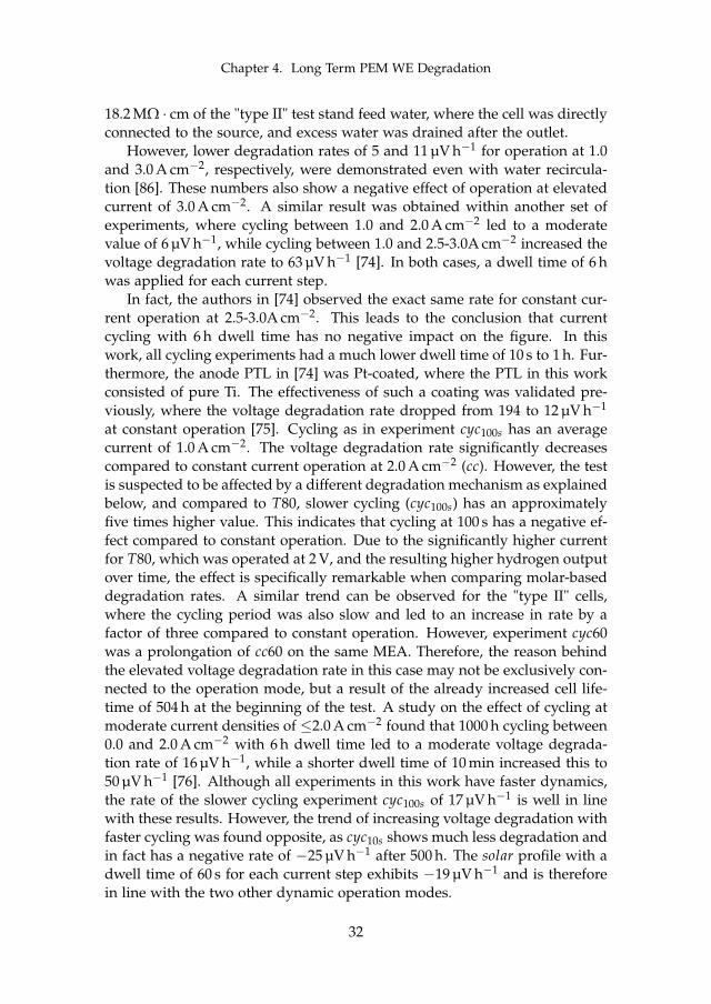
Chapter 4. Long Term PEM WE Degradation
18.2 MΩ · cm of the "type II" test stand feed water, where the cell was directlyconnected to the source, and excess water was drained after the outlet.
However, lower degradation rates of 5 and 11 µV h−1 for operation at 1.0and 3.0 A cm−2, respectively, were demonstrated even with water recircula-tion [86]. These numbers also show a negative effect of operation at elevatedcurrent of 3.0 A cm−2. A similar result was obtained within another set ofexperiments, where cycling between 1.0 and 2.0 A cm−2 led to a moderatevalue of 6 µV h−1, while cycling between 1.0 and 2.5-3.0A cm−2 increased thevoltage degradation rate to 63 µV h−1 [74]. In both cases, a dwell time of 6 hwas applied for each current step.
In fact, the authors in [74] observed the exact same rate for constant cur-rent operation at 2.5-3.0A cm−2. This leads to the conclusion that currentcycling with 6 h dwell time has no negative impact on the figure. In thiswork, all cycling experiments had a much lower dwell time of 10 s to 1 h. Fur-thermore, the anode PTL in [74] was Pt-coated, where the PTL in this workconsisted of pure Ti. The effectiveness of such a coating was validated pre-viously, where the voltage degradation rate dropped from 194 to 12 µV h−1
at constant operation [75]. Cycling as in experiment cyc100s has an averagecurrent of 1.0 A cm−2. The voltage degradation rate significantly decreasescompared to constant current operation at 2.0 A cm−2 (cc). However, the testis suspected to be affected by a different degradation mechanism as explainedbelow, and compared to T80, slower cycling (cyc100s) has an approximatelyfive times higher value. This indicates that cycling at 100 s has a negative ef-fect compared to constant operation. Due to the significantly higher currentfor T80, which was operated at 2 V, and the resulting higher hydrogen outputover time, the effect is specifically remarkable when comparing molar-baseddegradation rates. A similar trend can be observed for the "type II" cells,where the cycling period was also slow and led to an increase in rate by afactor of three compared to constant operation. However, experiment cyc60was a prolongation of cc60 on the same MEA. Therefore, the reason behindthe elevated voltage degradation rate in this case may not be exclusively con-nected to the operation mode, but a result of the already increased cell life-time of 504 h at the beginning of the test. A study on the effect of cycling atmoderate current densities of ≤2.0 A cm−2 found that 1000 h cycling between0.0 and 2.0 A cm−2 with 6 h dwell time led to a moderate voltage degrada-tion rate of 16 µV h−1, while a shorter dwell time of 10 min increased this to50 µV h−1 [76]. Although all experiments in this work have faster dynamics,the rate of the slower cycling experiment cyc100s of 17 µV h−1 is well in linewith these results. However, the trend of increasing voltage degradation withfaster cycling was found opposite, as cyc10s shows much less degradation andin fact has a negative rate of −25 µV h−1 after 500 h. The solar profile with adwell time of 60 s for each current step exhibits −19 µV h−1 and is thereforein line with the two other dynamic operation modes.
32
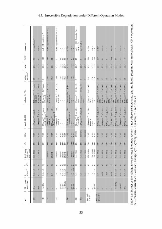
4.3. Irreversible Degradation under Different Operation Modes
ref
OP
mod
e(d
wel
lti
me)
i /Acm−
2T /
Cfe
edw
ater
/mL
min−
1
(/M
Ω×
cm)
t/h
MEM
anod
eC
L,PT
Lca
thod
eC
L,PT
Lac
tive
area
/cm
2ye
ar/µ
Vh−
1co
mm
ents
[35]
dyn
0.2.
..1.
060
3.33
(18.
2)10
00N
117
1.99
mg
cm−
2Ir
O2,
Ti1.
31m
gcm−
2Pt
blac
k,SG
L-24
BC25
2016
5.2
aver
age
1A
cm−
2
dyn
0.2.
..1.
080
3.33
(18.
2)10
00N
117
1.94
mg
cm−
2Ir
O2,
Ti1.
19m
gcm−
2Pt
blac
k,SG
L-24
BC25
2016
6.2
—”
—
[41]
cyc
(10h
)0.
0...
1.0
9040
00N
115
2.5m
gcm−
2Pt
unsu
p-po
rted
,0.5
8m
mTi
2.5
mg
cm−
2Pt
/Vul
can,
0.95
mm
Ti7
2014
92.5
incl
.100
hbr
eak-
in,p
=?
[75]
cc2.
080
25(1
8.2)
1009
N11
72.
25m
gcm−
2Ir
O2,
1.3m
mTi
0.8m
gcm−
2Pt
/C,
2x
TGP-
H12
017
.64
2016
194
wat
ersu
pply
both
anan
dca
th
cc2.
080
25(1
8.2)
380
N11
72.
25m
gcm−
2Ir
O2,
1.3m
mPt
-coa
ted
Ti—
”—
17.6
420
1612
—”
—
[76]
cc1.
080
25(1
8.2)
1009
N11
72.
25m
gcm−
2Ir
O2,
1.3m
mTi
0.8m
gcm−
2Pt
/C,
2x
TGP-
H12
017
.64
2017
0w
ater
supp
lybo
than
and
cath
cyc
(6h)
1.0.
..2.
080
25(1
8.2)
1009
N11
7—
”—
—”
—17
.64
2017
65—
”—
cyc
(6h)
0.0.
..2.
080
25(1
8.2)
1009
N11
7—
”—
—”
—17
.64
2017
16—
”—
cyc
(10m
in)
0.0.
..2.
080
25(1
8.2)
1009
N11
7—
”—
—”
—17
.64
2017
50—
”—
[74]
cc≥
2.5
8025
(18.
2)20
00N
117
2.2m
gcm−
2Ir
O2,
1.5m
mPt
-coa
ted
Ti0.
8mg*
cm.2
Pt/C
,TG
P-H
120
350u
m17
.64
2018
63at
2.0A
cyc
(6h)
1.0.
..2.
080
25(1
8.2)
2000
N11
7—
”—
—”
—17
.64
2018
6—
”—
cyc
(6h)
1.0.
..≥
2.5
8025
(18.
2)20
00N
117
—”
——
”—
17.6
420
1863
—”
—[8
4]cc
1.0
804,
rc(1
8.2)
1000
E98-
09S
0.4m
gcm−
2Ir
asIr
O2,
Pt-c
oate
dTi
0.1m
gcm−
2Pt
/C,
C-
pape
r5
2017
23ex
cl.
200h
brea
k-in
(wit
h23
µVh−
1 )[8
6]cc
1.0
804,
rc(1
8.2)
1000
E100
-09S
1.27
mg
cm−
2Ir
RuO
x,Ti
0.1m
gcm−
2Pt
/C,
C-
pape
r5
2017
5ex
cl.b
reak
-in
cc3.
080
4,rc
(18.
2)10
00E1
00-0
9S—
”—
—”
—5
2017
11—
”—
this
wor
k("
type
I")
cc1.
560
270,
rc(D
I)50
0N
117
2.78
mg
cm−
2Ir
,Ir
O2,
350u
mTi
0.5m
gcm−
2Pt
/C,
SGL-
35D
C2.
8920
1773
.6at
2.0A
cc1.
580
270,
rc(D
I)50
0N
117
—”
——
”—
2.89
2017
126
—”
—cy
c(1
h)1.
0...
2.0
6027
0,rc
(DI)
500
N11
7—
”—
—”
—2.
8920
1720
9—
”—
this
wor
k("
type
II")
cc2.
080
8.33
(18.
2)50
0N
115
2.39
mg
cm−
2Ir
O2,
1mm
Ti0.
86m
gcm−
2Pt
/C,S
GL-
28BC
2520
1826
7at
2.0A
cvat
2V60
8.33
(18.
2)50
0N
115
2.40
mg
cm−
2Ir
O2,
1mm
Ti1.
18m
gcm−
2Pt
/C,S
GL-
28BC
2520
181.
2—
”—
cvat
2V80
8.33
(18.
2)50
0N
115
2.63
mg
cm−
2Ir
O2,
1mm
Ti1.
0mg
cm−
2Pt
/C,
SGL-
28BC
2520
183
—”
—
cvat
2V90
8.33
(18.
2)50
0N
117
2.9m
gcm−
2Ir
O2,
1mm
Ti0.
96m
gcm−
2Pt
/C,S
GL-
28BC
2520
1818
4—
”—
cyc
(100
s)0.
0...
2.0
808.
33(1
8.2)
500
N11
52.
57m
gcm−
2Ir
O2,
1mm
Ti1.
08m
gcm−
2Pt
/C,S
GL-
28BC
2520
1817
—”
—
cyc
(10s
)0.
0...
2.0
808.
33(1
8.2)
500
N11
51.
29m
gcm−
2Ir
O2,
1mm
Ti2.
27m
gcm−
2Pt
/C,S
GL-
28BC
2520
18-2
5—
”—
dyn
0.0.
..2.
080
8.33
(18.
2)50
0N
115
2.57
mg
cm−
2Ir
O2,
1mm
Ti1.
11m
gcm−
2Pt
/C,S
GL-
28BC
2520
18-1
9—
”—
Tabl
e4.
2:Ex
trac
tof
the
volt
age
incr
ease
rate
slit
erat
ure
revi
ew.
Ifno
tot
herw
ise
anno
tate
d,ga
san
dliq
uid
pres
sure
was
atm
osph
eric
.O
P=
oper
atio
n,cc
=co
nsta
ntcu
rren
t,cv
=co
nsta
ntvo
ltag
e,cy
c=
cycl
ing,
dyn
=dy
nam
ic,r
c=
reci
rcul
ated
33
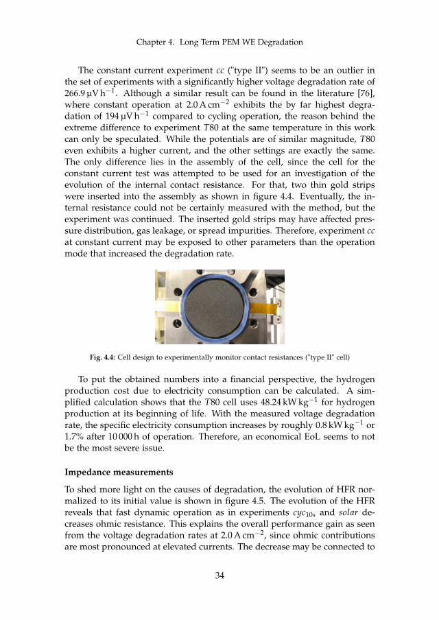
Chapter 4. Long Term PEM WE Degradation
The constant current experiment cc ("type II") seems to be an outlier inthe set of experiments with a significantly higher voltage degradation rate of266.9 µV h−1. Although a similar result can be found in the literature [76],where constant operation at 2.0 A cm−2 exhibits the by far highest degra-dation of 194 µV h−1 compared to cycling operation, the reason behind theextreme difference to experiment T80 at the same temperature in this workcan only be speculated. While the potentials are of similar magnitude, T80even exhibits a higher current, and the other settings are exactly the same.The only difference lies in the assembly of the cell, since the cell for theconstant current test was attempted to be used for an investigation of theevolution of the internal contact resistance. For that, two thin gold stripswere inserted into the assembly as shown in figure 4.4. Eventually, the in-ternal resistance could not be certainly measured with the method, but theexperiment was continued. The inserted gold strips may have affected pres-sure distribution, gas leakage, or spread impurities. Therefore, experiment ccat constant current may be exposed to other parameters than the operationmode that increased the degradation rate.
Fig. 4.4: Cell design to experimentally monitor contact resistances ("type II" cell)
To put the obtained numbers into a financial perspective, the hydrogenproduction cost due to electricity consumption can be calculated. A sim-plified calculation shows that the T80 cell uses 48.24 kW kg−1 for hydrogenproduction at its beginning of life. With the measured voltage degradationrate, the specific electricity consumption increases by roughly 0.8 kW kg−1 or1.7% after 10 000 h of operation. Therefore, an economical EoL seems to notbe the most severe issue.
Impedance measurements
To shed more light on the causes of degradation, the evolution of HFR nor-malized to its initial value is shown in figure 4.5. The evolution of the HFRreveals that fast dynamic operation as in experiments cyc10s and solar de-creases ohmic resistance. This explains the overall performance gain as seenfrom the voltage degradation rates at 2.0 A cm−2, since ohmic contributionsare most pronounced at elevated currents. The decrease may be connected to
34
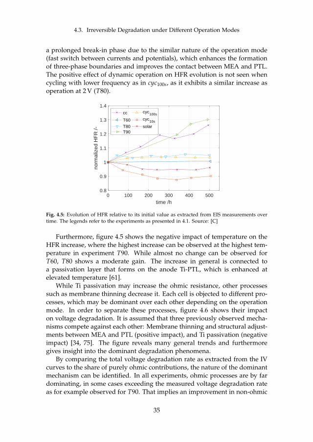
4.3. Irreversible Degradation under Different Operation Modes
a prolonged break-in phase due to the similar nature of the operation mode(fast switch between currents and potentials), which enhances the formationof three-phase boundaries and improves the contact between MEA and PTL.The positive effect of dynamic operation on HFR evolution is not seen whencycling with lower frequency as in cyc100s, as it exhibits a similar increase asoperation at 2 V (T80).
0 100 200 300 400 500
time /h
0.8
0.9
1
1.1
1.2
1.3
1.4
norm
aliz
ed H
FR
/-
cc
T60
T80T90
cyc100s
cyc10s
solar
Fig. 4.5: Evolution of HFR relative to its initial value as extracted from EIS measurements overtime. The legends refer to the experiments as presented in 4.1. Source: [C]
Furthermore, figure 4.5 shows the negative impact of temperature on theHFR increase, where the highest increase can be observed at the highest tem-perature in experiment T90. While almost no change can be observed forT60, T80 shows a moderate gain. The increase in general is connected toa passivation layer that forms on the anode Ti-PTL, which is enhanced atelevated temperature [61].
While Ti passivation may increase the ohmic resistance, other processessuch as membrane thinning decrease it. Each cell is objected to different pro-cesses, which may be dominant over each other depending on the operationmode. In order to separate these processes, figure 4.6 shows their impacton voltage degradation. It is assumed that three previously observed mecha-nisms compete against each other: Membrane thinning and structural adjust-ments between MEA and PTL (positive impact), and Ti passivation (negativeimpact) [34, 75]. The figure reveals many general trends and furthermoregives insight into the dominant degradation phenomena.
By comparing the total voltage degradation rate as extracted from the IVcurves to the share of purely ohmic contributions, the nature of the dominantmechanism can be identified. In all experiments, ohmic processes are by fardominating, in some cases exceeding the measured voltage degradation rateas for example observed for T90. That implies an improvement in non-ohmic
35
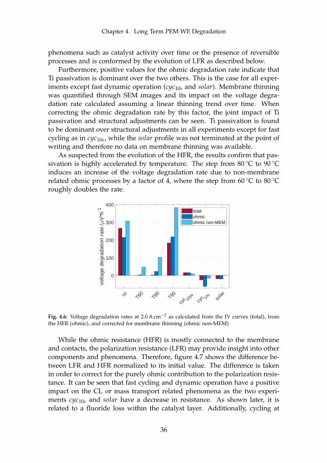
Chapter 4. Long Term PEM WE Degradation
phenomena such as catalyst activity over time or the presence of reversibleprocesses and is conformed by the evolution of LFR as described below.
Furthermore, positive values for the ohmic degradation rate indicate thatTi passivation is dominant over the two others. This is the case for all exper-iments except fast dynamic operation (cyc10s and solar). Membrane thinningwas quantified through SEM images and its impact on the voltage degra-dation rate calculated assuming a linear thinning trend over time. Whencorrecting the ohmic degradation rate by this factor, the joint impact of Tipassivation and structural adjustments can be seen. Ti passivation is foundto be dominant over structural adjustments in all experiments except for fastcycling as in cyc10s, while the solar profile was not terminated at the point ofwriting and therefore no data on membrane thinning was available.
As suspected from the evolution of the HFR, the results confirm that pas-sivation is highly accelerated by temperature. The step from 80 C to 90 Cinduces an increase of the voltage degradation rate due to non-membranerelated ohmic processes by a factor of 4, where the step from 60 C to 80 Croughly doubles the rate.
cc T60 T80 T90
cyc 10
0s
cyc 10
sso
lar
0
100
200
300
400
volta
ge d
egra
datio
n ra
te /
V*h
-1 totalohmicohmic non-MEM
Fig. 4.6: Voltage degradation rates at 2.0 A cm−2 as calculated from the IV curves (total), fromthe HFR (ohmic), and corrected for membrane thinning (ohmic non-MEM)
While the ohmic resistance (HFR) is mostly connected to the membraneand contacts, the polarization resistance (LFR) may provide insight into othercomponents and phenomena. Therefore, figure 4.7 shows the difference be-tween LFR and HFR normalized to its initial value. The difference is takenin order to correct for the purely ohmic contribution to the polarization resis-tance. It can be seen that fast cycling and dynamic operation have a positiveimpact on the CL or mass transport related phenomena as the two experi-ments cyc10s and solar have a decrease in resistance. As shown later, it isrelated to a fluoride loss within the catalyst layer. Additionally, cycling at
36
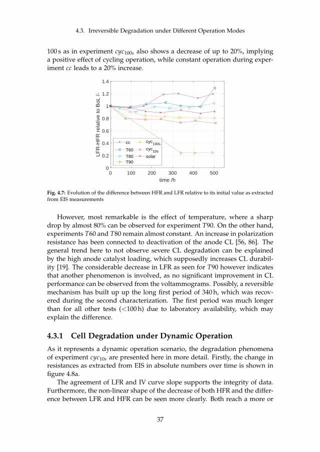
4.3. Irreversible Degradation under Different Operation Modes
100 s as in experiment cyc100s also shows a decrease of up to 20%, implyinga positive effect of cycling operation, while constant operation during exper-iment cc leads to a 20% increase.
0 100 200 300 400 500
time /h
0
0.2
0.4
0.6
0.8
1
1.2
1.4
LFR
-HF
R r
elat
ive
to B
oL /-
cc
T60
T80T90
cyc100s
cyc10s
solar
Fig. 4.7: Evolution of the difference between HFR and LFR relative to its initial value as extractedfrom EIS measurements
However, most remarkable is the effect of temperature, where a sharpdrop by almost 80% can be observed for experiment T90. On the other hand,experiments T60 and T80 remain almost constant. An increase in polarizationresistance has been connected to deactivation of the anode CL [56, 86]. Thegeneral trend here to not observe severe CL degradation can be explainedby the high anode catalyst loading, which supposedly increases CL durabil-ity [19]. The considerable decrease in LFR as seen for T90 however indicatesthat another phenomenon is involved, as no significant improvement in CLperformance can be observed from the voltammograms. Possibly, a reversiblemechanism has built up up the long first period of 340 h, which was recov-ered during the second characterization. The first period was much longerthan for all other tests (<100 h) due to laboratory availability, which mayexplain the difference.
4.3.1 Cell Degradation under Dynamic Operation
As it represents a dynamic operation scenario, the degradation phenomenaof experiment cyc10s are presented here in more detail. Firstly, the change inresistances as extracted from EIS in absolute numbers over time is shown infigure 4.8a.
The agreement of LFR and IV curve slope supports the integrity of data.Furthermore, the non-linear shape of the decrease of both HFR and the differ-ence between LFR and HFR can be seen more clearly. Both reach a more or
37
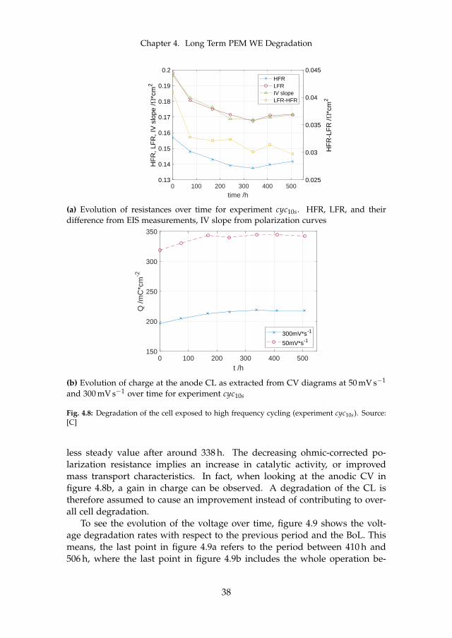
Chapter 4. Long Term PEM WE Degradation
0 100 200 300 400 500
time /h
0.13
0.14
0.15
0.16
0.17
0.18
0.19
0.2
HF
R, L
FR
, IV
slo
pe /
*cm
2
0.025
0.03
0.035
0.04
0.045
HF
R-L
FR
/*c
m2
HFRLFRIV slopeLFR-HFR
(a) Evolution of resistances over time for experiment cyc10s. HFR, LFR, and theirdifference from EIS measurements, IV slope from polarization curves
0 100 200 300 400 500
t /h
150
200
250
300
350
Q /m
C*c
m-2
300mV*s-1
50mV*s-1
(b) Evolution of charge at the anode CL as extracted from CV diagrams at 50 mV s−1
and 300 mV s−1 over time for experiment cyc10s
Fig. 4.8: Degradation of the cell exposed to high frequency cycling (experiment cyc10s). Source:[C]
less steady value after around 338 h. The decreasing ohmic-corrected po-larization resistance implies an increase in catalytic activity, or improvedmass transport characteristics. In fact, when looking at the anodic CV infigure 4.8b, a gain in charge can be observed. A degradation of the CL istherefore assumed to cause an improvement instead of contributing to over-all cell degradation.
To see the evolution of the voltage over time, figure 4.9 shows the volt-age degradation rates with respect to the previous period and the BoL. Thismeans, the last point in figure 4.9a refers to the period between 410 h and506 h, where the last point in figure 4.9b includes the whole operation be-
38

4.3. Irreversible Degradation under Different Operation Modes
tween 0 h and 506 h. It can be seen, that the performance at a current den-sity of 2.0 A cm−2 increases until 338 h, after which it decreases, while lowercurrents of <1 A cm−2 experience a decrease in performance throughout thewhole experiment. This is in line with the previously described decrease ofHFR, which is connected to the ohmic overpotential and therefore more pro-nounced at higher currents. Also the non-linear shape of the change in HFRover time can be found when looking at figure 4.9b. The data suggests thatthe dominant degradation mechanism for this operation mode changes frombeing adjustments within the CL and membrane thinning, to Ti passivation ataround 338 h. However, the overall change in performance after 500 h is stillpositive. Finally, the steady voltage degradation of around 50 µV h−1 at cur-rent densities <0.5 A cm−2 indicates that thermodynamic processes degradeconstantly.
0 100 200 300 400 500 600
time /h
-250
-200
-150
-100
-50
0
50
100
volta
ge d
egra
datio
n ra
te /
V*h
-1
0.1 A*cm-2
0.5 A*cm-2
1.0 A*cm-2
2.0 A*cm-2
(a) voltage degradation rates relativeto the last period
0 100 200 300 400 500
time /h
-250
-200
-150
-100
-50
0
50
100vo
ltage
deg
rada
tion
rate
/V
*h-1
0.1 A*cm-2
0.5 A*cm-2
1.0 A*cm-2
2.0 A*cm-2
(b) voltage degradation rates relativeto the beginning of life. Source: [C]
Fig. 4.9: Evolution of voltage degradation rates at various current densities over time for fastcycling operation (experiment cyc10s)
39

Chapter 4. Long Term PEM WE Degradation
40
Chapter 5
Membrane DegradationThrough Fluoride Emission
With respect to the research objective to develop a lifetime model, this chaptersummarizes the work on membrane degradation. Although all componentsmay degrade over time, irreversible membrane thinning through radical at-tack is the most severe mechanism and has been identified to be lifetimelimiting [32]. The major issue is an increased gas crossover due to a lowerthickness, which may create hazardous gas mixtures within the explosionlimits. The outcomes are published in [C], [D], and [C2] (see thesis outline).
5.1 Experimental Investigation on Fluoride Emis-sion
State of the art ionomers for PEM WE membranes are based on perfluoro-sulfonic acid (PFSA) and are for example known under the brand namesNafion® (DuPont) or Aquivion® (Solvay). Commonly, one of their maincomponents is fluorine (F). Except for the binder within the catalyst layers,fluorine can usually not be found in other components of a PEM WE cell.Therefore, traces of fluoride (the negatively charged ion of fluorine) leavingthe cell outlets are an indication of ionomer degradation. This approach iswidely applied within PEM FC research [49, 60] and can also be observed forPEM WE [34, 59].
In this experiment, the fluoride concentration within the effluent water atthe anode and cathode outlets was monitored over time for all seven experi-ments on "type II" cells as shown in table 4.1. On average, the anode showedless than 40% of the fluoride emission at the cathode, which is in line withprevious findings in the literature [34]. The FER at the cathode outlet for all
41
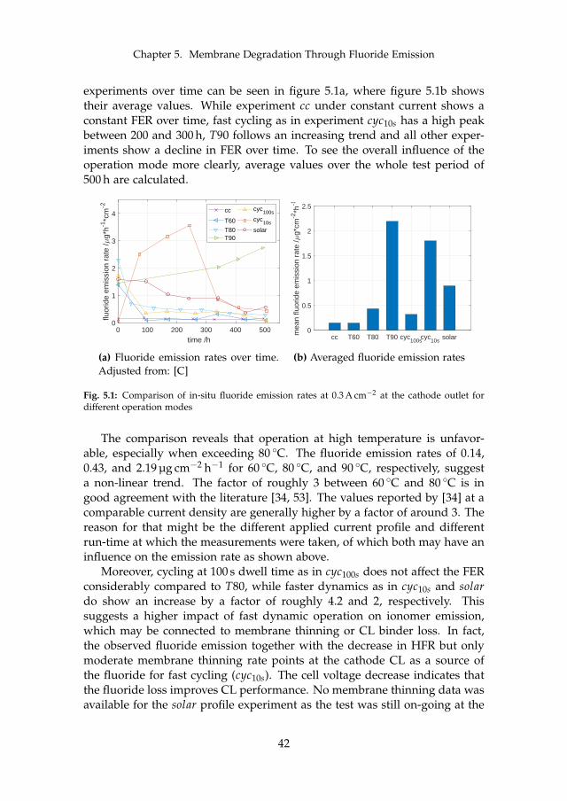
Chapter 5. Membrane Degradation Through Fluoride Emission
experiments over time can be seen in figure 5.1a, where figure 5.1b showstheir average values. While experiment cc under constant current shows aconstant FER over time, fast cycling as in experiment cyc10s has a high peakbetween 200 and 300 h, T90 follows an increasing trend and all other exper-iments show a decline in FER over time. To see the overall influence of theoperation mode more clearly, average values over the whole test period of500 h are calculated.
0 100 200 300 400 500
time /h
0
1
2
3
4
fluor
ide
emis
sion
rat
e /
g*h-1
*cm
-2
cc
T60
T80T90
cyc100s
cyc10s
solar
(a) Fluoride emission rates over time.Adjusted from: [C]
cc T60 T80 T90 cyc100s
cyc10s solar
0
0.5
1
1.5
2
2.5
mea
n flu
orid
e em
issi
on r
ate
/g*
cm-2
*h-1
(b) Averaged fluoride emission rates
Fig. 5.1: Comparison of in-situ fluoride emission rates at 0.3 A cm−2 at the cathode outlet fordifferent operation modes
The comparison reveals that operation at high temperature is unfavor-able, especially when exceeding 80 C. The fluoride emission rates of 0.14,0.43, and 2.19 µg cm−2 h−1 for 60 C, 80 C, and 90 C, respectively, suggesta non-linear trend. The factor of roughly 3 between 60 C and 80 C is ingood agreement with the literature [34, 53]. The values reported by [34] at acomparable current density are generally higher by a factor of around 3. Thereason for that might be the different applied current profile and differentrun-time at which the measurements were taken, of which both may have aninfluence on the emission rate as shown above.
Moreover, cycling at 100 s dwell time as in cyc100s does not affect the FERconsiderably compared to T80, while faster dynamics as in cyc10s and solardo show an increase by a factor of roughly 4.2 and 2, respectively. Thissuggests a higher impact of fast dynamic operation on ionomer emission,which may be connected to membrane thinning or CL binder loss. In fact,the observed fluoride emission together with the decrease in HFR but onlymoderate membrane thinning rate points at the cathode CL as a source ofthe fluoride for fast cycling (cyc10s). The cell voltage decrease indicates thatthe fluoride loss improves CL performance. No membrane thinning data wasavailable for the solar profile experiment as the test was still on-going at the
42
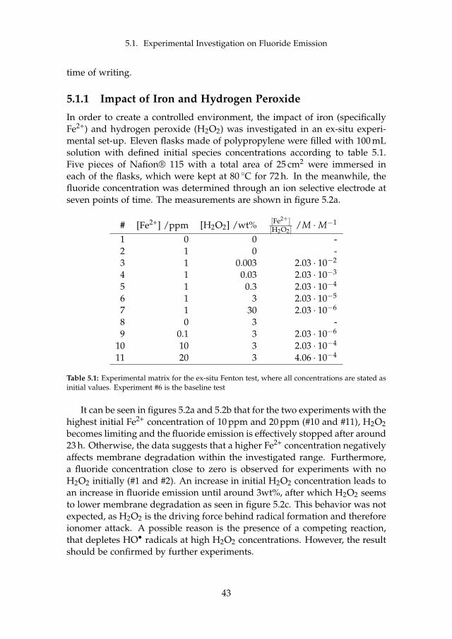
5.1. Experimental Investigation on Fluoride Emission
time of writing.
5.1.1 Impact of Iron and Hydrogen Peroxide
In order to create a controlled environment, the impact of iron (specificallyFe2+) and hydrogen peroxide (H2O2) was investigated in an ex-situ experi-mental set-up. Eleven flasks made of polypropylene were filled with 100 mLsolution with defined initial species concentrations according to table 5.1.Five pieces of Nafion® 115 with a total area of 25 cm2 were immersed ineach of the flasks, which were kept at 80 C for 72 h. In the meanwhile, thefluoride concentration was determined through an ion selective electrode atseven points of time. The measurements are shown in figure 5.2a.
# [Fe2+] /ppm [H2O2] /wt% [Fe2+ ][H2O2]
/M ·M−1
1 0 0 -2 1 0 -3 1 0.003 2.03 · 10−2
4 1 0.03 2.03 · 10−3
5 1 0.3 2.03 · 10−4
6 1 3 2.03 · 10−5
7 1 30 2.03 · 10−6
8 0 3 -9 0.1 3 2.03 · 10−6
10 10 3 2.03 · 10−4
11 20 3 4.06 · 10−4
Table 5.1: Experimental matrix for the ex-situ Fenton test, where all concentrations are stated asinitial values. Experiment #6 is the baseline test
It can be seen in figures 5.2a and 5.2b that for the two experiments with thehighest initial Fe2+ concentration of 10 ppm and 20 ppm (#10 and #11), H2O2becomes limiting and the fluoride emission is effectively stopped after around23 h. Otherwise, the data suggests that a higher Fe2+ concentration negativelyaffects membrane degradation within the investigated range. Furthermore,a fluoride concentration close to zero is observed for experiments with noH2O2 initially (#1 and #2). An increase in initial H2O2 concentration leads toan increase in fluoride emission until around 3wt%, after which H2O2 seemsto lower membrane degradation as seen in figure 5.2c. This behavior was notexpected, as H2O2 is the driving force behind radical formation and thereforeionomer attack. A possible reason is the presence of a competing reaction,that depletes HO• radicals at high H2O2 concentrations. However, the resultshould be confirmed by further experiments.
43
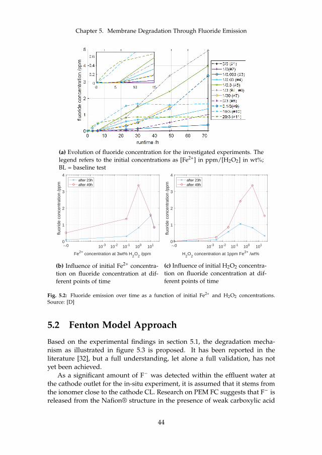
Chapter 5. Membrane Degradation Through Fluoride Emission
(a) Evolution of fluoride concentration for the investigated experiments. Thelegend refers to the initial concentrations as [Fe2+] in ppm/[H2O2] in wt%;BL = baseline test
0 10-3 10-2 10-1 100 101
Fe2+ concentration at 3wt% H2O
2 /ppm
0
1
2
3
4
fluor
ide
conc
entr
atio
n /p
pm
after 23hafter 49h
(b) Influence of initial Fe2+ concentra-tion on fluoride concentration at dif-ferent points of time
0 10-3 10-2 10-1 100 101
H2O
2 concentration at 1ppm Fe2+ /wt%
0
1
2
3
4
fluor
ide
conc
entr
atio
n /p
pm
after 23hafter 49h
(c) Influence of initial H2O2 concentra-tion on fluoride concentration at dif-ferent points of time
Fig. 5.2: Fluoride emission over time as a function of initial Fe2+ and H2O2 concentrations.Source: [D]
5.2 Fenton Model Approach
Based on the experimental findings in section 5.1, the degradation mecha-nism as illustrated in figure 5.3 is proposed. It has been reported in theliterature [32], but a full understanding, let alone a full validation, has notyet been achieved.
As a significant amount of F– was detected within the effluent water atthe cathode outlet for the in-situ experiment, it is assumed that it stems fromthe ionomer close to the cathode CL. Research on PEM FC suggests that F– isreleased from the Nafion® structure in the presence of weak carboxylic acid
44
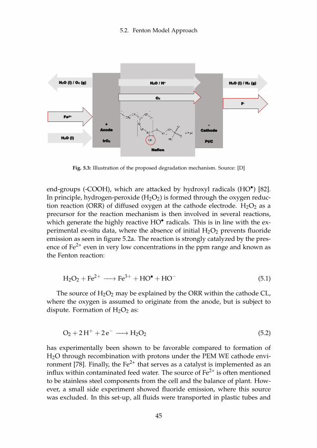
5.2. Fenton Model Approach
Nafion
-
Cathode
Pt/C
+
Anode
IrO2 H2O (l)
H2O (l) / O2 (g) H2O (l) / H2 (g) H2O / H+
O2
Fe2+
F-
Fig. 5.3: Illustration of the proposed degradation mechanism. Source: [D]
end-groups (-COOH), which are attacked by hydroxyl radicals (HO•) [82].In principle, hydrogen-peroxide (H2O2) is formed through the oxygen reduc-tion reaction (ORR) of diffused oxygen at the cathode electrode. H2O2 as aprecursor for the reaction mechanism is then involved in several reactions,which generate the highly reactive HO• radicals. This is in line with the ex-perimental ex-situ data, where the absence of initial H2O2 prevents fluorideemission as seen in figure 5.2a. The reaction is strongly catalyzed by the pres-ence of Fe2+ even in very low concentrations in the ppm range and known asthe Fenton reaction:
H2O2 + Fe2+ −−→ Fe3+ + HO• + HO− (5.1)
The source of H2O2 may be explained by the ORR within the cathode CL,where the oxygen is assumed to originate from the anode, but is subject todispute. Formation of H2O2 as:
O2 + 2 H+ + 2 e− −−→ H2O2 (5.2)
has experimentally been shown to be favorable compared to formation ofH2O through recombination with protons under the PEM WE cathode envi-ronment [78]. Finally, the Fe2+ that serves as a catalyst is implemented as aninflux within contaminated feed water. The source of Fe2+ is often mentionedto be stainless steel components from the cell and the balance of plant. How-ever, a small side experiment showed fluoride emission, where this sourcewas excluded. In this set-up, all fluids were transported in plastic tubes and
45
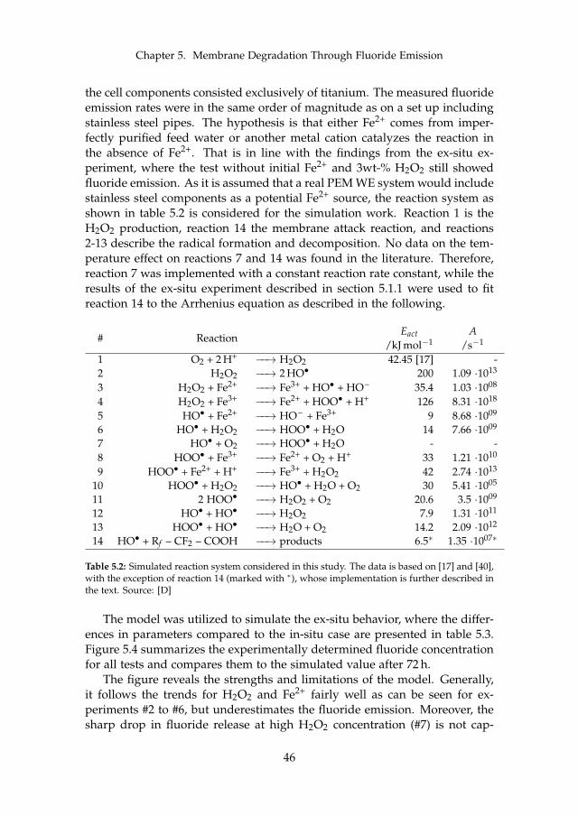
Chapter 5. Membrane Degradation Through Fluoride Emission
the cell components consisted exclusively of titanium. The measured fluorideemission rates were in the same order of magnitude as on a set up includingstainless steel pipes. The hypothesis is that either Fe2+ comes from imper-fectly purified feed water or another metal cation catalyzes the reaction inthe absence of Fe2+. That is in line with the findings from the ex-situ ex-periment, where the test without initial Fe2+ and 3wt-% H2O2 still showedfluoride emission. As it is assumed that a real PEM WE system would includestainless steel components as a potential Fe2+ source, the reaction system asshown in table 5.2 is considered for the simulation work. Reaction 1 is theH2O2 production, reaction 14 the membrane attack reaction, and reactions2-13 describe the radical formation and decomposition. No data on the tem-perature effect on reactions 7 and 14 was found in the literature. Therefore,reaction 7 was implemented with a constant reaction rate constant, while theresults of the ex-situ experiment described in section 5.1.1 were used to fitreaction 14 to the Arrhenius equation as described in the following.
# ReactionEact
/kJ mol−1A
/s−1
1 O2 + 2 H+ −−→ H2O2 42.45 [17] -2 H2O2 −−→ 2 HO• 200 1.09 ·1013
3 H2O2 + Fe2+ −−→ Fe3+ + HO• + HO– 35.4 1.03 ·1008
4 H2O2 + Fe3+ −−→ Fe2+ + HOO• + H+ 126 8.31 ·1018
5 HO• + Fe2+ −−→ HO– + Fe3+ 9 8.68 ·1009
6 HO• + H2O2 −−→ HOO• + H2O 14 7.66 ·1009
7 HO• + O2 −−→ HOO• + H2O - -8 HOO• + Fe3+ −−→ Fe2+ + O2 + H+ 33 1.21 ·1010
9 HOO• + Fe2+ + H+ −−→ Fe3+ + H2O2 42 2.74 ·1013
10 HOO• + H2O2 −−→ HO• + H2O + O2 30 5.41 ·1005
11 2 HOO• −−→ H2O2 + O2 20.6 3.5 ·1009
12 HO• + HO• −−→ H2O2 7.9 1.31 ·1011
13 HOO• + HO• −−→ H2O + O2 14.2 2.09 ·1012
14 HO• + Rf – CF2 – COOH −−→ products 6.5∗ 1.35 ·1007∗
Table 5.2: Simulated reaction system considered in this study. The data is based on [17] and [40],with the exception of reaction 14 (marked with ∗), whose implementation is further described inthe text. Source: [D]
The model was utilized to simulate the ex-situ behavior, where the differ-ences in parameters compared to the in-situ case are presented in table 5.3.Figure 5.4 summarizes the experimentally determined fluoride concentrationfor all tests and compares them to the simulated value after 72 h.
The figure reveals the strengths and limitations of the model. Generally,it follows the trends for H2O2 and Fe2+ fairly well as can be seen for ex-periments #2 to #6, but underestimates the fluoride emission. Moreover, thesharp drop in fluoride release at high H2O2 concentration (#7) is not cap-
46
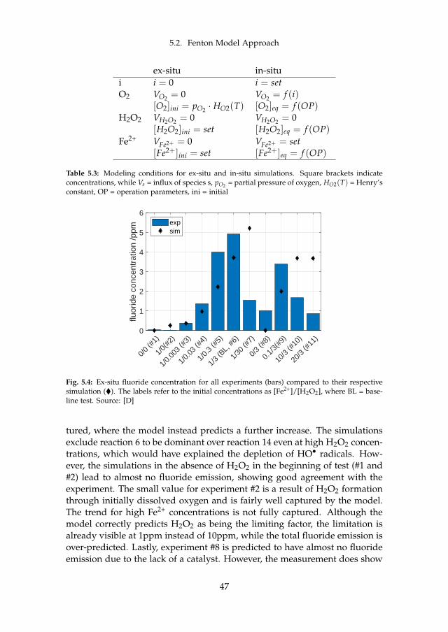
5.2. Fenton Model Approach
ex-situ in-situi i = 0 i = setO2 VO2 = 0 VO2 = f (i)
[O2]ini = pO2 · HO2(T) [O2]eq = f (OP)H2O2 VH2O2 = 0 VH2O2 = 0
[H2O2]ini = set [H2O2]eq = f (OP)Fe2+ VFe2+ = 0 VFe2+ = set
[Fe2+]ini = set [Fe2+]eq = f (OP)
Table 5.3: Modeling conditions for ex-situ and in-situ simulations. Square brackets indicateconcentrations, while Vs = influx of species s, pO2 = partial pressure of oxygen, HO2(T) = Henry’sconstant, OP = operation parameters, ini = initial
0/0
(#1)
1/0(
#2)
1/0.
003
(#3)
1/0.
03 (#
4)
1/0.
3 (#
5)
1/3
(BL,
#6)
1/30
(#7)
0/3
(#8)
0.1/
3(#9
)
10/3
(#10
)
20/3
(#11
)0
1
2
3
4
5
6
fluor
ide
conc
entr
atio
n /p
pm
expsim
Fig. 5.4: Ex-situ fluoride concentration for all experiments (bars) compared to their respectivesimulation (). The labels refer to the initial concentrations as [Fe2+]/[H2O2], where BL = base-line test. Source: [D]
tured, where the model instead predicts a further increase. The simulationsexclude reaction 6 to be dominant over reaction 14 even at high H2O2 concen-trations, which would have explained the depletion of HO• radicals. How-ever, the simulations in the absence of H2O2 in the beginning of test (#1 and#2) lead to almost no fluoride emission, showing good agreement with theexperiment. The small value for experiment #2 is a result of H2O2 formationthrough initially dissolved oxygen and is fairly well captured by the model.The trend for high Fe2+ concentrations is not fully captured. Although themodel correctly predicts H2O2 as being the limiting factor, the limitation isalready visible at 1ppm instead of 10ppm, while the total fluoride emission isover-predicted. Lastly, experiment #8 is predicted to have almost no fluorideemission due to the lack of a catalyst. However, the measurement does show
47
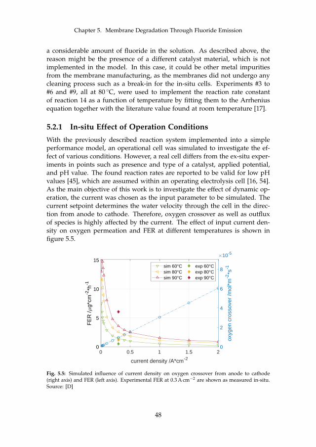
Chapter 5. Membrane Degradation Through Fluoride Emission
a considerable amount of fluoride in the solution. As described above, thereason might be the presence of a different catalyst material, which is notimplemented in the model. In this case, it could be other metal impuritiesfrom the membrane manufacturing, as the membranes did not undergo anycleaning process such as a break-in for the in-situ cells. Experiments #3 to#6 and #9, all at 80 C, were used to implement the reaction rate constantof reaction 14 as a function of temperature by fitting them to the Arrheniusequation together with the literature value found at room temperature [17].
5.2.1 In-situ Effect of Operation Conditions
With the previously described reaction system implemented into a simpleperformance model, an operational cell was simulated to investigate the ef-fect of various conditions. However, a real cell differs from the ex-situ exper-iments in points such as presence and type of a catalyst, applied potential,and pH value. The found reaction rates are reported to be valid for low pHvalues [45], which are assumed within an operating electrolysis cell [16, 54].As the main objective of this work is to investigate the effect of dynamic op-eration, the current was chosen as the input parameter to be simulated. Thecurrent setpoint determines the water velocity through the cell in the direc-tion from anode to cathode. Therefore, oxygen crossover as well as outfluxof species is highly affected by the current. The effect of input current den-sity on oxygen permeation and FER at different temperatures is shown infigure 5.5.
0 0.5 1 1.5 2
current density /A*cm-2
0
5
10
15
FE
R /
g*cm
-2*h
-1
0
2
4
6
8
oxyg
en c
ross
over
/mol
*m-2
*s-1
10-5
sim 60°Csim 80°Csim 90°C
exp 60°Cexp 80°Cexp 90°C
Fig. 5.5: Simulated influence of current density on oxygen crossover from anode to cathode(right axis) and FER (left axis). Experimental FER at 0.3 A cm−2 are shown as measured in-situ.Source: [D]
48
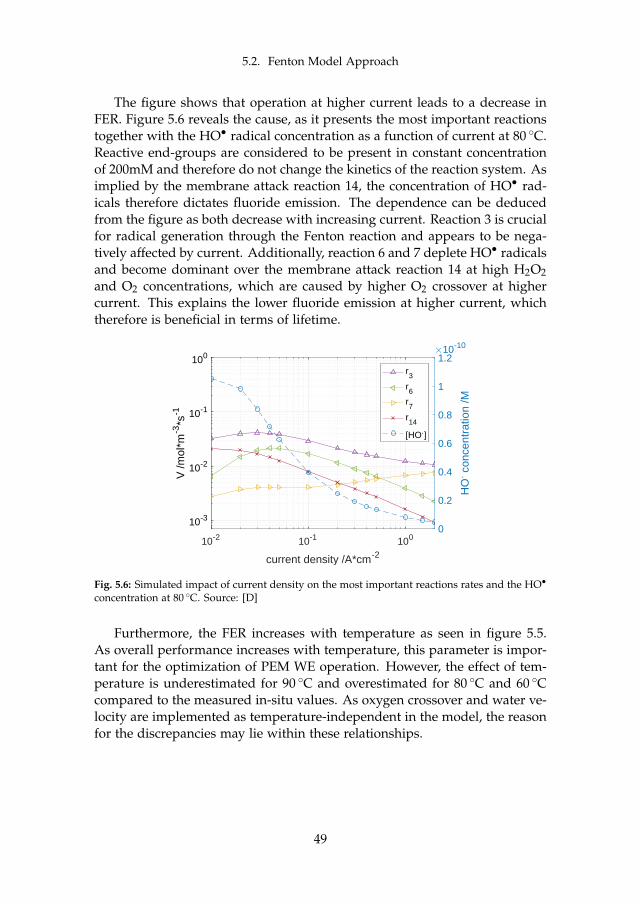
5.2. Fenton Model Approach
The figure shows that operation at higher current leads to a decrease inFER. Figure 5.6 reveals the cause, as it presents the most important reactionstogether with the HO• radical concentration as a function of current at 80 C.Reactive end-groups are considered to be present in constant concentrationof 200mM and therefore do not change the kinetics of the reaction system. Asimplied by the membrane attack reaction 14, the concentration of HO• rad-icals therefore dictates fluoride emission. The dependence can be deducedfrom the figure as both decrease with increasing current. Reaction 3 is crucialfor radical generation through the Fenton reaction and appears to be nega-tively affected by current. Additionally, reaction 6 and 7 deplete HO• radicalsand become dominant over the membrane attack reaction 14 at high H2O2and O2 concentrations, which are caused by higher O2 crossover at highercurrent. This explains the lower fluoride emission at higher current, whichtherefore is beneficial in terms of lifetime.
10-2 10-1 100
current density /A*cm-2
10-3
10-2
10-1
100
V /m
ol*m
-3*s
-1
0
0.2
0.4
0.6
0.8
1
1.2
HO
. con
cent
ratio
n /M
10-10
r3
r6
r7
r14
[HO.]
Fig. 5.6: Simulated impact of current density on the most important reactions rates and the HO•
concentration at 80 C. Source: [D]
Furthermore, the FER increases with temperature as seen in figure 5.5.As overall performance increases with temperature, this parameter is impor-tant for the optimization of PEM WE operation. However, the effect of tem-perature is underestimated for 90 C and overestimated for 80 C and 60 Ccompared to the measured in-situ values. As oxygen crossover and water ve-locity are implemented as temperature-independent in the model, the reasonfor the discrepancies may lie within these relationships.
49
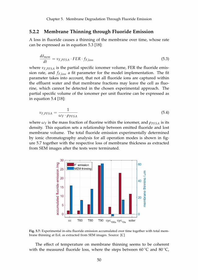
Chapter 5. Membrane Degradation Through Fluoride Emission
5.2.2 Membrane Thinning through Fluoride Emission
A loss in fluoride causes a thinning of the membrane over time, whose ratecan be expressed as in equation 5.3 [18]:
dδmem
dt= νF,PFSA · FER · fF,loss (5.3)
where νF,PFSA is the partial specific ionomer volume, FER the fluoride emis-sion rate, and fF,loss a fit parameter for the model implementation. The fitparameter takes into account, that not all fluoride ions are captured withinthe effluent water and that membrane fractions may leave the cell as fluo-rine, which cannot be detected in the chosen experimental approach. Thepartial specific volume of the ionomer per unit fluorine can be expressed asin equation 5.4 [18]:
νF,PFSA =1
ωF · ρPFSA(5.4)
where ωF is the mass fraction of fluorine within the ionomer, and ρPFSA is itsdensity. This equation sets a relationship between emitted fluoride and lostmembrane volume. The total fluoride emission experimentally determinedby ionic chromatography analysis for all operation modes is shown in fig-ure 5.7 together with the respective loss of membrane thickness as extractedfrom SEM images after the tests were terminated.
Fig. 5.7: Experimental in-situ fluoride emission accumulated over time together with total mem-brane thinning at EoL as extracted from SEM images. Source: [C]
The effect of temperature on membrane thinning seems to be coherentwith the measured fluoride loss, where the steps between 60 C and 80 C,
50
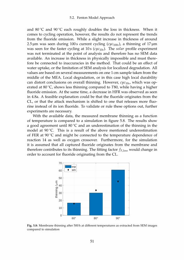
5.2. Fenton Model Approach
and 80 C and 90 C each roughly doubles the loss in thickness. When itcomes to cycling operation, however, the results do not represent the trendsfrom the fluoride emission. While a slight increase in thickness of around2.5 µm was seen during 100 s current cycling (cyc100s), a thinning of 17 µmwas seen for the faster cycling at 10 s (cyc10s). The solar profile experimentwas not terminated at the point of analysis and therefore has no SEM dataavailable. An increase in thickness in physically impossible and must there-fore be connected to inaccuracies in the method. That could be an effect ofwater uptake, or the limitation of SEM analysis for localized degradation. Allvalues are based on several measurements on one 1 cm sample taken from themiddle of the MEA. Local degradation, or in this case high local durabilitycan distort conclusions on overall thinning. However, cyc10s, which was op-erated at 80 C, shows less thinning compared to T80, while having a higherfluoride emission. At the same time, a decrease in HFR was observed as seenin 4.8a. A feasible explanation could be that the fluoride originates from theCL, or that the attack mechanism is shifted to one that releases more fluo-rine instead of its ion fluoride. To validate or rule these options out, furtherexperiments are necessary.
With the available data, the measured membrane thinning as a functionof temperature is compared to a simulation in figure 5.8. The results showa good agreement until 80 C and an underestimation of the thinning in themodel at 90 C. This is a result of the above mentioned underestimationof FER at 90 C and might be connected to the temperature dependence ofreaction 14 as well as oxygen crossover. Furthermore, for the simulationit is assumed that all captured fluoride originates from the membrane andtherefore contributes to its thinning. The fitting factor fF,loss would change inorder to account for fluoride originating from the CL.
60° 80° 90°0
10
20
30
40
50
60
70
thin
ning
/m
expsim
Fig. 5.8: Membrane thinning after 500 h at different temperatures as extracted from SEM imagescompared to simulation
51

Chapter 5. Membrane Degradation Through Fluoride Emission
52

Chapter 6
Final Remarks
In this project, PEM WE was investigated with special focus on its degrada-tion under dynamic operation. An experimental approach combined withnumerical modeling was followed with a focus on single cells to obtain a bet-ter understanding of different degradation mechanisms. This chapter firstlysummarizes the main outcomes and contributions of this work according tothe defined objectives of the project, and secondly presents a future perspec-tive on the topic.
6.1 Conclusion
The impact of cell compression was investigated in-situ, ex-situ, and througha computational performance model on a 2.89 cm2 single cell. It was ex-perimentally found that high pressure operation decreases the total ohmiclosses due to improved contacts. The simulation further revealed a shareof roughly one-third to two-thirds between the contact resistances and themembrane resistance, where the current distributors have been found to beresponsible for a considerable share of the total contact resistance through anex-situ experiment. However, compared to the ohmic overpotential, the ac-tivation overpotential remains dominant throughout the whole investigatedcompression range even at elevated currents, and simulations suggest an op-timum compression of around 1.5 MPa for the maximum apparent exchangecurrent density. Furthermore, excessive compression may facilitate the for-mation of hot spots and pinholes.
Concerning degradation, long-term experiments on 25 cm2 single cells re-vealed that high temperature operation is beneficial in terms of performance,but negatively affects durability, especially at temperatures above 80 C. Thisis due to accelerated membrane thinning, which roughly doubles between60 C and 80 C, and 80 C and 90 C, respectively. Furthermore, the total
53
Chapter 6. Final Remarks
ohmic cell resistance increases over time due to titanium passivation, wherethe rate is likewise highly influenced by the temperature. To enable oper-ation above 80 C and benefit from the efficiency improvement, mitigationstrategies for both anode porous transport layer and membrane have to beimplemented. The porous transport layer may be platinum-coated, whichhas to experience a drop in cost for a commercial implementation. The mem-brane may be stabilized against chemical attack. This can be done throughadjustments in the chemical structure by reducing the amount of reactive endgroups, which represent the point of attack for hydroxyl radicals.
Economically, the measured voltage degradation rate for operation at80 C would increase the specific energy cost for hydrogen production by0.8 kW h kg−1 over 10 000 h, which corresponds to a 1.7% increase comparedto its initial value. This is considered to be within acceptable range for com-mercial products. Therefore, a technical or safety-related end of life is con-sidered more critical rather than an economical one.
It was furthermore experimentally found that interdigitated flow channelsexhibit a high reversible share of overall voltage increase. The potential causeare trapped oxygen bubbles in the inlet channels that hinder access to theactive sites. A sudden change in current and potential clears the reversiblevoltage increase, which indicates a positive effect of dynamic operation onreversible degradation.
Furthermore, irreversible voltage degradation has also been found to de-crease at dynamic operation with a dwell time of 10 s in a set-up with paral-lel flow field channels. This is mostly due to a decrease in ohmic resistancewithin the first 350 h of operation of around 12%, while constant operationshowed an increase. At the same time, fluoride emission is higher at dy-namic operation, while no significant difference for membrane thinning wasobserved. Therefore, the ionomer within the catalyst layer is suspected toexperience the fluoride loss, which improves performance due to an increasein three phase boundaries. However, when fluoride loss exceeds a certainthreshold, it is expected to reverse the positive effect into a negative one,which may affect lifetime. This could be due to a critical thinning of themembrane or the loss of binder within the catalyst layer.
Eventually, membrane thinning may cause the electrolyzer to reach its endof life due to increased gas crossover. Therefore, the membrane representsa lifetime-limiting component and its degradation was simulated through anumeric model implemented in Matlab/SIMULINK® . The model was sup-ported by ex-situ experiments, which found hydrogen peroxide to be crucialfor the membrane attack reaction, while iron ions act as a strong catalyst forthe membrane attack reaction even in low concentrations of a few ppm. Ironimpurities as well as other Fenton-active metallic impurities should thereforebe avoided in the system. The model was able to capture the trends con-nected to both hydrogen peroxide and iron ions. Simulations of in-situ oper-
54
6.2. Future Work
ation revealed a positive impact of high current on fluoride emission rate interms of degradation, which decreases by a factor of 5 from 0.2 to 2.0 A cm−2.The model is a functional tool to gain insights into the involved degradationmechanisms and may serve as a basis to optimize operation strategies.
6.1.1 Main Contributions
• It was found that voltage degradation for a state of the art cell designis acceptable at temperatures up to 80 C, while membrane thinning isthe lifetime limiting factor
• High temperature operation above 80 C is a crucial operation parame-ter that significantly enhances degradation due to membrane thinningand ohmic cell resistance increase
• The experiments revealed that constant operation should be avoided tominimize the effect of both reversible and irreversible voltage degrada-tion, while dynamic operation with current/potential changes of <60 sis beneficial for decreasing voltage degradation
• For the first time, a PEM WE model that takes into account the tempera-ture effect on reaction kinetics was reported. The model was supportedby experimental work on the impact of hydrogen peroxide and ironions on the reaction kinetics
6.2 Future Work
In order to see a wide implementation of the PEM WE technology, a costreduction is crucial. Concerning the presented work, the set of in-situ ex-periments should be validated and enriched by high current/high voltageoperation. A shift to higher operation currents would lead to a significantdrop in cost. Also the seemingly positive effect of current interruption andpotential shifts has to be confirmed and further investigated, for example bystudying a constant profile that is only interrupted for 1 s every 100 s. Even-tually, the results from the single cell experiments have to be validated on astack.
Furthermore, operation at high pressure has to be investigated in terms ofoperation safety and degradation. This is due to the need of pressurized hy-drogen for both storage and further utilization in industrial processes such asmethanol production. Internal pressurization may make external mechanicalcompression redundant and therefore reduce the cost.
Finally, the membrane degradation model has to be fully validated andthe origins of hydrogen peroxide and metallic ions have to be identified.
55
Chapter 6. Final Remarks
The latter is considered crucial, as even very low concentrations of Fenton-active metal impurities cause a severe effect on ionomer degradation. Feedwater purification is a costly process in terms of both money and energy andhas to be addressed in the future. Furthermore, a thorough study on thetemperature and current effect on oxygen permeation has to be carried out,where the results may benefit the model accuracy especially where the in-situfluoride emission rate is underestimated compared to the measured values.
In a broader sense, PEM WE may highly benefit from the emergence ofnew technologies such as 3D-printing, which may simplify prototyping andtherefore cut the development cost. Besides the positive effect of industrialscale production on the price, other fundamentally different approaches incell design may be beneficial for cost reduction. As bipolar plates are themajor contributor to the stack cost, they bear a high saving potential. Forexample, production cost may be reduced if the function of the flow channelswas taken over by the porous transport layer.
Lastly, the cost for the catalyst can drop significantly by replacing the stateof the art catalyst with non-noble options. However, the share of the catalystof the stack cost is less than 10%. Assuming around 60% of the system costfor the stack leaves little saving potential even by cutting the catalyst loadingin half. The more severe issue related to the catalyst is the limited availabilityof iridium, which is the driving force behind the efforts to reduce loadingand increase efficiency. Eventually, a functional alternative to iridium has tobe found to enable upscaling on a grid-level.
56
References
References
[1] Z. Abdin, C. J. Webb, and E. M. Gray, “Modelling and simulation of aproton exchange membrane ( PEM ) electrolyser cell,” International Journal ofHydrogen Energy, vol. 40, no. 39, pp. 13 243–13 257, 2015. [Online]. Available:http://dx.doi.org/10.1016/j.ijhydene.2015.07.129
[2] A. H. Abdol Rahim, A. S. Tijani, S. K. Kamarudin, and S. Hanapi, “An overviewof polymer electrolyte membrane electrolyzer for hydrogen production:Modeling and mass transport,” Journal of Power Sources, vol. 309, pp. 56–65, 2016.[Online]. Available: http://dx.doi.org/10.1016/j.jpowsour.2016.01.012
[3] F. Arbabi, H. Montazeri, R. Abouatallah, R. Wang, and A. Bazylak, “Three-Dimensional Computational Fluid Dynamics Modelling of Oxygen Bubble Trans-port in Polymer Electrolyte Membrane Electrolyzer Porous Transport Layers,”Journal of The Electrochemical Society, vol. 163, no. 11, pp. 3062–3069, 2016.
[4] A. S. Aricò, S. Siracusano, V. Baglio, N. V. Dijk, and L. Merlo, “Durability andDegradation Issues in PEM Electrolysis Cells and its Components DegradationMechanisms and Enhanced Stability of PEM Electrolysis Cells Using Low Cata-lyst Loadings and Novel Type of Membranes,” Electrohypem, Tech. Rep., 2016.
[5] A. S. Arico, S. Siracusano, N. Briguglio, V. Baglio, A. Di Blasi, and V. Antonucci,“Polymer electrolyte membrane water electrolysis: Status of technologies andpotential applications in combination with renewable power sources,” Journal ofApplied Electrochemistry, vol. 43, no. 2, pp. 107–118, 2013.
[6] K. E. Ayers, E. B. Anderson, C. B. Capuano, B. D. Carter, L. T. Dalton, G. Hanlon,J. Manco, and M. Niedzwiecki, “Research Advances Towards Low Cost, HighEfficiency PEM Electrolysis,” ECS Transactions, vol. 33, no. 1, pp. 3–15, 2010.
[7] U. Babic, M. Suermann, F. N. Büchi, L. Gubler, and T. J. Schmidt, “CriticalReview—Identifying Critical Gaps for Polymer Electrolyte Water ElectrolysisDevelopment,” Journal of The Electrochemical Society, vol. 164, no. 4, pp. F387–F399,2017. [Online]. Available: http://jes.ecsdl.org/lookup/doi/10.1149/2.1441704jes
[8] B. Bensmann, R. Hanke-Rauschenbach, G. Müller-Syring, M. Henel, andK. Sundmacher, “Optimal configuration and pressure levels of electrolyzer plantsin context of power-to-gas applications,” Applied Energy, vol. 167, p. 107–124,2016. [Online]. Available: http://dx.doi.org/10.1016/j.apenergy.2016.01.038
57
References
[9] B. Bensmann, R. Hanke-Rauschenbach, I. K. Peña Arias, and K. Sundmacher,“Energetic evaluation of high pressure PEM electrolyzer systems for interme-diate storage of renewable energies,” Electrochimica Acta, vol. 110, pp. 570–580,2013.
[10] M. Bernt and H. A. H. Gasteiger, “Influence of Ionomer Content in IrO2 /TiO 2 Electrodes on PEM Water Electrolyzer Performance,” Journal ofThe Electrochemical Society, vol. 163, no. 11, pp. F3179–F3189, 2016. [Online].Available: http://jes.ecsdl.org/lookup/doi/10.1149/2.0231611jes
[11] M. Bernt, A. Siebel, and H. A. Gasteiger, “Analysis of Voltage Losses in PEMWater Electrolyzers with Low Platinum Group Metal Loadings,” Journal of TheElectrochemical Society, vol. 165, no. 5, pp. F305–F314, 2018. [Online]. Available:http://jes.ecsdl.org/lookup/doi/10.1149/2.0641805jes
[12] L. Bertuccioli, A. Chan, D. Hart, F. Lehner, B. Madden, and E. Standen,“Development of Water Electrolysis in the European Union - FinalReport,” Fuel Cells and Hydrogen Joint Undertaking, Tech. Rep. Febru-ary, 2014. [Online]. Available: http://www.fch-ju.eu/sites/default/files/studyelectrolyser%7B_%7D0-Logos%7B_%7D0%7B_%7D0.pdfhttp://www.fch-ju.eu/sites/default/files/studyelectrolyser_0-Logos_0_0.pdf
[13] D. Bessarabov, H. Wang, H. Li, and N. Zhao, PEM Electrolysis for Hydrogen Pro-duction - Principles and Applications. CRC Press, 2016.
[14] BioLogic, “HCP-803 High Current Potentiostat,” 2018. [Online]. Avail-able: http://www.bio-logic.net/en/products/potentiostat-galvanostat-eis/hcp-803-high-current-potentiostatgalvanostateis/
[15] F. N. F. Büchi, M. Inaba, and T. J. T. T. J. Schmidt, Polymer Electrolyte Fuel CellDurability. Springer, 2009.
[16] M. Carmo, D. L. Fritz, J. Mergel, and D. Stolten, “A comprehensive review onPEM water electrolysis,” International Journal of Hydrogen Energy, vol. 38, no. 12,pp. 4901–4934, 2013.
[17] M. Chandesris, V. Médeau, N. Guillet, S. Chelghoum, D. Thoby, and F. Fouda-Onana, “Membrane degradation in PEM water electrolyzer: Numerical modelingand experimental evidence of the influence of temperature and current density,”International Journal of Hydrogen Energy, vol. 40, no. 3, pp. 1353–1366, 2015.
[18] M. Chandesris, R. Vincent, L. Guetaz, J.-S. Roch, D. Thoby, andM. Quinaud, “Membrane degradation in PEM fuel cells: From experimentalresults to semi-empirical degradation laws,” International Journal of HydrogenEnergy, vol. 42, no. 12, pp. 8139–8149, 2017. [Online]. Available: http://linkinghub.elsevier.com/retrieve/pii/S0360319917306249
[19] S. Cherevko, “Stability and dissolution of electrocatalysts : Building the bridgebetween model and “ real world ” systems,” Current Opinion in Electrochemistry,pp. 1–8, 2018. [Online]. Available: https://doi.org/10.1016/j.coelec.2018.03.034
[20] CIA, “The World Factbook: DENMARK,” 2018. [On-line]. Available: https://www.cia.gov/library/publications/resources/the-world-factbook/geos/da.html
58
References
[21] ——, “The World Factbook: ELECTRICITY - FROM HYDROELEC-TRIC PLANTS,” 2018. [Online]. Available: https://www.cia.gov/library/publications/resources/the-world-factbook/rankorder/2238rank.html
[22] ——, “The World Factbook: ELECTRICITY - FROM OTHER RENEW-ABLE SOURCES,” 2018. [Online]. Available: https://www.cia.gov/library/publications/resources/the-world-factbook/rankorder/2240rank.html
[23] ——, “The World Factbook: WORLD,” 2018. [Online]. Available: https://www.cia.gov/library/publications/resources/the-world-factbook/geos/xx.html
[24] Danish Governement, “Energy Strategy 2050 - From Coal, Oil and Gas to GreenEnergy,” Danish Energy Agency, no. February, 2011.
[25] F. De Bruijn, “PEMFC Lifetime and Durability: an overview,” in Workshop: En-twicklung von Lebensdauerprognosemodellen von Brennstoffzellen in realen Anwendun-gen, 2011.
[26] A. Diedrichs, M. Rastedt, F. J. Pinar, and P. Wagner, “Effect of compression on theperformance of a HT-PEM fuel cell,” Journal of Applied Electrochemistry, vol. 43,no. 11, pp. 1079–1099, 2013.
[27] DLR, “Abschlussbericht Verbundsvorhaben LastEISys,” DLR, Tech. Rep., 2016.
[28] Energinet, “Teknisk forskrift Automatisk og manuel elforbrugsaf- lastning,” En-erginet, Tech. Rep., 2014.
[29] ——, “Energinet Electricity Balance Data,” 2015. [Online]. Available:https://www.energidataservice.dk/en/dataset/electricitybalance/resource_extract/498c68e3-d248-4965-b36f-3aa738130adc?page=2&applied-filters=HourDK%7CBETWEEN%7C2015-07-09+00%3A00+AND+2015-07-11+00%3A00&sort=HourDK%2C+desc#resource-preview
[30] ENTSO-E, “ENTSO-E Objectives,” 2018. [Online]. Available: https://www.entsoe.eu/about/inside-entsoe/objectives/
[31] E. Fabbri, A. Habereder, K. Waltar, R. Kötz, and T. J. Schmidt, “Developmentsand perspectives of oxide-based catalysts for the oxygen evolution reaction,”Catalysis Science and Technology, vol. 4, no. 11, pp. 3800–3821, 2014.
[32] Q. Feng, X. Yuan, G. Liu, B. Wei, Z. Zhang, H. Li, and H. Wang, “A reviewof proton exchange membrane water electrolysis on degradation mechanismsand mitigation strategies,” Journal of Power Sources, vol. 366, pp. 33–55, 2017.[Online]. Available: http://dx.doi.org/10.1016/j.jpowsour.2017.09.006
[33] C. L. Fevre, “Gas storage in Great Britain,” Oxford Institutefor Energy Studies, Tech. Rep. January, 2013. [Online]. Avail-able: http://infrastructure.planningportal.gov.uk/wp-content/ipc/uploads/projects/EN030001/3.PostDecisionInformation/Decision/130409_EN030001_Chris_Le_Fevre_Report.pdf
[34] F. Fouda-Onana, M. Chandesris, V. Médeau, S. Chelghoum, D. Thoby, andN. Guillet, “Investigation on the degradation of MEAs for PEM water electrol-ysers part I: Effects of testing conditions on MEA performances and membraneproperties,” International Journal of Hydrogen Energy, vol. 41, pp. 16 627–16 636,2016.
59
References
[35] F. Fouda-Onana, “AST PROTOCOLS FOR PEM WATER ELECTROLYIS,” CEAGrenoble, Tech. Rep., 2016.
[36] M. W. Fowler, “DEGRADATION AND RELIABILITY ANALYSIS OF PEM FUELCELL STACKS Average Cell Voltage,” University of Waterloo, Tech. Rep., 2002.
[37] B. Frois, “Balancing the Grid with hydrogen technologies,” CEA, Tech.Rep., 2017. [Online]. Available: http://www.efcf.com/fileadmin/content/GSMpresentations/03_Frois.pdf
[38] A. S. Gago, S. A. Ansar, B. Saruhan, U. Schulz, P. Lettenmeier, N. A. Cañas,P. Gazdzicki, T. Morawietz, R. Hiesgen, J. Arnold, and K. A. Friedrich, “Pro-tective coatings on stainless steel bipolar plates for proton exchange membrane(PEM) electrolysers,” Journal of Power Sources, vol. 307, p. in press, 2015.
[39] Gamry Instruments, “Reference 30k Booster,” 2018. [Online]. Available:https://www.gamry.com/potentiostats/reference-30k-booster/
[40] M. Ghelichi, P. E. A. Melchy, and M. H. Eikerling, “Radically coarse-grainedapproach to the modeling of chemical degradation in fuel cell ionomers,” Journalof Physical Chemistry B, vol. 118, no. 38, pp. 11 375–11 386, 2014.
[41] S. A. Grigoriev, K. Dzhus, D. G. Bessarabov, and P. Millet, “Failure ofPEM water electrolysis cells: Case study involving anode dissolution andmembrane thinning,” International Journal of Hydrogen Energy, vol. 39, no. 35,pp. 1–7, 2014. [Online]. Available: http://linkinghub.elsevier.com/retrieve/pii/S0360319914013913
[42] S. A. Grigoriev, A. A. Kalinnikov, P. Millet, V. I. Porembsky, and V. N. Fateev,“Mathematical modeling of high-pressure PEM water electrolysis,” Journal of Ap-plied Electrochemistry, vol. 40, no. 5, pp. 921–932, 2010.
[43] S. A. Grigoriev, P. Millet, S. V. Korobtsev, V. I. Porembskiy, M. Pepic,C. Etievant, C. Puyenchet, and V. N. Fateev, “Hydrogen safety aspects relatedto high-pressure polymer electrolyte membrane water electrolysis,” InternationalJournal of Hydrogen Energy, vol. 34, no. 14, pp. 5986–5991, 2009. [Online].Available: http://dx.doi.org/10.1016/j.ijhydene.2009.01.047
[44] S. A. Grigoriev, V. I. Porembskiy, S. V. Korobtsev, V. N. Fateev, F. Aupre, andP. Millet, “High-pressure PEM water electrolysis and corresponding safety is-sues,” International Journal of Hydrogen Energy, vol. 6, pp. 3–10, 2010.
[45] L. Gubler, S. M. Dockheer, and W. H. Koppenol, “Radical (HO, H and HOO)Formation and Ionomer Degradation in Polymer Electrolyte Fuel Cells,” Journalof The Electrochemical Society, vol. 158, no. 7, p. B755, 2011. [Online]. Available:http://jes.ecsdl.org/cgi/doi/10.1149/1.3581040
[46] F. Gutiérrez-Martín and I. Guerrero-Hernández, “Balancing the grid loads bylarge scale integration of hydrogen technologies: The case of the Spanish powersystem,” International Journal of Hydrogen Energy, vol. 37, no. 2, pp. 1151–1161,2012.
[47] A. W. Hofmann, Introduction to modern chemistry experimental and theoretical.WALTON AND MABERLY, London, 1866.
60
References
[48] IEA International Energy Agency, “Key World Energy statistics,” 2017. [Online].Available: http://www.enecho.meti.go.jp/statistics/total_energy/results.html
[49] M. Inaba, T. Kinumoto, M. Kiriake, R. Umebayashi, A. Tasaka, and Z. Ogumi,“Gas crossover and membrane degradation in polymer electrolyte fuel cells,”Electrochimica Acta, vol. 51, no. 26, pp. 5746–5753, 2006.
[50] ITM Power, “HGAS Product Specifications,” 2018. [Online]. Available:http://www.itm-power.com/product/hgas
[51] T. Kato, M. Kubota, N. Kobayashi, and Y. Suzuoki, “Effective utilization of by-product oxygen from electrolysis hydrogen production,” Energy, vol. 30, no. 14,pp. 2580–2595, 2005.
[52] O. E. Kongstein, N. Guillet, and A. Ødegård, “Next-generation PEM electrolyzerfor sustainable hydrogen production,” NEXPEL, Tech. Rep., 2010.
[53] A. B. LaConti, H. Liu, C. Mittelsteadt, and R. C. McDonald, “Polymer Elec-trolyte Membrane Degradation Mechanisms – Findings Over the Past 30 Yearsand Comparison with Electrolyzers,” ECS Meeting, vol. 14, no. 1990, pp. 1990–1990, 2005.
[54] M. Langemann, D. L. Fritz, M. Müller, and D. Stolten, “Validation and char-acterization of suitable materials for bipolar plates in PEM water electrolysis,”International Journal of Hydrogen Energy, vol. 40, no. 35, pp. 11 385–11 391, 2015.
[55] P. Lettenmeier, R. Wang, R. Abouatallah, F. Burggraf, A. S. Gago, andK. A. Friedrich, “Coated Stainless Steel Bipolar Plates for Proton ExchangeMembrane Electrolyzers,” Journal of The Electrochemical Society, vol. 163, no. 11,pp. F3119–F3124, 2016. [Online]. Available: http://jes.ecsdl.org/lookup/doi/10.1149/2.0141611jes
[56] P. Lettenmeier, R. Wang, R. Abouatallah, S. Helmly, T. Morawietz, R. Hiesgen,S. Kolb, F. Burggraf, J. Kallo, A. S. Gago, and K. A. Friedrich, “Durable MembraneElectrode Assemblies for Proton Exchange Membrane Electrolyzer SystemsOperating at High Current Densities,” Electrochimica Acta, vol. 210, pp. 502–511,2016. [Online]. Available: http://dx.doi.org/10.1016/j.electacta.2016.04.164
[57] P. Lettenmeier, R. Wang, R. Abouatallah, B. Saruhan, O. Freitag, P. Gazdzicki,T. Morawietz, R. Hiesgen, A. S. Gago, and K. A. Friedrich, “Low-costand durable bipolar plates for proton exchange membrane electrolyzers,”Scientific Reports, vol. 7, no. January, pp. 1–12, 2017. [Online]. Available:http://dx.doi.org/10.1038/srep44035
[58] H. W. X.-Z. Y. H. Li, PEM Fuel Cell Diagnostic Tools. CRC Press, 2012.
[59] H. Liu, F. D. Coms, J. Zhang, H. A. Gasteiger, and A. B. Laconti, “Chemicaldegradation: Correlations between electrolyzer and fuel cell findings,” PolymerElectrolyte Fuel Cell Durability, pp. 71–118, 2009.
[60] W. Liu, K. Ruth, and G. Rusch, “Membrane Durability in PEM Fuel Cells,” Jour-nal of New Materials for Electrochemical Systems, vol. 4, no. 4, pp. 227–232, 2001.
[61] G. Lu, S. L. Bernasek, and J. Schwartz, “Oxidation of a polycrystalline titaniumsurface by oxygen and water,” Surface Science, vol. 458, no. 1, pp. 80–90, 2000.
61
References
[62] L. Ma, S. Sui, and Y. Zhai, “Preparation and characterization of Ir/TiCcatalyst for oxygen evolution,” Journal of Power Sources, vol. 177, no. 2, pp.470–477, 2008. [Online]. Available: http://linkinghub.elsevier.com/retrieve/pii/S0378775307026304
[63] J. Mališ, P. Mazúr, M. Paidar, T. Bystron, and K. Bouzek, “Nafion 117 stability un-der conditions of PEM water electrolysis at elevated temperature and pressure,”International Journal of Hydrogen Energy, vol. 41, no. 4, pp. 2177–2188, 2016.
[64] F. Marangio, M. Santarelli, and M. Calì, “Theoretical model and experimentalanalysis of a high pressure PEM water electrolyser for hydrogen production,”International Journal of Hydrogen Energy, vol. 34, no. 3, pp. 1143–1158, 2009.
[65] Mathesontrigas, “Lower and Upper Explosive Limits for Flammable Gases andVapors,” Mathesontrigas, Tech. Rep., 2001. [Online]. Available: http://www.chrysalisscientific.com/pg443-Lower-LEL-Upper-UEL-Explosive-Limits.pdf
[66] P. Millet, A. Ranjbari, F. De Guglielmo, S. a. Grigoriev, and F. Auprêtre, “Cellfailure mechanisms in PEM water electrolyzers,” International Journal of HydrogenEnergy, vol. 37, no. 22, pp. 17 478–17 487, 2012.
[67] S. M. R. Niya, R. K. Phillips, and M. Hoorfar, “Process modeling ofthe impedance characteristics of proton exchange membrane fuel cells,”Electrochimica Acta, vol. 191, no. May, pp. 1–117, 2 2016. [Online]. Available:http://dx.doi.org/10.1016/j.electacta.2016.01.128
[68] NOVEL, “NOVEL project website,” 2016. [Online]. Available: www.novelhydrogen.eu
[69] E. T. Ojong, E. Mayousse, T. Smolinka, and N. Guillet, “Advanced bipolar plateswithout flow channels , for PEM electrolysers operating at high pressure Hydro-gen Session – Bipolar plates for PEM fuel cells and electrolyzers,” FraunhoferISE, Tech. Rep., 2012.
[70] A. C. Olesen and S. K. Kær, “The Effect of PFSA Membrane Compression on thePredicted Performance of a High Pressure PEM Electrolysis Cell,” ECS Transac-tions, vol. 68, no. 3, pp. 99–116, 2015.
[71] A. C. Olesen, C. Roemer, and S. K. Kær, “A numerical study of the gas-liquid,two-phase flow maldistribution in the anode of a high pressure PEM water elec-trolysis cell,” International Journal of Hydrogen Energy, vol. 41, no. 1, pp. 52–68,2016.
[72] P. Olivier, C. Bourasseau, and P. B. Bouamama, “Low-temperature electrolysissystem modelling: A review,” Renewable and Sustainable Energy Reviews, vol. 78,no. March, pp. 280–300, 2017.
[73] P. Paciok, M. Schalenbach, M. Carmo, and D. Stolten, “On the mobility of carbon-supported platinum nanoparticles towards unveiling cathode degradation inwater electrolysis,” Journal of Power Sources, vol. 365, pp. 53–60, 2017. [Online].Available: http://dx.doi.org/10.1016/j.jpowsour.2017.07.033
[74] C. Rakousky, G. P. Keeley, K. Wippermann, M. Carmo, and D. Stolten, “Thestability challenge on the pathway to high-current-density polymer electrolytemembrane water electrolyzers,” Electrochimica Acta, vol. 278, pp. 324–331, 2018.[Online]. Available: https://doi.org/10.1016/j.electacta.2018.04.154
62
References
[75] C. Rakousky, U. Reimer, K. Wippermann, M. Carmo, W. Lueke, and D. Stolten,“An analysis of degradation phenomena in polymer electrolyte membrane waterelectrolysis,” Journal of Power Sources, vol. 326, pp. 120–128, 2016.
[76] C. Rakousky, U. Reimer, K. Wippermann, S. Kuhri, M. Carmo, W. Lueke,and D. Stolten, “Polymer electrolyte membrane water electrolysis: Restrainingdegradation in the presence of fluctuating power,” Journal of Power Sources, vol.342, pp. 38–47, 2017. [Online]. Available: http://dx.doi.org/10.1016/j.jpowsour.2016.11.118
[77] C. Rozain, E. Mayousse, N. Guillet, and P. Millet, “Influence of iridium oxideloadings on the performance of PEM water electrolysis cells : Part II – Advancedoxygen electrodes,” "Applied Catalysis B, Environmental", vol. 182, pp. 123–131,2016. [Online]. Available: http://dx.doi.org/10.1016/j.apcatb.2015.09.011
[78] P. S. Ruvinskiy, A. Bonnefont, C. Pham-Huu, and E. R. Savinova, “Using orderedcarbon nanomaterials for shedding light on the mechanism of the cathodic oxy-gen reduction reaction,” Langmuir, vol. 27, no. 14, pp. 9018–9027, 2011.
[79] D. M. F. Santos, “Hydrogen Production By Alkaline Water Electrolysis,” Quim.Nova, vol. 36, no. 8, pp. 1176–1193, 2013.
[80] M. Schalenbach, M. Carmo, and D. L. Fritz, “Pressurized PEM water electrolysis: Efficiency and gas crossover,” International Journal of Hydrogen Energy, vol. 8,no. 1, 2013.
[81] M. Schalenbach, M. A. Hoeh, J. T. Gostick, W. Lueke, and D. Stolten, “Gas Per-meation through Nafion. Part 2: Resistor Network Model,” Journal of PhysicalChemistry C, vol. 119, no. 45, pp. 25 156–25 169, 2015.
[82] A. A. Shah, T. R. Ralph, and F. C. Walsh, “Modeling and Simulation of theDegradation of Perfluorinated Ion-Exchange Membranes in PEM Fuel Cells,”Journal of The Electrochemical Society, vol. 156, no. 4, p. B465, 2009. [Online].Available: http://jes.ecsdl.org/cgi/doi/10.1149/1.3077573
[83] V. B. Silva and A. Rouboa, “Hydrogen-fed PEMFC: Overvoltage analysis duringan activation procedure,” Journal of Electroanalytical Chemistry, vol. 671, pp. 58–66,2012. [Online]. Available: http://dx.doi.org/10.1016/j.jelechem.2012.02.013
[84] S. Siracusano, V. Baglio, S. A. Grigoriev, L. Merlo, V. N. Fateev, and A. S. Aricò,“The influence of iridium chemical oxidation state on the performance and dura-bility of oxygen evolution catalysts in PEM electrolysis,” Journal of Power Sources,vol. 366, pp. 105–114, 2017.
[85] S. Siracusano, N. Van Dijk, R. Backhouse, L. Merlo, V. Baglio, and A. Arico,“Degradation issues of PEM electrolysis MEAs,” Renewable Energy, vol. 123, pp.52–57, 2018. [Online]. Available: http://linkinghub.elsevier.com/retrieve/pii/S0960148118301678
[86] S. Siracusano, N. Hodnik, P. Jovanovic, F. Ruiz-Zepeda, M. Šala, V. Baglio, andA. S. Aricò, “New insights into the stability of a high performance nanos-tructured catalyst for sustainable water electrolysis,” Nano Energy, vol. 40, no.September, pp. 618–632, 2017.
[87] T. Smolinka, “Second International Workshop on Durability and DegradationIssues in PEM Electrolysis Cells and its Components,” NOVEL, Tech. Rep., 2016.
63
References
[88] S. Song, H. Zhang, X. Ma, Z. Shao, R. T. Baker, and B. Yi, “Electrochemicalinvestigation of electrocatalysts for the oxygen evolution reaction in PEM waterelectrolyzers,” International Journal of Hydrogen Energy, vol. 33, no. 19, pp. 4955–4961, 2008.
[89] C. Spöri, J. T. H. Kwan, A. Bonakdarpour, D. P. Wilkinson, and P. Strasser, “TheStability Challenges of Oxygen Evolving Catalysts: Towards a Common Fun-damental Understanding and Mitigation of Catalyst Degradation,” AngewandteChemie - International Edition, vol. 56, no. 22, pp. 5994–6021, 2017.
[90] S. Stucki, G. G. Scherer, S. Schlagowski, and E. Fischer, “PEM water electroly-sers: evidence for membrane failure in 100 kW demonstration plants,” Journal ofApplied Electrochemistry, vol. 28, no. 10, pp. 1041–1049, 1998.
[91] H. Su, V. Linkov, and B. J. Bladergroen, “Membrane electrode assemblieswith low noble metal loadings for hydrogen production from solid polymerelectrolyte water electrolysis,” International Journal of Hydrogen Energy, vol. 38,no. 23, pp. 9601–9608, 2013. [Online]. Available: http://dx.doi.org/10.1016/j.ijhydene.2013.05.099
[92] M. Suermann, A. Patru, T. J. Schmidt, and F. N. Büchi, “High pressure polymerelectrolyte water electrolysis: Test bench development and electrochemical anal-ysis,” International Journal of Hydrogen Energy, vol. 42, no. 17, pp. 12 076–12 086,2017.
[93] S. Sun, Z. Shao, H. Yu, G. Li, and B. Yi, “Investigations on degradationof the long-term proton exchange membrane water electrolysis stack,”Journal of Power Sources, vol. 267, pp. 515–520, 2014. [Online]. Available:http://dx.doi.org/10.1016/j.jpowsour.2014.05.117
[94] P. Trinke, B. Bensmann, and R. Hanke-Rauschenbach, “Current density effecton hydrogen permeation in PEM water electrolyzers,” International Journal ofHydrogen Energy, vol. 42, no. 21, pp. 14 355–14 366, 2017. [Online]. Available:http://linkinghub.elsevier.com/retrieve/pii/S0360319917312971
[95] P. Trinke, B. Bensmann, S. Reichstein, R. Hanke-Rauschenbach, andK. Sundmacher, “Hydrogen Permeation in PEM Electrolyzer Cells Operatedat Asymmetric Pressure Conditions,” Journal of The Electrochemical Society,vol. 163, no. 11, pp. F3164–F3170, 2016. [Online]. Available: http://jes.ecsdl.org/lookup/doi/10.1149/2.0221611jes
[96] WindEurope, “Wind in power 2017,” Wind Europe, Tech. Rep. February,2018. [Online]. Available: https://windeurope.org/wp-content/uploads/files/about-wind/statistics/WindEurope-Annual-Statistics-2017.pdf
[97] F. J. Wirkert, “Hydraulic cell compression for performance preservingupscaling of PEM electrolyzers,” International Journal of Smart Grid and CleanEnergy, vol. 6, no. 2, pp. 171–176, 2017. [Online]. Available: http://www.ijsgce.com/index.php?m=content&c=index&a=show&catid=66&id=335
[98] K. H. Wong and E. Kjeang, “Macroscopic In-Situ Modeling of ChemicalMembrane Degradation in Polymer Electrolyte Fuel Cells,” Journal of theElectrochemical Society, vol. 161, no. 9, pp. F823–F832, 2014. [Online]. Available:http://jes.ecsdl.org/cgi/doi/10.1149/2.0031409jes
64

References
[99] E. Wright, E. Price, and J. Sharman, “The Impact of Non-uniform Electrodes onPerformance and Gas Cross-over Challenges for CCMs in PEMWE,” JohnsonMatthey, Tech. Rep., 2016.
65

References
66
Paper A
Model-supportedCharacterization of a PEMWater Electrolysis Cell for theEffect of Compression
Steffen Henrik Frensch, Anders Christian Olesen, SamuelSimon Araya, Søren Knudsen Kær
The paper has been published inElectrochimica Acta Vol. 263, pp. 228–236, 2018.
67

© 2018 Elsevier Ltd. The layout has been revised.
Model-supported characterization of a PEM water electrolysis cell for the effectof compression
Steffen Henrik Frenscha,∗, Anders Christian Olesena, Samuel Simon Arayaa, Søren Knudsen Kæra
aAalborg University, Department of Energy Technology, Pontoppidanstræde 111, 9220 Aalborg Øst, Denmark
Abstract
This paper investigates the influence of the cell compression of a PEM water electrolysis cell. A small single cellis therefore electrochemically analyzed by means of polarization behavior and impedance spectroscopy throughout arange of currents (0.01 A cm−2 to 2.0 A cm−2) at two temperatures (60 C and 80 C) and eight compressions (0.77 MPato 3.45 MPa). Additionally, a computational model is utilized to support the analysis. The main findings are that cellcompression has a positive effect on overall cell performance due to decreased contact resistances, but is subject tooptimization. In this case, no signs of severe mass transport problems due to crushed transport layers are visible ineither polarization curves or impedance plots, even at high currents. However, a Tafel plot analysis revealed morethan one slope throughout the current range. The change in the Tafel slope is therefore discussed and connected to theelectrochemical reaction or an ohmic contribution from a non-electrode component.
Keywords: PEM water electrolysis, Impedance spectroscopy, Contact resistance, Model validation, Clampingpressure
1. Introduction
Energy storage is considered crucial for a successful transition to carbon neutral energy production. A hydrogenbased energy production can be a key technology as hydrogen can be stored and distributed as a liquid or gas, andutilized in fuel cells (FC) to produce electrical energy and heat [1]. Nowadays, the main source of hydrogen is fromsteam reformed hydrocarbons or alcohols [2] with inevitable release of greenhouse gases. However, hydrogen canalso be produced through water electrolysis (WE), where water is electrochemically split into its elements, hydrogenand oxygen. If the required electrical energy comes from renewable energy sources, this process can be consideredCO2 neutral. Additionally, electrolyzers can potentially provide grid-services for frequency stability [3].
Polymer electrolyte membrane (PEM) electrolysis can be considered an evolving technology that is entering themarket and has attracted more research interest in the past few years due to certain advantages [2, 4]. Among others,PEM electrolyzers can be manufactured in compact systems due to their solid electrolyte membrane with small foot-prints and offer relatively high efficiency. In the context of grid stability, they are especially interesting due to gooddynamic response times and start/stop behavior, and a wide operating range [5]. Comparably fast starts are possibledue to the operation at low temperatures of around 60 C to 100 C. Furthermore, the hydrogen gas purity can bemaintained fairly high at 99.999% which makes further purification redundant [6]. PEM electrolyzers offer the pos-sibility to operate under high pressures which allows hydrogen gas production at more than 100 bar [7]. Dependingon the application, internal pressurization may make external gas compressors redundant and therefore reduce systemcomplexity and cost [8]. Pure oxygen as a byproduct might be utilized and monetized in PEM FC or other applica-tions, or released to the atmosphere [9]. The major drawback is the high cost due to the need of precious materials.Additionally, acceptable lifetime under dynamic operation has yet to be proven [5].
∗Corresponding authorEmail addresses: [email protected] (Steffen Henrik Frensch), [email protected] (Anders Christian Olesen), [email protected] (Samuel Simon
Araya), [email protected] (Søren Knudsen Kær)
Preprint submitted to Electrochimica Acta November 8, 2018
69
An improvement in performance and durability requires proper characterization methods. Besides classic polar-ization curves (IV), other tools that researchers employed on WE include current interrupt, cyclic voltammetry, morevisual approaches, such as electron microscopy, and electrochemical impedance spectroscopy (EIS) [10, 11]. EIS is aversatile characterization technique that is already widely used in fuel cell applications [12, 13] and many researchershave also implemented EIS as a tool in their investigations on PEM electrolyzers [14, 15]. With the above men-tioned characterization techniques, performance investigations for different membrane-electrode-assemblies (MEAs)in terms of materials and loading were compared [16, 17], as well as studies on the impact of the feed water flowtype [18] and stoichiometry [19].
However, not many systematic studies are available in the literature that reveal more insight about how variousoperation conditions affect cell performance. Moreover, with the design consisting of multiple solid layers clampedbetween two end plates, the compression pressure is an interesting parameter and possibly subject to optimization.While the compression pressure is reasonably well researched for FC, WE lacks studies [20, 5]. EIS can provideuseful insights for analyzing compression [21, 22].
This paper investigates the performance of a single cell under different current and temperature operation pointsat various compressions. The purpose is to better understand what the most relevant operation parameters are. Theexperimental work is supported by computational modelling in order to extract characteristic parameters such asthe exchange current density. The combination of experimental data and a model approach also helps to divide thedifferent resistance contributions between the components.
2. Methodology
All experiments are carried out on a single cell set-up. Custom made MEAs by EWII Fuel Cells A/S (Denmark)with an active area of 2.89 cm2 (1.7 cm*1.7 cm) are tested. The assembly consists of a commercial Nafion 117 mem-brane coated with Iridium oxide (IrO2, 0.3 mg cm−2) on the anode and carbon-supported Platinum (Pt/C, 0.5 mg cm−2)on the cathode. The porous transport layers (PTL) are carbon cloth (Sigracet 35DC) and titanium felt on the cathodeand the anode, respectively. The Ti felt is 350 µm thick, with a porosity of 81% and a fiber diameter of 20 µm. Addi-tionally, an Iridium contact layer is employed at the anode between the catalyst layer and the Ti-felt. The layer consistsonly of pure Iridium metal with a loading of 2.48 mg cm−2. The purpose of this layer is to provide better contact be-tween the components and may be considered when calculating the total noble metal loading of the cell, especiallywhen taking financial considerations into account. Other studies of this cell layout have been performed [23]. Thecoarse metallic Ir may oxidize fully or partially to IrO2 during operation, which has to be considered when performingdegradation studies [24].
The test bench is designed so that the cell is heated by the feed water, which is held at a constant temperature.The temperature is monitored close to the water inlet channel at the anode and close to the hydrogen outlet channel atthe cathode. The water flow is constant around 270 mL min−1, which represents a high over-stoichiometry. That way,steady temperature is established and mass transport contributions are minimized.
A Gamry Reference 3000 potentiostat/galvanostat is used for all IV and EIS measurements in a two-electrodeset-up, meaning that the anode is connected to the working electrode and the cathode acts as the reference electrode.Figure 1 illustrates the experimental set-up.
Polarization curves are measured in variable steps of 0.01 A cm−2 to 0.2 A cm−2 in ascending direction. Eachcurrent step is held for 60 s before measuring the potential. The feed water flow rate is kept constant, which impliesthat the stoichiometry is in fact slightly changed throughout the experiment due to changes in current according toFaraday’s law of electrolysis. However, the effect should not have a significant impact on the measurements since theover-stoichiometry is very high at any operation point with around 17000 at 1.0 A cm−2.
Impedance spectra are, if not otherwise annotated, measured galvanostatic from 60 000 Hz to 0.1 Hz with 10 pointsper decade. The potentiostat supplies a variable AC disturbance current of 5% of the DC current operation point. Thedata is fit to an equivalent circuit as depicted in fig. 2. The circuit and its interpretation is discussed more in sections3.2 and 3.3.
The MEA compression is controlled through the clamping pressure applied to the cell in eight steps from 0.77 MPato 3.45 MPa (C0 to C7) according to tab. 1.
2
Paper A.
70
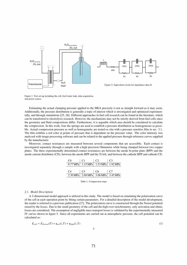
H2Ocrossover
/H2 out
H2O feed
H2Orecirculation
/O2 out
Potentiostat - +
Figure 1: Test set-up including the cell, feed water tank, data acquisition,and power source.
R1
CPE1
HFR
R2
CPE2
L
R3
CPE3
Figure 2: Equivalent circuit for impedance data fit
Estimating the actual clamping pressure applied to the MEA precisely is not as straight forward as it may seem.Additionally, the pressure distribution is generally a topic of interest which is investigated and optimized experimen-tally, and through simulations [25, 26]. Different approaches in fuel cell research can be found in the literature, whichcan be transferred to electrolysis research. However, the mechanisms may not be strictly derived from fuel cells sincethe geometry and fluid compositions differ. Furthermore, it is arguable which area should be considered to calculatethe compression. In this work, four die springs are used to establish a pressure distribution as homogeneous as possi-ble. Actual compression pressure as well as homogeneity are tested ex-situ with a pressure sensitive film in sec. 3.1.The film exhibits a red color at points of pressure that is dependent on the pressure value. The color intensity wasanalyzed with image processing software and can be related to the applied pressure through reference curves suppliedby the manufacturer.
Moreover, contact resistances are measured between several components that are accessible. Each contact isinvestigated separately through a sample with a high precision Ohmmeter while being clamped between two copperplates. The three experimentally determined contact resistances are between the anode bi-polar plate (BPP) and theanode current distributor (CD), between the anode BPP and the Ti felt, and between the cathode BPP and cathode CD.
C0 C1 C2 C30.77 MPa 1.15 MPa 1.53 MPa 1.92 MPa
C4 C5 C6 C72.30 MPa 2.68 MPa 3.06 MPa 3.45 MPa
Table 1: Compression steps
2.1. Model DescriptionA 2-dimensional model approach is utilized in this study. The model is based on simulating the polarization curve
of the cell at each operation point by fitting certain parameters. For a detailed description of the model development,the reader is referred to a previous publication [27]. The polarization curve is constructed through the Nernst potentialraised by the losses. Due to the small geometry of the cell and the high over-stoichiometry, only activation and ohmiclosses are considered. The assumption of negligible mass transport losses is validated by the experimentally measuredIV curves shown in figure 5. Since all experiments are carried out at atmospheric pressure, the cell potential can becalculated as:
Ecell = ENernst(T ) + ηact(i,T ) + ηohm(i,T ) (1)
3
71
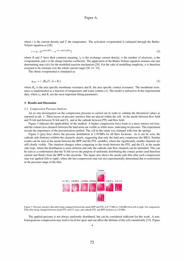
where i is the current density and T the temperature. The activation overpotential is estimated through the Butler-Volmer equation as [28]:
i = i0 · [eαnFη/(RT ) − e−(1−α)nFη/(RT )] (2)
where R and F have their common meaning, i0 is the exchange current density, n the number of electrons, η theoverpotential, and α is the charge transfer coefficient. The application of the Butler-Volmer equation assumes one ratedetermining step (rds) for the modelled reaction mechanism [29]. For the sake of modelling simplicity, α is thereforeassumed to be constant over the whole current range [30, 31, 32].
The ohmic overpotential is simulated as:
ηohm = i · [Rm(T, λ) + Rc] (3)
where Rm is the area specific membrane resistance and Rc the area specific contact resistance. The membrane resis-tance is implemented as a function of temperature and water content (λ). The model is utilized to fit the experimentaldata, where i0, and Rc are the most important fitting parameters.
3. Results and Discussion
3.1. Compression Pressure AnalysisAn ex-situ investigation on the compression pressure is carried out in order to validate the theoretical values as
reported in tab. 1. Three layers of pressure sensitive film are placed within the cell: At the anode between flow fieldand Ti felt and between Ti felt and CL, and at the cathode between PTL and flow field.
Figure 3 indicates the applicability of the method. A higher compression force leads to a more intense red tone,and the contact-less channels between the land areas are visible as white areas, indicating no pressure. The experimentreveals the importance of the pressurization method. The cell in this study was clamped with four die springs.
Figure 3 (grey box) shows the pressure distribution at 2.30 MPa for all three locations. As it can be seen, thecathode side (bottom) exhibits the channels clearly, suggesting that only the land area compresses the MEA. Similarresults can be seen at the anode between the BPP and the PTL (middle), where the significantly smaller channels arestill clearly visible. The situation changes when comparing to the result between the PTL and the CL at the anodeside (top), where the distribution is more uniform and only the cathode-side flow channels can be identified. This canbe seen as a confirmation that the Ti felt serves the purpose of uniformly distributing the contact points (and thereforecurrent and fluids) from the BPP to the electrode. The figure also shows the anode-side film after each compressionstep was applied (left to right), where the last compression step was not experimentally determined due to restrictionsin the pressure range of the film.
Figure 3: Pressure sensitive film after being clamped between the anode BPP and PTL at 0.77 MPa to 3.06 MPa from left to right. For comparison:Film after being clamped between anode PTL and CL (top), and cathode PTL and BPP (bottom) at 2.30 MPa
The applied pressure is not always uniformly distributed, but can be considered sufficient for this work. A non-homogeneous compression may lead to local hot spots and can affect the lifetime of the cell considerably [33]. Figure
4
Paper A.
72
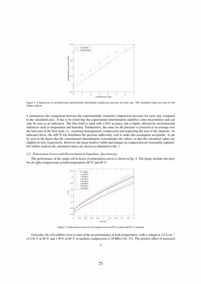
0 1 2 3 4 5 6 7
compression step
0.5
1
1.5
2
2.5
3
3.5
com
pres
sion
pre
ssur
e /M
Pa
CalculatedExperimental
Figure 4: Comparison of calculated and experimentally determined compression pressure for each step. The calculated values are used for thefurther analysis
4 summarizes the comparison between the experimentally extracted compression pressure for each step comparedto the calculated ones. It has to be noted that the experimental determination underlies some uncertainties and canonly be seen as an indication. The film itself is rated with ±10% accuracy, but is highly affected by environmentalinfluences such as temperature and humidity. Furthermore, the value for the pressure is extracted as an average overthe land area of the flow field, i.e., assuming homogeneous compression and neglecting the area of the channels. Asindicated above, the stiff Ti felt distributes the pressure sufficiently well to make this assumption acceptable. It canbe seen in the figure that the experimental determination overestimates the values, or that the calculated values areslightly too low, respectively. However, the linear trend is visible and changes in compression are reasonably captured.For further analysis the calculated values are chosen as tabulated in tab. 1.
3.2. Polarization Curves and Electrochemical Impedance Spectroscopy
The performance of the single cell in terms of polarization curves is shown in fig. 5. The figure includes the plotsfor all eight compressions at both temperatures 60 C and 80 C.
0 0.2 0.4 0.6 0.8 1 1.2 1.4 1.6 1.8 2
i /A*cm -2
1.4
1.5
1.6
1.7
1.8
1.9
2
2.1
V /V
0.77 MPa1.15 MPa1.53 MPa1.92 MPa2.30 MPa2.68 MPa3.06 MPa3.45 MPa
Figure 5: Polarization curves for all compressions at 60 C (solid) and 80 C (dashed)
Generally, the cell exhibits close to state of the art performance at both temperatures, with a voltage at 2.0 A cm−2
of 2.01 V at 60 C and 1.90 V at 80 C at medium compression (2.30 MPa) [34, 35]. The positive effect of increased
5
73
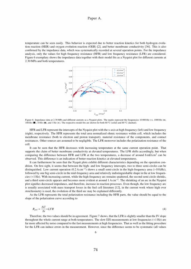
temperature can be seen easily. This behavior is expected due to better reaction kinetics for both hydrogen evolu-tion reaction (HER) and oxygen evolution reaction (OER) [2], and better membrane conductivity [36]. This is alsoconfirmed by the impedance data, which was systematically recorded at several operation points. For the impedanceanalysis, only the values for high frequency resistance (HFR) and low frequency resistance (LFR) are considered.Figure 6 exemplary shows the impedance data together with their model fits as a Nyquist plot for different currents at2.30 MPa and both temperatures.
0.15 0.2 0.25 0.3
Zreal
/ *cm2
-0.04
-0.02
0
0.02
0.04
0.06
0.08
Zim
g /
*cm
2
0.2 A*cm-2
0.5 A*cm-2
1.0 A*cm-2
Figure 6: Impedance data at 2.30 MPa and different currents as a Nyquist plots. The marks represent the frequencies 10 000 Hz (∗), 1000 Hz (•),100 Hz (), 10 Hz (), and 1 Hz (?). The respective model fits are shown for both 60 C (solid) and 80 C (dashed).
HFR and LFR represent the intercepts of the Nyquist plot with the x-axis at high frequency (left) and low frequency(right), respectively. The HFR represents the total area normalized ohmic resistance within cell, which includes themembrane resistance (both to electron and proton transport), material resistance of the components, and contactresistances. Other sources are assumed to be negligible. The LFR moreover includes the polarization resistance of thecell.
It can be seen that the HFR decreases with increasing temperature at the same current operation point. Thatsupports the claim of better membrane conductivity at elevated temperatures. The LFR shifts accordingly, but whencomparing the difference between HFR and LFR at the two temperatures, a decrease of around 6 mΩ cm2 can beobserved. This difference is an indication of better reaction kinetics at elevated temperatures.
It can furthermore be seen that the Nyquit plots exhibit different characteristics depending on the operation con-dition. On first sight, it seems that between the high- and low frequency intercepts, two to three semi-circles can bedistinguished. Low current operation (0.2 A cm−2) shows a small semi-circle in the high-frequency area (>10 kHz),followed by one big semi-circle in the mid-frequency area and relatively indistinguishable shape in the at low frequen-cies (<1 Hz). With increasing current, while the high frequency arc remains unaltered, the second semi circle shrinks,and a third semi-circle appears and becomes more evident at around 1 A cm−2. The shrinking of an arc in the Nyquistplot signifies decreased impedance, and therefore, increase in reaction processes. Even though, the low frequency arcis usually associated with mass transport losses in the fuel cell literature [12], in the current work where high overstoichiometry is used, the evolution of the third arc may be explained differently.
As the LFR represents the total polarization resistance including the HFR parts, the value should be equal to theslope of the polarization curve according to
Rpol =∆U∆i
=LFR (4)
Therefore, the two values should be in agreement. Figure 7 shows, that the LFR is slightly smaller than the IV slopethroughout the whole current range at both temperatures. The slow EIS measurements at low frequencies (<1 Hz) arefar more affected by noise compared to the fast measurements at high frequencies. That as well as the fitting procedurefor the LFR can induce errors in the measurement. However, since the difference seems to be systematic (all values
6
Paper A.
74
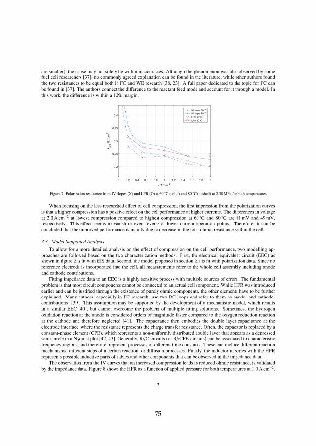
are smaller), the cause may not solely lie within inaccuracies. Although the phenomenon was also observed by somefuel cell researchers [37], no commonly agreed explanation can be found in the literature, while other authors foundthe two resistances to be equal both in FC and WE research [38, 23]. A full paper dedicated to the topic for FC canbe found in [37]. The authors connect the difference to the reactant feed mode and account for it through a model. Inthis work, the difference is within a 12% margin.
0 0.2 0.4 0.6 0.8 1 1.2 1.4 1.6 1.8 2
i /A*cm -2
0.2
0.25
0.3
0.35
0.4
Rpo
l /*c
m2
IV slope 60°CIV slope 80°CLFR 60°CLFR 80°C
Figure 7: Polarization resistance from IV slopes (X) and LFR (O) at 60 C (solid) and 80 C (dashed) at 2.30 MPa for both temperatures
When focusing on the less researched effect of cell compression, the first impression from the polarization curvesis that a higher compression has a positive effect on the cell performance at higher currents. The differences in voltageat 2.0 A cm−2 at lowest compression compared to highest compression at 60 C and 80 C are 81 mV and 49 mV,respectively. This effect seems to vanish or even reverse at lower current operation points. Therefore, it can beconcluded that the improved performance is mainly due to decrease in the total ohmic resistance within the cell.
3.3. Model Supported Analysis
To allow for a more detailed analysis on the effect of compression on the cell performance, two modelling ap-proaches are followed based on the two characterization methods: First, the electrical equivalent circuit (EEC) asshown in figure 2 is fit with EIS data. Second, the model proposed in section 2.1 is fit with polarization data. Since noreference electrode is incorporated into the cell, all measurements refer to the whole cell assembly including anodeand cathode contributions.
Fitting impedance data to an EEC is a highly sensitive process with multiple sources of errors. The fundamentalproblem is that most circuit components cannot be connected to an actual cell component. While HFR was introducedearlier and can be justified through the existence of purely ohmic components, the other elements have to be furtherexplained. Many authors, especially in FC research, use two RC-loops and refer to them as anode- and cathode-contributions [39]. This assumption may be supported by the development of a mechanistic model, which resultsin a similar EEC [40], but cannot overcome the problem of multiple fitting solutions. Sometimes, the hydrogenoxidation reaction at the anode is considered orders of magnitude faster compared to the oxygen reduction reactionat the cathode and therefore neglected [41]. The capacitance then embodies the double layer capacitance at theelectrode interface, where the resistance represents the charge transfer resistance. Often, the capacitor is replaced by aconstant-phase element (CPE), which represents a non-uniformly distributed double layer that appears as a depressedsemi-circle in a Nyquist plot [42, 43]. Generally, R//C-circuits (or R//CPE-circuits) can be associated to characteristicfrequency regions, and therefore, represent processes of different time constants. These can include different reactionmechanisms, different steps of a certain reaction, or diffusion processes. Finally, the inductor in series with the HFRrepresents possible inductive parts of cables and other components that can be observed in the impedance data.
The observation from the IV curves that an increased compression leads to reduced ohmic resistance, is validatedby the impedance data. Figure 8 shows the HFR as a function of applied pressure for both temperatures at 1.0 A cm−2.
7
75
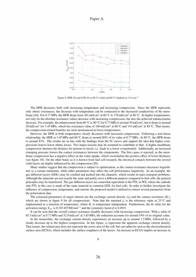
0.5 1 1.5 2 2.5 3 3.5
c /MPa
0.14
0.16
0.18
0.2
0.22
0.24
0.26
0.28
0.3
0.32
Rre
al /
*cm
2
HFR 60°CHFR 80°CLFR 60°CLFR 80°C
Figure 8: HFR (X) and LFR (O) at 60 C (solid) and 80 C (dashed) at 1.0 A cm−2
The HFR decreases both with increasing temperature and increasing compression. Since the HFR representsonly ohmic resistances, the decrease with temperature can be connected to the increased conductivity of the mem-brane [44]. For 0.77 MPa, the HFR drops from 201 mΩ cm2 at 60 C to 170 mΩ cm2 at 80 C. At higher temperatures,not only do the absolute resistance values decrease with increasing compression, but also the achieved enhancementsdecrease. For example, the enhancement from 60 C to 80 C for 0.77 MPa is around 30 mΩ cm2, but it drops to around20 mΩ cm2 for 3.45 MPa, which has resistance value of 160 mΩ cm2 at 60 C and 141 mΩ cm2 at 80 C. That means,the compression-related benefits are more pronounced at lower temperatures.
However, the HFR at both temperatures clearly decreases with increased compression. Following a non-linearrelationship, the HFR at 3.45 MPa and 60 C drops to around 80% of its value at 0.77 MPa. At 80 C, the HFR dropsto around 83%. The results are in line with the findings from the IV curves and support the idea that higher com-pressions lead to lower ohmic losses. Two major reasons may be assumed to contribute to that: A higher membranecompression shortens the distance for protons to travel, i.e. leads to a lower overpotential. Additionally, an increasedclamping pressure lowers the contact resistances between the components. The first cause is rejected, as the mem-brane compression has a negative effect on the water uptake, which overwhelms the positive effect of lower thickness(see figure 10). On the other hand, as it is known from fuel cell research, the electrical contacts between the severalsolid layers are highly influenced by the compression [20].
Many studies suggest that the compression is subject to optimization, as the contact resistance decreases logarith-mic to a certain minimum, while other parameters may affect the cell performance negatively. As an example, thegas diffusion layers (GDL) may be crushed and pushed into the channels, which results in mass transport problems.Although the materials are not exactly the same and partly serve a different purpose compared to fuel cells, the generalprinciples may be transferred. The gas diffusion layers are somewhat equivalent to the PTL in WE, where the cathodeside PTL in this case is made of the same material as common GDL for fuel cells. In order to further investigate theinfluence of compression, temperature, and current, the proposed model is utilized to extract several parameters fromthe polarization data.
The extracted parameters of major interest are the exchange current density (i0) and the contact resistance (Rc),which are shown in figure 9 for all compressions. Note that the reported i0 is the reference value at 25 C andimplemented as a function of temperature, where Rc is temperature independent. Furthermore, the fit value for theactivation energy Eact is 0.103 455 MJ mol−1 and the symmetry factor β is 0.4931
It can be seen that the overall contact resistance steadily decreases with increasing compression. With a value of65.3 mΩ cm2 at 0.77 MPa and 52.9 mΩ cm2 at 3.45 MPa, the reduction accounts for around 19% of its original value.
In the meanwhile, the exchange current density experiences an increase up to around 1.5 MPa, followed by asteady decrease up to the highest compression. In this figure, i0 represents the apparent exchange current density.That means, the related area does not represent the active area of the cell, but can rather be seen as the electrochemicalsurface area (ECSA), which includes the surface roughness of the layers. An increase in ECSA implies an increase in
8
Paper A.
76
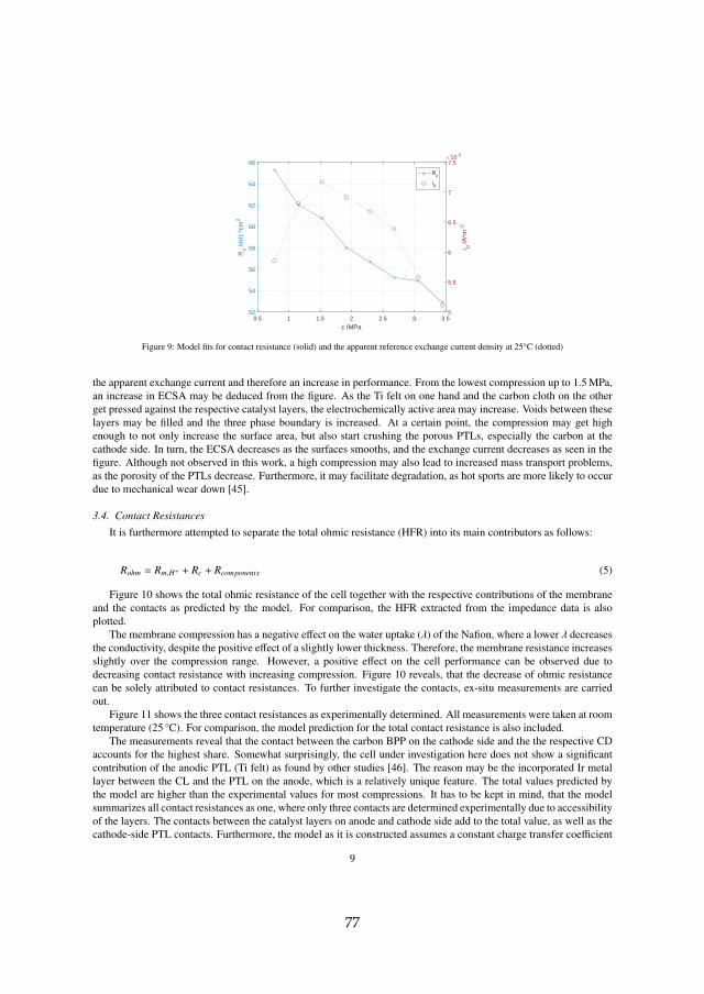
0.5 1 1.5 2 2.5 3 3.5
c /MPa
52
54
56
58
60
62
64
66
Rc /m
*cm
2
5
5.5
6
6.5
7
7.5
i 0 /A
*m-2
10-5
Rc
i0
Figure 9: Model fits for contact resistance (solid) and the apparent reference exchange current density at 25°C (dotted)
the apparent exchange current and therefore an increase in performance. From the lowest compression up to 1.5 MPa,an increase in ECSA may be deduced from the figure. As the Ti felt on one hand and the carbon cloth on the otherget pressed against the respective catalyst layers, the electrochemically active area may increase. Voids between theselayers may be filled and the three phase boundary is increased. At a certain point, the compression may get highenough to not only increase the surface area, but also start crushing the porous PTLs, especially the carbon at thecathode side. In turn, the ECSA decreases as the surfaces smooths, and the exchange current decreases as seen in thefigure. Although not observed in this work, a high compression may also lead to increased mass transport problems,as the porosity of the PTLs decrease. Furthermore, it may facilitate degradation, as hot sports are more likely to occurdue to mechanical wear down [45].
3.4. Contact Resistances
It is furthermore attempted to separate the total ohmic resistance (HFR) into its main contributors as follows:
Rohm = Rm,H+ + Rc + Rcomponents (5)
Figure 10 shows the total ohmic resistance of the cell together with the respective contributions of the membraneand the contacts as predicted by the model. For comparison, the HFR extracted from the impedance data is alsoplotted.
The membrane compression has a negative effect on the water uptake (λ) of the Nafion, where a lower λ decreasesthe conductivity, despite the positive effect of a slightly lower thickness. Therefore, the membrane resistance increasesslightly over the compression range. However, a positive effect on the cell performance can be observed due todecreasing contact resistance with increasing compression. Figure 10 reveals, that the decrease of ohmic resistancecan be solely attributed to contact resistances. To further investigate the contacts, ex-situ measurements are carriedout.
Figure 11 shows the three contact resistances as experimentally determined. All measurements were taken at roomtemperature (25 C). For comparison, the model prediction for the total contact resistance is also included.
The measurements reveal that the contact between the carbon BPP on the cathode side and the the respective CDaccounts for the highest share. Somewhat surprisingly, the cell under investigation here does not show a significantcontribution of the anodic PTL (Ti felt) as found by other studies [46]. The reason may be the incorporated Ir metallayer between the CL and the PTL on the anode, which is a relatively unique feature. The total values predicted bythe model are higher than the experimental values for most compressions. It has to be kept in mind, that the modelsummarizes all contact resistances as one, where only three contacts are determined experimentally due to accessibilityof the layers. The contacts between the catalyst layers on anode and cathode side add to the total value, as well as thecathode-side PTL contacts. Furthermore, the model as it is constructed assumes a constant charge transfer coefficient
9
77
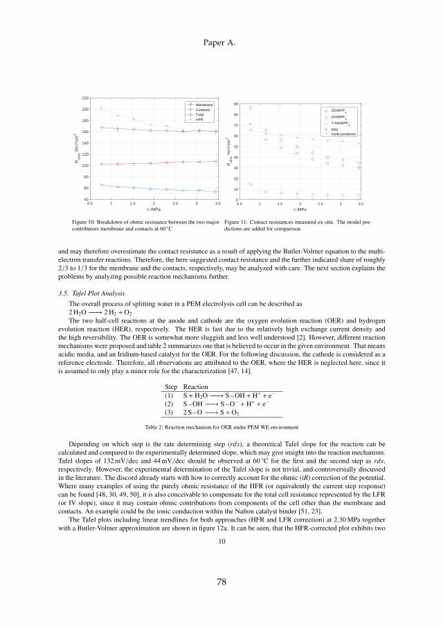
0.5 1 1.5 2 2.5 3 3.5
c /MPa
40
60
80
100
120
140
160
180
200
220
Roh
m /m
*cm
2
MembraneContactsTotalHFR
Figure 10: Breakdown of ohmic resistance between the two majorcontributors membrane and contacts at 60 C
0.5 1 1.5 2 2.5 3 3.5
c /MPa
0
10
20
30
40
50
60
70
80
90
Roh
m /m
*cm
2
CD//BPPc
CD//BPPa
Ti felt//BPPa
totalmodel prediction
Figure 11: Contact resistances measured ex-situ. The model pre-dictions are added for comparison
and may therefore overestimate the contact resistance as a result of applying the Butler-Volmer equation to the multi-electron transfer reactions. Therefore, the here suggested contact resistance and the further indicated share of roughly2/3 to 1/3 for the membrane and the contacts, respectively, may be analyzed with care. The next section explains theproblems by analyzing possible reaction mechanisms further.
3.5. Tafel Plot Analysis
The overall process of splitting water in a PEM electrolysis cell can be described as2 H2O −−−→ 2 H2 + O2The two half-cell reactions at the anode and cathode are the oxygen evolution reaction (OER) and hydrogen
evolution reaction (HER), respectively. The HER is fast due to the relatively high exchange current density andthe high reversibility. The OER is somewhat more sluggish and less well understood [2]. However, different reactionmechanisms were proposed and table 2 summarizes one that is believed to occur in the given environment. That meansacidic media, and an Iridium-based catalyst for the OER. For the following discussion, the cathode is considered as areference electrode. Therefore, all observations are attributed to the OER, where the HER is neglected here, since itis assumed to only play a minor role for the characterization [47, 14].
Step Reaction(1) S + H2O −−−→ S – OH + H+ + e–
(2) S – OH −−−→ S – O– + H+ + e–
(3) 2 S – O −−−→ S + O2
Table 2: Reaction mechanism for OER under PEM WE environment
Depending on which step is the rate determining step (rds), a theoretical Tafel slope for the reaction can becalculated and compared to the experimentally determined slope, which may give insight into the reaction mechanism.Tafel slopes of 132 mV/dec and 44 mV/dec should be observed at 60 C for the first and the second step as rds,respectively. However, the experimental determination of the Tafel slope is not trivial, and controversially discussedin the literature. The discord already starts with how to correctly account for the ohmic (iR) correction of the potential.Where many examples of using the purely ohmic resistance of the HFR (or equivalently the current step response)can be found [48, 30, 49, 50], it is also conceivable to compensate for the total cell resistance represented by the LFR(or IV slope), since it may contain ohmic contributions from components of the cell other than the membrane andcontacts. An example could be the ionic conduction within the Nafion catalyst binder [51, 23].
The Tafel plots including linear trendlines for both approaches (HFR and LFR correction) at 2.30 MPa togetherwith a Butler-Volmer approximation are shown in figure 12a. It can be seen, that the HFR-corrected plot exhibits two
10
Paper A.
78
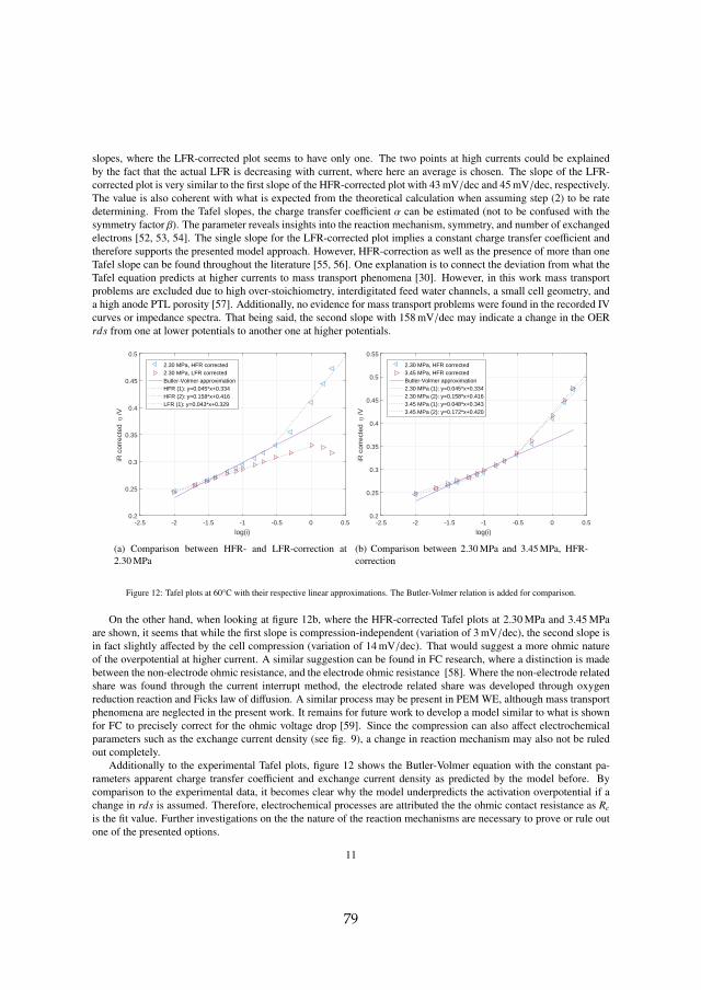
slopes, where the LFR-corrected plot seems to have only one. The two points at high currents could be explainedby the fact that the actual LFR is decreasing with current, where here an average is chosen. The slope of the LFR-corrected plot is very similar to the first slope of the HFR-corrected plot with 43 mV/dec and 45 mV/dec, respectively.The value is also coherent with what is expected from the theoretical calculation when assuming step (2) to be ratedetermining. From the Tafel slopes, the charge transfer coefficient α can be estimated (not to be confused with thesymmetry factor β). The parameter reveals insights into the reaction mechanism, symmetry, and number of exchangedelectrons [52, 53, 54]. The single slope for the LFR-corrected plot implies a constant charge transfer coefficient andtherefore supports the presented model approach. However, HFR-correction as well as the presence of more than oneTafel slope can be found throughout the literature [55, 56]. One explanation is to connect the deviation from what theTafel equation predicts at higher currents to mass transport phenomena [30]. However, in this work mass transportproblems are excluded due to high over-stoichiometry, interdigitated feed water channels, a small cell geometry, anda high anode PTL porosity [57]. Additionally, no evidence for mass transport problems were found in the recorded IVcurves or impedance spectra. That being said, the second slope with 158 mV/dec may indicate a change in the OERrds from one at lower potentials to another one at higher potentials.
-2.5 -2 -1.5 -1 -0.5 0 0.5
log(i)
0.2
0.25
0.3
0.35
0.4
0.45
0.5
iR c
orre
cted
/V
2.30 MPa, HFR corrected2.30 MPa, LFR correctedButler-Volmer approximationHFR (1): y=0.045*x+0.334HFR (2): y=0.158*x+0.416LFR (1): y=0.043*x+0.329
(a) Comparison between HFR- and LFR-correction at2.30 MPa
-2.5 -2 -1.5 -1 -0.5 0 0.5
log(i)
0.2
0.25
0.3
0.35
0.4
0.45
0.5
0.55iR
cor
rect
ed
/V2.30 MPa, HFR corrected3.45 MPa, HFR correctedButler-Volmer approximation2.30 MPa (1): y=0.045*x+0.3342.30 MPa (2): y=0.158*x+0.4163.45 MPa (1): y=0.048*x+0.3433.45 MPa (2): y=0.172*x+0.420
(b) Comparison between 2.30 MPa and 3.45 MPa, HFR-correction
Figure 12: Tafel plots at 60°C with their respective linear approximations. The Butler-Volmer relation is added for comparison.
On the other hand, when looking at figure 12b, where the HFR-corrected Tafel plots at 2.30 MPa and 3.45 MPaare shown, it seems that while the first slope is compression-independent (variation of 3 mV/dec), the second slope isin fact slightly affected by the cell compression (variation of 14 mV/dec). That would suggest a more ohmic natureof the overpotential at higher current. A similar suggestion can be found in FC research, where a distinction is madebetween the non-electrode ohmic resistance, and the electrode ohmic resistance [58]. Where the non-electrode relatedshare was found through the current interrupt method, the electrode related share was developed through oxygenreduction reaction and Ficks law of diffusion. A similar process may be present in PEM WE, although mass transportphenomena are neglected in the present work. It remains for future work to develop a model similar to what is shownfor FC to precisely correct for the ohmic voltage drop [59]. Since the compression can also affect electrochemicalparameters such as the exchange current density (see fig. 9), a change in reaction mechanism may also not be ruledout completely.
Additionally to the experimental Tafel plots, figure 12 shows the Butler-Volmer equation with the constant pa-rameters apparent charge transfer coefficient and exchange current density as predicted by the model before. Bycomparison to the experimental data, it becomes clear why the model underpredicts the activation overpotential if achange in rds is assumed. Therefore, electrochemical processes are attributed the the ohmic contact resistance as Rc
is the fit value. Further investigations on the the nature of the reaction mechanisms are necessary to prove or rule outone of the presented options.
11
79
4. Conclusion
The effect of clamping pressure at various currents and temperatures on a state of the art PEM WE cell wereinvestigated. Where a clear influence can already be seen in the polarization curves, electrochemical impedancespectroscopy and Tafel plots were utilized to further narrow down the analysis. Additionally, a mathematical modelwas utilized to extract exchange current density and contact resistance. The exchange current density seems to have anoptimal value of compression at around 1.5 MPa, where the contact resistance decreases throughout the whole rangeof investigated compressions. That was further supported by ex-situ contact resistance measurements. Compared tothe contacts, the membrane is the dominant contributor to the ohmic losses within the cell. A Tafel plot analysisrevealed a certain disagreement in the literature. The proposed explanations include a change in rate determining stepfor the oxygen evolution reaction.
Besides the positive effect on cell performance, it should be kept in mind, that both increased temperature andcompression may have a negative effect on the lifetime of the cell due to formation of hot spots. That is investigatedin on-going work.
Acknowledgement
The authors would like to acknowledge the support by Innovation Fund Denmark through the e-STORE project,Grant 4106-00025B.
References
[1] International Energy Agency (IEA), Technology Roadmap: Hydrogen and Fuel Cells, Tech. rep., IEA (2015).doi:10.1007/SpringerReference 7300.
[2] A. Godula-Jopek, Hydrogen Production by Electrolysis, Wiley-VCH, 2015.[3] F. Gutierrez-Martın, I. Guerrero-Hernandez, Balancing the grid loads by large scale integration of hydrogen technologies: The case of the
Spanish power system, International Journal of Hydrogen Energy 37 (2) (2012) 1151–1161. doi:10.1016/j.ijhydene.2011.09.116.[4] D. Bessarabov, H. Wang, H. Li, N. Zhao, PEM Electrolysis for Hydrogen Production - Principles and Applications, CRC Press, 2016.[5] M. Carmo, D. L. Fritz, J. Mergel, D. Stolten, A comprehensive review on PEM water electrolysis, International Journal of Hydrogen Energy
38 (12) (2013) 4901–4934.[6] F. Barbir, PEM electrolysis for production of hydrogen from renewable energy sources, Solar Energy 78 (5) (2005) 661–669.
doi:10.1016/j.solener.2004.09.003.[7] S. A. Grigoriev, V. I. Porembskiy, S. V. Korobtsev, V. N. Fateev, F. Aupre, P. Millet, High-pressure PEM water electrolysis and corresponding
safety issues, International Journal of Hydrogen Energy 6 (2010) 3–10. doi:10.1016/j.ijhydene.2010.03.058.[8] B. Bensmann, R. Hanke-Rauschenbach, I. K. Pena Arias, K. Sundmacher, Energetic evaluation of high pressure PEM electrolyzer systems
for intermediate storage of renewable energies, Electrochimica Acta 110 (2013) 570–580. doi:10.1016/j.electacta.2013.05.102.[9] F. N. Buchi, S. A. Freunberger, M. Reum, G. Paganelli, A. Tsukada, P. Dietrich, A. Delfino, On the efficiency of an advanced automotive fuel
cell system, Fuel Cells 7 (2) (2007) 159–164. doi:10.1002/fuce.200500257.[10] A. S. Arico, S. Siracusano, N. Briguglio, V. Baglio, A. Di Blasi, V. Antonucci, Polymer electrolyte membrane water electrolysis: Status of
technologies and potential applications in combination with renewable power sources, Journal of Applied Electrochemistry 43 (2) (2013)107–118. doi:10.1007/s10800-012-0490-5.
[11] C. A. Martinson, G. van Schoor, K. R. Uren, D. Bessarabov, Characterisation of a PEM electrolyser using the current interrupt method,International Journal of Hydrogen Energy 39 (36) (2014) 20865–20878. doi:10.1016/j.ijhydene.2014.09.153.URL http://dx.doi.org/10.1016/j.ijhydene.2014.09.153
[12] X. Yuan, H. Wang, J. Colinsun, J. Zhang, AC impedance technique in PEM fuel cell diagnosisA review, International Journal of HydrogenEnergy 32 (17) (2007) 4365–4380. doi:10.1016/j.ijhydene.2007.05.036.
[13] J. Wu, X. Z. Yuan, H. Wang, M. Blanco, J. J. Martin, J. Zhang, Diagnostic tools in PEM fuel cell research: Part I Electrochemical techniques,International Journal of Hydrogen Energy 33 (6) (2008) 1735–1746. doi:10.1016/j.ijhydene.2008.01.013.
[14] C. Rozain, P. Millet, Electrochemical characterization of Polymer Electrolyte Membrane Water Electrolysis Cells, Electrochimica Acta 131(2014) 160–167. doi:10.1016/j.electacta.2014.01.099.URL http://dx.doi.org/10.1016/j.electacta.2014.01.099
[15] J. Van Der Merwe, K. Uren, G. Van Schoor, D. Bessarabov, Characterisation tools development for PEM electrolysers, International Journalof Hydrogen Energy 39 (26) (2014) 14212–14221. doi:10.1016/j.ijhydene.2014.02.096.URL http://dx.doi.org/10.1016/j.ijhydene.2014.02.096
[16] H. Su, B. J. Bladergroen, S. Pasupathi, V. Linkov, S. Ji, Performance investigation of membrane electrode assemblies for hydrogen productionby solid polymer electrolyte water electrolysis, International Journal of Electrochemical Science 7 (5) (2012) 4223–4234.
[17] B. S. Lee, H. Y. Park, I. Choi, M. K. Cho, H. J. Kim, S. J. Yoo, D. Henkensmeier, J. Y. Kim, S. W. Nam, S. Park, K. Y. Lee, J. H. Jang,Polarization characteristics of a low catalyst loading PEM water electrolyzer operating at elevated temperature, Journal of Power Sources 309(2016) 127–134. doi:10.1016/j.jpowsour.2015.12.139.URL http://dx.doi.org/10.1016/j.jpowsour.2015.12.139
12
Paper A.
80
[18] I. Dedigama, P. Angeli, K. Ayers, J. B. Robinson, P. R. Shearing, D. Tsaoulidis, D. J. L. Brett, In situ diagnostic techniques for characterisationof polymer electrolyte membrane water electrolysers - Flow visualisation and electrochemical impedance spectroscopy, International Journalof Hydrogen Energy 39 (9) (2014) 4468–4482. doi:10.1016/j.ijhydene.2014.01.026.URL http://dx.doi.org/10.1016/j.ijhydene.2014.01.026
[19] S. Sun, Y. Xiao, D. Liang, Z. Shao, H. Yu, M. Hou, B. Yi, Behaviors of a proton exchange membrane electrolyzer under water starvation,RSC Adv. 5 (19) (2015) 14506–14513. doi:10.1039/C4RA14104K.URL http://xlink.rsc.org/?DOI=C4RA14104K
[20] J. Millichamp, T. J. Mason, T. P. Neville, N. Rajalakshmi, R. Jervis, P. R. Shearing, D. J. L. Brett, Mechanisms and effects of mechan-ical compression and dimensional change in polymer electrolyte fuel cells - A review, Journal of Power Sources 284 (2015) 305–320.doi:10.1016/j.jpowsour.2015.02.111.URL http://dx.doi.org/10.1016/j.jpowsour.2015.02.111
[21] S. Asghari, A. Mokmeli, M. Samavati, Study of PEM fuel cell performance by electrochemical impedance spectroscopy, International Journalof Hydrogen Energy 35 (17) (2010) 9283–9290. doi:10.1016/j.ijhydene.2010.03.069.URL http://dx.doi.org/10.1016/j.ijhydene.2010.03.069
[22] A. Diedrichs, M. Rastedt, F. J. Pinar, P. Wagner, Effect of compression on the performance of a HT-PEM fuel cell, Journal of AppliedElectrochemistry 43 (11) (2013) 1079–1099. doi:10.1007/s10800-013-0597-3.
[23] K. Elsøe, L. Grahl-Madsen, G. G. Scherer, J. Hjelm, M. B. Mogensen, Electrochemical Characterization of a PEMEC Using ImpedanceSpectroscopy, Journal of The Electrochemical Society 164 (13) (2017) F1419–F1426. doi:10.1149/2.0651713jes.URL http://jes.ecsdl.org/lookup/doi/10.1149/2.0651713jes
[24] S. Siracusano, V. Baglio, S. A. Grigoriev, L. Merlo, V. N. Fateev, A. S. Arico, A PEM water electrolyser based on metallic Iridium electro-catalyst, Pt/C and Aquivion membrane (2017).
[25] A. Bates, S. Mukherjee, S. Hwang, S. C. Lee, O. Kwon, G. H. Choi, S. Park, Simulation and experimental analysis of theclamping pressure distribution in a PEM fuel cell stack, International Journal of Hydrogen Energy 38 (15) (2013) 6481–6493.doi:10.1016/j.ijhydene.2013.03.049.URL http://dx.doi.org/10.1016/j.ijhydene.2013.03.049
[26] E. Alizadeh, M. Ghadimi, M. M. Barzegari, M. Momenifar, S. H. Saadat, Development of contact pressure distribution of PEM fuel cell’sMEA using novel clamping mechanism, Energy 131 (2017) 92–97. doi:10.1016/j.energy.2017.05.036.URL http://dx.doi.org/10.1016/j.energy.2017.05.036
[27] A. C. Olesen, S. K. Kær, The Effect of PFSA Membrane Compression on the Predicted Performance of a High Pressure PEM ElectrolysisCell, ECS Transactions 68 (3) (2015) 99–116. doi:10.1149/06803.0099ecst.
[28] R. O’Hayre, S.-W. Cha, W. Colella, F. B. Prinz, Fuel Cell Fundamentals, John Wiley and Sons, 2006.[29] R. F. Mann, J. C. Amphlett, B. A. Peppley, C. P. Thurgood, Application of Butler Volmer equations in the modelling of activation polarization
for PEM fuel cells, Journal of Power Sources 161 (2006) 775–781. doi:10.1016/j.jpowsour.2006.05.026.[30] M. Suermann, T. J. Schmidt, F. N. Buchi, Cell Performance Determining Parameters in High Pressure Water Electrolysis, Electrochimica
Acta 211 (2016) 989–997. doi:10.1016/j.electacta.2016.06.120.[31] F. Marangio, M. Santarelli, M. Calı, Theoretical model and experimental analysis of a high pressure PEM water electrolyser for hydrogen
production, International Journal of Hydrogen Energy 34 (3) (2009) 1143–1158. doi:10.1016/j.ijhydene.2008.11.083.[32] Z. Abdin, C. J. Webb, E. M. Gray, Modelling and simulation of a proton exchange membrane ( PEM ) electrolyser cell, International Journal
of Hydrogen Energy 40 (39) (2015) 13243–13257. doi:10.1016/j.ijhydene.2015.07.129.URL http://dx.doi.org/10.1016/j.ijhydene.2015.07.129
[33] T. Hottinen, O. Himanen, S. Karvonen, I. Nitta, T. Hottinen, O. Himanen, M. Mikkola, S. Karvonen, I. Nitta, Inhomogeneous compressionof PEMFC gas diffusion layer. Part II. Modeling the effect, Journal of Power Sources 171 (1) (2007) 113–121.
[34] C. Rozain, E. Mayousse, N. Guillet, P. Millet, Influence of iridium oxide loadings on the performance of PEM water electrolysis cells : PartI Pure IrO 2 -based anodes, ”Applied Catalysis B, Environmental” 182 (2016) 153–160. doi:10.1016/j.apcatb.2015.09.013.URL http://dx.doi.org/10.1016/j.apcatb.2015.09.013
[35] S. Siracusano, V. Baglio, E. Moukheiber, L. Merlo, A. S. Arico, Performance of a PEM water electrolyser combining an IrRu-oxide an-ode electrocatalyst and a shortside chain Aquivion membrane, International Journal of Hydrogen Energy 40 (42) (2015) 14430–14435.doi:10.1016/j.ijhydene.2015.04.159.
[36] T. a. Zawodzinski, Water Uptake by and Transport Through Nafion® 117 Membranes, Journal of The Electrochemical Society 140 (4) (1993)1041. doi:10.1149/1.2056194.
[37] M. Chandesris, C. Robin, M. Gerard, Y. Bultel, Investigation of the difference between the low frequency limit of the impedance spectrumand the slope of the polarization curve, Electrochimica Acta 180 (2015) 581–590. doi:10.1016/j.electacta.2015.08.089.URL http://dx.doi.org/10.1016/j.electacta.2015.08.089
[38] I. Pivac, F. Barbir, Inductive phenomena at low frequencies in impedance spectra of proton exchange membrane fuel cells - A review, Journalof Power Sources 326 (2016) 112–119. doi:10.1016/j.jpowsour.2016.06.119.URL http://dx.doi.org/10.1016/j.jpowsour.2016.06.119
[39] A. M. Dhirde, N. V. Dale, H. Salehfar, M. D. Mann, T. H. Han, Equivalent electric circuit modeling and performance analysis of a PEM fuelcell stack using impedance spectroscopy, IEEE Transactions on Energy Conversion 25 (3) (2010) 778–786. doi:10.1109/TEC.2010.2049267.
[40] S. M. R. Niya, R. K. Phillips, M. Hoorfar, Process modeling of the impedance characteristics of proton exchange membrane fuel cells,Electrochimica Acta 191 (2016) 594–605. doi:10.1016/j.electacta.2016.01.128.
[41] M. A. Rubio, A. Urquia, R. Kuhn, S. Dormido, Electrochemical parameter estimation in operating proton exchange membrane fuel cells,Journal of Power Sources 183 (1) (2008) 118–125. doi:10.1016/j.jpowsour.2008.05.011.
[42] M. E. Orazem, N. Pebere, B. Tribollet, Enhanced Graphical Representation of Electrochemical Impedance Data, Journal of The Electrochem-ical Society 153 (4) (2006) 129. doi:10.1149/1.2168377.
[43] P. Cordoba-Torres, T. J. Mesquita, O. Devos, B. Tribollet, V. Roche, R. P. Nogueira, On the intrinsic coupling between
13
81
constant-phase element parameters ?? and Q in electrochemical impedance spectroscopy, Electrochimica Acta 72 (2012) 172–178.doi:10.1016/j.electacta.2012.04.020.URL http://dx.doi.org/10.1016/j.electacta.2012.04.020
[44] H. Ito, T. Maeda, A. Nakano, H. Takenaka, Properties of Nafion membranes under PEM water electrolysis conditions, International Journalof Hydrogen Energy 36 (17) (2011) 10527–10540. doi:10.1016/j.ijhydene.2011.05.127.URL http://dx.doi.org/10.1016/j.ijhydene.2011.05.127
[45] Q. Feng, X. Yuan, G. Liu, B. Wei, Z. Zhang, H. Li, H. Wang, A review of proton exchange membrane water electrolysis on degradationmechanisms and mitigation strategies, Journal of Power Sources 366 (2017) 33–55. doi:10.1016/j.jpowsour.2017.09.006.URL http://dx.doi.org/10.1016/j.jpowsour.2017.09.006
[46] P. Lettenmeier, S. Kolb, F. Burggraf, A. S. Gago, K. A. Friedrich, Towards developing a backing layer for proton exchange membraneelectrolyzers, Journal of Power Sources 311 (2016) 153–158. doi:10.1016/j.jpowsour.2016.01.100.URL http://dx.doi.org/10.1016/j.jpowsour.2016.01.100
[47] E. Brightman, J. Dodwell, N. Van Dijk, G. Hinds, In situ characterisation of PEM water electrolysers using a novel reference electrode,Electrochemistry Communications 52 (2015) 1–4. doi:10.1016/j.elecom.2015.01.005.URL http://dx.doi.org/10.1016/j.elecom.2015.01.005
[48] K. S. Kadakia, P. Jampani, O. I. Velikokhatnyi, M. K. Datta, S. J. Chung, J. a. Poston, A. Manivannan, P. N. Kumta, Nanostructured(Ir,Sn)O2:F - Oxygen Evolution Reaction Anode Electro-Catalyst Powders for PEM Based Water Electrolysis, Journal of the ElectrochemicalSociety 161 (9) (2014) F868–F875. doi:10.1149/2.0381409jes.URL http://jes.ecsdl.org/cgi/doi/10.1149/2.0381409jes
[49] Gamry Instruments, Understanding iR Compensation (2017).[50] A. J. Bard, G. Inzelt, F. Scholz, Electrochemical dictionary, Springer-Verlag, 2008.[51] M. Bernt, H. A. H. Gasteiger, Influence of Ionomer Content in IrO 2 /TiO 2 Electrodes on PEM Water Electrolyzer Performance, Journal of
The Electrochemical Society 163 (11) (2016) F3179–F3189. doi:10.1149/2.0231611jes.URL http://jes.ecsdl.org/lookup/doi/10.1149/2.0231611jes
[52] J. Bockris, Z. Nagy, Symmetry Factor and Transfer Coefficient, Journal of Chemical Education.[53] M. Noel, K. Vasu, Charge Tranfer Kinetics and Diffusion, in: Cyclic Voltammetry and the Frontiers of Electrochemistry, Oxford & IBH
Publishing Co. Pvt. Ltd., New Delhi, 1990, pp. 157–194.URL http://noel-cyclic-voltametric-one.tripod.com/cvm/Chapter-4.PDF
[54] R. Guidelli, R. G. Compton, J. M. Feliu, E. Gileadi, J. Lipkowski, W. Schmickler, S. Trasatti, Defining the transfer coefficient in electrochem-istry: An assessment (IUPAC Technical Report), Pure and Applied Chemistry 86 (2) (2014) 245–258. doi:10.1515/pac-2014-5026.URL http://www.degruyter.com/view/j/pac.2014.86.issue-2/pac-2014-5026/pac-2014-5026.xml
[55] J. M. Hu, J. Q. Zhang, C. N. Cao, Oxygen evolution reaction on IrO2-based DSA?? type electrodes: Kinetics analysis of Tafel lines and EIS,International Journal of Hydrogen Energy 29 (8) (2004) 791–797. doi:10.1016/j.ijhydene.2003.09.007.
[56] E. Slavcheva, I. Radev, S. Bliznakov, G. Topalov, P. Andreev, E. Budevski, Sputtered iridium oxide films as electrocatalysts for water splittingvia PEM electrolysis, Electrochimica Acta 52 (12) (2007) 3889–3894. doi:10.1016/j.electacta.2006.11.005.
[57] U. Babic, M. Suermann, F. N. Buchi, L. Gubler, T. J. Schmidt, Critical ReviewIdentifying Critical Gaps for Polymer Electrolyte WaterElectrolysis Development, Journal of The Electrochemical Society 164 (4) (2017) F387–F399. doi:10.1149/2.1441704jes.URL http://jes.ecsdl.org/lookup/doi/10.1149/2.1441704jes
[58] M. V. Williams, H. R. Kunz, J. M. Fenton, Analysis of Polarization Curves to Evaluate Polarization Sources in Hydrogen/Air PEM FuelCells, Journal of The Electrochemical Society 152 (3) (2005) A635. doi:10.1149/1.1860034.
[59] K. C. Neyerlin, W. Gu, J. Jorne, H. A. Gasteiger, Determination of Catalyst Unique Parameters for the Oxygen Reduction Reaction in aPEMFC, Journal of The Electrochemical Society 153 (10) (2006) A1955. doi:10.1149/1.2266294.URL http://jes.ecsdl.org/cgi/doi/10.1149/1.2266294
14
Paper A.
82
Paper B
Model-supported Analysis ofDegradation Phenomena of aPEM Water Electrolysis Cellunder Dynamic Operation
Steffen Henrik Frensch, Anders Christian Olesen, SamuelSimon Araya, Søren Knudsen Kær
The paper has been published inECS Transactions Vol. 85 (11), pp. 37–45, 2018.
83

© 2018 The Electrochemical Society. The layout has been revised.
Model-supported Analysis of Degradation Phenomena of a PEM WaterElectrolysis Cell under dynamic Operation
Steffen Henrik Frenscha,∗, Anders Christian Olesena, Samuel Simon Arayaa, Søren Knudsen Kæra
aAalborg University, Department of Energy Technology, Pontoppidanstræde 111, 9220 Aalborg Øst, Denmark
Abstract
In this study, a small PEM water electrolysis single cell set up is utilized to extract information about degradationmechanisms. The major parameter of interest is the operational condition, which is changed from constant to cyclingcurrent input signal throughout a period of just over 1000 h. The cell shows a high reversible share of the voltageincrease at constant operation, which builds up slowly and can be recovered through a short interruption of cell op-eration. Impedance measurements reveal a considerable change in ohmic contributions as well as electrochemicalperformance over time. The model supported IV curve analysis backs the impedance data and reveals an increase incontact resistances. At the same time, the electrochemical surface area on both electrodes is reduced. The results sug-gest that dynamic operation may be beneficial for cell performance and therefore operational cost, while a degradationrate of 164.1 µV h−1 was calculated.
Keywords: PEM water electrolysis, Degradation, Impedance spectroscopy, Reversible Irreversible, OperationStrategy
1. Introduction
Hydrogen production through polymere electrolyte membrane water electrolysis (PEM WE) is considered as anemerging technology. Two of the major applications are hydrogen production for industrial processes and waterelectrolysis as a part of a future energy system. Concerning the first, the worldwide hydrogen demand is mostlymet by steam reforming of hydrocarbons or alcohols [1]. This process emits greenhouse gases such as CO2. Asmany climate policies go towards decarbonization, an alternative source of hydrogen has to be employed. If fed byrenewable energy sources, water electrolysis can be considered CO2 neutral.
The second application as a part of an energy system includes energy storage as well as grid services. Hydrogencan be stored as a gas or liquid and converted back into electrical energy in fuel cells or utilized for the productionof other fuels such as syngas. The PEM technology offers certain characteristics that make it interesting for gridbalancing and frequency stabilization. A fast response time to changing operation parameters and fast start/stopoperation are crucial specifically for providing grid services. Additionally, the produced hydrogen can be pressurizedinternally. That makes further compression cheaper or even redundant while lowering the system complexity andcost [2]. Although the technology can be considered mature, a wide implementation can not be observed. Therelatively high cost is one of the major obstacles that hinders an accelerated implementation.
Furthermore, durability under highly dynamic operation has yet to be proven, specifically under the aspect ofintegrating the technology into the electrical grid. The research towards long-term tests is increasing in the last years.Where acceptable voltage increase rates have been reported under constant operation at moderate current density,dynamic operation and and accelerated stress tests are still sparse [3, 4]. A comparative study between operationmodes has been conducted and suggest that cycling operation may be beneficial for durability [5]. This work tries
∗Corresponding authorEmail addresses: [email protected] (Steffen Henrik Frensch), [email protected] (Anders Christian Olesen), [email protected] (Samuel Simon
Araya), [email protected] (Søren Knudsen Kær)
Preprint submitted to ECS Transactions April 30, 2018
85
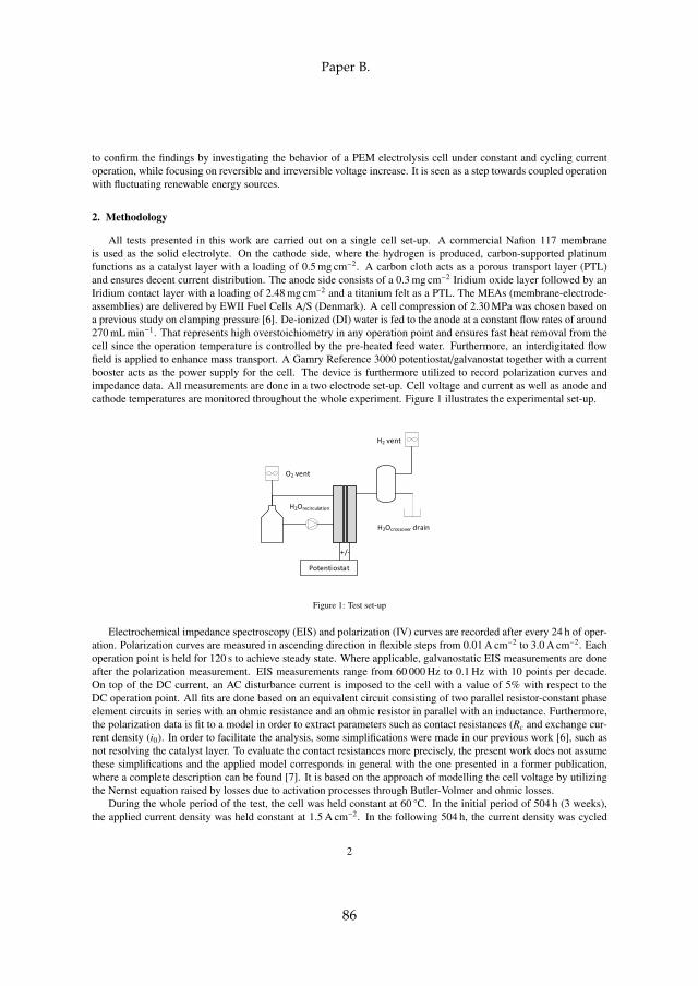
to confirm the findings by investigating the behavior of a PEM electrolysis cell under constant and cycling currentoperation, while focusing on reversible and irreversible voltage increase. It is seen as a step towards coupled operationwith fluctuating renewable energy sources.
2. Methodology
All tests presented in this work are carried out on a single cell set-up. A commercial Nafion 117 membraneis used as the solid electrolyte. On the cathode side, where the hydrogen is produced, carbon-supported platinumfunctions as a catalyst layer with a loading of 0.5 mg cm−2. A carbon cloth acts as a porous transport layer (PTL)and ensures decent current distribution. The anode side consists of a 0.3 mg cm−2 Iridium oxide layer followed by anIridium contact layer with a loading of 2.48 mg cm−2 and a titanium felt as a PTL. The MEAs (membrane-electrode-assemblies) are delivered by EWII Fuel Cells A/S (Denmark). A cell compression of 2.30 MPa was chosen based ona previous study on clamping pressure [6]. De-ionized (DI) water is fed to the anode at a constant flow rates of around270 mL min−1. That represents high overstoichiometry in any operation point and ensures fast heat removal from thecell since the operation temperature is controlled by the pre-heated feed water. Furthermore, an interdigitated flowfield is applied to enhance mass transport. A Gamry Reference 3000 potentiostat/galvanostat together with a currentbooster acts as the power supply for the cell. The device is furthermore utilized to record polarization curves andimpedance data. All measurements are done in a two electrode set-up. Cell voltage and current as well as anode andcathode temperatures are monitored throughout the whole experiment. Figure 1 illustrates the experimental set-up.
H2Ocrossover drain
H2 vent
H2Orecirculation
O2 vent
Potentiostat
+/-
Figure 1: Test set-up
Electrochemical impedance spectroscopy (EIS) and polarization (IV) curves are recorded after every 24 h of oper-ation. Polarization curves are measured in ascending direction in flexible steps from 0.01 A cm−2 to 3.0 A cm−2. Eachoperation point is held for 120 s to achieve steady state. Where applicable, galvanostatic EIS measurements are doneafter the polarization measurement. EIS measurements range from 60 000 Hz to 0.1 Hz with 10 points per decade.On top of the DC current, an AC disturbance current is imposed to the cell with a value of 5% with respect to theDC operation point. All fits are done based on an equivalent circuit consisting of two parallel resistor-constant phaseelement circuits in series with an ohmic resistance and an ohmic resistor in parallel with an inductance. Furthermore,the polarization data is fit to a model in order to extract parameters such as contact resistances (Rc and exchange cur-rent density (i0). In order to facilitate the analysis, some simplifications were made in our previous work [6], such asnot resolving the catalyst layer. To evaluate the contact resistances more precisely, the present work does not assumethese simplifications and the applied model corresponds in general with the one presented in a former publication,where a complete description can be found [7]. It is based on the approach of modelling the cell voltage by utilizingthe Nernst equation raised by losses due to activation processes through Butler-Volmer and ohmic losses.
During the whole period of the test, the cell was held constant at 60 C. In the initial period of 504 h (3 weeks),the applied current density was held constant at 1.5 A cm−2. In the following 504 h, the current density was cycled
2
Paper B.
86
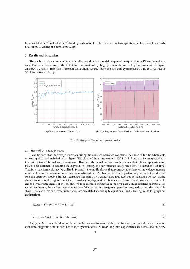
between 1.0 A cm−2 and 2.0 A cm−2, holding each value for 1 h. Between the two operation modes, the cell was onlyinterrupted to change the automated script.
3. Results and Discussion
The analysis is based on the voltage profile over time, and model-supported interpretation of IV and impedancedata. For the whole period of the test at both constant and cycling operation, the cell voltage was monitored. Figure2a shows the whole time span of the constant current period, figure 2b shows the cycling period only as an extract of200 h for better visibility.
0 50 100 150 200 250 300 350 400 450 500
runtime at operation mode /h
1.4
1.5
1.6
1.7
1.8
1.9
2
2.1
2.2
2.3
2.4
i /A
*cm
-2, V
/V
iVfit: y=109.8uV/h*x+2.047
(a) Constant current, 0 h to 504 h
200 220 240 260 280 300 320 340 360 380 400
runtime at operation mode /h
1
1.2
1.4
1.6
1.8
2
2.2
2.4
i /A
*cm
-2, V
/V
iV (60°C)
(b) Cycling, extract from 200 h to 400 h for better visibility
Figure 2: Voltage profiles for both operation modes
3.1. Reversible Voltage IncreaseIt can be seen that the voltage increases during the constant operation over time. A linear fit for the whole data
set was applied and included in the figure. The slope of the fitting curve is 109.8 µV h−1 and can be interpreted as afirst estimation of the voltage increase rate. However, the actual voltage profile reveals, that a linear approximationmay not be sufficient to describe the degradation. Firstly, the performance decay rate seems to decrease over time.That is, a logarithmic fit may be utilized. Secondly, the profile shows that a considerable share of the voltage increaseis reversible and is recovered after each characterization. At this point, it is important to point out, that also theconstant operation mode is in fact interrupted frequently by a characterization. Last but not least, the voltage profilealone cannot reveal insights about the the underlying degradation phenomena. Figure 3b illustrates the reversibleand the irreversible shares of the absolute voltage increase during the respective past 24 h at constant operation. Asmentioned before, the total voltage increase over 24 h decreases throughout operation time, and so does the reversibleshare. The reversible and irreversible shares are calculated according to equations 1 and 2 (see figure 3a for graphicalexplanation).
Vrev(t) = V(t, end) − V(t + 1, start) (1)
Virrev(t) = V(t + 1, start) − V(t, start) (2)
As figure 3c shows, the share of the reversible voltage increase of the total increase does not show a clear trendover time, suggesting that it does not change systematically. Similar long term experiments are scarce and only few
3
87
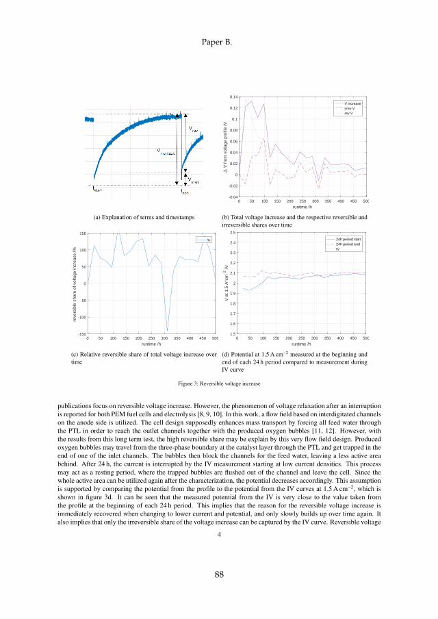
(a) Explanation of terms and timestamps
0 50 100 150 200 250 300 350 400 450 500
runtime /h
-0.04
-0.02
0
0.02
0.04
0.06
0.08
0.1
0.12
0.14
V fr
om v
olta
ge p
rofil
e /V
V increaseirrev Vrev V
(b) Total voltage increase and the respective reversible andirreversible shares over time
0 50 100 150 200 250 300 350 400 450 500
runtime /h
-150
-100
-50
0
50
100
150
reve
rsib
le s
hare
of v
olta
ge in
crea
se /%
%
(c) Relative reversible share of total voltage increase overtime
0 50 100 150 200 250 300 350 400 450 500
runtime /h
1.5
1.6
1.7
1.8
1.9
2
2.1
2.2
2.3
2.4
2.5
V a
t 1.5
A*c
m-2
/V
24h period start24h period endIV
(d) Potential at 1.5 A cm−2 measured at the beginning andend of each 24 h period compared to measurement duringIV curve
Figure 3: Reversible voltage increase
publications focus on reversible voltage increase. However, the phenomenon of voltage relaxation after an interruptionis reported for both PEM fuel cells and electrolysis [8, 9, 10]. In this work, a flow field based on interdigitated channelson the anode side is utilized. The cell design supposedly enhances mass transport by forcing all feed water throughthe PTL in order to reach the outlet channels together with the produced oxygen bubbles [11, 12]. However, withthe results from this long term test, the high reversible share may be explain by this very flow field design. Producedoxygen bubbles may travel from the three-phase boundary at the catalyst layer through the PTL and get trapped in theend of one of the inlet channels. The bubbles then block the channels for the feed water, leaving a less active areabehind. After 24 h, the current is interrupted by the IV measurement starting at low current densities. This processmay act as a resting period, where the trapped bubbles are flushed out of the channel and leave the cell. Since thewhole active area can be utilized again after the characterization, the potential decreases accordingly. This assumptionis supported by comparing the potential from the profile to the potential from the IV curves at 1.5 A cm−2, which isshown in figure 3d. It can be seen that the measured potential from the IV is very close to the value taken fromthe profile at the beginning of each 24 h period. This implies that the reason for the reversible voltage increase isimmediately recovered when changing to lower current and potential, and only slowly builds up over time again. Italso implies that only the irreversible share of the voltage increase can be captured by the IV curve. Reversible voltage
4
Paper B.
88
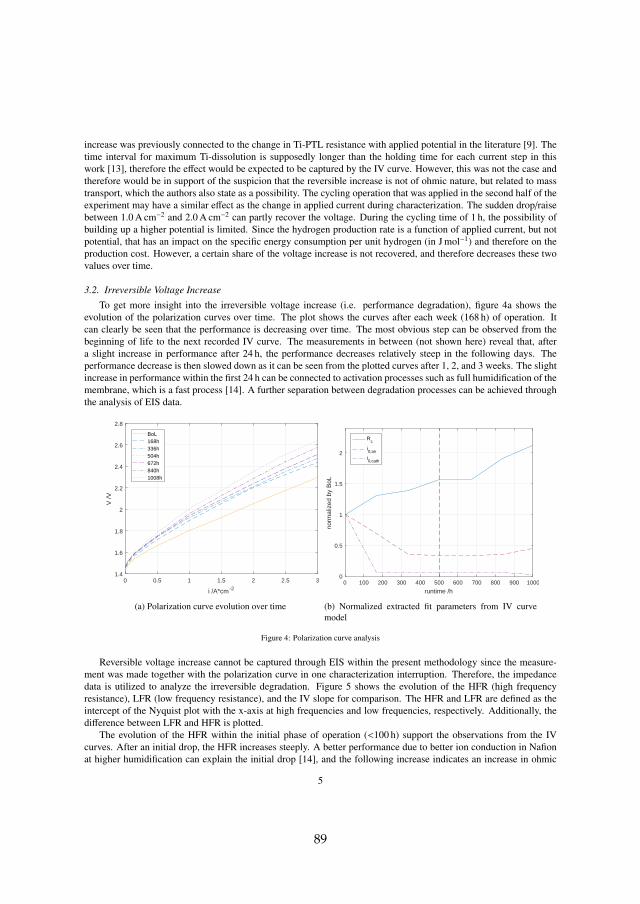
increase was previously connected to the change in Ti-PTL resistance with applied potential in the literature [9]. Thetime interval for maximum Ti-dissolution is supposedly longer than the holding time for each current step in thiswork [13], therefore the effect would be expected to be captured by the IV curve. However, this was not the case andtherefore would be in support of the suspicion that the reversible increase is not of ohmic nature, but related to masstransport, which the authors also state as a possibility. The cycling operation that was applied in the second half of theexperiment may have a similar effect as the change in applied current during characterization. The sudden drop/raisebetween 1.0 A cm−2 and 2.0 A cm−2 can partly recover the voltage. During the cycling time of 1 h, the possibility ofbuilding up a higher potential is limited. Since the hydrogen production rate is a function of applied current, but notpotential, that has an impact on the specific energy consumption per unit hydrogen (in J mol−1) and therefore on theproduction cost. However, a certain share of the voltage increase is not recovered, and therefore decreases these twovalues over time.
3.2. Irreversible Voltage Increase
To get more insight into the irreversible voltage increase (i.e. performance degradation), figure 4a shows theevolution of the polarization curves over time. The plot shows the curves after each week (168 h) of operation. Itcan clearly be seen that the performance is decreasing over time. The most obvious step can be observed from thebeginning of life to the next recorded IV curve. The measurements in between (not shown here) reveal that, aftera slight increase in performance after 24 h, the performance decreases relatively steep in the following days. Theperformance decrease is then slowed down as it can be seen from the plotted curves after 1, 2, and 3 weeks. The slightincrease in performance within the first 24 h can be connected to activation processes such as full humidification of themembrane, which is a fast process [14]. A further separation between degradation processes can be achieved throughthe analysis of EIS data.
0 0.5 1 1.5 2 2.5 3
i /A*cm -2
1.4
1.6
1.8
2
2.2
2.4
2.6
2.8
V /V
BoL168h336h504h672h840h1008h
(a) Polarization curve evolution over time
0 100 200 300 400 500 600 700 800 900 1000
runtime /h
0
0.5
1
1.5
2
norm
aliz
ed b
y B
oL
Rc
i0,an
i0,cath
(b) Normalized extracted fit parameters from IV curvemodel
Figure 4: Polarization curve analysis
Reversible voltage increase cannot be captured through EIS within the present methodology since the measure-ment was made together with the polarization curve in one characterization interruption. Therefore, the impedancedata is utilized to analyze the irreversible degradation. Figure 5 shows the evolution of the HFR (high frequencyresistance), LFR (low frequency resistance), and the IV slope for comparison. The HFR and LFR are defined as theintercept of the Nyquist plot with the x-axis at high frequencies and low frequencies, respectively. Additionally, thedifference between LFR and HFR is plotted.
The evolution of the HFR within the initial phase of operation (<100 h) support the observations from the IVcurves. After an initial drop, the HFR increases steeply. A better performance due to better ion conduction in Nafionat higher humidification can explain the initial drop [14], and the following increase indicates an increase in ohmic
5
89
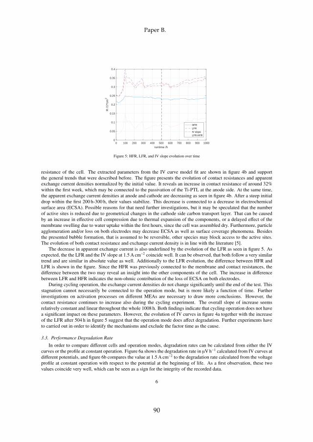
0 100 200 300 400 500 600 700 800 900 1000
runtime /h
0
0.05
0.1
0.15
0.2
0.25
0.3
0.35
0.4
R /
*cm
2
HFRLFRIV slopeLFR-HFR
Figure 5: HFR, LFR, and IV slope evolution over time
resistance of the cell. The extracted parameters from the IV curve model fit are shown in figure 4b and supportthe general trends that were described before. The figure presents the evolution of contact resistances and apparentexchange current densities normalized by the initial value. It reveals an increase in contact resistance of around 32%within the first week, which may be connected to the passivation of the Ti-PTL at the anode side. At the same time,the apparent exchange current densities at anode and cathode are decreasing as seen in figure 4b. After a steep initialdrop within the first 200 h-300 h, their values stabilize. This decrease is connected to a decrease in electrochemicalsurface area (ECSA). Possible reasons for that need further investigations, but it may be speculated that the numberof active sites is reduced due to geometrical changes in the cathode side carbon transport layer. That can be causedby an increase in effective cell compression due to thermal expansion of the components, or a delayed effect of themembrane swelling due to water uptake within the first hours, since the cell was assembled dry. Furthermore, particleagglomeration and/or loss on both electrodes may decrease ECSA as well as surface coverage phenomena. Besidesthe presented bubble formation, that is assumed to be reversible, other species may block access to the active sites.The evolution of both contact resistance and exchange current density is in line with the literature [5].
The decrease in apparent exchange current is also underlined by the evolution of the LFR as seen in figure 5. Asexpected, the the LFR and the IV slope at 1.5 A cm−2 coincide well. It can be observed, that both follow a very similartrend and are similar in absolute value as well. Additionally to the LFR evolution, the difference between HFR andLFR is shown in the figure. Since the HFR was previously connected to the membrane and contact resistances, thedifference between the two may reveal an insight into the other components of the cell. The increase in differencebetween LFR and HFR indicates the non-ohmic contribution of the loss of ECSA on both electrodes.
During cycling operation, the exchange current densities do not change significantly until the end of the test. Thisstagnation cannot necessarily be connected to the operation mode, but is more likely a function of time. Furtherinvestigations on activation processes on different MEAs are necessary to draw more conclusions. However, thecontact resistance continues to increase also during the cycling experiment. The overall slope of increase seemsrelatively constant and linear throughout the whole 1008 h. Both findings indicate that cycling operation does not havea significant impact on these parameters. However, the evolution of IV curves in figure 4a together with the increaseof the LFR after 504 h in figure 5 suggest that the operation mode does affect degradation. Further experiments haveto carried out in order to identify the mechanisms and exclude the factor time as the cause.
3.3. Performance Degradation Rate
In order to compare different cells and operation modes, degradation rates can be calculated from either the IVcurves or the profile at constant operation. Figure 6a shows the degradation rate in µV h−1 calculated from IV curves atdifferent potentials, and figure 6b compares the value at 1.5 A cm−2 to the degradation rate calculated from the voltageprofile at constant operation with respect to the potential at the beginning of life. As a first observation, these twovalues coincide very well, which can be seen as a sign for the integrity of the recorded data.
6
Paper B.
90
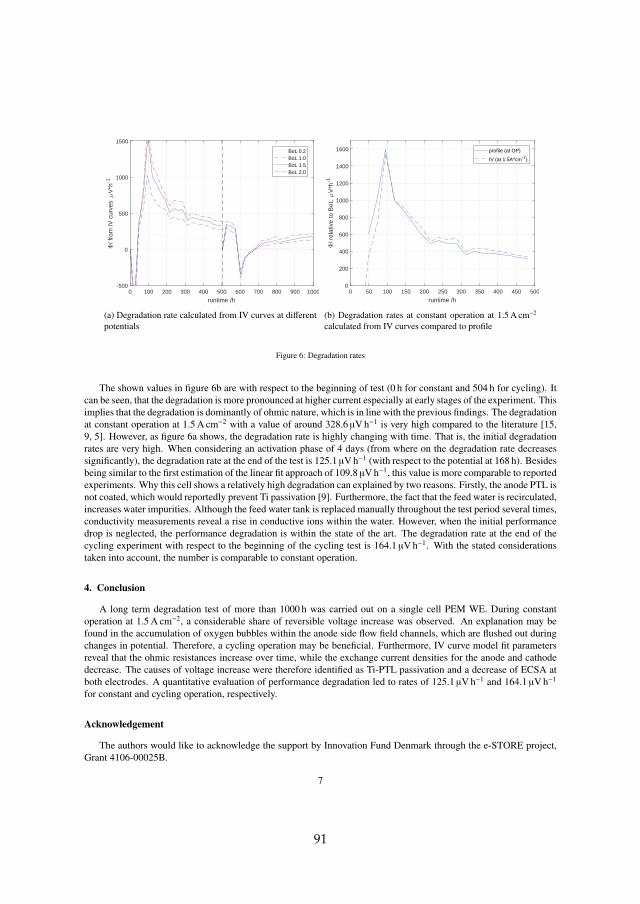
0 100 200 300 400 500 600 700 800 900 1000
runtime /h
-500
0
500
1000
1500
/ fro
m IV
cur
ves
V*h
-1
BoL 0.2BoL 1.0BoL 1.5BoL 2.0
(a) Degradation rate calculated from IV curves at differentpotentials
0 50 100 150 200 250 300 350 400 450 500
runtime /h
0
200
400
600
800
1000
1200
1400
1600
/ rel
ativ
e to
BoL
V
*h-1
profile (at OP)
IV (at 1.5A*cm-2)
(b) Degradation rates at constant operation at 1.5 A cm−2
calculated from IV curves compared to profile
Figure 6: Degradation rates
The shown values in figure 6b are with respect to the beginning of test (0 h for constant and 504 h for cycling). Itcan be seen, that the degradation is more pronounced at higher current especially at early stages of the experiment. Thisimplies that the degradation is dominantly of ohmic nature, which is in line with the previous findings. The degradationat constant operation at 1.5 A cm−2 with a value of around 328.6 µV h−1 is very high compared to the literature [15,9, 5]. However, as figure 6a shows, the degradation rate is highly changing with time. That is, the initial degradationrates are very high. When considering an activation phase of 4 days (from where on the degradation rate decreasessignificantly), the degradation rate at the end of the test is 125.1 µV h−1 (with respect to the potential at 168 h). Besidesbeing similar to the first estimation of the linear fit approach of 109.8 µV h−1, this value is more comparable to reportedexperiments. Why this cell shows a relatively high degradation can explained by two reasons. Firstly, the anode PTL isnot coated, which would reportedly prevent Ti passivation [9]. Furthermore, the fact that the feed water is recirculated,increases water impurities. Although the feed water tank is replaced manually throughout the test period several times,conductivity measurements reveal a rise in conductive ions within the water. However, when the initial performancedrop is neglected, the performance degradation is within the state of the art. The degradation rate at the end of thecycling experiment with respect to the beginning of the cycling test is 164.1 µV h−1. With the stated considerationstaken into account, the number is comparable to constant operation.
4. Conclusion
A long term degradation test of more than 1000 h was carried out on a single cell PEM WE. During constantoperation at 1.5 A cm−2, a considerable share of reversible voltage increase was observed. An explanation may befound in the accumulation of oxygen bubbles within the anode side flow field channels, which are flushed out duringchanges in potential. Therefore, a cycling operation may be beneficial. Furthermore, IV curve model fit parametersreveal that the ohmic resistances increase over time, while the exchange current densities for the anode and cathodedecrease. The causes of voltage increase were therefore identified as Ti-PTL passivation and a decrease of ECSA atboth electrodes. A quantitative evaluation of performance degradation led to rates of 125.1 µV h−1 and 164.1 µV h−1
for constant and cycling operation, respectively.
Acknowledgement
The authors would like to acknowledge the support by Innovation Fund Denmark through the e-STORE project,Grant 4106-00025B.
7
91
References
[1] A. Godula-Jopek, Hydrogen Production by Electrolysis, Wiley-VCH, 2015.[2] B. Bensmann, R. Hanke-Rauschenbach, I. K. Pena Arias, K. Sundmacher, Energetic evaluation of high pressure PEM electrolyzer systems
for intermediate storage of renewable energies, Electrochimica Acta 110 (2013) 570–580. doi:10.1016/j.electacta.2013.05.102.[3] E. Anderson, K. Ayers, C. Capuano, R & D Focus Areas Based on 60 , 000 hr Life PEM Water Electrolysis Stack Experience p Proton OnSite
Manufacturer of packaged products , systems, First International Workshop on Durability and Degradation Issues in PEM Electrolysis Cellsand its Components (March).
[4] F. Fouda-Onana, M. Chandesris, V. Medeau, S. Chelghoum, D. Thoby, N. Guillet, Investigation on the degradation of MEAs for PEMwater electrolysers part I: Effects of testing conditions on MEA performances and membrane properties, International Journal of HydrogenEnergy (41) (2016) 16627–16636. doi:10.1016/j.ijhydene.2016.07.125.
[5] C. Rakousky, U. Reimer, K. Wippermann, S. Kuhri, M. Carmo, W. Lueke, D. Stolten, Polymer electrolyte membrane water electrolysis: Re-straining degradation in the presence of fluctuating power, Journal of Power Sources 342 (2017) 38–47. doi:10.1016/j.jpowsour.2016.11.118.URL http://dx.doi.org/10.1016/j.jpowsour.2016.11.118
[6] S. H. Frensch, A. C. Olesen, S. S. Araya, S. K. Kær, Model-supported characterization of a PEM water electrolysis cell for the effect ofcompression, Electrochimica Actadoi:10.1016/j.electacta.2018.01.040.URL https://doi.org/10.1016/j.electacta.2018.01.040
[7] A. C. Olesen, S. K. Kær, The Effect of PFSA Membrane Compression on the Predicted Performance of a High Pressure PEM ElectrolysisCell, ECS Transactions 68 (3) (2015) 99–116. doi:10.1149/06803.0099ecst.
[8] M. Chandesris, T. Jahnke, M. Zago, T. A. Aarhaug, P. Schott, M. Baum, Investigation of permanent and reversible degradations in PEMFCand DMFC stationary applications using statistical and modelling tools, in: Modval13, 2016, p. 621216.
[9] C. Rakousky, U. Reimer, K. Wippermann, M. Carmo, W. Lueke, D. Stolten, An analysis of degradation phenomena in polymer electrolytemembrane water electrolysis, Journal of Power Sources 326 (2016) 120–128. doi:http://dx.doi.org/10.1016/j.jpowsour.2016.06.082.URL http://www.sciencedirect.com/science/article/pii/S0378775316307844
[10] W. Schmittinger, A. Vahidi, A review of the main parameters influencing long-term performance and durability of PEM fuel cells, Journal ofPower Sources 180 (2008) 1–14. doi:10.1016/j.jpowsour.2008.01.070.
[11] T. V. Nguyen, A gas distributor design for proton-exchange-membrane fuel cells, Journal of The Electrochemical Society 143 (5) (1996)L103–L105. doi:Doi 10.1149/1.1836666.
[12] D. L. Wood, Y. S. Yi, T. V. Nguyen, Effect of direct liquid water injection and interdigitated flow field on the performance of proton exchangemembrane fuel cells, Electrochimica Acta 43 (24) (1998) 3795–3809. doi:10.1016/S0013-4686(98)00139-X.
[13] S. Cherevko, T. Reier, A. R. Zeradjanin, Z. Pawolek, P. Strasser, K. J. Mayrhofer, Stability of nanostructured iridium ox-ide electrocatalysts during oxygen evolution reaction in acidic environment, Electrochemistry Communications 48 (2014) 81–85.doi:10.1016/j.elecom.2014.08.027.URL http://dx.doi.org/10.1016/j.elecom.2014.08.027
[14] T. a. Zawodzinski, Water Uptake by and Transport Through Nafion® 117 Membranes, Journal of The Electrochemical Society 140 (4) (1993)1041. doi:10.1149/1.2056194.
[15] P. Lettenmeier, R. Wang, R. Abouatallah, S. Helmly, T. Morawietz, R. Hiesgen, S. Kolb, F. Burggraf, J. Kallo, A. S. Gago, K. A. Friedrich,Durable Membrane Electrode Assemblies for Proton Exchange Membrane Electrolyzer Systems Operating at High Current Densities, Elec-trochimica Acta 210 (2016) 502–511. doi:10.1016/j.electacta.2016.04.164.URL http://dx.doi.org/10.1016/j.electacta.2016.04.164
8
Paper B.
92
Paper C
Influence of the OperationMode on PEM WaterElectrolysis Degradation
Steffen Henrik Frensch, Frédéric Fouda-Onana, GuillaumeSerre, Dominique Thoby, Samuel Simon Araya, Søren Knudsen
Kær.
The paper has been submitted to theInternational Journal of Hydrogen Energy.
93

submitted to an Elsevier Ltd. journal
Influence of the Operation Mode on PEM Water Electrolysis Degradation
Steffen Henrik Frenscha,∗, Frederic Fouda-Onanab, Guillaume Serreb, Dominique Thobyb, Samuel Simon Arayaa,Søren Knudsen Kæra
aAalborg University, Department of Energy Technology, Pontoppidanstræde 111, 9220 Aalborg Øst, DenmarkbCEA, LITEN, DEHT, F-38054, Grenoble, France
Abstract
Since realistic operation scenarios for polymer electrolyte membrane water electrolysis (PEM WE) systems may bedynamic, this study compares the performance over time for seven different operation modes. Besides the effect oftemperature, constant and dynamic current profiles were investigated, including cycling operation and the simulationof a solar profile. It was found that fast current switches improved the overall cell performance over the test periodof 500 h. The major cause for this was a decrease in total ohmic resistance, which was also observed during thebreak-in phase preceding the experiments. This decrease can partly be explained by membrane thinning and partlyby an improvement in contacts between the components. Dynamic operation led to more severe fluoride emissionfrom the catalyst binder, which improved the performance in terms of cell potential. However, it could be a concernfor long term degradation as membrane thinning promotes higher gas crossover. All other operation modes on theother hand suffered from an increase in total ohmic resistance, leading to an overall performance decrease. This wasconnected to the passivation of Ti components. Higher temperature was found to be advantageous for performance,but disadvantageous in terms of both membrane thinning and passivation processes.
Keywords: PEM water electrolysis aging, Membrane Degradation, Dynamic operation mode, Durability, Break-in
1. Introduction
Hydrogen may play an important role in future energy systems. With the transition from fossil fuels to fluctuatingenergy sources such as solar and wind comes an increase in fluctuation of power input. Due to its multiple appli-cations in this context, hydrogen production through polymer electrolyte membrane water electrolysis (PEM WE)is a subject of increasing attention [1]. The technology may be utilized for energy storage by producing hydrogenfor a later use to convert it back into electrical energy or thermal energy. Besides using gaseous hydrogen directlyfor example in PEM fuel cells (FC), it can also be part of power-to-x systems including syngas or liquid fuels suchas methanol [2, 3]. Furthermore, due to certain advantages, PEM electrolysis may take over grid services such asfrequency stabilization [1], that were previously provided by conventional thermal turbines through their inertia. Lastbut not least, water electrolysis presents an alternative to natural gas reforming for industrial hydrogen production thatis potentially CO2 neutral.
Although the PEM technology for both fuel cells and electrolysis is well researched, a wide market implementationis not yet observed. One of the biggest challenges is the high cost of production, which has to be addressed both bylowering material cost and by extending the useful lifetime of the system. An increasing amount of literature isavailable on the topic, but especially degradation under dynamic operation has a demand for more research. The mostcomprehensive work with the focus on dynamic operation can be found in [4], where the authors compare differentoperation modes in terms of degradation rates. The work includes the contributions of anode and cathode through
∗Corresponding authorEmail addresses: [email protected] (Steffen Henrik Frensch), [email protected] (Frederic Fouda-Onana),
[email protected] (Guillaume Serre), [email protected] (Dominique Thoby), [email protected] (Samuel Simon Araya),[email protected] (Søren Knudsen Kær)
Preprint submitted to International Journal of Hydrogen Energy November 8, 2018
95
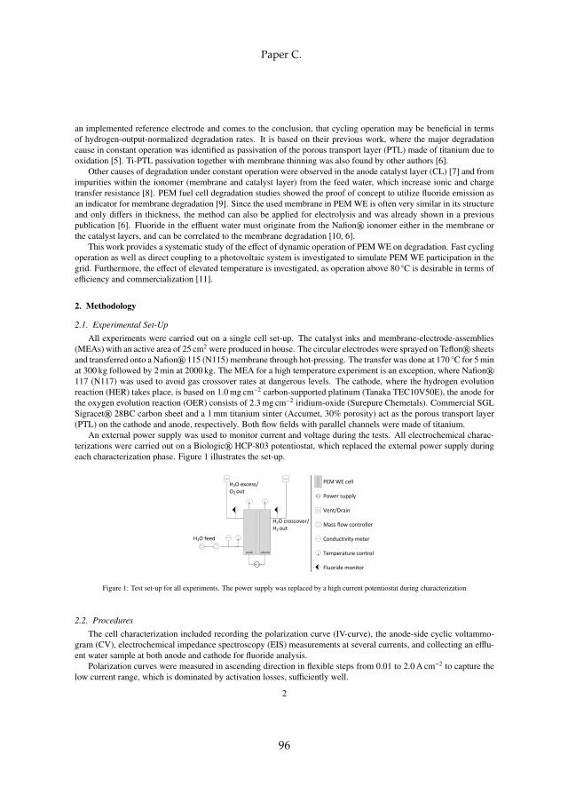
an implemented reference electrode and comes to the conclusion, that cycling operation may be beneficial in termsof hydrogen-output-normalized degradation rates. It is based on their previous work, where the major degradationcause in constant operation was identified as passivation of the porous transport layer (PTL) made of titanium due tooxidation [5]. Ti-PTL passivation together with membrane thinning was also found by other authors [6].
Other causes of degradation under constant operation were observed in the anode catalyst layer (CL) [7] and fromimpurities within the ionomer (membrane and catalyst layer) from the feed water, which increase ionic and chargetransfer resistance [8]. PEM fuel cell degradation studies showed the proof of concept to utilize fluoride emission asan indicator for membrane degradation [9]. Since the used membrane in PEM WE is often very similar in its structureand only differs in thickness, the method can also be applied for electrolysis and was already shown in a previouspublication [6]. Fluoride in the effluent water must originate from the Nafion® ionomer either in the membrane orthe catalyst layers, and can be correlated to the membrane degradation [10, 6].
This work provides a systematic study of the effect of dynamic operation of PEM WE on degradation. Fast cyclingoperation as well as direct coupling to a photovoltaic system is investigated to simulate PEM WE participation in thegrid. Furthermore, the effect of elevated temperature is investigated, as operation above 80 C is desirable in terms ofefficiency and commercialization [11].
2. Methodology
2.1. Experimental Set-Up
All experiments were carried out on a single cell set-up. The catalyst inks and membrane-electrode-assemblies(MEAs) with an active area of 25 cm2 were produced in house. The circular electrodes were sprayed on Teflon® sheetsand transferred onto a Nafion® 115 (N115) membrane through hot-pressing. The transfer was done at 170 C for 5 minat 300 kg followed by 2 min at 2000 kg. The MEA for a high temperature experiment is an exception, where Nafion®117 (N117) was used to avoid gas crossover rates at dangerous levels. The cathode, where the hydrogen evolutionreaction (HER) takes place, is based on 1.0 mg cm−2 carbon-supported platinum (Tanaka TEC10V50E), the anode forthe oxygen evolution reaction (OER) consists of 2.3 mg cm−2 iridium-oxide (Surepure Chemetals). Commercial SGLSigracet® 28BC carbon sheet and a 1 mm titanium sinter (Accumet, 30% porosity) act as the porous transport layer(PTL) on the cathode and anode, respectively. Both flow fields with parallel channels were made of titanium.
An external power supply was used to monitor current and voltage during the tests. All electrochemical charac-terizations were carried out on a Biologic® HCP-803 potentiostat, which replaced the external power supply duringeach characterization phase. Figure 1 illustrates the set-up.
anode cathode
H2O crossover/ H2 out
H2O feed
H2O excess/ O2 out
PEM WE cell
Power supply
Vent/Drain
Mass flow controller
Conductivity meter
Temperature control
Fluoride monitor
Figure 1: Test set-up for all experiments. The power supply was replaced by a high current potentiostat during characterization
2.2. Procedures
The cell characterization included recording the polarization curve (IV-curve), the anode-side cyclic voltammo-gram (CV), electrochemical impedance spectroscopy (EIS) measurements at several currents, and collecting an efflu-ent water sample at both anode and cathode for fluoride analysis.
Polarization curves were measured in ascending direction in flexible steps from 0.01 to 2.0 A cm−2 to capture thelow current range, which is dominated by activation losses, sufficiently well.
2
Paper C.
96

This was followed by galvanostatic EIS measurements at 0.1, 0.5, 1.0, 1.5, and 2.0 A cm−2. The frequency rangewas set to 60 000 Hz - 0.1 Hz, with 10 points per decade and an AC amplitude of 5% of the value of the DC operationpoint. For this work, the impedance data is used to extract the intercepts with the x-axis in the Nyquist representationat high and low frequency. The high frequency intercept (HFR) represents all ohmic resistances of the cell assembly,whereas the low frequency intercept (LFR) represents the polarization resistance.
During the CV measurements, the cathode side was flushed with hydrogen gas, while the water flow was keptconstant at the anode. Measurements with scan rates of 300 and 50 mV s−1 were recorded. Furthermore, a sampleof effluent water at anode and cathode outlets at 0.3 A cm−2 was captured for each point of characterization. As atrade-off between the need for capturing steady state ion concentrations and short collection time to exclude capturingtransients, the effluent water was collected for 150 s at the anode and 1 h at the cathode side. The samples were thenanalyzed in an ion chromatograph (Thermo Scientific DIONEX® ICS 2100) for fluoride content.
Finally, the MEAs were investigated ex-situ under a ZEIS LEO 1530 scanning electron microscope (SEM). Allsamples were taken from the same spot in the middle of the MEA, put into a resin and polished for examination.
The tests were run at atmospheric pressure with a constant feed water flow rate of 500 mL h−1 without recircu-lation. The feed water was preheated to the operation temperature and the conductivity was monitored throughoutthe whole test to ensure sufficient quality of 18.2 MΩ · cm. Additionally, heater pads on both sides were installedfor a homogeneous temperature distribution within the cell. Each experiment was run for at least 500 h. Table 1summarizes the investigated operation modes. The parameter of interest besides temperature was the current profile.Therefore, one constant and three dynamic current profiles were tested. The solar profile was constructed from dataof a real photovoltaic system over 16 h, where the the mean value was around 1.0 A cm−2 and the dwell time 60 s.The periods of the two current cycling profiles, 100 s and 10 s, were extracted by a Fourier transformation of the solarprofile. Although no clear dominant frequency was identified, two broad peaks at the highest frequencies were chosenas highly dynamic operation is simulated.
# operation mode operation point temperature experiment name1 constant current 2.0 A cm−2 80 C cc2 constant voltage 2.0 V 60 C T603 constant voltage 2.0 V 80 C T804 constant voltage 2.0 V 90 C T905 cycling current 0–2.0 A cm−2, 100 s dwell time 80 C cyc100s
6 cycling current 0–2.0 A cm−2, 10 s dwell time 80 C cyc10s
7 dynamic current 0–2.0 A cm−2, 60 s dwell time,solar profile
80 C solar
Table 1: Investigated operation modes. Each experiment was carried out on a fresh cell assembly after break-in for at least 500 h
3. Results and discussion
3.1. Break-in phase monitoringAll cells went through the same break-in phase according to the procedure seen in figure 2a. The procedure
includes current steps at lower and higher frequencies, and periods of constant current. One cycle lasts around 40 minand is repeated for around 60 h. To get more insight into the involved processes, the break-in phase of experimentsolar was monitored, including short EIS measurements at the indicated points. The parameters were set to haveas little impact on the actual procedure as possible. Furthermore, the anode side CV was recorded before and afterbreak-in.
Break-in may generally be assumed to make more active sites available [12]. This could be achieved by washingimpurities within the components that originate from the manufacturing and assembly process. In fact, the recordedanode side CVs before and after break-in indicate an increase in active sites with around 6% increase in charge at50 mV s−1 as seen in figure 2d. When looking at the evolution of potentials and EIS data, a clear impact over time isvisible. As seen in figure 2b, the potential at 2.0 A cm−2 drops considerably from around 2.07 V after the first cycle to1.88 V after 21 cycles and a little further down to 1.84 V just before the break-in was terminated after 83 cycles. At
3
97
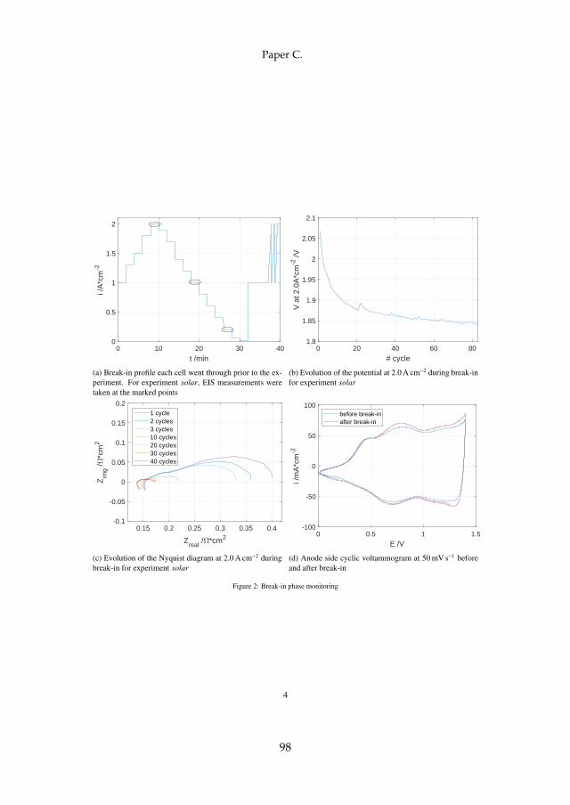
0 10 20 30 40
t /min
0
0.5
1
1.5
2
i /A
*cm
-2
(a) Break-in profile each cell went through prior to the ex-periment. For experiment solar, EIS measurements weretaken at the marked points
0 20 40 60 80
# cycle
1.8
1.85
1.9
1.95
2
2.05
2.1
V a
t 2.0
A*c
m-2
/V
(b) Evolution of the potential at 2.0 A cm−2 during break-infor experiment solar
0.15 0.2 0.25 0.3 0.35 0.4
Zreal
/ *cm2
-0.1
-0.05
0
0.05
0.1
0.15
0.2
Zim
g /
*cm
2
1 cycle2 cycles3 cycles10 cycles20 cycles30 cycles40 cycles
(c) Evolution of the Nyquist diagram at 2.0 A cm−2 duringbreak-in for experiment solar
0 0.5 1 1.5
E /V
-100
-50
0
50
100
i /m
A*c
m-2
before break-inafter break-in
(d) Anode side cyclic voltammogram at 50 mV s−1 beforeand after break-in
Figure 2: Break-in phase monitoring
4
Paper C.
98
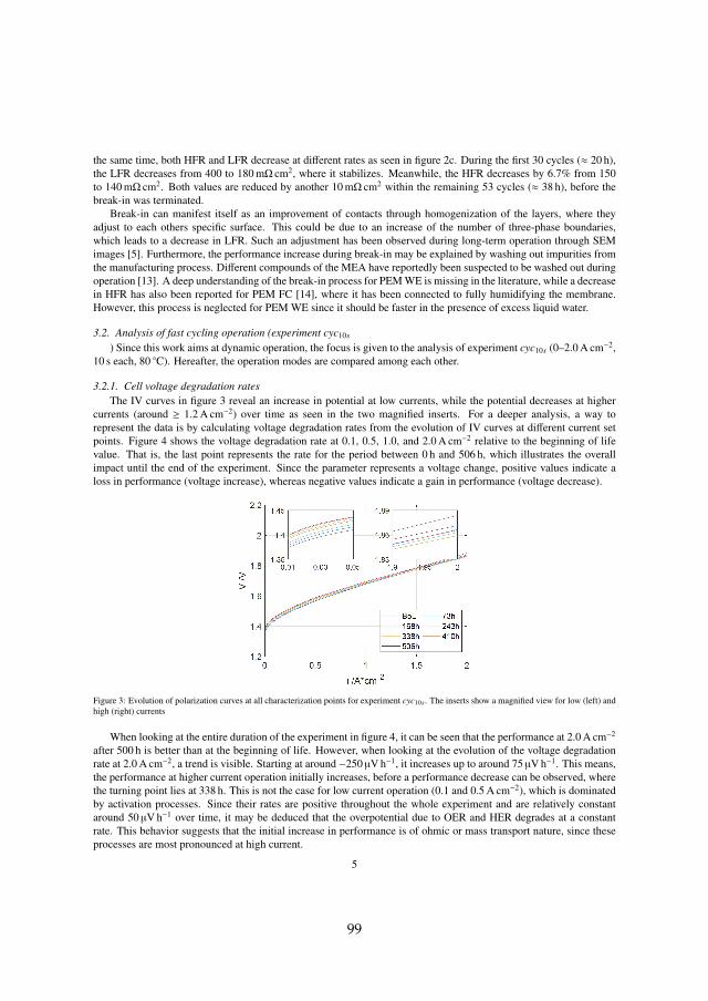
the same time, both HFR and LFR decrease at different rates as seen in figure 2c. During the first 30 cycles (≈ 20 h),the LFR decreases from 400 to 180 mΩ cm2, where it stabilizes. Meanwhile, the HFR decreases by 6.7% from 150to 140 mΩ cm2. Both values are reduced by another 10 mΩ cm2 within the remaining 53 cycles (≈ 38 h), before thebreak-in was terminated.
Break-in can manifest itself as an improvement of contacts through homogenization of the layers, where theyadjust to each others specific surface. This could be due to an increase of the number of three-phase boundaries,which leads to a decrease in LFR. Such an adjustment has been observed during long-term operation through SEMimages [5]. Furthermore, the performance increase during break-in may be explained by washing out impurities fromthe manufacturing process. Different compounds of the MEA have reportedly been suspected to be washed out duringoperation [13]. A deep understanding of the break-in process for PEM WE is missing in the literature, while a decreasein HFR has also been reported for PEM FC [14], where it has been connected to fully humidifying the membrane.However, this process is neglected for PEM WE since it should be faster in the presence of excess liquid water.
3.2. Analysis of fast cycling operation (experiment cyc10s
) Since this work aims at dynamic operation, the focus is given to the analysis of experiment cyc10s (0–2.0 A cm−2,10 s each, 80 C). Hereafter, the operation modes are compared among each other.
3.2.1. Cell voltage degradation ratesThe IV curves in figure 3 reveal an increase in potential at low currents, while the potential decreases at higher
currents (around ≥ 1.2 A cm−2) over time as seen in the two magnified inserts. For a deeper analysis, a way torepresent the data is by calculating voltage degradation rates from the evolution of IV curves at different current setpoints. Figure 4 shows the voltage degradation rate at 0.1, 0.5, 1.0, and 2.0 A cm−2 relative to the beginning of lifevalue. That is, the last point represents the rate for the period between 0 h and 506 h, which illustrates the overallimpact until the end of the experiment. Since the parameter represents a voltage change, positive values indicate aloss in performance (voltage increase), whereas negative values indicate a gain in performance (voltage decrease).
Figure 3: Evolution of polarization curves at all characterization points for experiment cyc10s. The inserts show a magnified view for low (left) andhigh (right) currents
When looking at the entire duration of the experiment in figure 4, it can be seen that the performance at 2.0 A cm−2
after 500 h is better than at the beginning of life. However, when looking at the evolution of the voltage degradationrate at 2.0 A cm−2, a trend is visible. Starting at around −250 µV h−1, it increases up to around 75 µV h−1. This means,the performance at higher current operation initially increases, before a performance decrease can be observed, wherethe turning point lies at 338 h. This is not the case for low current operation (0.1 and 0.5 A cm−2), which is dominatedby activation processes. Since their rates are positive throughout the whole experiment and are relatively constantaround 50 µV h−1 over time, it may be deduced that the overpotential due to OER and HER degrades at a constantrate. This behavior suggests that the initial increase in performance is of ohmic or mass transport nature, since theseprocesses are most pronounced at high current.
5
99
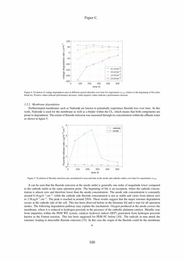
0 100 200 300 400 500
time /h
-250
-200
-150
-100
-50
0
50
100
volta
ge d
egra
datio
n ra
te /
V*h
-1
0.1 A*cm-2
0.5 A*cm-2
1.0 A*cm-2
2.0 A*cm-2
Figure 4: Evolution of voltage degradation rates at different current densities over time for experiment cyc10s relative to the beginning of life (afterbreak-in). Positive values indicate performance decrease, while negative values indicate a performance increase
3.2.2. Membrane degradationPerfluorinated membranes such as Nafion® are known to potentially experience fluoride loss over time. In this
work, Nafion® is used for the membrane as well as a binder within the CL, which means that both components areprone to degradation. The extent of fluoride emission was measured through its concentration within the effluent wateras shown in figure 5.
0 100 200 300 400 500
time /h
0
1
2
3
4
Flu
orid
e re
leas
e ra
te /
g*h-1
*cm
-2 cathodeanode
Figure 5: Evolution of fluoride emission rates normalized to area and time at the anode and cathode outlets over time for experiment cyc10s
It can be seen that the fluoride emission at the anode outlet is generally one order of magnitude lower comparedto the cathode outlet at the same operation point. The beginning of life is an exception, where the cathode concen-tration is almost zero and therefore lower than the anode concentration. The anode side concentration is constantlyaround 0.18 µg h−1 cm−2, while the cathode side fluoride concentration is not as stable and varies from almost zeroto 3.56 µg h−1 cm−2. The peak is reached at around 250 h. These results suggest that the major ionomer degradationoccurs at the cathode side of the cell. This has been observed before in the literature [6] and is true for all operationmodes. The following degradation pathway may explain the mechanism: Oxygen produced at the anode crosses themembrane, where it is reduced to hydrogen peroxide in the presence of the cathodic platinum catalyst. Metallic ionsfrom impurities within the PEM WE system, catalyze hydroxyl radical (HO•) generation from hydrogen peroxideknown as the Fenton reaction. This has been suggested for PEM FC before [10]. The radicals in turn attack theionomer, leading to detectable fluoride emission [15]. In this case the origin of the fluoride could be the membrane
6
Paper C.
100
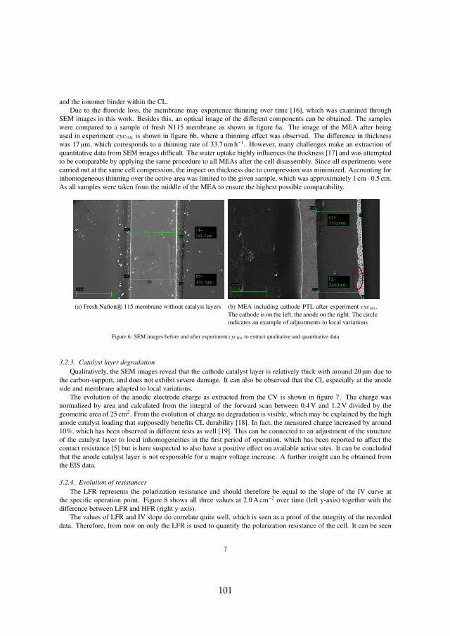
and the ionomer binder within the CL.Due to the fluoride loss, the membrane may experience thinning over time [16], which was examined through
SEM images in this work. Besides this, an optical image of the different components can be obtained. The sampleswere compared to a sample of fresh N115 membrane as shown in figure 6a. The image of the MEA after beingused in experiment cyc10s is shown in figure 6b, where a thinning effect was observed. The difference in thicknesswas 17 µm, which corresponds to a thinning rate of 33.7 nm h−1. However, many challenges make an extraction ofquantitative data from SEM images difficult. The water uptake highly influences the thickness [17] and was attemptedto be comparable by applying the same procedure to all MEAs after the cell disassembly. Since all experiments werecarried out at the same cell compression, the impact on thickness due to compression was minimized. Accounting forinhomogeneous thinning over the active area was limited to the given sample, which was approximately 1 cm · 0.5 cm.As all samples were taken from the middle of the MEA to ensure the highest possible comparability.
(a) Fresh Nafion® 115 membrane without catalyst layers (b) MEA including cathode PTL after experiment cyc10s.The cathode is on the left, the anode on the right. The circleindicates an example of adjustments to local variations
Figure 6: SEM images before and after experiment cyc10s to extract qualitative and quantitative data
3.2.3. Catalyst layer degradationQualitatively, the SEM images reveal that the cathode catalyst layer is relatively thick with around 20 µm due to
the carbon-support, and does not exhibit severe damage. It can also be observed that the CL especially at the anodeside and membrane adapted to local variations.
The evolution of the anodic electrode charge as extracted from the CV is shown in figure 7. The charge wasnormalized by area and calculated from the integral of the forward scan between 0.4 V and 1.2 V divided by thegeometric area of 25 cm2. From the evolution of charge no degradation is visible, which may be explained by the highanode catalyst loading that supposedly benefits CL durability [18]. In fact, the measured charge increased by around10%, which has been observed in different tests as well [19]. This can be connected to an adjustment of the structureof the catalyst layer to local inhomogeneities in the first period of operation, which has been reported to affect thecontact resistance [5] but is here suspected to also have a positive effect on available active sites. It can be concludedthat the anode catalyst layer is not responsible for a major voltage increase. A further insight can be obtained fromthe EIS data.
3.2.4. Evolution of resistancesThe LFR represents the polarization resistance and should therefore be equal to the slope of the IV curve at
the specific operation point. Figure 8 shows all three values at 2.0 A cm−2 over time (left y-axis) together with thedifference between LFR and HFR (right y-axis).
The values of LFR and IV slope do correlate quite well, which is seen as a proof of the integrity of the recordeddata. Therefore, from now on only the LFR is used to quantify the polarization resistance of the cell. It can be seen
7
101
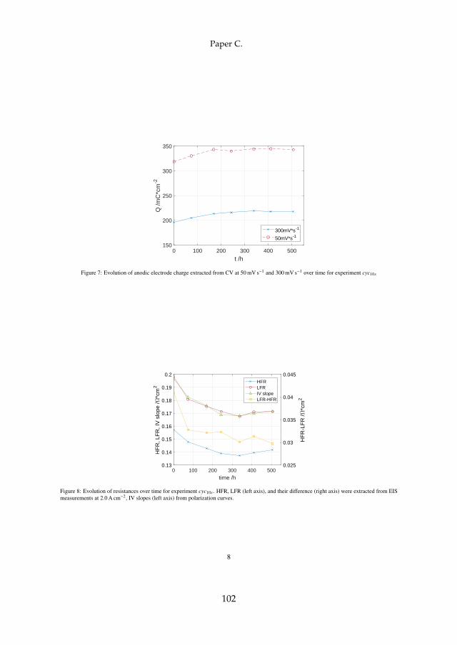
0 100 200 300 400 500
t /h
150
200
250
300
350
Q /m
C*c
m-2
300mV*s-1
50mV*s-1
Figure 7: Evolution of anodic electrode charge extracted from CV at 50 mV s−1 and 300 mV s−1 over time for experiment cyc10s
0 100 200 300 400 500
time /h
0.13
0.14
0.15
0.16
0.17
0.18
0.19
0.2
HF
R, L
FR
, IV
slo
pe /
*cm
2
0.025
0.03
0.035
0.04
0.045
HF
R-L
FR
/*c
m2
HFRLFRIV slopeLFR-HFR
Figure 8: Evolution of resistances over time for experiment cyc10s. HFR, LFR (left axis), and their difference (right axis) were extracted from EISmeasurements at 2.0 A cm−2, IV slopes (left axis) from polarization curves.
8
Paper C.
102
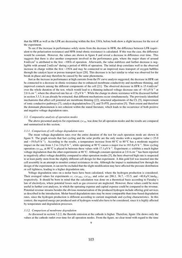
that the HFR as well as the LFR are decreasing within the first 338 h, before both show a slight increase for the rest ofthe experiment.
To see if the increase in performance solely stems from the decrease in HFR, the difference between LFR (equiv-alent to the polarization resistance) and HFR (total ohmic resistance) is calculated. If this was the case, the differencewould be constant. However, the values are shown in figure 8 and reveal a decrease in difference over time. Thissuggests that there is also another component involved in the performance gain, where the major share of around8 mΩ cm2 is attributed to the first ∼100 h of operation. Afterwards, the value stabilizes and further decrease is neg-ligible with around 2 mΩ cm2 during a period of 400 h of operation. The initial drop correlates well to the observedincrease in charge within the first ∼150 h and may be connected to an improved mass transport of oxygen bubblesthrough the catalyst layer or porous transport layer [20]. This decrease is in fact similar to what was observed for thebreak-in phase and may therefore be caused by the same phenomena.
Just as the increase in performance at high currents from the IV curve analysis suggested, the decrease in HFR canbe connected to a decrease in ohmic resistance due to enhanced membrane conductivity and membrane thinning, andimproved contacts among the different components of the cell [21]. The observed decrease in HFR is 15.4 mΩ cm2
over the whole duration of the test, which would lead to a thinning-induced voltage decrease rate of −61 µV h−1 at2.0 A cm−2, where the observed rate lies at −25 µV h−1. While the change in ohmic resistance will be discussed furtherin section 3.3.3, it can already be extracted, that different mechanisms occur simultaneously. The previously identifiedmechanisms that affect cell potential are membrane thinning [22], structural adjustments of the CL [5], improvementof ionic conductive pathways [7], catalyst degradation/loss [7], and Ti-PTL passivation [5]. Their extent and thereforethe dominant phenomenon is not coherent within the stated literature, which leads to the occurrence of both positiveand negative voltage degradation rates.
3.3. Comparative analysis of operation modesThe above presented analysis for experiment cyc10s was done for all operation modes and the results are compared
and summarized in this section.
3.3.1. Comparison of cell voltage degradation ratesThe mean voltage degradation rates over the entire duration of the test for each operation mode are shown in
figure 9. The graph reveals that fast cycling and the solar profile are the only modes with a negative value (−25.0and −19.0 µV h−1). According to the results, a temperature increase from 60 C to 80 C has a moderate negativeimpact on the rate from 1.2 to 3.0 µV h−1, while operating at 90 C causes a major rise to 183.8 µV h−1. Slow cyclingoperation cyc100s at 80 C is placed in between these values with 17.1 µV h−1. Experiment cc exhibits a much highervoltage degradation than the other experiments at 80 C. Although constant operation at 2.0 A cm−2 has been reportedto negatively affect voltage durability compared to other operation modes [5], the here observed high rate is suspectedto at least partly stem from the slightly different cell design for that experiment. A thin gold foil was inserted into thecell assembly in an attempt to monitor contact resistances in-situ. Although the impact is maintained low through thedesign of the experiment, it can not be excluded that the slight modification may have affected the pressure distributionor cell tightness, leading to a higher degradation rate.
Voltage degradation rates on a molar basis have been calculated, where the hydrogen production is considered.Their averaged values for experiments cc, cyc100s, cyc10s, and solar are 286.1, 36.7, −53.5, and −40.8 µV/molH2 ,respectively. It should be born in mind that the calculation was done on a theoretical basis according to Faraday’slaw of electrolysis, where potential losses such as gas crossover are neglected. However, these values could be moreuseful in further cost analyses, in which the operating expense and capital expense could be compared to the revenue.Potential revenue streams besides the obvious monetarization of the produced hydrogen include offering grid servicesas described in the introduction. Molar-based degradation rates may be more comparable than time-based degradationrates, since the hydrogen production is different according to current magnitude and cycling characteristics. In thiscontext, the required energy per produced unit of hydrogen would also have to be considered, since it is highly affectedby temperature and degradation processes.
3.3.2. Comparison of membrane degradationAs discussed in section 3.2.2, the fluoride emission at the cathode is higher. Therefore, figure 10a shows only the
values at the cathode outlet over time for all operation modes. From the figure, no clear trend with regard to the time
9
103
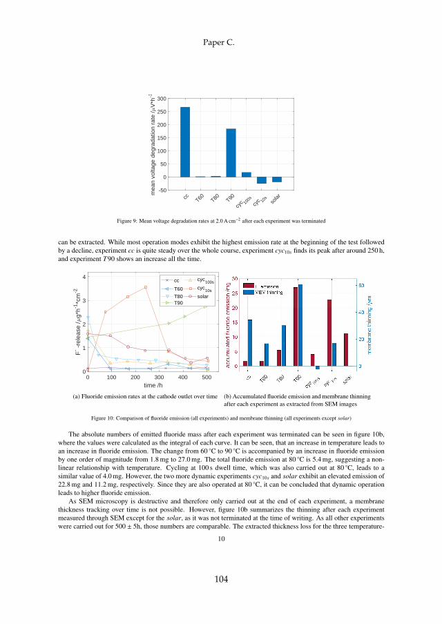
cc T60 T80 T90
cyc 10
0s
cyc 10
sso
lar-50
0
50
100
150
200
250
300
mea
n vo
ltage
deg
rada
tion
rate
/V
*h-1
Figure 9: Mean voltage degradation rates at 2.0 A cm−2 after each experiment was terminated
can be extracted. While most operation modes exhibit the highest emission rate at the beginning of the test followedby a decline, experiment cc is quite steady over the whole course, experiment cyc10s finds its peak after around 250 h,and experiment T90 shows an increase all the time.
0 100 200 300 400 500
time /h
0
1
2
3
4
F- -
rele
ase
/g*
h-1*c
m-2
cc
T60
T80T90
cyc100s
cyc10s
solar
(a) Fluoride emission rates at the cathode outlet over time (b) Accumulated fluoride emission and membrane thinningafter each experiment as extracted from SEM images
Figure 10: Comparison of fluoride emission (all experiments) and membrane thinning (all experiments except solar)
The absolute numbers of emitted fluoride mass after each experiment was terminated can be seen in figure 10b,where the values were calculated as the integral of each curve. It can be seen, that an increase in temperature leads toan increase in fluoride emission. The change from 60 C to 90 C is accompanied by an increase in fluoride emissionby one order of magnitude from 1.8 mg to 27.0 mg. The total fluoride emission at 80 C is 5.4 mg, suggesting a non-linear relationship with temperature. Cycling at 100 s dwell time, which was also carried out at 80 C, leads to asimilar value of 4.0 mg. However, the two more dynamic experiments cyc10s and solar exhibit an elevated emission of22.8 mg and 11.2 mg, respectively. Since they are also operated at 80 C, it can be concluded that dynamic operationleads to higher fluoride emission.
As SEM microscopy is destructive and therefore only carried out at the end of each experiment, a membranethickness tracking over time is not possible. However, figure 10b summarizes the thinning after each experimentmeasured through SEM except for the solar, as it was not terminated at the time of writing. As all other experimentswere carried out for 500 ± 5h, those numbers are comparable. The extracted thickness loss for the three temperature-
10
Paper C.
104
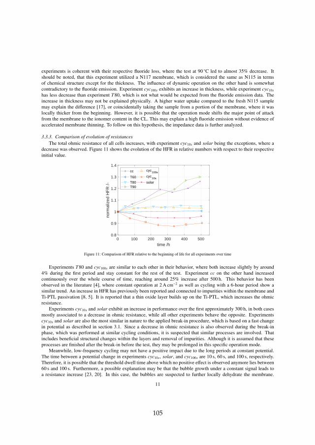
experiments is coherent with their respective fluoride loss, where the test at 90 C led to almost 35% decrease. Itshould be noted, that this experiment utilized a N117 membrane, which is considered the same as N115 in termsof chemical structure except for the thickness. The influence of dynamic operation on the other hand is somewhatcontradictory to the fluoride emission. Experiment cyc100s exhibits an increase in thickness, while experiment cyc10s
has less decrease than experiment T80, which is not what would be expected from the fluoride emission data. Theincrease in thickness may not be explained physically. A higher water uptake compared to the fresh N115 samplemay explain the difference [17], or coincidentally taking the sample from a portion of the membrane, where it waslocally thicker from the beginning. However, it is possible that the operation mode shifts the major point of attackfrom the membrane to the ionomer content in the CL. This may explain a high fluoride emission without evidence ofaccelerated membrane thinning. To follow on this hypothesis, the impedance data is further analyzed.
3.3.3. Comparison of evolution of resistancesThe total ohmic resistance of all cells increases, with experiment cyc10s and solar being the exceptions, where a
decrease was observed. Figure 11 shows the evolution of the HFR in relative numbers with respect to their respectiveinitial value.
0 100 200 300 400 500
time /h
0.8
0.9
1
1.1
1.2
1.3
1.4
norm
aliz
ed H
FR
/-
cc
T60
T80T90
cyc100s
cyc10s
solar
Figure 11: Comparison of HFR relative to the beginning of life for all experiments over time
Experiments T80 and cyc100s are similar to each other in their behavior, where both increase slightly by around4% during the first period and stay constant for the rest of the test. Experiment cc on the other hand increasedcontinuously over the whole course of time, reaching around 25% increase after 500 h. This behavior has beenobserved in the literature [4], where constant operation at 2 A cm−2 as well as cycling with a 6-hour period show asimilar trend. An increase in HFR has previously been reported and connected to impurities within the membrane andTi-PTL passivation [8, 5]. It is reported that a thin oxide layer builds up on the Ti-PTL, which increases the ohmicresistance.
Experiments cyc10s and solar exhibit an increase in performance over the first approximately 300 h, in both casesmostly associated to a decrease in ohmic resistance, while all other experiments behave the opposite. Experimentscyc10s and solar are also the most similar in nature to the applied break-in procedure, which is based on a fast changein potential as described in section 3.1. Since a decrease in ohmic resistance is also observed during the break-inphase, which was performed at similar cycling conditions, it is suspected that similar processes are involved. Thatincludes beneficial structural changes within the layers and removal of impurities. Although it is assumed that theseprocesses are finished after the break-in before the test, they may be prolonged in this specific operation mode.
Meanwhile, low-frequency cycling may not have a positive impact due to the long periods at constant potential.The time between a potential change in experiments cyc10s, solar, and cyc100s are 10 s, 60 s, and 100 s, respectively.Therefore, it is possible that the threshold dwell time above which no positive effect is observed anymore lies between60 s and 100 s. Furthermore, a possible explanation may be that the bubble growth under a constant signal leads toa resistance increase [23, 20]. In this case, the bubbles are suspected to further locally dehydrate the membrane.
11
105
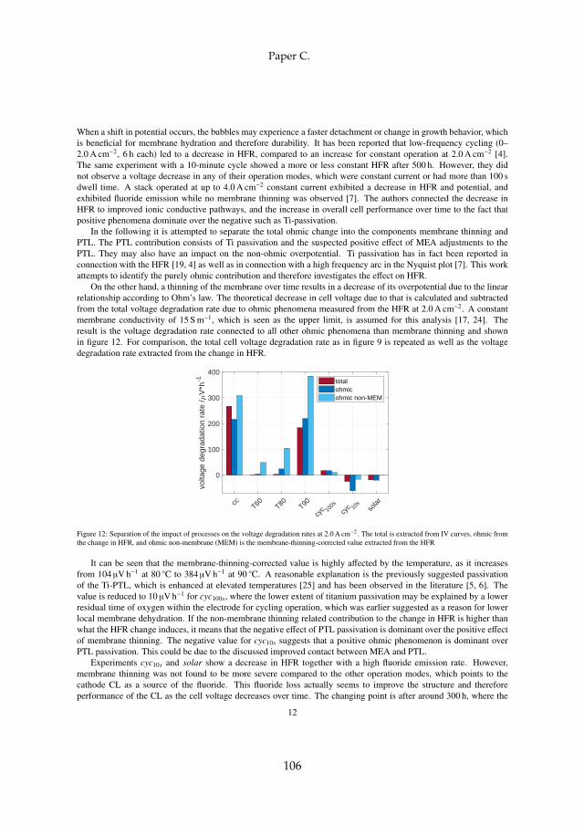
When a shift in potential occurs, the bubbles may experience a faster detachment or change in growth behavior, whichis beneficial for membrane hydration and therefore durability. It has been reported that low-frequency cycling (0–2.0 A cm−2, 6 h each) led to a decrease in HFR, compared to an increase for constant operation at 2.0 A cm−2 [4].The same experiment with a 10-minute cycle showed a more or less constant HFR after 500 h. However, they didnot observe a voltage decrease in any of their operation modes, which were constant current or had more than 100 sdwell time. A stack operated at up to 4.0 A cm−2 constant current exhibited a decrease in HFR and potential, andexhibited fluoride emission while no membrane thinning was observed [7]. The authors connected the decrease inHFR to improved ionic conductive pathways, and the increase in overall cell performance over time to the fact thatpositive phenomena dominate over the negative such as Ti-passivation.
In the following it is attempted to separate the total ohmic change into the components membrane thinning andPTL. The PTL contribution consists of Ti passivation and the suspected positive effect of MEA adjustments to thePTL. They may also have an impact on the non-ohmic overpotential. Ti passivation has in fact been reported inconnection with the HFR [19, 4] as well as in connection with a high frequency arc in the Nyquist plot [7]. This workattempts to identify the purely ohmic contribution and therefore investigates the effect on HFR.
On the other hand, a thinning of the membrane over time results in a decrease of its overpotential due to the linearrelationship according to Ohm’s law. The theoretical decrease in cell voltage due to that is calculated and subtractedfrom the total voltage degradation rate due to ohmic phenomena measured from the HFR at 2.0 A cm−2. A constantmembrane conductivity of 15 S m−1, which is seen as the upper limit, is assumed for this analysis [17, 24]. Theresult is the voltage degradation rate connected to all other ohmic phenomena than membrane thinning and shownin figure 12. For comparison, the total cell voltage degradation rate as in figure 9 is repeated as well as the voltagedegradation rate extracted from the change in HFR.
cc T60 T80 T90
cyc 10
0s
cyc 10
sso
lar
0
100
200
300
400
volta
ge d
egra
datio
n ra
te /
V*h
-1 totalohmicohmic non-MEM
Figure 12: Separation of the impact of processes on the voltage degradation rates at 2.0 A cm−2. The total is extracted from IV curves, ohmic fromthe change in HFR, and ohmic non-membrane (MEM) is the membrane-thinning-corrected value extracted from the HFR
It can be seen that the membrane-thinning-corrected value is highly affected by the temperature, as it increasesfrom 104 µV h−1 at 80 C to 384 µV h−1 at 90 C. A reasonable explanation is the previously suggested passivationof the Ti-PTL, which is enhanced at elevated temperatures [25] and has been observed in the literature [5, 6]. Thevalue is reduced to 10 µV h−1 for cyc100s, where the lower extent of titanium passivation may be explained by a lowerresidual time of oxygen within the electrode for cycling operation, which was earlier suggested as a reason for lowerlocal membrane dehydration. If the non-membrane thinning related contribution to the change in HFR is higher thanwhat the HFR change induces, it means that the negative effect of PTL passivation is dominant over the positive effectof membrane thinning. The negative value for cyc10s suggests that a positive ohmic phenomenon is dominant overPTL passivation. This could be due to the discussed improved contact between MEA and PTL.
Experiments cyc10s and solar show a decrease in HFR together with a high fluoride emission rate. However,membrane thinning was not found to be more severe compared to the other operation modes, which points to thecathode CL as a source of the fluoride. This fluoride loss actually seems to improve the structure and thereforeperformance of the CL as the cell voltage decreases over time. The changing point is after around 300 h, where the
12
Paper C.
106
HFR starts to slowly increase, may it be due to dominant PTL passivation or another process such as irreversiblecation contamination.
4. Conclusion
An analysis of degradation phenomena in PEM WE with a focus on the impact of operation modes was presented.Therefore, seven MEAs with the same specifications were run for 500 h each at constant, cycling, and dynamicoperation, where for constant operation the effect of temperature was also investigated. It was found that the CLonly played a minor role on degradation, while a change in total ohmic resistance dominated the voltage change.Subsequently, the respective shares of membrane and porous transport layer related phenomena were quantified.
It was found that Ti passivation is the major cause of voltage degradation at constant operation, dominating thevoltage decrease through membrane thinning. Operation at 90 C is favorable in terms of efficiency, but highly in-creases both Ti passivation and membrane thinning over time. Therefore, higher temperature can limit the lifetimeconsiderably due to increased gas crossover for a thinner membrane, while the passivation may revoke the gain inefficiency over time without an appropriate mitigation strategy.
On the other hand, fast cycling operation and simulating a direct coupling of the cell to a solar profile increased theoverall performance over the investigated time frame due to a decrease in ohmic resistance. It was furthermore foundthat fluoride emission is enhanced with fast potential switches, while no significant impact on membrane thicknesswas observed. Therefore, the fluoride is suspected to originate from the cathode catalyst layer.
Acknowledgement
The authors would like to acknowledge the support by Innovation Fund Denmark through the e-STORE project,Grant 4106-00025B.
References
[1] A. S. Arico, S. Siracusano, N. Briguglio, V. Baglio, A. Di Blasi, V. Antonucci, Polymer electrolyte membrane water electrolysis: Status oftechnologies and potential applications in combination with renewable power sources, Journal of Applied Electrochemistry 43 (2) (2013)107–118. doi:10.1007/s10800-012-0490-5.
[2] B. Bensmann, R. Hanke-Rauschenbach, G. Muller-Syring, M. Henel, K. Sundmacher, Optimal configuration and pressure levels of elec-trolyzer plants in context of power-to-gas applications, Applied Energy 167 (2016) 107124. doi:10.1016/j.apenergy.2016.01.038.URL http://dx.doi.org/10.1016/j.apenergy.2016.01.038
[3] G. A. Olah, A. Goeppert, G. S. Prakash, Beyond Oil and Gas: The Methanol Economy, Wiley-VCH, 2009.[4] C. Rakousky, U. Reimer, K. Wippermann, S. Kuhri, M. Carmo, W. Lueke, D. Stolten, Polymer electrolyte membrane water electrolysis: Re-
straining degradation in the presence of fluctuating power, Journal of Power Sources 342 (2017) 38–47. doi:10.1016/j.jpowsour.2016.11.118.URL http://dx.doi.org/10.1016/j.jpowsour.2016.11.118
[5] C. Rakousky, U. Reimer, K. Wippermann, M. Carmo, W. Lueke, D. Stolten, An analysis of degradation phenomena in polymer electrolytemembrane water electrolysis, Journal of Power Sources 326 (2016) 120–128. doi:http://dx.doi.org/10.1016/j.jpowsour.2016.06.082.
[6] F. Fouda-Onana, M. Chandesris, V. Medeau, S. Chelghoum, D. Thoby, N. Guillet, Investigation on the degradation of MEAs for PEM waterelectrolysers part I: Effects of testing conditions on MEA performances and membrane properties, International Journal of Hydrogen Energy41 (2016) 16627–16636. doi:10.1016/j.ijhydene.2016.07.125.
[7] P. Lettenmeier, R. Wang, R. Abouatallah, S. Helmly, T. Morawietz, R. Hiesgen, S. Kolb, F. Burggraf, J. Kallo, A. S. Gago, K. A. Friedrich,Durable Membrane Electrode Assemblies for Proton Exchange Membrane Electrolyzer Systems Operating at High Current Densities, Elec-trochimica Acta 210 (2016) 502–511. doi:10.1016/j.electacta.2016.04.164.URL http://dx.doi.org/10.1016/j.electacta.2016.04.164
[8] S. Sun, Z. Shao, H. Yu, G. Li, B. Yi, Investigations on degradation of the long-term proton exchange membrane water electrolysis stack,Journal of Power Sources 267 (2014) 515–520. doi:10.1016/j.jpowsour.2014.05.117.URL http://dx.doi.org/10.1016/j.jpowsour.2014.05.117
[9] M. Inaba, T. Kinumoto, M. Kiriake, R. Umebayashi, A. Tasaka, Z. Ogumi, Gas crossover and membrane degradation in polymer electrolytefuel cells, Electrochimica Acta 51 (26) (2006) 5746–5753. doi:10.1016/j.electacta.2006.03.008.
[10] A. B. LaConti, H. Liu, C. Mittelsteadt, R. C. M. Giner, POLYMER ELECTROLYTE MEMBRANE DEGRADATION MECHANISMS INFUEL CELLS FINDINGS OVER THE PAST 30 YEARS AND COMPARISON WITH ELECTROLYZERS, ECS Transactions 1 (8) (2006)199–219.
[11] FCH-JU, ANNUAL WORK PLAN and BUDGET, Tech. rep., FCH-JU (2017).[12] F. Hasche, Activity , stability , and degradation mechanisms of platinum and platinum alloy nanoparticle PEM fuel cell electrocatalysts, Ph.D.
thesis, TU Berlin (2012).
13
107
[13] M. Langemann, D. L. Fritz, M. Muller, D. Stolten, Validation and characterization of suitable materials for bipolar plates in PEM waterelectrolysis, International Journal of Hydrogen Energy 40 (35) (2015) 11385–11391. doi:10.1016/j.ijhydene.2015.04.155.
[14] V. B. Silva, A. Rouboa, Hydrogen-fed PEMFC: Overvoltage analysis during an activation procedure, Journal of Electroanalytical Chemistry671 (2012) 58–66. doi:10.1016/j.jelechem.2012.02.013.URL http://dx.doi.org/10.1016/j.jelechem.2012.02.013
[15] M. Chandesris, V. Medeau, N. Guillet, S. Chelghoum, D. Thoby, F. Fouda-Onana, Membrane degradation in PEM water electrolyzer: Nu-merical modeling and experimental evidence of the influence of temperature and current density, International Journal of Hydrogen Energy40 (3) (2015) 1353–1366. doi:10.1016/j.ijhydene.2014.11.111.
[16] F. N. F. Buchi, M. Inaba, T. J. T. T. J. Schmidt, Polymer Electrolyte Fuel Cell Durability, Springer, 2009.[17] H. Ito, T. Maeda, A. Nakano, H. Takenaka, Properties of Nafion membranes under PEM water electrolysis conditions, International Journal
of Hydrogen Energy 36 (17) (2011) 10527–10540. doi:10.1016/j.ijhydene.2011.05.127.URL http://dx.doi.org/10.1016/j.ijhydene.2011.05.127
[18] S. Cherevko, Stability and dissolution of electrocatalysts : Building the bridge between model and real world systems, Current Opinion inElectrochemistry (2018) 1–8doi:10.1016/j.coelec.2018.03.034.URL https://doi.org/10.1016/j.coelec.2018.03.034
[19] S. Siracusano, N. Hodnik, P. Jovanovic, F. Ruiz-Zepeda, M. Sala, V. Baglio, A. S. Arico, New insights into the stability of a high performancenanostructured catalyst for sustainable water electrolysis, Nano Energy 40 (September) (2017) 618–632. doi:10.1016/j.nanoen.2017.09.014.
[20] C. Lee, R. Banerjee, F. Arbabi, J. Hinebaugh, A. Bazylak, Porous Transport Layer Related Mass Transport Losses in Polymer ElectrolyteMembrane Electrolysis - A Review, Proceedings of the 14th International Conference on Nanochannels, Microchannels, and Minichannels.
[21] S. M. R. Niya, R. K. Phillips, M. Hoorfar, Process modeling of the impedance characteristics of proton exchange membrane fuel cells,Electrochimica Acta 191 (May) (2016) 1–117. doi:10.1016/j.electacta.2016.01.128.URL http://dx.doi.org/10.1016/j.electacta.2016.01.128
[22] S. Siracusano, N. Van Dijk, R. Backhouse, L. Merlo, V. Baglio, A. Arico, Degradation issues of PEM electrolysis MEAs, Renewable Energy123 (2018) 52–57. doi:10.1016/j.renene.2018.02.024.URL http://linkinghub.elsevier.com/retrieve/pii/S0960148118301678
[23] D. Kiuchi, H. Matsushima, Y. Fukunaka, K. Kuribayashi, Ohmic Resistance Measurement of Bubble Froth Layer in Water Electrolysis underMicrogravity, Journal of The Electrochemical Society 153 (8) (2006) E138. doi:10.1149/1.2207008.URL http://jes.ecsdl.org/cgi/doi/10.1149/1.2207008
[24] A. Kusoglu, B. L. Kienitz, A. Z. Weber, Understanding the Effects of Compression and Constraints on Water Uptake of Fuel-Cell Membranes,Journal ofThe Electrochemical Society 158 (12) (2011) 1504–1514. doi:10.1149/2.097112jes.
[25] G. Lu, S. L. Bernasek, J. Schwartz, Oxidation of a polycrystalline titanium surface by oxygen and water, Surface Science 458 (1) (2000)80–90. doi:10.1016/S0039-6028(00)00420-9.
14
Paper C.
108
Paper D
Impact of Iron and HydrogenPeroxide on MembraneDegradation for PEM WaterElectrolysis: Computationaland ExperimentalInvestigation on FluorideEmission
Steffen Henrik Frensch, Guillaume Serre, FrédéricFouda-Onana, Henriette Casper Jensen, Morten Lykkegaard
Christensen, Samuel Simon Araya, Søren Knudsen Kær
The paper has been submitted to theJournal of Power Sources.
109

submitted to an Elsevier Ltd. journal
Impact of Iron and Hydrogen Peroxide onMembraneDegradation for Polymer Electrolyte Membrane
Water Electrolysis: Computational and ExperimentalInvestigation on Fluoride Emission
Steffen Henrik Frenscha,∗, Guillaume Serreb, Frédéric Fouda-Onanab,Henriette Casper Jensenc, Morten Lykkegaard Christensenc, Samuel Simon
Arayaa, Søren Knudsen Kæra
aAalborg University, Department of Energy Technology, Pontoppidanstræde 111, 9220Aalborg Øst, Denmark
bCEA, LITEN, DEHT, F-38054, Grenoble, FrancecAalborg University, Department of Chemistry and Bioscience, Fredrik Bajers Vej 7, 9220
Aalborg Øst, Denmark
Abstract
Polymer electrolytemembrane (PEM)degradation in electrolysismode is sim-ulated through a Fentonmodel that includes all major involved electrochem-ical reactions. Supportive experimental investigations on the effect of hydro-gen peroxide and iron impurities are carried out in an ex-situ set-up, wherethe results are utilized to fit model parameters. The experiments reveal a highdependence of fluoride emission on iron concentration, which catalyzes thereaction, and identifies hydrogen peroxide as a necessary precursor for de-structive hydroxyl radical formation. Simulations of in-situ operation reveal
∗Corresponding author, (+45) 50 25 10 31Email addresses: [email protected] (Steffen Henrik Frensch), [email protected]
(Guillaume Serre), [email protected] (Frédéric Fouda-Onana),[email protected] (Henriette Casper Jensen), [email protected] (Morten LykkegaardChristensen), [email protected] (Samuel Simon Araya), [email protected] (Søren Knudsen Kær)
Preprint submitted to Journal of Power Sources November 8, 2018
111
that elevated current is favorable in terms of lower fluoride emission, as theradicals are depleted by side reactions. Temperatures above 80 C significantlyaccelerate membrane thinning, where the step from 80 C to 90 C more thandoubles thinning after 500 h.Keywords: PEMwater electrolysis aging, Membrane degradation modelling,Fenton reaction model, Hydrogen peroxide, Fluoride emission rate
Nomenclature
1. Introduction
Membrane degradation for polymer electrolytemembrane water electrol-ysis (PEM WE) is crucial, since it does not only have an impact on cell per-formance, but also directly affects operation safety. Membrane thinning asa result of degradation increases gas crossover, possibly leading to explosivemixtures [1, 2]. The membrane is therefore considered as one of the lifetimelimiting components of a PEMWE system [2]. Membrane degradation in PEMWE is not yet fully understood, but the here described mechanism has beensuggested in the literature [2]. Besides protons (H+) andwater (H2O), also oxy-gen (O2) is transported through themembrane from the anode to the cathodeside. In the presence of a platinum catalyst, as it is the case in a state of theart PEM WE cathode (C Lc), oxygen and protons react to form hydrogen per-oxide (H2O2) according to equation I [3]:
O2 +2H++2e− −−−→ H2O2 (I)
In turn, the produced H2O2 forms highly reactive hydroxyl radicals (HO•).This reaction is strongly catalyzed by ferrous iron ions (Fe2+) and under that
2
Paper D.
112
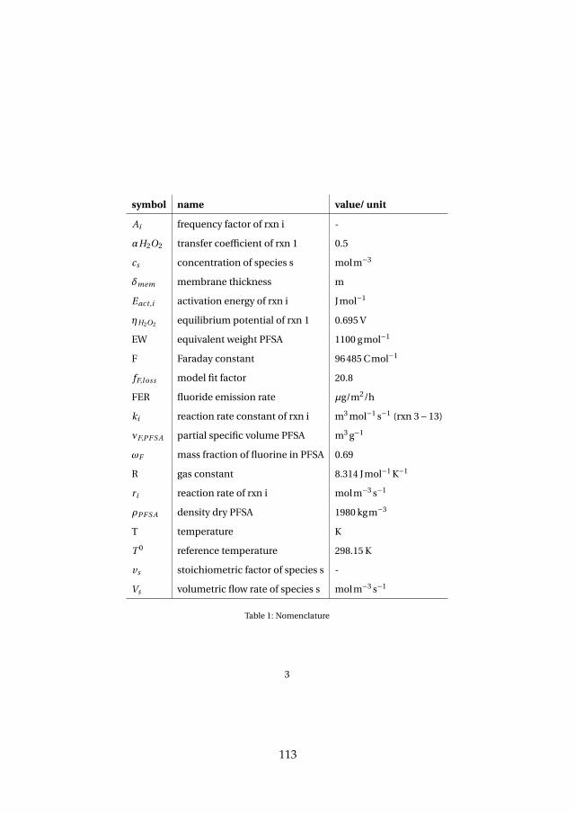
symbol name value/ unit
Ai frequency factor of rxn i -αH2O2 transfer coefficient of rxn 1 0.5cs concentration of species s molm−3
δmem membrane thickness m
Eact ,i activation energy of rxn i Jmol−1
ηH2O2 equilibrium potential of rxn 1 0.695 V
EW equivalent weight PFSA 1100 gmol−1
F Faraday constant 96485 Cmol−1
fF,loss model fit factor 20.8
FER fluoride emission rate µg/m2/h
ki reaction rate constant of rxn i m3 mol−1 s−1 (rxn 3 – 13)νF,PF S A partial specific volume PFSA m3 g−1
ωF mass fraction of fluorine in PFSA 0.69R gas constant 8.314 Jmol−1 K−1
ri reaction rate of rxn i molm−3 s−1
ρPF S A density dry PFSA 1980 kgm−3
T temperature K
T 0 reference temperature 298.15 K
vs stoichiometric factor of species s -Vs volumetric flow rate of species s molm−3 s−1
Table 1: Nomenclature
3
113
condition well known as the Fenton reaction as seen in equation II:
H2O2 +Fe2+ −−−→ Fe3++HO•+HO− (II)
Theexactmechanismsof theFenton reactionarenot yet fullyunderstood [4],but assumed toplay a role in PEMWEdegradation. It is commonly agreed thatmetallic impurities such as iron ions accelerate membrane attack in the pres-ence of H2O2. These iron impurities may stem from the balance of plant [2],however, this claim has yet to be proven and further developed. The assump-tion is that all componentsmade of stainless steel such as the the cell housingand the piping system release iron ions over time [5]. The behavior of ironwithin the system is not well documented, i.e. the ions may cross the mem-brane, stay within it, or be flushed out at one of the outlets. An accumulationof ions would increase the concentration over time, which may affect the re-action kinetics. The radicals formed through the Fenton reaction may attackthe membrane structure, which leads to a release of fluoride in the case ofNafion®.
Although theoperating conditions and therefore the reactionenvironmentis different in PEM WE, the underlying mechanisms may be deduced fromPEM fuel cell (FC) research, since the state of the art membrane material isusually the same. A good PEM FC review can be found in the literature [6]that summarizes the proposal that hydrogen peroxide (H2O2) decompositionis highly involved in chemical degradation. This claim is challenged by an ex-perimental investigation, which finds H2O2 to be responsible for only a smallfraction of membrane degradation [7]. With or without involvement of H2O2,radicals may attack the ionomer binder within the catalyst layer, at the inter-
4
Paper D.
114
face between catalyst layer and membrane, or diffuse from the cathode elec-trode back into the membrane, where it can also attack the ionomer.
A modelling framework for chemical degradation based on radical attackas described above was proposed in [8], who resolved the membrane and as-sumed the above mentioned involvement of H2O2. Similarily, a comprehen-sive simulation with a focus on radical formation through H2O2 comparesperfluoroalkyl sulfonic acid (PFSA) membranes to poly(styrenesulfonic acid)(PSSA) membranes and includes an ex-situ Fenton reaction simulation [9].The authors find very different attack mechanisms for both membrane typesand reveal a higher FER for the ex-situ test by 2-3 orders of magnitude. Thepoints of attack and the evolution of their availability in PFSAmembraneswassimulated by [10], who found a more severe impact of iron ion concentrationcompared to H2O2 on radical formation. Finally, semi-empirical degradationdata was incorporated into a model to simulate membrane thinning in [11].
As for PEM WE, a model approach similar to the ones found for PEM FCis described in the literature [12]. The work is based on modelling and exper-imental data to simulate membrane attack accompanied by membrane thin-ning. However, the degradation behavior of both are not fully identical [13]and compared to PEM FC, studies dedicated to PEM WE remain scarce. Ex-perimentally, the effect of current density on fluoride emission rate (FER) wasinvestigated in [14], who found a peak between 0.2 and 0.4 Am−2. The authorsfurthermore reported that a majority of membrane degradation can be ob-served on the cathode side [14], which supports the presented degradationmechanism.
This work aims at developing the presented modelling approach further
5
115
for PEMWE applications and operation strategies. Furthermore, the simula-tions are supported by experimental data that investigates the effect of hydro-gen peroxide and iron ions on fluoride release.
2. Experimental Methodology
Eleven polypropylene flasks were filled with 100 mL ultra-pure water forthe ex-situ experiment. A specific initial concentration of Fe2+ and H2O2 ac-cording to table 2 was established based on a literature review of previoustests [15, 9, 7]. The iron concentration was set through iron (II) sulfate hep-tahydrate (FeSO4 ·7H2O,Merck KGaA) and the hydrogen peroxide concentra-tion through 33%-H2O2 solution (VWR Chemicals). 25 cm2 Nafion® 115 cutinto five pieces was immersed and each experiment lasted for 72 h at 80 C
inside an oven. The fluoride content was monitored frequently with an ionselective electrode (ISE, Hach Company ISE301F combined electrode).
3. Model Development
The degradation processes are assumed to be as described above and de-picted in figure 1.
The model approach is carried out in Matlab/Simulink® and consists ofa 0-dimensional membrane degradationmodel, which is implemented into asimple performance model. Membrane degradation is among the most cru-cial mechanisms for PEM WE and can be considered a lifetime-limiting fac-tor [2]. Therefore, capturing the membrane degradation over time throughchemical attack is simulated as described above. The Fenton model calcu-lates fluoride emission through concentration of species such as H2O2, and
6
Paper D.
116
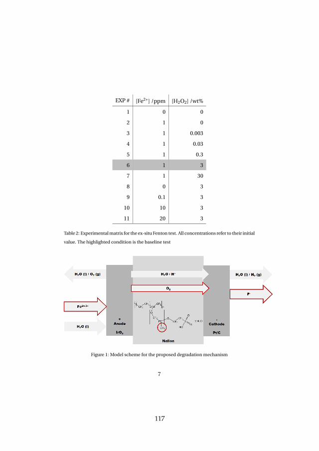
EXP # [Fe2+] /ppm [H2O2] /wt%
1 0 02 1 03 1 0.0034 1 0.035 1 0.36 1 37 1 308 0 39 0.1 310 10 311 20 3
Table 2: Experimentalmatrix for the ex-situ Fenton test. All concentrations refer to their initialvalue. The highlighted condition is the baseline test
Figure 1: Model scheme for the proposed degradation mechanism
7
117
the involved radicals. In its core, the description of the involved electrochem-ical reaction system is based on [12]. In this work, a set of 14 electrochemicalreactions was modelled as one reaction system. An overview over the consid-ered reactions is given in table 3.
The main assumptions are:
• all 14 reactions occur in the same space (C Lc)
• oxygen transported to the cathode is entirely and exclusively reduced tohydrogen peroxide (reaction 1)
• reactions 2-13 follow Arrhenius behavior
• the total fluoride emission (reaction 14) as a macroscopic reaction be-haves like an elementary reaction (i.e. also follows Arrhenius behavior)
3.1. Reaction System and Rate Constants
In a coarse-grained approach, the rate constants at 25 C and the activa-tion energies for reactions 2 to 13 (except for reactions 7, where data for onlyone temperature was found) were fitted to the Arrhenius equation as in equa-tion III:
k = A ·exp(−Eact
R ·T) (III)
where k is the rate constant, A the frequency factor in s−1 (also known as thepre-exponential factor), Eact the activation energy in Jmol−1, R the gas con-stant in Jmol−1 K−1, and T the temperature in K. The rate constant for eachreactionwas then implementedas a functionof temperature. Reaction1 is im-plemented as described in section 3.2, while reaction 14 is further addressed
8
Paper D.
118
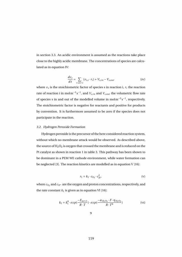
in section 3.3. An acidic environment is assumed as the reactions take placeclose to the highly acidicmembrane. The concentrations of species are calcu-lated as in equation IV:
dcs
d t=
∑
r xn=i(vs,i · ri )+Vs,i n −Vs,out (IV)
where vs is the stoichiometric factor of species s in reaction i, ri the reactionrate of reaction i in molm−3 s−1, and Vs,i n and Vs,out the volumetric flow rateof species s in and out of the modelled volume in molm−3 s−1, respectively.The stoichiometric factor is negative for reactants and positive for productsby convention. It is furthermore assumed to be zero if the species does notparticipate in the reaction.
3.2. Hydrogen Peroxide Formation
Hydrogenperoxide is theprecursorof thehere considered reaction system,without which no membrane attack would be observed. As described above,the source ofH2O2 is oxygen that crossed themembrane and is reducedon thePt catalyst as shown in reaction 1 in table 3. This pathway has been shown tobe dominant in a PEM WE cathode environment, while water formation canbe neglected [3]. The reaction kinetics are modelled as in equation V [16]:
r1 = k1 · cO2 · c2H+ (V)
where cO2 and cH+ are theoxygenandprotonconcentrations, respectively, andthe rate constant k1 is given as in equation VI [16]:
k1 = k01 ·exp(
−Eact ,1
R ·T) ·exp(
−αH2O2 ·F ·ηH2O2
R ·T 0) (VI)
9
119
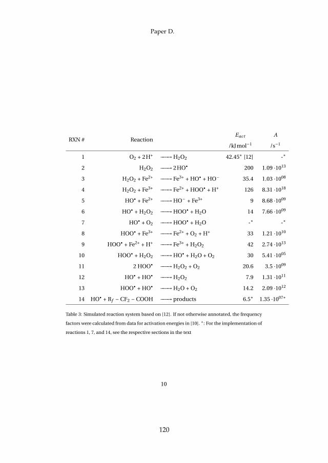
RXN # ReactionEact
/kJmol−1
A
/s−1
1 O2 + 2H+ −−−→H2O2 42.45∗ [12] -∗
2 H2O2 −−−→ 2HO• 200 1.09 ·1013
3 H2O2 + Fe2+ −−−→ Fe3+ + HO• + HO– 35.4 1.03 ·1008
4 H2O2 + Fe3+ −−−→ Fe2+ + HOO• + H+ 126 8.31 ·1018
5 HO• + Fe2+ −−−→HO– + Fe3+ 9 8.68 ·1009
6 HO• + H2O2 −−−→HOO• + H2O 14 7.66 ·1009
7 HO• + O2 −−−→HOO• + H2O -∗ -∗
8 HOO• + Fe3+ −−−→ Fe2+ + O2 + H+ 33 1.21 ·1010
9 HOO• + Fe2+ + H+ −−−→ Fe3+ + H2O2 42 2.74 ·1013
10 HOO• + H2O2 −−−→HO• + H2O + O2 30 5.41 ·1005
11 2 HOO• −−−→H2O2 + O2 20.6 3.5 ·1009
12 HO• + HO• −−−→H2O2 7.9 1.31 ·1011
13 HOO• + HO• −−−→H2O + O2 14.2 2.09 ·1012
14 HO• + Rf – CF2 – COOH −−−→products 6.5∗ 1.35 ·1007∗
Table 3: Simulated reaction system based on [12]. If not otherwise annotated, the frequencyfactors were calculated from data for activation energies in [10]. ∗: For the implementation ofreactions 1, 7, and 14, see the respective sections in the text
10
Paper D.
120
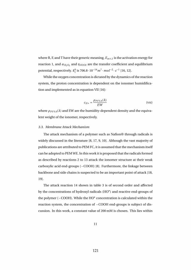
where R, F, andThave their genericmeaning, Eact ,1 is the activation energy forreaction 1, and αH2O2 and ηH2O2 are the transfer coefficient and equilibriumpotential, respectively. k0
1 is 706.8 ·10−14m7 ·mol−2 · s−1 [16, 12].While the oxygen concentration is dictated by the dynamics of the reaction
system, the proton concentration is dependent on the ionomer humidifica-tion and implemented as in equation VII [16]:
cH+ = ρPF S A(λ)
EW(VII)
where ρPF S A(λ) and EW are the humidity-dependent density and the equiva-lent weight of the ionomer, respectively.
3.3. Membrane Attack Mechanism
The attack mechanism of a polymer such as Nafion® through radicals iswidely discussed in the literature [8, 17, 9, 10]. Although the vast majority ofpublications are attributed to PEMFC, it is assumed that themechanism itselfcanbe adopted to PEMWE. In thiswork it is proposed that the radicals formedas described by reactions 2 to 13 attack the ionomer structure at their weakcarboxylic acid end-groups ( –COOH) [8]. Furthermore, the linkage betweenbackbone and side chains is suspected to be an important point of attack [18,19].
The attack reaction 14 shown in table 3 is of second order and affectedby the concentrations of hydroxyl radicals (HO•) and reactive end-groups ofthe polymer ( –COOH). While the HO• concentration is calculated within thereaction system, the concentration of –COOH end-groups is subject of dis-cussion. In this work, a constant value of 200 mM is chosen. This lies within
11
121
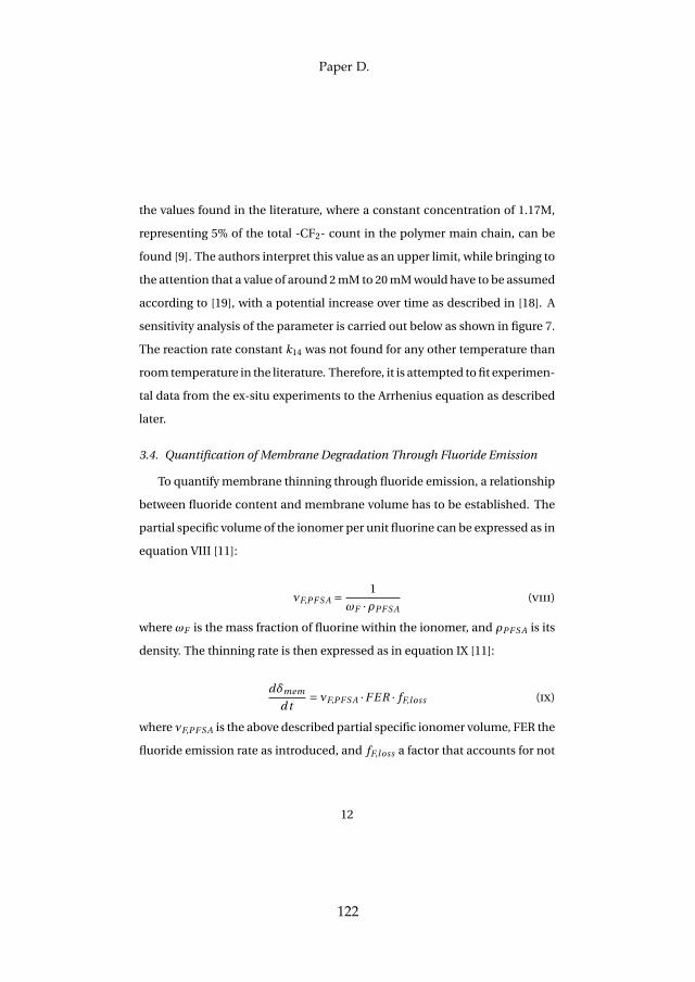
the values found in the literature, where a constant concentration of 1.17M,representing 5% of the total -CF2- count in the polymer main chain, can befound [9]. The authors interpret this value as an upper limit, while bringing tothe attention that a value of around 2 mM to 20 mMwould have to be assumedaccording to [19], with a potential increase over time as described in [18]. Asensitivity analysis of the parameter is carried out below as shown in figure 7.The reaction rate constant k14 was not found for any other temperature thanroomtemperature in the literature. Therefore, it is attempted tofit experimen-tal data from the ex-situ experiments to the Arrhenius equation as describedlater.
3.4. Quantification of Membrane Degradation Through Fluoride Emission
To quantify membrane thinning through fluoride emission, a relationshipbetween fluoride content and membrane volume has to be established. Thepartial specific volume of the ionomer per unit fluorine can be expressed as inequation VIII [11]:
νF,PF S A = 1
ωF ·ρPF S A(VIII)
where ωF is the mass fraction of fluorine within the ionomer, and ρPF S A is itsdensity. The thinning rate is then expressed as in equation IX [11]:
dδmem
d t= νF,PF S A ·F ER · fF,l oss (IX)
where νF,PF S A is the above described partial specific ionomer volume, FER thefluoride emission rate as introduced, and fF,loss a factor that accounts for not
12
Paper D.
122
captured fluoride ions and incompletely decomposed fluorine. It is imple-mented relative to each captured fluoride ion and therefore technically hasthe unit gg−1, which means it is dimensionless. The extent of total fluorineemission is not widely reported, but FC research indicates that it might bea considerable share [20]. Therefore, membrane thinning may be underesti-mated in this approach. On the other hand, all fluoride emission is accountedfor membrane thinning, while the ionomer binder in the catalyst layers mayalso contribute to the total fluoride emission. It is experimentally impracticalto differentiate between the origin of fluoride, which may lead to an overesti-mation of membrane thinning.
4. Results and Discussion
4.1. Ex-situ Fluoride Emission
The fluoride concentration for each experiment over time is shown in fig-ure 2. Experiments with varying initial H2O2 concentration are shown in solidlines and varying initial Fe2+ concentrations in dashed lines together with thebaseline and the pure water test in dash-dot lines.
As expected, the test with neither H2O2 nor Fe2+ initially (#1) only showsa negligible fluoride release, which might be a consequence of hygrothermalaging [21]. The experiment with no H2O2 and 1 ppm Fe2+ (#2) also exhibits al-most no fluoride emission, while the presence of 3wt% H2O2 but no Fe2+ (#8)lead to a considerable fluoride concentration especially towards the endof theexperiment of around 1 ppm. This observation supports the above presentedassumption that H2O2 is as a obligatory precursor for the whole reaction sys-tem, while Fe2+ acts as a catalyst.
13
123
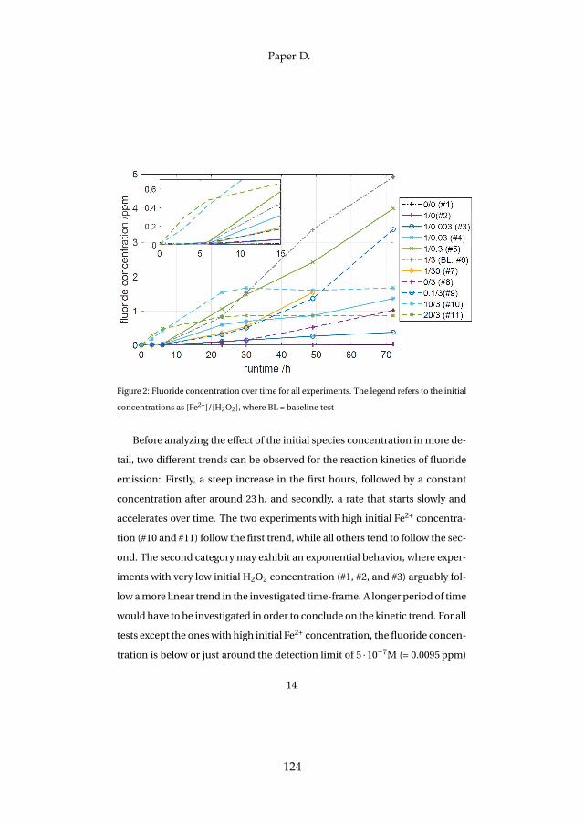
Figure 2: Fluoride concentration over time for all experiments. The legend refers to the initialconcentrations as [Fe2+]/[H2O2], where BL = baseline test
Before analyzing the effect of the initial species concentration inmore de-tail, two different trends can be observed for the reaction kinetics of fluorideemission: Firstly, a steep increase in the first hours, followed by a constantconcentration after around 23 h, and secondly, a rate that starts slowly andaccelerates over time. The two experiments with high initial Fe2+ concentra-tion (#10 and #11) follow the first trend, while all others tend to follow the sec-ond. The second category may exhibit an exponential behavior, where exper-iments with very low initial H2O2 concentration (#1, #2, and #3) arguably fol-low amore linear trend in the investigated time-frame. A longer period of timewould have to be investigated in order to conclude on the kinetic trend. For alltests except the oneswith high initial Fe2+ concentration, the fluoride concen-tration is below or just around the detection limit of 5 ·10−7M (= 0.0095 ppm)
14
Paper D.
124
within the first 3 to 6 hours of test as shown in the magnification in figure 2.Theflatteningof the curveswithhigh initial Fe2+ concentrationmaybedue
toH2O2 exhaustion. With Fe2+ as a strong catalyst, the neededH2O2 to run thereaction may be used up very fast and therefore represent the limiting factorin these experiments. Consequently, the final fluoride concentration after thetestwas terminatedmaybe significantly higher ifmoreH2O2was available, ei-ther as an initial concentration or as a steady influx. It can in fact be observed,that the higher initial Fe2+ concentration of 20 ppm leads to higher fluorideemission than 10 ppm as measured after 3 h as shown in the magnification infigure 2. Possibly due to the same limiting effect, 20 ppm Fe2+ (#11) producedless fluoride emission than 10 ppm Fe2+ (#10) at the sameH2O2 concentrationafter 6 hours. Therefore, a peak appears at 10 ppm after 23 h when plottingthe fluoride concentration over initial Fe2+ concentration as seen in figure 3a,which shifts to 1 ppm after 49 h.
When looking at the experimentwithout any initial Fe2+ (#8), an unexpect-edly high fluoride emission can be observed. Although Fe2+ only acts as a cat-alyst and is theoretically not necessary to produce HO• radicals as shown inreaction 2, simulations of experiment #8 reveal that a fluoride concentrationclose to zero is expected after 72 h, as can be seen in figure 4b. This discrep-ancy might be explained by the presence of other metal impurities such ascopper ions (Cu2+) in the solution, which catalyze the Fenton reaction but arenot implemented in the model [22, 23]. They may stem for example from themembrane manufacturing process or the feed water that may not be purifiedperfectly. Furthermore, it has been shown in the literature that Fe2+maybe re-placedbyother Fenton-likemetal catalysts toproduceHO• radicals, including
15
125
titanium [24, 25]. Reactions between other metal impurities and H2O2 can beimplemented similarly as done with Fe2+ in this work.
The impact of initial H2O2 concentration on fluoride emission at 1 ppm
initial Fe2+ concentration can be seen in figure 3b. As for iron, the figure in-cludesmeasurements after 23 h (blue) and 49 h (red). Besides the abovemen-tioned zero-emission at the absence of H2O2, a dependency is visible. Whilelow initialH2O2 concentration leads to lowfluorideemission, thepeak is reachedbetween 0.03 and 30wt%, depending on the considered time-frame. This sug-gests the existence of an optimal concentration to prevent excessive mem-brane degradation outside these boundaries. Simulations have confirmed thetheoretical existenceof suchanoptimumandwill bediscussed later. However,intuitively an increase in fluoride emission with H2O2 concentration wouldbe expected. A repetition of the set of experiments has to be carried out inorder to finally conclude on the existence of an optimum and to rule out ex-perimental errors. An ex-situ experiment was carried out in the literature tofind the dependence of the fluoride emission on temperature at 0.36 mM Fe2+
(≈ 20 ppm) and 9.68 M H2O2 (≈33wt%) [15]. They found a concentration ofroughly 0.38 ppm F– after 9.5 h at 80 C. The conditions are different fromany of the here investigated ones, but come closest to experiment #7 with30wt%H2O2 and 1 ppm Fe2+, where themeasured fluoride concentration was0.35 ppm after 23 h.
4.1.1. Implications on the Membrane Attack Reaction
Themodel described above is utilized in order to simulate ex-situ behaviorand adjusted by setting all in- and outflux to zero. Instead, the initial concen-trations of Fe2+ and H2O2 are set according to the test as in table 2. Further-
16
Paper D.
126
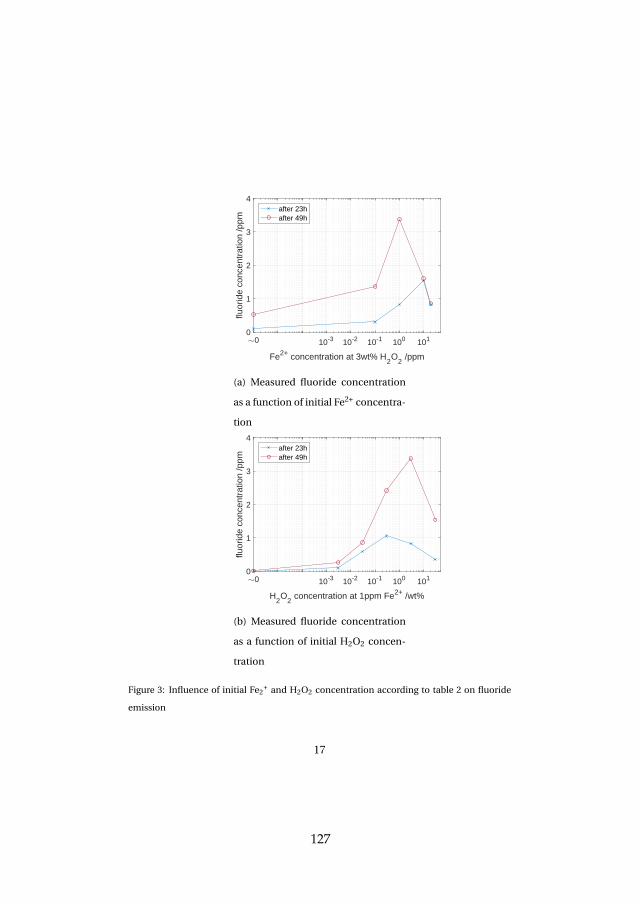
0 10-3 10-2 10-1 100 101
Fe2+ concentration at 3wt% H2O
2 /ppm
0
1
2
3
4
fluor
ide
conc
entr
atio
n /p
pm
after 23hafter 49h
(a) Measured fluoride concentration
as a function of initial Fe2+ concentra-
tion
0 10-3 10-2 10-1 100 101
H2O
2 concentration at 1ppm Fe2+ /wt%
0
1
2
3
4
fluor
ide
conc
entr
atio
n /p
pm
after 23hafter 49h
(b) Measured fluoride concentration
as a function of initial H2O2 concen-
tration
Figure 3: Influence of initial Fe2+ and H2O2 concentration according to table 2 on fluorideemission
17
127
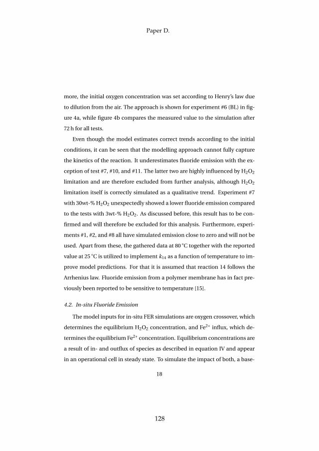
more, the initial oxygen concentration was set according to Henry’s law dueto dilution from the air. The approach is shown for experiment #6 (BL) in fig-ure 4a, while figure 4b compares the measured value to the simulation after72 h for all tests.
Even though the model estimates correct trends according to the initialconditions, it can be seen that the modelling approach cannot fully capturethe kinetics of the reaction. It underestimates fluoride emission with the ex-ception of test #7, #10, and #11. The latter two are highly influenced by H2O2
limitation and are therefore excluded from further analysis, although H2O2
limitation itself is correctly simulated as a qualitative trend. Experiment #7with 30wt-%H2O2 unexpectedly showed a lower fluoride emission comparedto the tests with 3wt-% H2O2. As discussed before, this result has to be con-firmed and will therefore be excluded for this analysis. Furthermore, experi-ments #1, #2, and #8 all have simulated emission close to zero and will not beused. Apart from these, the gathered data at 80 C together with the reportedvalue at 25 C is utilized to implement k14 as a function of temperature to im-prove model predictions. For that it is assumed that reaction 14 follows theArrhenius law. Fluoride emission from a polymer membrane has in fact pre-viously been reported to be sensitive to temperature [15].
4.2. In-situ Fluoride Emission
The model inputs for in-situ FER simulations are oxygen crossover, whichdetermines the equilibrium H2O2 concentration, and Fe2+ influx, which de-termines the equilibrium Fe2+ concentration. Equilibrium concentrations area result of in- and outflux of species as described in equation IV and appearin an operational cell in steady state. To simulate the impact of both, a base-
18
Paper D.
128
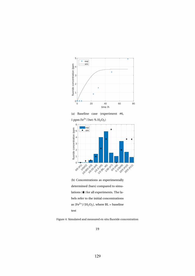
0 20 40 60 80
time /h
0
1
2
3
4
5
fluor
ide
conc
entr
atio
n /p
pm
expsim
(a) Baseline case (experiment #6,
1 ppm Fe2+/3wt-% H2O2)
0/0
(#1)
1/0(
#2)
1/0.
003
(#3)
1/0.
03 (#
4)
1/0.
3 (#
5)
1/3
(BL,
#6)
1/30
(#7)
0/3
(#8)
0.1/
3(#9
)
10/3
(#10
)
20/3
(#11
)0
1
2
3
4
5
6
fluor
ide
conc
entr
atio
n /p
pm
expsim
(b) Concentrations as experimentally
determined (bars) compared to simu-
lations () for all experiments. The la-
bels refer to the initial concentrations
as [Fe2+]/[H2O2], where BL = baseline
test
Figure 4: Simulated andmeasured ex-situ fluoride concentration
19
129
line for O2 crossover was set to 6 · 10−5molm−2 s−1, leading to around = 7.6 ·10−3M H2O2 equilibrium concentration. This is in fair agreement with the as-sumed constant background H2O2 concentration of = 5 · 10−4M in [9] whenconsidering that this number will change according to the operation condi-tion. The O2 permeation rate was found in the literature as experimentallydetermined at 2.0 Acm−2 and 70 C [26]. The baseline Fe2+ influx is set to 3.58 ·10−7molm−2 s−1 (= 1 ppm·s−1), leading to 2.6 ·10−5M (= 0.13 ppm) equilibriumconcentration. The Fe2+ influx was chosen as a starting point and is slightlylower than what was found in a previous simulation work [12]. Setting an in-and outflux rather than a constant background concentration assumes thatFe2+ has a source term outside the MEA, which might be any stainless steelcomponent in the cell assembly or balance of plant. Lastly, the baseline cur-rent was set to 2.0 Acm−2 and the temperature to 80 C.
The model results show that oxygen is needed to produce H2O2, but doesnot play a vital role in the reaction systemotherwise. H2O2 formationhoweveris crucial, as it serves as a precursor for all other reactions. This is supportedbythe ex-situ experiment, where the two tests without H2O2 (#1 and #2) lead toa fluoride emission close to zero. The driving force for the membrane attackas in reaction 14 is the HO• radical. Therefore, a lower concentration leadsto a lower simulated FER as it can be seen in figure 5. The cause for a lowerHO• concentration at higher current can be foundwithin reactions 3, 6, and 7,which are also shown in the figure. While reaction 3 is the dominant pathwayfor radical production, reactions 6 and 7 are its major sinks besides the attackreaction 14. It can be observed that the reaction rate of reaction 3 decreaseswith increasing current, whereas the rate for reaction 7 increases. Therefore,
20
Paper D.
130
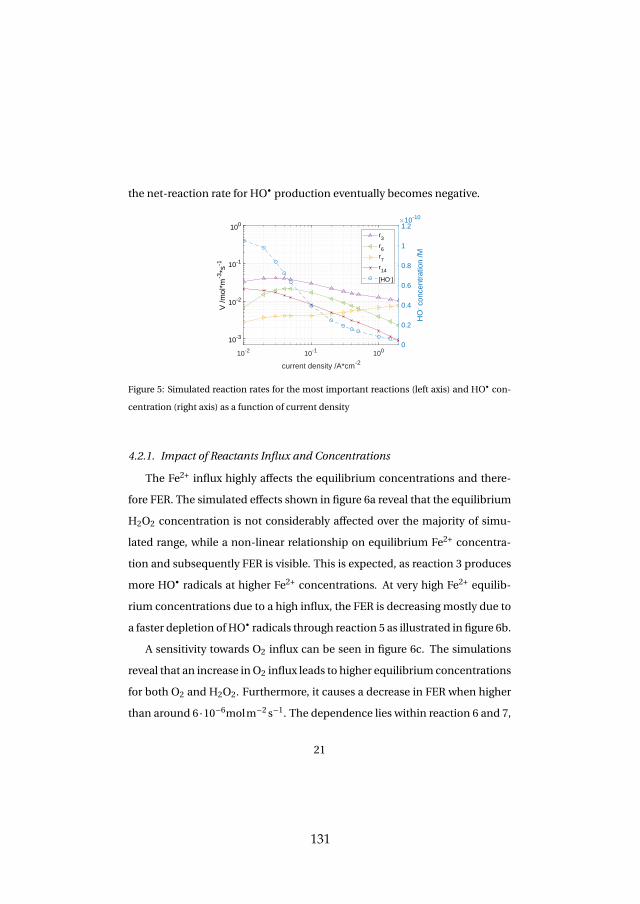
the net-reaction rate for HO• production eventually becomes negative.
10-2 10-1 100
current density /A*cm-2
10-3
10-2
10-1
100V
/mol
*m-3
*s-1
0
0.2
0.4
0.6
0.8
1
1.2
HO
. con
cent
ratio
n /M
10-10
r3
r6
r7
r14
[HO.]
Figure 5: Simulated reaction rates for the most important reactions (left axis) and HO• con-centration (right axis) as a function of current density
4.2.1. Impact of Reactants Influx and Concentrations
The Fe2+ influx highly affects the equilibrium concentrations and there-fore FER. The simulated effects shown in figure 6a reveal that the equilibriumH2O2 concentration is not considerably affected over the majority of simu-lated range, while a non-linear relationship on equilibrium Fe2+ concentra-tion and subsequently FER is visible. This is expected, as reaction 3 producesmore HO• radicals at higher Fe2+ concentrations. At very high Fe2+ equilib-rium concentrations due to a high influx, the FER is decreasing mostly due toa faster depletion of HO• radicals through reaction 5 as illustrated in figure 6b.
A sensitivity towards O2 influx can be seen in figure 6c. The simulationsreveal that an increase inO2 influx leads to higher equilibrium concentrationsfor both O2 and H2O2. Furthermore, it causes a decrease in FER when higherthan around 6 ·10−6molm−2 s−1. The dependence lies within reaction 6 and 7,
21
131
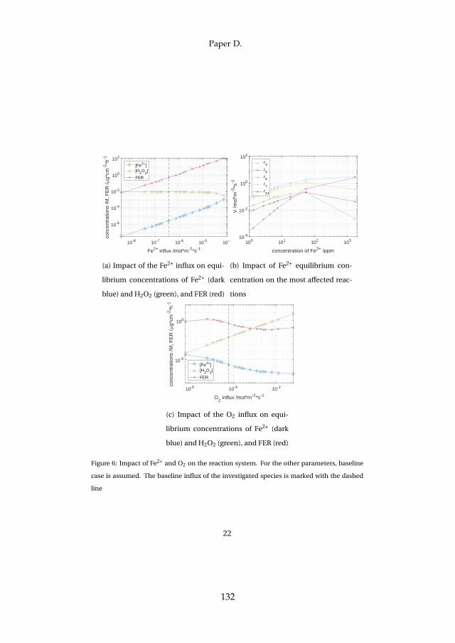
10-8 10-7 10-6 10-5 10-4
Fe2+ influx /mol*m-2*s-1
10-6
10-4
10-2
100
102
conc
entr
atio
ns /M
, FE
R /
g*cm
-2*h
-1
[Fe2+][H
2O
2]
FER
(a) Impact of the Fe2+ influx on equi-
librium concentrations of Fe2+ (dark
blue) and H2O2 (green), and FER (red)
100 101 102 103
concentration of Fe2+ /ppm
10-4
10-2
100
102
V /m
ol*m
-3*s
-1
r3
r5
r6
r7
r14
(b) Impact of Fe2+ equilibrium con-
centration on the most affected reac-
tions
10-6 10-4 10-2
O2 influx /mol*m-2*s-1
10-5
100
conc
entr
atio
ns /M
, FE
R /
g*cm
-2*h
-1
[Fe2+][H
2O
2]
FER
(c) Impact of the O2 influx on equi-
librium concentrations of Fe2+ (dark
blue) and H2O2 (green), and FER (red)
Figure 6: Impact of Fe2+ and O2 on the reaction system. For the other parameters, baselinecase is assumed. The baseline influx of the investigated species is marked with the dashedline
22
Paper D.
132
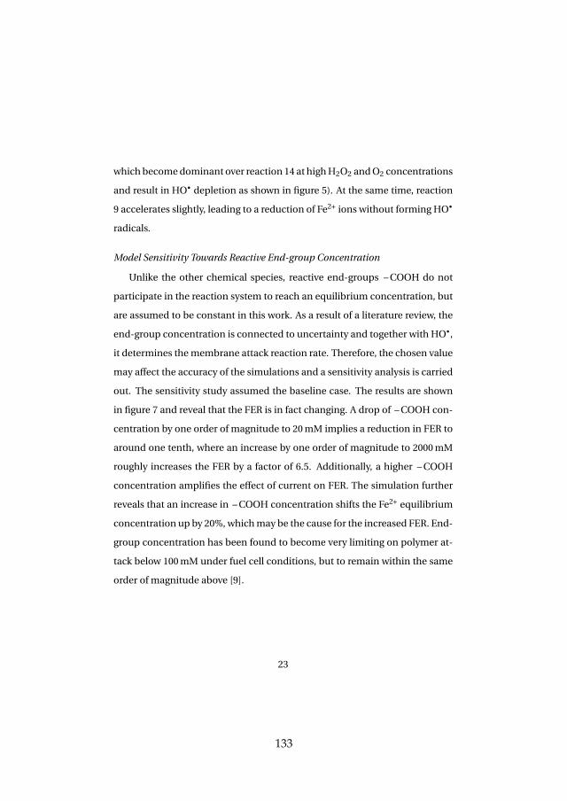
whichbecomedominant over reaction 14 at highH2O2 andO2 concentrationsand result in HO• depletion as shown in figure 5). At the same time, reaction9 accelerates slightly, leading to a reduction of Fe2+ ions without forming HO•
radicals.
Model Sensitivity Towards Reactive End-group Concentration
Unlike the other chemical species, reactive end-groups –COOH do notparticipate in the reaction system to reach an equilibrium concentration, butare assumed to be constant in this work. As a result of a literature review, theend-group concentration is connected to uncertainty and together with HO•,it determines themembrane attack reaction rate. Therefore, the chosen valuemay affect the accuracy of the simulations and a sensitivity analysis is carriedout. The sensitivity study assumed the baseline case. The results are shownin figure 7 and reveal that the FER is in fact changing. A drop of –COOH con-centration by one order of magnitude to 20 mM implies a reduction in FER toaround one tenth, where an increase by one order of magnitude to 2000 mM
roughly increases the FER by a factor of 6.5. Additionally, a higher –COOHconcentration amplifies the effect of current on FER. The simulation furtherreveals that an increase in –COOH concentration shifts the Fe2+ equilibriumconcentration up by 20%, whichmay be the cause for the increased FER. End-group concentration has been found to become very limiting on polymer at-tack below 100 mM under fuel cell conditions, but to remain within the sameorder of magnitude above [9].
23
133
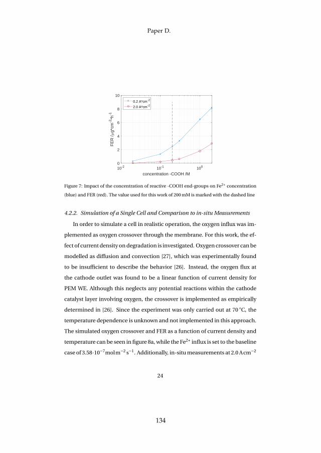
10-2 10-1 100
concentration -COOH /M
0
2
4
6
8
10
FE
R /
g*cm
-2*h
-1
0.2 A*cm-2
2.0 A*cm-2
Figure 7: Impact of the concentration of reactive -COOH end-groups on Fe2+ concentration(blue) and FER (red). The value used for this work of 200 mM is marked with the dashed line
4.2.2. Simulation of a Single Cell and Comparison to in-situ Measurements
In order to simulate a cell in realistic operation, the oxygen influx was im-plemented as oxygen crossover through the membrane. For this work, the ef-fect of currentdensity ondegradation is investigated. Oxygencrossover canbemodelled as diffusion and convection [27], which was experimentally foundto be insufficient to describe the behavior [26]. Instead, the oxygen flux atthe cathode outlet was found to be a linear function of current density forPEM WE. Although this neglects any potential reactions within the cathodecatalyst layer involving oxygen, the crossover is implemented as empiricallydetermined in [26]. Since the experiment was only carried out at 70 C, thetemperature dependence is unknown and not implemented in this approach.The simulated oxygen crossover and FER as a function of current density andtemperature can be seen in figure 8a, while the Fe2+ influx is set to the baselinecase of 3.58·10−7molm−2 s−1. Additionally, in-situmeasurements at 2.0 Acm−2
24
Paper D.
134
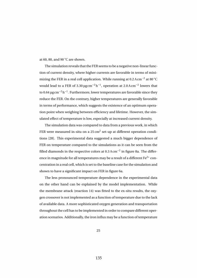
at 60, 80, and 90 C are shown.The simulation reveals that theFERseems tobeanegativenon-linear func-
tion of current density, where higher currents are favorable in terms of mini-mizing the FER in a real cell application. While running at 0.2 Acm−2 at 80 C
would lead to a FER of 3.30µgcm−2 h−1, operation at 2.0 Acm−2 lowers thatto 0.64µgcm−2 h−1. Furthermore, lower temperatures are favorable since theyreduce the FER. On the contrary, higher temperatures are generally favorablein terms of performance, which suggests the existence of an optimum opera-tion point when weighing between efficiency and lifetime. However, the sim-ulated effect of temperature is low, especially at increased current density.
The simulation data was compared to data from a previous work, in whichFER were measured in-situ on a 25 cm2 set-up at different operation condi-tions [28]. This experimental data suggested a much bigger dependence ofFER on temperature compared to the simulations as it can be seen from thefilled diamonds in the respective colors at 0.3 Acm−2 in figure 8a. The differ-ence inmagnitude for all temperaturesmay be a result of a different Fe2+ con-centration in a real cell, which is set to the baseline case for the simulation andshown to have a significant impact on FER in figure 6a.
The less pronounced temperature dependence in the experimental dataon the other hand can be explained by the model implementation. Whilethe membrane attack (reaction 14) was fitted to the ex-situ results, the oxy-gen crossover is not implemented as a function of temperature due to the lackof available data. Amore sophisticated oxygen generation and transportationthroughout the cell has to be implemented in order to compare different oper-ation scenarios. Additionally, the iron influxmay be a function of temperature
25
135
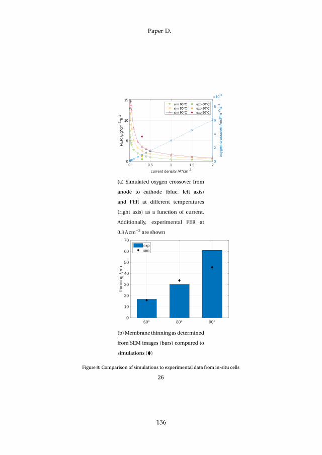
0 0.5 1 1.5 2
current density /A*cm-2
0
5
10
15
FE
R /
g*cm
-2*h
-1
0
2
4
6
8
oxyg
en c
ross
over
/mol
*m-2
*s-1
10-5
sim 60°Csim 80°Csim 90°C
exp 60°Cexp 80°Cexp 90°C
(a) Simulated oxygen crossover from
anode to cathode (blue, left axis)
and FER at different temperatures
(right axis) as a function of current.
Additionally, experimental FER at
0.3 Acm−2 are shown
60° 80° 90°0
10
20
30
40
50
60
70
thin
ning
/m
expsim
(b)Membrane thinningasdetermined
from SEM images (bars) compared to
simulations ()
Figure 8: Comparison of simulations to experimental data from in-situ cells
26
Paper D.
136
if assumingcorrosionofbalanceofplant components as a source. Both factorsmay increase the FER at elevated temperatures. For the sake of completeness,the experimental in-situ data was fitted to the Arrhenius equation, which re-sulted in 79 kJmol−1 and 4.04 ·1018 for activation energy and frequency factorfor reaction 14, respectively. The activation energy formembrane degradationreaction has previously been reported as around 70 kJmol−1 [9].
4.2.3. Simulated Membrane Thinning Through Fluoride Emission
Membrane thinning was evaluated experimentally in a previous work bymeansof scanningelectronmicroscopy (SEM)after500 h for several operationconditions [28]. Thevalues for three temperatures togetherwith the respectivesimulated thinning according to equation IX is presented in figure 8b. Themodel fitting factor, fF,loss was set to 20.8 [12] for all simulations. The factortakes into account, that not all fluoride ions are captured in the outlet effluentwater. It furthermore accounts for fluorine losswithin polymer fragments thatcannot be detected by an ion-selective electrode as used in this experimentalapproach. As a rough estimation, fluorine emission was found up to 6 timeshigher compared to fluoride [20].
The simulation shows fairly good fit at 60 C and 80 C with an error of 6%and 11%, but underestimates thinning at 90 C by 25%. Given the uncertain-ties throughout the several assumptionsmade, these numbers are consideredacceptable as a first evaluation of the effect of the operation mode on mem-brane degradation. Due to the underestimation of fluoride emission at 90 C,the thinning is also underestimated. As a result, the fitting factor fF,loss couldbe empirically adjusted to the measured dataset.
27
137
5. Conclusion
The influence of hydrogen peroxide and iron ions on fluoride emissionhavebeen investigated in ex-situ and in-situ experiments, and through a com-putational model. The results show that hydrogen peroxide acts as a requiredprecursor, while iron catalyzes the reaction considerably. However, even inthe absence of iron, a considerable amount of fluoride emission is observedwhen H2O2 is present. This is linked to the ability of other metallic impuritiesto replace iron as a catalyzer of the reaction. However, the origin, magnitude,and location of metal impurities have to be identified.
A model based on a system of 14 reactions was developed to simulate ex-situ and in-situ environments. Temperatures above 80 C as well as low cur-rent operation is highly unfavorable in terms of membrane degradation, asthe fluoride emission increases non-linearly for both. Furthermore, the sim-ulation revealed high dependence of fluoride emission on reactive end-groupconcentration, which is a parameter of high uncertainty. Considering the highamount of uncertainties among the developedmodel, the results are satisfac-tory for the in-situ simulations for temperatures up to 80 C when comparedto experimental data, but underestimate the effect of temperature above that.This is due to the lack of data for the temperature dependence of oxygen per-meation.
Acknowledgement
The authors would like to acknowledge the support by Innovation FundDenmark through the e-STORE project, Grant 4106-00025B.
28
Paper D.
138
References
[1] P. Trinke, B. Bensmann, S. Reichstein, R. Hanke-Rauschenbach, K. Sund-macher, Hydrogen Permeation in PEM Electrolyzer Cells Operated atAsymmetric Pressure Conditions, Journal of The Electrochemical Soci-ety 163 (11) (2016) F3164–F3170. doi:10.1149/2.0221611jes.URL http://jes.ecsdl.org/lookup/doi/10.1149/2.0221611jes
[2] Q. Feng, X. Yuan, G. Liu, B. Wei, Z. Zhang, H. Li, H. Wang, A review ofproton exchange membrane water electrolysis on degradation mecha-nisms andmitigation strategies, Journal of Power Sources 366 (2017) 33–55. doi:10.1016/j.jpowsour.2017.09.006.URL http://dx.doi.org/10.1016/j.jpowsour.2017.09.006
[3] P. S. Ruvinskiy, A. Bonnefont, C. Pham-Huu, E. R. Savinova,Using orderedcarbon nanomaterials for shedding light on the mechanism of the ca-thodic oxygen reduction reaction, Langmuir 27 (14) (2011) 9018–9027.doi:10.1021/la2006343.
[4] K. Barbusinski, Fenton reaction - Controversy concerning the chemistry,Ecological chemistry and engineering S/Chemia i in·zynieria ekolog-iczna S 16 (3) (2009) 347–358.
[5] A. Pozio, R. F. Silva, M. De Francesco, L. Giorgi, Nafion degradation inPEFCs from end plate iron contamination, Electrochimica Acta 48 (11)(2003) 1543–1549. doi:10.1016/S0013-4686(03)00026-4.
[6] R. Borup, J. Meyers, B. Pivovar, Y. S. Kim, R. Mukundan, N. Garland,D. Myers, M. Wilson, F. Garzon, D. Wood, P. Zelenay, K. More, K. Stroh,
29
139
T. Zawodzinski, X. J. Boncella, J. E. Mcgrath, O. M. Inaba, K. Miyatake,M.Hori, K.Ota, Z.Ogumi, S.Miyata, A.Nishikata, Z. Siroma, Y.Uchimoto,K. Yasuda, K.-i. Kimijima, N. Iwashita, Scientific Aspects of Polymer Elec-trolyte Fuel Cell Durability and Degradation, Chemical Reviews (2007)3904–3951.
[7] V. O. Mittal, H. Russell Kunz, J. M. Fenton, Is H[sub 2]O[sub 2] Involvedin the Membrane Degradation Mechanism in PEMFC?, Electrochemicaland Solid-State Letters 9 (6) (2006) A299. doi:10.1149/1.2192696.URL http://esl.ecsdl.org/cgi/doi/10.1149/1.2192696
[8] A. A. Shah, T. R. Ralph, F. C. Walsh, Modeling and Simulation ofthe Degradation of Perfluorinated Ion-Exchange Membranes in PEMFuel Cells, Journal of The Electrochemical Society 156 (4) (2009) B465.doi:10.1149/1.3077573.URL http://jes.ecsdl.org/cgi/doi/10.1149/1.3077573
[9] L. Gubler, S. M. Dockheer, W. H. Koppenol, Radical (HO, H andHOO) Formation and Ionomer Degradation in Polymer Electrolyte FuelCells, Journal of The Electrochemical Society 158 (7) (2011) B755.doi:10.1149/1.3581040.URL http://jes.ecsdl.org/cgi/doi/10.1149/1.3581040
[10] M. Ghelichi, P. E. A. Melchy, M. H. Eikerling, Radically coarse-grained approach to the modeling of chemical degradation in fuel cellionomers, Journal of Physical Chemistry B 118 (38) (2014) 11375–11386.doi:10.1021/jp506333p.
30
Paper D.
140
[11] M. Chandesris, R. Vincent, L. Guetaz, J.-S. Roch, D. Thoby, M. Quinaud,Membrane degradation in PEM fuel cells: From experimental resultsto semi-empirical degradation laws, International Journal of Hydro-genEnergy 42 (12) (2017) 8139–8149. doi:10.1016/j.ijhydene.2017.02.116.URLhttp://linkinghub.elsevier.com/retrieve/pii/S0360319917306249
[12] M. Chandesris, V. Médeau, N. Guillet, S. Chelghoum, D. Thoby, F. Fouda-Onana, Membrane degradation in PEM water electrolyzer: Numericalmodeling and experimental evidence of the influence of temperatureand current density, International Journal of Hydrogen Energy 40 (3)(2015) 1353–1366. doi:10.1016/j.ijhydene.2014.11.111.
[13] H. Liu, F. D. Coms, J. Zhang, H. A. Gasteiger, A. B. Laconti, Chemicaldegradation: Correlations between electrolyzer and fuel cell findings,in: Polymer Electrolyte Fuel Cell Durability, Springer, 2009, pp. 71–118.doi:10.1007/978-0-387-85536-3_5.
[14] F. Fouda-Onana, M. Chandesris, V. Médeau, S. Chelghoum, D. Thoby,N. Guillet, Investigation on the degradation of MEAs for PEM waterelectrolysers part I: Effects of testing conditions on MEA performancesand membrane properties, International Journal of Hydrogen Energy 41(2016) 16627–16636. doi:10.1016/j.ijhydene.2016.07.125.
[15] T. Sugawara, N. Kawashima, T. N. Murakami, Kinetic study of Nafiondegradation by Fenton reaction, Journal of Power Sources 196 (5) (2011)2615–2620. doi:10.1016/j.jpowsour.2010.10.043.URL http://dx.doi.org/10.1016/j.jpowsour.2010.10.043
31
141
[16] V. A. Sethuraman, J. W. Weidner, A. T. Haug, S. Motupally, L. V. Prot-sailo, Hydrogen Peroxide Formation Rates in a PEMFC Anode andCathode, Journal of The Electrochemical Society 155 (1) (2008) B50.doi:10.1149/1.2801980.URL http://jes.ecsdl.org/cgi/doi/10.1149/1.2801980
[17] K. H. Wong, E. Kjeang, Macroscopic In-SituModeling of Chemical Mem-brane Degradation in Polymer Electrolyte Fuel Cells, Journal of the Elec-trochemical Society 161 (9) (2014) F823–F832. doi:10.1149/2.0031409jes.URL http://jes.ecsdl.org/cgi/doi/10.1149/2.0031409jes
[18] T. Xie, C. A. Hayden, A kinetic model for the chemical degrada-tion of perfluorinated sulfonic acid ionomers: Weak end groupsversus side chain cleavage, Polymer 48 (19) (2007) 5497–5506.doi:10.1016/j.polymer.2007.07.043.URL http://dx.doi.org/10.1016/j.polymer.2007.07.043
[19] C. Zhou, M. A. Guerra, Z. M. Qiu, T. A. Zawodzinski, D. A. Schiraldi,Chemical durability studies of perfluorinated sulfonic acid polymers andmodel compounds under mimic fuel cell conditions, Macromolecules40 (24) (2007) 8695–8707. doi:10.1021/ma071603z.
[20] M. Bodner, B. Marius, A. Schenk, V. Hacker, Determining the Total Fluo-rine Emission Rate in Polymer Electrolyte Fuel Cell Effluent Water, ECSTransactions 80 (8) (2017) 559–563.
[21] F. M. Collette, C. Lorentz, G. Gebel, F. Thominette, Hygrothermal ag-
32
Paper D.
142
ing of Nafion®, Journal of Membrane Science 330 (1-2) (2009) 21–29.doi:10.1016/j.memsci.2008.11.048.
[22] A. B. LaConti, M. Hamdan, R. C. McDonald, Mechanisms of membranedegradation, in: HandbookofFuelCells: Fundamentals, Technology, andApplications, JohnWiley and Sons, 2003, pp. 647–663.
[23] M. Inaba,DegradationMechanismofPolymerElectrolyteFuelCells, 14thInternational Conference on the Properties of Water and Steam in Kyoto(2004) 395–402.
[24] S. GOLDSTEIN, D. MEYERSTEIN, G. CZAPSKI, THE FENTONREAGENTS, Free Radical Biology &Medicine 15 (Ii) (1993) 435–445.
[25] Z. Liu, T. Wang, X. Yu, Z. Geng, Y. Sang, H. Liu, In situ alternativeswitching between Ti <sup>4+</sup> and Ti <sup>3+</sup> driven byH <sub>2</sub> O <sub>2</sub> in TiO <sub>2</sub> nanostructures:mechanism of pseudo-Fenton reaction, Materials Chemistry Frontiers1 (10) (2017) 1989–1994. doi:10.1039/C7QM00163K.URL http://xlink.rsc.org/?DOI=C7QM00163K
[26] P. Trinke, B. Bensmann, R.Hanke-Rauschenbach, Experimental evidenceof increasing oxygen crossover with increasing current density duringPEM water electrolysis, Electrochemistry Communications 82 (June)(2017) 98–102. doi:10.1016/j.elecom.2017.07.018.URL http://dx.doi.org/10.1016/j.elecom.2017.07.018
[27] P. Olivier, C. Bourasseau, P. B. Bouamama, Low-temperature electrolysis
33
143
systemmodelling: A review, Renewable and Sustainable Energy Reviews78 (March) (2017) 280–300. doi:10.1016/j.rser.2017.03.099.
[28] S. H. Frensch, F. Fouda-Onana, G. Serre, D. Thoby, S. S. Araya, S. K. Kær,Influenceof theOperationModeonPEMWaterElectrolysisDegradation.Manuscript submitted for publication (2018).
34
Paper D.
144


Steffen fr
enSc
hLifetim
e inveStig
ation
of Pem
eLectr
oLyzer
S un
der
rea
LiStic Lo
ad
Pro
fiLeS
ISSN (online): 2446-1636 ISBN (online): 978-87-7210-354-9
![arXiv:2007.15506v1 [cs.CV] 30 Jul 2020 · allows training the di cult 2.5D and 3D human representations on the simu-lated people domain and generalize well to the in-the-wild domain](https://img.pdfslide.us/doc/110x75/5fdb77869d4fff1bdc520841/arxiv200715506v1-cscv-30-jul-2020-allows-training-the-di-cult-25d-and-3d-human.jpg)


![Model Predictive Compressor Surge Control - TU/e · In Willems [2000] active surge control of a centrifugal compressor is simu- lated and implemented on a gas turbine installation](https://img.pdfslide.us/doc/110x75/5b52daa17f8b9af4408e25ea/model-predictive-compressor-surge-control-tue-in-willems-2000-active-surge.jpg)


![Climatic response to high-latitude volcanic eruptions · 2009-09-24 · eruption of El Chicho´n.Graf and Timmreck [2001] simu-lated the aerosol radiative effects of the Laacher See](https://img.pdfslide.us/doc/110x75/5f590768d30229245175dbd6/climatic-response-to-high-latitude-volcanic-eruptions-2009-09-24-eruption-of-el.jpg)


![CFD Simulation of Dilute Gas-Solid Flow in 90oSquare Bend · both the gas and particle phases. Chu and Yu [10] simu- lated numerically gas solid flow in complex three-di- mensional](https://img.pdfslide.us/doc/110x75/5ed9f82228db2d5ca2492bf1/cfd-simulation-of-dilute-gas-solid-flow-in-90osquare-bend-both-the-gas-and-particle.jpg)