Embed Size (px)
Citation preview
AAE 526: More Linear Programming
Thomas F. Rutherford
Fall Semester, 2019Department of Agricultural and Applied Economics
University of Wisconsin, Madison
September 9, 2019
1 / 59
Outline
• Another LP example
• Linear algebra and indexed GAMS code
• Linear programs in standard form
• Supersize me!
• Visualization
2 / 59

Another Tiny LP
The Wyndor Glass Co. produces high-quality glass products, includingwindows and glass doors. It has three plants. Aluminum frames andhardware are made in Plant 1, wood frames are made in Plant 2 and Plant3 cuts the glass and assembles the products.Profits are 3 for product 1 and 5 per unit of product 2.Because of declining earnings, top management has decided to revamp theproduct line. Unprofitable products are to be discontinued, and productcapacity will be reassigned to launch two new products.
3 / 59

Describe Constraints
The data indicates that each batch of product 1 produced per weekuses 1 hour of production time per week in Plant 1, whereas only 4hours per week are available. The restriction is writtenmathematically as
x1 ≤ 4
Similarly, Plant 2 imposes the restriction
2x2 ≤ 12
The number of hours of production time used per week in Plant 3given x1 and x2 is 3x1 + 2x2 (3 hours of production per batch of good1 and 2 hours per batch of good 2). The available capacity in Plant 3provides the constraint:
3x1 + 2x2 ≤ 18
Finally, production rates cannot be negative, so it is necessary toimpose restrictions x1 ≥ 0 and x2 ≥ 0
4 / 59

Write Down an Algebraic Formulation
maxZ = 3x1 + 5x2
subject to the restrictions
x1 ≤ 42x2 ≤ 12
3x1 +2x2 ≤ 18
andx1 ≥ 0, x2 ≥ 0
5 / 59

6 / 59
Graphical Solution: for Two Variable Problems
This problem has only two dimensions, so a graphical procedure can beemployed. We use label the axes as x1 and x2. The first step is then toidentify on the graph values of (x1, x2) which are feasible (consistent withthe restrictions).
7 / 59

Upper and Lower Bounds
Values of (x1, x2) consistent with the constraints 0 ≤ x1 ≤ 4 and 0 ≤ x2:
8 / 59

The Feasible Region
9 / 59
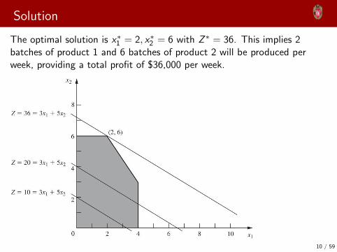
Solution
The optimal solution is x∗1 = 2, x∗2 = 6 with Z ∗ = 36. This implies 2batches of product 1 and 6 batches of product 2 will be produced perweek, providing a total profit of $36,000 per week.
10 / 59

Outline
• Another LP example
• Linear algebra and indexed GAMS code
• Linear programs in standard form
• Supersize me!
• Visualization
11 / 59

Most Practical GAMS Models are Indexed
$TITLE Brewery Profit Maximization
set j Products /lager, ale/
i Ingredients /
malt Malt,
yeast Yeast,
dehops German hops,
wihops Wisconsin hops/;
parameter
p(j) Profit by product /lager 12, ale 9/
s(i) Supply by ingredient /malt 4800, yeast 1750,
dehops 1000, wihops 1750/;
table a(i,j) Requirements
lager ale
malt 4 2
yeast 1 1
dehops 1 0
wihops 0 1;
12 / 59

GAMS Models are Indexed (cont.)
variables Y(j) Production levels,
Z Profit (maximand);
nonnegative variable Y;
equations supply(i) Ingredient supply
profit Defines Z;
supply(i).. sum(j, a(i,j)*Y(j)) =L= s(i);
profit.. Z =E= sum(j, p(j)*Y(j));
MODEL BREWERY /supply, profit/;
solve BREWERY using LP maximizing Z;
13 / 59

Matrix basics
A matrix is an array of numbers. A ∈ Rm×n.
A =
a11 · · · a1n
.... . .
...am1 · · · amn
which has m rows and n columns.
The table statement in GAMS can be used to define a matrix:
set i Row indices /1*3/,
j Column indice /1*2/;
table a(i,j) Matrix with three rows and two columns
1 2
1 0.23 12.3
2 -0.1 2.4
3 3.2 0.1 ;
14 / 59

Table versus Parameter
A matrix may be specified either the table or parameter statement:
set i Row indices /1*3/,
j Column indice /a,b/;
table a(i,j) Matrix with three rows and two columns
a b
1 0.23 12.3
2 -0.1 2.4
3 3.2 0.1 ;
parameter b(i,j) The same matrix in database format /
1.a 0.23
2.a -0.1
3.a 3.2
1.b 12.3
2.b 2.4
3.b 0.1 /;
parameter c(i,j) Check that a=b; c(i,j) = a(i,j) - b(i,j); display c;
---- 22 PARAMETER c check that a=b
( ALL 0.000 )
15 / 59

Matrix Multiplication
Two matrices can be multiplied if their inner dimensions agree. In matrixnotation (MATLAB style):
C︸︷︷︸(m×p)
= A︸︷︷︸(m×n)
B︸︷︷︸(n×p)
In detached coefficient notation (GAMS style) we write:
cij =∑k
aikbkj
In GAMS syntax, we have:
c(i,j) = sum(k, a(i,k) * b(k,j));
16 / 59
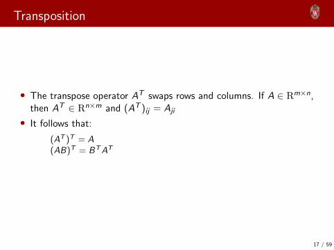
Transposition
• The transpose operator AT swaps rows and columns. If A ∈ Rm×n,then AT ∈ Rn×m and (AT )ij = Aji
• It follows that:
(AT )T = A(AB)T = BTAT
17 / 59

Linear and affine functions
• A function f (x1, . . . , xm) is linear in the variables x1, . . . , xm if thereexists constants a1, . . . , am such that
f (x1, . . . , xm) = a1x1 + . . .+ amxm =∑i
aixi = aT x
• A function f (x1, . . . , xm) is affine in the variables x1, . . . , xm if thereexists constants b, a1, . . . , am such that
f (x1, . . . , xm) = ba1x1 + . . .+ amxm = b +∑i
aixi = b + aT x
• Examples:
1 3x − y is linear in (x , y).2 2xy + 1 is affine in x and y , but not in (x , y).3 x2 + y2 is neither linear nor affine.
18 / 59
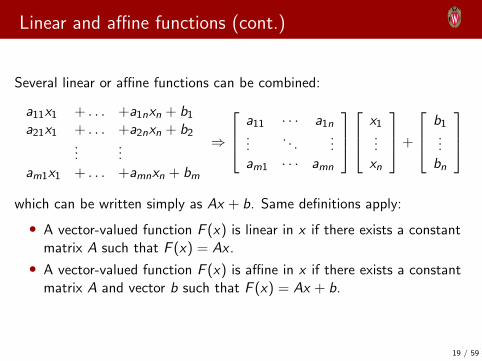
Linear and affine functions (cont.)
Several linear or affine functions can be combined:
a11x1 + . . . +a1nxn + b1
a21x1 + . . . +a2nxn + b2...
...am1x1 + . . . +amnxn + bm
⇒
a11 · · · a1n...
. . ....
am1 · · · amn
x1
...xn
+
b1...bn
which can be written simply as Ax + b. Same definitions apply:
• A vector-valued function F (x) is linear in x if there exists a constantmatrix A such that F (x) = Ax .
• A vector-valued function F (x) is affine in x if there exists a constantmatrix A and vector b such that F (x) = Ax + b.
19 / 59
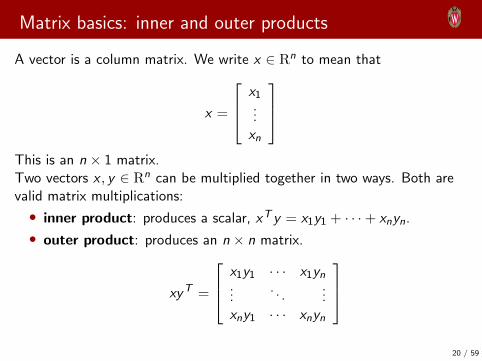
Matrix basics: inner and outer products
A vector is a column matrix. We write x ∈ Rn to mean that
x =
x1...xn
This is an n × 1 matrix.Two vectors x , y ∈ Rn can be multiplied together in two ways. Both arevalid matrix multiplications:
• inner product: produces a scalar, xT y = x1y1 + · · ·+ xnyn.
• outer product: produces an n × n matrix.
xyT =
x1y1 · · · x1yn...
. . ....
xny1 · · · xnyn
20 / 59
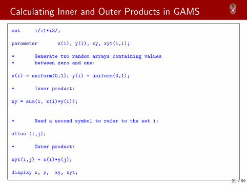
Calculating Inner and Outer Products in GAMS
set i/i1*i3/;
parameter x(i), y(i), xy, xyt(i,i);
* Generate two random arrays containing values
* between zero and one:
x(i) = uniform(0,1); y(i) = uniform(0,1);
* Inner product:
xy = sum(i, x(i)*y(i));
* Need a second symbol to refer to the set i:
alias (i,j);
* Outer product:
xyt(i,j) = x(i)*y(j);
display x, y, xy, xyt;
21 / 59
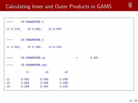
Calculating Inner and Outer Products in GAMS
---- 23 PARAMETER x
i1 0.172, i2 0.843, i3 0.550
---- 23 PARAMETER y
i1 0.301, i2 0.292, i3 0.224
---- 23 PARAMETER xy = 0.421
---- 23 PARAMETER xyt
i1 i2 i3
i1 0.052 0.050 0.038
i2 0.254 0.246 0.189
i3 0.166 0.161 0.123
22 / 59

Outline
• Another LP example
• Linear algebra and indexed GAMS code
• Linear programs in standard form
• Supersize me!
• Visualization
23 / 59
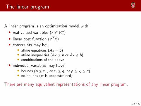
The linear program
A linear program is an optimization model with:
• real-valued variables (x ∈ Rn)
• linear cost function (cT x)• constraints may be:
• affine equations (Ax = b)• affine inequalities (Ax ≤ b or Ax ≥ b)• combinations of the above
• individual variables may have:• bounds (p ≤ xi , or xi ≤ q, or p ≤ xi ≤ q)• no bounds (xi is unconstrained)
There are many equivalent representations of any linear program.
24 / 59
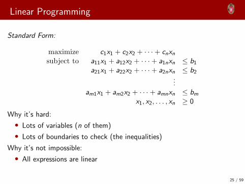
Linear Programming
Standard Form:
maximize c1x1 + c2x2 + · · ·+ cnxnsubject to a11x1 + a12x2 + · · ·+ a1nxn ≤ b1
a21x1 + a22x2 + · · ·+ a2nxn ≤ b2...
am1x1 + am2x2 + · · ·+ amnxn ≤ bmx1, x2, . . . , xn ≥ 0
Why it’s hard:
• Lots of variables (n of them)
• Lots of boundaries to check (the inequalities)
Why it’s not impossible:
• All expressions are linear
25 / 59
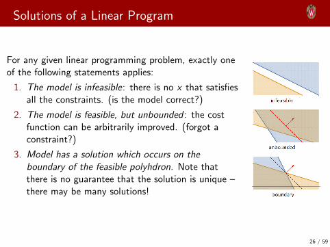
Solutions of a Linear Program
For any given linear programming problem, exactly oneof the following statements applies:
1. The model is infeasible: there is no x that satisfiesall the constraints. (is the model correct?)
2. The model is feasible, but unbounded : the costfunction can be arbitrarily improved. (forgot aconstraint?)
3. Model has a solution which occurs on theboundary of the feasible polyhdron. Note thatthere is no guarantee that the solution is unique –there may be many solutions!
26 / 59
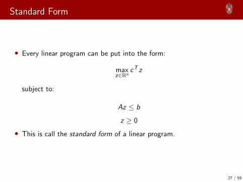
Standard Form
• Every linear program can be put into the form:
maxz∈Rn
cT z
subject to:
Az ≤ b
z ≥ 0
• This is call the standard form of a linear program.
27 / 59
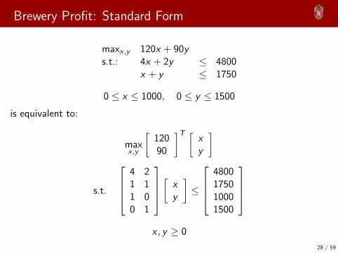
Brewery Profit: Standard Form
maxx ,y 120x + 90ys.t.: 4x + 2y ≤ 4800
x + y ≤ 1750
0 ≤ x ≤ 1000, 0 ≤ y ≤ 1500
is equivalent to:
maxx ,y
[12090
]T [xy
]
s.t.
4 21 11 00 1
[ xy
]≤
4800175010001500
x , y ≥ 0
28 / 59
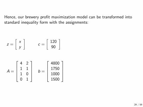
Hence, our brewery profit maximization model can be transformed intostandard inequality form with the assignments:
z =
[xy
]c =
[12090
]
A =
4 21 11 00 1
b =
4800175010001500
29 / 59

Applications of Linear Programming
A partial list, taken from Ferris et al., Chapter 1:
• Resoure allocation
• The diet problem
• Linear surface fitting
• Load balancing
• Classification
• Minimum cost network flow
• ...
30 / 59
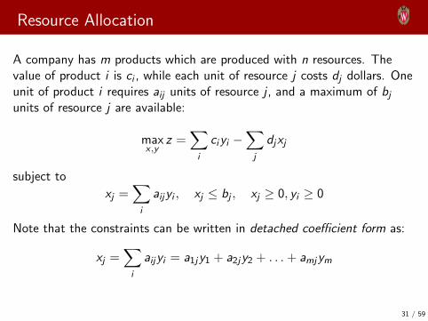
Resource Allocation
A company has m products which are produced with n resources. Thevalue of product i is ci , while each unit of resource j costs dj dollars. Oneunit of product i requires aij units of resource j , and a maximum of bjunits of resource j are available:
maxx ,y
z =∑i
ciyi −∑j
djxj
subject to
xj =∑i
aijyi , xj ≤ bj , xj ≥ 0, yi ≥ 0
Note that the constraints can be written in detached coefficient form as:
xj =∑i
aijyi = a1jy1 + a2jy2 + . . .+ amjym
31 / 59

The Diet Problem
Given the prices pj of food type j , the content of nutrient i in food j (aij)and the dietary requirement of nutrient i , bi , solve:
minx
z =∑j
pjxj
subject to ∑j
aijxj ≥ bi , ∀i
xj ≥ 0
32 / 59

Linear Surface Fitting
Given a set of observations A = [aij ] and bi . Find weights on the columns of Aand a scalar constant γ which best “predicts” the value of b on the basis ofobservations aij , assuming a linear model:
minx,γ
m∑i=1
∣∣∣∣∣∣∑j
aijxj + γ − bi
∣∣∣∣∣∣or, equivalently
minx,γ,y
z =∑i
yi
subject to
−yi ≤∑j
aijxj + γ − bi ≤ yi
Note that the constraint ensures that each yi is no smaller than the absolutevalue |
∑j aijxj + γ − bi |.
33 / 59
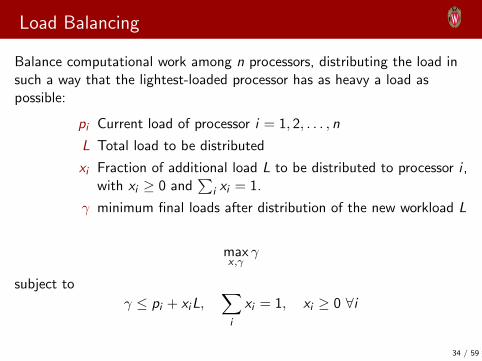
Load Balancing
Balance computational work among n processors, distributing the load insuch a way that the lightest-loaded processor has as heavy a load aspossible:
pi Current load of processor i = 1, 2, . . . , n
L Total load to be distributed
xi Fraction of additional load L to be distributed to processor i ,with xi ≥ 0 and
∑i xi = 1.
γ minimum final loads after distribution of the new workload L
maxx ,γ
γ
subject to
γ ≤ pi + xiL,∑i
xi = 1, xi ≥ 0 ∀i
34 / 59

Outline
• Another LP example
• Linear algebra and indexed GAMS code
• Linear programs in standard form
• Supersize me!
• Visualization
35 / 59
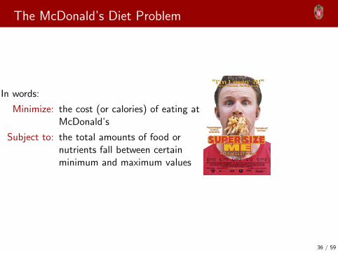
The McDonald’s Diet Problem
In words:
Minimize: the cost (or calories) of eating atMcDonald’s
Subject to: the total amounts of food ornutrients fall between certainminimum and maximum values
36 / 59
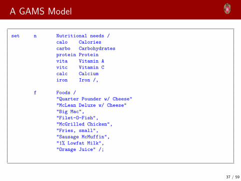
A GAMS Model
set n Nutritional needs /
calo Calories
carbo Carbohydrates
protein Protein
vita Vitamin A
vitc Vitamin C
calc Calcium
iron Iron /,
f Foods /
"Quarter Pounder w/ Cheese"
"McLean Deluxe w/ Cheese"
"Big Mac",
"Filet-O-Fish",
"McGrilled Chicken",
"Fries, small",
"Sausage McMuffin",
"1% Lowfat Milk",
"Orange Juice" /;
37 / 59
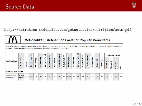
Source Data
http://nutrition.mcdonalds.com/getnutrition/nutritionfacts.pdf
38 / 59
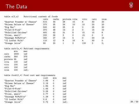
The Data
table a(f,n) Nutritional content of foods
calo carbo protein vita vitc calc iron
"Quarter Pounder w/ Cheese" 510 34 28 15 6 30 20
"McLean Deluxe w/ Cheese" 370 35 24 15 10 20 20
"Big Mac" 500 42 25 6 2 25 20
"Filet-O-Fish" 370 38 14 2 0 15 10
"McGrilled Chicken" 400 42 31 8 15 15 8
"Fries, small" 220 26 3 0 15 0 2
"Sausage McMuffin" 345 27 15 4 0 20 15
"1% Lowfat Milk" 110 12 9 10 4 30 0
"Orange Juice" 80 20 1 2 120 2 2;
table nutr(n,*) Nutrient requirements
min max
calo 2000 inf
carbo 350 375
protein 55 inf
vita 100 inf
vitc 100 inf
calc 100 inf
iron 100 inf;
table food(f,*) Food cost and requirements
cost min max
"Quarter Pounder w/ Cheese" 1.84 0 inf
"McLean Deluxe w/ Cheese" 2.19 0 inf
"Big Mac" 1.84 0 inf
"Filet-O-Fish" 1.44 0 inf
"McGrilled Chicken" 2.29 0 inf
"Fries, small" 0.77 0 inf
"Sausage McMuffin" 1.29 0 inf
"1% Lowfat Milk" 0.6 0 inf
"Orange Juice" 0.72 0 inf; 39 / 59

Model Equations
nonnegative
variables Y(n) Nutritional content
X(f) Purchased quantity;
free
variable COST Total cost;
equations ydef, objdef;
ydef(n).. Y(n) =e= sum(f, X(f)*a(f,n));
objdef.. COST =e= sum(f, X(f) * food(f,"cost"));
model mincost /ydef, objdef /;
Y.LO(n) = nutr(n,"min"); Y.UP(n) = nutr(n,"max");
X.LO(f) = food(f,"min"); X.UP(f) = food(f,"max");
40 / 59

First Run
solve mincost using lp minimizing COST;
* Generate reports of the menu and diet:
parameter menu Resulting menu,;
menu("Cost","MinCost") = COST.L;
menu("Calories","MinCost") = Y.L("calo");
menu("ModelStat","MinCost") = mincost.modelstat;
menu("solvestat","MinCost") = mincost.solvestat;
menu(f,"MinCost") = X.L(f);
display menu;
41 / 59

First Run
MinCost
Cost 14.856
Calories 3965.369
Quarter Pounder w/ Cheese 4.385
Fries, small 6.148
1% Lowfat Milk 3.422
Cheap, but4000 calories!
42 / 59

Second Run
Put an upper bound on calories.
Y.UP("calo") = 2500;
solve mincost using lp minimizing COST;
Calories are down, cost is up and the diet looks better.
MinCost Cal2500
Cost 14.856 16.671
Calories 3965.369 2500.000
Quarter Pounder w/ Cheese 4.385 0.232
McLean Deluxe w/ Cheese 3.855
Fries, small 6.148
1% Lowfat Milk 3.422 2.043
Orange Juice 9.134
43 / 59

Third Run
Try for a 2000 calorie diet.
Y.UP("calo") = 2000;
solve mincost using lp minimizing COST;
Not possible!
MODEL mincost OBJECTIVE C
TYPE LP DIRECTION MINIMIZE
SOLVER CPLEX FROM LINE 121
**** SOLVER STATUS 1 Normal Completion
**** MODEL STATUS 4 Infeasible
**** OBJECTIVE VALUE 0.9121
44 / 59

Minimize calories, ignoring cost.
variable CALO Objective value -- calories;
equation objcalo Objective -- minimize calories;
objcalo.. CALO =e= Y("calo");
model mincal /ydef, objdef, objcalo/;
solve mincal using lp minimizing CALO;
Minimum calories is 2467 at a cost of $16.75:
MinCost Cal2500 MinCal
Cost 14.856 16.671 16.745
Calories 3965.369 2500.000 2466.981
Quarter Pounder w/ Cheese 4.385 0.232
McLean Deluxe w/ Cheese 3.855 4.088
Fries, small 6.148
1% Lowfat Milk 3.422 2.043 2.044
Orange Juice 9.134 9.119
45 / 59

Add some variety
X.UP(f) = 2;
solve mincost using lp minimizing COST;
More intersting cuisine. Cost is up a bit, calories are down relative to originalsolution.
MinCost MinCal MinCostV
Cost 14.856 16.745 16.766
Calories 3965.369 2466.981 3798.077
Quarter Pounder w/ Cheese 4.385 2.000
McLean Deluxe w/ Cheese 4.088 2.000
Big Mac 2.000
Fries, small 6.148 1.423
Sausage McMuffin 1.000
1% Lowfat Milk 3.422 2.044 2.000
Orange Juice 9.119 2.000
46 / 59

Keep variety but minimize calories
X.UP(f) = 2;
solve mincal using lp minimizing COST;
Almost 3500 calories. Wow!
MinCost MinCal MinCostV MinCalV
Cost 14.856 16.745 16.766 17.248
Calories 3965.369 2466.981 3798.077 3488.287
Quarter Pounder w/ Cheese 4.385 2.000 1.952
McLean Deluxe w/ Cheese 4.088 2.000 2.000
Big Mac 2.000
Filet-O-Fish 0.359
McGrilled Chicken 2.000
Fries, small 6.148 1.423 2.000
Sausage McMuffin 1.000
1% Lowfat Milk 3.422 2.044 2.000 2.000
Orange Juice 9.119 2.000 2.000
47 / 59
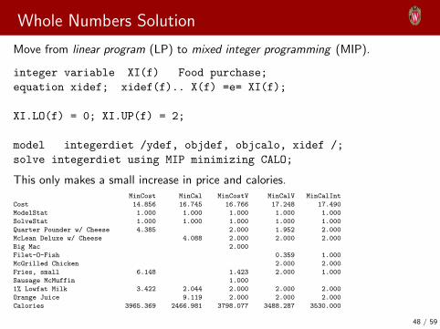
Whole Numbers Solution
Move from linear program (LP) to mixed integer programming (MIP).
integer variable XI(f) Food purchase;
equation xidef; xidef(f).. X(f) =e= XI(f);
XI.LO(f) = 0; XI.UP(f) = 2;
model integerdiet /ydef, objdef, objcalo, xidef /;
solve integerdiet using MIP minimizing CALO;
This only makes a small increase in price and calories.MinCost MinCal MinCostV MinCalV MinCalInt
Cost 14.856 16.745 16.766 17.248 17.490
ModelStat 1.000 1.000 1.000 1.000 1.000
SolveStat 1.000 1.000 1.000 1.000 1.000
Quarter Pounder w/ Cheese 4.385 2.000 1.952 2.000
McLean Deluxe w/ Cheese 4.088 2.000 2.000 2.000
Big Mac 2.000
Filet-O-Fish 0.359 1.000
McGrilled Chicken 2.000 2.000
Fries, small 6.148 1.423 2.000 1.000
Sausage McMuffin 1.000
1% Lowfat Milk 3.422 2.044 2.000 2.000 2.000
Orange Juice 9.119 2.000 2.000 2.000
Calories 3965.369 2466.981 3798.077 3488.287 3530.000
48 / 59
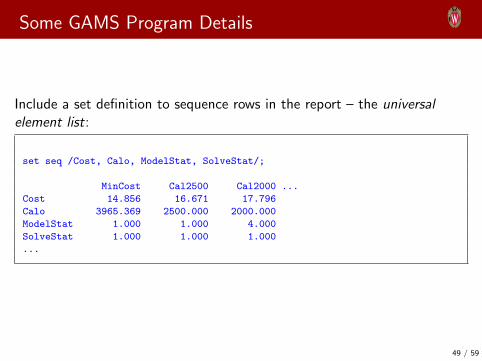
Some GAMS Program Details
Include a set definition to sequence rows in the report – the universalelement list:
set seq /Cost, Calo, ModelStat, SolveStat/;
MinCost Cal2500 Cal2000 ...
Cost 14.856 16.671 17.796
Calo 3965.369 2500.000 2000.000
ModelStat 1.000 1.000 4.000
SolveStat 1.000 1.000 1.000
...
49 / 59
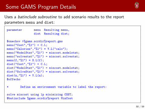
Some GAMS Program Details
Uses a batinclude subroutine to add scenario results to the reportparameters menu and diet:
parameter menu Resulting menu,
diet Resulting diet;
$onechov >%gams.scrdir%report.gms
menu("Cost","%1") = C.L;
menu("Calories","%1") = Y.L("calo");
menu("ModelStat","%1") = mincost.modelstat;
menu("solvestat","%1") = mincost.solvestat;
menu(f,"%1") = X.L(f);
diet("Cost","%1") = C.L;
diet("ModelStat","%1") = mincost.modelstat;
diet("SolveStat","%1") = mincost.solvestat;
diet(n,"%1") = Y.L(n);
$offecho
* Define an environment variable to label the report:
solve mincost using lp minimizing COST;
$batinclude %gams.scrdir%report MinCost
50 / 59
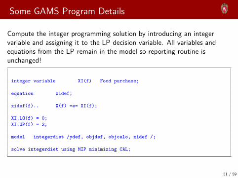
Some GAMS Program Details
Compute the integer programming solution by introducing an integervariable and assigning it to the LP decision variable. All variables andequations from the LP remain in the model so reporting routine isunchanged!
integer variable XI(f) Food purchase;
equation xidef;
xidef(f).. X(f) =e= XI(f);
XI.LO(f) = 0;
XI.UP(f) = 2;
model integerdiet /ydef, objdef, objcalo, xidef /;
solve integerdiet using MIP minimizing CAL;
51 / 59

Outline
• Another LP example
• Linear algebra and indexed GAMS code
• Linear programs in standard form
• Supersize me!
• Visualization
52 / 59

Recall the Brewery Profit Model
maxx ,y
120x + 90y
subject to:4x + 2y ≤ 4800
x + y ≤ 1750
0 ≤ x ≤ 1000
0 ≤ y ≤ 1500
In which:
x : number of batches of lager produced
y : number of batches of ales produced
53 / 59
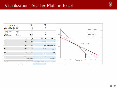
Visualization: Scatter Plots in Excel
54 / 59
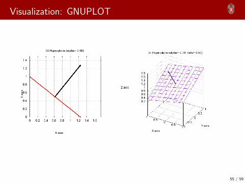
Visualization: GNUPLOT
55 / 59

Visualization: GNUPLOT
0
500
1000
1500
2000
2500
0 200 400 600 800 1000 1200 1400
feasible region
Profit(650,1100)=17700
bat
ches
ofal
e(Y
)
batches of lager (X )
yeastmalt
isoprofit
56 / 59
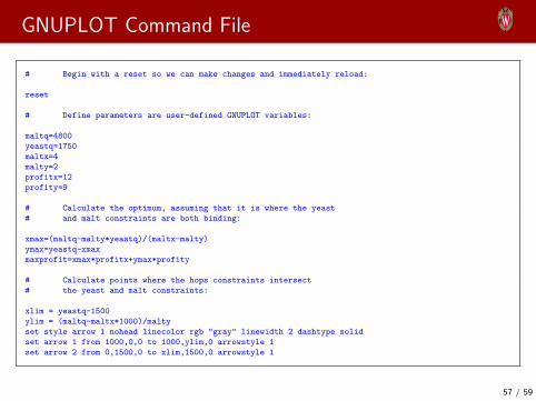
GNUPLOT Command File
# Begin with a reset so we can make changes and immediately reload:
reset
# Define parameters are user-defined GNUPLOT variables:
maltq=4800
yeastq=1750
maltx=4
malty=2
profitx=12
profity=9
# Calculate the optimum, assuming that it is where the yeast
# and malt constraints are both binding:
xmax=(maltq-malty*yeastq)/(maltx-malty)
ymax=yeastq-xmax
maxprofit=xmax*profitx+ymax*profity
# Calculate points where the hops constraints intersect
# the yeast and malt constraints:
xlim = yeastq-1500
ylim = (maltq-maltx*1000)/malty
set style arrow 1 nohead linecolor rgb "gray" linewidth 2 dashtype solid
set arrow 1 from 1000,0,0 to 1000,ylim,0 arrowstyle 1
set arrow 2 from 0,1500,0 to xlim,1500,0 arrowstyle 1
57 / 59

GNUPLOT Command File (cont)
# Define linear functions representing the yeast and malt
# constraints as well as the isoprofit line at the optimal
# point:
yeast(x)=yeastq-x
malt(x)=(maltq-maltx*x)/malty
isoprofit(x) = ymax-profitx*(x-xmax)/profity
# Set up axes:
set xrange [0:1500]
set yrange [0:2500]
set ylabel ’batches of ale (y)’ offset -1,0
set xlabel ’batches lager (x)’ offset 0,-1
set xtics axis
set ytics axis
unset border
set arrow 3 from 0,0 to 1450,0 linestyle 1
set arrow 4 from 0,0 to 0,2550 linestyle 1
# Label the feasible region:
set label "feasible region" at 200,500
# Put a black circle at the optimum:
optimum = sprintf(’(%.f,%.f)’,xmax,ymax)
set label optimum at xmax+30,ymax+30
set object circle at xmax,ymax front size 6 \
fillstyle solid 1 fillcolor rgb "black"58 / 59

GNUPLOT Command File (cont)
# Generate a data file with extreme points of the feasible region:
set print "feasible.dat"
print sprintf(’%.f %.f’,0,0)
print sprintf(’%.f %.f’,0,1500)
print sprintf(’%.f %.f’,xlim, 1500)
print sprintf(’%.f %.f’,xmax, ymax)
print sprintf(’%.f %.f’,1000, ylim)
print sprintf(’%.f %.f’,1000, 0)
unset print
# Define the style to be used for "filledcurves" to denote the
# feasible region:
set style fill transparent solid 0.2 noborder
set style line 1 linecolor "black" linewidth 2 dashtype 1
set style line 2 linecolor "forest-green" linewidth 2 dashtype 1
set style line 3 linecolor "red" linewidth 2 dashtype 2
plot yeast(x) ls 1, malt(x) ls 2, isoprofit(x) ls 3, \
’feasible.dat’ using 1:2 with filledcurves below notitle
59 / 59