AAAI Proceedings Template - users.dsic.upv.esusers.dsic.upv.es/.../coplas'10-proceedings.pdf · COPLAS 2010 Proceedings of the Workshop on Constraint Satisfaction Techniques for Planning

COPLAS 2010 Proceedings of the Workshop on

Constraint Satisfaction Techniques for Planning and Scheduling Problems

Toronto, Canada May 12, 2010

Edited by Miguel A. Salido, Roman Barták and Neil Yorke-Smith

Preface The areas of AI planning and scheduling have seen important advances thanks to application of constraint satisfaction and optimisation techniques. Efficient constraint handling is important for real-world problems in planning, scheduling, and resource allocation to competing goal activities over time in the presence of complex state-dependent constraints. Approaches to these problems must integrate resource allocation and plan synthesis capabilities. We need to manage complex problems where planning, scheduling, and constraint satisfaction must be interrelated, which entail a great potential of application. This workshop, the fifth in a series, aims at providing a forum for meeting and exchanging ideas and novel works in the field of AI planning, scheduling, and constraint satisfaction techniques, and the many relationships that exist among them. In fact, most of the accepted papers are based on combined approaches of constraint satisfaction for planning, scheduling, and mixing planning and scheduling. The workshop was held in May 2010 in Toronto, Canada during the International Conference on Automated Planning and Scheduling (ICAPS'10). COPLAS is ranked as CORE B in ERA Conference Ranking. All the submissions were reviewed by at least two anonymous referees from the program committee, who decided to accept eight papers for oral presentation in the workshop. The papers provide a mix of constraint satisfaction and optimisation techniques for planning, scheduling, and related topics, and their applications to real-world problems. We hope that the ideas and approaches presented in the papers and presentations will lead to a valuable discussion and will inspire future research and developments for all the workshop participants. The Organizing Committee. May, 2010

Miguel A. Salido Roman Barták Neil Yorke-Smith

Organization

Organizing Committee Miguel A. Salido, Universidad Politécnica de Valencia, Spain Roman Barták, Charles University, Czech Republic Neil Yorke-Smith, American University of Beirut, Lebanon, and SRI International, USA

Programme Committee Federico Barber, Universidad Politécnica de Valencia, Spain

Roman Barták, Charles University, The Czech Republic

Amedeo Cesta, ISTC-CNR, Italy

Minh Binh Do, PARC, USA

Enrico Giunchiglia, Universita di Genova, Italy

Peter Jarvis, NASA Ames Research Center, USA

Michela Milano, Università di Bologna, Italy

Alexander Nareyek, National University of Singapore, Singapore

Eva Onaindía, Universidad Politécnica de Valencia, Spain

Nicola Policella, European Space Agency, Germany

Hana Rudová, Masaryk University, The Czech Republic

Francesca Rossi, University of Padova, Italy

Migual A. Salido, Universidad Politecnica Valencia, Spain

Pascal Van Hentenryck, Brown University, USA

Gérard Verfaillie, ONERA, Centre de Toulouse, France

Vincent Vidal, CRIL-IUT, France

Petr Vilím, ILOG, France

Toby Walsh, University of New South Wales, Australia and NICTA, Australia

Neil Yorke-Smith, American University of Beirut, Lebanon and SRI International, USA

Content AI Planning with Time and Resource Constraints Filip Dvořák and Roman Barták ....................................................................................................... 5 Cost-Optimal Planning usingWeighted MaxSAT Nathan Robinson, Charles Gretton, Duc-Nghia Pham and Abdul Sattar ...................................... 14 A Pseudo-Boolean approach for Solving Planning Problems with IPC Simple Preferences Enrico Giunchiglia and Marco Maratea ........................................................................................ 23 Tabu Search and Genetic Algorithm for Scheduling with Total Flow Time Minimization Miguel A. Gonzalez, Camino R. Vela, Marıa Sierra and Ramiro Varela ....................................... 33 Casting Project Scheduling with Time Windows as a DTP Angelo Oddi, Riccardo Rasconi and Amedeo Cesta ....................................................................... 42 Weak and Dynamic Controllability of Temporal Problems with Disjunctions and Uncertainty K. Brent Venable, Michele Volpato, Bart Peintner and Neil Yorke-Smith ..................................... 50 On two perspectives in decomposing constraint systems. Equivalences and computational properties Cees Witteveen, Wiebe van der Hoek and Michael Wooldridge ..................................................... 60 A Filtering Technique for the Railway Scheduling Problem Marlene Arangu, Miguel A. Salido and Federico Barber ............................................................... 68

AI Planning with Time and Resource Constraints

Department of Theoretical Computer Science and Mathematical LogicFaculty of Mathematics and Physics, Charles University in Prague

Malostranské nám. 2/25, 118 00 Praha 1, Czech [email protected], [email protected]

AbstractIntroduction of explicit time and resources into planning that typically focuses on causal relations between actions is an important step towards modelling real-life problems. In this paper we propose a suboptimal domain-independent planning system Filuta that focuses on planning, where time plays a major role and resources are constrained. We benchmark Filuta on the planning problems from the International Planning Competition (IPC) 2008 and compare our results with the competition participants.

IntroductionIn this paper we focus on fully observable, deterministic temporal planning with resources (Ghallab, Nau, & Traverso, 2004). In particular, the world state is specified using a set of multi-valued state-variables where different states are distinguished by different values assigned to the state-variables. The values of all state-variables are specified for the initial state, while the goal state is specified by required values of certain state-variables. Actions have known duration, require particular values of certain state-variables for execution (precondition) and change values of some state-variables at some time point of execution (effect). Resource constraints can then be naturally described using the state-variables, where the value is changed relatively (increased or decreased) rather than being set absolutely. The planning task is to find a set of actions allocated to time such that the time evolution of state-variables is feasible (each state-variable has a unique value at each time point and this value is consistent with actions being executed at this point) and the final values of state-variables satisfy the goal condition. The quality of plan is measured by time needed to reach the goal state –makespan. Plans with a smaller makespan are preferred. Filuta is a sub-optimal domain-independent planning system that solves the above sketched planning problems.

We will first describe the formal representation of the planning problem consisting of temporal databases modelling evolution of state-variables and resource models. Then we will show how to solve the planning

problem by integrating search decisions with maintaining consistency of temporal databases and resource models. Finally, we will demonstrate the quality of Filuta by comparing it with the state-of-the-art planners from IPC 2008.

RepresentationThe cornerstone representation we build on is the state-variable representation for classical planning (Bäckström & Nebel, 1995). The domain of a state-variable contains facts about the world such that no two facts from one domain can be true at any given time. A state of the world can then be defined as an n-tuple of values of n state-variables. To capture the evolution of the state-variable in time we only need to keep the changes of its value, which is the role of temporal databases. Resources in general describe broad range of world properties. To take advantage of existing techniques for resource reasoning, we use different representation for each resource type (and also a resource-specific solver). The temporal databases and resources interfere with each other through shared temporal reasoning.

Temporal ReasoningTemporal reasoning is managed as a Simple Temporal Problem (STP) (Dechter, 2003). We incrementally maintain a Simple Temporal Network (STN) in its minimal form. Formally, STN = (X,C) consists of a set of time points X and a set of binary constraints C between the time points in X. A binary constraint [a,b] for a pair of time points x1, x2 determines that x1 occurs at least a and at most b time units before x2. An update of the STN is a triple (x1,x2,[a’,b’]) and we say that it is a consistent update if max(a’,a) min(b’,b), where [a,b] is the minimalconstraint between x1 and x2 in the STN.

The upside of maintaining a minimal network is mainly in the constant time detection of inconsistent updates, possibility to solve resource sub-problems upon a smaller sub-network (taking only a subset of time points) and

COPLAS 2010: ICAPS Workshop on Constraint Satisfaction Techniques for Planning and Scheduling Problems

5

constant access to lower bounds on time between helpful time points (e.g. the lower bound on makespan).

The downside is the need to perform expensive propagation of transitive closure, which also generates many unhelpful constraints. Using symmetry of the constraints and implicit constraints we can reduce the number of stored constraints to (n2 – n)/2, where n is the number of time points. Further we can omit any time point that becomes redundant during the planning; once the constraint between any two time points reduces to [0,0], we can safely say, that one of the time points is unnecessary.

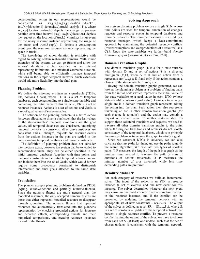
Temporal DatabasesOur approach is similar to chronicles in the IxTeT system (M. Ghallab, 1994). For each state variable we use a single temporal database that consists of a partially ordered sequence of changes and requests, where a changerepresents the change of the state variable’s value and the request represents a request on the state variable to keep certain value for a period of time.

Formally, for a state-variable with domain D, change is a quadruple (xs,xe,vinitial,vfinal), where xs, xe are time points, vinitial, vfinal D, and request is a triple (xs,xe,v), where xs, xe are time points and v D. We say that the temporal database is consistent, if any two consecutive changes share the inner value and any request between those two changes shares their inner value as well.

The partial ordering of the changes and requests consists of total ordering of the changes, which is constructed as a result of strong decisions of the search algorithm, and partially ordered requests. Figure 1 illustrates an example of the temporal database.

Figure 1. Illustration contains two changes (1two requests on the value 2. Time points are represented as letters a-h. The labels of arcs represent constraints from the underlying temporal network (e.g. b happens at least 2 and at most units before e), which also determine the total ordering of the changes. The temporal relations between requests are unimportant with regard to the temporal database.

Single temporal database for a state variable can be conceptually seen as a timeline, a structure known in context of planners RAX-PS (Jonsson, Morris, Muscettola, Rajan, & Smith, 2000) and EUROPA (Frank & Jonsson, 2001), recently also forming a base of systems Timeline-based Representation Framework (Cesta & Fratini, 2008)and Constraint Network on Timelines (Verfaillie & Prelet, 2008). In terms of our temporal databases, timelines contain solely the requests on values, while the function of changes is provided by various approaches, often formulated as a CSP. By totally ordering the changes in the databases we sacrifice some flexibility of the final plan in

favour of the planning system performance; the ordering of the changes is what makes our temporal databases different from recent partial order causal link planners such as VHPOP (Younes & Simmons, 2003)

ResourcesThough resources can be modelled via state-variables, we approach the modelling of resources separately by creating for each planning problem a set of resource instances, where each instance corresponds to a single resource appearing in the problem. By itself the resource instance is a set of resource events, which take different forms based on the type of resource the instance is representing. In Filuta we have modelled well known unary resources, discrete resources and reservoirs (Laborie, 2001).

Unary Resource corresponds to a single machine that can support only one activity at any given time. An instance of the unary resource is a set of resource events, where each event consists of a pair of time points that represent the start and the end of the event.

Discrete Resource corresponds to a pool of multiple uniform machines. An instance of the discrete resource is a set of resource events, where each event is defined as a triple (xs,xe,rq), where xs, xe are time points, and rq N represents the number of required machines. Each resource instance has a fixed capacity.

Reservoir is a resource that can be consumed and produced and consumption and production events may not happen in tandem. An instance of the reservoir resource is a set of events, where each event is defined as a pair (x,e), where x is a time point and e Z is a relative change of the resource level; e < 0 represents consumption and e > 0 represents production. Each instance has fixed capacity.

ActionsActions are grounded temporal operators that describe changes of the state-variables’ values, requests on valuesof the state-variables, and resource events on the resource instances. Each action includes temporal parameters representing the start and the end of the action; action instances are derived from actions by instantiating their temporal parameters allowing multiple instances of a single action in the plan.

Formally, action is a sextuple (tps, tpe, dur, CHs, RQs, REs), where tps and tpe are time point parameters, dur N is a duration of the action, CHs is a set of changes of the state-variables, RQs is a set of requests on the state-variables, and REs is a set of resource events (consumption/production) upon the resource instances.

For example we can imagine an action load-truck3-package2-location1 that represents loading the package2 into the truck3 at the location1. The action takes 5 time units to execute, the truck has a limited capacity, loading a package requires a crane and the package2 requires 11 units of space. We further assume we have state-variable svp and svt, where svp represents the position of the package2 and svt represents the location of the truck3. The


6

corresponding action in our representation would be constructed as (x,y,5,{svp[x,y]:location1{svt -cap[y]:-svp[x,y]:location1position over time interval [x,y], svt[x,y]:location1 depicts the request on the location of truck3, crane[x,y] is an event for the unary resource instance representing the usage of the crane, and truck3-cap[y]:-11 depicts a consumption event upon the reservoir resource instance representing the space in truck3.

The knowledge of action duration is restrictive with regard to solving certain real-world domains. With minor extension of the system, we can go further and allow the actions’ durations to be specified as an interval representing its minimal and maximal estimated duration, while still being able to efficiently manage temporal relations in the simple temporal network. Such extension would add more flexibility into the final plan.

Planning ProblemWe define the planning problem as a quadruple (TDBs, RIs, Actions, Goals), where TDBs is a set of temporal databases, each corresponding to a single state-variable and containing the initial value of this variable, RIs is a set of resource instances, Actions is a set of actions and Goals is a set of goal values of state-variables.

The solution of the planning problem is a set of action instances allocated to time (a plan) such that the last values of the state-variables’ temporal evolutions are the goal values, all temporal databases are consistent, underlying temporal network is consistent, all resource instances are consistent, and all changes, requests and resource events from the actions instances in the plan are settled in the corresponding temporal databases and resource instances.

The definition of planning problem does not consider intermediate goals; however the system can be extended to accommodate them. They can be either specified in the initial temporal databases (together with time points and temporal constraints in the initial temporal network), or we can include them into the set of Goals, which would further require some precedence constraint to distinguish intermediate and final goals attached to the same state variables.

TranslationThe planner accepts planning problems defined in PDDL (typing, durative-actions and partially numeric-fluents). Since the numeric fluents are more general than the modelled resources, the only accepted numeric fluents are those that either represent modelled resource or disappear through grounding. The numeric fluents that represent resources are automatically translated into the planner's representation by checking grounded actions for increase and decrease effects, corresponding fluents and their numerical comparisons, and creating resource instances instead of the fluents.

Solving ApproachFor a given planning problem we use a single STN, whose time points are used for temporal annotation of changes, requests and resource events in temporal databases and resource instances. The resource reasoning is realized by a resource manager, which keeps a least-commitment approach by maintaining the potential resource conflicts (overconsumptions and overproductions of a resource) as a CSP. Upon the state-variables we further build domain transition graphs (Jonsson & Bäckström, 1998).

Domain Transition GraphsThe domain transition graph (DTG) for a state-variable with domain D and a set of actions S is a directed multigraph (V,E), where V = D and an action from S represents arc (vi,vj) E if and only if the action contains a change of the state-variable from vi to vj.

Having the domain transition graphs generated, we can look at the planning problem as a problem of finding paths from the initial node (which represents the initial value of the state-variable) to a goal value in each DTG (whose state-variable contains a goal value). However traversing a single arc in a domain transition graph represents adding the action into the plan. Such action then also represents traversing an arc in other domain transition graphs (for each change it contains), and the action may contain a request on certain value of another state-variable. To support these collateral transitions and requests, we need to traverse all other domain transition graphs to the point when the original transitions and requests do not violate consistency of the temporal databases, which is in principle the same problem as traversing the graph to satisfy a goal.

Since we construct DTGs in advance, we can also calculate shortest paths for them, and use the paths to guide the search algorithm. We calculate two types of shortest paths. T-P measures the length of the path in a graph as the minimal time needed to traverse the path (a sum of durations of actions traversed). OT-P measures the minimal number of arcs traversed, while less time demanding paths are preferred.

Resource ManagerFor each category of resources we built an incremental solver. The input of the solver is an STN, a resource instance (a set of events), and one new event for this instance. The solver determines whatever the new event may cause an overproduction or overconsumption conflict in the resource instance, and if the conflict can be prevented by updating the temporal network with an appropriate set of new constraints – resolvers. The output of the solver is defined as a set SR = {S1,…,Sn iis a set of resolvers – updates of the temporal network that prevent a single resource conflict. To prevent a resource conflict having the output of the solver, we have to choose from each set Si (at least) one update, such that the set of chosen updates is consistent with the temporal network.


7

Trivial cases occur when SR = , which indicates that no conflicts need to be resolved, and SR, indicating that some resource conflict cannot be resolved.

Planning problems generally contain multiple resource instances and the solvers together often produce multiple sets SR1, …, SRn. The formulation of the solvers output now becomes helpful as we can aggregate the outputs into one set SR = SR1 … SRn. The purpose of the resource manager is to maintain the aggregated set SR of resolvers. The maintenance consists of removing updates inconsistent with given STN and checking the existence of solution (a selection of an update from each element of SR). Given an STN, to find a solution for SR we run a depth-first search in the space of possible choices of updates, while each choice is followed by realizing the update operation upon the STN and consequent removal of inconsistent updates. To improve efficiency, the resource manager works only with a sub-network of the STN (taking only the time points contained in the updates in SR).

In other words, the resource manager checks the existence of solution for a Disjunctive Temporal Problem (Stergiou & Koubarakis, 1998), which is incrementally built from the sub-network of the current STN and disjunctive constraints imposed by the resource-specific solvers.

We can see the resource manager as a coordinator of multiple resource-specific incremental solvers that are invoked only when a new resource event is introduced by an action, in which case the concerned solver produces a set of sets of temporal constraints, which are from that point on handled solely by the resource manager as a DTP.

The architecture of the resource manager is highly extensible; other resource models can be “plugged in” to support different types of resources. Current resource models include solvers for unary resources, discrete resources and two types of reservoirs (one supports only relative consumption/production events, the second one supports asymmetric events – e.g. resource is consumed relatively and produced absolutely, we can imagine an example of such resource as the fuel in a car that is consumed by driving the car (relative consumption) and the car is always refuelled to maximum capacity (absolute production).

Search AlgorithmIn the Filuta system we adapted the plan-space planning approach (Ghallab, Nau, & Traverso, 2004), where the search space consists of states representing partially specified plans (note that the search state differs from the world state). For a planning problem (TDBs, RIs, Actions, Goals) we define the initial state as a quintuple s0 = (STN, TDBs’, RIs’, SR, Plan), where TDBs’ = TDBs, RIs’ = RIs, SR = , Plan = and STN is the initial temporal network.

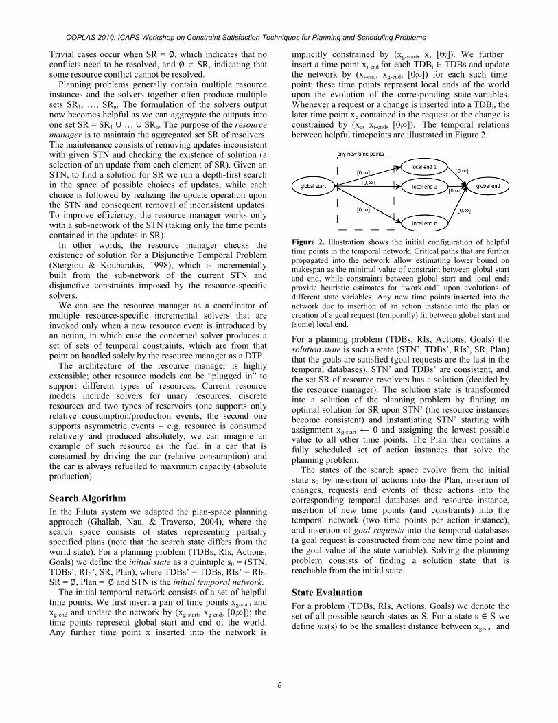
The initial temporal network consists of a set of helpful time points. We first insert a pair of time points xg-start and xg-end and update the network by (xg-start, xg-end, [0,time points represent global start and end of the world. Any further time point x inserted into the network is

implicitly constrained by (xg-start, x, [0,insert a time point xi-end for each TDBi TDBs and update the network by (xi-end, xg-end, [0,point; these time points represent local ends of the world upon the evolution of the corresponding state-variables. Whenever a request or a change is inserted into a TDBi, the later time point xe contained in the request or the change is constrained by (xe, xi-end, [0, The temporal relations between helpful timepoints are illustrated in Figure 2.

Figure 2. Illustration shows the initial configuration of helpful time points in the temporal network. Critical paths that are further propagated into the network allow estimating lower bound on makespan as the minimal value of constraint between global start and end, while constraints between global start and local ends provide heuristic estimates for “workload” upon evolutions of different state variables. Any new time points inserted into the network due to insertion of an action instance into the plan or creation of a goal request (temporally) fit between global start and (some) local end.

For a planning problem (TDBs, RIs, Actions, Goals) the solution state is such a state (STN’, TDBs’, RIs’, SR, Plan)that the goals are satisfied (goal requests are the last in the temporal databases), STN’ and TDBs’ are consistent, and the set SR of resource resolvers has a solution (decided by the resource manager). The solution state is transformed into a solution of the planning problem by finding an optimal solution for SR upon STN’ (the resource instances become consistent) and instantiating STN’ starting with assignment xg-start 0 and assigning the lowest possible value to all other time points. The Plan then contains a fully scheduled set of action instances that solve the planning problem.

The states of the search space evolve from the initial state s0 by insertion of actions into the Plan, insertion of changes, requests and events of these actions into the corresponding temporal databases and resource instance, insertion of new time points (and constraints) into the temporal network (two time points per action instance), and insertion of goal requests into the temporal databases (a goal request is constructed from one new time point and the goal value of the state-variable). Solving the planning problem consists of finding a solution state that is reachable from the initial state.

State EvaluationFor a problem (TDBs, RIs, Actions, Goals) we denote the set of all possible search states as S. For a state s S we define ms(s) to be the smallest distance between xg-start and


8

xg-end in the corresponding STN (the lower bound for makespan), and ft(s) to be the sum of smallest distances between xg-start and xi-end for all end points in TDBs (the lower bound for the sum of times to achieve all last values in TDBs).

We define the state evaluation function eval: S as eval(s) = (ms(s), ft(s)) and the goal of planner is to find a reachable solution state with the lexicographically minimal value of the eval function.

The state evaluation reflects simple empirical heuristic that it is better to choose less time demanding actions even if in the current context the estimate for makespan does not change; additionally the ft estimate supports “load balancing” among time requirements of the state variables’ evolutions.

Search ProceduresThe search algorithm divides into four interleaved search procedures root_search, way_search, support_search and resource_search. The input of all procedures is a state and the current upper bound, which can be an evaluation of the best state found so far, it can be given arbitrarily (makespan of the previous random restart), or it can be unknown (represented as ( , )). The output of the procedures is a state, where a state = indicates that either all states in sub-tree were pruned (the lower bound exceeded the upper bound), or the sub-tree does not contain the intended partial solution. The interaction between search procedures is depicted in Figure 4.

For a problem (TDBs, RIs, Actions, Goals), the root_search (Algorithm 1) proceeds by picking a goal value of a state-variable from Goals that is not currently achieved (the last change in the corresponding TDB does not support the goal value), building a goal request (from a new time point in STN and the goal value) and calling the way_search to find a way in the corresponding DTG to support the goal requests (lines 05-09). The process is iterated until a solution state is found; the solution state is constructed incrementally as the first call of the way_search takes the initial state s0 and returns state s1, which is taken by the consecutive call of the way_searchand so on (a goal request can be constructed multiple times for one goal value as way_search may invalidate a previously achieved goal). This is similar to STRIPS algorithm for classical planning.

The way_search (Algorithm 1) deals with the problem of finding a way in a domain transition graph from an anchoring change (for the goal request the anchoring change is the last change in the corresponding TDB, otherwise the anchoring change is provided by support_search) to a given fact that is either a change or a request. The way_search initially imposes new constraints into the current STN to improve the lower bound according to eval; the constraints represent the minimal time needed to traverse the path in DTG from the final value of the anchoring change to the initial value of the fact (we use the value of the shortest path T-P). To find the best path in the DTG (according to eval) way_search recursively performs

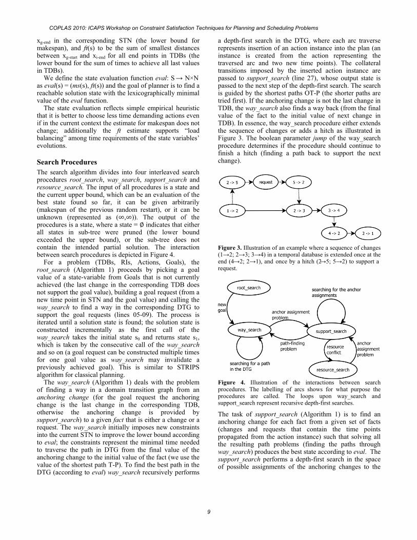
a depth-first search in the DTG, where each arc traverse represents insertion of an action instance into the plan (an instance is created from the action representing the traversed arc and two new time points). The collateral transitions imposed by the inserted action instance are passed to support_search (line 27), whose output state is passed to the next step of the depth-first search. The search is guided by the shortest paths OT-P (the shorter paths are tried first). If the anchoring change is not the last change in TDB, the way_search also finds a way back (from the final value of the fact to the initial value of next change in TDB). In essence, the way_search procedure either extends the sequence of changes or adds a hitch as illustrated in Figure 3. The boolean parameter jump of the way_search procedure determines if the procedure should continue to finish a hitch (finding a path back to support the next change).

Figure 3. Illustration of an example where a sequence of changes (1end (4 once by a hitch (2request.

Figure 4. Illustration of the interactions between search procedures. The labelling of arcs shows for what purpose the procedures are called. The loops upon way_search and support_search represent recursive depth-first searches.

The task of support_search (Algorithm 1) is to find an anchoring change for each fact from a given set of facts (changes and requests that contain the time points propagated from the action instance) such that solving all the resulting path problems (finding the paths through way_search) produces the best state according to eval. The support_search performs a depth-first search in the space of possible assignments of the anchoring changes to the


9

facts. The search is guided by the fewest-options-firstprinciple.

Algorithm 1. Search procedures root_search, way_search and support_search.

01 root_search02 open_goals goals

(s0, goals, bound)

03 s 004 while open_goals 05 foreach goal open_goals06 tp new time point in s.stn07 change the latest change in s.TDB08 request (goal, tp)09 s way_search(s, change, request, bound, false)10 if s = return11 update open_goals with s12 return s1314 way_search15 if eval(s) > bound return

(s, ch, fact, bound, jump)

16 if ch.vfinal = fact.vinitial17 if jump18 ch’ 19 s way_search(s, fact, ch’, bound, false)20 return s21 my_best 22 foreach a aplicable_actions23 bound 24 ai a25 s.Plan {ai26 facts ai27 found support_search(s,facts,bound)28 if found29 ch’ nd.TDB added by ai30 found31 if found my_best 32 return my_best3334 support_search35 if eval(s) > bound return

(s, facts, bound)

36 my_best 37 choose f facts38 foreach ch suitable changes for fact39 bound40 if ch is the last in s.TDB41 found ch, f,bound,false)42 else43 found ch,f,bound,true)44 if found 45 found \{f46 if found my_best 47 return my_best

The resource_search procedure (Algorithm 2) is called whenever the set SR in the current state becomes inconsistent (the consistency check fails); this occurs mainly upon the insertion of a resource event into a resource instance. The resource_search identifies the inconsistent resource instance and systematically tries to extend the plan by an action that contains a helpful event for the inconsistent resource instance and the choice of the action is the best according to eval; for example the helpful

event can be a production event for a reservoir instance, which was over consumed. Same as in way_search, the facts (changes and requests in the chosen action) are passed to support_search.

In essence, the search procedures branch on choices of actions in domain transition graphs (way_search), choices of temporal context of facts (anchor assignments in support_search) and choices of actions to resolve a resource conflict (resource_search), while the lower bound is carried in the simple temporal network (the lower bound comes from the propagation of critical paths T-P into the network). Then for each open goal, the algorithm tries to find combination of action instances and ordering constrains such that merging them with the current partial plan (rather than adding them to the end of plan) produces another partial plan that satisfies the goal and is the best according to the state evaluation.

Although the procedures way_search, support_search and resource_search perform complete depth-first searches, they are in global sense greedy as each of them considers only the locally optimal results of the other two.

Random RestartsThe described search algorithm assumes a given ordering of the goal values in the planning problem. We further extended the algorithm with random restarts (Algorithm 2)of the ordering of the goal values (we explore random permutations of the sequence of the goal values). The random restarts are helpful for tightening the upper bound for consecutive searches, which significantly improves pruning the search space. This is the same technique as used in Anytime Weighted A* introduced in (Hansen & Zhou, 2007).

Algorithm 2. Search procedures resource_search and RR (random restarts).

01 resource_search02 AR

(s, bound)

03 my_best 04 foreach a AR05 bound 06 facts ai07 ai a08 s.Plan {ai09 facts ai10 found support_search(s,facts,bound)11 if found my_best 12 return my_best1314 RR15 best

(s0, goals)

16 while not stopped17 s 018 next_perm e_randomly(goals)19 s20 s21 if s best


10

A reason for using a simple depth-first search inway_search and support_search procedures (as opposed to A*) is based on the considerable memory requirements of the simple temporal network, which is a part of each search state and grows in O(n2), where n is the number of time points; the growth of the temporal network would directly impact the number of states that could be queued deeper in the search tree.

Further discussion of the algorithm can be found in.

Experimental ResultsWe implemented the Filuta system in Java and compared it with the best planners competing in the latest planning competition. In particular, to evaluate the efficiency of resource reasoning integration into planning we used three temporal planning domains with significant presence of resource reasoning: Openstacks, Elevators, and Transport from the deterministic temporal satisficing track of IPC 2008 (Helmert, Do, & Refanidis, 2008) and compared planning systems competing in this track, namely SGPlan6 (the winner), TFD (the runner-up), and Base-line planner proposed by the competition organizers.

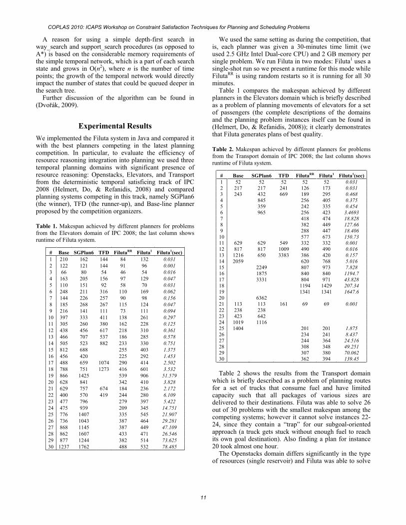
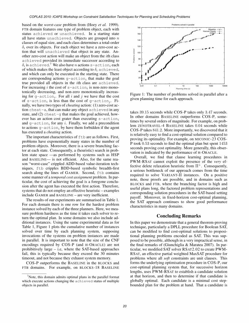
Table 1. Makespan achieved by different planners for problems from the Elevators domain of IPC 2008; the last column shows runtime of Filuta system.

# SGPlan6 TFD FilutaRR Filuta1 Filuta1(sec)1 210 162 144 84 132 0.0312 122 121 144 91 96 0.0013 66 80 54 46 54 0.0164 163 205 156 97 129 0.0475 110 151 92 58 70 0.0316 248 211 316 110 169 0.0627 144 226 257 90 98 0.1568 185 268 267 115 124 0.0479 216 141 111 73 111 0.09410 397 333 411 138 261 0.29711 305 260 380 162 228 0.12512 438 456 617 218 310 0.36113 466 707 537 186 285 0.57814 505 523 882 233 330 0.75115 812 688 255 403 1.37516 456 420 225 292 1.45317 488 659 1074 290 414 2.50218 788 751 1273 416 601 3.53219 866 1425 539 906 51.57920 628 841 342 410 3.82821 629 757 674 184 236 2.17222 400 570 419 244 280 6.10923 477 796 279 397 5.42224 475 939 209 345 14.75125 776 1407 335 545 21.90726 736 1043 387 464 29.28127 868 1145 387 449 47.10928 862 1607 433 471 26.54629 877 1244 382 514 73.62530 1237 1762 488 532 78.485

We used the same setting as during the competition, that is, each planner was given a 30-minutes time limit (we used 2.5 GHz Intel Dual-core CPU) and 2 GB memory per single problem. We run Filuta in two modes: Filuta1 uses a single-shot run so we present a runtime for this mode while FilutaRR is using random restarts so it is running for all 30 minutes.

Table 1 compares the makespan achieved by different planners in the Elevators domain which is briefly described as a problem of planning movements of elevators for a set of passengers (the complete descriptions of the domains and the planning problem instances itself can be found in (Helmert, Do, & Refanidis, 2008)); it clearly demonstrates that Filuta generates plans of best quality.

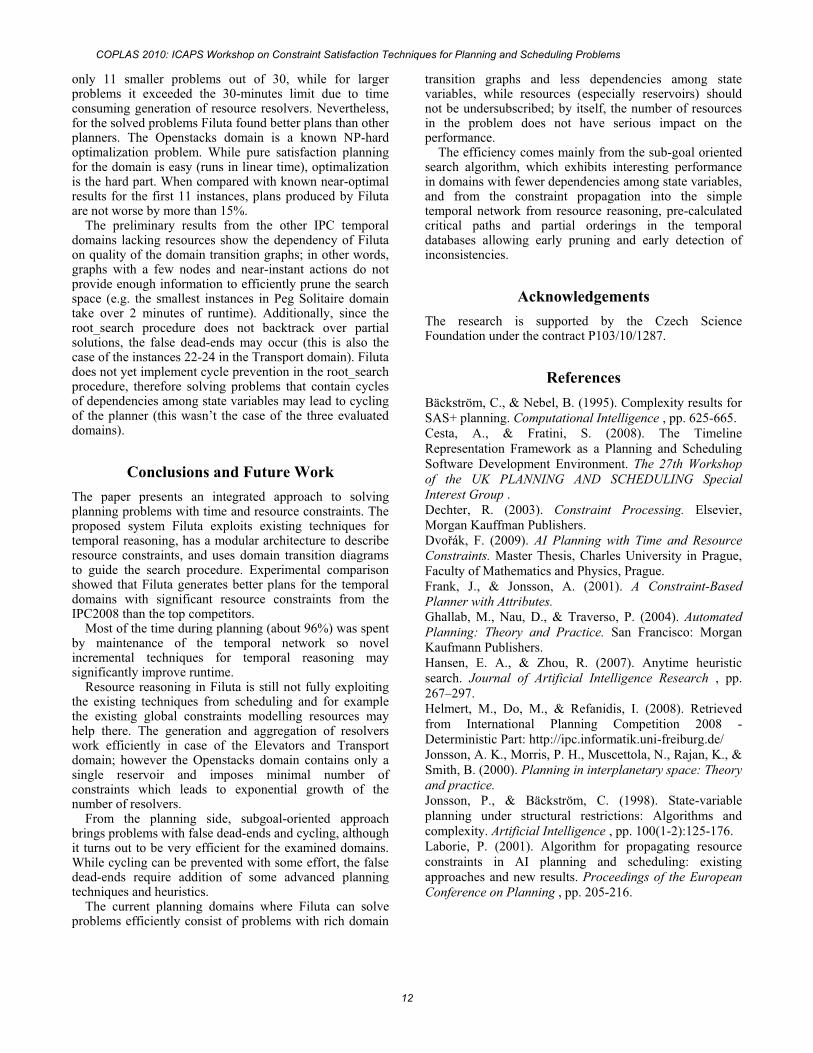
Table 2. Makespan achieved by different planners for problems from the Transport domain of IPC 2008; the last column shows runtime of Filuta system.

# SGPlan6 TFD FilutaRR Filuta1 Filuta1(sec)1 52 52 52 52 52 0.0312 217 217 241 126 173 0.0313 243 432 669 189 295 0.4684 845 256 405 0.3755 359 242 335 0.4546 965 256 423 3.46937 418 474 18.8288 382 449 127.669 288 447 18.40610 577 673 150.7311 629 629 549 332 332 0.00112 817 817 1009 490 490 0.01613 1216 650 3383 386 420 0.15714 2059 620 768 5.01615 2249 807 973 7.82816 1875 840 840 1194.717 3331 804 971 43.82818 1194 1429 207.3419 1341 1341 1647.620 636221 113 113 161 69 69 0.00122 238 23823 423 64224 1019 111625 1404 201 201 1.87526 234 241 8.43727 244 364 24.51628 308 348 49.25129 307 380 70.06230 362 394 139.45

Table 2 shows the results from the Transport domain which is briefly described as a problem of planning routes for a set of trucks that consume fuel and have limited capacity such that all packages of various sizes are delivered to their destinations. Filuta was able to solve 26 out of 30 problems with the smallest makespan among the competing systems; however it cannot solve instances 22-24, since they contain a “trap” for our subgoal-oriented approach (a truck gets stuck without enough fuel to reach its own goal destination). Also finding a plan for instance 20 took almost one hour.

The Openstacks domain differs significantly in the type of resources (single reservoir) and Filuta was able to solve


11

only 11 smaller problems out of 30, while for larger problems it exceeded the 30-minutes limit due to time consuming generation of resource resolvers. Nevertheless, for the solved problems Filuta found better plans than other planners. The Openstacks domain is a known NP-hard optimalization problem. While pure satisfaction planning for the domain is easy (runs in linear time), optimalization is the hard part. When compared with known near-optimal results for the first 11 instances, plans produced by Filuta are not worse by more than 15%.

The preliminary results from the other IPC temporal domains lacking resources show the dependency of Filuta on quality of the domain transition graphs; in other words, graphs with a few nodes and near-instant actions do not provide enough information to efficiently prune the search space (e.g. the smallest instances in Peg Solitaire domain take over 2 minutes of runtime). Additionally, since the root_search procedure does not backtrack over partial solutions, the false dead-ends may occur (this is also the case of the instances 22-24 in the Transport domain). Filuta does not yet implement cycle prevention in the root_search procedure, therefore solving problems that contain cycles of dependencies among state variables may lead to cycling of the planner (this wasn’t the case of the three evaluated domains).

Conclusions and Future WThe paper presents an integrated approach to solving planning problems with time and resource constraints. The proposed system Filuta exploits existing techniques for temporal reasoning, has a modular architecture to describe resource constraints, and uses domain transition diagrams to guide the search procedure. Experimental comparison showed that Filuta generates better plans for the temporal domains with significant resource constraints from the IPC2008 than the top competitors.

Most of the time during planning (about 96%) was spent by maintenance of the temporal network so novel incremental techniques for temporal reasoning may significantly improve runtime.

Resource reasoning in Filuta is still not fully exploiting the existing techniques from scheduling and for example the existing global constraints modelling resources may help there. The generation and aggregation of resolvers work efficiently in case of the Elevators and Transport domain; however the Openstacks domain contains only a single reservoir and imposes minimal number of constraints which leads to exponential growth of the number of resolvers.

From the planning side, subgoal-oriented approach brings problems with false dead-ends and cycling, although it turns out to be very efficient for the examined domains. While cycling can be prevented with some effort, the false dead-ends require addition of some advanced planning techniques and heuristics.

The current planning domains where Filuta can solve problems efficiently consist of problems with rich domain

transition graphs and less dependencies among state variables, while resources (especially reservoirs) should not be undersubscribed; by itself, the number of resources in the problem does not have serious impact on the performance.

The efficiency comes mainly from the sub-goal oriented search algorithm, which exhibits interesting performance in domains with fewer dependencies among state variables, and from the constraint propagation into the simple temporal network from resource reasoning, pre-calculated critical paths and partial orderings in the temporal databases allowing early pruning and early detection of inconsistencies.

The research is supported by the Czech Science Foundation under the contract P103/10/1287.

ReferencesBäckström, C., & Nebel, B. (1995). Complexity results for SAS+ planning. Computational Intelligence , pp. 625-665.Cesta, A., & Fratini, S. (2008). The Timeline Representation Framework as a Planning and Scheduling Software Development Environment. The 27th Workshop of the UK PLANNING AND SCHEDULING Special Interest Group .Dechter, R. (2003). Constraint Processing. Elsevier, Morgan Kauffman Publishers.

AI Planning with Time and Resource Constraints. Master Thesis, Charles University in Prague, Faculty of Mathematics and Physics, Prague.Frank, J., & Jonsson, A. (2001). A Constraint-Based Planner with Attributes.Ghallab, M., Nau, D., & Traverso, P. (2004). Automated Planning: Theory and Practice. San Francisco: Morgan Kaufmann Publishers.Hansen, E. A., & Zhou, R. (2007). Anytime heuristic search. Journal of Artificial Intelligence Research , pp. 267–297.Helmert, M., Do, M., & Refanidis, I. (2008). Retrieved from International Planning Competition 2008 -Deterministic Part: http://ipc.informatik.uni-freiburg.de/Jonsson, A. K., Morris, P. H., Muscettola, N., Rajan, K., & Smith, B. (2000). Planning in interplanetary space: Theory and practice.Jonsson, P., & Bäckström, C. (1998). State-variable planning under structural restrictions: Algorithms and complexity. Artificial Intelligence , pp. 100(1-2):125-176.Laborie, P. (2001). Algorithm for propagating resource constraints in AI planning and scheduling: existing approaches and new results. Proceedings of the European Conference on Planning , pp. 205-216.


12

M. Ghallab, H. L. (1994). Representation and control in IxTeT, a temporal planner. International Conference on AI Planning Systems, (pp. 61-67).Stergiou, K., & Koubarakis, M. (1998). Backtracking algorithms for disjunctions of temporal constraints. 15th National Conference on Artificial Intelligence, (pp. 248-253).Verfaillie, G., & Prelet, C. (2008). Using Contraint Network on Timelines to Model and Solve Planning and Scheduling Problems. International Conference on Automated Planning and Scheduling 2008 , p. 272.Younes, H. L., & Simmons, R. G. (2003). VHPOP: versatile heuristic partial order planner. Journal of Artificial Intelligence Research , pp. 405-430.


13

Cost-Optimal Planning using Weighted MaxSAT

Nathan Robinson†, Charles Gretton‡, Duc-Nghia Pham†, Abdul Sattar††ATOMIC Project, Queensland Research Lab, NICTA and

Institute for Integrated and Intelligent Systems, Griffith University, QLD, Australia{nathan.robinson,duc-nghia.pham,abdul.sattar}@nicta.com.au

‡ School of Computer Science, University of [email protected]

Abstract

We consider the problem of computing optimal plans forpropositional planning problems with action costs. In thespirit of leveraging advances in general-purpose automatedreasoning for that setting, we develop an approach that oper-ates by solving a sequence of partial weighted MaxSAT prob-lems, each of which corresponds to a step-bounded variantof the problem at hand. Our approach is the first SAT-basedsystem in which a proof of cost optimality is obtained using aMaxSAT procedure. It is also the first system of this kind toincorporate an admissible planning heuristic. We perform adetailed empirical evaluation of our work using benchmarksfrom a number of International Planning Competitions.

IntroductionRecently there have been significant advances in the direc-tion of optimal planning procedures that operate by makingmultiple queries to a decision procedure, usually a BooleanSAT procedure. For example, the work of (Hoffmann etal. 2007) answers a key challenge from (Kautz 2006) bydemonstrating how existing SAT-based planning techniquescan be made effective solution procedures for fixed-horizonplanning with metric resource constraints. In the same vein,Russell & Holden (2010) and Giunchiglia & Maratea (2007)develop optimal SAT-based procedures for net-benefit plan-ning in fixed-horizon problems. In this setting actions havecosts and goal utilities can be interdependent. Moreover,in the direction of improving the scalability and efficiencyof SAT-based approaches in step-optimal (and indeed fixed-horizon) planning, (Robinson et al. 2009) presents an en-coding of step-bounded planning problems that shows sig-nificant performance gains over previous results. Large per-formance gains have also been demonstrated where efficientand sophisticated query strategies are employed (Streeter &Smith 2007; Rintanen 2004). Summarising, in the settingsof step-optimal and fixed-horizon planning, recent workshave demonstrated that SAT-based techniques inspired bysystems like BLACKBOX (Kautz & Selman 1999) continueto dominate other approaches.

Considering the planning literature more generally, nu-merous distinct criteria for plan optimality have been pro-posed. These include: (1) Minimise makespan (a.k.a. step-optimality); The objective is to find a plan of minimal length.(2) Minimise plan cost; Each action has a numeric cost, a

plan’s cost is the sum of the costs of its constituent actions,and an optimal plan has minimal cost. (3) Maximise net-benefit; States (resp. actions) have rewards (resp. costs), andan optimal plan is a sequence of actions executable from thestarting state that induces a behaviour of maximal utility –These problems are sometimes called oversubscribed, andwere recently shown to be equivalent (using a compilation)to the cost-optimising setting (Keyder & Geffner 2009). Onekey observation to be made is that the above optimality cri-teria are often conflicting. For example, a plan with minimalmakespan is not guaranteed to be cost- or utility-optimal. In-deed, in the general case there is no link between the numberof plans steps (planning horizon) and plan quality.

Existing SAT-based planning procedures are limited tomakespan-optimal and fixed-horizon settings – i.e., eitherthe objective is to minimise the number of plan-steps, orvalid optimal solutions are constrained to be of, or less than,a fixed length. Thus, their usefulness is limited in practice.For example, optimal SAT-based planning procedures wereunable to participate at the International Planning Competi-tion (IPC) in 2008 due to the adoption of a single optimi-sation criteria (cost-optimality). This paper overcomes thisrestriction, developing COS-P, the fist sound and completecost-optimal planning procedure based solely on a BooleanSAT(isfiability) procedure. Thus, we open the door to lever-aging SAT technology in planning settings with arbitrary op-timisation criteria.

The remainder of this paper is organised as follows. Wefirst give an overview of optimal propositional planningwith action costs, delete relaxations of that problem, andthe partial weighted MaxSAT optimisation problem. Wethen describe our approach in detail, developing compila-tions to partial weighted MaxSAT of the fixed-horizon plan-ning problem, and of the fixed horizon problem with a re-laxed suffix. Following this we develop our novel MaxSATsolution procedure PWM-RSAT. We then consider workmost related to our approach and empirically evaluate ourapproach on planning benchmarks from a number of IPCs.Finally we make concluding remarks and propose some ofthe more interesting directions for future research.


14

Background and NotationsPropositional planning with action costsA propositional planning problem with costs is a 5-tupleΠ = 〈P,A, s0,G, C〉. Here, P is a set of propositions thatcharacterise problem states; A is the set of actions that caninduce state transitions; s0 ⊆ P is the starting state; AndG ⊆ P is the set of propositions that characterise the goal.The function C : A → �+

0 is a bounded cost function thatassigns a positive cost-value to each action. This value cor-responds to the cost of executing the action.

Each action a ∈ A is described in terms of its precondi-tions pre(a) ⊆ P , positive effects eff•(a) ⊆ P , and neg-ative effects eff◦(a) ⊆ P . An action a can be executed ata state s ⊆ P when pre(a) ⊆ s. We write A(s) for theset of actions that can be executed at state s – Formally,A(s) ≡ {a|a ∈ A, pre(a) ⊆ s}. When a ∈ A(s) is ex-ecuted at s the successive state is (s∪ eff•(a))\eff◦(a). Ac-tions cannot both add and delete the same proposition – i.e.,eff•(a) ∩ eff◦(a) ≡ ∅.1 A state s is a goal state iff G ⊆ s.

Usually any two actions a1, a2 ∈ A are permitted to beexecuted instantaneously in parallel at a state provided anyserial execution of the actions is valid and achieves an iden-tical outcome. When two actions cannot be executed in par-allel we say they conflict. Supposing non-conflicting actionscan be executed instantaneously in parallel, a plan π is a dis-crete sequence of time-indexed sets of non-conflicting ac-tions which, when applied to the start state, lead to a goalstate. We say a plan is serial (a.k.a. linear plan), denoted �π,if each time-indexed set contains one action. Finally, whereAi is the set of actions at step i of π = [A1,A2, ..,Ah], thecost of π, written C(π), is:

C(π) =h∑

i=1

∑

a∈Ai

C(a)

A number of different conditions for plan optimality canbe defined. In particular, a plan is parallel step-optimal if noshorter plan of the same parallel format exists. The defini-tion for serial step-optimality is identical, but also respectsthe condition that a valid plan has only one action executedat each step. A plan π∗ is cost-optimal if there is no plan πs.t. C(π) < C(π∗). Finally, we draw the reader’s attention tothe fact that the definition of cost optimality is not dependenton the plan format.

The relaxed planning problemA delete relaxation Π+ of a planning problem Π is an equiv-alent problem in all respects except the definition of actions.In particular, the set of actions A+ in Π+ comprises the el-ements a ∈ A from Π altered so that eff◦(a) ≡ ∅. The re-laxed problem has two key properties of interest here. First,the cost of an optimal plan from any reachable state in Πis greater than or equal to the cost of the optimal plan fromthat state in Π+. Consequently relaxed planning can yield auseful admissible heuristic in search. For example, a best-first search such as A∗ can be heuristically directed towards

1In practice this case is given a special semantics, the details ofwhich shall not be considered further here.

an optimal solution by using the costs of relaxed plans to ar-range the priority queue. Second, although NP-hard to solveoptimally in general (Bylander 1994), in practice optimal so-lutions to the relaxed problem Π+ are more easily computedthan for Π.

Partial weighted MaxSATA Boolean SAT problem is a decision problem, instances ofwhich are typically expressed as a CNF propositional for-mula. A CNF corresponds to a conjunction over clauses,each of which corresponds to a disjunction over literals. Aliteral is either a proposition (i.e., Boolean variable symbol)or its negation. Where |= denotes semantic entailment forpropositional logic, a solution associated with a formula φ isan assignment (a.k.a. valuation) V of truth values to propo-sitions with the property V |= φ.

A Boolean MaxSAT problem is an optimisation problemrelated to SAT. In practice a problem instance is again typ-ically expressed as a CNF, however the objective now is tocompute a valuation that maximises the number of satisfiedclauses. In detail, writing κ ∈ φ if κ is a clause in formulaφ, and taking V |= κ to have numeric value 1 when valid,and 0 otherwise, a solution V∗ to a MaxSAT problem has theproperty:

V∗ = arg maxV

∑

κ∈φ(V |= κ) (1)

A weighted MaxSAT problem (Josep Argelic and, Manya,& Planes 2008), denoted ψ, is a MaxSAT problem whereeach clause κ ∈ ψ has a bounded positive numerical weightω(κ). The optimal solution V∗ to a ψ satisfies the followingequation:

V∗ = arg maxV

∑

κ∈ψω(κ)(V |= κ) (2)

Finally, the partial weighted MaxSAT problem (Fu & Ma-lik 2006) is a variant of weighted MaxSAT that distinguishesbetween hard and soft clauses. Only soft clauses are givena weight. In these problems a solution is valid iff it satisfiesall hard clauses. Therefore we have a notion of satisfiabil-ity. In particular, if the hard problem fragment of a partialweighted MaxSAT formula is unsatisfiable, then we say theformula is unsatisfiable. The definition of satisfiable followsnaturally. An optimal solution to a partial weighted MaxSATproblem is an assignment V∗ that is both valid and satisfiesEquation 2.

COS-PWe now describe COS-P, our planner that operates by iter-atively solving variants of n-step-bounded instances of theproblem at hand for successively larger n. Solutions to theintermediate step-bounded instances are obtained by com-piling them into equivalent partial weighted MaxSAT prob-lems, and then using our own MaxSAT procedure PWM-RSAT to compute their optimal solutions.

COS-P compiles and solves two variants, VARIANT-Iand VARIANT-II, of the intermediate instances. Those are


15

characterised in terms of their optimal solutions. Adopt-ing the notation Πn for the n-step-bounded variant of Π,VARIANT-I admits optimal solutions that correspond to min-imal cost plans for Πn. VARIANT-II admits optimal planswith the following structure. Each has a prefix which cor-responds to n sets of actions from Πn.2 Plans can have anarbitrary length suffix (including length 0) comprised of ac-tions from the delete relaxation Π+.

Both variants can be categorised as direct, constructive,and tightly sound. They are direct because we have aBoolean variable in the MaxSAT problem for every actionand state proposition at each plan step. They are constructivebecause any satisfying model and its cost in the MaxSAT in-stances corresponds to a plan and its cost in the source prob-lem. Critically, our compilations are tightly sound, in thesense that every plan with cost c in the source planning prob-lem has a corresponding satisfying model of cost c in theMaxSAT encoding and vice versa. This permits two key ob-servations about VARIANT-I and VARIANT-II. First, whenboth variants yield an optimal solution, and both those solu-tions have identical cost, then the solution to VARIANT-I isa cost-optimal plan for Π. Second, if Π is soluble, then thereexists some n for which the observation of global optimalityshall be made by COS-P. Finally, we have that COS-P is asound and complete optimal planning procedure for propo-sitional problems with action costs.

For the remainder of this section we give the compilationfor VARIANT-I and VARIANT-II. In the following sectionwe describe the MaxSAT procedure PWM-RSAT that wedeveloped for use by COS-P.

Variant-I: bounded cost-optimal planningWe now describe a direct compilation of the bounded propo-sitional planning problem with action costs to a partialweighted MaxSAT formula ψ. The source of our compi-lation is the plangraph. This is an obvious choice becausereachability and neededness analysis performed during con-struction of the plangraph yield important mutex constraintsbetween action and propositional variables (Blum & Furst1997). Such constraints are not deduced independentlyby modern SAT procedures such as RSAT2.02 (Rintanen2008).

Below, we develop our compilation in terms of a listof 8 axiom Schemata. Whereas the standard definition ofweighted MaxSAT imposes the restriction that weights arepositive, we find it convenient for the remainder of our paperto admit negative weights. The first 7 capture the hard log-ical planning constraints, and Schema 8 reflects the actioncosts. Overall, the schemata we develop below make use ofthe following propositional variables. For each action occur-ring at a step t = 0, .., n − 1 (excluding noop actions), wehave a variable at. We define a fluent to be a state proposi-tion whose truth value can be modified by action executions.For each fluent occurring at step t = 0, .., n we have a vari-able pt. Also, we have make(p) ≡ {a|a ∈ A, p ∈ eff•(a)},and break(p) ≡ {a|a ∈ A, p ∈ eff◦(a)}. Lastly, below we

2i.e., an n-step plan prefix in the parallel format.

avoid annotating variables with their time index if it is clearfrom the context.

1. Start state axioms (hard): A unit clause containing p0

for every p ∈ s0.2. Goal axioms (hard): A unit clause containing pn for

every p ∈ G.3. Precondition and effect axioms (hard): For every ac-

tion a at each plan step t, we have clauses that require: (1)The action implies its precondition, (2) The action impliesits positive effects, and (3) The action implies its negativeeffects.

at → ∧p∈pre(a) p

t ∧at → ∧

p∈eff•(a) pt+1 ∧

at → ∧p∈eff◦(a) ¬pt+1

4. Propositional mutex axioms (hard): For every pair ofmutex fluents p1 and p2 at step t, we have a clause:

¬pt1 ∧ ¬pt25. Action mutex axioms (hard): For every pair of mutex

actions a1 and a2 at step t, we have a clause:

¬at1 ∧ ¬at26. At least one action axioms (hard): Where At is the set

of actions at step t, we have a clause that requires at leastone action be executed at step t:

∨

at∈At

at

7. Frame axioms (hard): These constrain how the truthvalues of fluents change over successive plan steps. For eachproposition pt, t > 0 we include the following clauses:

pt → (pt−1 ∨∨

a∈make(p)at−1)

¬pt → (¬pt−1 ∨∨

a∈break(p)at−1)

8. Action cost axioms (soft): Finally, we have a set of softconstraints for actions. In particular, for each action variableat such that C(a) > 0, we have a unit clause κi := {¬at}and have ω(κi) = −C(a).

Variant-II: n-step with a relaxed suffixWe describe a direct compilation of the problem Πn fromthe previous section, along with the addition of a causal en-coding of the delete relaxation, that we make available fromstep n.3 From hereon we refer to the latter as the relaxedsuffix.

Our encoding of the relaxed suffix is causal in the sensedeveloped in (Kautz, McAllester, & Selman 1996) for theirground parallel causal encoding of propositional planning inSAT. This requires additional variables to those developedfor VARIANT-I. In particular, for each fluent p and relaxedaction a ∈ A+ we have corresponding variables p+ and

3In VARIANT-II constraints from axiom 2 (goal axioms) areomitted from Πn.


16

a+. That p+i is true intuitively means: (1) That pni was false

(see VARIANT-I), and (2) That pi ∈ G, or p+i is the cause

of another fluent p+j in a relaxed suffix to the goal. That

a+ is true means that a is executed in the relaxed suffix.We also require a set of causal link variables. These arebest introduced in terms of a recursively defined set S∞ asfollows. For the base we take:

S0 ≡ {K(pi, pj)|a ∈ A+, pi ∈ pre(a), pj ∈ eff•(ai)}and then make the definition:

Si+1 ≡ Si ∪ {K(pj , pl)|K(pj , pk),K(pk, pl) ∈ Si}For each K(pi, pj) ∈ S∞ we have a corresponding variable.Intuitively, if K(pi, pj) is true then we say that pi is the causeof pj in the plan suffix.

VARIANT-II includes all schemata from VARIANT-I ex-cept the goal axioms of Schema 2. In addition, VARIANT-IIuses the following Schemata.

9. Relaxed goal axioms (hard): For each fluent p ∈ Gwe assert that it is either achieved at the planning horizon n,or using a relaxed action in A+. This is expressed with aclause:

pn ∨ p+

10. Relaxed fluent support axioms (hard): For each fluentp we have a clause:

p+ → (∨

a∈make(p)a+)

11. Causal link axioms (hard): For all fluents pi, takingall a ∈ make(pi) and pj ∈ PRE(a), we have the followingclause:

(p+i ∧ a+) → (pnj ∨ K(p+

j , p+i ))

This constraint asserts that if action a+1 is executed, then its

preconditions must be true at horizon n, or be supported bysome other action a+

2 with p2 ∈ eff•(a2).12. Causality implies cause and effect axiom (hard): For

each causal link variable K(p+1 , p

+2 ) we have a clause:

K(p+1 , p

+2 ) → (p+

1 ∧ p+2 )

13. Causal transitive closure axioms (hard): For each pairof causal link variables K(p+

1 , p+2 ) and K(p+

2 , p+3 ) we have

a clause:

(K(p+1 , p

+2 ) ∧ K(p+

2 , p+3 )) → K(p+

1 , p+3 )

14. Causal anti-reflexive axioms (hard): We assert thatfor a valid relaxed plan, the causal relation between fluentsmust exhibit irreflexivity. Hence, for each K(p+, p+) ∈ S∞we have a unit clause:

¬K(p+, p+)

Intuitively, this clause asserts that a fluent in the re-laxed suffix cannot support itself. For example, ina simple logistics example the fluent at(p, l)+ can be

achieved by a pair of relaxed actions, Pickup+ andDrop+, regardless of the location of package p. In thiscase, we have K(in-truck(t, p)+, at(p, l)+) via the action

Drop(t, l, p)+. Causal support for fluent in-truck(t, p)+ isthen provided by K(at(p, l)+, in-truck(t, p)+) via the ac-tion Pickup(t, l, p)+. Transitive closure on the causal linksthen implies K(at(p, l), at(p, l)).

15. Only necessary relaxed fluent axioms (hard): For eachfluent p we have a constraint:

¬p+ ∨ ¬pn

16. Relaxed action cost dominance axioms (hard): Let−→P

be a set of non-mutex fluents at horizon n. Relaxed actiona+1 is redundant in an optimal solution to a VARIANT-II in-

stance, if the fluents in−→P are true at horizon n and there

exists a relaxed action a+2 such that:

pre(a2)\−→P ⊆ pre(a1)\−→P ∧eff•(a1)\−→P ⊆ eff•(a2)\−→P ∧cost(a2) ≤ cost(a1)

For relaxed action a+ that is redundant for−→P1 and not

redundant for any−→P2, where |−→P2| < |−→P1| we have a clause:4

(∧

p∈−→P1

pn) → ¬a+

17. Relaxed action cost axioms (soft): We have a set ofsoft constraints for relaxed actions. In particular, for eachvariable a+ such that C(a) > 0, we have a unit clause κi :={¬a+} and have ω(κi) = −C(a).

The schemata we have given thus far are theoretically suf-ficient for our purpose. However, in a relaxed suffix mostcausal links are not relevant to the relaxed cost of reachingthe goal from a particular state at horizon n. For example,in a logistics problem, if a truck t at location l1 and needs tobe moved directly to location l2, then the fact that the truckis at any other location should not support it being at l2 – i.e.¬K(at(t, l3), at(t, l2)), l3 �= l1.

The following schemata provide a number of layers thatactions and fluents in the relaxed suffix can be assigned to.Fluents and actions are forced to occur as early in the setof layers as possible and are only assigned to a layer if allsupporting actions and fluents occur at earlier layers. The or-derings of fluents in the relaxed layers is used to restrict thetruth values of the causal link variables. The admissibilityof the heuristic estimate of the relaxed suffix is independentof the number of relaxed layers.

We pick an horizon k > n and generate a copy a+l of eachrelaxed action a+ at each layer l ∈ {n, ..., k−1} and a copyp+l of each fluent p+ at each layer l ∈ {n + 1, ..., k}. Wealso have an auxiliary variable aux(p+l) for each fluent p+l

at each suffix layer n+1, ..., k. Auxiliary variable aux(p+l)means that p is false at every layer in the relaxed suffix fromn to l.

18. Layered relaxed action axioms (hard): For each lay-ered relaxed action a+l we have a clause:

a+l → a+

4In practise we limit |−→P1| to 2.


17

19. Layered relaxed actions only once axioms (hard): Foreach relaxed action a+ and pair of layers l1, l2 ∈ {n, ..., k−1}, where l1 �= l2, we have a clause:

¬a+l1 ∨ ¬a+l2

20. Layered relaxed action precondition axioms (hard):For each layered relaxed action a+l1 we have a set ofclauses:

a+l1 →∧

p∈PRE(a)

∨

l2∈{n,...,l1}p+l2

21. Layered relaxed action effect axioms (hard): Foreach layered relaxed action a+l1 and p ∈ ADD(a) there isa clause:

(a+l1 ∧ p+) →∨

l2∈n+1,...,l+1

p+l2

22. Layered relaxed action as early as possible axioms(hard): For each layered relaxed action a+l1 , where l1 = n,we have a clause:

a+ →∨

p∈PRE(a)¬pn ∨ a+n

where l1 > n, we have a clause:

a+ →∨

l2∈n,...,l1−1

a+l2 ∨∨

p∈PRE(a)aux(p+l1) ∨ a+l1

23. Auxiliary variable axioms (hard): For each auxiliaryvariable aux(p+l1) there is a set of clauses:

aux(p+l1) ←→ (pn ∧∧

l2∈{n+1,...,l1}¬p+l2)

24. Layered fluent axioms (hard): For each layered fluentp+l there is a clause:

p+l → p+

25. Layered fluent frame axioms (hard): For each layeredfluent p+l there is a clause:

p+l →∨

a∈make(p)a+l−1

26. Layered fluent as early as possible axioms (hard): Foreach layered fluent p+l1 there is a set of clauses:

p+l1 →∧

a∈make(p)

∧

l2∈n,...,l1−2

¬a+l2

27. Layered fluent only once axioms (hard): For eachfluent p and pair of layers l1, l2 ∈ {n + 1, ..., k}, wherel1 �= l2, there is a clause:

¬p+l1 ∨ ¬p+l2

28. Layered fluents prohibit causal links axioms (hard):For each layered fluent p+l1

1 and fluent p2 such that p1 �= p2

and ∃K(p+2 , p

+1 ) there is a clause:

p+l11 → (

∨

l2∈{n+1,...,l−1}p+l22 ∨ ¬K(p+

2 , p+1 ))

PWM-RSatWe find that branch-and-bound procedures for partialweighted MaxSAT (Josep Argelic and, Manya, & Planes2008; Fu & Malik 2006) are ineffective at solving our directencodings of bounded planning problems. Thus, takingthe RSAT2.02 codebase as a starting point, we developedPWM-RSAT, a more efficient optimisation procedure forthis setting. An outline of the algorithm is given in Algo-rithm 1. Based on RSAT (Pipatsrisawat & Darwiche 2007),PWM-RSAT can broadly be described as a backtrackingsearch with Boolean unit propagation. It features commonenhancements from state-of-the-art SAT solvers, includingconflict driven clause learning with non-chronologicalbacktracking (Moskewicz et al. 2001; Marques-Silva &Sakallah 1996), and restarts (Huang 2007).

Algorithm 1 depicts two variants of PWM-RSAT forsolving VARIANT-I and VARIANT-II formulas: lines 5-6will only be invoked if the input formula is a VARIANT-IIencoding. These lines prevent the solver from exploringassignments implying that the same state occurs at morethan one planning layer.

Algorithm 1 Cost-Optimal RSat —- PWM-RSAT

1: Input:

• A given negative weight bound cI . If none is known:cI := −∞

• a CNF formula ψ consists of the hard clause set ψ∞and the soft clause set ψ+

2: c← 0; c← cI ;3: V,V∗ ← []; Γ ← ∅;4: while true do5: if solving Variant-II && duplicating-layers(V) then6: pop elements from V until ¬duplicating-layers(V);

continue;7: c← ∑

κ∈ψ+ ω(κ)SatUP(V, ψ, κ);8: if c ≤ c then9: pop elements from V until c > c; continue;

10: if ∃κ ∈ (ψ∞ ∧Γ) s.t. ¬SatUP(V, ψ∞ ∧Γ, κ) then11: if restart then V ← []; continue;12: learn clause with assertion level m; add it to Γ;13: pop elements from V until |V| = m;14: if V = [] then15: if V∗ �= [] then16: return 〈V∗, c〉 as the solution;17: else18: return UNSATISFIABLE;19: else20: if V is total then21: V∗ ← V; c← c;22: pop elements from V until c > c;23: add a new variable assignment to V;

Apart from the above difference, the two variants ofPWM-RSAT work as follows. At the beginning of thesearch, the current partial assignment V of truth values tovariables in ψ is set to empty and its associated cost c is setto 0. We use c to track the best result found so far for the


18

minimum cost of satisfying ψ∞ given ψ+. V∗ is the totalassignment associated with c. Initially, V∗ is empty and c isset to an input negative weight bound cI (if none is knownthen c = cI := −∞). Note that the set of asserting clausesΓ is initiated to empty as no clauses have been learnt yet.

The solver then repeatedly tries to expand the partialassignment V until either the optimal solution is found or ψis proved unsatisfiable (line 4-21). At each iteration, a callto SatUP(V, ψ, κ) applies unit propagation to a unit clauseκ ∈ ψ and adds new variable assignments to V . If κ is not aunit clause, SatUP(V, ψ, κ) returns 1 if κ is satisfied by V ,and 0 otherwise. The current cost c is also updated (line 7).If c ≤ c, then the solver will perform a backtrack-by-cost toa previous point where c > c (line 8-9).

During the search, if the current assignment V violatesany clause in (ψ∞ ∧ Γ), then the solver will either (i)restart if required (line 11), or (ii) try to learn the conflict(line 12) and then backtrack (line 13). If the backtrackingcauses all assignments in V to be undone, then the solverhas successfully proved that either (i) (V∗, c) is the optimalsolution, or (ii) ψ is unsatisfiable if V∗ remains empty (line14-16). Otherwise, if V does not violate any clause in(ψ∞ ∧ Γ) (line 17), then the solver will heuristically adda new variable assignment to V (line 21) and repeat theloop in line 4. Note that if V is already complete, the bettersolution is stored in V∗ together will the new lower cost c(line 19). The solver also performs a backtrack by cost (line20) before trying to expand V in line 21.

Related WorkOne existing work directly related to COS-P is the hybridsolver CO-PLAN (Robinson, Gretton, & Pham 2008). Thissystem placed 4th overall out of 10 systems at IPC-6. CO-PLAN is hybrid in the sense that it proceeds in two phases,each of which applies a different search technique. Thefirst phase is SAT-based, and identifies the least costly step-optimal plan. This can be seen as a more general and effi-cient version of the system described in (Buttner & Rintanen2005).5 Along the same lines as COS-P, these phases workby iteratively solving bounded instances of the problem en-coded as weighted MaxSAT. This system uses a MaxSATprocedure that is very inefficient, and based on a now out-dated version of RSAT. The second phase corresponds toa cost-bounded anytime best-first search. The cost boundfor the second phase is naturally provided by the first phase.Although competitive with a number of other competitionentries, CO-PLAN is not competitive in IPC-6 competitionbenchmarks with the BASELINE – The de facto winning en-try, a brute-force A∗ in which the distance-plus-cost com-putation always takes the distance to be zero. As we shallsee in the next section, the approach we have developed forthis paper demonstrates a manifold improvement over CO-PLAN.

Also related to COS-P we have PLAN-A, a system thatplaced last in both the optimal and satisficing tracks at IPC-6. Its poor performance in the satisficing track can be some-

5Given a fixed makespan, that system tried to find a plan in theparallel format that used the fewest number of actions.

what explained by the fact that PLAN-A is optimal – i.e.,like the first phase of CO-PLAN, PLAN-A computes a min-imal cost step-optimal plan. Poor performance in the opti-mal track occurred because it is a satisficing procedure forthe cost-optimal case, and thus forfeited 3 domains. Onekey difference between PLAN-A and the work in CO-PLAN

and COS-P is the way in which PLAN-A learns blockingclauses. Summarising, the system adds clauses to blockDPLL from assignments that have been seen before, andfrom partial assignments that necessarily lead to a subop-timal solution given known optimal candidates. We findblocking clauses approach to have an enormous negative im-pact on the performance of a SAT system. Finally, a minordifference is that their optimisation procedure is based onMINISAT, whereas we find RSAT to be a more effective pro-cedure on which to build SAT-based planning systems.

Finally, other work related to our own leverages SATmodulo theory (SMT) procedures to solve problems withmetric resource constraints (Wolfman & Weld 1999). SMT-solvers typically interleave calls to a simplex algorithm withthe decision steps of a backtracking search, such as DPLL.Solvers in this category include the systems LPSAT (Wolf-man & Weld 1999), TM-LPSAT (Shin & Davis 2005),and NUMREACH/SMT (Hoffmann et al. 2007). SMT-based planning systems operate according to the BLACK-BOX scheme, posing a series of step-bounded decision prob-lems to an SMT solver until an optimal plan is achieved.Here, step-optimality (resp cost-optimality) is sought, thusthe objective is to find the shortest plan that satisfies the nu-meric resource constraints associated with the problem athand. Although it is easy to imagine asking for successivedecreasing values of θ whether a plan with cost less-than θexists, to our knowledge this direction has yet to be pursued.Therefore, existing SMT systems are not directly compara-ble to COS-P.

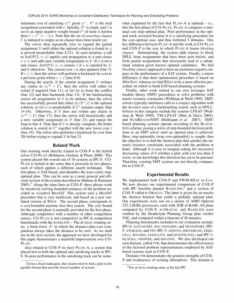
Experimental ResultsWe implemented both COS-P and PWM-RSAT in C++.We now discuss our experimental comparison of COS-Pwith IPC baseline planner BASELINE,6 and a version ofCOS-P called H-ORACLE. The latter is given (by an oracle)the shortest horizon that yields a globally optimal plan.Our experiments were run on a cluster of AMD Opteron252 2.6GHz processors, each with 2GB of RAM. All planscomputed by COS-P, H-ORACLE, and BASELINE wereverified by the Strathclyde Planning Group plan verifierVAL, and computed within a timeout of 30 minutes.

Planning benchmarks included in our evaluation include:IPC-6: ELEVATORS, PEG SOITAIRE, and TRANSPORT; IPC-5: STORAGE, and TPP; IPC-3: DEPOTS, DRIVERLOG, FREE-CELL, ROVERS, SATELLITE, and ZENOTRAVEL; and IPC-1:BLOCKS, GRIPPER, and MICONIC. We also developed ourown domain, called FTB, that demonstrates the effectivenessof the factored problem representations employed by SAT-based systems such as COS-P.

Domain FTB demonstrates the greatest strengths of COS-P and weaknesses of existing alternatives. This domain is

6The de facto winning entry at the last IPC.


19

based on the worst-case problem from (Hoey et al. 1999).FTB domain features one type of problem object, each withstatus achieved or unachieved. In a starting stateall have status unachieved. Objects are grouped into nclasses of equal size, and each class determines a total-orderδi over its objects. For each object we have a zero-cost ac-tion that will unachieved that object in any state. An-other zero-cost action will make an object from the ith classachieved provided its immediate successor according toδi is achieved.7 We also have n actions s-actioni eachof which makes the least object according to δi achieved,and which can only be executed in the starting state. Thereare corresponding actions g-actioni that make the goaltrue provided all objects in the ith class are achieved.For increasing i the cost of s-actioni is non-zero mono-tonically decreasing, and non-zero monotonically increas-ing for g-actioni. For all i and j we have that the costof s-actioni is less than the cost of g-actionj . Fi-nally, we have two types of cheating action: (1) zero-cost ac-tion cheat-a, that can make any object achieved in anystate, and (2) cheat-g that makes the goal achieved, how-ever has an action cost grater than executing s-actioniand g-actioni for any i. Finally, we add a preconditionto actions g-actioni by have them forbidden if the agenthas executed a cheating action.

The important characteristics of ftb are as follows. First,problems have exponentially many states in the number ofproblem objects. Moreover, there is a severe branching fac-tor at each state. Consequently, a (heuristic) search in prob-lem state space —as performed by systems such as HSPand BASELINE— is not efficient. Also, for the same rea-son “worst-case” crippled ADD-based value-iteration tech-niques, ftb cripples BDD-based symbolic breadth-firstsearch along the lines of GAMER. Second, ftb containssome manner of a temporal cost assignment problem. In par-ticular, the cost of achieving the goal is a foregone conclu-sion after the agent has executed the first action. Therefore,systems that do not employ an effective heuristic – examplesinclude GAMER and BASELINE – are very inefficient.

The results of our experiments are summarised in Table 1.For each domain there is one row for the hardest probleminstance solved by each of the three planners. Here, we mea-sure problem hardness as the time it takes each solver to re-turn the optimal plan. In some domains we also include ad-ditional instances. Using the same experimental data as forTable 1, Figure 1 plots the cumulative number of instancessolved over time by each planning system, supposinginvocations of the systems on problem instances are madein parallel. It is important to note that the size of the CNFencodings required by COS-P (and H-ORACLE) are notprohibitively large – i.e, where the SAT-based approachesfail, this is typically because they exceed the 30 minutestimeout, and not because they exhaust system memory.

COS-P outperforms the BASELINE in the BLOCKS andFTB domains. For example, on BLOCKS-18 BASELINE

7Note, this domain admits optimal plans in the parallel formatwhich execute actions changing the achieved status of multipleobjects in parallel.

0

20

40

60

80

100

120

140

160

180

0.01 0.1 1 10 100 1000 10000

Pro

blem

s so

lved

Planning time (s)

Problems solved in parallel

BaselineHorizon Oracle

COS-P

Figure 1: The number of problems solved in parallel after agiven planning time for each approach.

takes 39.15 seconds while COS-P takes only 3.47 seconds.In other domains BASELINE outperforms COS-P, some-times by several orders of magnitude. For example, on prob-lem ZENOTRAVEL-4 BASELINE takes 0.04 seconds whileCOS-P takes 841.2. More importantly, we discovered that itis relatively easy to find a cost-optimal solution compared toproving its optimality. For example, on MICONIC-23 COS-P took 0.53 seconds to find the optimal plan but spent 1453seconds proving cost optimality. More generally, this obser-vation is indicated by the performance of H-ORACLE.

Overall, we find that clause learning procedures inPWM-RSAT cannot exploit the presence of the very ef-fective delete relaxation heuristic from Π+. Consequently,a serious bottleneck of our approach comes from the timerequired to solve VARIANT-II instances. On a positivenote, those proofs are possible, and in domains such asBLOCKS and FTB, where the branching factor is high anduseful plans long, the factored problem representations andcorresponding solution procedures in the SAT-based settingpayoff. Moreover, in fixed-horizon cost-optimal planning,the SAT approach continues to show good performancecharacteristics in many domains.

Concluding RemarksIn this paper we demonstrate that a general theorem-provingtechnique, particularly a DPLL procedure for Boolean SAT,can be modified to find cost-optimal solutions to proposi-tional planning problems encoded as SAT. This was sup-posed to be possible, although in a very impractical sense, inthe final remarks of (Giunchiglia & Maratea 2007). In par-ticular, we modified SAT solver RSAT2.02 to create PWM-RSAT, an effective partial weighted MaxSAT procedure forproblems where all soft constraints are unit clauses. Thisforms the underlying optimisation procedure in COS-P, ourcost-optimal planning system that, for successive horizonlengths, uses PWM-RSAT to establish a candidate solutionat that horizon, and then to determine if that candidate isglobally optimal. Each candidate is a minimal cost step-bounded plan for the problem at hand. That a candidate is


20

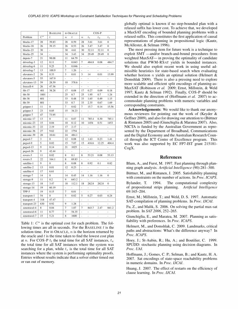
BASELINE H-ORACLE COS-P

Problem C∗ t n t n tt tπ t∗

blocks-17 28 39.83 28 0.59 28 3.61 3.61 0

blocks-18 26 39.15 26 0.53 26 3.47 3.47 0

blocks-23 30 - 30 4.61 30 32.11 32.11 0

blocks-25 34 - 34 3.43 34 29.49 29.49 0

depots-7 21 98.08 11 64.79 - - - -

driverlog-3 12 0.11 7 0.043 7 484.8 0.08 484.7

driverlog-6 11 9.25 5 0.046 - - - -

driverlog-7 13 100.9 7 1.26 - - - -

elevators-2 26 0.33 3 0.01 3 14 0.01 13.99

elevators-5 55 167.9 - - - - - -

elevators-13 59 28.59 10 378.6 - - - -

freecell-4 26 47.36 - - - - - -

ftb-17 401 38.28 17 0.08 17 0.27 0.09 0.18

ftb-30 1001 - 25 0.7 25 1.95 0.7 1.24

ftb-38 601 - 33 0.48 33 1.65 0.49 1.15

ftb-39 801 - 33 0.7 33 2.35 0.67 1.69

gripper-1 11 0 7 0.02 7 15.7 0.14 15.56

gripper-3 23 0.05 15 34.23 - - - -

gripper-7 47 73.95 - - - - - -

miconic-17 13 0 11 0.07 11 785.4 0.30 785.1

miconic-23 15 0.04 10 0.12 10 1454 0.51 1453

miconic-33 22 2.19 17 2.17 - - - -

miconic-36 27 9.62 22 1754 - - - -

miconic-39 28 10.61 24 484.1 - - - -

pegsol-7 3 0 12 0.08 12 1.63 0.23 1.41

pegsol-9 5 0.02 15 7.07 15 416.6 12.25 404.4

pegsol-13 9 0.14 21 1025 - - - -

pegsol-26 9 42.44 - - - - - -

rovers-3 11 0.02 8 0.1 8 53.21 0.08 53.13

rovers-5 22 164.1 8 69.83 - - - -

satellite-1 9 0 8 0.08 8 0.92 0.1 0.82

satellite-2 13 0.01 12 0.23 - - - -

satellite-4 17 6.61 - - - - - -

storage-7 14 0 14 0.45 14 1.16 1.16 0

storage-9 11 0.2 9 643.2 - - - -

storage-13 18 3.47 18 112.1 18 262.8 262.8 0

storage-14 19 60.19 - - - - - -

TPP-5 19 0.15 7 0.01 - - - -

transport-1 54 0 5 0.02 5 0.27 0.03 0.24

transport-4 318 47.47 - - - - - -

transport-23 630 0.92 9 1.28 - - - -

zenotravel-4 8 0.04 7 1.07 7 843.7 2.47 841.2

zenotravel-6 11 8.77 7 54.35 - - - -

zenotravel-7 15 5.21 8 1600 - - - -

Table 1: C∗ is the optimal cost for each problem. The fol-lowing times are all in seconds. For the BASELINE t is thesolution time. For H-ORACLE, n is the horizon returned bythe oracle and t is the time taken to find the lowest cost planat n. For COS-P tt the total time for all SAT instances, tπthe total time for all SAT instances where the system wassearching for a plan, while t∗ is the total time for all SATinstances where the system is performing optimality proofs.Entries without results indicate that a solver either timed outor ran out of memory.

globally optimal is known if no step-bounded plan with arelaxed suffix has lower cost. To achieve that, we developeda MaxSAT encoding of bounded planning problems with arelaxed suffix. This constitutes the first application of causalrepresentations of planning in propositional logic (Kautz,McAllester, & Selman 1996).

The most pressing item for future work is a technique toexploit SMT —and/or branch-and-bound procedures fromweighted MaxSAT— in proving the optimality of candidatesolutions that PWM-RSAT yields in bounded instances.We should also exploit recent work in using useful ad-missible heuristics for state-based search when evaluatingwhether horizon n yields an optimal solution (Helmert &Domshlak 2009). There is also a pressing need to exploremore scalable and efficient split encodings of planning-as-MaxSAT (Robinson et al. 2009; Ernst, Millstein, & Weld1997; Kautz & Selman 1992). Finally, COS-P should beextended in the direction of (Hoffmann et al. 2007) to ac-commodate planning problems with numeric variables andcorresponding constraints.

Acknowledgements: We would like to thank our anony-mous reviewers for pointing out the work of (Keyder &Geffner 2009), and also for drawing our attention to (Buttner& Rintanen 2005) and (Giunchiglia & Maratea 2007). Also,NICTA is funded by the Australian Government as repre-sented by the Department of Broadband, Communicationsand the Digital Economy and the Australian Research Coun-cil through the ICT Centre of Excellence program. Thiswork was also supported by EC FP7-IST grant 215181-CogX.

ReferencesBlum, A., and Furst, M. 1997. Fast planning through plan-ning graph analysis. Artificial Intelligence (90):281–300.

Buttner, M., and Rintanen, J. 2005. Satisfiability planningwith constraints on the number of actions. In Proc. ICAPS.

Bylander, T. 1994. The computational complexityof propositional strips planning. Artificial Intelligence69:165–204.

Ernst, M.; Millstein, T.; and Weld, D. S. 1997. AutomaticSAT-compilation of planning problems. In Proc. IJCAI.Fu, Z., and Malik, S. 2006. On solving the partial max-satproblem. In SAT 2006, 252–265.

Giunchiglia, E., and Maratea, M. 2007. Planning as satis-fiability with preferences. In Proc. ICAPS.

Helmert, M., and Domshlak, C. 2009. Landmarks, criticalpaths and abstractions: What’s the difference anyway? InProc. ICAPS.

Hoey, J.; St-Aubin, R.; Hu, A.; and Boutilier, C. 1999.SPUDD: stochastic planning using decision diagrams. InProc. UAI.Hoffmann, J.; Gomes, C. P.; Selman, B.; and Kautz, H. A.2007. Sat encodings of state-space reachability problemsin numeric domains. In Proc. IJCAI.Huang, J. 2007. The effect of restarts on the efficiency ofclause learning. In Proc. IJCAI.


21

Josep Argelic and, C. M. L.; Manya, F.; and Planes, J.2008. The first and second max-sat evaluations. Journal onSatisfiability, Boolean Modeling and Computation 4:251–278.

Kautz, H., and Selman, B. 1992. Planning as satisfiability.In Proc. ECAI.Kautz, H., and Selman, B. 1999. Unifying SAT-based andgraph-based planning. In Proc. IJCAI.Kautz, H.; McAllester, D.; and Selman, B. 1996. Encodingplans in propositional logic. In Proc. KR.

Kautz, H. A. 2006. Deconstructing planning as satisfiabil-ity. In Proc. AAAI.Keyder, E., and Geffner, H. 2009. Soft goals can becompiled away. Journal of Artificial Intelligence Research36(1).

Marques-Silva, J. P., and Sakallah, K. A. 1996. Grasp - anew search algorithm for satisfiability. In Proc. ICCAD.

Moskewicz, M. W.; Madigan, C. F.; Zhao, Y.; Zhang, L.;and Malik, S. 2001. Chaff: Engineering an Efficient SATSolver. In Proc. DAC.

Pipatsrisawat, K., and Darwiche, A. 2007. Rsat 2.0: SATsolver description. Technical Report D–153, AutomatedReasoning Group, Computer Science Department, UCLA.

Rintanen, J. 2004. Evaluation strategies for planning assatisfiability. In Proc. ECAI.Rintanen, J. 2008. Planning graphs and propositionalclause learning. In Proc. KR.

Robinson, N.; Gretton, C.; Pham, D. N.; and Sattar, A.2009. Sat-based parallel planning using a split representa-tion of actions. In Proc. ICAPS.

Robinson, N.; Gretton, C.; and Pham, D.-N. 2008.Co-plan: Combining SAT-based planning with forward-search. In Proc. IPC-6.

Russell, R., and Holden, S. 2010. Handling goal utilitydependencies in a satisfiability framework. In Proc. ICAPS.

Shin, J.-A., and Davis, E. 2005. Processes and continuouschange in a sat-based planner. Artif. Intell. 166(1-2):194–253.

Streeter, M., and Smith, S. 2007. Using decision proce-dures efficiently for optimization. In Proc. ICAPS.

Wolfman, S. A., and Weld, D. S. 1999. The LPSAT engineand its application to resource planning. In Proc. IJCAI.


22

A Pseudo-Boolean approach for Solving Planning Problems withIPC Simple Preferences

Enrico Giunchiglia and Marco MarateaDIST - University of Genova, Viale F. Causa 15, Genova, Italy

{enrico,[email protected]}

Abstract

Planning as Satisfiability (SAT) is the best approach to opti-mally solve classical planning problems in term of makespan,as witnessed by the results of past International PlanningCompetitions (IPCs). The language of the IPCs has evolvedin the last two editions in order to include plan quality mea-sures other than the makespan, e.g., to include “preferences”for the satisfaction of actions preconditions and/or goals:yet, the design, implementation and analysis of satisfiability-based approaches to cope with this issues is still at an earlystage. In this paper, motivated by the recent availability ofefficient systems to solve Pseudo-Boolean (PB) optimizationproblems, we present an approach to solve the instances inthe “SimplePreferences” category of the IPC-5 by a reduc-tion to a PB formula, and then use off-the-shelf PB solvers.Our approach thus returns plans with optimal plan metrics,at fixed makespan. We prove that the approach is correct,and then show that an implementation of our ideas based onSATPLAN yields to an effective method to solve these IPC-5benchmarks.

IntroductionPlanning as Satisfiability (SAT) is the best approach tooptimally solve classical planning problems in term ofmakespan, as witnessed by the results of past InternationalPlanning Competitions (IPCs): two SAT-based planners,namely SATPLAN1 (Kautz and Selman 1999; 2006) andMAXPLAN2 (Xing, Chen, and Zhang 2006a; Chen et al.2009), have been the winners in the “optimal” track of thedeterministic part of the IPC-43 (Hoffmann and Edelkamp2005) and IPC-54 (Gerevini et al. 2009). The languageof the IPCs has evolved in the last two editions in orderto include plan quality measures other than the makespan,e.g., to include “preferences” for the satisfaction of actionspreconditions and/or goals. Instead, the work on satisfia-bility planning has mainly focused of enhancing the effi-

Copyright c© 2010, Association for the Advancement of ArtificialIntelligence (www.aaai.org). All rights reserved.

1Available at http://www.cs.rochester.edu/˜kautz/satplan/index.htm .

2Available at http://www.cse.wustl.edu/˜chen/maxplan/.

3http://www.tzi.de/˜edelkamp/ipc-4/.4http://zeus.ing.unibs.it/ipc-5/.

ciency of the SAT-based approach with improved encod-ings, see, e.g., (Rintanen, Heljanko, and Niemela 2006;Chen et al. 2009), and the exceptions to this trend are limitedto somehow particular form of preferences and plan qualitymeasures (e.g., soft goals with uniform costs (Giunchigliaand Maratea 2007), minimum-length plans (Buttner andRintanen 2005), actions costs (Ramirez and Geffner 2007;Chen, Lv, and Huang 2008)). Thus, the design, implementa-tion and analysis of satisfiability-based approaches to copewith the mentioned plan quality issues is still at an earlystage.

In this paper, motivated by the recent availability of ef-ficient systems to solve Pseudo-Boolean (PB) optimizationproblems, which is the result of a series of PB evaluations5,we present an approach to solve the instances in the “Sim-plePreferences” category of the IPC- 5 by a reduction to aPB formula, and then using off-the-shelf PB solvers: suchdomains contain preferences on goals and/or actions precon-ditions, and there is a cost associated to the violation of suchpreferences. The reduction is carried out in two steps: giventhat such IPC-5 benchmarks are non-STRIPS, and someADL constructs are used, we first compile IPC-5 bench-marks into STRIPS problems, by using the ADL2STRIPS

tool6, and then generate PB formulas from the STRIPS prob-lems. A PB formulation in a very natural and concise wayto express such optimization problems, and result in (muchmore) compact formulas than SAT.

Our approach thus returns plans with optimal plan met-ric, at fixed makespan. It has to be noted that there al-ready exist in the context of optimal planning works thatuse optimization problems: a Max-SAT formulation hasbeen used in, e.g., (Xing, Chen, and Zhang 2006b), butfor the minimization of the makespan. Also, a modelingof planning problems with preferences, expressed throughthe PDDL3.0 (Gerevini et al. 2009) language, in 0-1 IntegerProgramming has been presented in (van den Briel, Kamb-hampati, and Vossen 2006). However, the first paper doesnot take into account the new features/metrics of PDDL,while in the second paper no implementation and experi-

5See http://www.cril.univ-artois.fr/PB09/ forthe last.

6Specifically, we have used the version based on LPG (see,e.g., (Gerevini and Serina 1999; Gerevini, Saetti, and Serina 2003),provided by Alessandro Saetti, which is the one used in the IPC-5.


23

mental analysis are provided; moreover, both papers do notcontain any formal result.

We first prove that the approach is correct. Then, weshow that an implementation of our ideas based on SAT-PLAN yields to an effective method to solve the instancesin the “SimplePreferences” category of the IPC-5, by tak-ing as reference the results of SGPLAN (Hsu et al. 2006;2007), the clear winner of the IPC-5 in this category.

Given that in the IPC-5 the impact of preferencesviolation on the plan metric is restricted to be linear, wefocus on this case. Thus, all results we present couldbe simply adapted to work with an approach based onpartial weighted Max-SAT, an extension of the well-knownMax-SAT problem in which there are “hard” and “soft”clauses, and the goal is to find an assignment that satisfiesall hard clauses and maximize the sum of the weights ofsatisfied soft clauses. Still, we present an analysis where aPB solver, namely MINISAT+ (Een and Sorensson 2006),is the best, among a variety of PB and Max-SAT solvers,on the instances of interest. This is interesting, given thatPB, in general, is a richer formalism than partial weightedMax-SAT.

Summing up, the major contributions of the paperare:

• We present an approach based on PB for handling IPC-5 “SimplePreferences” benchmarks within a satisfiabilityframework;

• We prove that the approach is correct;

• We implement these ideas in SATPLAN, and show thatthe approach is viable, i.e., it allows to widening the setof benchmarks can be dealt with a satisfiability-basedapproach.

The paper is structured as follows. We first present theneeded preliminaries. Then, the following sections focuson how we model and solve the problem of interest. De-tails about the implementation, and the experimental evalu-ation, are then presented. The paper ends with discussion ofrelated works and with conclusions and possible topics forfuture research.

PreliminariesLet F and A be the set of fluents and actions, respectively.A state is an interpretation of the fluent signature. A com-plex action α, i.e., a set of actions, is an interpretation of theaction signature, and models the concurrent execution of theactions satisfied by α, i.e., it is a set of actions that can beexecuted in parallel.A planning problem is a triple 〈I, tr,G〉 where

• I is a Boolean formula over F and represents the initialstate;

• tr is a Boolean formula over F∪A∪F ′ where F ′ = {f ′ :f ∈ F} is a copy of the fluent signature and representsthe transition relation of the automaton describing how(complex) actions affect states (we assume F ∩ F ′ = ∅);

• G is a Boolean formula over F and represents the set ofgoal states.

In the above definition of a planning problem, actions’ ef-fects on a state are described in an high-level action languagelike STRIPS (Fikes and Nilsson 1971), or PDDL. Given thatthe focus of our work is on classical planning, we make theassumption that the description is deterministic: the execu-tion of a (complex) action α in a state s can lead to at mostone state s′. More formally, for each state s and complexaction α there is at most one interpretation extending s ∪ αand satisfying tr.

Consider a planning problem Π = 〈I, tr,G〉. In the fol-lowing, for any integer i:

• if F is a formula in the fluent signature, Fi is obtainedfrom F by substituting each f ∈ F with fi; and

• tri is the formula obtained from tr by substituting eachsymbol p ∈ F ∪ A with pi−1 and each f ∈ F ′ with fi.

In the planning as satisfiability approach (Kautz and Sel-man 1992), if n is an integer, the planning problem Π withmakespan n is the Boolean formula Πn defined as

I0 ∧n∧

i=1

tri ∧Gn, n ≥ 0 (1)

and a plan is an interpretation satisfying (1). 7

In a linear PB optimization problem, SAT clauses (i.e., setof literals) are extended to possibly contain integer coeffi-cients, variables truth/falsity is interpreted as 0/1, and thereis a bound on the value the constraint can assume. Givena set of coefficients c1, . . . , ck, a set of boolean variables{x1, . . . , xk}, and a positive integer number b, a PB con-straint is of the form:

k∑

i=1

ci × xi ≥ b (2)

A PB formula is a conjunction of PB constraints. Moreover,an objective function can be applied8 to the problem. If suchobjective function is specified, given a PB formula ϕPBn thegoal is to find an assignment to the variables of the problemthat satisfies the formula (i.e., all PB constraints are satis-fied), and optimizes the objective function.

Modeling IPC Simple Preferences problems asPB problems

As we said in the introduction, the reduction to a PB formulais carried out in two steps: SATPLAN, the planner we relyon, can only handle STRIPS problems, while IPC-5 bench-marks contain some ADL constructs to represent prefer-ences. Thus, the first step is to adapt the IPC-5 benchmarks

7In the following, we can switch between plans and satisfyinginterpretations, intuitively meaning the same thing. In SAT, an in-terpretation is a set of literals; in PB, is an assignment of variablesto 0 (i.e., falsity) or 1 (i.e., truth). It is easy to map interpretationsinto assignments and viceversa.

8In fact, in the PB evaluations the categories take into accountif such function is specified (OPT), or not (DEC).


24

in a way that can be compiled into a STRIPS problem bystate-of-the-art tools, e.g., ADL2STRIPS. For presenting ourapproach, we rely on the instance #1 of the TPP (Travellingand Purchase Problem) domain of the IPC-5, which con-tains preferences on both actions preconditions and goals,“GroundedPreferences” variant (referred as tpp1 below). Inthe following, we show the part related to the treatment ofpreferences, and how they have been modeled in PB. All theother SAT clauses are translated into PB constraints. In tpp1,action “drive” is represented as follows

(:action drive:parameters (?t - truck ?from ?to - place):precondition (and (at ?t ?from) (connected ?from ?to)

(preference p-drive (and(ready-to-load goods1 ?from level0)(ready-to-load goods2 ?from level0)(ready-to-load goods3 ?from level0))))

:effect (and (not (at ?t ?from)) (at ?t ?to)))(3)

(Soft) Goals and the metric are represented with

(:goal (and(preference p4A

(and (ready-to-load goods3 market1 level0)(loaded goods3 truck1 level0)))

...(preference p0A (stored goods3 level1))...

))

(:metric minimize (+ (* 1 (is-violated p0A))...(* 16 (is-violated p4A))(* 1 (is-violated p-drive))))

(4)The semantic is defined as follows (Gerevini et al. 2009):in (3), action “drive” can be executed even if preference “p-drive” is violated, but then a cost 1 (from (4)) is paid eachtime this happens; in (4), the related cost in the metric is paidif any of the goal preference is violated.

We first modify the problem, in a way which is in-spired by the approaches in (Gazen and Knoblock 1997;Benton, Kambhampati, and Do 2006), in order to avoid theuse of the construct “preference”: for each goal preferencewe introduce a (dummy) action whose precondition is thepreference, and the effect is a (dummy) literal, e.g., for pref-erence p4A

(:action dummy-p4A:parameters ():precondition (and (ready-to-load goods3 market1 level0)

(loaded goods3 truck1 level0)):effect (and (goal-p4A))).

(5)

The new (hard) goal of the problem is the conjunction of thedummy literals related to goal preferences introduced.Note that, in PDDL3.0, several preferences can be taggedwith the same preference name, and the same cost is associ-ated to each single violation. This is indeed the case for the

instances in the TPP domain (“GroundedPreferences” vari-ant).

Actions containing preferences their preconditions, aresplit into two actions: the first, which we consider to main-tain its name, consider the soft precondition in the action“drive” as hard; then, we introduce a second (dummy) ac-tion of the form9

(:action dummydr:parameters (?t - truck ?from ?to - place):precondition (and (at ?t ?from) (connected ?from ?to)

(not (and(ready-to-load goods1 ?from level0)(ready-to-load goods2 ?from level0)(ready-to-load goods3 ?from level0))))

:effect (and (not (at ?t ?from)) (at ?t ?to) (goal-p-drive)))(6)

where the soft precondition of the related original actionis negated, and a dummy literal is added to the original ef-fects. The intuition is to take into account if the originalaction is executed with, or without, its precondition formulasatisfied: in this second case, goal-p-drive is added as afurther effect. The two actions are mutually exclusive: thesecond takes into account if action drive is executed with itssoft precondition not satisfied.

The resulting problem is then given to the ADL2STRIPS

tool to be compiled into a STRIPS problem. Dummy actionsintroduced are thus compiled into STRIPS actions. Thus,there could be (multiple) STRIPS actions in place of theones in (5) or (6), whose preconditions (resp. effects) arefinite conjunction of atoms (resp. literals). Below, such con-junction can be (equivalently) considered as sets.

Consider a STRIPS problem (with variable names possi-bly equal to the non-STRIPS problem). Further, let ϕdr bethe preference formula related to “p-drive”, ϕh is the for-mula corresponding to the “hard” part of the preconditionsof the action “drive”, and ϕe its effects, the following PBconstraints are added to the PB problem.

Given a non-STRIPS action A-p, in the following wewrite Ap,i for (one of) the corresponding STRIPS actionwith subscript, or time-stamp, i. Given that in the tpp1 in-stance there are 5 (0 ≤ j ≤ 4) soft goals, for each STRIPSaction related to goals (5) (in PB-like format, without “×”)

∧l∈ϕjA,n−1 − 1 dummypjA,n−1 + 1 ln−1 ≥ 0,

−1 dummypjA,n−1 + 1 goalpjA,n ≥ 0Regarding action drive, the following PB constraints are

added (we remind that its preconditions are all hard)

∧l∈ϕh− 1 drivei + 1 li ≥ 0,

∧l∈ϕdr− 1 drivei + 1 li ≥ 0

while, for the effects, the following constraints are added

∧l∈ϕe− 1 drivei + sign(l) var(l)i+1 ≥ bl

where var(l) returns the (fluent) variable the literal is builton, and sign(l) is 1 and bl is 0 if the literal is positive, while

9We can introduce a single action given that only one preferenceformula is in action “drive”. This is the case for all instances inthe “SimplePreferences” category. In general, we have to considertheir power set.


25

sign(l) is −1 and bl is −1, otherwise. The last PB constraintadded is

−1 drivei + 1 goalp−drive,i+1 ≥ 0Similarly for action dummydr (5).

Now, it is left how to express the optimization function:in (4), the idea is to minimize the violation of prefer-ences (expressed with constructs (is-violated p) in PDDL3.0,where, given a preference p, (is-violated p) takes value 1 ifthe preference is not satisfied, and 0 otherwise (Gerevini etal. 2009)). With our formulation, the new goal literals ofintroduced actions are reached when a preference is satis-fied and this is “mimicked” by the related action’s execu-tion: thus, the characterization of the metric function in (4)can be expressed using both actions and goals, i.e. with thefollowing (linear) optimization functions (without subscript“A” in the equations)

max: +1 (goalp0) + . . . +16 (goalp4) +∑ni=1 −1 (goaldr,i)

(7)max:+1 (dummyp0)+ . . . +16 (dummyp4)+

∑n−1i=o −1(dummydr,i)

(8)with the meaning that goal (resp. dummy) takes value

1 if it holds (resp. is executed) at that time stamp, and0 otherwise. While literals referred the goal preferences,i.e., {goalp0A, . . . , goalp4A} in (7), (resp., dummy actions,i.e., {dummyp0A, . . . , dummyp4A}) can hold only at timestamp n (resp. n − 1), the ones related to action precondi-tions can, in general, hold at any time stamp (in (7) and (8)such subscripts are implicit). If we know that, instead, ac-tions can be only executed once, the optimization functionthat uses goals is expressed with

max: +1 (goalp0) + . . . + 16 (goalp4) −1 (goaldr) (9)

and similarly for (8). Even if from one hand this hypothe-sis on (ground) actions execution underlying (9) can be seenas a further approximation (other than the makespan) of the(unbounded) optimal plan metric, such hypothesis hold inpractice in various cases, e.g., on classical, real-world plan-ning domain like blocks-world and logistics.

A PB-based Solving AlgorithmConsider a STRIPS problem Π, and an integer n; P is theset of atoms added as effects in the actions introduced (P ={goalp0A, . . . , goalp4A, goaldr} in (9)), and c is a functionthat maps elements in P with their corresponding positiveinteger costs.10

In Figure 1 there is the solving algorithm, in which

10We can restrict to positive integer costs given that: (i) IPC-5 benchmarks do not contain negative weights, and (ii) positivereal costs of the IPC-5 can be represented with integer numbersby multiplying them by 10d, where d is the maximum number of(significant) decimal digits in the problem. However, dealing withnegative costs is not a problem: assuming that c(p) < 0 for somep ∈ P , we can replace p with ¬p in P and define c(¬p) = −c(p):the set of optimal plans does not change. Given 〈P, c〉, we canconsider the quantitative preference 〈P ′, c′〉 where P ′ = {¬p :p ∈ P} with c′(¬p) = c(p), and then look for a plan maximizingP

p∈P ′:π|=p c′(p).

function PBPLAN(Π,n,P ,c)1 return PBO(CNF2PB(CNF(Πn)), μ, o)

Figure 1: The algorithm of PBPLAN.

• CNF(ϕ), where ϕ is a formula, is a set of clauses such that

– for any interpretation μ′ in the signature of CNF(ϕ)such that μ′ |= CNF(ϕ) it is true also that μ |= ϕ, whereμ is the interpretation μ′ but restricted to the signatureof ϕ; and

– for any interpretation μ |= ϕ there exists an interpreta-tion μ′, μ′ ⊇ μ, such that μ′ |= CNF(ϕ).

There are well-known methods for computing CNF(ϕ)in linear time by introducing additional variables,e.g., (Tseitin 1970; Plaisted and Greenbaum 1986; Jack-son and Sheridan 2005);

• CNF2PB(C), where C = {l1 . . . lm} is a clause, is a PBconstraint p = c1 × x1 + . . . + cm × xm ≥ b where,for each k, 1 ≤ k ≤ m, ck = +1 and xk = lk if lkis a positive literal, while ck = −1 and xk = var(lk) iflk is a negative literal, with b = 1 − count(c1, . . . , cm),where count(c1, . . . , cm) returns the number of negativecoefficients; p is such that

– for any interpretation μ, μ |= C, there is an assignmentto integer variables in p such that p is satisfied; and

– for any assignment to the integer variables in p that sat-isfies the constraint, there is an interpretation μ suchthat μ |= C.

CNF2PB(φ), where φ is a set of clauses, is∧

C∈φCNF2PB(C)

• o(ϕ) is the optimization function, of the form (7)-(9), thus

max :∑

p∈P ′c′(p) × p.

where

– P ′ = P and c′ = c, if we deal with an optimizationfunction of type (9); or

– P ′ = P ∪n−1i=1 {goaldr,i} and c′ extends c by assigning

atoms in P ′ \P the weight c(goaldr,n), if we deal withan optimization function of type (7) (atoms in P areimplicitly with subscript n). Similarly for (8).

Consider ΠPBn to be a PB formula, and PBO a generic

PB solver, which returns FALSE if ΠPBn is unsatisfiable,

or a solution μ, which satisfies ΠPBn and maximizes o,

otherwise.

We are now ready to state the following Theorem.

Theorem 1 Let Π be a planning problem, n the makespan,P the set of variables involved in the metric, with function c.PBPLAN(Π,n,P ,c) returns


26

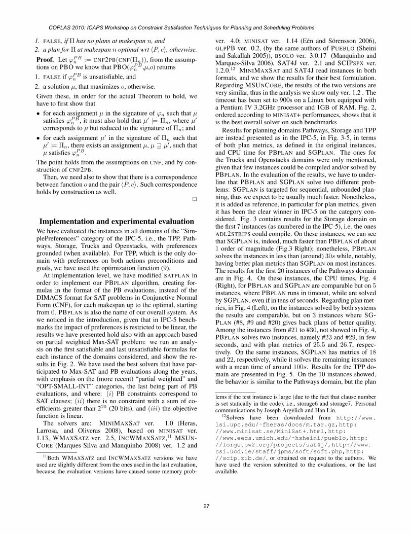
1. FALSE, if Π has no plans at makespan n, and2. a plan for Π at makespan n optimal wrt 〈P, c〉, otherwise.

Proof. Let ϕPBn := CNF2PB(CNF(Πn)), from the assump-tions on PBO we know that PBO(ϕPBn ,μ,o) returns

1. FALSE if ϕPBn is unsatisfiable, and

2. a solution μ, that maximizes o, otherwise.

Given these, in order for the actual Theorem to hold, wehave to first show that

• for each assignment μ in the signature of ϕn such that μsatisfies ϕPBn , it must also hold that μ′ |= Πn, where μ′corresponds to μ but reduced to the signature of Πn; and

• for each assignment μ′ in the signature of Πn such thatμ′ |= Πn, there exists an assignment μ, μ ⊇ μ′, such thatμ satisfies ϕPBn .

The point holds from the assumptions on CNF, and by con-struction of CNF2PB.

Then, we need also to show that there is a correspondencebetween function o and the pair 〈P, c〉. Such correspondenceholds by construction as well.

�

Implementation and experimental evaluationWe have evaluated the instances in all domains of the “Sim-plePreferences” category of the IPC-5, i.e., the TPP, Path-ways, Storage, Trucks and Openstacks, with preferencesgrounded (when available). For TPP, which is the only do-main with preferences on both actions preconditions andgoals, we have used the optimization function (9).

At implementation level, we have modified SATPLAN inorder to implement our PBPLAN algorithm, creating for-mulas in the format of the PB evaluations, instead of theDIMACS format for SAT problems in Conjunctive NormalForm (CNF), for each makespan up to the optimal, startingfrom 0. PBPLAN is also the name of our overall system. Aswe noticed in the introduction, given that in IPC-5 bench-marks the impact of preferences is restricted to be linear, theresults we have presented hold also with an approach basedon partial weighted Max-SAT problem: we run an analy-sis on the first satisfiable and last unsatisfiable formulas foreach instance of the domains considered, and show the re-sults in Fig. 2. We have used the best solvers that have par-ticipated to Max-SAT and PB evaluations along the years,with emphasis on the (more recent) “partial weighted” and“OPT-SMALL-INT” categories, the last being part of PBevaluations, and where: (i) PB constraints correspond toSAT clauses; (ii) there is no constraint with a sum of co-efficients greater than 220 (20 bits), and (iii) the objectivefunction is linear.

The solvers are: MINIMAXSAT ver. 1.0 (Heras,Larrosa, and Oliveras 2008), based on MINISAT ver.1.13, WMAXSATZ ver. 2.5, INCWMAXSATZ,11 MSUN-CORE (Marques-Silva and Manquinho 2008) ver. 1.2 and

11Both WMAXSATZ and INCWMAXSATZ versions we haveused are slightly different from the ones used in the last evaluation,because the evaluation versions have caused some memory prob-

ver. 4.0; MINISAT ver. 1.14 (Een and Sorensson 2006),GLPPB ver. 0.2, (by the same authors of PUEBLO (Sheiniand Sakallah 2005)), BSOLO ver. 3.0.17 (Manquinho andMarques-Silva 2006), SAT4J ver. 2.1 and SCIPSPX ver.1.2.0.12 MINIMAXSAT and SAT4J read instances in bothformats, and we show the results for their best formulation.Regarding MSUNCORE, the results of the two versions arevery similar, thus in the analysis we show only ver. 1.2 . Thetimeout has been set to 900s on a Linux box equipped witha Pentium IV 3.2GHz processor and 1GB of RAM. Fig. 2,ordered according to MINISAT+ performances, shows that itis the best overall solver on such benchmarks

Results for planning domains Pathways, Storage and TPPare instead presented as in the IPC-5, in Fig. 3-5, in termsof both plan metrics, as defined in the original instances,and CPU time for PBPLAN and SGPLAN. The ones forthe Trucks and Openstacks domains were only mentioned,given that few instances could be compiled and/or solved byPBPLAN. In the evaluation of the results, we have to under-line that PBPLAN and SGPLAN solve two different prob-lems: SGPLAN is targeted for sequential, unbounded plan-ning, thus we expect to be usually much faster. Nonetheless,it is added as reference, in particular for plan metrics, givenit has been the clear winner in IPC-5 on the category con-sidered. Fig. 3 contains results for the Storage domain onthe first 7 instances (as numbered in the IPC-5), i.e. the onesADL2STRIPS could compile. On these instances, we can seethat SGPLAN is, indeed, much faster than PBPLAN of about1 order of magnitude (Fig.3 Right); nonetheless, PBPLAN

solves the instances in less than (around) 30s while, notably,having better plan metrics than SGPLAN on most instances.The results for the first 20 instances of the Pathways domainare in Fig. 4. On these instances, the CPU times, Fig. 4(Right), for PBPLAN and SGPLAN are comparable but on 5instances, where PBPLAN runs in timeout, while are solvedby SGPLAN, even if in tens of seconds. Regarding plan met-rics, in Fig. 4 (Left), on the instances solved by both systemsthe results are comparable, but on 3 instances where SG-PLAN (#8, #9 and #20) gives back plans of better quality.Among the instances from #21 to #30, not showed in Fig. 4,PBPLAN solves two instances, namely #23 and #29, in fewseconds, and with plan metrics of 25.5 and 26.7, respec-tively. On the same instances, SGPLAN has metrics of 18and 22, respectively, while it solves the remaining instanceswith a mean time of around 100s. Results for the TPP do-main are presented in Fig. 5. On the 10 instances showed,the behavior is similar to the Pathways domain, but the plan

lems if the test instance is large (due to the fact that clause numberis set statically in the code), i.e., storage6 and storage7. Personalcommunications by Joseph Argelich and Han Lin.

12Solvers have been downloaded from http://www.lsi.upc.edu/˜fheras/docs/m.tar.gz,http://www.minisat.se/MiniSat+.html,http://www.eecs.umich.edu/˜hsheini/pueblo,http://forge.ow2.org/projects/sat4j/,http://www.csi.ucd.ie/staff/jpms/soft/soft.php,http://scip.zib.de/, or obtained on request to the authors. Wehave used the version submitted to the evaluations, or the lastavailable.


27

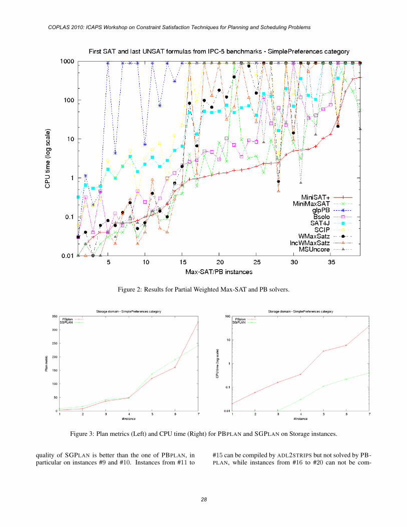
Figure 2: Results for Partial Weighted Max-SAT and PB solvers.

Figure 3: Plan metrics (Left) and CPU time (Right) for PBPLAN and SGPLAN on Storage instances.

quality of SGPLAN is better than the one of PBPLAN, inparticular on instances #9 and #10. Instances from #11 to

#15 can be compiled by ADL2STRIPS but not solved by PB-PLAN, while instances from #16 to #20 can not be com-


28

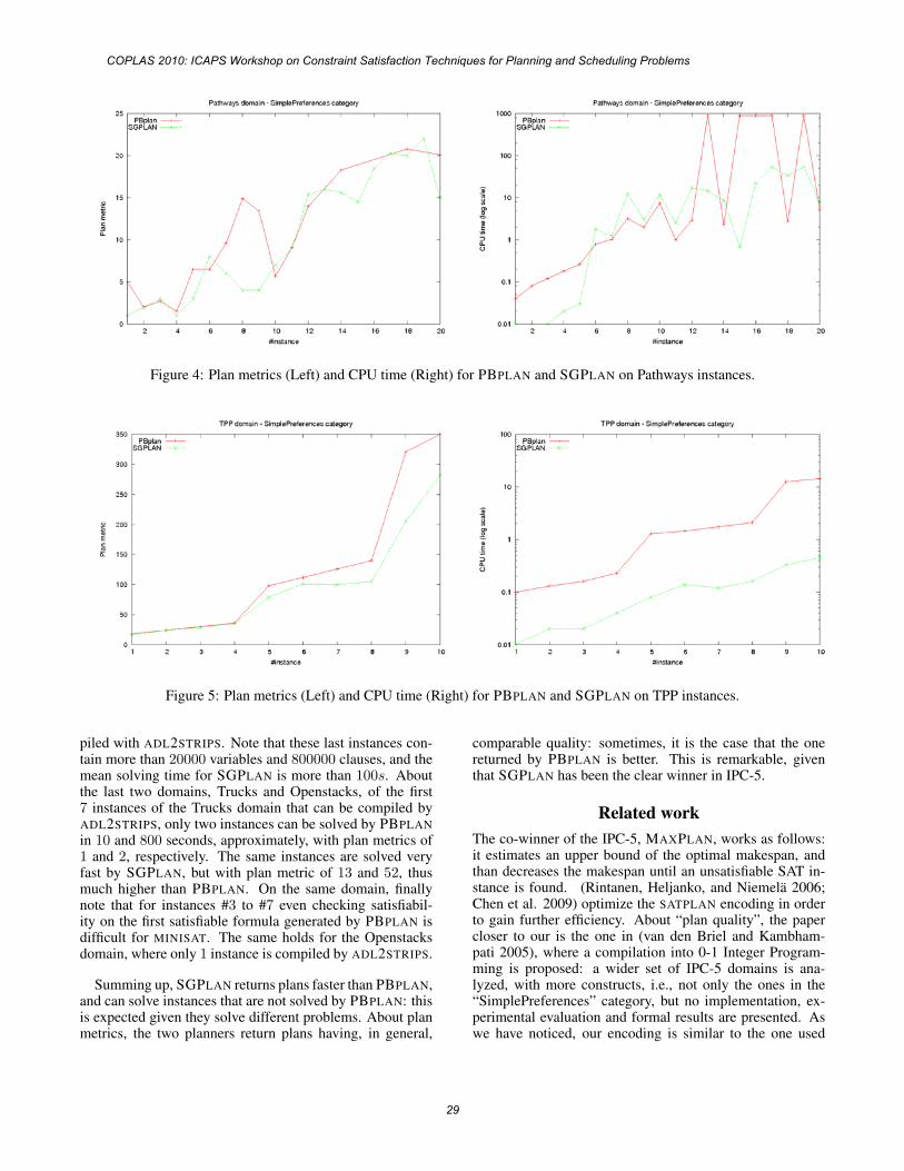
Figure 4: Plan metrics (Left) and CPU time (Right) for PBPLAN and SGPLAN on Pathways instances.

Figure 5: Plan metrics (Left) and CPU time (Right) for PBPLAN and SGPLAN on TPP instances.

piled with ADL2STRIPS. Note that these last instances con-tain more than 20000 variables and 800000 clauses, and themean solving time for SGPLAN is more than 100s. Aboutthe last two domains, Trucks and Openstacks, of the first7 instances of the Trucks domain that can be compiled byADL2STRIPS, only two instances can be solved by PBPLAN

in 10 and 800 seconds, approximately, with plan metrics of1 and 2, respectively. The same instances are solved veryfast by SGPLAN, but with plan metric of 13 and 52, thusmuch higher than PBPLAN. On the same domain, finallynote that for instances #3 to #7 even checking satisfiabil-ity on the first satisfiable formula generated by PBPLAN isdifficult for MINISAT. The same holds for the Openstacksdomain, where only 1 instance is compiled by ADL2STRIPS.

Summing up, SGPLAN returns plans faster than PBPLAN,and can solve instances that are not solved by PBPLAN: thisis expected given they solve different problems. About planmetrics, the two planners return plans having, in general,

comparable quality: sometimes, it is the case that the onereturned by PBPLAN is better. This is remarkable, giventhat SGPLAN has been the clear winner in IPC-5.

Related workThe co-winner of the IPC-5, MAXPLAN, works as follows:it estimates an upper bound of the optimal makespan, andthan decreases the makespan until an unsatisfiable SAT in-stance is found. (Rintanen, Heljanko, and Niemela 2006;Chen et al. 2009) optimize the SATPLAN encoding in orderto gain further efficiency. About “plan quality”, the papercloser to our is the one in (van den Briel and Kambham-pati 2005), where a compilation into 0-1 Integer Program-ming is proposed: a wider set of IPC-5 domains is ana-lyzed, with more constructs, i.e., not only the ones in the“SimplePreferences” category, but no implementation, ex-perimental evaluation and formal results are presented. Aswe have noticed, our encoding is similar to the one used


29

in YOCHANPS (Benton, Kambhampati, and Do 2006; Ben-ton, Do, and Kambhampati 2009): it compiles a PDDL3.0problem into a PSP planning problem (van den Briel et al.2004), which allows to add the cost of an action withinits definition. The compilation is, however, different fromour in the sense that it generates actions that are all appli-cable in states where all preferences are met, and actionsthat have cost may be inappropriately included in the plan atsuch states (from (Benton, Kambhampati, and Do 2006)),while for us this is not the case, by negating (soft) pre-conditions in one of the added actions. This would meanthat, in principle, the PSP compilation could produce incor-rect metric values, that have to be adjusted. Moreover, wealso provide a characterization of the metric functions de-fined on states, thus closer to the one of PDDL3.0 . Theworks in (Brafman and Chernyavsky 2005; Giunchiglia andMaratea 2007) deal with our same problems, i.e., optimal-ity at fixed makespan, but they are targeted for preferencesdefined qualitatively ((Brafman and Chernyavsky 2005) isbased on CP-nets (Boutilier et al. 2004), and (Giunchigliaand Maratea 2007) deals only with unary weights in case ofquantitative preferences, like (Buttner and Rintanen 2005),where, using a SAT-based approach, they solve the prob-lem of finding parallel plans with as few actions as possi-ble). (Ray and Ginsberg 2008) provides theoretical resultsfor the framework presented in (Giunchiglia and Maratea2007). The problem of planning with “action costs”, alsointroduced as a requirement in IPC-6, has been dealt within, e.g., (Keyder and Geffner 2008; Chen, Lv, and Huang2008), and the approach in (Edelkamp and Kissmann 2009)is one of the best, as witnessed by the results of the IPC-6.Regarding the use of (partial, weighted) Max-SAT in plan-ning, other than (Xing, Chen, and Zhang 2006b), in (Yang,Wu, and Jiang 2007) it is used in case-based planning, whilein a recent paper (Russell and Holden 2010) to handle goalutilities dependencies.

Conclusions and future works

In this paper we have presented a PB-based approach forsolving planning problems from the “SimplePreferences”category of the IPC-5, which involves preferences on ac-tions preconditions and/or goals. At the best of our knowl-edge, this is the first time that a PB approach is implemented,comparatively evaluated, and the correctness is proved, inthis context. Given that in the IPC-5 the impact of prefer-ences violation on the plan metric is restricted to be linear,all results can be equivalently obtained using an approachbased on partial weighted Max-SAT problems. An imple-mentation based on this approach shows that our ideas areviable, and allow to widening the range of benchmarks thatsatisfiability-based approaches can effectively deal with. Fu-ture works include the ability of solving other IPC-5, andIPC-6 benchmarks, within the framework. Regarding IPC-6, in the research note (Keyder and Geffner 2009), it isshown that IPC-6 benchmarks, i.e., STRIPS planning withsoft goals and action costs, can be efficiently reduced toSTRIPS problem with action costs.

ReferencesBenton, J.; Do, M. B.; and Kambhampati, S. 2009. Any-time heuristic search for partial satisfaction planning. Artif.Intell. 173(5-6):562–592.

Benton, J.; Kambhampati, S.; and Do, M. B. 2006.YochanPS: PDDL3 simple preferences and par-tial satisfaction planning. 5th Internation Plan-ning Competition Booklet, pages 23-25. Availableat http://zeus.ing.unibs.it/ipc-5/booklet/i06-ipc-allpapers.pdf.

Boutilier, C.; Brafman, R. I.; Domshlak, C.; Hoos, H. H.;and Poole, D. 2004. CP-nets: A tool for representing andreasoning with conditional ceteris paribus preference state-ments. Journal of Artificial Intelligence Research 21:135–191.

Brafman, R. I., and Chernyavsky, Y. 2005. Planningwith goal preferences and constraints. In Biundo, S.; My-ers, K. L.; and Rajan, K., eds., Proc. of the 15th Interna-tional Conference on Automated Planning and Scheduling(ICAPS 2005), 182–191. AAAI Press.

Buttner, M., and Rintanen, J. 2005. Satisfiability planningwith constraints on the number of actions. In Biundo, S.;Myers, K. L.; and Rajan, K., eds., Proc. of the 15th Interna-tional Conference on Automated Planning and Scheduling(ICAPS 2005), 292–299. AAAI Press.

Chen, Y.; Huang, R.; Xing, Z.; and Zhang, W. 2009. Long-distance mutual exclusion for planning. Artificial Intelli-gence 173(2):365–391.

Chen, Y.; Lv, Q.; and Huang, R. 2008. Plan-A: A cost-optimal planner based on SAT-constrained optimization.In IPC-6. Available at http://ipc.informatik.uni-freiburg.de/Planners?action=AttachFile&do=view&target=Plan-A.pdf.

Edelkamp, S., and Kissmann, P. 2009. Optimal symbolicplanning with action costs and preferences. In Boutilier,C., ed., Proc. of the 21st International Joint Conference onArtificial Intelligence (IJCAI 2009), 1690–1695.

Een, N., and Sorensson, N. 2006. Translating pseudo-Boolean constraints into SAT. Journal on Satisfiability,Boolean Modeling and Computation 2:1–26.

Fikes, R., and Nilsson, N. J. 1971. Strips: A new approachto the application of theorem proving to problem solving.Artificial Intelligence 2(3-4):189–208.

Gazen, B. C., and Knoblock, C. A. 1997. Combining theexpressivity of UCPOP with the efficiency of Graphplan.In Steel, S., and Alami, R., eds., Proc. of the 4th EuropeanConference on Planning (ECP 1997): Recent Advances inAI Planning, volume 1348 of Lecture Notes in ComputerScience, 221–233. Springer.

Gerevini, A., and Serina, I. 1999. Fast planning throughgreedy action graphs. In Proc. of AAAI/IAAI, 503–510.

Gerevini, A.; Haslum, P.; Long, D.; Saetti, A.; and Di-mopoulos, Y. 2009. Deterministic planning in the 5th IPC:PDDL3 and experimental evaluation of the planners. Arti-ficial Intelligence 173(5-6):619–668.


30

Gerevini, A.; Saetti, A.; and Serina, I. 2003. Planningthrough stochastic local search and temporal action graphsin LPG. Journal of Artificial Intelligence Research 20:239–290.

Giunchiglia, E., and Maratea, M. 2007. Planning as satis-fiability with preferences. In Proc. of the 22nd AAAI Con-ference on Artificial Intelligence, 987–992. AAAI Press.

Heras, F.; Larrosa, J.; and Oliveras, A. 2008. MiniMaxSat:A new weighted Max-SAT solver. Journal of Artificial In-telligence Research (JAIR) 31:1–32.

Hoffmann, J., and Edelkamp, S. 2005. The deterministicpart of IPC-4: An overview. Journal of Artificial Intelli-gence Research 24:519–579.

Hsu, C.-W.; Wah, B. W.; Huang, R.; and Chen,Y. 2006. New features in SGPlan for han-dling preferences and constraints in PDDL3.0. In5th Internation Planning Competition Booklet, pages39-41. Available at http://zeus.ing.unibs.it/ipc-5/booklet/i06-ipc-allpapers.pdf.

Hsu, C.-W.; Wah, B. W.; Huang, R.; and Chen, Y. 2007.Constraint partitioning for solving planning problems withtrajectory constraints and goal preferences. In Veloso,M. M., ed., Proc. of the 20th International Joint Confer-ence on Artificial Intelligence (IJCAI 2007), 1924–1929.

Jackson, P., and Sheridan, D. 2005. Clause form conver-sions for boolean circuits. In Hoos, H. H., and Mitchell,D. G., eds., Proc. of the 7th International Conferenceon Theory and Applications of Satisfiability Testing (SAT2004), volume 3542 of Lecture Notes in Computer Science,183–198. Springer.

Kautz, H., and Selman, B. 1992. Planning as satisfiability.In Neumann, B., ed., Proc. of the 10th European Confer-ence on Artificial Intelligence (ECAI 1992), 359–363. IOSPress.

Kautz, H., and Selman, B. 1999. Unifying SAT-based andgraph-based planning. In Dean, T., ed., Proc. of the 16th In-ternational Joint Conference on Artificial Intelligence (IJ-CAI 1999), 318–325. Morgan-Kaufmann.

Kautz, H., and Selman, B. 2006. SATPLAN04:Planning as satisfiability. In 5th Internation Plan-ning Competition Booklet, pages 45-47. Availableat http://zeus.ing.unibs.it/ipc-5/booklet/i06-ipc-allpapers.pdf.

Keyder, E., and Geffner, H. 2008. Heuristics for planningwith action costs revisited. In Ghallab, M.; Spyropoulos,C. D.; Fakotakis, N.; and Avouris, N. M., eds., Proc. of18th European Conference on Artificial Intelligence (ECAI2008), volume 178 of Frontiers in Artificial Intelligenceand Applications, 588–592. IOS Press.

Keyder, E., and Geffner, H. 2009. Soft goals can becompiled away. Journal of Artificial Intelligence Research36:547–556.

Manquinho, V. M., and Marques-Silva, J. P. 2006. On us-ing cutting planes in pseudo-Boolean optimization. Jour-nal on Satisfiability, Boolean Modeling and Computation2:209–219.

Marques-Silva, J., and Manquinho, V. M. 2008. Towardsmore effective unsatisfiability-based maximum satisfiabil-ity algorithms. In Buning, H. K., and Zhao, X., eds., Proc.of 11th International Conference on Theory and Applica-tions of Satisfiability Testing (SAT 2008), volume 4996 ofLecture Notes in Computer Science, 225–230. Springer.

Plaisted, D. A., and Greenbaum, S. 1986. A structure-preserving clause form translation. Journal of SymbolicComputation 2:293–304.

Ramirez, M., and Geffner, H. 2007. Structural relax-ations by variable renaming and their compilation for solv-ing mincostsat. In Bessiere, C., ed., Proc. of 13th Interna-tional Conference on Principles and Practice of ConstraintProgramming, volume 4741 of Lecture Notes in ComputerScience, 605–619. Springer.

Ray, K., and Ginsberg, M. L. 2008. The complexity of op-timal planning and a more efficient method for finding so-lutions. In Rintanen, J.; Nebel, B.; Beck, J. C.; and Hansen,E. A., eds., Proc. of the 18th International Conference onAutomated Planning and Scheduling (ICAPS 2008), 280–287. AAAI.

Rintanen, J.; Heljanko, K.; and Niemela, I. 2006. Plan-ning as satisfiability: parallel plans and algorithms for plansearch. Artificial Intelligence 170(12-13):1031–1080.

Russell, R., and Holden, S. 2010. Handling goal utility de-pendencies in a satisfiability framework. In Proc. of ICAPS2010. To appear.Sheini, H. M., and Sakallah, K. A. 2005. Pueblo: A mod-ern pseudo-boolean sat solver. In Proc. of Design, Automa-tion and Test in Europe Conference and Exposition (DATE2005), 684–685. IEEE Computer Society.

Tseitin, G. 1970. On the complexity of proofs in proposi-tional logics. Seminars in Mathematics 8.

van den Briel, M., and Kambhampati, S. 2005. Optiplan:Unifying IP-based and graph-based planning. Journal ofArtificial Intelligence Research 24:919–931.

van den Briel, M.; Nigenda, R. S.; Do, M. B.; and Kamb-hampati, S. 2004. Effective approaches for partial satisfac-tion (over-subscription) planning. In McGuinness, D. L.,and Ferguson, G., eds., Proc. of 19th National Conferenceon Artificial Intelligence (AAAI 2004), 562–569. AAAIPress / The MIT Press.

van den Briel, M.; Kambhampati, S.; and Vossen, T.2006. Planning with preferences and trajectory constraintsthrough integer programming. In Proc. of the ICAPS Work-shop on Planning with Preferences and Soft Constraints,19–22.

Xing, Z.; Chen, Y.; and Zhang, W. 2006a. Max-Plan: Optimal planning by decomposed satisfia-bility and backward reduction. In 5th InternationPlanning Competition Booklet, pages 53-55. Avail-able at http://zeus.ing.unibs.it/ipc-5/booklet/i06-ipc-allpapers.pdf, 53–55.

Xing, Z.; Chen, Y.; and Zhang, W. 2006b. Optimalstrips planning by maximum satisfiability and accumula-tive learning. In Long, D.; Smith, S. F.; Borrajo, D.; and


31

McCluskey, L., eds., Proc. of the 16th International Con-ference on Automated Planning and Scheduling (ICAPS2006), 442–446. AAAI.

Yang, Q.; Wu, K.; and Jiang, Y. 2007. Learning actionmodels from plan examples using weighted MAX-SAT.Artificial Intelligence 171(2-3):107–143.


32

Tabu Search and Genetic Algorithm for Scheduling with Total Flow TimeMinimization

Miguel A. Gonzalez and Camino R. Vela and Marıa Sierra and Ramiro VarelaDept. of Computer Science and A.I. Centre,University of Oviedo, 33271 Gijon (Spain)

e-mail: [email protected], {crvela,sierramaria,ramiro}@uniovi.es

Abstract

In this paper we confront the job shop scheduling prob-lem with total flow time minimization. We start extend-ing the disjunctive graph model used for makespan mini-mization to represent the version of the problem with totalflow time minimization. Using this representation, we adaptlocal search neighborhood structures originally defined formakespan minimization. The proposed neighborhood struc-tures are used in a genetic algorithm hybridized with a simpletabu search method, outperforming state-of-the-art methodsin solving problem instances from several datasets.

IntroductionIn this paper we confront the Job Shop Scheduling Problem(JSP) with total flow time minimization. JSP has interestedto researches over the last decades, but in most of the casesthe objective function is makespan. In (Brucker 2004), twoclasses of objective functions are considered, termed sumand bottleneck respectively. Objectives of type sum arecomputed by adding non-decreasing functions of the com-pletion time of the operations, while bottleneck objectivesare obtained from the maximum of any of these functions.Total flow time and weigthed tardiness are examples of thefirst class, and makespan or maximum lateness are examplesof the second. In general, problems with sum objectives areharder to solve than their bottleneck counterparts. We ob-served this fact clearly in (Sierra & Varela 2007), (Sierra &Varela 2008b) and (Sierra & Varela 2008a) through experi-mental studies across a number of JSP instances, consider-ing both makespan minimization and total flow time mini-mization. At the same time, objective functions such as to-tal flow time are in many real-life problems more importantthan it is the makespan. However, researches has paid muchmore attention to makespan.

We propose a hybrid algorithm that combines a geneticalgorithm (GA) with tabu search (TS). The core of this algo-rithm is a new neighborhood structure that extends some ofthe neighborhood structures introduced in (Vela, Varela, &Gonzalez 2009; Gonzalez, Vela, & Varela 2008) to SDST-JSP (JSP with Sequence Dependent Setup Times), which inits turn extends the structures proposed in (Van Laarhoven,


Aarts, & Lenstra 1992) for the classical JSP with makespanminimization. In order to do that, a new disjunctive graphrepresentation for the JSP with total flow time minimizationis defined. This representation allows us to establish newresults and methods to cope with total flow time minimiza-tion. In particular, we have defined a new structure denotedNSF . The proposed algorithm is termed GA + TS −NS

F inthe following. We also define a method for estimating thetotal flow time of the neighbors, and we will see that thisestimation is less accurate and more time consuming thansimilar estimations for the makespan due to the differencein the problem difficulty.

We have conducted an experimental study across conven-tional benchmarks to compare GA + TS − NS

F with otherstate-of-the-art algorithms. In particular, we have consid-ered the heuristic search algorithms proposed in (Sierra &Varela 2008b; Sierra 2009; Sierra & Varela 2010) and theiterative improvement algorithm proposed in (Kreipl 2000).The results shown that the proposed algorithm is quite com-petitive with both of these methods.

The rest of the paper is organized as follows. In Section(2) we formulate the JSP and introduce the notation usedacross the paper. In section (3) we summarize the main char-acteristics of the approaches chosen to compare with. Insection (4) we describe the main components of the geneticalgorithm. In Section (5), we describe the proposed neigh-borhood structure, the total flow time estimation algorithmand the main components of the TS algorithm. Section (6)reports results from the experimental study. Finally, in Sec-tion (7) we summarize the main conclusions and proposesome ideas for future work.

Description of the problemThe JSP requires scheduling a set of N jobs {J1, . . . , JN}on a set R of M physical resources or machines{R1, . . . , RM}. Each job Ji consists of a set of tasks or op-erations {θi1, . . . , θiM} to be sequentially scheduled. Eachtask θij has a single resource requirement, a fixed durationpθij and the value of its starting time stθij needs to be deter-mined.

The JSP has two binary constraints: precedence con-straints and capacity constraints. Precedence constraints,defined by the sequential routings of the tasks within a job,translate into linear inequalities of the type: stθij

+ pθij≤


33

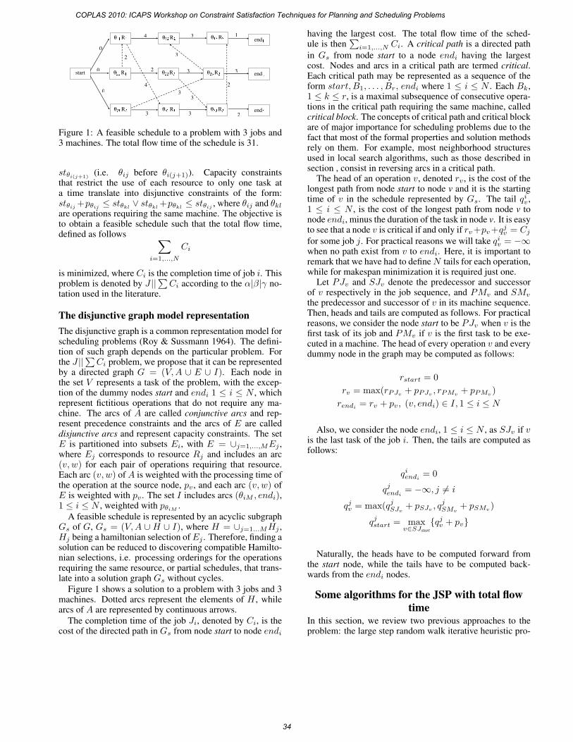
Figure 1: A feasible schedule to a problem with 3 jobs and3 machines. The total flow time of the schedule is 31.

stθi(j+1) (i.e. θij before θi(j+1)). Capacity constraintsthat restrict the use of each resource to only one task ata time translate into disjunctive constraints of the form:stθij +pθij ≤ stθkl

∨ stθkl+pθkl

≤ stθij , where θij and θklare operations requiring the same machine. The objective isto obtain a feasible schedule such that the total flow time,defined as follows ∑

i=1,...,N

Ci

is minimized, where Ci is the completion time of job i. Thisproblem is denoted by J ||∑Ci according to the α|β|γ no-tation used in the literature.

The disjunctive graph model representationThe disjunctive graph is a common representation model forscheduling problems (Roy & Sussmann 1964). The defini-tion of such graph depends on the particular problem. Forthe J ||∑Ci problem, we propose that it can be representedby a directed graph G = (V,A ∪ E ∪ I). Each node inthe set V represents a task of the problem, with the excep-tion of the dummy nodes start and endi 1 ≤ i ≤ N , whichrepresent fictitious operations that do not require any ma-chine. The arcs of A are called conjunctive arcs and rep-resent precedence constraints and the arcs of E are calleddisjunctive arcs and represent capacity constraints. The setE is partitioned into subsets Ei, with E = ∪j=1,...,MEj ,where Ej corresponds to resource Rj and includes an arc(v, w) for each pair of operations requiring that resource.Each arc (v, w) ofA is weighted with the processing time ofthe operation at the source node, pv , and each arc (v, w) ofE is weighted with pv . The set I includes arcs (θiM , endi),1 ≤ i ≤ N , weighted with pθiM .

A feasible schedule is represented by an acyclic subgraphGs of G, Gs = (V,A ∪ H ∪ I), where H = ∪j=1...MHj ,Hj being a hamiltonian selection ofEj . Therefore, finding asolution can be reduced to discovering compatible Hamilto-nian selections, i.e. processing orderings for the operationsrequiring the same resource, or partial schedules, that trans-late into a solution graph Gs without cycles.

Figure 1 shows a solution to a problem with 3 jobs and 3machines. Dotted arcs represent the elements of H , whilearcs of A are represented by continuous arrows.

The completion time of the job Ji, denoted by Ci, is thecost of the directed path in Gs from node start to node endi

having the largest cost. The total flow time of the sched-ule is then

∑i=1,...,N Ci. A critical path is a directed path

in Gs from node start to a node endi having the largestcost. Nodes and arcs in a critical path are termed critical.Each critical path may be represented as a sequence of theform start, B1, . . . , Br, endi where 1 ≤ i ≤ N . Each Bk,1 ≤ k ≤ r, is a maximal subsequence of consecutive opera-tions in the critical path requiring the same machine, calledcritical block. The concepts of critical path and critical blockare of major importance for scheduling problems due to thefact that most of the formal properties and solution methodsrely on them. For example, most neighborhood structuresused in local search algorithms, such as those described insection , consist in reversing arcs in a critical path.

The head of an operation v, denoted rv , is the cost of thelongest path from node start to node v and it is the startingtime of v in the schedule represented by Gs. The tail qiv ,1 ≤ i ≤ N , is the cost of the longest path from node v tonode endi, minus the duration of the task in node v. It is easyto see that a node v is critical if and only if rv+pv+qjv = Cjfor some job j. For practical reasons we will take qiv = −∞when no path exist from v to endi. Here, it is important toremark that we have had to defineN tails for each operation,while for makespan minimization it is required just one.

Let PJv and SJv denote the predecessor and successorof v respectively in the job sequence, and PMv and SMv

the predecessor and successor of v in its machine sequence.Then, heads and tails are computed as follows. For practicalreasons, we consider the node start to be PJv when v is thefirst task of its job and PMv if v is the first task to be exe-cuted in a machine. The head of every operation v and everydummy node in the graph may be computed as follows:

rstart = 0rv = max(rPJv + pPJv , rPMv + pPMv )rendi = rv + pv, (v, endi) ∈ I, 1 ≤ i ≤ N

Also, we consider the node endi, 1 ≤ i ≤ N , as SJv if vis the last task of the job i. Then, the tails are computed asfollows:

qiendi= 0

qjendi= −∞, j �= i

qjv = max(qjSJv+ pSJv , q

jSMv

+ pSMv )

qjstart = maxv∈SJstart

{qjv + pv}

Naturally, the heads have to be computed forward fromthe start node, while the tails have to be computed back-wards from the endi nodes.

Some algorithms for the JSP with total flowtime

In this section, we review two previous approaches to theproblem: the large step random walk iterative heuristic pro-


34

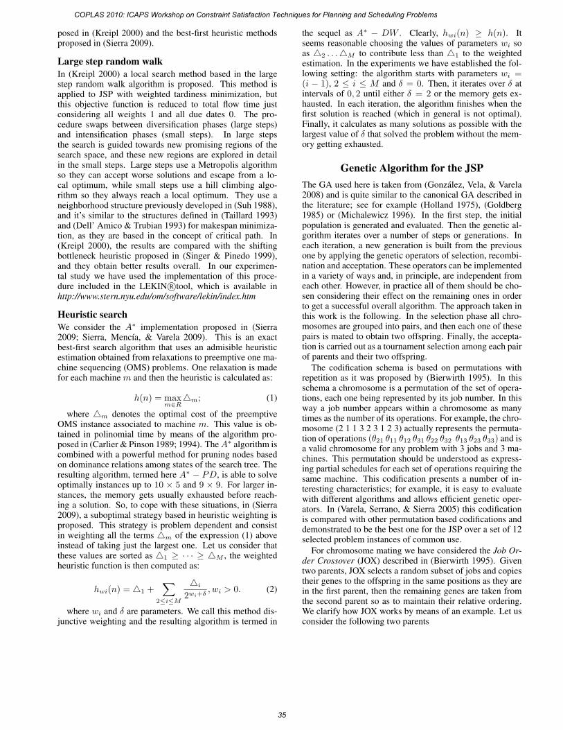
posed in (Kreipl 2000) and the best-first heuristic methodsproposed in (Sierra 2009).

Large step random walkIn (Kreipl 2000) a local search method based in the largestep random walk algorithm is proposed. This method isapplied to JSP with weighted tardiness minimization, butthis objective function is reduced to total flow time justconsidering all weights 1 and all due dates 0. The pro-cedure swaps between diversification phases (large steps)and intensification phases (small steps). In large stepsthe search is guided towards new promising regions of thesearch space, and these new regions are explored in detailin the small steps. Large steps use a Metropolis algorithmso they can accept worse solutions and escape from a lo-cal optimum, while small steps use a hill climbing algo-rithm so they always reach a local optimum. They use aneighborhood structure previously developed in (Suh 1988),and it’s similar to the structures defined in (Taillard 1993)and (Dell’ Amico & Trubian 1993) for makespan minimiza-tion, as they are based in the concept of critical path. In(Kreipl 2000), the results are compared with the shiftingbottleneck heuristic proposed in (Singer & Pinedo 1999),and they obtain better results overall. In our experimen-tal study we have used the implementation of this proce-dure included in the LEKIN R©tool, which is available inhttp://www.stern.nyu.edu/om/software/lekin/index.htm

Heuristic searchWe consider the A∗ implementation proposed in (Sierra2009; Sierra, Mencıa, & Varela 2009). This is an exactbest-first search algorithm that uses an admisible heuristicestimation obtained from relaxations to preemptive one ma-chine sequencing (OMS) problems. One relaxation is madefor each machine m and then the heuristic is calculated as:

h(n) = maxm∈R

�m; (1)

where �m denotes the optimal cost of the preemptiveOMS instance associated to machine m. This value is ob-tained in polinomial time by means of the algorithm pro-posed in (Carlier & Pinson 1989; 1994). TheA∗ algorithm iscombined with a powerful method for pruning nodes basedon dominance relations among states of the search tree. Theresulting algorithm, termed here A∗ − PD, is able to solveoptimally instances up to 10 × 5 and 9 × 9. For larger in-stances, the memory gets usually exhausted before reach-ing a solution. So, to cope with these situations, in (Sierra2009), a suboptimal strategy based in heuristic weighting isproposed. This strategy is problem dependent and consistin weighting all the terms �m of the expression (1) aboveinstead of taking just the largest one. Let us consider thatthese values are sorted as �1 ≥ · · · ≥ �M , the weightedheuristic function is then computed as:

hwi(n) = �1 +∑

2≤i≤M

�i

2wi+δ, wi > 0. (2)

where wi and δ are parameters. We call this method dis-junctive weighting and the resulting algorithm is termed in

the sequel as A∗ − DW . Clearly, hwi(n) ≥ h(n). Itseems reasonable choosing the values of parameters wi soas �2 . . .�M to contribute less than �1 to the weightedestimation. In the experiments we have established the fol-lowing setting: the algorithm starts with parameters wi =(i − 1), 2 ≤ i ≤ M and δ = 0. Then, it iterates over δ atintervals of 0, 2 until either δ = 2 or the memory gets ex-hausted. In each iteration, the algorithm finishes when thefirst solution is reached (which in general is not optimal).Finally, it calculates as many solutions as possible with thelargest value of δ that solved the problem without the mem-ory getting exhausted.

Genetic Algorithm for the JSPThe GA used here is taken from (Gonzalez, Vela, & Varela2008) and is quite similar to the canonical GA described inthe literature; see for example (Holland 1975), (Goldberg1985) or (Michalewicz 1996). In the first step, the initialpopulation is generated and evaluated. Then the genetic al-gorithm iterates over a number of steps or generations. Ineach iteration, a new generation is built from the previousone by applying the genetic operators of selection, recombi-nation and acceptation. These operators can be implementedin a variety of ways and, in principle, are independent fromeach other. However, in practice all of them should be cho-sen considering their effect on the remaining ones in orderto get a successful overall algorithm. The approach taken inthis work is the following. In the selection phase all chro-mosomes are grouped into pairs, and then each one of thesepairs is mated to obtain two offspring. Finally, the accepta-tion is carried out as a tournament selection among each pairof parents and their two offspring.

The codification schema is based on permutations withrepetition as it was proposed by (Bierwirth 1995). In thisschema a chromosome is a permutation of the set of opera-tions, each one being represented by its job number. In thisway a job number appears within a chromosome as manytimes as the number of its operations. For example, the chro-mosome (2 1 1 3 2 3 1 2 3) actually represents the permuta-tion of operations (θ21 θ11 θ12 θ31 θ22 θ32 θ13 θ23 θ33) and isa valid chromosome for any problem with 3 jobs and 3 ma-chines. This permutation should be understood as express-ing partial schedules for each set of operations requiring thesame machine. This codification presents a number of in-teresting characteristics; for example, it is easy to evaluatewith different algorithms and allows efficient genetic oper-ators. In (Varela, Serrano, & Sierra 2005) this codificationis compared with other permutation based codifications anddemonstrated to be the best one for the JSP over a set of 12selected problem instances of common use.

For chromosome mating we have considered the Job Or-der Crossover (JOX) described in (Bierwirth 1995). Giventwo parents, JOX selects a random subset of jobs and copiestheir genes to the offspring in the same positions as they arein the first parent, then the remaining genes are taken fromthe second parent so as to maintain their relative ordering.We clarify how JOX works by means of an example. Let usconsider the following two parents


35

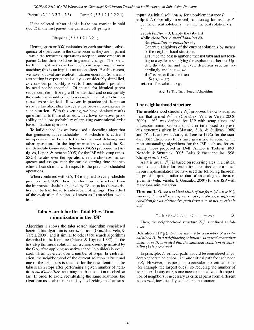
Parent1 (2 1 1 3 2 3 1 2 3) Parent2 (3 3 1 2 1 3 2 2 1)

If the selected subset of jobs is the one marked in bold(job 2) in the first parent, the generated offspring is

Offspring (2 3 3 1 2 1 3 2 1).

Hence, operator JOX maintains for each machine a subse-quence of operations in the same order as they are in parent1 while the remaining operations keep the same order as inparent 2, but their positions in general change. The opera-tor JOX might swap any two operations requiring the samemachine; this is an implicit mutation effect. For this reason,we have not used any explicit mutation operator. So, param-eter setting in experimental study is considerably simplified,as crossover probability is set to 1 and mutation probabil-ity need not be specified. Of course, for identical parentsequences, the offspring will be identical and consequentlythe evolution would come to a complete halt if all chromo-somes were identical. However, in practice this is not anissue as the algorithm always stops before convergence tosuch situation. With this setting, we have obtained resultsquite similar to those obtained with a lower crossover prob-ability and a low probability of applying conventional orderbased mutation operators.

To build schedules we have used a decoding algorithmthat generates active schedules. A schedule is active ifno operation can be started earlier without delaying anyother operation. In the implementation we used the Se-rial Schedule Generation Schema (SSGS) proposed in (Ar-tigues, Lopez, & Ayache 2005) for the JSP with setup times.SSGS iterates over the operations in the chromosome se-quence and assigns each the earliest starting time that sat-isfies all constraints with respect to the previous scheduledoperations.

When combined with GA, TS is applied to every scheduleproduced by SSGS. Then, the chromosome is rebuilt fromthe improved schedule obtained by TS, so as its characteris-tics can be transferred to subsequent offsprings. This effectof the evaluation function is known as Lamarckian evolu-tion.

Tabu Search for the Total Flow Timeminimization in the JSP

Algorithm 1 shows the tabu search algorithm consideredherein. This algorithm is borrowed from (Gonzalez, Vela, &Varela 2009), and it similar to other tabu search algorithmsdescribed in the literature (Glover & Laguna 1997). In thefirst step the initial solution (i.e. a chromosome generated bythe GA, after applying an active schedule builder) is evalu-ated. Then, it iterates over a number of steps. In each iter-ation, the neighborhood of the current solution is built andone of the neighbors is selected for the next iteration. Thetabu search stops after performing a given number of itera-tions maxGlobalIter, returning the best solution reached sofar. In order to avoid reevaluating the same solutions, thealgorithm uses tabu tenure and cycle checking mechanisms.

input An initial solution s0 for a problem instance Poutput A (hopefully improved) solution sB for instance P

Set the current solution s = s0 and the best solution sB =s;Set globalIter = 0, Empty the tabu list;while globalIter < maxGlobalIter do

Set globalIter = globalIter+1;Generate neighbors of the current solution s by meansof the neighborhood structure;Let s* be the best neighbor either not tabu and not lead-ing to a cycle or satisfying the aspiration criterion. Up-date the tabu list and the cycle detection structure ac-cordingly and let s = s∗;if s* is better than sB then

Set sB = s*;return The solution sB ;

Alg. 1: The Tabu Search Algorithm

The neighborhood structureThe neighborhood structure NS

F proposed below is adapted

from that termed NS in (Gonzalez, Vela, & Varela 2008;2009). NS was defined for JSP with setup times andmakespan minimization and it is in turn based on previ-ous structures given in (Matsuo, Suh, & Sullivan 1988)and (Van Laarhoven, Aarts, & Lenstra 1992) for the stan-dard JSP. These structures have given rise to some of themost outstanding algorithms for the JSP such as, for ex-ample, those proposed in (Dell’ Amico & Trubian 1993;Nowicki & Smutnicki 2005; Balas & Vazacopoulos 1998;Zhang et al. 2008).

As it is usual, NSF is based on reversing arcs in a critical

path, so a condition for feasibility is required after a move.In our implementation we have used the following theorem.Its proof is quite similar to that of an analogous theoremgiven in (Vela, Varela, & Gonzalez 2009) for the JSP withmakespan minimization.

Theorem 1. Given a critical block of the form (b′ v b w b′′),where b, b′ and b′′ are sequences of operations, a sufficientcondition for an alternative path from v to w not to exist isthat

∀u ∈ {v} ∪ b, rPJw < rSJu + pSJu (3)

Then, the neighborhood structure NSF is defined as fol-

lows.

Definition 1 (NSF ). Let operation v be a member of a criti-

cal blockB. In a neighboring solution v is moved to anotherposition in B, provided that the sufficient condition of feasi-bility (3) is preserved.

In principle, N critical paths should be considered in or-der to generate neighbors, i.e. one critical path for each nodeendi. However, it is possible to consider less critical paths(for example the largest ones), so reducing the number ofneighbors. In any case, some mechanism to avoid the repeti-tion of neighbors is necessary as critical paths from differentnodes endi have usually some parts in common.


36

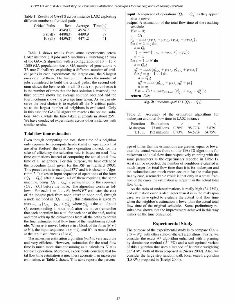
Table 1: Results of GA+TS across instance LA02 exploitingdifferent numbers of critical paths

Critical Paths Best Average Time(s.)1 4545(1) 4574.7 32

5 (half) 4480(3) 4490.9 3710 (all) 4459(2) 4471.2 41

Table 1 shows results from some experiments acrossLA02 instance (10 jobs and 5 machines), launching 15 runsof the GA+TS algorithm with a configuration of 10 × 15 ×1500 (GA population size × GA number of generations ×TS maxGlobalIter), exploiting a different number of criti-cal paths in each experiment: the largest one, the 5 largestones or all of them. The first column shows the number ofjobs considered to build the critical paths, the second col-umn shows the best result in all 15 runs (in parentheses itis the number of times that the best solution is reached), thethird column shows the average solution obtained and thefourth column shows the average time taken. As we can ob-serve the best choice is to exploit all the N critical paths,so as the largest number of neighbors is evaluated. Onlyin this case the GA+TS algorithm reaches the optimal solu-tion (4459), while the time taken augments in about 25%.We have conducted experiments across other instances withsimilar results.

Total flow time estimationEven though computing the total flow time of a neighboronly requires to recompute heads (tails) of operations thatare after (before) the first (last) operation moved, for thesake of efficiency the selection rule is based on total flowtime estimations instead of computing the actual total flowtime of all neighbors. For this purpose, we have extendedthe procedure lpath given for the JSP in (Taillard 1993).This procedure is termed lpathTFT and it is shown in Algo-rithm 2. It takes an input sequence of operations of the form(Q1 . . . Qq) after a move, all of them requiring the samemachine, being (Q1 . . . Qq) a permutation of the sequence(O1 . . . Oq) before the move. The algorithm works as fol-lows: For each i = 1 . . . N , lpathTFT estimates the costof the longest path from node start to node endi througha node included in (Q1 . . . Qq), this estimation is given by

maxj=1...q {r′Qj+ pQj

+ q′iQj, where q′iQj

is the tail of node

Qj corresponding to node endi after the move (rememberthat each operation has a tail for each one of the endi nodes)and then adds up the estimations from all the paths to obtainthe final estimated total flow time of the neighboring sched-ule. When w is moved before v in a block of the form (b′ v bw b′′), the input sequence is (w v b), and if v is moved afterw the input sequence is (b w v).

The makespan estimation algorithm lpath is very accurateand very efficient. However, estimation for the total flowtime is much more time consuming as it calculates N tailsfor each operation. Moreover, experiments conclude that to-tal flow time estimation is much less accurate than makespanestimation, as Table 2 shows. This table reports the percent-

input A sequence of operations (Q1 . . . Qq) as they appearafter a move

output A estimation of the total flow time of the resultingscheduleEst = 0;a = Q1;r′a = max {rPJa + pPJa , rPMa + pPMa};for i = 2 to q dob = Qi;r′b = max {rPJb

+ pPJb, r′a + pa};

a = b;for i = 1 to N dob = Qq;q′ib = max {qiSJb

+ pSJb, qiSMb

+ pSMb};

for j = q − 1 to 1 doa = Qj ;q′ia = max {qiSJa

+ pSJa, q′ib + pb};

b = a;Est = Est+ maxj=1...q {r′Qj

+ pQj+ q′iQj

};

return Est;

Alg. 2: Procedure lpathTFT (Q1 . . . Qq)

Table 2: Accuracy of the estimation algorithms formakespan and total flow time in LA02 instance

Function Estimations > = <Makespan 77 millions 0.36% 95.77% 3.87%

T. F. T. 192 millions 0.73% 64.52% 34.75%

age of times that the estimations are greater, equal or lowerthan the actual values from similar GA+TS algorithms formakespan and total flow time respectively (running with thesame parameters as the experiments reported in Table 1).As it can be expected, the number of neighbors evaluated ismuch larger for total flow time than it is for makespan andthe estimations are much more accurate for the makespan.In any case, a remarkable result is that only in a small frac-tion of the cases the estimation is larger than the actual totalflow time.

As the ratio of underestimations is really high (34.75%),and estimation error is also larger than it is in the makespancase, we have opted to evaluate the actual total flow timewhen the neighbor’s estimation is lower than the actual totalflow time of the original schedule. Some preliminary re-sults have shown that the improvement achieved in this waymakes up the time consumed.

Experimental StudyThe purpose of the experimental study is to compare GA+TS −NS

F with other state-of-the-art algorithms. Firstly, weconsider the exact A* algorithm enhanced with a pruningby dominance method (A∗-PD) and a sub-optimal variantof this algorithm that uses a method of heuristic weighting(A∗-DW), both of them proposed in (Sierra 2009). Also, weconsider the large step random walk local search algorithm(LSRW) proposed in (Kreipl 2000).


37

We have conducted two series of experiments on standardbenchmarks taken from the OR-library. In the first one, weexperimented across a set of instances (sizes 10×5, 8×8 and9×9) proposed in (Sierra 2009), that are optimally solved byA∗-PD. The reduced 8×8 and 9×9 instances are built fromoriginal 10 × 10 instances removing the last jobs and thelast machines. In the second series of experiments we usedlarger instances (sizes 15×5, 20×5 and 10×10) that can notbe optimally solved by A∗-PD. In all these experiments, wehave to be aware of the differences in the target machinesand then in the time taken. The versions of A∗ have beenrun on Ubuntu V8,04 on Intel Core 2 Duo at 2,13GHz with7,6Gb of RAM, LSRW has been run on Windows XP onIntel Core 2 Duo at 2,13GHz with 3Gb of RAM and GA +TS−NS

F has been run on Windows XP on Intel Core 2 Duoat 2.66GHz with 2Gb of RAM.

Table 3 shows results from the first experiments. In thiscase A∗-PD reach the optimal solutions for all instances.LSRW and GA + TS − NS

F were run 20 times for eachinstance and the best and average values of all 20 solutionsare reported. The GA+ TS −NS

F parameters (GA popula-tion size × GA number of generations × TS maxGlobalIter)were (50 × 70 × 150) for both 10 × 5 and 9 × 9 instances,and (30 × 40 × 120) for 8 × 8 instances. With these val-ues the algorithm converges properly and the time taken isnot larger than that of the other two algorithms (taking intoaccount the target machines).

As we can observe, GA + TS − NSF is able to reach the

optimum solution in most of the trials: it reached the opti-mal solution in 747 out of the 820 runs for all 41 instances(91.1%), and has reached at least once the optimal solutionfor 40 of the 41 instances. The exception is the instanceORB08(9 × 9) where A∗-PD takes the largest time amongthe 9×9 instances. LSRW fails to reach the optimal solutionin 6 of the 41 instances.

In the second series of experiments we compare A∗-DW,LSRW and GA + TS − NS

F on the set of instances LA06-10 (15 × 5), LA11-15 (20 × 5) and LA15-20 (10 × 10).None of these instances can be optimally solved by A∗-PDbefore the memory getting exhausted, so we do not knowtheir optimal solutions. In these experiments theGA+TS−NSF parameters were (50 × 70 × 150) for all 15 instances,

run.

Table 4 shows the results from these experiments. Here,the time reported for A∗-DW corresponds to the number oftrials that are required to adjust the parameter δ to its bestvalue and one more to obtain all possible solutions withthis parameter, the time taken until the memory getting ex-hausted or the whole search space is explored is accumulatedfor all trials. For LWRS and GA+TS−NS

F the time is theaverage time of 20 trials.

As we can observe, in average GA + TS −NSF is better

than LSRW in 12 instances and it is worse in 3; and the bestvalue of GA+ TS −NS

F is better than that of LSRW in 11

and equal in 4. Compared to A∗-DW, GA+ TS −NSF is in

average better in 7 cases, equal in 5 and worse in 3, and thebest value of GA+ TS −NS

F is better in 8 cases and equalin the remaining ones.

ConclusionsWe have considered the job shop scheduling problem, wherethe objective is to minimize the total flow time. We haveproposed a disjunctive graph representation for this problemand used it to define a specific neighborhood structure forthe total flow time. The neighborhood structure has thenbeen used in a tabu search algorithm, which is embeddedin a genetic algorithm framework. We have also defined amethod for estimating the total flow time of the neighbors,and demonstrated that estimating this objective function ismuch more difficult than estimating other classic objectivefunctions such as the makespan.

We have reported results from an experimental studyacross some conventional benchmarks and compared theproposed GA+ TS −NS

F algorithm with some representa-tive state-of-the-art methods: the A∗ algorithm with a prun-ing by dominance method (A∗-PD) and the A∗-DW, bothproposed in (Sierra 2009), and the large step random walkalgorithm (LSRW) proposed in (Kreipl 2000). The resultsshow that the proposed approach is competitive with thesestate-of-the-art methods.

As future work we plan to extend our approach to con-front other variants or extensions of this problem. We wouldlike to consider the weighted tardiness as objective function,which is very interesting too in real life applications, and it isa generalization of total flow time. It would also be interest-ing to tackle multiobjective problems. Finally, our approachmay also be applied to more general frameworks than JSP,such as resource-constrained scheduling with setup times.

AcknowledgmentsThis work is supported by MEC-FEDER Grant TIN2007-67466-C02-01 and FICYT grant BP07-109.

ReferencesArtigues, C.; Lopez, P.; and Ayache, P. 2005. Sched-ule generation schemes for the job shop problem withsequence-dependent setup times: Dominance propertiesand computational analysis. Annals of Operations Re-search 138:21–52.

Balas, E., and Vazacopoulos, A. 1998. Guided local searchwith shifting bottleneck fo job shop scheduling. Manage-ment Science 44(2):262–275.

Bierwirth, C. 1995. A generalized permutation approach tojobshop scheduling with genetic algorithms. OR Spectrum17:87–92.

Brucker, P. 2004. Scheduling Algorithms. Springer, 4thedition.

Carlier, J., and Pinson, E. 1989. An algorithm for solvingthe job-shop problem. Management Science 35(2):164–176.

Carlier, J., and Pinson, E. 1994. Adjustment of heads andtails for the job-shop problem. European Journal of Oper-ational Research 78:146–161.

Dell’ Amico, M., and Trubian, M. 1993. Applying tabusearch to the job-shop scheduling problem. Annals of Op-erational Research 41:231–252.


38

Glover, F., and Laguna, M. 1997. Tabu Search. KluwerAcademic Publishers.

Goldberg, D. 1985. Genetic algorithms in search. Opti-mization and machine learning. Addison-Wesley.

Gonzalez, M. A.; Vela, C. R.; and Varela, R. 2008. Anew hybrid genetic algorithm for the job shop schedulingproblem with setup times. In Proceedings of the Eigh-teenth International Conference on Automated Planningand Scheduling (ICAPS-2008). Sidney: AAAI Press.

Gonzalez, M. A.; Vela, C. R.; and Varela, R. 2009. Ge-netic algorithm combined with tabu search for the job shopscheduling problem with setup times. In IWINAC 2009:Methods and Models in Artificial and Natural Computa-tion, 265–274. LNCS-5601, Springer.

Holland, J. H. 1975. Adaptation in Natural and ArtificialSystems: An Introductory Analysis with Applications to Bi-ology, Control and Artificial Intelligence. The Universityof Michigan Press.

Kreipl, S. 2000. A large step random walk for minimizingtotal weighted tardiness in a job shop. Journal of Schedul-ing 3:125–138.

Matsuo, H.; Suh, C.; and Sullivan, R. 1988. A controlledsearch simulated annealing method for the general jobshopscheduling problem. Working paper 03-44-88, GraduateSchool of Business, University of Texas.

Michalewicz, Z. 1996. Genetic Algorithms + Data Struc-tures = Evolution Programs. Springer, third, revised andextended edition.

Nowicki, E., and Smutnicki, C. 2005. An advanced tabusearch algorithm for the job shop problem. Journal ofScheduling 8:145–159.

Roy, B., and Sussmann, B. 1964. Les problemesd’ordonnancement avec constraintes disjonctives. Note d.s.no. 9 bis, d6c, SEMA, Matrouge, Paris.

Sierra, M., and Varela, R. 2007. Pruning by dominancein best-first search. In Proceedings of CAEPIA’2007, vol-ume 2, 289–298.

Sierra, M., and Varela, R. 2008a. A new admissible heuris-tic for the job shop scheduling problem with total flowtime. ICAPS-2008. Workshop on Constraint SatisfactionTechniques for Planning and Scheduling. Sidney.

Sierra, M., and Varela, R. 2008b. Pruning by dominance inbest-first search for the job shop scheduling problem withtotal flow time. Journal of Intelligent Manufacturing, DOI10.1007/s10845-008-0167-4 1:1–2.

Sierra, M. R., and Varela, R. 2010. Best-first search andpruning by dominance for the job shop scheduling problemwith total flow time. Journal of Intelligent Manufacturing21(1):111–119.

Sierra, M. R.; Mencıa, C.; and Varela, R. 2009. Weight-ing disjunctive heuristics for scheduling problems withsummation cost functions. In Proceedings of Work-shop on Planning, Scheduling and Constraint Satisfaction,CAEPIA’2009.

Sierra, M. R. 2009. Metodos de Poda por Dominan-cia en Busqueda Heurıstica. Aplicaciones a Problemas de

Scheduling. Ph.D. Dissertation, Universidad de Oviedo,Spain.

Singer, M., and Pinedo, M. 1999. A shifting bottleneckheuristic for minimizing the total weighted tardiness in ajob shop. Naval Research Logistics 46(1):1–17.

Suh, C. 1988. Controlled search simulated annealingfor job shop scheduling. Ph.D. Dissertation, University ofTexas.

Taillard, E. 1993. Benchmarks for basic scheduling prob-lems. European Journal of Operational Research 64:278–285.

Van Laarhoven, P.; Aarts, E.; and Lenstra, K. 1992. Jobshop scheduling by simulated annealing. Operations Re-search 40:113–125.

Varela, R.; Serrano, D.; and Sierra, M. 2005. New cod-ification schemas for scheduling with genetic algorithms.Proceedings of IWINAC 2005. Lecture Notes in ComputerScience 3562:11–20.

Vela, C. R.; Varela, R.; and Gonzalez, M. A. 2009. Localsearch and genetic algorithm for the job shop schedulingproblem with sequence dependent setup times. Journal ofHeuristics DOI 10.1007/s10732-008-9094-y.

Zhang, C. Y.; Li, P.; Rao, Y.; and Guan, Z. 2008. A veryfast TS/SA algorithm for the job shop scheduling problem.Computers and Operations Research 35:282–294.


39

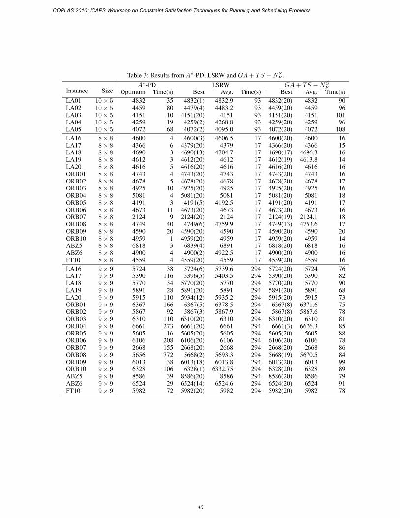
Table 3: Results from A∗-PD, LSRW and GA+ TS −NSF .

Instance SizeA∗-PD LSRW GA+ TS −NS

FOptimum Time(s) Best Avg. Time(s) Best Avg. Time(s)

LA01 10 × 5 4832 35 4832(1) 4832.9 93 4832(20) 4832 90LA02 10 × 5 4459 80 4479(4) 4483.2 93 4459(20) 4459 96LA03 10 × 5 4151 10 4151(20) 4151 93 4151(20) 4151 101LA04 10 × 5 4259 19 4259(2) 4268.8 93 4259(20) 4259 96LA05 10 × 5 4072 68 4072(2) 4095.0 93 4072(20) 4072 108

LA16 8 × 8 4600 4 4600(3) 4606.5 17 4600(20) 4600 16LA17 8 × 8 4366 6 4379(20) 4379 17 4366(20) 4366 15LA18 8 × 8 4690 3 4690(13) 4704.7 17 4690(17) 4696.3 16LA19 8 × 8 4612 3 4612(20) 4612 17 4612(19) 4613.8 14LA20 8 × 8 4616 5 4616(20) 4616 17 4616(20) 4616 16ORB01 8 × 8 4743 4 4743(20) 4743 17 4743(20) 4743 16ORB02 8 × 8 4678 5 4678(20) 4678 17 4678(20) 4678 17ORB03 8 × 8 4925 10 4925(20) 4925 17 4925(20) 4925 16ORB04 8 × 8 5081 4 5081(20) 5081 17 5081(20) 5081 18ORB05 8 × 8 4191 3 4191(5) 4192.5 17 4191(20) 4191 17ORB06 8 × 8 4673 11 4673(20) 4673 17 4673(20) 4673 16ORB07 8 × 8 2124 9 2124(20) 2124 17 2124(19) 2124.1 18ORB08 8 × 8 4749 40 4749(6) 4759.9 17 4749(13) 4753.6 17ORB09 8 × 8 4590 20 4590(20) 4590 17 4590(20) 4590 20ORB10 8 × 8 4959 1 4959(20) 4959 17 4959(20) 4959 14ABZ5 8 × 8 6818 3 6839(4) 6891 17 6818(20) 6818 16ABZ6 8 × 8 4900 4 4900(2) 4922.5 17 4900(20) 4900 16FT10 8 × 8 4559 4 4559(20) 4559 17 4559(20) 4559 16

LA16 9 × 9 5724 38 5724(6) 5739.6 294 5724(20) 5724 76LA17 9 × 9 5390 116 5396(5) 5403.5 294 5390(20) 5390 82LA18 9 × 9 5770 34 5770(20) 5770 294 5770(20) 5770 90LA19 9 × 9 5891 28 5891(20) 5891 294 5891(20) 5891 68LA20 9 × 9 5915 110 5934(12) 5935.2 294 5915(20) 5915 73ORB01 9 × 9 6367 166 6367(5) 6378.5 294 6367(8) 6371.6 75ORB02 9 × 9 5867 92 5867(3) 5867.9 294 5867(8) 5867.6 78ORB03 9 × 9 6310 110 6310(20) 6310 294 6310(20) 6310 81ORB04 9 × 9 6661 273 6661(20) 6661 294 6661(3) 6676.3 85ORB05 9 × 9 5605 16 5605(20) 5605 294 5605(20) 5605 88ORB06 9 × 9 6106 208 6106(20) 6106 294 6106(20) 6106 78ORB07 9 × 9 2668 155 2668(20) 2668 294 2668(20) 2668 86ORB08 9 × 9 5656 772 5668(2) 5693.3 294 5668(19) 5670.5 84ORB09 9 × 9 6013 38 6013(18) 6013.8 294 6013(20) 6013 99ORB10 9 × 9 6328 106 6328(1) 6332.75 294 6328(20) 6328 89ABZ5 9 × 9 8586 39 8586(20) 8586 294 8586(20) 8586 79ABZ6 9 × 9 6524 29 6524(14) 6524.6 294 6524(20) 6524 91FT10 9 × 9 5982 72 5982(20) 5982 294 5982(20) 5982 78


40

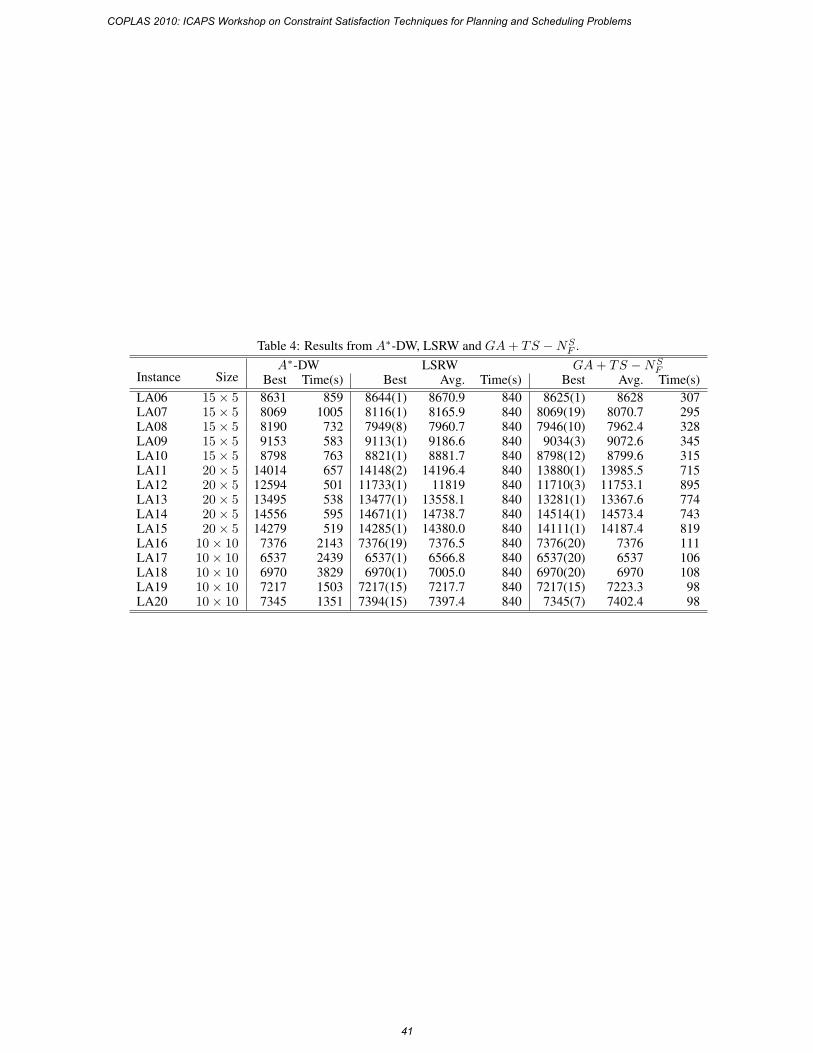
Table 4: Results from A∗-DW, LSRW and GA+ TS −NSF .

Instance SizeA∗-DW LSRW GA+ TS −NS

FBest Time(s) Best Avg. Time(s) Best Avg. Time(s)

LA06 15 × 5 8631 859 8644(1) 8670.9 840 8625(1) 8628 307LA07 15 × 5 8069 1005 8116(1) 8165.9 840 8069(19) 8070.7 295LA08 15 × 5 8190 732 7949(8) 7960.7 840 7946(10) 7962.4 328LA09 15 × 5 9153 583 9113(1) 9186.6 840 9034(3) 9072.6 345LA10 15 × 5 8798 763 8821(1) 8881.7 840 8798(12) 8799.6 315LA11 20 × 5 14014 657 14148(2) 14196.4 840 13880(1) 13985.5 715LA12 20 × 5 12594 501 11733(1) 11819 840 11710(3) 11753.1 895LA13 20 × 5 13495 538 13477(1) 13558.1 840 13281(1) 13367.6 774LA14 20 × 5 14556 595 14671(1) 14738.7 840 14514(1) 14573.4 743LA15 20 × 5 14279 519 14285(1) 14380.0 840 14111(1) 14187.4 819LA16 10 × 10 7376 2143 7376(19) 7376.5 840 7376(20) 7376 111LA17 10 × 10 6537 2439 6537(1) 6566.8 840 6537(20) 6537 106LA18 10 × 10 6970 3829 6970(1) 7005.0 840 6970(20) 6970 108LA19 10 × 10 7217 1503 7217(15) 7217.7 840 7217(15) 7223.3 98LA20 10 × 10 7345 1351 7394(15) 7397.4 840 7345(7) 7402.4 98


41

Casting Project Scheduling with Time Windows as a DTP

Angelo Oddi, Riccardo Rasconi and Amedeo Cesta

ISTC-CNR, Italian National Research Council, Italy

AbstractThis paper extends existing work on constraint-basedscheduling for solving complex Resource ConstrainedProject Scheduling Problems. The main result of the paperis the reduction of the RCPSP/max problem to a DisjunctiveTemporal Problem that allow customization of specific prop-erties within a backtracking search procedure for makespanoptimization where decision variables are Minimal CriticalSets (MCSs). In particular an algorithm is proposed whosebranching strategy is able to deduce new constraints whichexplicitly represent infeasible or useless search paths, suchadditional information allows early pruning of alternativesand strongly improves the efficiency of the overall search pro-cedure. The paper includes an experimental evaluation on aset of standard, quite challenging, benchmark problems giv-ing an empirical validation of the effectiveness of the pro-posed ideas.

IntroductionIn this paper we present a constraint-based procedureto solve instances of the Resource Constrained ProjectScheduling Problem with Generalized Precedence Relations(RCPSP/max). This problem derives from a project man-agement environment in which activities represent steps thatmust be performed to achieve completion of the project andare subject to partial order constraints that reflect dependen-cies on project progression. In particular, a time windowconstraint is imposed between a generic pair of activitieswhich bounds the difference of the start times of the ac-tivities to be included in a interval of possible values. Thepresence of this kind of constraint makes the problem hardto solve; as demonstrated in (Bartusch, Mohring, and Ra-dermacher 1988), both the optimization and the feasibilityversions of the problem are NP-hard.

This paper draws on ideas from two existing researchlines: (a) contraint-based resource-constrained scheduling(Cesta, Oddi, and Smith 1998; 2002; Laborie 2005) and(b) disjunctive temporal reasoning (Oddi and Cesta 2000;Armando, Castellini, and Giunchiglia 1999; Dechter, Meiri,and Pearl 1991; Stergiou and Koubarakis 2000; Tsamardi-nos and Pollack 2003) In particular, we elaborate from


a basic backtracking search procedure for makespan opti-mization where decision variables are Minimal Critical Sets(MCSs). The algorithm proposes a new branching strat-egy able to deduce new constraints which explicitly repre-sent infeasible or useless search paths; such additional in-formation allows early pruning of alternatives and stronglyimproves the efficiency of the overall search procedure.The proposed procedure iteratively selects decision vari-ables (MCSs) which represent minimal sets of activities re-quiring more of the resource capacity. Given the minimalityof the conflicts (each proper subset is not a resource conflict)a capacity violation is resolved by posting a single prece-dence constraint between any two activities of the MCS.To solve the RCPSP/max problem, we repeatedly apply thiscore CSP by adding/retracting precedence constraint alonga systematic backtracking procedure which stops when ei-ther an optimal solution is found or another stop condition ismet.

The guiding idea of the current work is based on theobservation that a single MCS = {a1, a2, . . . , ak} rep-resents disjunction of literals each representing a simpletemporal problem among the start/end times of the activ-ities ai ∈ MCS of the form start(aj) − end(ai) ≥ 0(start(ai)−end(aj) ≥ 0). A solution of the problem is a setof precedence constraints which induce an ordering of theproblem activities where all the MCSs are explicitly or im-plicitly solved. In other words, a RCPSP/max can be seen asa conjunction of disjuntive temporal formulas correspondingto MCSs of the form x1 − y1 ≤ r1 ∨ x2 − y2 ≤ r2 ∨ . . . ∨xk − yk ≤ rk. Such problem is known as the DisjunctiveTemporal Problem (DTP) (Stergiou and Koubarakis 1998;2000). Given the reduction of RCPSP/max to DTP, manyof the techniques developed for solving DTP instances canbe reused within MCS-based search procedures like thosedescribed in (Cesta, Oddi, and Smith 2002; Laborie 2005).

The paper is organized as follows. It first defines the refer-ence RCPSP/max problem and its representation. The cen-tral section describes the reduction of RCPSP/max to DTPand the core constraint-based search procedure. Then, theperformance of the proposed algorithm is described and themost interesting experimental results explained. Some con-clusions and a discussion on the future work end the paper.


42

The Scheduling ProblemThe Resource Constrained Project Scheduling Problem(RCPSP) has been widely studied in Operations Researchliterature (see (Brucker et al. 1999) for a survey).RCPSP/max is a specific formulation of the basic problemunderlying a number of scheduling applications (Neumannand Schwindt 1997) which is considered particularly diffi-cult, due to the presence of temporal separation constraints(in particular maximum time lags) between project activi-ties.

The RCPSP/max can be formalized as follows:

– a set V of n activities must be executed, where each activ-ity j has a fixed duration dj . Each activity has a start-timeSj and a completion-time Cj that satisfies the constraintSj + dj = Cj .

– a set E of temporal constraints exists between variousactivity pairs 〈i, j〉 of the form Sj − Si ∈ [Tmin

ij , Tmaxij ],

called start-to-start constraints (time lags or generalizedprecedence relations between activities). 1

– a set R of renewable resources are available, where eachresource rk has a integer capacity ck ≥ 1.

– execution of an activity j requires capacity from one ormore resources. For each resource rk the integer rcj,krepresents the required capacity (or size) of activity j.

A schedule S is an assignment of values to the start-timesof all activities in V (S = (S1, . . . , Sn)). A schedule istime-feasible if all temporal constraints are satisfied (all con-straints Sj − Si ∈ [Tmin

ij , Tmaxij ] and Sj + dj = Cj hold).

A schedule is resource-feasible if all resource constraints aresatisfied (let A(S, t) = {i ∈ V |Si ≤ t < Si + di} be the setof activities which are in progress at time t and rk(S, t) =∑

j∈A(S,t) rcj,k the usage of resource rk at that same time;

for each t the constraint rk(S, t) ≤ ck must hold). Aschedule is feasible if both sets of constraints are satis-fied. The RCPSP/max optimization problem, then, is to finda feasible schedule with minimum makespan MK, whereMK(S) = maxi∈V {Ci}.

RCPSP/max as a CSPThere are different ways to formulate the RCPSP/max prob-lem as a Constraint Satisfaction Problem (CSP) (Montanari1974). In particular, see (Cesta, Oddi, and Smith 1998) andmany others, the problem can be treated as the one of es-tablishing precedence constraints between set of activitiesthat require the same resource, so as to eliminate all pos-sible conflicts in resource use. Given a resource r, we callconflict each set of activities requiring r, which can mutuallyoverlap and whose combined resource requirement is morethan the resource capacity c,

1Note that since activity durations are constant values, end-to-end, end-to-start, and start-to-end constraints between activitiescan all be represented in start-to-start form.

Decision variables are called Minimal Critical SetsMCS = {a1, a2, . . . , ak} or forbidden minimal sets (Bar-tusch, Mohring, and Radermacher 1988; Laborie and Ghal-lab 1995). An MCS represents resource conflics of mini-mal size (each subsets is not a resource conflict), which canbe resolved by posting a single precedence constraint be-tween any two of the competing activities in the MCS. InCSP terms, a decision variable is defined for each MCS ={a1, a2, . . . , ak}; which can take as values all the possiblefeasible precedence constraints ai � aj that can be imposedbetween each pair of activities in MCS. It is however wellknown that some of such values are superfluous. In particu-lar, we can use the idea of simplification for a set of prece-dence constraints (or resolvers) for a given decision variable(MCS), as described in (Laborie 2005): the set of resolversRes(MCS) = {pc1, pc2, . . . , pck} of a MCS can be sim-plified so as to remove those resolvers pc× ∈ Res(MCS)for which there exists another resolver pc+ ∈ Res(MCS)such that pc× ⇒ pc+ given the current temporal network.In other words, if a precedence constraint pc× = ai � ajimposed between the pair of activities (ai, aj) induces alsoa precedence constraint pc+ = ai � ak or pc+ = ak � aj ,then pc× can be removed.

To support the search for a consistent assignment to theset of decision variables (MCSs), for any RCPSP/max wedefine the distance graph Gd. The set of nodes V repre-sents time points, that is, the origin point tp0 (the referencepoint of the problem) together with the start and end timepoints, si and ei, of each activity ai. The set of edges Erepresents all the imposed temporal constraints, i.e., prece-dences and durations. All the constraints have the forma ≤ tpj − tpi ≤ b and for each constraint specified inthe RCPSP/max, there are two weighted edges in the graphGd(V,E). The first one is directed from tpi to tpj withweight b and the second one is directed from tpj to tpiwith weight −a. The graph Gd(V,E) corresponds to a Sim-ple Temporal Problem and its consistency can be efficientlydetermined via shortest path computations (see (Dechter,Meiri, and Pearl 1991) for more details on the STP). Thus,a search for a solution of a RCPSP/max instance can pro-ceed by repeatedly adding new precedence constraints intoGd(V,E) and recomputing shortest path lengths to confirmthat Gd(V,E) remains consistent. Given a Simple TemporalProblem, the problem is consistent if and only if no closedpaths with negative length (or negative cycles) are containedin the graph Gd.

Let d(tpi, tpj) (d(tpj , tpi)) designate the shortest pathlength in graph Gd(V,E) from node tpi to node tpj (nodetpj to node tpi), the following constraint −d(tpj , tpi) ≤tpj − tpi ≤ d(tpi, tpj) holds (Dechter, Meiri, and Pearl1991). Hence, the minimal allowed distance betweentpj and tpi is −d(tpj , tpi) and the maximal distance isd(tpi, tpj). Given that di0 is the length of the short-est path on Gd from the time point tpi to the originpoint tp0 and d0i is the length of the shortest path fromthe origin point tp0 to the time point tpi, the interval


43

[lbi, ubi] of time values associated to the generic time vari-able tpi is computed on the graph Gd as the interval[−d(tpi, tp0), d(tp0, tpi)] (see (Dechter, Meiri, and Pearl1991)). In particular, the two set of assignment values Slb ={−d(tp1, tp0),−d(tp2, tp0), . . . ,−d(tpn, tp0)} and Sub ={d(tp0, tp1), d(tp0, tp2), . . . , d(tp0, tpn)} to the variablestpi respectively represent the so-called earliest-time solutionand latest-time solution for the given STP.

We observe that when each MCS is resolved (i.e., at leasta precedence constraint is posted between a pair of activitiesai, aj ∈MCS or it is a consequence of other imposed con-straints) and the corresponding STP is consistent, then wecan easily find a schedule S, i.e, an assignment of valuesto the start-times of all activities in V (S = (S1, . . . , Sn)),which satisfies both all the temporal and the resource con-straints of the problem. In fact, the temporal constraints aresatisfied, because the corresponding STP is consistent, andalso the resource constraints are satisfied. To prove this lastclaim, let us suppose by contradiction that at least one re-source r and an instant of time t exist, such that a set of ac-tivities mutually overlaps and the total requirement is greaterthe resource capacity c. This circumstance would corre-spond to a conflict and would contradict that all the minimalconflicts are indeed removed. Hence, when all the MinimalCritical Sets are removed then all the temporal feasible as-signments to the start times represents a full solution of theproblem. In the following, we will focus on the earliest-timesolution of the problem.

Reducing an RCPSP/max to a DTPThe definition of the RCPSP/max as a CSP problem al-lows a reduction to the Disjunctive Temporal Problem (Ster-giou and Koubarakis 2000). The Disjunctive TemporalProblem (DTP) involves a finite set of temporal variablesx1, y1, x2, y2 . . . xn, yn ranging over the integers 2 and afinite set of constraints C = {c1, c2, . . . cm} of the formx1 − y1 ≤ r1 ∨ x2 − y2 ≤ r2 ∨ . . . ∨ xk − yk ≤ rk,where ri are integer numbers. A DTP is consistent if an as-signment to the variables exists such that in each constraintsci ∈ C at least one disjunct xij − yij ≤ rij is satisfied.One way to check for consistency of a DTP (Oddi and Cesta2000) consists of choosing one disjunct for each constraintci and see if the conjunction of the chosen disjuncts is con-sistent. It is worth observing that this is equivalent to ex-tracting a “particular” STP (the Simple Temporal Problemdefined in (Dechter, Meiri, and Pearl 1991)) from the DTPand checking its consistency. If the STP is not consistentanother one is selected, and so on. Again, as observed in(Oddi and Cesta 2000), a DTP can be represented as a CSPproblem, where each DTP constraint c ∈ C represents a(meta) variable and the set of disjuncts represents variable’sdomain values Dc = {δ1, δ2, . . . δk}. A meta-CSP problemis consistent if exists at least an element S (solution) of the

2In the original definition of the DTP variables ranges overreal values, however we make this restrictive hypothesis becauseRCPSP/max variables range over integers

set D1 ×D2 × . . .×Dm such that the corresponding set ofdisjuncts S = {δ1, δ2, . . . δm} δi ∈ Di is temporally con-sistent. Each value δi ∈ Di represents an inequality of theform xi − yi ≤ ri and a solution S can be represented as alabeled graph Gd(VS , ES) called “distance graph” (Dechter,Meiri, and Pearl 1991). The set of nodes VS coincides withthe set of DTP variables x1, y1, x2, y2 . . . xn, yn and eachdisjunct xi − yi ≤ ri is represented by a direct edge (yi, xi)from yi to xi labeled with ri. Again the graph Gd(VS , ES)represents a Simple Temporal Problem and we can refer tothe properties described in the above section.

A RCPSP/max can be reduced to a DTP as it follows.

– The set of time points of the RCPSP/max, that is, the ori-gin point tp0 (the reference point of the problem) togetherwith the start and end time points, si and ei, of each ac-tivity ai) represent the variables of the DTP.

– For each RCPSP/max constraint of the form a ≤ xi −yi ≤ b (representing duration of activities or start-startwindows constraints), there are two constraints withoutdisjunction, xi − yi ≤ b and yi − xi ≤ −a, added to theset C.

– for each resource rk, each Minimal Critical Set MCS ={a1, a2, . . . , ak} corresponds to a DTP constraint c ={pc1, pc2, . . . , pcm}, such that pck is a feasible prece-dence constraints of the form Si + di ≤ Sj between ageneric pair of activities ai, aj ∈MCS.

On the basis of the above reduction, MCS-based algorithmsfor solving RCPSP/max instances, like the ones describedin (Cesta, Oddi, and Smith 2002; Laborie 2005), can beseen as a meta-CSP based search procedure, a la (Oddi andCesta 2000), which uses the same heuristics and pruningtechniques for the original DTP search procedure. In thenext section we see how to include within a complete MCS-based search algorithm for makespan optimization the ideaof semantic branching as used in (Armando, Castellini, andGiunchiglia 1999).

The MCS-based SearchFigure 1 shows a non-deterministic version of a completeMCS-based procedure (similarly to (Laborie 2005)) whichstarts from a scheduling problem P and an empty solutionS, and basically executes three steps: (a) the current partialsolution is checked for consistency (Step 1) by the functionCheckConsistency. If the partial solution is a complete so-lution (Step 2), that is an earliest-time assignment of val-ues to the start-times of all activities (S = (S1, . . . , Sn)) –which satisfies both all the temporal and the resource con-straints of the problem exits, then the algorithm exits. If thesolution is still incomplete the following two steps are exe-cuted; (b) a (meta) variable (a Minimal Conflict Set MCS)is selected at Step 5 with a variable ordering heuristic; (c) aprecedence constraint pc is chosen (Step 6) and added to S(represented at the lower level as a Gd graph). Hence thesolver is recursively called (Step 7) on the partial updatedsolution S ∪ {pc}.


44

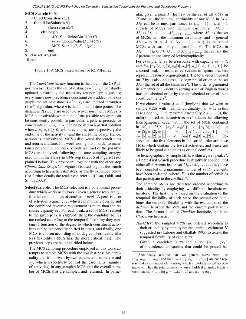
MCS-Search(P , S)1. if CheckConsistency(S)2. then if IsaSolution(S)3. then return(S)4. else begin5. MCS ← SelectVariable(P )6. pc← ChooseValue(P , MCS)7. MCS-Search(P , S ∪ {pc})8. end9. else return(Fail)10.end

Figure 1: A MCS-based solver for RCPSP/max

The CheckConsistency function is the core of the CSP al-gorithm as it keeps the set of distances d(xi, yj) constantlyupdated performing the necessary temporal propagations;every time a new precedence constraint pc is added to the Gd

graph, the set of distances d(xi, xj) are updated through aO(n2) algorithm, where n is the number of time points. Thedistances d(xi, xj) are used to discover unsolvable MCSs; aMCS is unsolvable when none of the possible resolvers canbe consistently posted. In particular, a generic precedenceconstraints pc = ai � aj can be posted in a partial solutionwhen d(ei, sj) ≥ 0, where ei and sj are respectively theend-time of the activity ai and the start-time of aj . Hence,as soon as an unsolvable MCS is discovered, the search stopsand returns a failure. It is worth noting that in order to main-tain a polynomial complexity, only a subset of the possibleMCSs are analyzed, following the same sampling strategyused within the SelectVariable step (Steps 5 of Figure 1) ex-plained below. This procedure, together with the other stepChooseValue (Steps 6 of Figure 1) is used to guide the searchaccording to heuristic estimators, as briefly explained below(for further details the reader can refer to (Cesta, Oddi, andSmith 2002)).

SelectVariable. The MCS selection is a polynomial proce-dure which works as follows. Given a generic resource rk,it relies on the notion of conflict or peak. A peak is a setof activities requiring rk, which can mutually overlap andthe combined resource requirement is more than the re-source capacity ck. For each peak, a set of MCSs relatedto the given peak is sampled; then, the candidate MCSsare ranked according to the temporal flexibility they con-tain (a function of the degree to which constituent activ-ities can be reciprocally shifted in time), and finally, oneMCS is chosen according to its degree of criticality (theless flexibility a MCS has, the more critical it is). Theprevious steps are better clarified below.

The MCS sampling procedure employed in this work at-tempts to sample MCSs with the smallest possible cardi-nality and it is driven by two parameters, namely δ andsf , which respectively control the cardinality (numberof activities) in any sampled MCS and the overall num-ber of MCSs that are sampled and returned. In partic-

ular, given a peak P , let MP be the set of all MCSs inP and mP the minimal cardinality of any MCS in MP .MP can be at most partitioned in (ck + 1) − mP + 1subsets of MCSs with identical cardinality. MP =M0 ∪ M1 ∪ . . . ∪ M(ck+1)−mP

, where M0 is the setof MCSs with the minimum cardinality, and in generalMδ , with (0 ≤ δ ≤ (ck + 1) − mP ), is the set ofMCSs with cardinality minimal plus δ. The MCSs inMP = M0 ∪ M1 ∪ . . . ∪ M(ck+1)−mP

that satisfy theδ parameter are sampled lexicographically.

For example, let rk be a resource with capacity ck = 7,and P= {a1[5], a2[3], a3[3], a4[2], a5[1], a6[1], a7[1]} bea sorted peak on resource rk (values in square bracketsrepresent resource requirements). The total order imposedon P by ≺ also induces a lexicographical order on the setMP (the set of all the MCSs in P ). This order is generatedin a manner equivalent to sorting a set of English wordsinto alphabetical order by the alphabetical order of theirconstituent letters3.

If we choose a value δ = 1 (implying that we want tosample MCSs with maximal cardinality mP + 1; in thiscase since mP = 2, maximal cardinality 2 + 1 = 3), theorder imposed on the activities in P induces the followinglexicographical order within the set of MCSs containedin M0 ∪ M1: {a1[5], a2[3]} ≺ {a1[5], a3[3]} ≺{a1[5], a4[2], a5[1]} ≺ {a1[5], a4[2], a6[1]} ≺{a1[5], a4[2], a7[1]} ≺ {a2[3], a3[3], a4[2]}. Ob-serve that the first elements in the sorted order are thoseMCSs which contain the fewest activities, and hence arelikely to be good candidates as critical conflicts.

To lexicographically sample MCSs within a given peak P ,a Depth-First Search procedure is iteratively applied untileither all elements in the set M0 ∪M1 ∪ . . . ∪Mδ havebeen sampled or a maximum number of sf |P | elementshave been collected, where |P | is the number of activitiesthat participate to the conflict P .

The sampled MCSs are therefore ordered according totheir criticality by employing two different heuristic es-timators. The first one is based on the evaluation of thetemporal flexibility of each MCS; the second one com-bines the temporal flexibility with the evaluation of thedistance between the MCS and the current partial solu-tion. The former is called TimeFlex heuristic, the latterClustering heuristic.

TimeFlex: the sampled MCSs are ordered according totheir criticality by employing the heuristic estimator Ksuggested in (Laborie and Ghallab 1995) to assess thetemporal flexibility of each MCS.

Given a candidate MCS and a set {pc1 . . . pck}of precedence constraints that could be posted be-

3Specifically, assume that two generic MCSs mcsi ={ai1, ai2, . . . , ain} and mcsl = {al1, al2, . . . , alm} are each rep-resented as a string of elements ai which are totally sorted accord-ing to ≺. Then the relation mcsi ≺ mcsl holds if an index k existssuch that aip = alp for p = 1..(k − 1) and aik ≺ alk.


45

tween pairs of activities in the MCS, K(MCS) is de-

fined as K(MCS)−1 =∑k

i=1(1 + commit(pci) −commit(pcmin))

−1 where commit(pci) ranges from0 to 1 and estimates the loss in temporal flexibilityas a result of posting constraint pci, and pcmin isthe precedence constraint with the minimum value ofcommit(pc). Note that K(MCS) (K(MCS) ∈ (0, 1])takes on its highest value of 1 in those cases whereonly one specific precedence constraint can be feasi-bly posted to resolve the conflict. In general, the closeran MCS is to being unresolvable, the higher the value ofK(MCS). It is worth noting that an MCS that is “closeto a unresolvable state” is one for which very few con-sistent activity start-time assignments remain (relativeto other MCSs), so it represents a critical case to solvefirst. When choosing which MCS to solve next, we fo-cus on the area closest to failure (i.e., the conflict selec-tion heuristic SelectVariable chooses the MCS with thehighest K value). The rationale here is that if the so-lution becomes further constrained by resolving a moretemporally flexible MCS, the probability increases thatless temporally flexible MCSs will eventually reach anunresolvable state.

Clustering: a generic decision variable MCS is eval-uated as h(MCS) = akK(MCS) + ds(MCS), alinear combination of the temporal flexibility K(MCS)and the distance ds(MCS), where ak ∈ R is aweight used to bias the contribution of the tempo-ral flexibility in the overall evaluation of the MCS.The function ds(MCS) returns an estimation of thedistance between the current partial solution Sp ={p1, pc2, . . . , pcm}4 and the MCS. In particular, ifwe consider the last δCL posted precedence constraintsSp(δCL) = {pcm−δCL+1, . . . , pcm}, 1 ≤ δ ≤ m, letAp(δCL) = {ai ∈ V : ∃pk ∈ Sp(δCL)|ai ∈ pk

5},then ds(MCS) = |Ap(δCL) ∩MCS|/|MCS|; henceds(MCS) = 1 when all the activities in MCS arein common with the already posted precedence con-straints Sp(δCL), while ds(MCS) = 0 when no ac-tivity is in common. The use of the value ds(MCS)drives the selection process of the decision variablesin a way that they tend to have activities in common,in this sense they form a cluster. Hence, precedenceconstraints tend to be posted within a cluster of criticalMCSs, with the goal of promoting early discovery of in-feasible orderings between the activities and reducingthe branching factor in the search.

ChooseValue. The opposite reasoning applies in the case ofvalue selection (which pair of activities to order and howwithin the selected MCS). In this case we attempt to retainas much temporal flexibility as possible. The conflict res-

4A solution can be represented as the set of posted precedenceconstraints pci

5each pk = ai � aj can be seen as the set of two activities{ai, aj}

olution heuristic implemented in the ChooseValue func-tion simply chooses the activity pair whose separationconstraint, when posted, preserves the highest amount oftemporal flexibility (pcmin precedence constraint), by or-dering the activities in a way similar to min-slack heuris-tics proposed in (Smith and Cheng 1993).

Horizon constraint update. The non-deterministic pro-cedure shown in Figure 1 is implemented as a depth-firstsearch, which dynamically updates the horizon constraintCi ≤ H imposed on the completion times of all the prob-lem activities, i = 1, 2, . . . , n. In particular, when the searchstart H = aHmk0, where aH is a numeric coefficient (usu-ally taking the value 3-5) and mk0 is the makespan of theproblem where the resource constraint are relaxed. Duringthe search H is dynamically updated, as soon as a new solu-tion S of the problem is discovered with makespan mk(S),then H is set to the value mk(S) − 1, as soon as this con-straints became feasible along the depth-first search pro-cess. Such additional constraint allows early pruning of al-ternatives and strongly improves the efficiency of the overallsearch procedure.

Extending MCS SearchOur extended version of CSP solver (called MCSS+) inte-grates the semantic branching idea. This is a feature thatin the SAT approach (Armando, Castellini, and Giunchiglia1999) comes for free and that in the CSP temporal rep-resentation has to be explicitly inserted. It avoids to testagain certain conditions previously proved inconsistent. Theidea behind semantic branching is the following: let us sup-pose that the MCSS+ algorithm builds a partial solutionSk = {pc1, pc2, . . . , pck} and a new decision variable isselected which has a disjunct set (precedence constraints) of

two elements {pc′ , pc′′}. Let us suppose that the disjunct

pc′

is selected first and no feasible solution exists from thepartial solution Sk ∪{pc′}. In other words, each search path

from the node Sk ∪ {pc′} arrives to an infeasible state. Inthis case, the depth-first search process removes the deci-

sion pc′

from the current solution and tries the other onepc

′′. However, even if the previous computation is not able

to find a solution, it demonstrates that with regard to the par-

tial solution Sk no solution can contain the disjunct pc′. If

we simply try pc′′

, we lose the previous information, hence,

before trying pc′′

, we add the condition ¬pc′ . That is, if

pc′= ai � aj , we add the constraint ei − sj ≥ 1 (ei and sj

are respectively the end-time of ai and the start-time of theactivity aj).

In addition, as we are performing an optimization pro-cedure, we can extend the cases where we can impose the

constraint ¬pc′ . In fact, let us suppose that from the partial

solution Sk ∪ {pc′} the best solution found has makespan

mk′. We observe that when we know a solution with

makespan mk′, we are only interested in finding a solution

with makespan mk′′< mk

′. Hence, since from Sk ∪ {pc′}


46

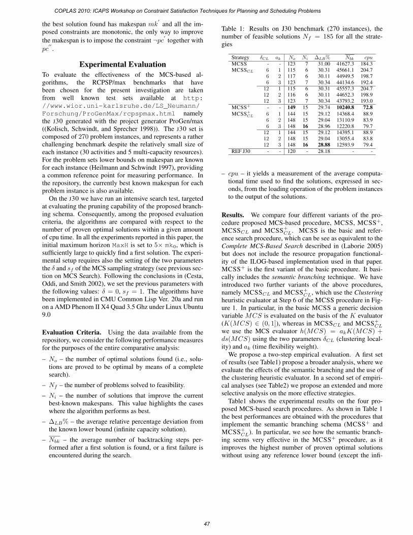
the best solution found has makespan mk′

and all the im-posed constraints are monotonic, the only way to improve

the makespan is to impose the constraint ¬pc′ together with

pc′′

.

Experimental EvaluationTo evaluate the effectiveness of the MCS-based al-gorithms, the RCPSP/max benchmarks that havebeen chosen for the present investigation are takenfrom well known test sets available at http://www.wior.uni-karlsruhe.de/LS_Neumann/Forschung/ProGenMax/rcpspmax.html namelythe J30 generated with the project generator ProGen/max((Kolisch, Schwindt, and Sprecher 1998)). The J30 set iscomposed of 270 problem instances, and represents a ratherchallenging benchmark despite the relatively small size ofeach instance (30 activities and 5 multi-capacity resources).For the problem sets lower bounds on makespan are knownfor each instance (Heilmann and Schwindt 1997), providinga common reference point for measuring performance. Inthe repository, the currently best known makespan for eachproblem instance is also available.

On the J30 we have run an intensive search test, targetedat evaluating the pruning capability of the proposed branch-ing schema. Consequently, among the proposed evaluationcriteria, the algorithms are compared with respect to thenumber of proven optimal solutions within a given amountof cpu time. In all the experiments reported in this paper, theinitial maximum horizon MaxH is set to 5× mk0, which issufficiently large to quickly find a first solution. The experi-mental setup requires also the setting of the two parametersthe δ and sf of the MCS sampling strategy (see previous sec-tion on MCS Search). Following the conclusions in (Cesta,Oddi, and Smith 2002), we set the previous parameters withthe following values: δ = 0, sf = 1. The algorithms havebeen implemented in CMU Common Lisp Ver. 20a and runon a AMD Phenom II X4 Quad 3.5 Ghz under Linux Ubuntu9.0

Evaluation Criteria. Using the data available from therepository, we consider the following performance measuresfor the purposes of the entire comparative analysis:

– No – the number of optimal solutions found (i.e., solu-tions are proved to be optimal by means of a completesearch).

– Nf – the number of problems solved to feasibility.

– Ni – the number of solutions that improve the currentbest-known makespans. This value highlights the caseswhere the algorithm performs as best.

– ΔLB% – the average relative percentage deviation fromthe known lower bound (infinite capacity solution).

– Nbk – the average number of backtracking steps per-formed after a first solution is found, or a first failure isencountered during the search.

Table 1: Results on J30 benchmark (270 instances), thenumber of feasible solutions Nf = 185 for all the strate-gies

Strategy δCL ak No Ni ΔLB% Nbk cpuMCSS - - 123 7 31.00 41627.3 184.3MCSSCL 6 1 115 6 30.31 45661.1 204.7

6 2 117 6 30.11 44949.5 198.76 3 123 7 30.34 44134.6 192.412 1 115 6 30.31 45557.3 204.712 2 116 6 30.11 44652.3 198.912 3 123 7 30.34 43793.2 193.0

MCSS+ - - 149 15 29.74 10240.8 72.8MCSS+

CL 6 1 144 15 29.12 14368.4 88.96 2 148 15 29.04 13110.9 83.96 3 148 16 28.96 12220.8 79.712 1 144 15 29.12 14395.1 88.912 2 148 15 29.04 13055.4 83.812 3 148 16 28.88 12593.9 79.4

REF J30 - - 120 - 28.18 - -

– cpu – it yields a measurement of the average computa-tional time used to find the solutions, expressed in sec-onds, from the loading operation of the problem instancesto the output of the solutions.

Results. We compare four different variants of the pro-cedure proposed MCS-based procedure, MCSS, MCSS+,MCSSCL and MCSS+

CL. MCSS is the basic and refer-ence search procedure, which can be see as equivalent to theComplete MCS-Based Search described in (Laborie 2005)but does not include the resource propagation functional-ity of the ILOG-based implementation used in that paper.MCSS+ is the first variant of the basic procedure. It basi-cally includes the semantic branching technique. We haveintroduced two further variants of the above procedures,namely MCSSCL and MCSS+

CL, which use the Clusteringheuristic evaluator at Step 6 of the MCSS procedure in Fig-ure 1. In particular, in the basic MCSS a generic decisionvariable MCS is evaluated on the basis of the K evaluator(K(MCS) ∈ (0, 1]), whereas in MCSSCL and MCSS+

CLwe use the MCS evaluator h(MCS) = akK(MCS) +ds(MCS) using the two parameters δCL (clustering local-ity) and ak (time flexibility weight).

We propose a two-step empirical evaluation. A first setof results (see Table1) propose a broader analysis, where weevaluate the effects of the semantic branching and the use ofthe clustering heuristic evaluator. In a second set of empiri-cal analyses (see Table2) we propose an extended and moreselective analysis on the more effective strategies.

Table1 shows the experimental results on the four pro-posed MCS-based search procedures. As shown in Table 1the best performances are obtained with the procedures thatimplement the semantic branching schema (MCSS+ andMCSS+

CL). In particular, we see how the semantic branch-ing seems very effective in the MCSS+ procedure, as itimproves the highest number of proven optimal solutionswithout using any reference lower bound (except the infi-


47

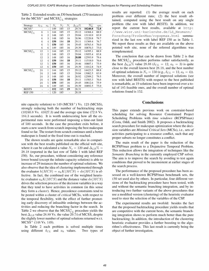
Table 2: Extended results on J30 benchmark (270 instances)for the MCSS+ and MCSS+

CL strategies

Strategy δCL ak No Nf Ni ΔLB% Nbk cpuMCSS+ - - 149 185 15 29.74 10240.8 72.8MCSS+

CL 6 1 144 185 15 29.12 14368.4 88.96 2 148 185 15 29.04 13110.9 83.96 3 148 185 16 28.96 12220.8 79.76 4 150 184 18 29.11 11369.4 76.76 5 150 185 16 29.45 10763.4 76.06 6 149 185 16 29.39 10870.3 75.0

MCSS+CL 12 1 144 185 15 29.12 14395.1 88.9

12 2 148 185 15 29.04 13055.4 83.812 3 148 185 16 28.88 12593.9 79.412 4 150 184 18 29.11 11518.0 76.612 5 150 185 16 29.46 10807.1 75.912 6 150 185 16 29.39 11012.8 74.9

MCSS+CL 24 1 144 185 15 29.12 14423.5 88.8

24 2 148 185 15 29.04 13082.5 83.924 3 148 185 16 28.92 12509.2 79.524 4 150 184 18 29.11 11503.3 76.624 5 150 185 16 29.45 10812.6 75.924 6 149 185 16 29.39 10892.5 75.0

BESTS - - 152 185 19 28.31 - -

REF J30 - - 120 185 - 28.18 - -

nite capacity solution) to 149 (MCSS+) Vs. 123 (MCSS),strongly reducing both the number of backtracking steps(10240.8 Vs. 41627.3) and the average cpu time (72.8 Vs.184.3 seconds). It is worth underscoring how all the ex-perimental runs were performed imposing a time-out limitof 500 seconds. In the case the procedure exits before, itstarts a new search from scratch imposing the best makespanfound so far. The restart from scratch continues until a bettermakespan is found or the fixed time-out is reached.

The shown results are quite remarkable also in compari-son with the best results published on the official web site,where it can be calculated a value No = 120 and ΔLB% =28.18 (reported in the last row of Table 1 with label REFJ30). So, our procedure, without considering any referencelower bound (except the infinite capacity solution) is able toincrease of 29 instances the number of optimal solutions. Wealso observe that the idea of clustering implemented throughthe evaluator h(MCS) = akK(MCS) + ds(MCS) is ef-fective. In fact, the combined use of the weighted heuris-tic evaluator akK(MCS) and the distance value ds(MCS)drives the selection process of the decision variables in a waythat they tend to have activities in common (in this sensethey form a cluster). Hence, precedence constraints tend tobe posted within a cluster of critical MCSs, with respect tothe temporal flexibility, with the effect of further promot-ing early discovery of infeasible orderings between the ac-tivities and reducing the branching factor in the search. InTable 2 we observe that the MCSS+

CL procedure yields thebest ΔLB value 28.88 Vs. the value 29.74 of MCSS, despitethe slightly lower number of optimal solutions returned w.r.t.MCSS+ (148 Vs. 149).

In Table 2 each problem is solved multiple timesusing different δCL and ak values. Two types of

results are reported: (1) the average result on eachproblem over different runs; (2) the best result ob-tained, computed using the best result on any singleproblem (the row with label BESTS). In addition, wereport the current best results, available at http://www.wior.uni-karlsruhe.de/LS_Neumann/Forschung/ProGenMax/rcpspmax.html summa-rized in the last row with label REF J30 as in Table 1.We report these results as they are available on the abovepointed web site, none of the referred algorithms wasreimplemented.

The conclusion that can be drawn from Table 2 is thatthe MCSS+

CL procedure performs rather satisfactorily, asthe best ΔLB% value 28.88 (δCL = 12, ak = 3) is quiteclose to the overall known best 28.18, and the best numberof optimal solutions is No = 150 (e.g., δCL = 12, ak = 4)).Moreover, the overall number of improved solutions (seerow with label BESTS) with respect to the best publishedis remarkable, as 19 solutions have been improved over a to-tal of 185 feasible ones, and the overall number of optimalsolutions found is 152.

Conclusions

This paper extends previous work on constraint-basedscheduling for solving Resource Constrained ProjectScheduling Problems with time windows (RCPSP/max)(Cesta, Oddi, and Smith 2002). It proposes a backtrackingsearch procedure for makespan optimization where the deci-sion variables are Minimal Critical Sets (MCSs), i.e., sets ofactivities participating to a resource conflict, such that anyproper subsets no longer constitutes a conflict.

The main result of the paper is the reduction of theRCPSP/max problem to a Disjunctive Temporal Problem.This reduction allows the integration of techniques like theSemantic Branching in the currently employed CSP solver.The aim is to improve the search by avoiding to test againconditions that proved to be inconsistent at earlier stages ofthe search process.

The performance of the proposed procedure has been as-sessed on a well-known RCPSP/max benchmark sets, theJ30 set used also by others. In particular, four different ver-sions of the backtracking procedure have been tested, withand without the semantic branching integration, and by in-troducing two further variants of the above procedures thatuse a modified version (clustering) of the heuristic evaluatorused to steer the selection of the variables of the CSP.

The experimental results are twofold: besides the factthat the proposed backtracking procedure yields results thatare competitive with the current bests, the semantic branch-ing integration shows to perform much better than the purebacktracking; In addition, the introduction of the clusteringheuristic evaluator provides a further boosting to the algo-rithm’s effectiveness. This last result is currently being theobject of further investigation.


48

AcknowledgmentsAuthors are partially supported by CNR under projectRSTL (funds 2007), EU under the ULISSE project (Con-tract FP7.218815), and MIUR under the PRIN project20089M932N (funds 2008).

ReferencesArmando, A.; Castellini, C.; and Giunchiglia,E. 1999. SAT-based Procedures for TemporalReasoning. In Proceedings 5th European Con-ference on Planning (ECP-99). (available athttp://www.mrg.dist.unige.it/˜drwho/Tsat).

Bartusch, M.; Mohring, R. H.; and Radermacher, F. J.1988. Scheduling Project Networks with Resource Con-straints and Time Windows. Annals of Operations Re-search 16:201–240.

Brucker, P.; Drexl, A.; Mohring, R.; Neumann, K.; andPesch, E. 1999. Resource-Constrained Project Scheduling:Notation, Classification, Models, and Methods. EuropeanJournal of Operations Research 112(1):3–41.

Cesta, A.; Oddi, A.; and Smith, S. 1998. Profile BasedAlgorithms to Solve Multiple Capacitated Metric Schedul-ing Problems. In AIPS-98. Proceedings of the 4th Interna-tional Conference on Artificial Intelligence Planning Sys-tems, 214–223.

Cesta, A.; Oddi, A.; and Smith, S. F. 2002. A constraint-based method for project scheduling with time windows. J.Heuristics 8(1):109–136.

Dechter, R.; Meiri, I.; and Pearl, J. 1991. Temporal con-straint networks. Artificial Intelligence 49:61–95.

Heilmann, R., and Schwindt, C. 1997. Lower Boundsfor RCPSP/max. Technical Report WIOR-511, UniversitatKarlsruhe.

Kolisch, R.; Schwindt, C.; and Sprecher, A. 1998.Benchmark Instances for Project Scheduling Problems. InWeglarz, J., ed., Handbook on Recent Advances in ProjectScheduling. Kluwer.

Laborie, P., and Ghallab, M. 1995. Planning with SharableResource Constraints. In Proceedings of the 14th Int. JointConference on Artificial Intelligence (IJCAI-95).Laborie, P. 2005. Complete mcs-based search: Applicationto resource constrained project scheduling. In IJCAI, 181–186.

Montanari, U. 1974. Networks of Constraints: Funda-mental Properties and Applications to Picture Processing.Information Sciences 7:95–132.

Neumann, K., and Schwindt, C. 1997. Activity-on-NodeNetworks with Minimal and Maximal Time Lags and TheirApplication to Make-to-Order Production. Operation Re-search Spektrum 19:205–217.

Oddi, A., and Cesta, A. 2000. Incremental Forward Check-ing for the Disjunctive Temporal Problem. In Horn, W., ed.,ECAI2000. 14th European Conference on Artificial Intelli-gence, 108–111. IOS Press.

Smith, S., and Cheng, C. 1993. Slack-Based Heuristics forConstraint Satisfaction Scheduling. In Proceedings 11thNational Conference on AI (AAAI-93).Stergiou, K., and Koubarakis, M. 1998. Backtracking Al-gorithms for Disjunctions of Temporal Constraints. In Pro-ceedings 15th National Conference on AI (AAAI-98).Stergiou, K., and Koubarakis, M. 2000. Backtracking Al-gorithms for Disjunctions of Temporal Constraints. Artifi-cial Intelligence 120(1):81–117.

Tsamardinos, I., and Pollack, M. E. 2003. Efficient so-lution techniques for disjunctive temporal reasoning prob-lems. Artif. Intell. 151(1-2):43–89.


49

Weak and Dynamic Controllability of Temporal Problemswith Disjunctions and Uncertainty

K. Brent Venable and Michele VolpatoUniversity of Padova, Italy

[email protected]@studenti.math.unipd.it

Bart PeintnerArtificial Intelligence Center

SRI International, [email protected]

Neil Yorke-SmithAmerican University of Beirut, and

SRI International, [email protected]

Abstract

The Temporal Constraint Satisfaction Problem with Uncer-tainty (TCSPU) and its disjunctive generalization, the Dis-junctive Temporal Problem with Uncertainty (DTPU), arequantitative models for temporal reasoning that account si-multaneously for disjunctive constraints and for events notunder the control of the executing agent. Such a problem isWeakly Controllable if in each possible scenario the agentcan find a decision for that scenario that satisfies all the con-straints; further, a problem is Dynamically Controllable if theagent can build a consistent decision online, as the scenariois incrementally revealed. We first consider Weak Control-lability. We present two sound and complete algorithms forchecking Weak Controllability of DTPUs. The first algorithmneeds to examine only a limited number of scenarios, but op-erates only on a restricted class of problems. The second al-gorithm is fully general, but is more expensive in terms ofspace. We then consider Dynamic Controllability. We presenta complete algorithm for testing this property for TCSPUs.Complexity results are presented for all three algorithms.

IntroductionThe Simple Temporal Problem (STP) (Dechter, Meiri, andPearl 1991) is a celebrated success of constraint-based tem-poral reasoning. Since its introduction, various effortshave extended the expressiveness of the STP, in order tomodel more realistic scheduling and planning situations.Among these extensions is the Disjunctive Temporal Prob-lem with Uncertainty (DTPU) (Venable and Yorke-Smith2005; Peintner, Venable, and Yorke-Smith 2007). TheDTPU permits non-convex and non-binary constraints, andalso accounts for time-points not under the control of the ex-ecuting agent; these are called uncontrollable time-points.

Prior work defined three concepts of controllability ofDTPUs—Strong, Weak, and Dynamic—and studied StrongControllability. A problem is Strongly Controllable if theexecuting agent can find one decision that satisfies all theconstraints under all scenarios of the uncontrollable time-points. A problem is Weakly Controllable if in each possiblescenario the agent can find a decision for that scenario thatsatisfies all of the constraints. Finally, and perhaps the most


useful notion in practice, a problem is Dynamically Control-lable if the agent can build a consistent decision online, asthe scenario is incrementally revealed.

This paper examines the two notions of controllability thathave received less attention in the literature to date. We firstconsider Weak Controllability. We present two sound andcomplete algorithms for checking Weak Controllability ofDTPUs. The first algorithm needs to examine only a lim-ited number of scenarios, but operates only on a restrictedclass of problems. The second algorithm is fully general,but is more expensive in terms of space. We then considerDynamic Controllability. We present a complete algorithmfor testing such property for the Temporal Constraint Satis-faction Problem with Uncertainty (TCSPU), a restriction ofthe DTPU that permits some amount of disjunctivity. Com-plexity results are presented for all three algorithms. Proofshave been omitted due to space limitations.

BackgroundSimple Temporal Problems with UncertaintyA Simple Temporal Problem with Uncertainty (STPU) (Vi-dal and Fargier 1998) is an STP in which uncertainty isallowed. Exogenous forces referred to as ‘Nature’ choosethe value of uncontrollable time-point variables. Naturewill ensure that the value of an uncontrollable variable (i.e.,event) respects a single contingent constraint λ−X ∈ [a, b]where X is a controllable variable, λ is the uncontrollablevariable, and a ≥ 0. An STPU is defined as a tuple< Vc, Vu, C, Cu >, where Vc and Vu are the sets of con-trollable and uncontrollable variables, respectively, C is afinite set of binary temporal constraints over Vc ∪ Vu, andCu ⊆ C is the set of contingent constraints, one for eachelement of Vu.

Given an STPU P , a decision (or control sequence) d isan assignment to the controllable variables of P , a situation(or realisation) w is a set of durations on contingent con-straints (set of elements of contingent intervals). A scheduleis a complete assignment to the variables of P , i.e., it is adecision combined with a situation. We say that a scheduleis viable if it is consistent with all the constraints. Sol(P ) isthe set of all viable schedules of P . A projection Pw corre-sponding to situation w is the STP obtained replacing eachcontingent constraint with its duration in w. Proj(P ) is the


50

set of all projections of P . A strategy S maps every projec-tion Pw into a schedule including w. A viable strategy S:Proj(P ) → Sol(P ) maps every projection Pw into a sched-ule ∈ Sol(P ) including w.

When uncontrollable variables are present the issue ofconsistency is replaced by that of controllability. Thereare three levels of controllability. In problems that exhibitStrong Controllability, there exists a time assignment to allexecutable variables that ensures all constraints will be sat-isfied whatever Nature’s realisation of the uncontrollableevents. Weak Controllability, instead, ensures the existenceof a solution for each complete situation likely to arise in theexternal world. Dynamic Controllability, finally, best suitsdynamic applications, where the effective task durations areonly observed as far as execution progresses.

An algorithm for checking Weak Controllability of ST-PUs (Vidal and Fargier 1998) uses the polynomial test forStrong Controllability, in addition to the concepts of Pseudo-controllability and Weak Controllability on bounds. AnSTPU is pseudo-controllable iff in the minimal network ofthe associated STP (i.e., considering the STPU as an STPforgetting about the distinction between contingent and exe-cutable events) no interval on a contingent constraint is tight-ened. Instead, an STPU is weakly controllable on bounds if∀w ∈ {l1, u1} × {l2, u2} × · · · × {lk, uk}, where k is thenumber of contingent constraints and li, ui are the lower andupper bounds respectively of the contingent constraint Ci,there exists a strategy S such that S(Pw) is a solution of Pw.In determining controllability, pseudo-controllability is usedas a pre-processing step, since if an STPU is weakly con-trollable then it is also pseudo-controllable. The converseis not always true. For Weak Controllability on bounds, itis proved that an STPU is weakly controllable if and onlyif it is weakly controllable on bounds (Vidal and Fargier1998). Hence, to test Weak Controllability it is sufficientto test Weak Controllability on bounds.

A dynamic execution strategy assigns a time to each con-trollable variable that may depend on the outcomes of con-tingent constraints in the past, but not on those in the fu-ture. It is shown in Morris and Muscettola (2001) that de-termining Dynamic Controllability for STPUs is tractable,and an algorithm is presented that runs in polynomial timeunder the assumption that the size of constraints werebounded. The algorithm involves repeated checking ofpseudo-controllability. In this paper we will describe an ex-tension of the Morris et al. approach to TCSPUs.

Morris and Muscettola (2005) proposed a more uniform,but less intuitive, formulation of the reductions used in theDynamic Controllability algorithm. An alternative repre-sentation is introduced for STPUs called labelled distancegraph. With this representation is possible to provide astrongly polynomial algorithm that tests Dynamic Control-lability for STPUs in O(n5) where n is the number of vari-ables. A more efficient algorithm (O(n4)) is given in Morris(2006). It reasons in terms of the absence of a particular typeof negative cycle. This is analogous to the consistency of or-dinary STP in terms of the absence of negative cycles in thedistance graph. In another work, Shah and Williams (2008)study incremental dynamic execution of STPUs.

Disjunctive Temporal Problems with UncertaintyThe Disjunctive Temporal Problem (DTP) generalizes theSTP by permitting disjunctions of time-point variables in theconstraints (Tsamardinos and Pollack 2003). A DTP withUncertainty (DTPU) (Venable and Yorke-Smith 2005) al-lows for both disjunctive constraints and contingent events.It permits constraints with two or more STPU constraints.We will sometimes call a disjunction the DTPU constraintand a disjunct the STPU constraint.

As defined in Peintner, Venable, and Yorke-Smith (2007),a DTPU is a tuple < Vc, Vu, C, Cu >, where Vc and Vu arethe sets of controllable and uncontrollable variables, respec-tively, C is a finite set of disjunctive temporal constraintsover Vc ∪ Vu, and Cu ⊆ C is the set of binary contingentconstraints, one for each element of Vu.

An exact solution of a DTPU, s = sc ∪ su is a completeassignment to all the variables V = Vc ∪ Vu that satisfies allconstraints in C. The controllable part of the solution sc isthe decision; the uncontrollable part su is the realisation.

In addition to constraints of type S (simple STP con-straints), Sc (contingent STPU constraints) and Se (ex-ecutable STPU constraints), a DTPU features the types(Peintner, Venable, and Yorke-Smith 2007):

1. DTP (D): A disjunction of two or more STP constraints(e.g., “The image action must be ended 2 minutes beforedrilling begins (controllable) or the image action must bestarted after drilling begins (controllable)”).

2. Executable DTPU (De): A disjunction of two or moreexecutable STPU disjuncts (e.g., “The image action mustend 2 minutes before drilling ends (uncontrollable) or theimage action must start at least 1 minute after drilling ends(uncontrollable)”).

3. Mixed executable DTPU (Dme): A disjunction of STPand executable STPU constraints (e.g., “The image actionmust end before drilling starts (controllable) or the imageaction must start at least 1 minute after drilling ends (un-controllable)”).

4. Contingent DTPU (Dc): A disjunction of two or morecontingent STPU constraints. Nature chooses which dis-junct will be satisfied. (e.g., “Drilling can take 5–10 min-utes or 15–20, depending on the equipment installed”).

If the set Dc of disjunctive contingent constraints of aDTPU P is empty, we call P a Simple-Natured DTPU.

Given a DTPU P , a situation w is a set of durations oncontingent constraints. A schedule is a complete assignmentto the variables of P . A schedule is viable if it is consistentwith all the constraints. Sol(P ) is the set of all viable sched-ules of P . Thus Sol(P ) is also the set of all exact solutionsof the DTP obtained by treating all contingent constraints ofP as executable constraints. A projection Pw correspond-ing to situation w is the DTP obtained replacing each con-tingent constraint with its duration in w. Proj(P ) is the setof all projections of P . A strategy S maps every projec-tion Pw into a schedule including w. A viable strategy S:Proj(P ) → Sol(P ) maps every projection Pw into a sched-ule ∈ Sol(P ) including w.


51

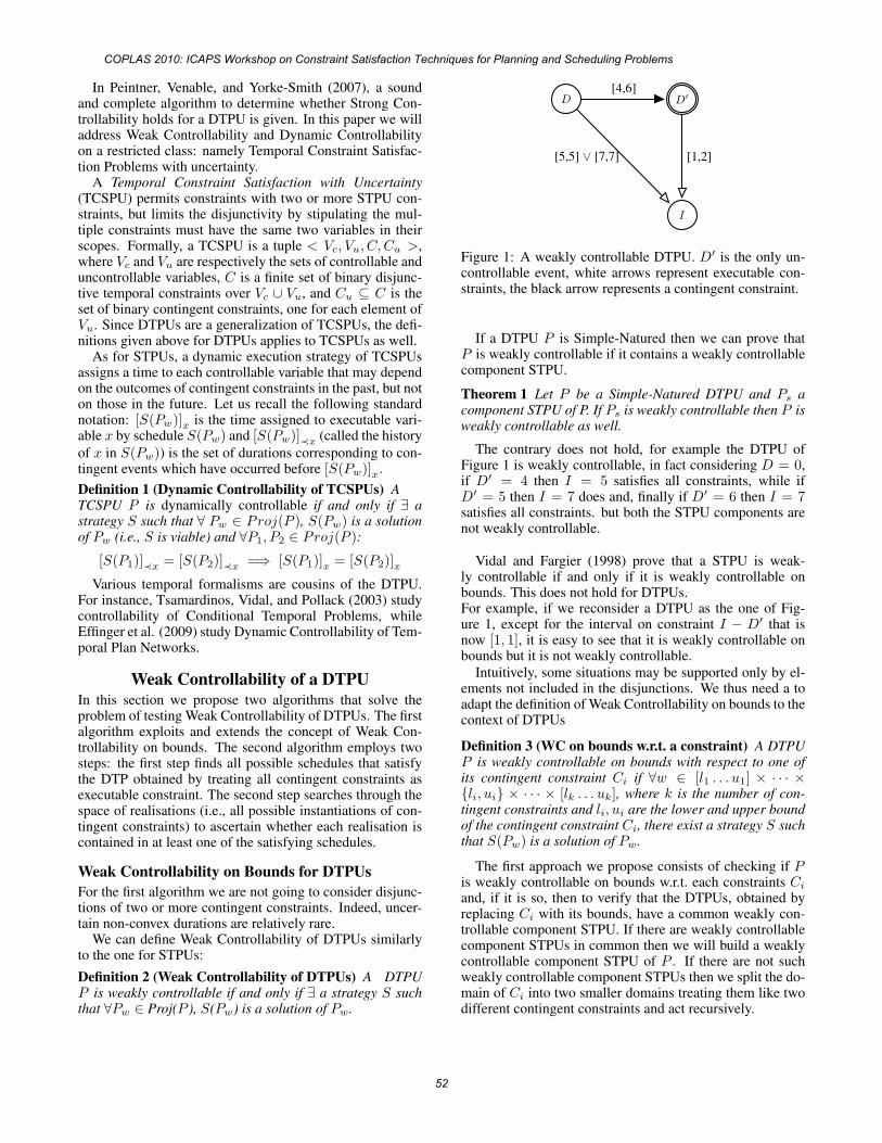
In Peintner, Venable, and Yorke-Smith (2007), a soundand complete algorithm to determine whether Strong Con-trollability holds for a DTPU is given. In this paper we willaddress Weak Controllability and Dynamic Controllabilityon a restricted class: namely Temporal Constraint Satisfac-tion Problems with uncertainty.

A Temporal Constraint Satisfaction with Uncertainty(TCSPU) permits constraints with two or more STPU con-straints, but limits the disjunctivity by stipulating the mul-tiple constraints must have the same two variables in theirscopes. Formally, a TCSPU is a tuple < Vc, Vu, C, Cu >,where Vc and Vu are respectively the sets of controllable anduncontrollable variables, C is a finite set of binary disjunc-tive temporal constraints over Vc ∪ Vu, and Cu ⊆ C is theset of binary contingent constraints, one for each element ofVu. Since DTPUs are a generalization of TCSPUs, the defi-nitions given above for DTPUs applies to TCSPUs as well.

As for STPUs, a dynamic execution strategy of TCSPUsassigns a time to each controllable variable that may dependon the outcomes of contingent constraints in the past, but noton those in the future. Let us recall the following standardnotation: [S(Pw)]x is the time assigned to executable vari-able x by schedule S(Pw) and [S(Pw)]≺x (called the history

of x in S(Pw)) is the set of durations corresponding to con-tingent events which have occurred before [S(Pw)]x.

Definition 1 (Dynamic Controllability of TCSPUs) ATCSPU P is dynamically controllable if and only if ∃ astrategy S such that ∀ Pw ∈ Proj(P ), S(Pw) is a solutionof Pw (i.e., S is viable) and ∀P1, P2 ∈ Proj(P ):

[S(P1)]≺x = [S(P2)]≺x =⇒ [S(P1)]x = [S(P2)]x

Various temporal formalisms are cousins of the DTPU.For instance, Tsamardinos, Vidal, and Pollack (2003) studycontrollability of Conditional Temporal Problems, whileEffinger et al. (2009) study Dynamic Controllability of Tem-poral Plan Networks.

Weak Controllability of a DTPUIn this section we propose two algorithms that solve theproblem of testing Weak Controllability of DTPUs. The firstalgorithm exploits and extends the concept of Weak Con-trollability on bounds. The second algorithm employs twosteps: the first step finds all possible schedules that satisfythe DTP obtained by treating all contingent constraints asexecutable constraint. The second step searches through thespace of realisations (i.e., all possible instantiations of con-tingent constraints) to ascertain whether each realisation iscontained in at least one of the satisfying schedules.

Weak Controllability on Bounds for DTPUsFor the first algorithm we are not going to consider disjunc-tions of two or more contingent constraints. Indeed, uncer-tain non-convex durations are relatively rare.

We can define Weak Controllability of DTPUs similarlyto the one for STPUs:

Definition 2 (Weak Controllability of DTPUs) A DTPUP is weakly controllable if and only if ∃ a strategy S suchthat ∀Pw ∈ Proj(P ), S(Pw) is a solution of Pw.

D D′

I

[5,5] ∨ [7,7] [1,2]

[4,6]

Figure 1: A weakly controllable DTPU. D′ is the only un-controllable event, white arrows represent executable con-straints, the black arrow represents a contingent constraint.

If a DTPU P is Simple-Natured then we can prove thatP is weakly controllable if it contains a weakly controllablecomponent STPU.

Theorem 1 Let P be a Simple-Natured DTPU and Ps acomponent STPU of P. If Ps is weakly controllable then P isweakly controllable as well.

The contrary does not hold, for example the DTPU ofFigure 1 is weakly controllable, in fact considering D = 0,if D′ = 4 then I = 5 satisfies all constraints, while ifD′ = 5 then I = 7 does and, finally if D′ = 6 then I = 7satisfies all constraints. but both the STPU components arenot weakly controllable.

Vidal and Fargier (1998) prove that a STPU is weak-ly controllable if and only if it is weakly controllable onbounds. This does not hold for DTPUs.For example, if we reconsider a DTPU as the one of Fig-ure 1, except for the interval on constraint I − D′ that isnow [1, 1], it is easy to see that it is weakly controllable onbounds but it is not weakly controllable.

Intuitively, some situations may be supported only by el-ements not included in the disjunctions. We thus need a toadapt the definition of Weak Controllability on bounds to thecontext of DTPUs

Definition 3 (WC on bounds w.r.t. a constraint) A DTPUP is weakly controllable on bounds with respect to one ofits contingent constraint Ci if ∀w ∈ [l1 . . . u1] × · · · ×{li, ui} × · · · × [lk . . . uk], where k is the number of con-tingent constraints and li, ui are the lower and upper boundof the contingent constraint Ci, there exist a strategy S suchthat S(Pw) is a solution of Pw.

The first approach we propose consists of checking if Pis weakly controllable on bounds w.r.t. each constraints Ci

and, if it is so, then to verify that the DTPUs, obtained byreplacing Ci with its bounds, have a common weakly con-trollable component STPU. If there are weakly controllablecomponent STPUs in common then we will build a weaklycontrollable component STPU of P . If there are not suchweakly controllable component STPUs then we split the do-main of Ci into two smaller domains treating them like twodifferent contingent constraints and act recursively.


52

Theorem 2 Let P be a Simple-Natured DTPU and Ci be acontingent constraint of P . Let Pli be the DTPU obtainedtightening the constraint Ci to its lower bound li and Pui

be the one obtained tightening that constraint to its upperbound ui. If both Pli and Pui

are weakly controllable and ifthey have a common weakly controllable component STPUthen P is weakly controllable as well.

Exploiting Weak Controllability on bounds:DTPU-WC-BoundsThe result in the previous section suggests a way to testthe Weak Controllability of a DTPU. We can check WeakControllability of Pli and Pui

recursively by tightening re-spectively to its lower and upper bound one by one each re-maining contingent constraint. When there are no more con-straints to tighten we have DTPs and we can check consis-tency for those. By verifying the intersection of their sets ofsolutions, without considering the last contingent constraintthat cannot be the same in the solutions of Pli and Pui

, wecan decide Weak Controllability for the last DTPU.

If the intersection is empty, then we must split the domainof Ci into two smaller domains obtaining two different DT-PUs. if both of them are weakly controllable then we cansay that the initial DTPU is weakly controllable.

In what follows we will use the following notation: wewill denote with SC the set of contingent single disjunctconstraints, with CD the set of multi-disjunct constraints(D ∪ De ∪ Dme), and with CS all others (S ∪ Se). DTPU-WC-Bounds receives as input the three sets of constraints andreturns the set of component STPUs that are weakly control-lable and whether the DTPU is weakly controllable or not;if there is no weakly controllable component STPU then itreturns an empty set. The algorithm is composed by two mu-tually recursive functions, DTPU-WC and CheckIntersection.

DTPU-WC checks if there are contingent constraints to beprocessed. If there are none then it returns all the solutionsof the current associated DTP. Otherwise it checks WeakControllability on bounds for current DTPU by choosing acontingent constraint and replacing it with its lower (resp.upper) bound obtaining two different DTPUs, L and U . Ifboth of them are weakly controllable then the initial DTPUis weakly controllable on bounds and the algorithm mustverify with CheckIntersection if they have a common com-ponent STPUs.

Pseudocode is given in Algorithm 1. Line 1 is the exitcondition for the recursion that is triggered when a full re-alisation is built, in this case all the contingent constraintshave been instantiated. The DTPU becomes a classical DTPand Weak Controllability is equivalent to classical consis-tency. If the DTP is consistent then it is weakly controllableand (line 4) we return the set of solutions in form of STPs,otherwise (line 3) we return an empty set followed by thefact that it is not weakly controllable.

If there are contingent constraints then a contingent con-straint Ci is removed from SC and replaced with its lowerbound, DTPU-WC checks Weak Controllability and does thesame for the upper bound. If the presence of a non-weaklycontrollable DTPU is detected then the execution is stoppedand DTPU-WC returns (� , false) (lines 9 and 12).

Algorithm 1 DTPU-WC-Bounds

DTPU-WC(SC , CD, CS)

1: if SC = � then2: sol ← DTP-Solutions(CD, CS ) {it’s a DTP: solve and return its solutions}3: if sol = � then return (� , false) {not WC}4: else return (sol , true) {this DTP is consistent, return the set of solutions }5: else6: choose and remove Ci from SC {Ci is a simple contingent constraint}7: C′

S ← CS ∪ {Xi1 −Xi2 ∈ [li, li]} {Ci is in the form

{Xi1 − Xi2 ∈ [li, ui]} }8: L ← DTPU-WC(SC , CD, C′

S)9: if L = (� , false) then return (� , false) {found inconsistent DTP}

10: C′′S ← CS ∪ {Xi1 −Xi2 ∈ [ui, ui]}

11: U ← DTPU-WC(SC , CD, C′′S )

12: if U = (� , false) then return (� , false) {found inconsistent

DTP}13: return CheckIntersection(SC , CD, CS , li, ui, L, U )

CheckIntersection(SC , CD, CS , li, ui, L, U )

1: if L ∩ U �= � then return ((L ∩ U)[Ci ← [li, ui]] , true)2: if ui − li = 1 then return (� , true) {li and ui are consecutive, there is

nothing to split}3: choose a ki such that li < ki < ui {there is no WC STPU component,}4: C′

S ← CS ∪ {Xi1 −Xi2 ∈ [ki, ki]} {so we need to split the contingent

constraint in two parts}5: K ← DTPU-WC(SC , CD, C′

S)6: if K = (� , false) then return (� , false) {a part is not weakly

controllable}7: inf ← CheckIntersection(SC , CD, CS , li, ki, L,K)8: sup ← CheckIntersection(SC , CD, CS , ki, ui,K, U )9: if inf �= (� , false) AND sup �= (� , false) then

10: return (� , true) {the two parts are WC and so the whole is WC}else return(� , false)

Once DTPU-WC has checked Weak Controllability onbounds it has to call CheckIntersection to be sure that WeakControllability is ensured (line 13).

Procedure CheckIntersection verifies that the intersectionsof weakly controllable component STPUs of the DTPUs ob-tained tightening the constraint Ci to its lower and upperbounds are not empty (line 1). In this case we have at leasta component STPU for the initial DTPU that is weakly con-trollable and so we return the set of all weakly controllablecomponents adding Ci to each of them.

Otherwise, if the intersection is empty, we have to split theinterval of Ci into two different intervals (line 3) and checkthe two obtained DTPUs recursively (lines 7 and 8).

If Ci cannot be further split and the two DTPUs corre-sponding to the li branch and ui branch are weakly con-trollable then if we join li and ui into a single contingentconstraint we obtain a weakly controllable DTPU. However,in addition to returning ‘true’, we also return an empty setof supporting STPUs (since there is not a common weaklycontrollable component STPU, line 2).

Example 1 Consider the DTPU of Figure 2, which has twouncontrollable variables: D′ and A′. For the sake of com-pactness we call C1 constraint A′ − A ∈ [4, 6] and C2

constraint D′ − D ∈ [0, 5]. Moreover we call d1 disjunctD − A ∈ [5, 5], d2 disjunct D − A ∈ [7, 7], d3 disjunct


53

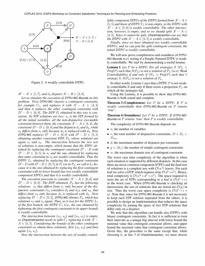
A A′

B B′

D

D′

[5,5] ∨ [7,7]

[2,5]

[1,2]

[0,6]

[3,5]

[4,6]

[0,5]

B′ −A′ ∈ [1, 7] ∨A′ −B ∈ [2, 8]

Figure 2: A weakly controllable DTPU.

B′ −A′ ∈ [1, 7], and d4 disjunct A′ −B ∈ [2, 8].Let us simulate the execution of DTPU-WC-Bounds on this

problem. First DTPU-WC chooses a contingent constraint,for example C1, and replaces it with A′ − A ∈ [4, 4]and then it replaces the other contingent constraint withD′ − D ∈ [0, 0]. The DTP P1 obtained in this way is con-sistent. Its STP solutions are two: s1 is the STP formed byall the initial variables, all the non-disjunctive executableconstraint between them, the constraint A′ −A ∈ [4, 4], theconstraint D′−D ∈ [0, 0] and the disjuncts d1 and d3, whiles2 differs from s1 only because d3 is replaced with d4. NowDTPU-WC replaces D′ − D ∈ [0, 0] with D′ − D ∈ [5, 5]obtaining another consistent DTP, P2, whose solutions areagain s1 and s2. The intersection between the two setsof solutions is non-empty, which means that the STPU ob-tained by replacing the contingent constraint D′ − D withD′ − D ∈ [0, 5] in s1 and the one obtained by replacingthat same constraint in s2 are weakly controllable. Thus theDTPU L1 obtained by replacing the contingent constraintD′−D with D′−D ∈ [0, 5] in P1 (or in P2; we call it L1 be-cause it is the one obtained by replacing the first contingentconstraint with its lower bound) has two weakly controllablecomponent STPUs and thus it is weakly controllable.

The execution proceeds to consider A′ − A ∈ [6, 6] andD′ − D ∈ [0, 0]. The DTP obtained, P3, has the followingsolutions: s3 that differs from s1 only because of the dis-junctive constraints (s3 considers d2 and d3), and s4, thatdiffers from s3 only because d3 is replaced with d4. Nextreplacing D′ −D ∈ [5, 5], DTPU-WC obtains P4, which hassolutions s3 and s4 again. Thus, as it was for the DTPU L1

of the first branch, the DTPU U1 (i.e., the one obtained bytightening the first contingent constraint to its upper bound)is weakly controllable.

The intersection between {s1, s2} and {s3, s4} is empty,so CheckIntersection needs to split C1 replacing it with A′ −A ∈ [5, 5]. Considering the bounds of the other contingentconstraint we obtain these solutions: first {s3, s4} and thenagain {s3, s4}.

Now the intersection between the sets of weakly control-

lable component STPUs of the DTPU formed from A′−A ∈[5, 5] and those of DTPU U1 is non-empty, so the DTPU withA′ − A ∈ [5, 6] is weakly controllable. The other intersec-tion, however, is empty, and so we should split A′ − A ∈[4, 5]. Since it cannot be split, CheckIntersection can say thatthe DTPU with A′ −A ∈ [4, 5] is weakly controllable.

Finally, since we have obtained two weakly controllableDTPUs, and we can join the split contingent constraint, theinitial DTPU is weakly controllable.

We will now prove completeness and soundness of DTPU-WC-Bounds w.r.t. testing if a Simple-Natured DTPU is weak-ly controllable. We start by demonstrating a useful lemma.

Lemma 1 Let P be a DTPU. For all strategies S ∃Pw ∈Proj(P ) such that S(Pw) is not a solution of Pw (w.r.t. WeakControllability) if and only if ∃Pw ∈ Proj(P ) such that ∀strategy S, S(Pw) is not a solution of Pw.

In other words, Lemma 1 says that a DTPU P is not weak-ly controllable if and only if there exists a projection Pw onwhich all the strategies fail.

Using the Lemma, it is possible to show that DTPU-WC-Bounds is both sound and complete.

Theorem 3 (Completeness) Let P be a DTPU. If P isweakly controllable then DTPU-WC-Bounds on P returns‘true’.

Theorem 4 (Soundness) Let P be a DTPU. If DTPU-WC-Bounds on P returns ‘true’ then P is weakly controllable.

The complexity of DTPU-WC-Bounds depends on:

• n, the number of variables

• e, the total number of disjunctive constraints, D +De +Dme.

• d, the maximum number of disjuncts per constraint

• q = |SC |, the number of simple contingent constraints

• w, the maximum domain size of contingent constraint

The worst case time complexity of the algorithm is wheneach situation is supported by different disjuncts. In this casethere are never common component STPUs and the final treeof solutions is a complete tree with O(wq) leaves. For eachleaf we solve a DTP, which requires time O(de∗n2). Hence,total complexity is O(wq ∗ de ∗ n2). The space required tostore the set of STPs corresponding to a leaf is O(de ∗ e)in the worst case. When DTPU-WC-Bounds is checking anintersection, the sets of solutions that are stored are O(q) insize. Thus the worst case space complexity is O(de ∗ e ∗q). Note that, since for DTPU-WC-Bounds it is not necessaryto keep each STP solution separated from the others, it ispossible to design an implementation that reduces the spacecomplexity by joining the space of two STP solutions thatdiffer only on a disjunct.

We note that this algorithm can handle also DTPUs withbinary contingent constraints. In fact it is sufficient to treattheir intervals as a unique big interval with lower bound theminimal value that contingent constraint allows, and upperbound the maximal value that contingent constraint allows.Given this, the procedure is the same except that, whilechoosing k, at line 3 of CheckIntersection, we must choose


54

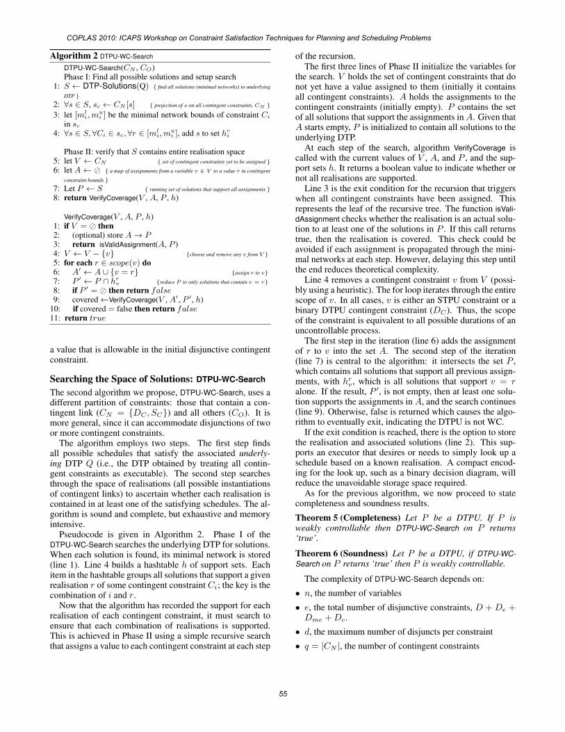
Algorithm 2 DTPU-WC-Search

DTPU-WC-Search(CN , CO)Phase I: Find all possible solutions and setup search

1: S ← DTP-Solutions(Q) { find all solutions (minimal networks) to underlying

DTP }2: ∀s ∈ S, sc ← CN [s] { projection of s on all contingent constraints, CN }3: let [ml

i,mui ] be the minimal network bounds of constraint Ci

in sc4: ∀s ∈ S, ∀Ci ∈ sc, ∀r ∈ [ml

i,mui ], add s to set hr

i

Phase II: verify that S contains entire realisation space5: let V ← CN { set of contingent constraints yet to be assigned }6: let A ← � { a map of assignments from a variable v ∈ V to a value r in contingent

constraint bounds }7: Let P ← S { running set of solutions that support all assignments }8: return VerifyCoverage(V , A, P , h)

VerifyCoverage(V , A, P , h)1: if V = � then2: (optional) store A → P3: return isValidAssignment(A, P )4: V ← V − {v} {choose and remove any v from V }5: for each r ∈ scope(v) do6: A′ ← A ∪ {v = r} {assign r to v}7: P ′ ← P ∩ hr

v {reduce P to only solutions that contain v = r}8: if P ′ = � then return false9: covered ←VerifyCoverage(V , A′, P ′, h)

10: if covered = false then return false11: return true

a value that is allowable in the initial disjunctive contingentconstraint.

Searching the Space of Solutions: DTPU-WC-Search

The second algorithm we propose, DTPU-WC-Search, uses adifferent partition of constraints: those that contain a con-tingent link (CN = {DC , SC}) and all others (CO). It ismore general, since it can accommodate disjunctions of twoor more contingent constraints.

The algorithm employs two steps. The first step findsall possible schedules that satisfy the associated underly-ing DTP Q (i.e., the DTP obtained by treating all contin-gent constraints as executable). The second step searchesthrough the space of realisations (all possible instantiationsof contingent links) to ascertain whether each realisation iscontained in at least one of the satisfying schedules. The al-gorithm is sound and complete, but exhaustive and memoryintensive.

Pseudocode is given in Algorithm 2. Phase I of theDTPU-WC-Search searches the underlying DTP for solutions.When each solution is found, its minimal network is stored(line 1). Line 4 builds a hashtable h of support sets. Eachitem in the hashtable groups all solutions that support a givenrealisation r of some contingent constraint Ci; the key is thecombination of i and r.

Now that the algorithm has recorded the support for eachrealisation of each contingent constraint, it must search toensure that each combination of realisations is supported.This is achieved in Phase II using a simple recursive searchthat assigns a value to each contingent constraint at each step

of the recursion.The first three lines of Phase II initialize the variables for

the search. V holds the set of contingent constraints that donot yet have a value assigned to them (initially it containsall contingent constraints). A holds the assignments to thecontingent constraints (initially empty). P contains the setof all solutions that support the assignments in A. Given thatA starts empty, P is initialized to contain all solutions to theunderlying DTP.

At each step of the search, algorithm VerifyCoverage iscalled with the current values of V , A, and P , and the sup-port sets h. It returns a boolean value to indicate whether ornot all realisations are supported.

Line 3 is the exit condition for the recursion that triggerswhen all contingent constraints have been assigned. Thisrepresents the leaf of the recursive tree. The function isVali-dAssignment checks whether the realisation is an actual solu-tion to at least one of the solutions in P . If this call returnstrue, then the realisation is covered. This check could beavoided if each assignment is propagated through the mini-mal networks at each step. However, delaying this step untilthe end reduces theoretical complexity.

Line 4 removes a contingent constraint v from V (possi-bly using a heuristic). The for loop iterates through the entirescope of v. In all cases, v is either an STPU constraint or abinary DTPU contingent constraint (DC). Thus, the scopeof the constraint is equivalent to all possible durations of anuncontrollable process.

The first step in the iteration (line 6) adds the assignmentof r to v into the set A. The second step of the iteration(line 7) is central to the algorithm: it intersects the set P ,which contains all solutions that support all previous assign-ments, with hr

v , which is all solutions that support v = ralone. If the result, P ′, is not empty, then at least one solu-tion supports the assignments in A, and the search continues(line 9). Otherwise, false is returned which causes the algo-rithm to eventually exit, indicating the DTPU is not WC.

If the exit condition is reached, there is the option to storethe realisation and associated solutions (line 2). This sup-ports an executor that desires or needs to simply look up aschedule based on a known realisation. A compact encod-ing for the look up, such as a binary decision diagram, willreduce the unavoidable storage space required.

As for the previous algorithm, we now proceed to statecompleteness and soundness results.

Theorem 5 (Completeness) Let P be a DTPU. If P isweakly controllable then DTPU-WC-Search on P returns‘true’.

Theorem 6 (Soundness) Let P be a DTPU, if DTPU-WC-Search on P returns ‘true’ then P is weakly controllable.

The complexity of DTPU-WC-Search depends on:

• n, the number of variables

• e, the total number of disjunctive constraints, D +De +Dme +Dc.

• d, the maximum number of disjuncts per constraint

• q = |CN |, the number of contingent constraints


55

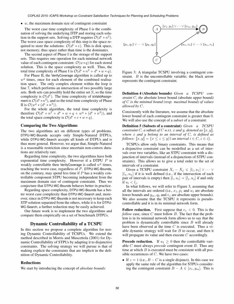
• w, the maximum domain size of contingent constraint

The worst case time complexity of Phase I is the combi-nation of solving the underlying DTP and storing each solu-tion in the support sets. Solving a DTP requires O(de ∗ n2).The worst case space complexity of this step is the space re-quired to store the solutions: O(de ∗ e). This is disk space,not memory; thus space rather than time is the dominates.

The second aspect of Phase I is the storage of the supportsets. This requires one operation for each minimal networkvalue of each contingent constraint: O(w∗q) for each storedsolution. This is the space complexity as well. Thus, thetotal time complexity of Phase I is O(de ∗ n2 + de ∗w ∗ q).

For Phase II, the VerifyCoverage algorithm is called up towq times, once for each element of the combined realisa-tion space. The only complex element within the loop isline 7, which performs an intersection of two possibly largesets. Both sets can possibly hold the entire set S, so the timecomplexity is O(de). The time complexity of isValidAssign-ment is O(de∗n3), and so the total time complexity of PhaseII is O(wq ∗ (de ∗ n3)).

For the whole algorithm, the total time complexity istherefore O(de ∗ n2 + de ∗ w ∗ q + wq ∗ (de ∗ n3)), andthe total space complexity is O(de ∗ e ∗ w ∗ q).Comparing the Two AlgorithmsThe two algorithms act on different types of problems.DTPU-WC-Bounds accepts only Simple-Natured DTPUs,while DTPU-WC-Search accepts all kinds of DTPUs and isthus more general. However, we argue that, Simple-Naturedis a reasonable restriction since uncertain non-convex dura-tions are relatively rare.

Regarding time complexity, the two algorithms have bothexponential time complexity. However if a DTPU P isweakly controllable then VerifyCoverage is called wq times,reaching the worst case, regardless of P . DTPU-WC-Bounds,on the contrary, may spend less time if P has a weakly con-trollable component STPU becoming independent from themaximum domain size of contingent constraint. Thus weconjecture that DTPU-WC-Bounds behaves better in practice.

Regarding space complexity, DTPU-WC-Bounds has a bet-ter worst case complexity than DTPU-WC-Search and, more-over, since in DTPU-WC-Bounds is not necessary to keep eachSTP solution separated from the others, while it is for DTPU-WC-Search, a further reduction may be easily achieved.

Our future work is to implement the two algorithms andcompare them empirically on a set of benchmark DTPUs.

Dynamic Controllability of a TCSPUIn this section we propose a complete algorithm for test-ing Dynamic Controllability of TCSPUs. We extend themethod described in Morris and Muscettola (2001) for Dy-namic Controllability of STPUs by adapting it to disjunctiveconstraints. The solving strategy we will pursue is that ofmaking explicit the constraints that are implicit in the defi-nition of Dynamic Controllability.

ReductionsWe start by introducing the concept of absolute bounds:

A B

C

[p1, q1] ∨ · · · ∨ [pk, qk] [u1, v1] ∨ · · · ∨ [uz, vz]

[x1, y1] ∨ · · · ∨ [xm, ym]

Figure 3: A triangular TCSPU involving a contingent con-straint. B is the uncontrollable variable; the black arrowrepresents the contingent constraint.

Definition 4 (Absolute bounds) Given a TCSPU con-straint C, the absolute lower bound (absolute upper bound)of C is the minimal bound (resp. maximal bound) of valuesallowed by C.

Consistently with the literature, we assume that the absolutelower bound of each contingent constraint is greater than 0.We will also use the concept of a subset of a constraint:

Definition 5 (Subsets of a constraint) Given a TCSPUconstraint C, a subset of C w.r.t. x and y, denoted as �x, y�,where x and y belong to an interval of C, is defined asfollows: �x, y� = {x ≤ z ≤ y|∃ an interval i ∈ C, z ∈ i}.

TCSPUs allow only binary constraints. This means thata disjunctive constraint can be modelled as a set of inter-vals over two variables, like an STPU constraint with a dis-junction of intervals (instead of a disjunctions of STPU con-straints). This allows us to give a total order to the set ofintervals of a constraint.

Given a TCSPU constraint Xi − Xj ∈ [l1, u1] ∨ · · · ∨[ln, un] if it is well defined (i.e., if the intersection of eachpair of intervals is empty) then [li, ui] ≺ [lj , uj ] if and onlyif ui < lj .

In what follows, we will refer to Figure 3, assuming thatall the intervals are ordered (i.e., x1, p1 and u1 are absolutelower bounds and ym, qk and vz are absolute upper bounds).We also assume that the TCSPU it represents is pseudo-controllable and it is in its minimal network form.

Follow reduction. First suppose that vz < 0. This is thefollow case, since C must follow B. The fact that the prob-lem is in its minimal network form allows us to say that theproblem is dynamically controllable since B will alreadyhave been observed at the time C is executed. Thus a vi-able dynamic strategy will wait for B to occur, and then itwill propagate its value and then execute C accordingly.

Precede reduction. If u1 ≥ 0 then the controllable vari-able C must always precede contingent event B. Thus anytime at which B is executed must be consistent with all pos-sible occurrences of C. We have two cases:

• If z = 1 (i.e., B − C is a single disjunct). In this case weapply the same rule of the algorithm for STPUs consider-ing the contingent constraint B − A ∈ [x1, ym]. This is


56

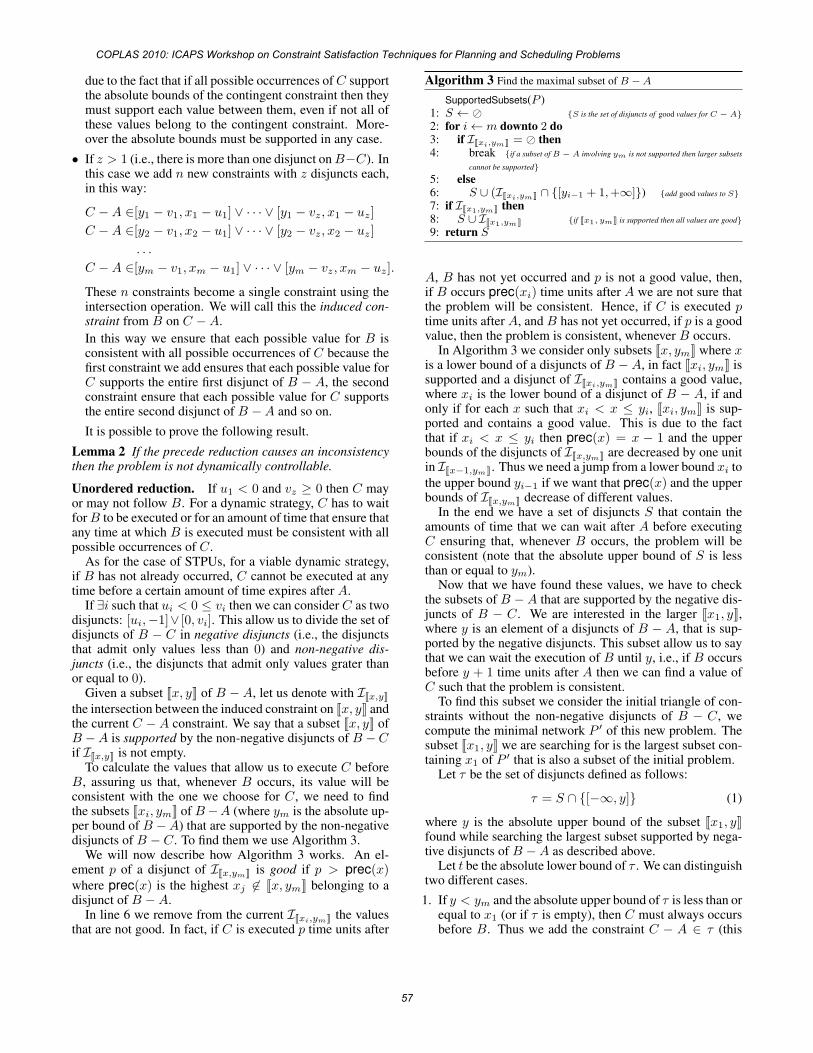
due to the fact that if all possible occurrences of C supportthe absolute bounds of the contingent constraint then theymust support each value between them, even if not all ofthese values belong to the contingent constraint. More-over the absolute bounds must be supported in any case.

• If z > 1 (i.e., there is more than one disjunct on B−C). Inthis case we add n new constraints with z disjuncts each,in this way:

C −A ∈[y1 − v1, x1 − u1] ∨ · · · ∨ [y1 − vz, x1 − uz]

C −A ∈[y2 − v1, x2 − u1] ∨ · · · ∨ [y2 − vz, x2 − uz]

. . .

C −A ∈[ym − v1, xm − u1] ∨ · · · ∨ [ym − vz, xm − uz].

These n constraints become a single constraint using theintersection operation. We will call this the induced con-straint from B on C −A.

In this way we ensure that each possible value for B isconsistent with all possible occurrences of C because thefirst constraint we add ensures that each possible value forC supports the entire first disjunct of B − A, the secondconstraint ensure that each possible value for C supportsthe entire second disjunct of B −A and so on.

It is possible to prove the following result.

Lemma 2 If the precede reduction causes an inconsistencythen the problem is not dynamically controllable.

Unordered reduction. If u1 < 0 and vz ≥ 0 then C mayor may not follow B. For a dynamic strategy, C has to waitfor B to be executed or for an amount of time that ensure thatany time at which B is executed must be consistent with allpossible occurrences of C.

As for the case of STPUs, for a viable dynamic strategy,if B has not already occurred, C cannot be executed at anytime before a certain amount of time expires after A.

If ∃i such that ui < 0 ≤ vi then we can consider C as twodisjuncts: [ui,−1]∨ [0, vi]. This allow us to divide the set ofdisjuncts of B − C in negative disjuncts (i.e., the disjunctsthat admit only values less than 0) and non-negative dis-juncts (i.e., the disjuncts that admit only values grater thanor equal to 0).

Given a subset �x, y� of B − A, let us denote with I�x,y�

the intersection between the induced constraint on �x, y� andthe current C − A constraint. We say that a subset �x, y� ofB −A is supported by the non-negative disjuncts of B −Cif I�x,y� is not empty.

To calculate the values that allow us to execute C beforeB, assuring us that, whenever B occurs, its value will beconsistent with the one we choose for C, we need to findthe subsets �xi, ym� of B−A (where ym is the absolute up-per bound of B −A) that are supported by the non-negativedisjuncts of B − C. To find them we use Algorithm 3.

We will now describe how Algorithm 3 works. An el-ement p of a disjunct of I�x,ym� is good if p > prec(x)where prec(x) is the highest xj �∈ �x, ym� belonging to adisjunct of B −A.

In line 6 we remove from the current I�xi,ym� the valuesthat are not good. In fact, if C is executed p time units after

Algorithm 3 Find the maximal subset of B −A

SupportedSubsets(P )1: S ← � {S is the set of disjuncts of good values for C − A}2: for i ← m downto 2 do3: if I�xi,ym� = � then4: break {if a subset of B − A involving ym is not supported then larger subsets

cannot be supported}5: else6: S ∪ (I�xi,ym� ∩ {[yi−1 + 1,+∞]}) {add good values to S}7: if I�x1,ym� then8: S ∪ I�x1,ym� {if �x1, ym� is supported then all values are good}9: return S

A, B has not yet occurred and p is not a good value, then,if B occurs prec(xi) time units after A we are not sure thatthe problem will be consistent. Hence, if C is executed ptime units after A, and B has not yet occurred, if p is a goodvalue, then the problem is consistent, whenever B occurs.

In Algorithm 3 we consider only subsets �x, ym� where xis a lower bound of a disjuncts of B − A, in fact �xi, ym� issupported and a disjunct of I�xi,ym� contains a good value,where xi is the lower bound of a disjunct of B − A, if andonly if for each x such that xi < x ≤ yi, �xi, ym� is sup-ported and contains a good value. This is due to the factthat if xi < x ≤ yi then prec(x) = x − 1 and the upperbounds of the disjuncts of I�x,ym� are decreased by one unitin I�x−1,ym�. Thus we need a jump from a lower bound xi to

the upper bound yi−1 if we want that prec(x) and the upperbounds of I�x,ym� decrease of different values.

In the end we have a set of disjuncts S that contain theamounts of time that we can wait after A before executingC ensuring that, whenever B occurs, the problem will beconsistent (note that the absolute upper bound of S is lessthan or equal to ym).

Now that we have found these values, we have to checkthe subsets of B −A that are supported by the negative dis-juncts of B − C. We are interested in the larger �x1, y�,where y is an element of a disjuncts of B − A, that is sup-ported by the negative disjuncts. This subset allow us to saythat we can wait the execution of B until y, i.e., if B occursbefore y + 1 time units after A then we can find a value ofC such that the problem is consistent.

To find this subset we consider the initial triangle of con-straints without the non-negative disjuncts of B − C, wecompute the minimal network P ′ of this new problem. Thesubset �x1, y� we are searching for is the largest subset con-taining x1 of P ′ that is also a subset of the initial problem.

Let τ be the set of disjuncts defined as follows:

τ = S ∩ {[−∞, y]} (1)

where y is the absolute upper bound of the subset �x1, y�found while searching the largest subset supported by nega-tive disjuncts of B −A as described above.

Let t be the absolute lower bound of τ . We can distinguishtwo different cases.

1. If y < ym and the absolute upper bound of τ is less than orequal to x1 (or if τ is empty), then C must always occursbefore B. Thus we add the constraint C − A ∈ τ (this


57

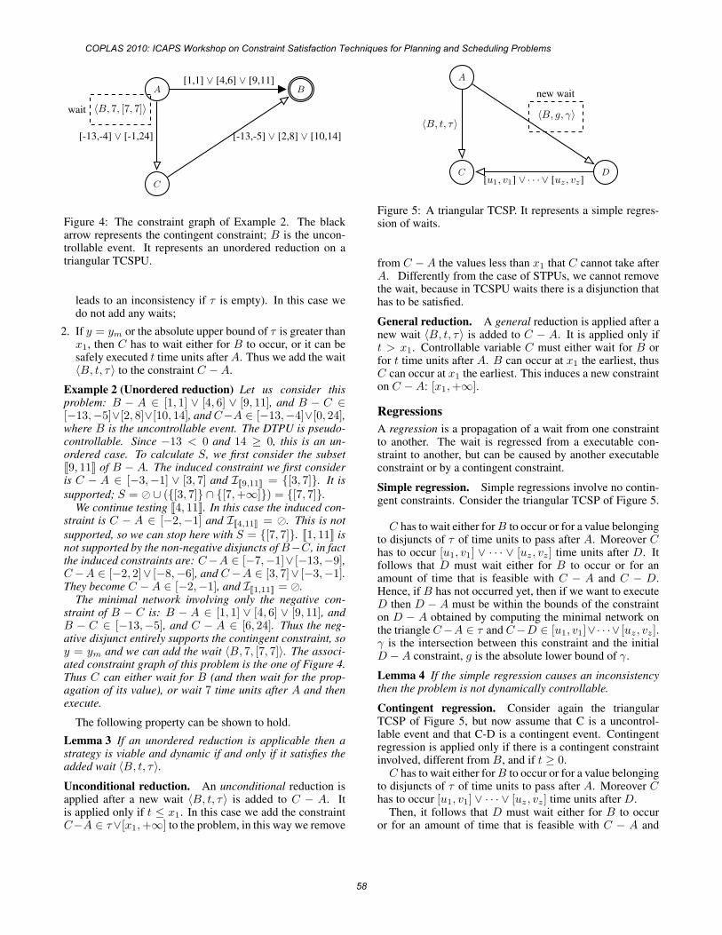
A B

C

[-13,-4] ∨ [-1,24] [-13,-5] ∨ [2,8] ∨ [10,14]

[1,1] ∨ [4,6] ∨ [9,11]

〈B, 7, [7, 7]〉wait

Figure 4: The constraint graph of Example 2. The blackarrow represents the contingent constraint; B is the uncon-trollable event. It represents an unordered reduction on atriangular TCSPU.

leads to an inconsistency if τ is empty). In this case wedo not add any waits;

2. If y = ym or the absolute upper bound of τ is greater thanx1, then C has to wait either for B to occur, or it can besafely executed t time units after A. Thus we add the wait〈B, t, τ〉 to the constraint C −A.

Example 2 (Unordered reduction) Let us consider thisproblem: B − A ∈ [1, 1] ∨ [4, 6] ∨ [9, 11], and B − C ∈[−13,−5]∨[2, 8]∨[10, 14], and C−A ∈ [−13,−4]∨[0, 24],where B is the uncontrollable event. The DTPU is pseudo-controllable. Since −13 < 0 and 14 ≥ 0, this is an un-ordered case. To calculate S, we first consider the subset�9, 11� of B − A. The induced constraint we first consideris C − A ∈ [−3,−1] ∨ [3, 7] and I�9,11� = {[3, 7]}. It issupported; S = � ∪ ({[3, 7]} ∩ {[7,+∞]}) = {[7, 7]}.

We continue testing �4, 11�. In this case the induced con-straint is C − A ∈ [−2,−1] and I�4,11� = �. This is notsupported, so we can stop here with S = {[7, 7]}. �1, 11� isnot supported by the non-negative disjuncts of B−C, in factthe induced constraints are: C−A ∈ [−7,−1]∨ [−13,−9],C−A ∈ [−2, 2]∨ [−8,−6], and C−A ∈ [3, 7]∨ [−3,−1].They become C −A ∈ [−2,−1], and I�1,11� = �.

The minimal network involving only the negative con-straint of B − C is: B − A ∈ [1, 1] ∨ [4, 6] ∨ [9, 11], andB − C ∈ [−13,−5], and C − A ∈ [6, 24]. Thus the neg-ative disjunct entirely supports the contingent constraint, soy = ym and we can add the wait 〈B, 7, [7, 7]〉. The associ-ated constraint graph of this problem is the one of Figure 4.Thus C can either wait for B (and then wait for the prop-agation of its value), or wait 7 time units after A and thenexecute.

The following property can be shown to hold.

Lemma 3 If an unordered reduction is applicable then astrategy is viable and dynamic if and only if it satisfies theadded wait 〈B, t, τ〉.Unconditional reduction. An unconditional reduction isapplied after a new wait 〈B, t, τ〉 is added to C − A. Itis applied only if t ≤ x1. In this case we add the constraintC−A ∈ τ∨[x1,+∞] to the problem, in this way we remove

A

C D

〈B, t, τ〉

[u1, v1] ∨ · · · ∨ [uz, vz]

〈B, g, γ〉new wait

Figure 5: A triangular TCSP. It represents a simple regres-sion of waits.

from C − A the values less than x1 that C cannot take afterA. Differently from the case of STPUs, we cannot removethe wait, because in TCSPU waits there is a disjunction thathas to be satisfied.

General reduction. A general reduction is applied after anew wait 〈B, t, τ〉 is added to C − A. It is applied only ift > x1. Controllable variable C must either wait for B orfor t time units after A. B can occur at x1 the earliest, thusC can occur at x1 the earliest. This induces a new constrainton C −A: [x1,+∞].

RegressionsA regression is a propagation of a wait from one constraintto another. The wait is regressed from a executable con-straint to another, but can be caused by another executableconstraint or by a contingent constraint.

Simple regression. Simple regressions involve no contin-gent constraints. Consider the triangular TCSP of Figure 5.

C has to wait either for B to occur or for a value belongingto disjuncts of τ of time units to pass after A. Moreover Chas to occur [u1, v1] ∨ · · · ∨ [uz, vz] time units after D. Itfollows that D must wait either for B to occur or for anamount of time that is feasible with C − A and C − D.Hence, if B has not occurred yet, then if we want to executeD then D − A must be within the bounds of the constrainton D − A obtained by computing the minimal network onthe triangle C−A ∈ τ and C−D ∈ [u1, v1]∨· · ·∨ [uz, vz].γ is the intersection between this constraint and the initialD −A constraint, g is the absolute lower bound of γ.

Lemma 4 If the simple regression causes an inconsistencythen the problem is not dynamically controllable.

Contingent regression. Consider again the triangularTCSP of Figure 5, but now assume that C is a uncontrol-lable event and that C-D is a contingent event. Contingentregression is applied only if there is a contingent constraintinvolved, different from B, and if t ≥ 0.

C has to wait either for B to occur or for a value belongingto disjuncts of τ of time units to pass after A. Moreover Chas to occur [u1, v1] ∨ · · · ∨ [uz, vz] time units after D.

Then, it follows that D must wait either for B to occuror for an amount of time that is feasible with C − A and


58

with all the possible values of C − D. Hence, if B has notoccurred yet, to execute D then D − A must be within thebounds of the induced constraint on C − D of τ . γ is theintersection between this induced constraint and the initialD −A constraint; g is the absolute lower bound of γ.

Lemma 5 If the contingent regression causes an inconsis-tency then the problem is not dynamically controllable.

Wait reduction. A wait reduction is applied after a newwait 〈B0, t0, τ0〉 is added to a constraint C −A only if thereare other waits on that constraint.

Suppose there are other waits 〈B1, t1, τ1〉 . . . 〈Bk, tk, τk〉on C − A. Then C has to wait either for Bi to occur or fora value belonging to disjuncts of τi for each i.Suppose τ1 ∩ · · · ∩ τk ∩ τ0 is empty, then the projectionwhere for each i, Bi occurs after the absolute upper boundof τi, cannot be mapped in a feasible solution. In fact, thereis no value for C that supports all the contingent constraintsinvolved in the waits. Thus we have to replace each τi withthe intersection τ1 ∩ · · · ∩ τk ∩ τ0.

Dynamic Checking of ControllabilityBased on the reductions and regressions, we define a DCchecking algorithm, TCSPU-DC, as an adaptation of the onein Morris and Muscettola (2001). We omit the pseudocode.

TCSPU-DC first computes the minimal network of the TC-SPU P seen as a TCSP. If a contingent constraint is tight-ened then there is at least a value of its intervals that is notsupported. Thus, it cannot be dynamically controllable. Ifnone of P ’s contingent constraints is tightened then we canproceed with the reductions. We first apply any possible pre-cede reduction and unordered reduction. These may lead totighten some constraints and add some waits. Thus TCSPU-DC applies all possible regressions, and, after those, it ap-plies the wait, unconditional and general reductions. Sinceconstraints may be tightened, we compute again the minimalnetwork and check again pseudo-controllability. TCSPU-DCcontinues this loop until no more constraints are tightened oruntil it finds an inconsistency. This process is complete, be-cause all the reductions and regressions are justified by thedefinition of Dynamic Controllability (see Lemmata 2, 3, 4,and 5) or by the meaning of wait (unconditional, general andwait reductions). In fact, if it returns ‘false’ then the TCSPUin input is not dynamically controllable. We have not provedthat it is sound.

The complexity of TCSPU-DC depends on: the numberof variables n, the maximum number of disjuncts per con-straint d, the number of contingent constraints q, and themaximum domain size of contingent constraint w. To findthe minimal network of a TCSP has exponential time com-plexity. For each of the q ∗ n triangles the reduction thattakes more time is the unordered. Algorithm 3 takes O(w),computing the minimal network for the negative disjunctsof B − C takes O(d3) (there are d3 STPU component ofwhich TCSPU-DC has to find the minimal network). TCSPU-DC repeats this process until inconsistency is found, thus aconstraint has no more allowable values, or until the quies-cence of the problem. Thus polynomial time. Thus the worst

case time complexity is exponential due to the complexity ofthe step consisting of finding the minimal network.

ConclusionDisjunctive Temporal Problems with Uncertainty allow ex-pression of non-convex and non-binary temporal constraints,and also uncontrollable time-point variables that are not un-der the control of the executing agent.

This paper has presented two sound and complete algo-rithms for checking Weak Controllability of DTPUs. Thefirst algorithm needs to examine only a limited number ofscenarios, but operates only on a restricted class of prob-lems. The second algorithm is fully general, but is moreexpensive in terms of space. We then presented a completealgorithm for testing Dynamic Controllability of TCSPUs.

The clear direction for future work is to implement thealgorithms and compare them empirically on a set of bench-mark temporal problems.

Acknowledgements The authors thank the COPLAS’10reviewers for their suggestions.

ReferencesDechter, R.; Meiri, I.; and Pearl, J. 1991. Temporal con-straint networks. Artif. Intell. 49(1-3):61–95.

Effinger, R. T.; Williams, B. C.; Kelly, G.; and Sheehy,M. 2009. Dynamic controllability of temporally-flexiblereactive programs. In ICAPS.

Morris, P. H., and Muscettola, N. 2001. Dynamic ControlOf Plans With Temporal Uncertainty. In IJCAI, 494–502.

Morris, P. H., and Muscettola, N. 2005. Temporal DynamicControllability Revisited. In AAAI, 1193–1198.

Morris, P. H. 2006. A Structural Characterization of Tem-poral Dynamic Controllability. In CP, 375–389.

Peintner, B.; Venable, K. B.; and Yorke-Smith, N. 2007.Strong Controllability of Disjunctive Temporal Problemswith Uncertainty. In CP, 856–863.

Shah, J. A., and Williams, B. C. 2008. Fast dynamicscheduling of disjunctive temporal constraint networksthrough incremental compilation. In ICAPS, 322–329.

Tsamardinos, I., and Pollack, M. E. 2003. Efficient so-lution techniques for disjunctive temporal reasoning prob-lems. Artif. Intell. 151(1-2):43–89.

Tsamardinos, I.; Vidal, T.; and Pollack, M. E. 2003. CTP:A New Constraint-Based Formalism for Conditional, Tem-poral Planning. Constraints 8(4):365–388.

Venable, K. B., and Yorke-Smith, N. 2005. Disjunc-tive Temporal Planning with Uncertainty. In IJCAI, 1721–1722.

Vidal, T., and Fargier, H. 1998. Handling Contingency inTemporal Constraint Networks: from Consistency to Con-trollabilities. J. of Experimental and Theoretical ArtificialIntelligence 11:23–45.


59

On two perspectives in decomposing constraint systemsEquivalences and computational properties

Cees WitteveenDepartment of Electrical Engineering,Mathematics and Computer Science,

Delft University of Technology, The Netherlands

Wiebe van der Hoek and Michael WooldridgeDepartment of Computer Science,

University of Liverpool, United Kingdom

Abstract

Decomposition is a technique to split a problem in a numberof parts such that some global property of the problem canbe obtained or preserved by concurrent processing of theseparts. In artificial intelligence applications, as for examplein scheduling, almost always the aim of decomposition is tofind solutions to a (global) constraint system by distributedcomputations. Decomposition should enable the merging oflocal solutions to a global solution and, therefore, decom-position should aim at preserving solutions. Another aim ofdecomposition, often encountered in the database and sensornetwork communities, is to preserve consistency: as long asadding constraints to a local constraint store does not causeany inconsistencies, the consistency of the global constraintstore should be preserved.

Although satisfying these preservation properties seem to re-quire different decomposition modes, we show that in factthese properties are equivalent: whenever a decompositionis consistency preserving, it is also solution preserving andvice-versa. We then show that the complexity of finding suchdecompositions is polynomially related to finding solutionsfor the original constraint system, explaining the popularityof decomposition applied to tractable constraint systems. Fi-nally, we address the problem of finding optimal decomposi-tions and show that in general, even for tractable constraintsystems, this problem is hard.

1 IntroductionBackgroundDecomposition is a technique to split a problem in a numberof parts such that some global property of the problem canbe obtained or preserved by independent, distributed, pro-cessing of the parts. There are at least two reasons for theattractiveness of this problem solving method. First of all,from a purely computational point of view, decompositionoffers significant advantages, because a problem instancethat could require a huge amount of computational resourceswhen solved as a whole, often can be resolved rather easilyby solving smaller subproblems and combining their out-comes. Secondly, since solving the subproblems by decom-position does not require any interaction during the problemsolving process, they can be solved concurrently by indepen-dent problem solving processes. This latter aspect attractedsome attention from the multi-agent community, because it

allows a set of autonomous agents each to solve a part of aproblem completely independently from each other: Thereis no need to provide complex interaction schemes to en-sure the coordination of the agents in solving the problem.Hence, this method can also be used in cases where com-munication between the agents during problem solving is amajor obstacle.

The key class of problems we focus upon in this pa-per are constraint problems, solvable by constraint process-ing. Constraint solving is a very general problem solvingapproach for dealing with combinatorial problems rangingfrom scheduling and time tabling to automated reasoningand database handling. It is a popular topic of research insuch diverse areas as operations research, artificial intelli-gence research, databases and geometric modelling. Thebasic idea behind constraint solving is to represent combi-natorial problems by a constraint system. The basic ingredi-ents of a constraint system S are a set C of constraints overa set X of variables xi each taking values in some domainof values Di. A constraint system S is said to be solvedif we have found values d ∈ Di for each of the variablesxi ∈ X such that all the constraints c ∈ C are satisfied.In artificial intelligence research, constraint systems havebeen used to represent such diverse problems as planningand scheduling, resource allocation, design and configura-tion problems (Dechter 2003). In the database community,constraints have also been used as integrity constraints toensure the integrity of data stored and manipulated (Guptaand Widom 1993).

In both areas, distributed constraint systems have been amajor focus of research. In a distributed constraint system,one distinguishes a set of agents Ai each controlling a dis-joint subset of variables Xi ⊆ X . Each agent Ai is responsi-ble for those constraints whose variables occur in its controlset Xi (its set of local constraints). Agents have to interactwith other agents for solving the set of global constraints1,whose variables occur in different components Xi. If com-munication between the agents is difficult or agents do not

1Although the term ”global constraints” in the CP-literaturerefers to constraints encapsulating sets of other constraints, in thecontext of distributed constraint processing we use this term only todistinguish them from local constraints. That is, global constraintsare those constraints whose variables occur in more than one con-trol set.


60

wish to communicate, enforcing these global constraints be-comes an issue. Therefore, quite some research has beendone on decomposing distributed constraint systems, that is,to replace each global constraint by a suitable set of localconstraints, in such a way that the need for interaction dur-ing the problem solving process is eliminated (Hunsberger2003; Gupta and Widom 1993; Brodsky, Kerschberg, andVaras 2004; Mazumbar and Chrysantis 2004).

Here, however, the focus of research within the artificialintelligence (AI) community has been quite different fromthe focus in the database community. In AI applications onetypically assumes that the local constraints are controlled byagents whose (common) task is to assign suitable values tothe variables such that all constraints are satisfied. Decom-position has to ensure that the local constraints can be solvedcompletely independently from the others, after which thelocal solutions can always be merged to yield a solution tothe complete system. Hence, in AI research the focus of de-composition has been on a solution preserving property : inobtaining a global solution, local solutions should always bepreserved in order to ensure independent local problem solv-ing. For example, in (Hunsberger 2002) decomposition2 hasbeen applied to ensure that independently chosen schedulesfor subnetworks of an STN can always be merged to a jointschedule of the total network. In (Karimadini and Lin 2009)a decomposition technique is presented to ensure decentral-ized cooperative control of multi-agent systems where sat-isfaction of all (distributed) subtasks of a joint task impliesthe fulfillment of the complete task as well.

On the other hand, the focus in the database and sen-sor network community has been on the use of integrityconstraints for distributed databases that ensure that, what-ever local information satisfying these constraints is addedto the (distributed) database, the consistency of the totaldatabase will be preserved (Alwan, Ibrahim, and Udzir2009; Gupta and Widom 1993; Brodsky, Kerschberg, andVaras 2004). Hence, in the database community, one fo-cuses on the preservation of consistency in constraint sys-tems: how to guarantee that when updating local databasesand only ensuring their local consistency, the consistencyof the resulting global constraint system (i.e. the unionof all local databases + integrity constraints) will remainconsistent, too. In the sensor network community, the de-composition problem is known as the localization prob-lem, where a distributed constraint is reformulated into lo-cal constraints for mobile entities and is adjusted dynami-cally (Pietrzyk, Mazumdar, and Cline 1999; Mazumbar andChrysantis 2004). The satisfaction of the distributed con-straint is guaranteed whenever all the local constraints aresatisfied.

Research QuestionsA first question one would thus like to answer is: what is theexact relationship between preservation of solutions versuspreservation of consistency notions: are these decomposi-tion properties equivalent, does one imply the other, or are

2Hunsberger has adopted the term temporal decoupling for de-composition in STNs.

they independent? By analyzing the underlying notions andpresenting a framework for decomposition, in this paper wewill show that preserving consistency and preserving solu-tions are equivalent properties.

Having identified these two perspectives on decomposi-tion, next, one would like to know how difficult is it to find asuitable decomposition (preserving solutions or preservingconsistency), given a set of agents each controlling a partof the variables in a constraint system. Again, we will pro-vide an answer by proving that finding a solution preservingdecomposition for a constraint system is as hard as findinga solution for the constraint system as a whole.global con-straint

Thirdly, often finding just a suitable solution preservingdecomposition is not enough and we would like to find anoptimal solution preserving decomposition. We show that,in general, finding an optimal solution preserving decom-position of a constraint system is intractable, even in caseswhere we can find a solution for the constraint system effi-ciently.

Remark 1 We note that there are other views on decompo-sition in constraint systems as expressed by structural de-composition methods (Gottlob, Leone, and Scarcello 1999;Wah and Chen 2006; Cohen, Gyssens, and Jeavons 2006;Naanaa 2009) and by the distributed constraint optimization(DCOP) approach (Yokoo and Hirayama 1996; Modi et al.2003). In the structural decomposition view (i) the struc-ture of the problem (i.e., the set of constraints) dictates theway in which the subproblems are generated and (ii) in gen-eral, the decomposition will not allow the subproblems to beindependently solvable. In the DCOP approach, the parti-tioning of the variables is given, but, in general, the resultof decomposition is not a set of independently solvable sub-problems. Our approach differs from these approaches inthe sense that, using the autonomous agent perspective, un-like the structural decomposition approach, we are interestedin decomposition methods that take a given partitioning ofthe variables into account. Secondly, unlike the DCOP andstructural decomposition approach, we require a completedecomposition of the original problem instance, that is, wewould like to find a set of subproblems that can be solvedconcurrently and independently to obtain a complete solu-tion to the original instance.

This paper is organised as follows. In Section 2 we dis-cuss the necessary technical preliminaries. In Section 3we discuss the equivalence between consistency and so-lution preserving decompositions. In Section 4 we showthat solving a constraint system is –neglecting polynomialdifferences– as hard as finding a decomposition for it. Then,in Section 5, we discuss the notion of an optimal decomposi-tion showing that finding an optimal decomposition shouldbe considered as an intractable problem. Finally, in Sec-tion 6, we state some final conclusions to place this workinto a broader perspective.

2 PreliminariesIn this section we briefly define constraint systems, dis-tributed constraint systems, and decompositions of dis-


61

tributed constraint systems.

Constraint SystemsA constraint system is a tuple S = 〈X,D,C〉 where X isa (finite) set of variables, D is a set of (value) domains Di

for every variable xi ∈ X , and C is a set of constraints overX . We assume constraints c ∈ C to be specified as formulasover some language. To preserve generality, we don’t feelthe need to specify the set of allowable operators used inthe constraints c ∈ C and their interpretation. A solutionσ of the system is an assignment σ = {xi ← di}ni=1 to allvariables in X such that each c ∈ C is satisfied. The set ofsuch solutions σ is denoted by Sol(S). S is called consistentif Sol(S) �= ∅. We assume the set of solutions Sol(S) tobe anti-monotonic in the set of constraints; that is, if S =〈X,D,C〉 and S ′ = 〈X,D,C ′〉 are such that C ⊆ C ′, thenSol(S ′) ⊆ Sol(S). For every c ∈ C, let Var(c) denote theset of variables mentioned in c. For a set of constraints C,we put Var(C) =

⋃c∈C Var(c). Given S = 〈X,D,C〉,

we obviously require Var(C) ⊆ X . If D is a set of valuedomains Di for variables xi ∈ X and X ′ ⊂ X then DX′

is the set of value domains Di of the variables xi ∈ X ′.Likewise, given a set of constraints C and a set of variablesX ′, we let CX′ denote the subset {c ∈ C | Var(c) ⊆ X ′}of constraints over X ′.

Distributed constraint systems and decompositionsIn this paper we consider constraint systems S that are dis-tributed (Yokoo and Hirayama 1996); that is, there is a setof N agents Ai, each being able to make assignments to orto add constraints over a subset Xi of the set X of vari-ables. Here, we assume that agents do not share controlover the variables, and that every variable is controlled byan agent. Hence, the collection {Xi}Ni=1 constitutes a parti-tioning of X , i.e.,

⋃Ni=1 Xi = X , and, for 1 ≤ i < j ≤ N ,

Xi ∩Xj = ∅.

Given a constraint system S = 〈X,D,C〉 and a par-titioning {Xi}Ni=1 of X , we call the tuple (S, {Xi}Ni=1)a distributed constraint system, derived from S . Weare particularly interested in those distributed systems(S, {Xi}Ni=1) where each agent Ai, controlling the setXi, only processes a set of constraints over Xi, and doesnot take into account other constraints. That effectivelyimplies that in such a case, instead of one constraint systemS and a partition {Xi}Ni=1, we have a set of independentconstraint systems Si = 〈Xi, Di, C

′i〉, where each C ′

i is aset of constraints over Xi, i.e., V ar(C ′

i) ⊆ Xi. We call

the resulting set S ′ = {Si = 〈Xi, Di, C′i〉}Ni=1 of such

subsystems a decomposed constraint system3. We say thatsuch a decomposition S ′ is consistent if

⋃i C

′i is consistent.

In order to relate a distributed constraint system(S, {Xi}Ni=1) to a decomposed constraint system S ′,we discuss two ways in which decomposed systems can beused to process the constraints in S .

3For the moment, we do not specify any relationship betweenC′

i and CXi .

Solution preserving decompositionsA decomposed system can be used to preserve solutionsof a global constraint system: the individual solutionsσi of the subsystems Si of a decomposed system S ′ ={Si = 〈Xi, Di, C

′i〉}Ni=1 can be merged to compose a global

solution σ for a global constraint system S . In that case thedecomposed system is said to be solution preserving if eachcollection of local solutions σi can be used to compose aglobal solution σ:

Definition 1 Let (S, {Xi}Ni=1) be a distributed con-straint system. Then the decomposed system S ′ ={Si = 〈Xi, Di, C

′i〉}Ni=1 is said to be a solution-preserving

decomposition w.r.t. (S, {Xi}Ni=1) if ∅ ⊆ Sol(S1) ×Sol(S2)× . . .×Sol(SN ) ⊆ Sol(S). S ′ is said to be strictlysolution preserving if the first inclusion is strict wheneverSol(S) �= ∅.4

Example 1 Let S = 〈X,D,C〉 be a constraint systemwhere C = {x1 ∧ x2, x1 ∨ x3, x1 ∨ x4} is a set ofboolean constraints over X = {x1, x2, x3, x4}. If X is par-titioned as {X1 = {x1, x2}, X2 = {x3, x4}}, the decom-position {S1,S2} where S1 = 〈{x1, x2}, D1, {x1 ∧ x2}〉and S2 = 〈{x3, x4}, D2, ∅〉 is a strictly solution preservingdecomposition of S: S1 has a unique solution Sol(S1) ={{x1 ← 1, x2 ← 1}}, while S2 has a ”universal” solutionset: Sol(S2) = {{x3 ← i, x4 ← j} : i, j ∈ {0, 1}}. Everysolution in Sol(S1)×Sol(S2) is a solution to S , because x1

as well as x2 is assigned to true. Hence, {S1,S2} is strictlysolution preserving.

Note that, in general, not every solution σ ∈ Sol(S) will beobtainable as the merge of local solutions σi.

Consistency preserving decompositionsIn distributed database applications one distinguishes localconstraints from global (integrity) constraints. Usually, insuch applications, agents are free to add constraints to theirset of local constraints as long as the resulting set remainsconsistent. The problem then is to ensure that local consis-tency ensures global consistency. This global consistencyhas to be ensured by the set of integrity constraints. In orderto prevent communication overload between the distributedsites, one often tries to distribute these integrity constraintsover the sites in such a way that satisfaction of all the lo-cal versions of the constraints imply the satisfaction of theglobal constraints. To simplify the discussion, we concen-trate on the case where each site is allowed to add constraintsto their local store. Consistency preservation then meansthat the total set of original constraints + locally added con-straints is consistent, whenever the added information doesnot cause any local inconsistency. We need the followingdefinitions.

Definition 2 Let S = 〈X,D,C〉 be a constraint system. Anextension of S is a constraint system E(S) = 〈X,D,C ′〉where C ⊆ C ′.

Definition 3 (consistency preserving extensions) Let(S, {Xi}Ni=1) be a distributed constraint system, where S =

4This is needed to take care for inconsistent constraint systems.


62

〈X,D,C〉. A decomposition S ′ = {Si = 〈Xi, Di, C′i〉}Ni=1

is called consistency preserving w.r.t. (S, {Xi}Ni=1) ifthe following condition holds: whenever every localextension E(Si) = 〈Xi, Di, C

′′i 〉 of Si is consistent,

E(S) = 〈X,D,C ∪ (C ′′1 − C ′

1) ∪ . . . ∪ (C ′′N − C ′

N )〉 isconsistent.S ′ is said to be strictly consistency preserving if, moreover,it holds that every Si is consistent whenever S is consistent.

Example 2 Consider the constraint system specified in Ex-ample 1. It is not difficult to show that the given decompo-sition {S1,S2} is also a strictly consistency preserving de-composition w.r.t. (S, {Xi}Ni=1): Every constraint over Xi

added to the local constraint systems Si that keeps it consis-tent, will imply the existence of a non-empty set of solutionsfor Si. But then, using the solution preservation property,there exists a solution satisfying the total set of constraints,showing that the decomposition is strictly consistency pre-serving as well.

3 Consistency and solution preservingdecompositions

Given the two preservation properties we distinguished indecompositions of constraint systems, the first question weshould answer is how they are related: are they independent,is one subsumed by the other, or are they in fact equivalent?

Intuitively, it seems not hard to conclude that consistencypreservation is subsumed by solution preservation: whateverinformation is added to a local constraint store, if the resultis consistent, a solution for the global store can be foundby solution preservation. Hence, there should be a globalsolution, and, therefore, it is not difficult to show that theglobal constraint store + the added constraints is a consistentset as well. More precisely:

Proposition 1 Let (S, {Xi}Ni=1) be a distributed constraintsystem. If S ′ = {Si = 〈Xi, Di, C

′i〉}Ni=1 is solution preserv-

ing w.r.t. (S, {Xi}Ni=1), then S ′ is also consistency preserv-ing w.r.t. (S, {Xi}Ni=1).

PROOF Assume S ′ = {Si = 〈Xi, Di, C′i〉}Ni=1 to be solu-

tion preserving w.r.t. (S, {Xi}Ni=1). Then we have

Sol(S1)× . . .× Sol(SN ) ⊆ Sol(S).For i = 1, 2, . . . , N , consider arbitrary (consistent) exten-sions E(Si) = 〈Xi, Di, C

′′i 〉 of the local subsystems Si.

For each subsystem E(Si), select an arbitrary assignmentσi ∈ Sol(E(Si)).

Since C ′′i ⊇ C ′

i, it follows that

∅ �= Sol(E(Si)) ⊆ Sol(Si).

Hence, by solution preservation, the assignment σ = σ1 �. . . � σN will satisfy S . Therefore, σ |= C. By definitionof σi and the fact that every C ′′

i − C ′i is a set of constraints

over Xi, and the sets Xi are disjoint, it follows that

σ |= (C ′′1 − C ′

1) ∪ (C ′′2 − C ′

2 ∪ . . . (C ′′N − C ′

N ).

Hence,

σ |= C ∪ (C ′′1 − C ′

1) ∪ (C ′′2 − C ′

2 ∪ . . . (C ′′N − C ′

N )

and therefore, σ ∈ Sol(E(S)). So, Sol(E(S)) �= ∅ and,consequently, S ′ is consistency preserving with respect to(S, {Xi}Ni=1). �

Perhaps surprisingly, the converse is also true: consis-tency preservation implies solution preservation. The intu-ition behind this result is that every solution to a constraintsystem can be encoded as a special update of the constraintstore. The resulting constraint store will have this solution asits unique solution. By consistency preservation, the result-ing global constraint store will be consistent. Hence, thisdecomposition will also be solution preserving, since themerge of all local solutions will be the unique solution ofthe resulting system.

Proposition 2 Let (S, {Xi}Ni=1) be a distributed constraintsystem. If S ′ = {Si = 〈Xi, Di, C

′i〉}Ni=1 is consistency pre-

serving w.r.t. (S, {Xi}Ni=1), then S ′ is also solution preserv-ing w.r.t. (S, {Xi}Ni=1).

PROOF Assume S ′ = {Si = 〈Xi, Di, C′i〉}Ni=1 to be con-

sistency preserving w.r.t. (S, {Xi}Ni=1). By assumption,for every subsystem Si and every extension E(Si) =〈Xi, Di, C

′′i 〉 of Si, it must hold that, whenever the extended

local systems E(Si) are consistent, then the global extendedsystem

E(S) = 〈X,D,C ∪ (C ′′1 − C ′

1) ∪ . . . ∪ (C ′′N − C ′

N 〉is also consistent.

For each i = 1, . . . , N , let σi be an arbitrary solution toSi = 〈Xi, Di, C

′i〉. Since {Xi}Ni=1 is a partition, the assign-

ment σ = σ1 � . . . � σN is well-defined. We have to showthat σ ∈ Sol(S).For i = 1, . . . , N , consider the extensions

E(Si) = 〈Xi, Di, C′′i 〉,

whereC ′′

i = C ′i ∪ {x = σ(x) : x ∈ Xi}.

That is, each C ′i is extended with a set of unary constraints

encoding the assignment x ← σ(x) for every variable x ∈Xi. Then, for every i = 1, 2, . . . , N , E(Si) is consistentand each σi is the unique solution of E(Si).By consistency preservation, the extension

E(S) = 〈X,D,C ∪ (C ′′1 − C ′

1 ∪ . . . ∪ (C ′′N − C ′

N )〉is consistent, too. Hence Sol(E(S)) �= ∅. Now observe that

C∪(C ′′1−C ′

1)∪. . .∪(C ′′N−C ′

N ) = C∪{x = σ(x) : x ∈ X}Hence, it follows that σ is the unique solution of E(S)

and therefore, σ |= C. Hence σ ∈ Sol(S) and the decom-position S ′ is also solution preserving. �

As a consequence of both propositions we have that a de-composition is consistency preserving iff it is solution pre-serving. It is not difficult to show that this equivalence alsoholds for the strictly preserving versions. This immediatelyimplies that all results that have been obtained for consis-tency preserving decompositions such as occur in (Brod-sky, Kerschberg, and Varas 2004; Mazumbar and Chrysantis2004) can be used for solution preserving approaches to de-composition as well.


63

4 Finding solution preservingdecompositions

The equivalence between solution preserving and consis-tency preserving decompositions does not tell us how wecould obtain such decompositions. In this section, wewill discuss the problem of finding suitable decompositions.Given the above proven equivalence, in this section we con-centrate on the solution preservation property of decompo-sitions.

First, we prove the equivalence between our notion of so-lution preserving decompositions and the notion of safe de-compositions as introduced by (Brodsky, Kerschberg, andVaras 2004) for the purpose of consistency preserving de-compositions. Then, using the definition of safe decom-positions we show that deciding whether a decompositionS ′ is solution preserving w.r.t. (S, {Xi}Ni=1) in general is acoNP-complete problem. Next, we prove that finding such adecomposition S ′ is as hard (neglecting polynomial differ-ences) as finding a solution for the original system S .5

We start with defining the notion of a safe decomposition:

Definition 4 ((Brodsky, Kerschberg, and Varas 2004))Given a distributed constraint system (S, {Xi}Ni=1), thedecomposition S ′ = {Si = 〈Xi, Di, C

′i〉}Ni=1 is said to be a

safe decomposition w.r.t. (S, {Xi}Ni=1) if⋃N

i=1 C′i |= C.

Proposition 3 The decomposed system S ′ ={Si = 〈Xi, Di, C

′i〉}Ni=1 is safe w.r.t. (S, {Xi}Ni=1) iff

S ′ is solution preserving w.r.t. (S, {Xi}Ni=1).

PROOF [Sketch] Assume that the decompositionS ′ = {Si = 〈Xi, Di, C

′i〉}Ni=1 is solution preserving w.r.t.

(S, {Xi}Ni=1). Then Sol(S1) × . . . × Sol(SN ) ⊆ Sol(S).Take an arbitrary assignment σ satisfying

⋃ni=1 C

′i. Then σ

can be written as σ = σ1 � σ2 � . . . � σN , where each σi

satisfies C ′i since {Xi}Ni=1 is a partitioning. Therefore, for

i = 1, 2, . . . , N , σi ∈ Sol(Si). By solution preservation wehave σ ∈ Sol(S). Therefore, σ |= C and the decompositionis safe w.r.t. S .Conversely, assume the decomposition S ′ to be safew.r.t. (S, {Xi}Ni=1). Then

⋃ni=1 C

′i |= C. So every

assignment σ : X → D satisfying⋃n

i=1 C′i will also

satisfy C. Each such a solution σ can be written asσ = σ1 � σ2 � . . . � σN where each σi : Xi → Di satisfiesC ′

i. Hence, Sol(S1) × . . . × Sol(SN ) ⊆ Sol(S) and S ′ is

solution preserving w.r.t. (S, {Xi}Ni=1). �Using this notion of a safe decomposition, it is rather easy

to show that deciding whether a decomposition S ′ is safew.r.t. a tuple (S, {Xi}Ni=1), is a coNP-complete problem:

Proposition 4 Let (S, {Xi}Ni=1) be a distributed constraintsystem and S ′ = {Si = 〈Xi, Di, C

′i〉}Ni=1 be a decomposi-

tion. Then the problem to decide whether S ′ is safe w.r.t.(S, {Xi}Ni=1) is coNP-complete.

PROOF To show that the problem is in coNP, just guess an

assignment satisfying∧N

i=1 C′i, but falsifying C. This shows

5Here, we assume that the class of allowable constraints alwayscomprises the class of unary equality constraints of the form x = dwhere d ∈ Dom(x).

the complement is in NP. coNP-hardness immediately fol-lows from a reduction from the coNP-complete LOGICAL

CONSEQUENCE problem: Given two propositional formulasφ and ψ, does it hold that φ |= ψ. To see this, given arbitraryφ and ψ, let X1 be the non-empty set of propositional atomsoccurring in φ and ψ. Let X2 = {y} where y does not oc-cur in X2. Consider the constraint system S = 〈X,D,C〉where X = X1 ∪ X2, D is a set of boolean domains andC = {φ, ψ ∨ y,¬y}. Let S1 = 〈X1, DX1 , {φ}〉 and S2 =〈X2, DX2 , {¬y}〉. Then S ′ = {S1,S2} is a safe decompo-sition w.r.t. (S, {X1, X2}) iff (φ∧¬y) |= {φ, ψ∨ y,¬y} iffφ |= {φ, ψ} iff φ |= ψ. �

So, unless P=NP, it is hard to decide whether a decom-position is solution preserving. We can, however, obtain amore detailed result by relating the difficulty of finding astrictly solution preserving decomposition for a constraintsystem S belonging to a class of constraint systems to thedifficulty of finding a solution to S:

Proposition 5 Let C be an arbitrary class of constraint sys-tems allowing at least equality constraints. Then there ex-ists a polynomial algorithm to find a solution for constraintsystems S in C iff there exists a polynomial algorithm that,given a constraint system S ∈ C and an arbitrary partition{Xi}Ni=1 of X , finds a strictly solution preserving decompo-sition w.r.t. (S, {Xi}Ni=1).

PROOF Suppose that there exists a polynomial algorithmA to find a solution for constraint systems in C. We showhow to construct a polynomial algorithm for finding a de-composition for an arbitrary partition of such a constraintsystem. Let S ∈ C be constraint system and {Xi}Ni=1an arbitrary partitioning of X . To obtain a decompositionS ′ = {Si = 〈Xi, Di, C

′i〉}Ni=1 of S , first, using A, we com-

pute a solution σ of S . For every Xi, let

Cσi= {x = d | x ← d ∈ σ, x ∈ Xi}

be a set of unary constraints for variables in Xi directly ob-tained from σ. Then the subsystems Si = (Xi, Di, C

′i) are

simply obtained by setting C ′i = CXi ∪ Cσi . Note that each

of these subsystems Si has a unique solution σi = {x ←d ∈ s | x ∈ Xi} and the merging of these solutions σi

equals σ, i.e. a solution to the original system S . Clearly,S ′ = {Si = 〈Xi, Di, C

′i〉}Ni=1 is a solution preserving de-

composition for S that can be obtained in polynomial time.Conversely, suppose we can find a strictly solution pre-

serving decomposition S ′ = {Si = 〈Xi, Di, C′i〉}Ni=1 for a

constraint system S ∈ C w.r.t. any partitioning {Xi}Ni=1in polynomial time. We show how to obtain a solution σof S in polynomial time.6 Since the decomposition S ′ ={Si = 〈Xi, Di, C

′i〉}Ni=1 can be obtained for any partitioning

of X , we choose the partitioning {Xi}Ni=1 where Xi = {xi}for i = 1, 2, . . . , N . Since the decomposition can be ob-tained in polynomial time, it follows that |⋃i=1...N C ′

i| ispolynomially bounded in the size of the input S . Hence,the resulting decomposed subsystems Si each consist of apolynomially bounded set of unary constraints. It is well

6The case where S is inconsistent is easy and omitted, here.


64

known that such constraint systems are solvable in polyno-mial time (Cohen, Gyssens, and Jeavons 2006). Therefore,in polynomial time for each subsystem Si an arbitrary valuedi ∈ Di for xi can be obtained, satisfying all constraints.Let σi = {xi ← di} denote the solution obtained for Si.Since S ′ = {Si = 〈Xi, Di, C

′i〉}Ni=1 is a solution preserving

decomposition, the merging σ = σ1�σ2� . . .�σN must bea solution of S as well. Therefore, σ is a solution of S , too.Hence, given a polynomial algorithm for achieving a solu-tion preserving decomposition, we can construct a solutionσ ∈ Sol(S) in polynomial time. �

Given the equivalence between solution preserving andconsistency preserving constraint systems, we now may con-clude:

Theorem 1 Finding a strictly consistency preserving de-composition as well as finding a strictly solution preservingdecomposition for a constraint system S is as hard as findinga solution for S .

It is well-known that for general constraint systems, find-ing a solution is NP-hard (Dechter 2003). This theoremexplains why sometimes finding decompositions for a con-straint system is easy: one should restrict one’s attentionto tractable constraint systems as STNs (Hunsberger 2002)or linear arithmetic constraints (Brodsky, Kerschberg, andVaras 2004).

5 Optimal solution preservingdecompositions

Finding an arbitrary solution preserving decomposition fora given distributed constraint system might not always besufficient. One important property we also should pay at-tention to is the amount of information that is preserved indetermining a (solution preserving) decomposition.

Note that every decomposition enables the merging oflocal solutions to obtain a global solution. Hence the to-tal set of global solutions obtainable by using a decom-position S ′ = {Si = 〈Xi, Di, C

′i〉}Ni=1 for S is the set

Sol(S1)×. . .×Sol(SN ). The information loss due to the de-composition therefore can be defined as Sol(S)\(Sol(S1)×. . . × Sol(SN )): the set of solutions of the original systemthat cannot be obtained by merging the local solutions usingthe decomposition.

Therefore, given a distributed constraint system(S, {Xi}Ni=1), we would like to call a solution pre-

serving decomposition S ′ = {Si = 〈Xi, Di, C′i〉}Ni=1 an

optimal decomposition if it minimizes |Sol(S) − Sol(S ′)|where Sol(S ′) is the set of solutions obtainable from thedecomposed system.7

This optimality problem can be easily shown to be in-tractable, even if the underlying constraint system containstwo variables and one (binary) constraint:

Proposition 6 Let (S, {Xi}Ni=1) be a distributed constraintsystem where |X| = 2 and C contains only one binary con-

7Here, we concentrate on the case that these solution sets arefinite, e.g., by requiring the domains Di to be finite. Note that theproblem then is in P#P .

straint. Then the problem to find an optimal solution pre-serving decomposition S ′ = {Si = 〈Xi, Di, C

′i〉}Ni=1 w.r.t.

S, {Xi}Ni=1) is an NP-hard problem.

PROOF (Sketch) Consider the COMPLETE BIPARTITE

SUBGRAPH problem: Given a bipartite graph G = (V1 ∪V2, E) and a positive integer K, does there exists a completebipartite subgraph (biclique) of order K in G? This problemcan be easily shown to be NP-complete by a reduction fromthe standard CLIQUE problem.

Let G = (V1∪V2, E) be an instance of the NP-hard MAX-IMUM COMPLETE BIPARTITE SUBGRAPH problem. We cre-ate an instance of the optimal decomposition problem asfollows: Let S = (X,D,C) be a constraint system andlet {X1, X2} be a partitioning of X = {x1, x2}, whereX1 = {x1} and X2 = {x2} and the domain of x1 isD1 = V1 and the domain of x2 is D2 = V2. C containsonly one constraint RE which consists of exactly those tu-ples that occur in E, that is (v1, v2) ∈ RE iff {v1, v2} ∈ E.

Finding a solution preserving optimal decompositionS ′ = {Si = 〈Xi, Di, C

′i〉}Ni=1 for (S, {X1, X2}) would

imply that we have to find two subsystems S1 =({x1}, {V1}, C1) and S2 = ({x2}, {V2}, C2), such thatC1×C2 is a cardinality maximal subset of the tuples of RE .Note that both C1 and C2 contain unary relations R1 and R2

respectively, where R1 = V ′1 ⊆ V1 and R2 = V ′

2 ⊆ V2,respectively. Then C1 × C2 is a cardinality maximal subsetof the tuples of RE iff (V ′

1 ∪ V ′2 , V

′1 × V ′

2) is a cardinalitymaximal complete bipartite subgraph of G. �

Note that this result shows that finding optimal solutionpreserving decompositions can be hard even in cases find-ing a solution preserving decomposition is easy. Hence theintimate complexity connection between finding optimal so-lution preserving decompositions and finding solutions forthe underlying constraint system has been lost.

6 Conclusions, implications and future workThis paper considered decompositions of distributed con-straint problems and studied the relationship betweentwo well-known properties of such decompositions: solu-tion preservation and consistency preservation. While indatabase applications one is interested in finding consistencypreserving decompositions that allow for local updating, inartificial intelligence applications one looks for solution pre-serving decompositions that allow for easy composition oflocal solutions. In this paper, we showed that these preser-vation notions in decomposition are formally equivalent.

Concentrating on solution preserving decompositions,we proved that there exists an intimate connection betweenfinding solution preserving decompositions for a givenconstraint system S and finding solutions for S: theyare computationally equally hard, neglecting polynomialdifferences. Finally, we discussed finding optimal de-compositions and showed that this problem is NP-hardeven for partitions having only two blocks. Moreover, theconnections between finding optimal decompositions for aconstraint system and finding solutions for it are lost.

We would like to point out the following implications:


65

First of all, Hunsberger (Hunsberger 2002) showed thetractability of the decomposition method in the special caseof Simple Temporal Networks (STNs); in particular heshowed that there exists a polynomial algorithm for findingsolution preserving decompositions. This result should notcome as a surprise given the results we have shown aboveand the fact that finding a solution for STNs is solvable inpolynomial time. Secondly, in (Brodsky, Kerschberg, andVaras 2004) it is shown that a safe decomposition can beeasily found in case the constraints are linear arithmetic con-straints. Again, this result is a consequence of the rela-tionship between finding decompositions of a system S andfinding solutions for it. Therefore, viewed in our broaderperspective these two results can be seen as simple conse-quences of more general results.

With respect to decomposition in distributed schedulingproblems, solution preserving decomposition methods likewe have discussed, can be applied to enable autonomous dis-tributed scheduling without the necessity to coordinate theintegration of the solutions and to solve conflicts betweenthe individual schedules. Our results also show that if thesedecompositions are strictly solution preserving, such a de-composition would also allow for adding local constraintswhile maintaining local consistency without endangeringthe feasibility of the joint schedule.

Furthermore, we should point out that the work onplan coordination by design (ter Mors et al. 2009;Buzing et al. 2006) is closely related to the current decom-position approach. This work on plan coordination allowsa set of partially ordered tasks to be distributed among aset of agents in such a way that each of the agents is ableto compose its own plan for the set of tasks assigned toit while guaranteeing that merging these independentlyconstructed plans always will result in a feasible joint plan.This preservation property can be conceived as an acyclicitypreservation property, since it guarantees that the joint planalways is acyclic whenever the local plans are. Insteadof allowing all possible additions of constraints by theindividual planning agents, the only constraints an agent isallowed to add are precedence order constraints betweentasks assigned to the agent.

Concerning future work, we would like to point out thatin distributed scheduling there are other important preser-vation properties like makespan or tardiness preservationin decompositions that can be studied. In (Yadati et al.2008) we have made a preliminary investigation into min-imal makespan preserving decompositions of schedulingproblems, but a systematic investigation of the correspon-dence between these and other preservation properties is stilllacking.

Finally, there is another interesting extension of the cur-rent approach quite similar to the work of (Boerkoel andDurfee 2010), where decomposition is restricted to localconstraints and variables occurring in the global constraintsmight be subject to further negotiation between agents, orsubject to a special decomposition approach after agentshave had an opportunity to express their preferences for thevalues of these variables. In such a way we could make a

distinction between those parts of a constraint network thatcan be solved by the agents independently from each otherand those parts that would require some additional process-ing.

ReferencesAlwan, A.; Ibrahim, H.; and Udzir, N. I. 2009. Improvedintegrity constraints checking in distributed databases byexploiting local checking. Journal of Computer Scienceand Technology 24(4):665–674.

Boerkoel, J., and Durfee, E. 2010. Partitioning the multia-gent simple temporal problem for concurrency and privacy.ICAPS 2010, forthcoming.

Brodsky, A.; Kerschberg, L.; and Varas, S. 2004. Opti-mal constraint decomposition for distributed databases. InMaher, M. J., ed., Advances in Computer Science - ASIAN2004, volume 3321 of Lecture Notes in Computer Science,301–319. Springer.

Buzing, P.; ter Mors, A.; Valk, J.; and Witteveen, C. 2006.Coordinating self-interested planning agents. AutonomousAgents and Multi-Agent Systems 12(2):199–218.

Cohen, D. A.; Gyssens, M.; and Jeavons, P. 2006. Aunifying theory of structural decompostions for the con-straint satisfaction problems. In Complexity of Constraints.Dagstuhl Seminar Proceedings 06401.

Dechter, R. 2003. Constraint Processing. Morgan Kauf-mann Publishers.

Gottlob, G.; Leone, N.; and Scarcello, F. 1999. A compar-ison of structural CSP decomposition methods. ArtificialIntelligence 124:2000.

Gupta, A., and Widom, J. 1993. Local verification ofglobal integrity constraints in distributed databases. SIG-MOD Rec. 22(2):49–58.

Hunsberger, L. 2002. Algorithms for a temporal decou-pling problem in multi-agent planning. In Proceedingsof the Eighteenth National Conference on Artificial Intel-ligence (AAAI-2002), 468–475.

Hunsberger, L. 2003. Distributing the control of a temporalnetwork among multiple agents. Proceedings of the secondinternational joint conference on . . . .

Karimadini, M., and Lin, H. 2009. Synchronized Task De-composition for Cooperative Multi-agent Systems. ArXive-prints, 0911.0231K.

Mazumbar, S., and Chrysantis, P. 2004. Localizationof integrity constraints in mobile databases and specifica-tion in PRO-MOTION. Mobile Networks and Applications9(5):481–490.

Modi, P. J.; Shen, W.-M.; Tambe, M.; and Yokoo, M.2003. An asynchronous complete method for distributedconstraint optimization. In AAMAS ’03: Proceedings ofthe second international joint conference on Autonomousagents and multiagent systems, 161–168. New York, NY,USA: ACM.

Naanaa, W. 2009. A domain decomposition algorithm forconstraint satisfaction. J. Exp. Algorithmics 13:1.13–1.23.


66

Pietrzyk, M.; Mazumdar, S.; and Cline, R. 1999. Dynamicadjustment of localized constraints. Lecture Notes in Com-puter Science 791–801.

ter Mors, A.; Yadati, C.; Witteveen, C.; and Zhang, Y.2009. Coordination by design and the price of auton-omy. Journal of Autonomous Agents and Multi-Agent Sys-tems (on-line version, http://dx.doi.org/10.1007/s10458-009-9086-9).

Wah, B. W., and Chen, Y. 2006. Constraint partitioning inpenalty formulations for solving temporal planning prob-lems. Artificial Intelligence 170(3):187–231.

Yadati, C.; Witteveen, C.; Zhang, Y.; Wu, M.; and Poutr‘e,H. L. 2008. Autonomous scheduling with unbounded andbounded agents. In Bergmann, R.; Lindemann, G.; Kirn,S.; and Pechoucek, M., eds., Multiagent System Technolo-gies. 6th German Conference, MATES 2008, Lecture NotesIn Computer Science, 195–206. Springer -Verlag.

Yokoo, M., and Hirayama, K. 1996. Distributed break-out algorithm for solving distributed constraint satisfactionproblems. In Proceedings of the Second International Con-ference on Multiagent Systems, 401–408.


67

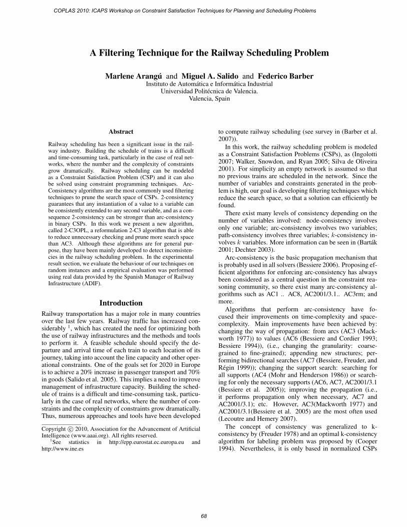
A Filtering Technique for the Railway Scheduling Problem

Marlene Arangu and Miguel A. Salido and Federico BarberInstituto de Automatica e Informatica Industrial

Universidad Politecnica de Valencia.Valencia, Spain

Abstract

Railway scheduling has been a significant issue in the rail-way industry. Building the schedule of trains is a difficultand time-consuming task, particularly in the case of real net-works, where the number and the complexity of constraintsgrow dramatically. Railway scheduling can be modeledas a Constraint Satisfaction Problem (CSP) and it can alsobe solved using constraint programming techniques. Arc-Consistency algorithms are the most commonly used filteringtechniques to prune the search space of CSPs. 2-consistencyguarantees that any instantiation of a value to a variable canbe consistently extended to any second variable, and as a con-sequence 2-consistency can be stronger than arc-consistencyin binary CSPs. In this work we present a new algorithm,called 2-C3OPL, a reformulation 2-C3 algorithm that is ableto reduce unnecessary checking and prune more search spacethan AC3. Although these algorithms are for general pur-pose, thay have been mainly developed to detect inconsisten-cies in the railway scheduling problem. In the experimentalresult section, we evaluate the behaviour of our techniques onrandom instances and a empirical evaluation was performedusing real data provided by the Spanish Manager of RailwayInfrastructure (ADIF).

IntroductionRailway transportation has a major role in many countriesover the last few years. Railway traffic has increased con-siderably 1, which has created the need for optimizing boththe use of railway infrastructures and the methods and toolsto perform it. A feasible schedule should specify the de-parture and arrival time of each train to each location of itsjourney, taking into account the line capacity and other oper-ational constraints. One of the goals set for 2020 in Europeis to achieve a 20% increase in passenger transport and 70%in goods (Salido et al. 2005). This implies a need to improvemanagement of infrastructure capacity. Building the sched-ule of trains is a difficult and time-consuming task, particu-larly in the case of real networks, where the number of con-straints and the complexity of constraints grow dramatically.Thus, numerous approaches and tools have been developed


1See statistics in http://epp.eurostat.ec.europa.eu andhttp://www.ine.es

to compute railway scheduling (see survey in (Barber et al.2007)).

In this work, the railway scheduling problem is modeledas a Constraint Satisfaction Problems (CSPs), as (Ingolotti2007; Walker, Snowdon, and Ryan 2005; Silva de Oliveira2001). For simplicity an empty network is assumed so thatno previous trains are scheduled in the network. Since thenumber of variables and constraints generated in the prob-lem is high, our goal is developing filtering techniques whichreduce the search space, so that a solution can efficiently befound.

There exist many levels of consistency depending on thenumber of variables involved: node-consistency involvesonly one variable; arc-consistency involves two variables;path-consistency involves three variables; k-consistency in-volves k variables. More information can be seen in (Bartak2001; Dechter 2003).

Arc-consistency is the basic propagation mechanism thatis probably used in all solvers (Bessiere 2006). Proposing ef-ficient algorithms for enforcing arc-consistency has alwaysbeen considered as a central question in the constraint rea-soning community, so there exist many arc-consistency al-gorithms such as AC1 .. AC8, AC2001/3.1.. AC3rm; andmore.

Algorithms that perform arc-consistency have fo-cused their improvements on time-complexity and space-complexity. Main improvements have been achieved by:changing the way of propagation: from arcs (AC3 (Mack-worth 1977)) to values (AC6 (Bessiere and Cordier 1993;Bessiere 1994)), (i.e., changing the granularity: coarse-grained to fine-grained); appending new structures; per-forming bidirectional searches (AC7 (Bessiere, Freuder, andRegin 1999)); changing the support search: searching forall supports (AC4 (Mohr and Henderson 1986)) or search-ing for only the necessary supports (AC6, AC7, AC2001/3.1(Bessiere et al. 2005)); improving the propagation (i.e.,it performs propagation only when necessary, AC7 andAC2001/3.1); etc. However, AC3(Mackworth 1977) andAC2001/3.1(Bessiere et al. 2005) are the most often used(Lecoutre and Hemery 2007).

The concept of consistency was generalized to k-consistency by (Freuder 1978) and an optimal k-consistencyalgorithm for labeling problem was proposed by (Cooper1994). Nevertheless, it is only based in normalized CSPs


68

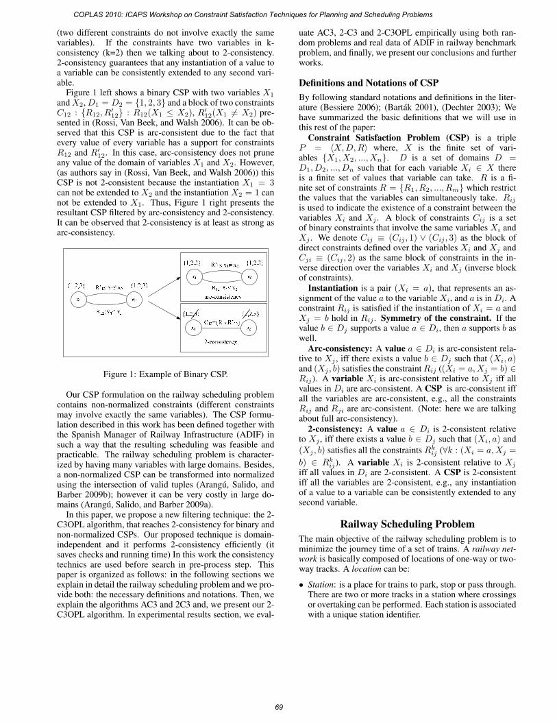
(two different constraints do not involve exactly the samevariables). If the constraints have two variables in k-consistency (k=2) then we talking about to 2-consistency.2-consistency guarantees that any instantiation of a value toa variable can be consistently extended to any second vari-able.

Figure 1 left shows a binary CSP with two variables X1

andX2,D1 = D2 = {1, 2, 3} and a block of two constraintsC12 : {R12, R

′12} : R12(X1 ≤ X2), R′

12(X1 �= X2) pre-sented in (Rossi, Van Beek, and Walsh 2006). It can be ob-served that this CSP is arc-consistent due to the fact thatevery value of every variable has a support for constraintsR12 and R′

12. In this case, arc-consistency does not pruneany value of the domain of variables X1 and X2. However,(as authors say in (Rossi, Van Beek, and Walsh 2006)) thisCSP is not 2-consistent because the instantiation X1 = 3can not be extended to X2 and the instantiation X2 = 1 cannot be extended to X1. Thus, Figure 1 right presents theresultant CSP filtered by arc-consistency and 2-consistency.It can be observed that 2-consistency is at least as strong asarc-consistency.

Figure 1: Example of Binary CSP.

Our CSP formulation on the railway scheduling problemcontains non-normalized constraints (different constraintsmay involve exactly the same variables). The CSP formu-lation described in this work has been defined together withthe Spanish Manager of Railway Infrastructure (ADIF) insuch a way that the resulting scheduling was feasible andpracticable. The railway scheduling problem is character-ized by having many variables with large domains. Besides,a non-normalized CSP can be transformed into normalizedusing the intersection of valid tuples (Arangu, Salido, andBarber 2009b); however it can be very costly in large do-mains (Arangu, Salido, and Barber 2009a).

In this paper, we propose a new filtering technique: the 2-C3OPL algorithm, that reaches 2-consistency for binary andnon-normalized CSPs. Our proposed technique is domain-independent and it performs 2-consistency efficiently (itsaves checks and running time) In this work the consistencytechnics are used before search in pre-process step. Thispaper is organized as follows: in the following sections weexplain in detail the railway scheduling problem and we pro-vide both: the necessary definitions and notations. Then, weexplain the algorithms AC3 and 2C3 and, we present our 2-C3OPL algorithm. In experimental results section, we eval-

uate AC3, 2-C3 and 2-C3OPL empirically using both ran-dom problems and real data of ADIF in railway benchmarkproblem, and finally, we present our conclusions and furtherworks.

Definitions and Notations of CSPBy following standard notations and definitions in the liter-ature (Bessiere 2006); (Bartak 2001), (Dechter 2003); Wehave summarized the basic definitions that we will use inthis rest of the paper:

Constraint Satisfaction Problem (CSP) is a tripleP = 〈X,D,R〉 where, X is the finite set of vari-ables {X1, X2, ..., Xn}. D is a set of domains D =D1, D2, ..., Dn such that for each variable Xi ∈ X thereis a finite set of values that variable can take. R is a fi-nite set of constraints R = {R1, R2, ..., Rm} which restrictthe values that the variables can simultaneously take. Rijis used to indicate the existence of a constraint between thevariables Xi and Xj . A block of constraints Cij is a setof binary constraints that involve the same variables Xi andXj . We denote Cij ≡ (Cij , 1) ∨ (Cij , 3) as the block ofdirect constraints defined over the variables Xi and Xj andCji ≡ (Cij , 2) as the same block of constraints in the in-verse direction over the variables Xi and Xj (inverse blockof constraints).

Instantiation is a pair (Xi = a), that represents an as-signment of the value a to the variable Xi, and a is in Di. Aconstraint Rij is satisfied if the instantiation of Xi = a andXj = b hold in Rij . Symmetry of the constraint. If thevalue b ∈ Dj supports a value a ∈ Di, then a supports b aswell.

Arc-consistency: A value a ∈ Di is arc-consistent rela-tive to Xj , iff there exists a value b ∈ Dj such that (Xi, a)and (Xj , b) satisfies the constraintRij ((Xi = a,Xj = b) ∈Rij). A variable Xi is arc-consistent relative to Xj iff allvalues in Di are arc-consistent. A CSP is arc-consistent iffall the variables are arc-consistent, e.g., all the constraintsRij and Rji are arc-consistent. (Note: here we are talkingabout full arc-consistency).

2-consistency: A value a ∈ Di is 2-consistent relativeto Xj , iff there exists a value b ∈ Dj such that (Xi, a) and

(Xj , b) satisfies all the constraints Rkij (∀k : (Xi = a,Xj =b) ∈ Rkij). A variable Xi is 2-consistent relative to Xj

iff all values in Di are 2-consistent. A CSP is 2-consistentiff all the variables are 2-consistent, e.g., any instantiationof a value to a variable can be consistently extended to anysecond variable.

Railway Scheduling ProblemThe main objective of the railway scheduling problem is tominimize the journey time of a set of trains. A railway net-work is basically composed of locations of one-way or two-way tracks. A location can be:

• Station: is a place for trains to park, stop or pass through.There are two or more tracks in a station where crossingsor overtaking can be performed. Each station is associatedwith a unique station identifier.


69

• Halt: is a place for trains to stop, pass through, but notpark. Each halt is associated with a unique halt identifier.

• Junction: is a place where two different tracks fork. Thereis no stop time. Each junction is associated with a uniquejunction identifier.

On a rail network, the user needs to schedule the paths ofn trains going in one direction (up) and m trains going inthe opposite direction (down). These trains are of a giventype and a scheduling frequency is required. The type oftrains to be scheduled determines the time assigned for travelbetween two locations on the path. The path selected bythe user for a train trip determines which stations are usedand the stop time required at each station for commercialpurposes. In order to perform crossing in a section with aone-way track, one of the trains should wait in a station. Thisis called a technical stop. One of the trains is detoured fromthe main track so that the other train can cross or continue.

A running map contains information regarding the topol-ogy of the railways (stations, tracks, distances between sta-tions, traffic control features, etc.) and the schedules of thetrains that use this topology (arrival and departure times oftrains at each station, frequency, stops, crossing, overtaking,etc.). We assume that two connected locations have only oneline connecting them.

The Figure 2 shows a running map where the names ofthe stations are presented on the left side and the verticalline represents the number of tracks between stations (one-way or two-way). Horizontal dotted lines represent halts orjunctions, while solid lines represent stations. The objectiveis to obtain a correct and optimized running map taking intoaccount: (i) traffic rules, (ii) user requirements and (iii) therailway infrastructure topology.

Notation of railway scheduling problemThe notation used to describe the railway scheduling prob-lem is based on the works of (Ingolotti 2007; Tormos et al.2008). The notation is the following:

• T : finite set of trains t considered in the problem. T ={t1, t2, ..., tk}. TD: set of trains traveling in the downdirection. TU : set of trains traveling in the up direction.Thus, T = TD ∪ TU and TD ∩ TU = ∅.

• L = {l0, l1, ..., lm}: railway line that is composed by anordered sequence of locations (stations, halts, junctions)that may be visited by trains t ∈ T . The contiguous lo-cations li and li+1 are linked by a single or double tracksection.

• Jt: journey of train t. It is described by an ordered se-quence of locations to be visited by a train t such that∀t ∈ T, ∃Jt : Jt ⊆ L. The journey Jt shows the or-der that is used by train t to visit a given set of locations.Thus, lt0 and ltnt

represent the fist and last location visitedby train t, respectively.

• Cti minimum time required for train t to perform commer-cial operations (such as boarding or leaving passengers) atstation i (commercial stop).

• Δti→(i+1): journey time for train t from location lti to

lt(i+1).

• F : Frequency of trains t ∈ T considered in the problem.FD: Frequency of trains traveling in the down direction.FU : Frequency of of trains traveling in the up direction.

• λ: delay time allowed for train t with frequency F .

CSP formulation of railway schedulingproblem

A CSP formulation consists of the tuple 〈 X, D, R 〉, whereX is a set of variables, D is a set of domains and R is a setof binary constraints.

VariablesEach train travelling in each location will generate two

different variables (arrival and departure time):

• depti departure time of train t ∈ T from the location i,where i ∈ Jt \ {ltnt

}.

• arrti arrival time of train t ∈ T to the location i, wherei ∈ Jt \ {lt0}.

DomainsThe domain of each variable (depti or arrti) is an interval

[minV ,maxV ], where minV ≥ 0 and maxV > minV .This interval is obtained from data of ADIF, according tothe journey.

ConstraintsThere are three groups of scheduling rules in our railway

system: traffic rules, user requirements rules and topologicalrules. A valid running map must satisfy and optimize theabove rules. These scheduling rules can be modeled usingthe following constraints:

1. Traffic rules guarantee crossing and overtaking opera-tions. The main constraints to take into account are:

• Crossing constraint: Any two trains going in oppositedirections must not simultaneously use the same one-

way track: dept′i+1 > arrti+1 ∨ depti > arrt

′i .

• Expedition time constraint. There exists a given timeto put a detoured train back on the main track and exit

from a station: |dept′l − arrtl | ≥ Et, where Et is theexpedition time specified for t.

• Reception time constraint. There exists a given time todetour a train from the main track so that crossing or

overtaking can be performed: arrt′l ≥ arrtl → arrt

′l −

arrtl ≥ Recept, where Recept is the reception timespecified for the train that arrives to l first.

• Journey Time constraint. arrti+1 = depti + Δti→(i+1).

For each train t and each track section, a Journey time isgiven by Δt

i→(i+1), which represents the time the train

t should employ to go from location lti to location lti+1.

2. User Requirements: The main constraints due to user re-quirements are:

• Number of trains going in each direction n (down) andm (up) to be scheduled. T = TD ∪ TU , where:


70

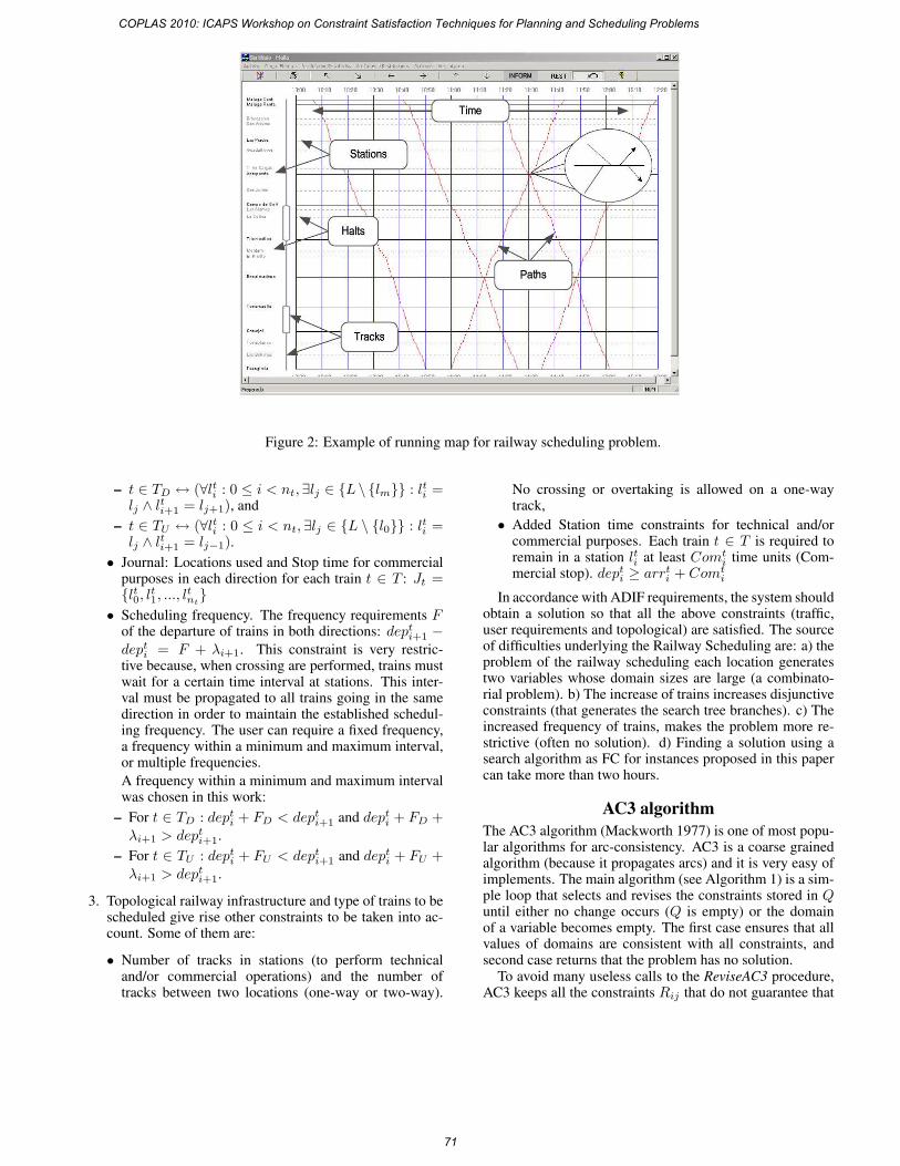
Figure 2: Example of running map for railway scheduling problem.

– t ∈ TD ↔ (∀lti : 0 ≤ i < nt,∃lj ∈ {L \ {lm}} : lti =lj ∧ lti+1 = lj+1), and

– t ∈ TU ↔ (∀lti : 0 ≤ i < nt,∃lj ∈ {L \ {l0}} : lti =lj ∧ lti+1 = lj−1).

• Journal: Locations used and Stop time for commercialpurposes in each direction for each train t ∈ T : Jt ={lt0, lt1, ..., ltnt

}• Scheduling frequency. The frequency requirements F

of the departure of trains in both directions: depti+1 −depti = F + λi+1. This constraint is very restric-tive because, when crossing are performed, trains mustwait for a certain time interval at stations. This inter-val must be propagated to all trains going in the samedirection in order to maintain the established schedul-ing frequency. The user can require a fixed frequency,a frequency within a minimum and maximum interval,or multiple frequencies.

A frequency within a minimum and maximum intervalwas chosen in this work:

– For t ∈ TD : depti + FD < depti+1 and depti + FD +λi+1 > depti+1.

– For t ∈ TU : depti + FU < depti+1 and depti + FU +λi+1 > depti+1.

3. Topological railway infrastructure and type of trains to bescheduled give rise other constraints to be taken into ac-count. Some of them are:

• Number of tracks in stations (to perform technicaland/or commercial operations) and the number oftracks between two locations (one-way or two-way).

No crossing or overtaking is allowed on a one-waytrack,

• Added Station time constraints for technical and/orcommercial purposes. Each train t ∈ T is required toremain in a station lti at least Comt

i time units (Com-mercial stop). depti ≥ arrti + Comt

i

In accordance with ADIF requirements, the system shouldobtain a solution so that all the above constraints (traffic,user requirements and topological) are satisfied. The sourceof difficulties underlying the Railway Scheduling are: a) theproblem of the railway scheduling each location generatestwo variables whose domain sizes are large (a combinato-rial problem). b) The increase of trains increases disjunctiveconstraints (that generates the search tree branches). c) Theincreased frequency of trains, makes the problem more re-strictive (often no solution). d) Finding a solution using asearch algorithm as FC for instances proposed in this papercan take more than two hours.

AC3 algorithmThe AC3 algorithm (Mackworth 1977) is one of most popu-lar algorithms for arc-consistency. AC3 is a coarse grainedalgorithm (because it propagates arcs) and it is very easy ofimplements. The main algorithm (see Algorithm 1) is a sim-ple loop that selects and revises the constraints stored in Quntil either no change occurs (Q is empty) or the domainof a variable becomes empty. The first case ensures that allvalues of domains are consistent with all constraints, andsecond case returns that the problem has no solution.

To avoid many useless calls to the ReviseAC3 procedure,AC3 keeps all the constraints Rij that do not guarantee that


71

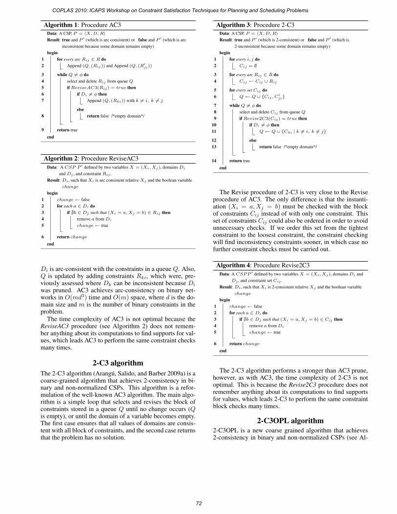
Algorithm 1: Procedure AC3

Data: A CSP, P = 〈X,D,R〉Result: true and P ′ (which is arc consistent) or false and P ′ (which is arc

inconsistent because some domain remains empty)

beginfor every arc Rij ∈ R do1

Append (Q, (Rij)) and Append (Q, (R′ji))2

while Q �= φ do3select and delete Rij from queue Q4ifReviseAC3(Rij) = true then5

ifDi �= φ then6Append (Q, (Rki)) with k �= i, k �= j7

elsereturn false /*empty domain*/8

return true9end

Algorithm 2: Procedure ReviseAC3

Data: A CSP P ′ defined by two variables X = (Xi, Xj), domains Di

andDj , and constraint Rij .

Result: Di, such that Xi is arc consistent relative Xj and the boolean variable

change

beginchange ← false1for each a ∈ Di do2

if �b ∈ Dj such that (Xi = a,Xj = b) ∈ Rij then3remove a fromDi4change ← true5

return change6end

Di is arc-consistent with the constraints in a queue Q. Also,Q is updated by adding constraints Rki, which were, pre-viously assessed where Dk can be inconsistent because Di

was pruned. AC3 achieves arc-consistency on binary net-works in O(md3) time and O(m) space, where d is the do-main size and m is the number of binary constraints in theproblem.

The time complexity of AC3 is not optimal because theReviseAC3 procedure (see Algorithm 2) does not remem-ber anything about its computations to find supports for val-ues, which leads AC3 to perform the same constraint checksmany times.

2-C3 algorithmThe 2-C3 algorithm (Arangu, Salido, and Barber 2009a) is acoarse-grained algorithm that achieves 2-consistency in bi-nary and non-normalized CSPs. This algorithm is a refor-mulation of the well-known AC3 algorithm. The main algo-rithm is a simple loop that selects and revises the block ofconstraints stored in a queue Q until no change occurs (Qis empty), or until the domain of a variable becomes empty.The first case ensures that all values of domains are consis-tent with all block of constraints, and the second case returnsthat the problem has no solution.

Algorithm 3: Procedure 2-C3

Data: A CSP, P = 〈X,D,R〉Result: true and P ′ (which is 2-consistent) or false and P ′ (which is

2-inconsistent because some domain remains empty)

beginfor every i, j do1

Cij = ∅2

for every arcRij ∈ R do3Cij ← Cij ∪ Rij4

for every set Cij do5Q ← Q ∪ {Cij , C

′ji}6

whileQ �= φ do7select and delete Cij from queue Q8ifRevise2C3(Cij) = true then9

ifDi �= φ then10Q ← Q ∪ {Cki | k �= i, k �= j}11

else12return false /*empty domain*/13

return true14end

The Revise procedure of 2-C3 is very close to the Reviseprocedure of AC3. The only difference is that the instanti-ation (Xi = a,Xj = b) must be checked with the blockof constraints Cij instead of with only one constraint. Thisset of constraints Cij could also be ordered in order to avoidunnecessary checks. If we order this set from the tightestconstraint to the loosest constraint, the constraint checkingwill find inconsistency constraints sooner, in which case nofurther constraint checks must be carried out.

Algorithm 4: Procedure Revise2C3

Data: A CSPP ′ defined by two variables X = (Xi, Xj), domains Di and

Dj , and constraint set Cij .

Result: Di, such thatXi is 2-consistent relative Xj and the boolean variable

change

beginchange ← false1for each a ∈ Di do2

if �b ∈ Dj such that (Xi = a,Xj = b) ∈ Cij then3remove a fromDi4change ← true5

return change6end

The 2-C3 algorithm performs a stronger than AC3 prune,however, as with AC3, the time complexity of 2-C3 is notoptimal. This is because the Revise2C3 procedure does notremember anything about its computations to find supportsfor values, which leads 2-C3 to perform the same constraintblock checks many times.

2-C3OPL algorithm2-C3OPL is a new coarse grained algorithm that achieves2-consistency in binary and non-normalized CSPs (see Al-


72

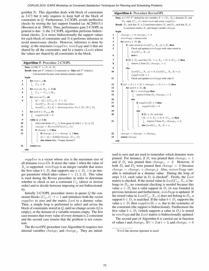
gorithm 5). This algorithm deals with block of constraintsas 2-C3 but it only requires to keep half of the block ofconstraints in Q. Furthermore, 2-C3OPL avoids ineffectivechecks by storing the last support founded (as AC2001/3.1(Bessiere et al. 2005)). Thus, performance gain 2-C3OPL ingeneral is due: 1) the 2-C3OPL algorithm performs bidirec-tional checks; 2) it stores bidirectionally the support valuesfor each block of constraints and 3) it performs inference toavoid unnecessary checks. However, inference is done byusing: a) the structures (suppInv, minSupp and t) that areshared by all the constraints, and b) a matrix (Last) wherethe values are shared by all constraints in the block.

Algorithm 5: Procedure 2-C3OPL

Data: A CSP, P = 〈X,D,R〉Result: true and P ′ (which is 2-consistent) or false and P ′ (which is

2-inconsistent because some domain remains empty)

beginfor every i, j do1

Cij = ∅2

for every arc Rij ∈ R do3Cij ← Cij ∪ Rij4

for every set Cij do5Q ← Q ∪ {(Cij , t) : t = 1}6Last[Cij , Xi, a] = dummyvalue;

Last[Cij , Xj, b] = dummyvalue; ∀a ∈ Di; ∀b ∈ Dj

for each d ∈ Dmax do7suppInv[d] = 08

while Q �= ∅ do9select and delete (Cij , t) from queue Q with t = {1, 2, 3}10change = ReviseOPL((Cij , t))11if change > 0 then12

If change ≥ 1 ∧ change ≤ 3 then13Q ← Q ∪ AddQ(change, (Cij , t))

else return false /*empty domain*/

return true14end

suppInv is a vector whose size is the maximum size ofall domains (maxD). It stores the value 1 when the value ofXj is supported. minSupp is an integer variable that storesthe first value b ∈ Dj that supports any a ∈ Di. t is an inte-ger parameter which takes values t = {1, 2, 3}. This valueis used during the Revise procedure in order to determinewhether to check or not a constraint Cij (direct or inverseorder) and to decide between imposing or not bidirectional-ity.

Initially 2-C3OPL procedure stores in queue Q the con-straint blocks (Cij , t) : t = 1 and initializes both the vectorsuppInv to zero and the matrix Last to a dummy value.Then, a simple loop is performed to select and revise theblock of constraints stored inQ, until no change occurs (Q isempty), or the domain of a variable remains empty. The firstcase ensures that every value of every domain is 2-consistentand the second case returns that the problem is not consis-tent.

The ReviseOPL procedure (see Algorithm 6) requires twointernal variables changei and changej . They are initial-

Algorithm 6: Procedure ReviseOPL

Data: A CSP P ′ defined by two variables X = (Xi, Xj), domainsDi and

Dj , tuple (Cij , t), vector Last and vector suppInv.

Result: Di, such thatXi is 2-consistent relative Xj andDj , such that Xj is

2-consistent relative Xi and integer variable change

beginchangei = 0; changej = 01minSupp =dummyvalue2for each a ∈ Di do3

if value stored in Last[Cij , Xi, a] ∈ Dj then4Check and update(minSupp) with value stored in5Last[Cij , Xi, a]

next a6

if �b ∈ Dj such that (Xi = a,Xj = b) ∈ (Cij , t) then7remove a fromDi; changei = 18

else9Last[Cij , Xi, a] = b; Last[Cij , Xj , b] = a;10suppInv[b] = 1

Check and update(minSupp) with value b11

if ([(t = 2 ∨ t = 3) ∧ changei = 1] ∨ t = 1) then12for each b ∈ Dj do13

if b < minSupp then14remove b fromDj ; changej = 215

else16if suppInv[b] > 0 then17

suppInv[b] = 018

else19if �a ∈ Di such that20(Xi = a,Xj = b) ∈ (Cij , t) then

remove b fromDj ; changej = 221

else Last[Cij , Xj , b] = a

change = changei + changej22return change23

end

ized to zero and are used to remember which domains werepruned. For instance, if Di was pruned then changei = 1and if Dj was pruned then changej = 2. However, ifboth Di and Dj were pruned then change = 3 (becausechange = changei + changej). Also, minorSupp vari-able is initialized in a dummy value. During the loop ofsteps 3-11, each value in Di is checked2. Firstly, the Lastmatrix is checked. If the stored value in Last[Cij , Xi, a] be-longs to Dj , no constraint checking is needed because thisvalue a ∈ Di has a valid support in Dj (it was founded inprevious iteration) and furthermore,minSupp is updated. Ifthe stored value in Last[Cij , Xi, a] does not belong toDj , asupport b ∈ Dj is searched. If the value b ∈ Dj supports thevalue a ∈ Di then suppInv[b] = a, due to the symmetry ofthe constraint (the support is bidirectional). Furthermore thefirst value b ∈ Dj (which supports a value in Di) is storedin minSupp and the Last matrix is bidirectionally updated.

The second part of Algorithm 6 is carried out in functionof values t and changei. If t = 2 or t = 3, and changei = 0

2if t=2 the inverse operator is used


73

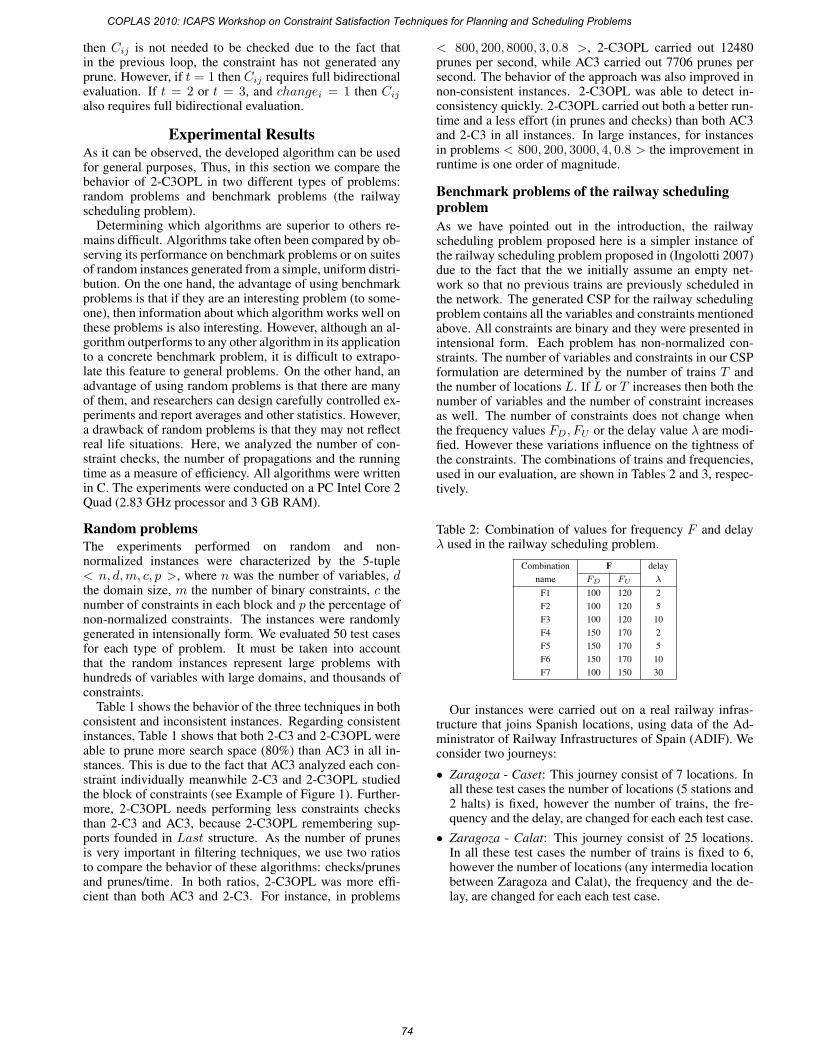
then Cij is not needed to be checked due to the fact thatin the previous loop, the constraint has not generated anyprune. However, if t = 1 then Cij requires full bidirectionalevaluation. If t = 2 or t = 3, and changei = 1 then Cijalso requires full bidirectional evaluation.

Experimental ResultsAs it can be observed, the developed algorithm can be usedfor general purposes, Thus, in this section we compare thebehavior of 2-C3OPL in two different types of problems:random problems and benchmark problems (the railwayscheduling problem).

Determining which algorithms are superior to others re-mains difficult. Algorithms take often been compared by ob-serving its performance on benchmark problems or on suitesof random instances generated from a simple, uniform distri-bution. On the one hand, the advantage of using benchmarkproblems is that if they are an interesting problem (to some-one), then information about which algorithm works well onthese problems is also interesting. However, although an al-gorithm outperforms to any other algorithm in its applicationto a concrete benchmark problem, it is difficult to extrapo-late this feature to general problems. On the other hand, anadvantage of using random problems is that there are manyof them, and researchers can design carefully controlled ex-periments and report averages and other statistics. However,a drawback of random problems is that they may not reflectreal life situations. Here, we analyzed the number of con-straint checks, the number of propagations and the runningtime as a measure of efficiency. All algorithms were writtenin C. The experiments were conducted on a PC Intel Core 2Quad (2.83 GHz processor and 3 GB RAM).

Random problemsThe experiments performed on random and non-normalized instances were characterized by the 5-tuple< n, d,m, c, p >, where n was the number of variables, dthe domain size, m the number of binary constraints, c thenumber of constraints in each block and p the percentage ofnon-normalized constraints. The instances were randomlygenerated in intensionally form. We evaluated 50 test casesfor each type of problem. It must be taken into accountthat the random instances represent large problems withhundreds of variables with large domains, and thousands ofconstraints.

Table 1 shows the behavior of the three techniques in bothconsistent and inconsistent instances. Regarding consistentinstances, Table 1 shows that both 2-C3 and 2-C3OPL wereable to prune more search space (80%) than AC3 in all in-stances. This is due to the fact that AC3 analyzed each con-straint individually meanwhile 2-C3 and 2-C3OPL studiedthe block of constraints (see Example of Figure 1). Further-more, 2-C3OPL needs performing less constraints checksthan 2-C3 and AC3, because 2-C3OPL remembering sup-ports founded in Last structure. As the number of prunesis very important in filtering techniques, we use two ratiosto compare the behavior of these algorithms: checks/prunesand prunes/time. In both ratios, 2-C3OPL was more effi-cient than both AC3 and 2-C3. For instance, in problems

< 800, 200, 8000, 3, 0.8 >, 2-C3OPL carried out 12480prunes per second, while AC3 carried out 7706 prunes persecond. The behavior of the approach was also improved innon-consistent instances. 2-C3OPL was able to detect in-consistency quickly. 2-C3OPL carried out both a better run-time and a less effort (in prunes and checks) than both AC3and 2-C3 in all instances. In large instances, for instancesin problems < 800, 200, 3000, 4, 0.8 > the improvement inruntime is one order of magnitude.

Benchmark problems of the railway schedulingproblemAs we have pointed out in the introduction, the railwayscheduling problem proposed here is a simpler instance ofthe railway scheduling problem proposed in (Ingolotti 2007)due to the fact that the we initially assume an empty net-work so that no previous trains are previously scheduled inthe network. The generated CSP for the railway schedulingproblem contains all the variables and constraints mentionedabove. All constraints are binary and they were presented inintensional form. Each problem has non-normalized con-straints. The number of variables and constraints in our CSPformulation are determined by the number of trains T andthe number of locations L. If L or T increases then both thenumber of variables and the number of constraint increasesas well. The number of constraints does not change whenthe frequency values FD, FU or the delay value λ are modi-fied. However these variations influence on the tightness ofthe constraints. The combinations of trains and frequencies,used in our evaluation, are shown in Tables 2 and 3, respec-tively.

Table 2: Combination of values for frequency F and delayλ used in the railway scheduling problem.

Combination F delay

name FD FU λ

F1 100 120 2

F2 100 120 5

F3 100 120 10

F4 150 170 2

F5 150 170 5

F6 150 170 10

F7 100 150 30

Our instances were carried out on a real railway infras-tructure that joins Spanish locations, using data of the Ad-ministrator of Railway Infrastructures of Spain (ADIF). Weconsider two journeys:

• Zaragoza - Caset: This journey consist of 7 locations. Inall these test cases the number of locations (5 stations and2 halts) is fixed, however the number of trains, the fre-quency and the delay, are changed for each each test case.

• Zaragoza - Calat: This journey consist of 25 locations.In all these test cases the number of trains is fixed to 6,however the number of locations (any intermedia locationbetween Zaragoza and Calat), the frequency and the de-lay, are changed for each each test case.


74

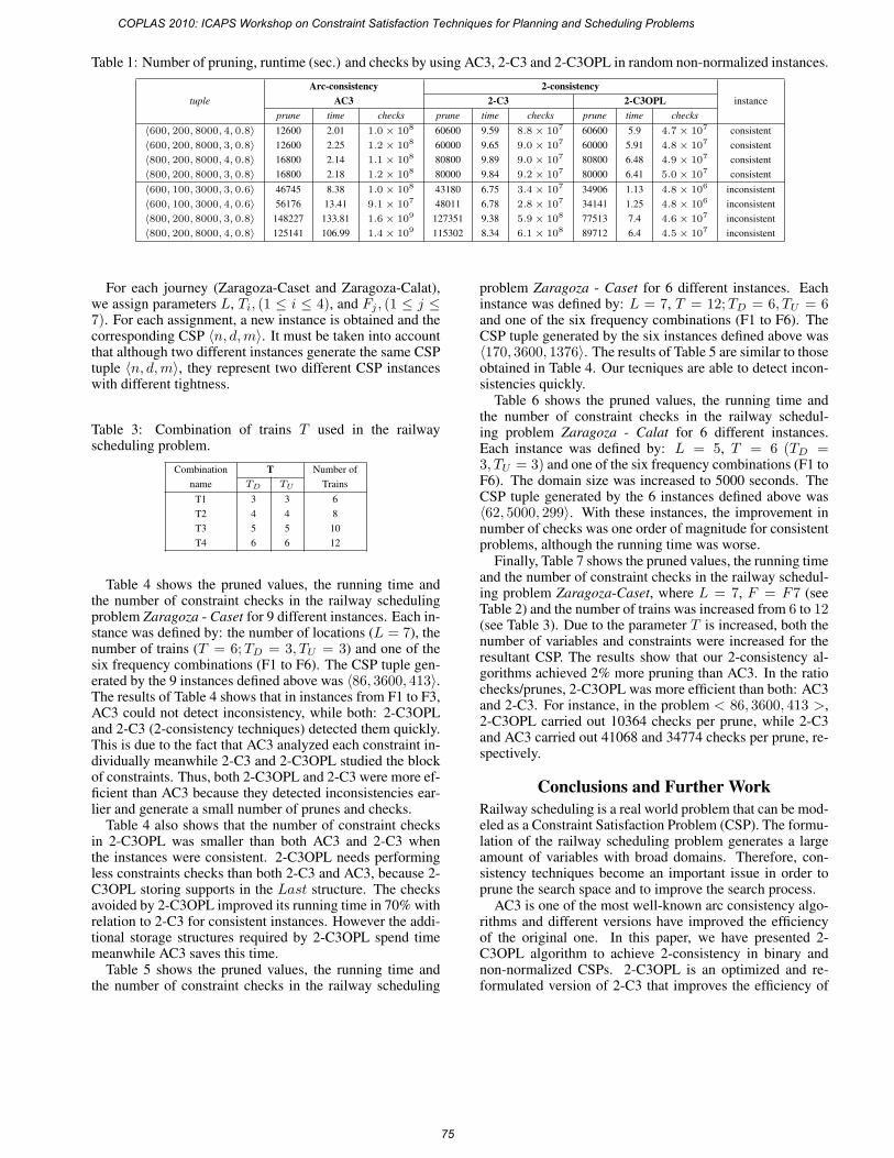
Table 1: Number of pruning, runtime (sec.) and checks by using AC3, 2-C3 and 2-C3OPL in random non-normalized instances.

Arc-consistency 2-consistencytuple AC3 2-C3 2-C3OPL instance

prune time checks prune time checks prune time checks〈600, 200, 8000, 4, 0.8〉 12600 2.01 1.0 × 108 60600 9.59 8.8 × 107 60600 5.9 4.7 × 107 consistent

〈600, 200, 8000, 3, 0.8〉 12600 2.25 1.2 × 108 60000 9.65 9.0 × 107 60000 5.91 4.8 × 107 consistent

〈800, 200, 8000, 4, 0.8〉 16800 2.14 1.1 × 108 80800 9.89 9.0 × 107 80800 6.48 4.9 × 107 consistent

〈800, 200, 8000, 3, 0.8〉 16800 2.18 1.2 × 108 80000 9.84 9.2 × 107 80000 6.41 5.0 × 107 consistent

〈600, 100, 3000, 3, 0.6〉 46745 8.38 1.0 × 108 43180 6.75 3.4 × 107 34906 1.13 4.8 × 106 inconsistent

〈600, 100, 3000, 4, 0.6〉 56176 13.41 9.1 × 107 48011 6.78 2.8 × 107 34141 1.25 4.8 × 106 inconsistent

〈800, 200, 8000, 3, 0.8〉 148227 133.81 1.6 × 109 127351 9.38 5.9 × 108 77513 7.4 4.6 × 107 inconsistent

〈800, 200, 8000, 4, 0.8〉 125141 106.99 1.4 × 109 115302 8.34 6.1 × 108 89712 6.4 4.5 × 107 inconsistent

For each journey (Zaragoza-Caset and Zaragoza-Calat),we assign parameters L, Ti, (1 ≤ i ≤ 4), and Fj , (1 ≤ j ≤7). For each assignment, a new instance is obtained and thecorresponding CSP 〈n, d,m〉. It must be taken into accountthat although two different instances generate the same CSPtuple 〈n, d,m〉, they represent two different CSP instanceswith different tightness.

Table 3: Combination of trains T used in the railwayscheduling problem.

Combination T Number of

name TD TU Trains

T1 3 3 6

T2 4 4 8

T3 5 5 10

T4 6 6 12

Table 4 shows the pruned values, the running time andthe number of constraint checks in the railway schedulingproblem Zaragoza - Caset for 9 different instances. Each in-stance was defined by: the number of locations (L = 7), thenumber of trains (T = 6;TD = 3, TU = 3) and one of thesix frequency combinations (F1 to F6). The CSP tuple gen-erated by the 9 instances defined above was 〈86, 3600, 413〉.The results of Table 4 shows that in instances from F1 to F3,AC3 could not detect inconsistency, while both: 2-C3OPLand 2-C3 (2-consistency techniques) detected them quickly.This is due to the fact that AC3 analyzed each constraint in-dividually meanwhile 2-C3 and 2-C3OPL studied the blockof constraints. Thus, both 2-C3OPL and 2-C3 were more ef-ficient than AC3 because they detected inconsistencies ear-lier and generate a small number of prunes and checks.

Table 4 also shows that the number of constraint checksin 2-C3OPL was smaller than both AC3 and 2-C3 whenthe instances were consistent. 2-C3OPL needs performingless constraints checks than both 2-C3 and AC3, because 2-C3OPL storing supports in the Last structure. The checksavoided by 2-C3OPL improved its running time in 70% withrelation to 2-C3 for consistent instances. However the addi-tional storage structures required by 2-C3OPL spend timemeanwhile AC3 saves this time.

Table 5 shows the pruned values, the running time andthe number of constraint checks in the railway scheduling

problem Zaragoza - Caset for 6 different instances. Eachinstance was defined by: L = 7, T = 12;TD = 6, TU = 6and one of the six frequency combinations (F1 to F6). TheCSP tuple generated by the six instances defined above was〈170, 3600, 1376〉. The results of Table 5 are similar to thoseobtained in Table 4. Our tecniques are able to detect incon-sistencies quickly.

Table 6 shows the pruned values, the running time andthe number of constraint checks in the railway schedul-ing problem Zaragoza - Calat for 6 different instances.Each instance was defined by: L = 5, T = 6 (TD =3, TU = 3) and one of the six frequency combinations (F1 toF6). The domain size was increased to 5000 seconds. TheCSP tuple generated by the 6 instances defined above was〈62, 5000, 299〉. With these instances, the improvement innumber of checks was one order of magnitude for consistentproblems, although the running time was worse.

Finally, Table 7 shows the pruned values, the running timeand the number of constraint checks in the railway schedul-ing problem Zaragoza-Caset, where L = 7, F = F7 (seeTable 2) and the number of trains was increased from 6 to 12(see Table 3). Due to the parameter T is increased, both thenumber of variables and constraints were increased for theresultant CSP. The results show that our 2-consistency al-gorithms achieved 2% more pruning than AC3. In the ratiochecks/prunes, 2-C3OPL was more efficient than both: AC3and 2-C3. For instance, in the problem < 86, 3600, 413 >,2-C3OPL carried out 10364 checks per prune, while 2-C3and AC3 carried out 41068 and 34774 checks per prune, re-spectively.

Conclusions and Further WorkRailway scheduling is a real world problem that can be mod-eled as a Constraint Satisfaction Problem (CSP). The formu-lation of the railway scheduling problem generates a largeamount of variables with broad domains. Therefore, con-sistency techniques become an important issue in order toprune the search space and to improve the search process.

AC3 is one of the most well-known arc consistency algo-rithms and different versions have improved the efficiencyof the original one. In this paper, we have presented 2-C3OPL algorithm to achieve 2-consistency in binary andnon-normalized CSPs. 2-C3OPL is an optimized and re-formulated version of 2-C3 that improves the efficiency of


75

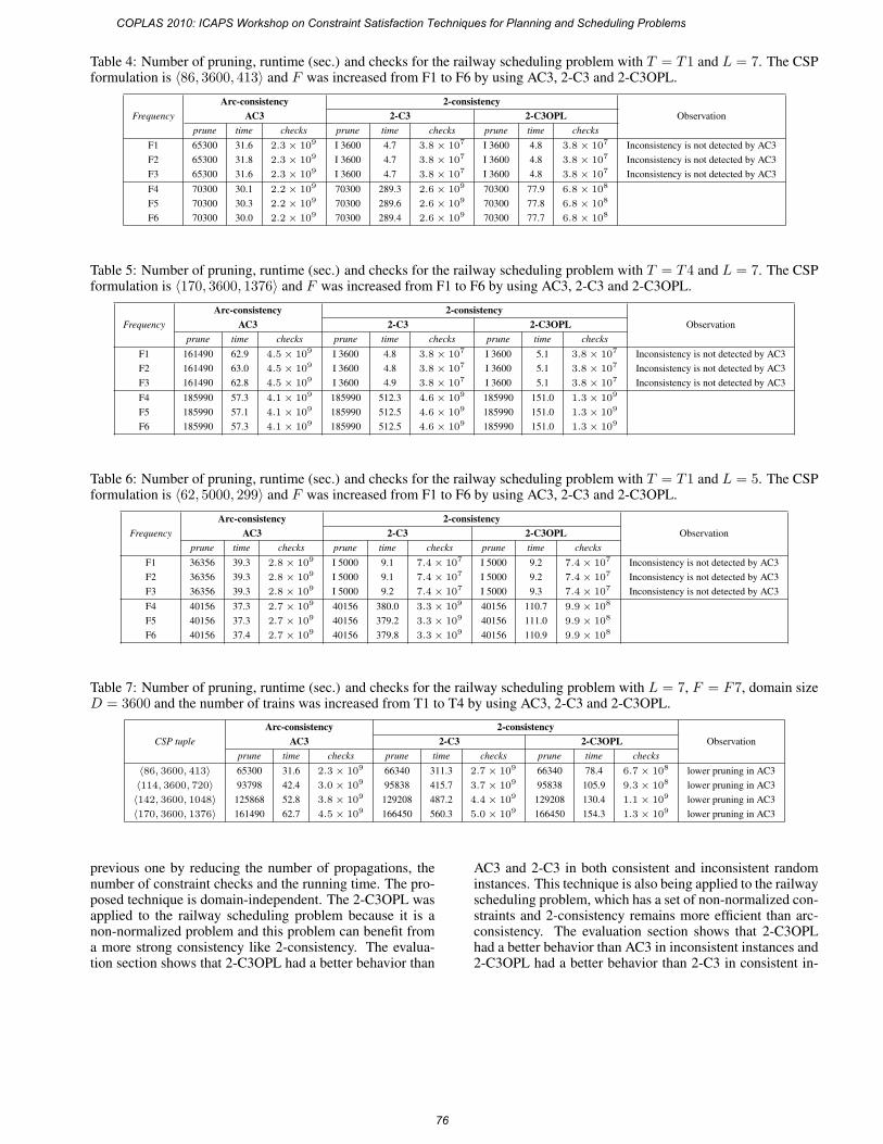
Table 4: Number of pruning, runtime (sec.) and checks for the railway scheduling problem with T = T1 and L = 7. The CSPformulation is 〈86, 3600, 413〉 and F was increased from F1 to F6 by using AC3, 2-C3 and 2-C3OPL.

Arc-consistency 2-consistencyFrequency AC3 2-C3 2-C3OPL Observation

prune time checks prune time checks prune time checksF1 65300 31.6 2.3 × 109 I 3600 4.7 3.8 × 107 I 3600 4.8 3.8 × 107 Inconsistency is not detected by AC3

F2 65300 31.8 2.3 × 109 I 3600 4.7 3.8 × 107 I 3600 4.8 3.8 × 107 Inconsistency is not detected by AC3


F4 70300 30.1 2.2 × 109 70300 289.3 2.6 × 109 70300 77.9 6.8 × 108

F5 70300 30.3 2.2 × 109 70300 289.6 2.6 × 109 70300 77.8 6.8 × 108

F6 70300 30.0 2.2 × 109 70300 289.4 2.6 × 109 70300 77.7 6.8 × 108






F4 185990 57.3 4.1 × 109 185990 512.3 4.6 × 109 185990 151.0 1.3 × 109

F5 185990 57.1 4.1 × 109 185990 512.5 4.6 × 109 185990 151.0 1.3 × 109

F6 185990 57.3 4.1 × 109 185990 512.5 4.6 × 109 185990 151.0 1.3 × 109






F4 40156 37.3 2.7 × 109 40156 380.0 3.3 × 109 40156 110.7 9.9 × 108

F5 40156 37.3 2.7 × 109 40156 379.2 3.3 × 109 40156 111.0 9.9 × 108

F6 40156 37.4 2.7 × 109 40156 379.8 3.3 × 109 40156 110.9 9.9 × 108

Table 7: Number of pruning, runtime (sec.) and checks for the railway scheduling problem with L = 7, F = F7, domain sizeD = 3600 and the number of trains was increased from T1 to T4 by using AC3, 2-C3 and 2-C3OPL.

Arc-consistency 2-consistencyCSP tuple AC3 2-C3 2-C3OPL Observation

prune time checks prune time checks prune time checks〈86, 3600, 413〉 65300 31.6 2.3 × 109 66340 311.3 2.7 × 109 66340 78.4 6.7 × 108 lower pruning in AC3

〈114, 3600, 720〉 93798 42.4 3.0 × 109 95838 415.7 3.7 × 109 95838 105.9 9.3 × 108 lower pruning in AC3



previous one by reducing the number of propagations, thenumber of constraint checks and the running time. The pro-posed technique is domain-independent. The 2-C3OPL wasapplied to the railway scheduling problem because it is anon-normalized problem and this problem can benefit froma more strong consistency like 2-consistency. The evalua-tion section shows that 2-C3OPL had a better behavior than

AC3 and 2-C3 in both consistent and inconsistent randominstances. This technique is also being applied to the railwayscheduling problem, which has a set of non-normalized con-straints and 2-consistency remains more efficient than arc-consistency. The evaluation section shows that 2-C3OPLhad a better behavior than AC3 in inconsistent instances and2-C3OPL had a better behavior than 2-C3 in consistent in-


76

stances. Furthermore, AC3 was unable to detect some in-consistencies (see evaluation section) while both 2-C3OPLand 2-C3 detected the inconsistency efficiently. Railway op-erators are very interesting on detecting inconsistencies inpreliminary/tentative timetables so that our techniques re-main useful to determine inconsistencies in the first steps ofa timetable generation. Also shows that the running timeis reduced up to 75% and the number of constraint checksis reduced up to 50% in relation to 2-C3 for consistent in-stances.

In further work, we will focus our attention to apply thesefiltering techniques to MAC2-C in order to improve the effi-ciency during search.

AcknowledgmentsThis work has been partially supported by the researchprojects TIN2007-67943-C02-01 (Min. de Educacion yCiencia, Spain-FEDER) and P19/08 (Min. de Fomento,Spain-FEDER)

ReferencesArangu, M.; Salido, M.; and Barber, F. 2009a. 2-C3: Fromarc-consistency to 2-consistency. In SARA 2009.

Arangu, M.; Salido, M.; and Barber, F. 2009b. Nor-malizando CSP no-normalizados: un enfoque hıbrido. InCAEPIA-TTIA 2009. Workshop on Planning, Schedulingand Constraint Satisfaction., 57–68.

Barber, F.; Abril, M.; Salido, M. A.; Ingolotti, L.; Tor-mos, P.; and Lova, A. 2007. Survey of automated sys-tems for railway management. Technical report, DSIC-II/01/07.UPV.

Bartak, R. 2001. Theory and practice of constraint propa-gation. In Figwer, J., ed., Proceedings of the 3rd Workshopon Constraint Programming in Decision and Control.Bessiere, C., and Cordier, M. 1993. Arc-consistency andarc-consistency again. In Proc. of the AAAI’93, 108–113.

Bessiere, C.; Regin, J. C.; Yap, R.; and Zhang, Y. 2005.An optimal coarse-grained arc-consistency algorithm. Ar-tificial Intelligence 165:165–185.

Bessiere, C.; Freuder, E.; and Regin, J. C. 1999. Usingconstraint metaknowledge to reduce arc consistency com-putation. Artificial Intelligence 107:125–148.

Bessiere, C. 1994. Arc-consistency and arc-consistencyagain. Artificial Intelligence 65:179–190.

Bessiere, C. 2006. Constraint propagation. Technical re-port, CNRS.

Cooper, M. 1994. An optimal k-consistency algorithm.Artificial Intelligence 41:89–95.

Dechter, R. 2003. Constraint Processing. Morgan Kauf-mann.

Freuder, E. 1978. Synthesizing constraint expressions.Communications of the ACM 21:958–966.

Ingolotti, L. 2007. Modelos y metodos para la opti-mizacion y eficiencia de la programacion de horarios fer-roviarios. Ph.D. Dissertation, Universidad Politecnica deValencia.

Lecoutre, C., and Hemery, F. 2007. A study of residualsupports in arc consistency. In proceedings IJCAI 2007,125–130.

Mackworth, A. K. 1977. Consistency in networks of rela-tions. Artificial Intelligence 8:99–118.

Mohr, R., and Henderson, T. 1986. Arc and path consis-tency revised. Artificial Intelligence 28:225–233.

Rossi, F.; Van Beek, P.; and Walsh, T. 2006. Handbook ofconstraint programming. Elsevier.

Salido, M.; Barber, F.; Abril, M.; Ingolotti, L.; Lova, A.;Tormos, P.; and Estarda, J. 2005. Tecnicas de inteligen-cia artificial en planificacion ferroviaria. In Thomson., ed.,VI Session on Artificial Intelligence Technology Transfer(TTIA ’2005). Proceedings of TTIA’2005, 11–18.

Silva de Oliveira, E. 2001. Solving Single-Track Rail-way Scheduling Problem Using Constraint Programming.Ph.D. Dissertation, University of Leeds, School of Com-puting.

Tormos, P.; Lova, A.; Barber, F.; Ingolotti, L.; Abril, M.;and Salido, M. 2008. A genetic algorithm for railwayscheduling problems. Metaheuristics for Scheduling InIndustrial and Manufacturing Applications, ISBN: 978-3-540-78984-0 255–276.

Walker, C.; Snowdon, J.; and Ryan, D. 2005. Simultaneousdisruption recovery of a train timetable and crew roster inreal time. Comput. Oper. Res 2077–2094.


77

Documents

AAAI Proceedings Template - users.dsic.upv.esusers.dsic.upv.es/.../coplas'10-proceedings.pdf · COPLAS 2010 Proceedings of the Workshop on Constraint Satisfaction Techniques for Planning