Embed Size (px)
Citation preview

YffYA
YfAfAfJJJ fAAfjf f1AfJ
A COMPUTATIONAL COURSE ON
Combined FiniteDiscrete Element Method
s Mohammadi
Department of Civil Engineering University of Tehran
Tehran IRAN httpwebutacirengdeI mohammadi
December 2005
Contents
1 Introduction 1
11 Discontinuum Mechanics Vhy 1
12 Discontinuum Mechanics A Review 3
121 Rock Blasting 4
122 Shear Band Slope Stability 4
123 Granular Flow in Silos j
124 Penetration of a Missile (i
125 Masonry Structures 6
2 Constraint Enforcing Methods 11
21 Introduction 11
22 Definition of a Constraint 11
221 An Example 12
23 Constraint Enforcement 13
231 Penalty Method 14
232 An example 18
24 Contact Instability 20
25 Equilibrium Equation 21
26 Energy Balance 23
3 Discontinuum Contact Mechanics 27
31 Introduction 27
ii Discrete Element lvlethod - S Mohammadi
311 Historical Development 28
32 Contact Detection 28
321 Contact Geometry 30
322 Global Search Algorithms 11
323 Binary Tree Structures n
33 Object Representation 3
33 Circular Disks 34
332 Ellipse Shaped Particles 42
333 Superquadric Objects 44
Chapter 1
Introduction
11 Discontinuum Mechanics Why
An interesting set of problems which have recently attracted special attention includes the general behaviour of granular materials In this class of problems large number of interacting bodies usually simple rigid elements are interacting in a domain which will govern the general response of the medium through these individual interactions The best example may be the filling or emptying a silo withfrom granular materials as depicted in Figure 11 [lJ
This lack of success was not only limited to that simple case almost anywhere in the industry and academic world several applications could have been found that analysts ceased to be able to accurately simulate One of the major deficiencies was in the field of new advanced materials being subjected to dynamic and hazardous loadings
Figure 12 represents the progressive fracturing and fragmentation phenomena in a typical comshyposite specimen subjected to impact loading This schematic representation is perhaps only related to the failure observed in high velocity impact For low velocity impact however while it is unlikely that extensive fragmentation will be observed material fracture and delamination will be the likely modes of failure that exist
The traditional approach to the simulation of stress distributions in arbitrary shaped components under possible nonlinear geometric and material conditions is by finite element techniques However the traditional finite element method (FEM) is rooted in the concepts of continuum mechanics and is not suited to general fracture propagation problems since it necessitates that discontinuities be propshyagated along the predefined element boundaries The corresponding elasticity and fracture mechanics concepts are applicable only in situations dealing with a single crack or a low-fractured area without any fragmentation [2J In contrast the discrete element method (DEM) is specifically designed to solve problems that exhibit strong discontinuities in material and geometric behaviour [3] The disshycrete element method idealizes the whole medium into an assemblage of individual bodies which in addition to their own deformable response interact with each other (through a contact type interacshytion) to perform the same response as the medium [4] A far more natural and general approach is offered by a combination of discrete element and finite element methods
1
2 Discrete Element Method - S MolJammadi
Figure L 1 Filling a silo with granular material [1~
Fragmentation
Material fracture
-~-------- -shy
Delamination
Figure 12 Progressive fracturing and fragmentation in a typical composite specimen subjected to impact loading
Introduction 3
12 Discontinuum Mechanics A Review
To attain a realistic overview of the extent a contact based algorithm can be used for analysing various academic engineering and industrial problems a quick review of potential applications are provided It is not intended primarily to compare the results with available data in the literature as it is usual in academic papers but to illustrate to the reader the applicability of the method to different applications that may be analysed by the use of the computational discontinuum mechanics It is also aimed at sparking new ideas for further research and future challenges in this subject
This chapter reviews the following engineering applications amongst many others which are currently being researched in many of research institutions throughout the world
bull Geomechanical applications
bull Granular materials
bull Impact analysis (progressive fracturing)
bull Particulate flow
bull Computer graphics
4 Discrete Element Method - S Mohammadi
121 Rock Blasting
Rock blasting is an interesting area for application of discrete element method Results shown in this section are taken from [5] based on using a simplified solid rock - detonation gas interaction models
1300(m)
000m lOOm
n~al timell OCKXl real time 0004
Figure 13 A 2D bench blasting simulation [5]
122 Shear Band Slope Stability
III contrast to the DDA method a shear band slope stability analysis may be performed by using a fully deformable nonlinear finite element simulation An adaptive remeshing scheme has to be employed to avoid excess distortions of the finite elements close to the highly deformed shearing band
The concept of shear band deformation can be best understood from Figure 14 which depicts the deformation process of a simple plate with an initial circular hole subjected to a set of tensile forces [6]
Figure 15 illustrates two different examples of slope instability simulations performed by Stead et a [7] and Cramer et a [8] in two and three dimensions respectively In the 2D case an h-adaptive finite element method has been adopted whereas in the 3D example only large deformation theory has been considered
123 Granular Flow in Silos
Silos represent a vital part of the industrial infrastructure Failure of a silo often causes great economic losses either by wasting the ensiled materials delaying production lines or disrupting transportation plans In this example the prediction of pressure and flow in silos has been investigated utilizing the discrete element method (Silo and granular material are both modelled in this approach) [9 10] The results of typical conducted analyses may be used to guide the silo design procedures by pointing out any unanticipated loading conditions and pressure distributions which might arise during operation as well as phenomena such as arching different fillingemptying regimes seismic loading etc
5 Introduction
Figure 14 Remeshing process and the 45deg shear band development in a tensile plate undergoing large lateral necking phenomenon
Figure 15 Two shear band slope instability problems [7 8]
Figure 16 Discrete element modelling of granular flow in a typical silo [9]
6 Discrete Element Method - S A10hammadi
124 Penetration of a Missile
Structural design of a shelter armored military equipment and safety measures for bullet-proof vests may force a designeranalyst to check for impenetrability response of a structure subjected to a high velocity object A complete analysis of an object penetrating a structure and developing extensive damage in it hamplt only become possible by the use of combined finitediscrete element techniques
Figure 17 illustrates how the crack patterns are propagated within a typical ceramic plate as a bullet penetrates the plate in different time steps
Figure 17 Progressive fracturing in a structure impacted by a high velocity bullet
125 Masonry Structures
Several interesting implementations of the discrete element method have been proposed for predicting the bahaviour of masonry structures [11112 13J Kevertheless the predictive modelling of the nonshylinear behaviour of masonry structures remains a challenge due to their semi-dbcrete and composite nature
As a real simulation Figure 18 shows a 50 years old railroad two span masonry bridge and the finitediscrete element modeL The bridge was incrementally loaded in place until severe cracking and large bridge key deformation were observed as reported by Marefat et al [14]
A combined finitediscrete element simulation was performed to simulate the failure behaviour of the structure Cracking patterns similar to the test observations were predicted according to Figure 19 [15J
Another example the Strathmashie Bridge 150 years old was of rubble masonry in reasonable condition and showing little distortion but there seemed to be very little mortar in parts of the arch
7 Introduction
Figure 18 A two span masonry bridge and the finite element model [14]
An experimental test was performed to assess the performance of the masonry bridge until the collapse of the structure Figure 110 A numerical simulation was performed by Klerck [13] based on a combined finitediscrete element technique as depicted in Figure 111 The failure modes are interestingly similar to one observed in experimental test [16]
8 Discrete Element Method S Mohammadi
Figure 19 Crack propagation patterns at different times [14]
Figure 110 An experimental collapse test for a masonry bridge
9 Introd tlction
Figure 111 Finite element simulation of the collapsing bridge [13]
Chapter 2
Constraint Enforcing Methods
21 Introduction
lVlltwy different methods have been developed for enforcing a constraint condition Oll the govemillg equation of a well established physical behaviour In this chapter the following four methods for 011foJ(ement of constraints within a finite element analysis are reviewed
bull Penalty method
bull Lagrange multiplier method
bull Perturbed Lagrangian method
bull Auglllented Lagrangian method
Here only the penalty method is described in detail
22 Definition of a Constraint
A constraiut either prescribes a value for a freedom (single point constraint) or a relationship between two or lllore freedoms (multipoint constraint) Figure 21 represents a typical I11l1Pl1Ptro
straillt between two contacting bodies This constraint defines the necessary conditiolls to the bodies from penetrat ing each other
The mathematical description of a constraint equation may be written in the form
Cu=Q
where C is a matrix of constraints u is the vector of freedom and Q is a vector of constants Q ill
many cases may become 11 null vector
11
12 Discrete Element Method - S Mohammadi
Body]
Contact Constraint
Body 2
Figure 21 Impenetrability constraint for two contacting bodies
221 An Example
Two straight bars which are just in contact are depicted in Figure 22 Each node has a single degree of freedom along the bar direction A 01 unidirectional rightward displacement is applied to node 1 of the left bar
Each bar behaves as a linear spring so
-10 ] (22)10
The assembled system of equations will be
10 -10 o
-r 10 o (25 )o 10
[ o -10
since the equations are uncoupled the results will be
U2 = 01 (24) U3 = 0
13 Constraint Enforcing MetllOds
nodes 2 and 3 are just in contact
uj =+Ol ~ middotmiddot]----------2middotmiddotmiddot3--------4shy
kJ =10 k2 =10
l l
Figure 22 A simple two bar model
01 I----l
1 bullbull --------- 2
3bull
Figure 23 Uncoupled solution for the two bar problem
Figure 23 shows the deformed shapes of the bars for this analysis which clearly shows overlapping the elements
To avoid this the following constraint equation should be enforced
(25 )
We will later use this simple example to verify the methods adopted as constraint enforcing methshyods
23 Constraint Enforcement
Equation (21) should be added to the conventional equations of the system and solved simultaneously Different approaches have been proposed for solving this set of equations which will be briefly reviewed
14 Discrete Element Method S Mohammadi
alld compared
One approach which has been widely used by many researchers is the concept of minimization of the total potential energy for deriving the necessary equations The total potential energy of a linear elastic system subjected to static loading and consisting of two discrete bodies nI and lh may he written as (Figure 24)
Body 2
Figure 24 A system consisted of two interacting bodies
n (26)
a standard discretization procedure based on appropriate trial functions
(27)
where u is the nodal displacement vector K is the system stiffness matrix and R is the force vector Without additional constraint equation bodies HI and n2 do not interact and the system is ullcoupled
231 Penalty Method
The Penalty method was probably the first approach adopted for a constraint enforcing method It was developed by Hallquist and his colleagues in Lawrence Livermore National Laboratory duriug the
15 Constraint Enforcing lvIethods
late seventies for modelling impactcontact problems
To obtain the necessary equations and comparing to the first term in Equation (27) the total potential energy for a constrained problem can be written as
~ 1 T II(u) = IT(u) + 29 et9
where et is a normal contact stiffness called penalty number and in general is a diagonal matrix of penalty terms for each degree of freedom 9 is the normal gap vector and for 9 0 the constraints are fully satisfied Il(u) = IT(u)
Minimization of the total potential energy will result to
(29)
(210)
To maintain equilibrium Jil should be equal to O
The first term on the right hand side of (210) is the well known stiffness equation
oIT Ku R 11)UU
and for the second term we have
9 Cu-Q (212)
09 C (2au
(2
Therefore the modified stiHness equation will be
[K + C T etC] u R + C T etQ (215)
The term C T etC should be added to the system stiffness matrix to incorporate the impenetrability constraint stiffness
The main features of this method are
16 Discrete Element Method - S MohmJl11Wcli
bull Enforcement of constraints requires no extra equations
bull The constraints are only satisfied in an approximate manner and the correct range of penalty numbers have to be chosen If 0 is too low the constraints are poorly satisfied while if 0 is too large the stiffness matrix becomes poorly conditioned (the difference between ill nnd out of diagonal terms becomes very high) As an initial estimate for 0
05E lt 0 lt 20E 16)
where E is the young modulus of the contacting bodies
bull For explicit dynamic applications large values of 0 may result in a reduction in the critical time step Large penalty values simulate stiff constraint spring increasing the global stiffnes and so reducing the required critical time step
bull Og corresponds to the penalty force required to enforce the constraint
The development and implementation of the penalty method for contact applications may be atshytributed to the work by Hallquist [17] in the late seventies
The general aspects of the penalty method for imposing a constraint equation Ims been diliclliOiOed ill the previous section Here further details of the scheme as a contact interaction algorithm are discussed In a contact mechanics analysis the constraint condition is the impenetrability of the contacting objects The impenetrability constraint equation for two nodes in direct contact may be expressed from equation (21)
(217)
In some applications the exact impenetrability is strictly sought For instance in simulations of molecular dynamics or animations These cases usually comprise sparse populations of bodies llloving around at high speed and interact by collision The collisions are brief and ean be modelled al instantaneous exchanges of momentum in which energy mayor may not be conserved by the particle pair [18]
In a penalty method penetration of the contactor object is used to establish the cOlltact forces bctween contacting objects at any given time (See Figure 25)
The general form of equation (217) for contact between two bodies may then be defillcd by
on rc (218)
where g is the gap function Xl and are the deformed configuration of 1 and 2 respectively n is the normal to the body at the contact surface and r c is the contact domain I = r 1 II
Therefore the variational form of the constraint equation () may be explicitly expressed as
Jwcon = r Og6g(u)da (219)Jr
17 ConstraiJJt Enforcing Methods
time=
Targcl segrneru
a) Beore contact b) Possible normal and tangential gaps
Figure 25 Contact force based on impenetrability
ag ag au Juda
Equation (220) may be re-written in terms of the contact force vector
r ron ag Juda (221 ) Jre au
Attention is now focused on a single boundary node in contact to formulate the residual contribushytion of contact constraint rC The component form of the virtual work of the contact forces associated to the contact node is then given by [21J
where k = TI t and i = x Y and is the the i-component of displacement vector at node 8 g (g gtl is the relative motion (gap) vector in normal and tangential directions respectively and rOT is the contact force vector over the contact area Ac
(223)
where a is the penalty term matrix which can vary for normal and tangential gaps and even between single contact nodes The corresponding recovered residual force is then evaluated as
(224)
18 Discrete Element Metiwd S Mohammadi
nodes 2 and 3 are just in contact
~middot-1-------2-middot-3----4shykJ =]0 k2 =]0
I I
Figure 26 A simple two bar modeL
The partial derivative part of equation (224) defines the direction and distribution of normal and tangential contact forces The calculated contact force has then to be distributed to the target and contactor nodes
232 An example
To illustrate how to use the penalty method for enforcing a constraint equatiotl Example 3 of SC~(ti()ll 221 is re-considered (Figure 26)
The constraint equation may be written a8
with
112 113
C -1 +1
for a constant value of 0
OCT C 0 [ ~1 11] (227)
which is similar to the stiffness of a spring attached to the bars
The assembled system of equations will then be
19 CowtrailJt Enforcing tvIetllOds
00333 4 3e e
1e e2
00667 Figure 27 Remaining penetration in a two bar contact problem using the penalty method
-r 10 -10 0
10 + 0 -0 (228)
-0 10 + 0[ o -10
Equation (228) is a coupled equation due to the existence of non-diagonal 0 terms
To continue the solution procedure only consider the active part
(229)
solving for unknown U2 and U3
0[ ~ ] = -__I--_coc [ 10 0 (2)())10 + 0 ] [ ~ ]
To get some numbers for 0 = 10
1 [20 10] [ 1 ] = [ 00667 ] (231)300 10 20 0 00333
the results show the existence of some penetration of bar 1 into the bar 2 (See Figure 2
Table 21 summarizes the results obtained for the same equation using different penalty Humbers It is clearly seen that by inereasing the penalty number the solution converges to the exact solutioll
20 Discrete Element lVlethoc1 - S AlohalIl111wli
a 112 113
10 0667 0333 100 0523 0476
1000 0502 0497 10000 0500 0500
Table 21 Results for different penalty numbers
24 Contact Instability
One of the concerns of using the penalty method as a numerical constraint scheme for explicit analysis is its stability The reason can be attributed to the fact that the impenetrability condition (9 = 0) is only approximately satisfied by this method This is clearly observed from Equation (28) where a non-zero term is added to the total potential energy of the system Without any additional tre8tmPllt the penalty method will cause the system to gain energy artificially although sometimes this extra energy is a compensation for the loss of deformation energy due to contact penetration
In a central difference one dimensional contact analysis based on the penalty method the contact force may be defined as
if 9 gt 0 otherwise
where g is the normal penetration One may expect the central difference scheme to be stRble when applied with
K k
= -tt2 lt 4 m
However numerical tests show that in some cases considerable energy is acldcd to the systelll because the central difference scheme becomes unstable [22] (For details of the central difference method see Section )
To clarify the problem consider the impact of a material point (ball) on to a rigid wall as depicted in Figure 28
When the material point enters the wall boundaries it may happen that for some time T lt tt the scheme generates no contact force to resist penetration When the material is leaving the wall boundaries it can happen that for some time T lt tt the contact force continues to be pushing out the material point from the boundary although there is no penetrRtion any longer Consequently the material point gains some additional energy each time it enters and leaves the wall boundary It may happen that T = 0 but in general this is not the case [22]
21 Constraint Enforcing Methods
bull bull bullt
aJ The ball penetrating into the wall bJ The ball escaping out ofthe wall
Figure 28 A material point entering and leaving a rigid wall at successive time steps
25 Equilibrium Equation
r
Consider a body B occupying a region n with a boundary r subject to body forces tV()(I throughout its domain n Here the boundary is assumed to consist of a part with prescribed displacement Hi
n and a part with prescribed traction force fUTj ra (Figure 29) The boundary conditions may then be described as
f surf an ~ on ra (234)
X=X on ru
where a represents the Cauchy stress tensor and n represents the unit outer normal along r a
For this body to be in a state of static equilibrium the following condition must be satisfied
bady1 rUT j da +1t dv = 0 (235) r a II
and for a state of dynamic equilibrium
r r UTj da + rtvadYdv = 1pudv (230)Jra Jll II
Applying the divergence theorem to the first term in the above equation and using equation (234) the following strong form of equilibrium equation is finally obtained
badydiva + t = pu (237)
22 Discrete Element Method - S AlohaIllIlJadi
Figure 29 Description of the boundary value problem
which represents the dynamic equilibrium condition at a point within the body
Here a weak form of the equilibrium equation is derived since this is utilized alt the basis of the Finite Element procedure
r(7 Vwdv + rpuwdv = rfbodYwdv + r 1)j wdain in in ir~
According to the Galerkin weighted residual approach for solving the boundary value problem the weighting functions are chosen as the field of virtual displacements bu and the weak form of the equilibrium conditions represented in equation (238) is equivalent to the principle of virtual work TIore details may be found in Zienkiewicz et al [23J
In addition it is assumed that a part of boundary may be in contact with another body (Figure 29) according to the contact boundary conditions [24 19]
if gN gt 0 (239)
if gN SO
where g is the gap between the bodies By denoting
V r5u bu = 0 on f n (240)
the space of admissible variations the variational (veak) form of the dynamic initialboundary vaille problem may be expressed as [25 26J
Constraint Enforcing lvIetlwds 23
(241 )
where
wint(ou u) = J OE(U) a(u)dv (242)
M(ou u) J oumiddotpudv n
wext(ou) = J oujbodYdv+ I oumiddotrurfda (244) n la
(245 )
denote lcpectively the virtual work of internal forces the inertia forces contribution the virtual work of external forces and the virtual work of contact forces Here a is the Cauchy stress tensor E
is the strain tensor u is the displacement vector while g represents the contact gap vector Observe that in the present formulation the contact terms correspond to a penalty formulation of contact interaction
26 Energy Balance
N11luerical instabilities are normally associated with a large growth of energy Therefore monitoring the stability and accuracy of the solution can be performed by continuously checking the ellergV balance of the ystelIl The euergy balance equation at time t can be expressed as [1]
usl n wdaml lt_ oWn I (24G)n I
where TV~ct is the work of external forces Ur~in is the kinetic energy UI1 is the strain energy W~( is the dissipation energy due to work by damping forces 0 is the specified allowable tolerance of the analysis ami W is some norm of energy
(247)
which is suitable for discrete element contact problems These energy terms may be expressed as
24 Discrete Blement 1vIethod - 8 Iv[olmmmadi
(250)
(251 )
(252)
Ix w~am = cvdx (253)
Xo
Within the context of a step-by-step finite element solution and applying a trapezoidal integration Illle the following expressions can be derived
IV
WeI = vVext 1 i _ i T (fext)i (fCTt)in n-1 + 2 6 un U n - l n-1 + n (254)
=1
(255)
which has to be determined based on midpoints velocities
(25G)
alld
(257)
IV
ui~Vdllm = vVdam + ~ u i _ T C Vi + Vi n n-1 2 6 n n-1 n-1 n i=l
where lV and Nip are the number of nodes and the number of integration points for the given body respectively C eM is the linear viscolls damping matrix and Vi is the volume associated to the integration point i
Chapter 3
Discontinuum Contact Mechanics
31 Introduction
The pioneering work by Cundall and his colleagues who completed the original work by Goodman in 1968 [27] on jointed rocks marks the beginning of modelling of discontinuum media ~28] They clev(middotloped an algorithm for modelling the behaviour of jointed rigid rocks soon termed as the Distinct Element Ivcthod
13y advancing the capabilities of the finite element method and increasing power of computing fully deformable blocks replaced the original rigid bodies with the new DisCTctc Element
Method terminology
Nowadays the discrete element method has reached to an ever increasing popularity for modelling all potential discontinuum media Nevertheless it is mainly used for two classes of problems
bull Gmnular flow where a large number of simple elements (usually rigid) are interacting with encb other and with the surrounding boundaries (rigid or deformable) Granular flow ill silos nnd the slope stability analysis are the most attractable types of problems in this class
bull Prvgrcs8ive where a continuum is subjected to an extremely high condition sllch as explosive loading or high velocity impact causing extensive cracking and possibly fragmentation The behaviour of the model is continuously changing toward the discontinuity and the oligillal geometry of the body is changing by the extension of cracking
The essential point is that the finite element method is rooted in the concepts of continuum mechanics thus not suited to general fracture propagation and fragmentation problems The fiulle (lelllelJt method llJay only effectively deal with a single crack or a low fractured area without allY
fragmentation whereas the discrete element method is specifically designed to solve problrllls that exhibit frOllg material and geometrical discontinuities
13efore dealing with the main issues a quick review of historical developments and present indusshytrialscientific applications is provided
25
26 Discrete Element Method - S MoiwllJ1l11cii
311 Historical Development
As mentioned earlier the original development of the discrete element method may he attributed to the work by Cundall in 1971 In the following a brief review of the main hiHtorical developments of the method i~ provided
bull 1968 Analy~i~ of jointed rocks by Goodman [27]
bull 1971 Analysis of jointed rocks by Cundall [28]
bull 1988 Fully deformable discrete elements included (Ghaboussi )
bull 1990 Beginning of scale simulations
bull 1995 Combined element method for fracture simulation of brittle lHdin 3
bull 1995 Coupling discrete element~ with fluid or gas flow
bull 1996 Parallel and object oriented computing [31 32]
bull 1996 lVIodeliing granular flow in silos [1]
bull 1998 Metal cutting adaptivity techniques [33J
bull 1998 Impact analysis of anisotropic three dimensional compo~ite shell~ [34]
bull 1999 Damage investigation and repair modelling of masonry structuresbridges
It should be noted that for each case earlier less sophisticated models can ahio be found ill the literature and the mentioned years ~how the time of major advancements of the method
32 Contact Detection
III this section the contact detection procedures are briefly reviewed and their main poillts are discussed Then the alternating digital tree as one of the falStest geollletric illtersectioll search algorithms are explained in detail and its application to general contact detectioll problellls will be reviewed by providing sample problems
The problem of detecting the bodies that interact with each other also known as the illterllection search has become a serious computational task in multi-body allalyses
Aooume there is a system of N interacting bodies all may happen to come into contact with allY other body A naive contact detection method reqllires the checking for contact between each body and every other bodies within the system Figure 31 shows how such a simple approach a checking link between each body and the remaining bodies
The number of operations required to detect all contacts between N bodies will thell U( plOp01shy
tional to
DiscollUl1uum Contact IVIechanics
1
2 3
1----1 4
--------~
----- -----~ ---If 4
---
~0
Figure 31 All to all check the simplest contact detection procedure
1
2
Figure 32 Short lists of contactors
28 Discrete Element IVIethod S lolAlllmadi
N 1 ( )l 2 31
In mllHibody analysis however the above method obviously becomes extremely Several other algorithms have been proposed to improve the detection procedure III the beilt case the computational efforts has been reduced to a factor of
N (N) (32)
The existing detection methods have so far laid in between the two extremes
The alternating digital tree (ADT) algorithm which developed initially to solve the problem of mesh generation reduces the number of operations required to determine the contncts between bodies by creation of short lists of potential contactors for each target body Figure 32 shows a salllple part of the created short list for a set of N contacting bodies In this case a direct checking is uudertakeu for the number of relevant bodies of a target and the procedure is repeated for other target objects
321 Contact Geometry
Depending on the type of modelling two types of discrete elements may be defined
1 Rigid bodies (Figure 33)
Figure 33 Simple rigid discrete elements
2 Deformable finite elements (meshed polygons) (Figure 34)
The contact geometry is then either computed from the input definition of rigid eg H
circular disc is defined by a centre point and radius or automatically evaluated for clefonnclble finite element bodies by evaluating all exterior edgesfacets and grouping them for each discrete element as depicted in Figure 35
29 DiscontimwI1l Contact Mechanics
Figure 34 Deformable discrete elements (meshed polygons)
322 Global Search Algorithms
A general global search algorithm must be efficient in dealing with a large number of bodies suitable for both rigid and deformable bodies and efficient for both loose and tight packs of elements A single approach might not achieve all the mentioned goals and different approaches may be adopted for different applications
323 Binary Tree Structures
A binary tree structure is a specific method of sorting data that allows new data to be eallily added (inserted) or removed (deleted) Binary trees are one of the most important non sequential types of data structures At each node the information stored consists of data and two pointers knowll as the left and right links that point to further data Each added link can either be equal to zero or equal to the position in memory where another node of the tree is placed
Compared to a linear sequential array the binary tree structure requires only two extra storage locations per item left and right links and provides a much greater degree of flexibility
The first node ill the tree is known as the root node From olle node of the tree it is possible to poillt at most two other nodes while for each node (except the root) there is one and only one link pointing at it A node without any pointer to other nodes is called a terminal node
Figure 36 shows a typical binary tree structure with three levels of information and six nodes The pointers on each node refer to the memory location for the left and right links respectively For example pointer Ln refers to the memory location that holds the set of D data ie len link to the B iiet
Discrete Element lvletllOd - S lvlo1JalllIwdi
1
~n 3 4
1 ~Ii
4 II 5
1 ontact
3 Geometry
3 2 2 1
2
3
5 6 7 8 1 2 2 middot5
G 7 8 5 2 3 4 6
G 4 5 2
35 Definition of contact geometries for discrete elements
level 0
level
level 2
Figure 36 A simple binary tree data structure
31 DiscOIltillUUID Contact Ivlechanics
a) Degenerated tree b) Well balanced tree
Figure 37 Degenerated and well balanced binary trees
Creation of a Binary Tree
The first step in creation of a binary tree structure is selecting a root node Adding Hew data items to the biliary tree depends on definition of a criterion for choosing between the left or the right branch for insertion Every insertion then starts by checking this criterion at the root node and then traversing the tree unW an empty place is found
The criterion for insertion of data items and traversal of the binary tree is in fact a lI1ea~ure of relative spatial position of two nodes of the binary tree
The order of object(body) insertion determines the final shape of the binary tree structure The slmpc of the binary tre(~ substalltially influences the cost of the global contact searching as well as the cost of insertion of new data items Poor performances are expected from highly degenerated binary trees (Figure 37a) as opposed to the very low insertion and search costs obtained from well balanced trees (Figure 37b)
An optimized ordering procedure for node insertion can be developed to consider the possibility of balancing a tree structure by adopting a new order of insertion Such an optimized tree structure may be found extremely efficient if a binary tree for geometric intersection search has to he rebuilt 1llld -earched through relatively often
33 Object Representation
In this chapter the main classes of object representation methods are discussed It includes circular disks ellipse shaped disks and the general superquadric forms Additionally the meshed polygon systell1s which frequeutly encountered in general finite element contact analyses are also among the
Discrete Element lJethod S Mohammadi
diskb
Fignre 38 Geometry of two interacting disks
object representation techniques They usually provide specific problems within a contact detection or interaction procednre which have already been discussed and will not be addressed again
331 Circular Disks
circulm disksspheres are probably the most frequently ued type of element ill lllodellillg of fiow by the discrete element method They have been used as rigid body objects interacting each other in a granular How simulation Both penalty and continuum mechanics based methods have been used for contact interaction formulation
From the object representation point of view they consist the simplest forms for two and three dimensional modelling Their geometric representation includes the coordinates of the centre amI the magnitude of radius The motion of particles can be readily calculated from the equHtion~ of rigid body dynamics
Fignre 38 shows the geometrical description of a system of two interacting 2D disks
A relatively simple computational sequence for disk element analysis can be smnmarized according to the following
For all contact pairs follow the force-displacement law
bull Relative velocities (i 12)
Xi - Xiv) - (OaRa + ObRv)ti
Discol1timlllIIl Contact 11echal1ics
bull Relative displacements
t11 = ittt tt = illt
bull Contact force increments
tFn ltlntn
bull Total forces at time j
Fr 1 + tFn
bull Check for slip
Fi
For all used the equations of motion
bull Calculate moment
Afa = 2 bull Assume constant force and moment from tj-~ to
bull Aecelerntion 2 F fJ) _ vI _poundJ_
fir (7 - I
bull Velocity
bull AtltlllIlle constant velocities from t j to tJ+ 1
bull Displacements j+1 ~ Atrmiddoti+~1 i Ll
e1+ 1 (Ji + ttip+
At the end of sequence the time is incremented and the whole procedure is repeated A more sophisticated approach is presented here to clarify the main specifications of a disk based discrete element technique as described by Petrinic [1]
Normal Contact Force
Aitholllh the sie of the overlap is small compared to the radii of the disks only the contact WIle is considered to be deformable The contact force is assumed to be proportional to the overlap size of the two disks in contact and their relative velocity in the normal direction (model described in Filure 30)
(33)
34 Discrete Element Method S 1Jolwmmadi
en
Kn
Figure 39 A model for normal contact force between two circular disks
where Pn = Pn is the spring force en is the viscous damping coefficient v is tbe relative velocity ill the direction normal to the contacting surfaces
The spring force P is defined using the elasticity solution for two disks in contact
(34)
where R is the radius of disk G is the shear modulus v is the poissons ratio b is half the width of the surface of contact (defined in Figure31O) and
(35)
Bor small overlaps the nonlinear spring behaves linearly which can be expressed as
(3G)
where Kn is the spring stiffness
(37)
The viscous damping coefficient is represented by a chosen percentage of the critical damping for a collision of two disks
35 Discontinuum Contact Mechanics
disk 1
Figure 310 Normal contact between two circular disks
(39)
where 11i is the mass of the disk i
Tangential Contact Force
Geometrical idealization causes disks to be less resistant to rolling than the actual round shaped bodies they represent Therefore in order to model the formation of phenomena such as arching ill granular flow using circular disks an additional part of tangential component of contact force between disks has to be employed Here a so called rolling resistance is applied by means of a viscous damping force
Sliding Friction
This part of the tangential component of contact force is represented the model shown in Figure 311
The actual expression for sliding friction is obtained following study of the sliding contact for locomotive driving wheels
36 Discrete Element Method S MohaJIllnadi
Figure 311 A model for sliding friction force between two circular disks
(iUO)
where PI = Pt (Ut) is the spring force defined as
11)
where Ii is the coefficient of friction Fn is the normal component of the contact u~ is the relative tangential displacements of the contacting disks is the viscous damping coefficient and is the relative tangential velocity
The relative tangential displacement between the two disks is obtained from the solution of the global equations of motion
(312)u~ =
The relative tangential velocity is determined from the disks kinematics (Figure 312)
and the duration of contact is defined by
(314)
where tn is the size of normal overlap lit is the length of the time step during which the contact occurred and v is the disk velocity vector while
41 Discontilluum Contact lVIechanics
ellipsej
Figure 315 Contact between two ellipses
(a29)
The relative velocity of the contact between i and j is then
(33D)
[(Vxi - OiTcisinad - (vxj - O)Tc)sinai)]i+ (331 )
[(Vyi + OTcisinai) - (vyj + OjTej sincYj)U
where the terms with v are attributed to individual particle translation and 0 to particle rotation This relative velocity may be resolved parallel and perpendicular to the contact normal to yield the incrmnentals normal and tangential contact velocities
dvcn = dvnn = (dvc n)n (332)
= (dvcxnJ + dvcy n2)n
dvcl = dvtt = (dvc t)t (3a3)= (dVcxtl + dVcyt2)t
noting that
37 Discontinuum Contact Mechanics
Figure 312 Kinematics of two contacting circular disks
i~ the relative normal velocity
Figure 313 illustrates the relation between the relative tangential displacement and the frictional ~prillg force
The viscous damping coefficient Ct is repre~ented by a cho~en percentage of the critical damping
(316)
(317)
with 1(1 as (he spring stiffness
(318)
Rolling Friction
Consider the situation where the disk is set to roll on 11 rough horizontal plane (Figure 314)
The sliding friction cannot provide any resistance to the movement of the disk rolling on a rough surface since there is no relative tangential at the contact point (v[ = 0) an
38 Discrete Element Method - S Molwmmadi
Figure 313 Relation between the relative tangential displacement and the frictional spring force
shy
shy A
R - F __ I
a v I I
I I
314 Rolling disk on a rough horizontal surface
30 Discontinuum Contact A1echunics
additional term for the tangential component of the contact force is also required called the rolling frictioll
(3U))
where
(320)
is a chosen percentage of the critical damping (317) and
(321 )
is the relative tallgential velocity of the centroids of the disks in contact
The rolling friction force should also satisfy the following condition
(322)
Also if the rolling friction obtained from (319) results in
(323)
it should be re-calculated in order to priority to sliding
Condition (322) is often satisfied automatically since the critical damping (317) depellds 011 the friction stiffness which decreases when approaching the maximum allowed friction force
liP 314) This is why the rolling part of the tangential component of the contact force is dlosen to be applied in a form of damping It ensures good co-operation of sliding and rolling iimiddotietioll
Applying the force at the centroids of the disks also implies adding a resisting moment in the direction to the direction of rolling as
lvI = -FR
40 Discrete Element lvfetllOd - S MolJammadi
332 Ellipse Shaped Particles
With more widespread use of disk and sphere based numerical codes and the recent development of phere based constitutive models for granular assemblages it is particularly important to assess the
to which these models are applicable for real non-spherical materials
One common problem when using disk and sphere based discrete element modelling of soil is the low aggregate friction angle inherent in these systems regardless of the angle of inter particle sliding friction which is used
Particle shape has the largest effect on mechanical behaviour with reported increases in peak intemal friction angle up to 10deg for systems consisting of angular particles compared with round particles
With the realization that disk based discrete element model has serious deficiencie when used for modelling real granular materials it has recently become popular to use the ellipse as the basic particle shape The ellipse shape has the advantage of having a unique and continuous outward normal and 110 singularities along its surface
Solution for ellipse-ellipse contact detection requires solution of fourth degree algebraic equations which can be done analytically rather than with iterative procedures For these objects normal coutact forces acting eccentrically on a partide can generate applied moments which potentially inhibit particle rotation As a result this shape is well suited physically and numerically to modelling granular soils powder~ and grains
Contact Decomposition
Figure 315 indicates the nomendature for two ellipses in contact Points A and B which can be used as a measure of the total normal overlap (penetration) between the two objects are determined from the current ellipse-ellipse intersection algorithm
To assess the relative importance of rolling and sliding mechanisms of deformation within the granular assemblage the contact deformation is separated into portions due to individual particle rotation and particle translation
For particle i the vector from the centroid in the direction of the presumed point of contact is
Tci=Xc Xi (320)
(Tei cos Oi)i + (Tci sin O)j
The velocity of the contact on particle i due to rotation and translation of i is
(328)
42 Discrete Element jJethod - S IvIohammadi
tl = n2 (~34)
t2 = -nl
where n is the unit outwards normal at the contact for ellipse i and t is the unit vector perpendicular to the normal defined clockwise positive to particle i
At a given instant the individual terms in (332 333) may be separated into the incremental net contact deformation net normal contact deformation or net tangential contact deformation due to particle translation or particle rotation
The contribution of rotations of particle i and j to the net tangential contact deformatioll is
while the contribution to the net normal contact deformation is
[(-efCiSin + (eJfcJsin()J)]nl+ (336)[(Bifei COS()i) - (-ejTC] cos ()j)] n2
The contribution of translation to the net tangential contact deformation is
(337)
(338)
Numerical tests have shown that the particle rotation accounts for twice as much contact motion for round particles as does particle translations [36J
333 Superquadric Objects
Superquadrics (superquads) are a generalization of mathematical fUllctions known ilS quadric surfaces The extension comes about by raising the exponents of the variable terms to values other than 2 They are a family of parametric funetions introduced in mid 60s and later proposed for use in rnultibody dynamic analysis by Villiams [37] It is estimated that about 80 percent of all manufactured components can be represented by boolean combinations of the superquadric forms
From the family of possible superquadric functions the best known is the super ellipsoid [32]
I(r y z) (339)
43 DiscontinllllITl Contact lV1echanics
Figure 316 Superqundric element [32]
Figure 317 Superquadric elements [32]
44 Discrete Element Method S Afolammadi
where (XOYOzo) is the ongm of the function (ala2aS) are the dimensions of the Supclquadric semi-major axes extents and a and 3 are the roundness-squareness parameters of function in two perpendicular directions respectively
Figures 316 and 317 illustrate various objects that can be represented by a superquadric function
Bibliography
[1] Petrinic N Aspects of Discrete Element lvfodelling Involving Facet-to-Facet Contact Detection and Interaction PhD thesis Department of Civil Engineering University of Wales Swansea UK 1996
[2] Ortiz M Finite element analysis of impact damage and ballistic penetration Fourth US Natwnol Congress on Computational Mechanics USNCCM IY ed M Shephard pp 10-1) 1997 Sm1 FrnJl(isCo USA
[1] Munjiza A Owen D amp Bicanic N A combined finite-discrete element method ill trallsient dynamics of fracturing solids Engineering Computations 12 pp 145-1741995
[4] Bicnnie N Munjiza A Owen D amp Petrinic N From continua to discontinua - a combined finite element discrete element modelling in civil engineering Developments in Coml1ttatiorwl Techniques for Stmctaral Engineering ed B Topping Civil-Comp Press pp 1-13 W95
[5] Munjiza A Discrete Elements in Transient Dynamics of Fractured Media PhD thesis Departshyment of Civil Engineering University of Wales Swansea 1993
[6] Lk Id Shear Band Slope Stability Analysis Masters thesis Department of Civil Ellgincpring University of Tehran 2002
Stead D Eberhardt E Coggan J amp Benko B Advanced numerical techniques in rock slopp stability analysis - applications and limitations Landslides - canses impacts and coUnte77neasuTes pp 615-624 2001 Davos Switzerland
[8] Cramer E Findeiss n Steinl C amp Wunderlich W An approach to the adaptive fiuite element analysis in associated and non-associated plasticity considering localization phenolllena Computer Methods in Applied AfechanicB and Engineering 176 pp 187~-202 I)))
[9] Petlillic N Owen D Munjiza A amp Bicanic N Rolling resistance of disks in contact Krtended AbsJncts for the 3Td ACME UK Conference pp 105-1l0 1995 Oxford UK
1101 Williams J amp Rege N Coherent structures in deforming granular materials International JOlLTnat of Mechanics of Cohesive-Frictional Materials 1996
[I1J Price D bull Discrete element modelling of masonry walls Masters theBis University of Wale~ SWaIJBea 1997
[12] Yu 1 A contact intemction framework for numerical simulation of multi-body pmJlems and IJspeds of damage and fracture for brittle materials PhD thesis University of Tales SWallSea 1DJJ
47
48 Discrete Element MetllOd S Molmmmadi
[13] Klerck P Finite element modelling of discrete fract1re in quasi-brittle materials PhD theis University of Vales Swansea 2000
Marefat M Ghahremani-Gargari K amp Naderi R Full scale test of a GO-yem old mass-concrete arch bridge World Congress on Railway Research pp 114--1182001 KolrL Germany
[15] OlStadholSsein H Combined FiniteDiscrete Element A10dellinq of Masonrmiddot1J Structures Masters thesis Department of Civil Engineering University of Tehran 200L
[Hi] Limited RS Elfen helps save our historic structures Newsletter 4 2001
[17] Hallquist I Goudrean G amp Benson D Sliding interfaces with contact-impact in large-scale lagrangian computations Computer Methods in Applied Mechanics and Engineering 51 1985
Cundall P amp Hart R Numerical modelling of discontinua 1st US Conj(cfence on DiscIetc Element A1ethods eds G Mustoe M Henriksen amp H Huttelmaier CSM Press ID89
[19] Peric D amp Owen D Computational model for 3-d contact problems with friction based on the penalty method International Journal For Numerical A1ethods in Engineering 35 pp 1289~ 1309 l)92
[20] Crook A Combined finitediscrete element method Lecture Notes Department of CiviJ Engishyneering University of Wales Swansea 1996
Schonauer M Rodic T amp Owen D Numerical modelling of thermomechanical processes related to bulk forming operations Journal De Physique IV 3 pp 1199-12091903
[22] Munjiza Bicanic N Owen D amp Ren Z The central difference time integration scheme ill contact-impact problems 4th International Conference on Nonlinear Engineering ComJlutations
NEC-9l eds N Bicanic P Marovic D Owen V Iovic amp A Mihanovic pp 569--575 1DD1
[23] Zienkiewicz O amp Taylor R The Finite Element iV1ethod McGraw Hill 4th edition 1994
[24J Hashimoto K Neto ES Peric D amp Owen D A study on dynamic frictional behaviour of coated steel sheets experiments formulation and finite element simulations Technical report University College of Swansea 1993
125] Mohammadi S Owen D amp Peric D Delamination analysis of composites by discrete element method Computational Plasticity COll1PLAS V eds D Owen E Onate amp E Hinton pp 120G~1213 1997 Barcelona Spain
[26] Mohammadi S Owen D amp Peric D Discontinuum approach for damage analysis of composshyites Computational Mechanics in UK 5th ACME Conference ed M Crisfield pp 40-44 1997 London UK
[27] Goodman R Taylor R amp Brekke T A model for mechanics of jointed rock Journal of Solid Mechanics and Foundation ASCE SM3 p 94 1968
[28] Cundall p A computer model for simulating progressive large scale movements in blocky rock system Proceedings of lntcrnational Symposium on Rock Structures 1971 Nancy France
[29] Ghaboussi T Fully deformable discrete element analysis using a finite element approach Comshyp1Jters and Geotechmcs 5 pp 175~195 1988
49 References
[~ml Foster N amp Metaxas D Visualization of dynamic fluid simulations waves splashing vorticity boundaries buoyancy Engineering Computations 12 pp 109-124 1995
[31] Hustrulid A amp Hall B Parallel implementation of the discrete element method Technical report Colorado School of Mines 1996
[32] OConnor R A Distr-ibuted Discr-ete Element Modelling Envimnment AlgoTithms Implcmentashytion and Applications PhD thesis Department of Civil and Environmental Engineering MIT Hl9G
[331 Vaz-Jr M Computational approaches to simulation of metal cutting pr-occss PhD thesis Depshytartment of Civil Engineering University of Wales Swansea 1998
[34] MohammadL S Combined FiniteDiscrete Element Analysis of Impact Loading of Composite Shells PhD thesis Deptartment of Civil Engineering University of Wales Swansea 1998
Wensel 0 Sear-ch algormiddotithm for detecting geometric over-lapping in a discr-cte elemenl context Masters thesis University of Wales Swansea 1992
[361 Ting I MeachulIl L amp Rowell 1 Effect of particle shape OIl the strength aJl(I ddonJmtioll mechanisms of ellipse-shaped granular assemblages Engineering Computations 12 pp 99-108 1995
[37] Williams J Contact analysis of large numbers of interacting bodies using discrete modal methods for simulating material failure on the microscopic scale Engineering Computations 5(3) pp 150-161 1988
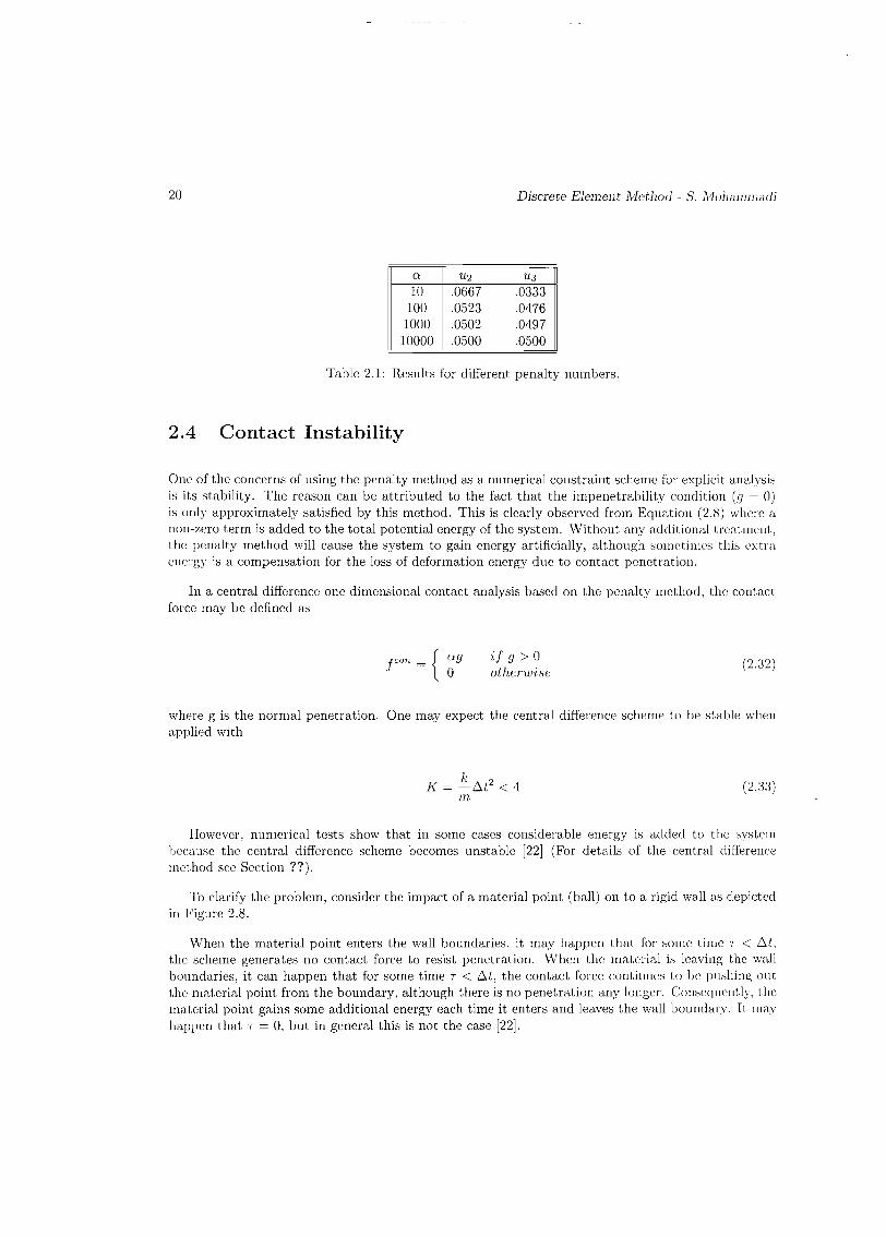
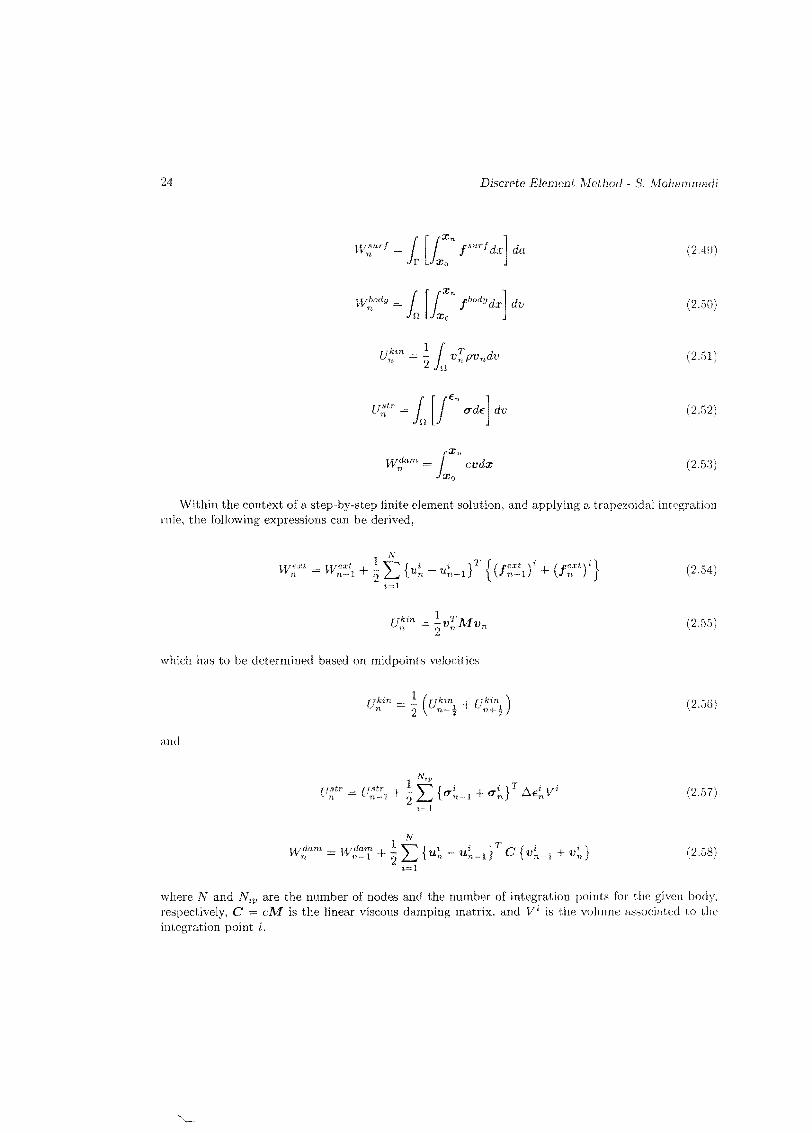


![Ai-ThinkerCopyright(c)2017 · 2019. 7. 9. · X"Ñ 9 + FJ. F65 /j,´ õ å ; ) \ { ¼,´ µ éF >| i,´ s Y Ä \ { ¼ õ j ¯+X 7 , È$! c 2 ¹ 0 ° 9L ( m Ë X \ { ¼ ] Ë ö. ,´](https://img.pdfslide.us/doc/110x75/60d3fde7d155612f55341047/ai-thinkercopyrightc2017-2019-7-9-x-9-fj-f65-j-.jpg)


![fj k - sssc.uk.gov.in · T - ] 101) ge - 3 27. ) t ) e ) m ) e 27. & ) j ) a 28. ) h ) t ) t ) y 28. \ ) k ) e ) Z) k 29. ) ve](https://img.pdfslide.us/doc/110x75/5bb9cb1109d3f27c3d8cb5bd/fj-k-ssscukgovin-t-101-ge-3-27-t-e-m-e-27-j-a-28.jpg)
![RMMWG ULG lL Y[O dW JLGERMT RM )95% fj dd o^ c] sapps.startribune.com/eedition_ipad/pdfs/2017/02/08... · RMMWG ULG lL Y[O dW JLGERMT RM )95% fj dd o^ c] s ... [n )](https://img.pdfslide.us/doc/110x75/5e51171d36ee5e0b3a562ab6/rmmwg-ulg-ll-yo-dw-jlgermt-rm-95-fj-dd-o-c-sapps-rmmwg-ulg-ll-yo-dw-jlgermt.jpg)