In this approach to 3D seismic survey design, I will say lit-tle about bin size and fold because these two concepts candetract from more important issues in 3D survey design.Focusing on fold and bin size for their own sake can ofteninhibit thinking more broadly about the concepts of imag-ing and signal versus noise qualities of a seismic program.

The technical emphasis will be on trace density and sta-tistical diversity. Since we live in a very real world whereany type of “ideal” model is likely to be distorted duringimplementation, we are also concerned with robustnessunder perturbation. I hope that all companies in the seis-mic data acquisition business will also want to minimizeenvironmental impact and I know that all will be aware ofsurvey costs. Since these last two considerations will influ-ence a survey’s source and receiver layout, they must weighinto our choice of design type and parameters.

This article, the first part of a two-part tutorial, willreview methods of estimating signal and understandingnoise in a given project area, discuss the concepts of tracedensity and statistical diversity, address concepts in prestackmigration, and review the concept of bin size. One exam-ple of the misleading nature of the concept of fold will beshown to underscore the importance of diversity. The sec-ond part of this tutorial—to be published in December’sTLE—begins with a brief discussion of the merits of vari-ous model types, which will lead to a discussion of robust-ness during implementation. I will suggest a data simulationmethod to evaluate the characteristics of a design.

Estimating signal. One of the first concerns when design-ing a survey is to identify the nature of the key targets tobe imaged. In particular, we are generally interested in theuseable offsets, wavefield complexity (shortest apparentwavelengths required), and relative signal strength. Theseshould be considered for all significant reflections used inthe interpretation of the target prospect. We should alsoconsider targets that may be of importance to other usersof the data both now and in the future.

Often, we use simple calculations to estimate these fac-tors. Such calculations should be used as guidelines only.Figure 1 shows one example of the results of such calcula-tions. (The equations used are summarized in the appen-dix.) By using estimates of refraction and direct wavevelocities, two-way traveltimes and stacking velocities fora series of reflectors, we can estimate the maximum useableoffset beyond which first break mutes and/or stretch muteslimit the use of far-offset data.

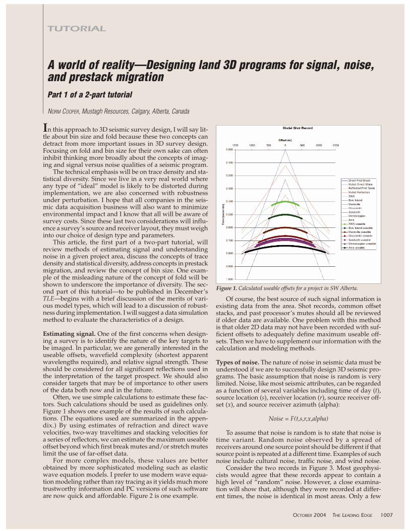
For more complex models, these values are betterobtained by more sophisticated modeling such as elasticwave equation models. I prefer to use modern wave equa-tion modeling rather than ray tracing as it yields much moretrustworthy information and PC versions of such softwareare now quick and affordable. Figure 2 is one example.

Of course, the best source of such signal information isexisting data from the area. Shot records, common offsetstacks, and past processor’s mutes should all be reviewedif older data are available. One problem with this methodis that older 2D data may not have been recorded with suf-ficient offsets to adequately define maximum useable off-sets. Then we have to supplement our information with thecalculation and modeling methods.

Types of noise. The nature of noise in seismic data must beunderstood if we are to successfully design 3D seismic pro-grams. The basic assumption that noise is random is verylimited. Noise, like most seismic attributes, can be regardedas a function of several variables including time of day (t),source location (s), receiver location (r), source receiver off-set (x), and source receiver azimuth (alpha):

Noise = F(t,s,r,x,alpha)

To assume that noise is random is to state that noise istime variant. Random noise observed by a spread ofreceivers around one source point should be different if thatsource point is repeated at a different time. Examples of suchnoise include cultural noise, traffic noise, and wind noise.

Consider the two records in Figure 3. Most geophysi-cists would agree that these records appear to contain ahigh level of “random” noise. However, a close examina-tion will show that, although they were recorded at differ-ent times, the noise is identical in most areas. Only a few

OCTOBER 2004 THE LEADING EDGE 1007

A world of reality—Designing land 3D programs for signal, noise,and prestack migrationPart 1 of a 2-part tutorial

NORM COOPER, Mustagh Resources, Calgary, Alberta, Canada

TUTORIAL

Figure 1. Calculated useable offsets for a project in SW Alberta.

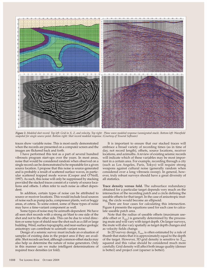
traces show variable noise. This is most easily demonstratedwhen the records are presented on a computer screen and theimages are flickered back and forth.

I have performed this test as a part of several hundredvibroseis program start-ups over the years. In most areas,noise that would be considered random when observed on asingle record can be demonstrated to be repeatable for a givensource location. I propose that this noise is source-generatedand is probably a result of scattered surface waves, in partic-ular scattered trapped mode waves (Cooper and O’Neill,1997). As such, this noise will only be suppressed by stackingprovided the stacked traces consist of a variety of source loca-tions and offsets. I often refer to such noise as offset depen-dent.

In addition, certain types of noise can be attributed tosource or receiver locations. This would include local sourcesof noise such as pump jacks, compressor plants, wet or boggyareas, et cetera. To some extent, some of these types of noisemay have a time-variant component as well.

Some types of noise may be azimuth-dependent. We haveall seen shot records with a strong air blast to one side of theshot and not to the other side. This can be due to wind direc-tion or some type of shield near the shot such as a cliff or largebuilding. Wind, surface topography, and near-surface geologicanisotropy can contribute to azimuth variant noise.

Design of a seismic survey must include an evaluation ofsamples of existing data in the project area if they are avail-able. Shot records are best, although common-offset stacks mayalso help us determine the nature of noise generators. Onlyin this manner can we make intelligent determinations ofrequired trace densities (or fold).

It is important to ensure that our stacked traces willembrace a broad variety of recording times (as in time ofday, not record length), offsets, source locations, receiverlocations, and azimuths. Areview of existing seismic recordswill indicate which of these variables may be most impor-tant in a certain area. For example, recording through a city(such as Los Angeles, Paris, Tokyo) will require strongweapons against cultural noise (generally random whenconsidered over a long vibroseis sweep). In general, how-ever, truly robust surveys should have a great diversity ofall statistics.

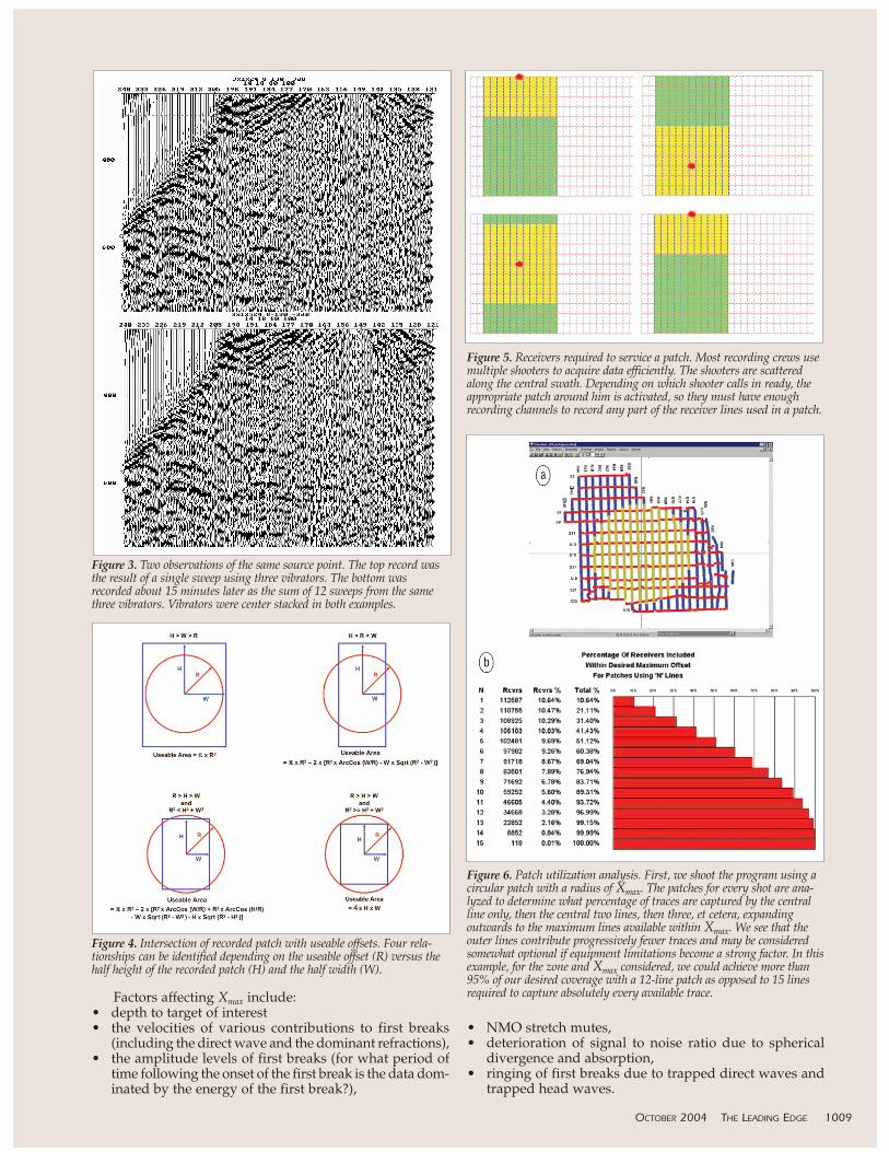
Trace density versus fold. The subsurface redundancyobtained for a particular target depends very much on theintersection of the recording patch and a circle defining theuseable offsets for that target. In the case of anisotropic mut-ing, the circle would become an ellipsoid.

There are four cases for calculating this intersection.Figure 4 presents the equations used for each case to calcu-late useable patch area.

Note that the radius of useable offsets (maximum use-able offset or Xmax) is generally determined by the process-ing mute and will vary with target depth. On larger surveys,the mute will also vary spatially as target depth changes andas velocity fields change.

In 2D survey design, Xmax is often estimated by a rule ofthumb that states that it is approximately equal to the depthof the target. However, 3D grid density is sensitive to Xmaxsquared and this value should be considered much morecarefully. Grid density will affect both image quality (denseris better) and project cost (sparser is better).

1008 THE LEADING EDGE OCTOBER 2004

Figure 2. Modeled shot record. Top left: Grid in X, Z, and velocity. Top right: Plane wave modeled response (unmigrated stack). Bottom left: Wavefieldsnapshot for single source point. Bottom right: Shot record modeled response. (Courtesy of Tesseral Software)

Factors affecting Xmax include:• depth to target of interest• the velocities of various contributions to first breaks

(including the direct wave and the dominant refractions), • the amplitude levels of first breaks (for what period of

time following the onset of the first break is the data dom-inated by the energy of the first break?),

• NMO stretch mutes,• deterioration of signal to noise ratio due to spherical

divergence and absorption,• ringing of first breaks due to trapped direct waves and

trapped head waves.

OCTOBER 2004 THE LEADING EDGE 1009

Figure 3. Two observations of the same source point. The top record wasthe result of a single sweep using three vibrators. The bottom wasrecorded about 15 minutes later as the sum of 12 sweeps from the samethree vibrators. Vibrators were center stacked in both examples.

Figure 4. Intersection of recorded patch with useable offsets. Four rela-tionships can be identified depending on the useable offset (R) versus thehalf height of the recorded patch (H) and the half width (W).

Figure 5. Receivers required to service a patch. Most recording crews usemultiple shooters to acquire data efficiently. The shooters are scatteredalong the central swath. Depending on which shooter calls in ready, theappropriate patch around him is activated, so they must have enoughrecording channels to record any part of the receiver lines used in a patch.

Figure 6. Patch utilization analysis. First, we shoot the program using acircular patch with a radius of Xmax. The patches for every shot are ana-lyzed to determine what percentage of traces are captured by the centralline only, then the central two lines, then three, et cetera, expandingoutwards to the maximum lines available within Xmax. We see that theouter lines contribute progressively fewer traces and may be consideredsomewhat optional if equipment limitations become a strong factor. In thisexample, for the zone and Xmax considered, we could achieve more than95% of our desired coverage with a 12-line patch as opposed to 15 linesrequired to capture absolutely every available trace.

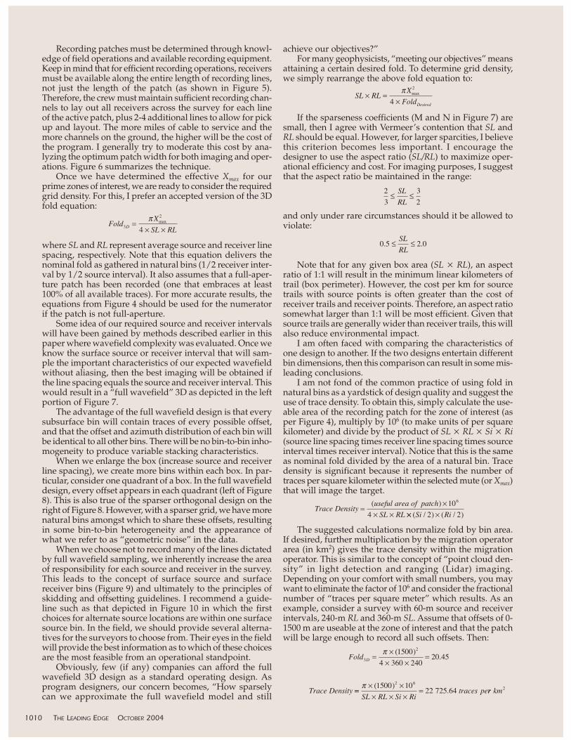
Recording patches must be determined through knowl-edge of field operations and available recording equipment.Keep in mind that for efficient recording operations, receiversmust be available along the entire length of recording lines,not just the length of the patch (as shown in Figure 5).Therefore, the crew must maintain sufficient recording chan-nels to lay out all receivers across the survey for each lineof the active patch, plus 2-4 additional lines to allow for pickup and layout. The more miles of cable to service and themore channels on the ground, the higher will be the cost ofthe program. I generally try to moderate this cost by ana-lyzing the optimum patch width for both imaging and oper-ations. Figure 6 summarizes the technique.

Once we have determined the effective Xmax for ourprime zones of interest, we are ready to consider the requiredgrid density. For this, I prefer an accepted version of the 3Dfold equation:

where SL and RL represent average source and receiver linespacing, respectively. Note that this equation delivers thenominal fold as gathered in natural bins (1/2 receiver inter-val by 1/2 source interval). It also assumes that a full-aper-ture patch has been recorded (one that embraces at least100% of all available traces). For more accurate results, theequations from Figure 4 should be used for the numeratorif the patch is not full-aperture.

Some idea of our required source and receiver intervalswill have been gained by methods described earlier in thispaper where wavefield complexity was evaluated. Once weknow the surface source or receiver interval that will sam-ple the important characteristics of our expected wavefieldwithout aliasing, then the best imaging will be obtained ifthe line spacing equals the source and receiver interval. Thiswould result in a “full wavefield” 3D as depicted in the leftportion of Figure 7.

The advantage of the full wavefield design is that everysubsurface bin will contain traces of every possible offset,and that the offset and azimuth distribution of each bin willbe identical to all other bins. There will be no bin-to-bin inho-mogeneity to produce variable stacking characteristics.

When we enlarge the box (increase source and receiverline spacing), we create more bins within each box. In par-ticular, consider one quadrant of a box. In the full wavefielddesign, every offset appears in each quadrant (left of Figure8). This is also true of the sparser orthogonal design on theright of Figure 8. However, with a sparser grid, we have morenatural bins amongst which to share these offsets, resultingin some bin-to-bin heterogeneity and the appearance ofwhat we refer to as “geometric noise” in the data.

When we choose not to record many of the lines dictatedby full wavefield sampling, we inherently increase the areaof responsibility for each source and receiver in the survey.This leads to the concept of surface source and surfacereceiver bins (Figure 9) and ultimately to the principles ofskidding and offsetting guidelines. I recommend a guide-line such as that depicted in Figure 10 in which the firstchoices for alternate source locations are within one surfacesource bin. In the field, we should provide several alterna-tives for the surveyors to choose from. Their eyes in the fieldwill provide the best information as to which of these choicesare the most feasible from an operational standpoint.

Obviously, few (if any) companies can afford the fullwavefield 3D design as a standard operating design. Asprogram designers, our concern becomes, “How sparselycan we approximate the full wavefield model and still

achieve our objectives?”For many geophysicists, “meeting our objectives” means

attaining a certain desired fold. To determine grid density,we simply rearrange the above fold equation to:

If the sparseness coefficients (M and N in Figure 7) aresmall, then I agree with Vermeer’s contention that SL andRL should be equal. However, for larger sparcities, I believethis criterion becomes less important. I encourage thedesigner to use the aspect ratio (SL/RL) to maximize oper-ational efficiency and cost. For imaging purposes, I suggestthat the aspect ratio be maintained in the range:

and only under rare circumstances should it be allowed toviolate:

Note that for any given box area (SL � RL), an aspectratio of 1:1 will result in the minimum linear kilometers oftrail (box perimeter). However, the cost per km for sourcetrails with source points is often greater than the cost ofreceiver trails and receiver points. Therefore, an aspect ratiosomewhat larger than 1:1 will be most efficient. Given thatsource trails are generally wider than receiver trails, this willalso reduce environmental impact.

I am often faced with comparing the characteristics ofone design to another. If the two designs entertain differentbin dimensions, then this comparison can result in some mis-leading conclusions.

I am not fond of the common practice of using fold innatural bins as a yardstick of design quality and suggest theuse of trace density. To obtain this, simply calculate the use-able area of the recording patch for the zone of interest (asper Figure 4), multiply by 106 (to make units of per squarekilometer) and divide by the product of SL � RL � Si � Ri(source line spacing times receiver line spacing times sourceinterval times receiver interval). Notice that this is the sameas nominal fold divided by the area of a natural bin. Tracedensity is significant because it represents the number oftraces per square kilometer within the selected mute (or Xmax)that will image the target.

The suggested calculations normalize fold by bin area.If desired, further multiplication by the migration operatorarea (in km2) gives the trace density within the migrationoperator. This is similar to the concept of “point cloud den-sity” in light detection and ranging (Lidar) imaging.Depending on your comfort with small numbers, you maywant to eliminate the factor of 106 and consider the fractionalnumber of “traces per square meter” which results. As anexample, consider a survey with 60-m source and receiverintervals, 240-m RL and 360-m SL. Assume that offsets of 0-1500 m are useable at the zone of interest and that the patchwill be large enough to record all such offsets. Then:

1010 THE LEADING EDGE OCTOBER 2004

or 0.0227 traces per m2

or one trace per 44 m2

or one trace per 6.6 by 6.6 m

Provided that the survey statistics (including midpointscatter) are sufficiently diverse, then the last number rep-resents the potential spatial resolution of a broadbandprestack migration. Of course, limits in our recorded band-width usually prevent us from attaining such a resolution.

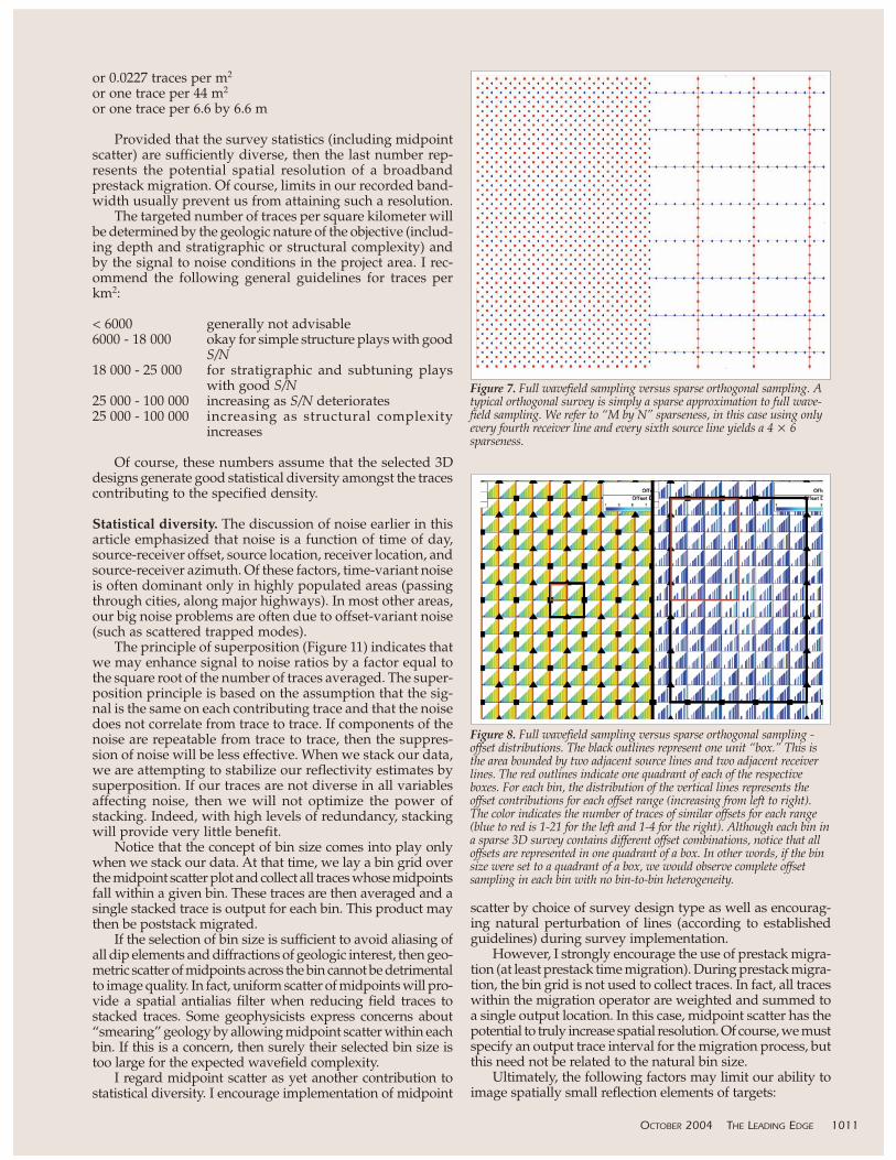
The targeted number of traces per square kilometer willbe determined by the geologic nature of the objective (includ-ing depth and stratigraphic or structural complexity) andby the signal to noise conditions in the project area. I rec-ommend the following general guidelines for traces perkm2:

< 6000 generally not advisable6000 - 18 000 okay for simple structure plays with good

S/N18 000 - 25 000 for stratigraphic and subtuning plays

with good S/N25 000 - 100 000 increasing as S/N deteriorates25 000 - 100 000 increasing as structural complexity

increases

Of course, these numbers assume that the selected 3Ddesigns generate good statistical diversity amongst the tracescontributing to the specified density.

Statistical diversity. The discussion of noise earlier in thisarticle emphasized that noise is a function of time of day,source-receiver offset, source location, receiver location, andsource-receiver azimuth. Of these factors, time-variant noiseis often dominant only in highly populated areas (passingthrough cities, along major highways). In most other areas,our big noise problems are often due to offset-variant noise(such as scattered trapped modes).

The principle of superposition (Figure 11) indicates thatwe may enhance signal to noise ratios by a factor equal tothe square root of the number of traces averaged. The super-position principle is based on the assumption that the sig-nal is the same on each contributing trace and that the noisedoes not correlate from trace to trace. If components of thenoise are repeatable from trace to trace, then the suppres-sion of noise will be less effective. When we stack our data,we are attempting to stabilize our reflectivity estimates bysuperposition. If our traces are not diverse in all variablesaffecting noise, then we will not optimize the power ofstacking. Indeed, with high levels of redundancy, stackingwill provide very little benefit.

Notice that the concept of bin size comes into play onlywhen we stack our data. At that time, we lay a bin grid overthe midpoint scatter plot and collect all traces whose midpointsfall within a given bin. These traces are then averaged and asingle stacked trace is output for each bin. This product maythen be poststack migrated.

If the selection of bin size is sufficient to avoid aliasing ofall dip elements and diffractions of geologic interest, then geo-metric scatter of midpoints across the bin cannot be detrimentalto image quality. In fact, uniform scatter of midpoints will pro-vide a spatial antialias filter when reducing field traces tostacked traces. Some geophysicists express concerns about“smearing” geology by allowing midpoint scatter within eachbin. If this is a concern, then surely their selected bin size istoo large for the expected wavefield complexity.

I regard midpoint scatter as yet another contribution tostatistical diversity. I encourage implementation of midpoint

scatter by choice of survey design type as well as encourag-ing natural perturbation of lines (according to establishedguidelines) during survey implementation.

However, I strongly encourage the use of prestack migra-tion (at least prestack time migration). During prestack migra-tion, the bin grid is not used to collect traces. In fact, all traceswithin the migration operator are weighted and summed toa single output location. In this case, midpoint scatter has thepotential to truly increase spatial resolution. Of course, we mustspecify an output trace interval for the migration process, butthis need not be related to the natural bin size.

Ultimately, the following factors may limit our ability toimage spatially small reflection elements of targets:

OCTOBER 2004 THE LEADING EDGE 1011

Figure 7. Full wavefield sampling versus sparse orthogonal sampling. Atypical orthogonal survey is simply a sparse approximation to full wave-field sampling. We refer to “M by N” sparseness, in this case using onlyevery fourth receiver line and every sixth source line yields a 4 � 6sparseness.

Figure 8. Full wavefield sampling versus sparse orthogonal sampling -offset distributions. The black outlines represent one unit “box.” This isthe area bounded by two adjacent source lines and two adjacent receiverlines. The red outlines indicate one quadrant of each of the respectiveboxes. For each bin, the distribution of the vertical lines represents theoffset contributions for each offset range (increasing from left to right).The color indicates the number of traces of similar offsets for each range(blue to red is 1-21 for the left and 1-4 for the right). Although each bin ina sparse 3D survey contains different offset combinations, notice that alloffsets are represented in one quadrant of a box. In other words, if the binsize were set to a quadrant of a box, we would observe complete offsetsampling in each bin with no bin-to-bin heterogeneity.

• Geologic complexity. Structural dips or diffractions fromlateral velocity changes must exist. If the geology does notcontain lateral velocity or density changes then, of course,we will have nothing to resolve.

• Recoverable bandwidth. The final processed bandwidthat the target zone will not only determine the limit of ver-tical resolution (often stated as a quarter wavelength) butwill also form one limit on spatial resolution (sometimesstated as a half wavelength:

• Output trace spacing after migration (as per Nyquist).

Our job is to ensure that the output trace spacing does notimpose more restrictive limits than those imposed by the firsttwo factors. It would be wasteful of processing time and pro-cessing budget to output more traces than necessary to meetthe limits of the first two factors. I recommend testing outputbin size on a small data cube. The results of one such test arepresented in Figure 12.

Note that if midpoints are tightly focused at natural bincenters, then there is no diversity in the input spatial grid andresolution below that of the natural bin size should not beexpected. On the other hand, with maximum midpoint scat-ter, resolution is potentially achievable to the individual tracearea (6.6 � 6.6 m in our previous trace density example). Ofcourse, midpoint scatter alone cannot ensure spatial resolu-tion without sufficient bandwidth and geologic complexity.

One last word on statistical diversity: While offset andazimuth distribution along with source and receiver locationsare obvious, statistics that require diversity within each bingather, it has been demonstrated that midpoint scatter alsocontributes to diverse sampling. On a more subtle level, boxaspect ratio is also a contributor to statistical diversity in the

1012 THE LEADING EDGE OCTOBER 2004

Figure 9. Surface bins for sources (left) and receivers (right). The area ofresponsibility for each source and receiver is increased when we choose asparse orthogonal design. SL and RL refer to source and receiver linespacing, respectively; si and ri refer to source and receiver intervals alongeach line.

Figure 10. Skid and offset guidelines. A grid of “surface bins” (each binbeing one source interval by one receiver interval in size) is centered on asource point that needs to be relocated. The grid is oriented parallel toreceiver lines. The number in each cell of this “bingo card” represents theorder of preference for a source location. The most preferred locations(numbers 1-5) are defined within the surface source bin corresponding tothe source being moved (indicated by the green outline). Other choicesshould be considered only if choices within the green rectangle are notfeasible.

Figure 11. Principle ofsuperposition. AveragingN traces produces a N1/2

improvement in signal tonoise ratio.

Figure 12. Testing PSTM output trace interval. This is an example froma shallow steam flood project. Each panel is only 50 ms of data. The toppanel was prestack time migrated to a 12-m bin (natural bin size), themiddle panel to an 8-m bin and the bottom panel to a 4-m bin.Frequencies up to 140 Hz were included and the average velocity to thetarget is 2000 m/s. This would lead us to expect potential spatial resolu-tion of about 7.1 m. Note that migration to 8-m bins provides a steeperimage of the front of the steam chamber compared to the 12-m bins.Reducing output trace spacing from 8 to 4 m delivers more traces butdoes not significantly sharpen the image.

case of sparse surveys (Cooper and Herrera, 2002). Providedthe sparseness indices M and N are not very small, some sta-tistical distributions benefit from a moderate box asymmetry.This supports the earlier recommendation to consider someasymmetry in order to optimize survey costs and operations.

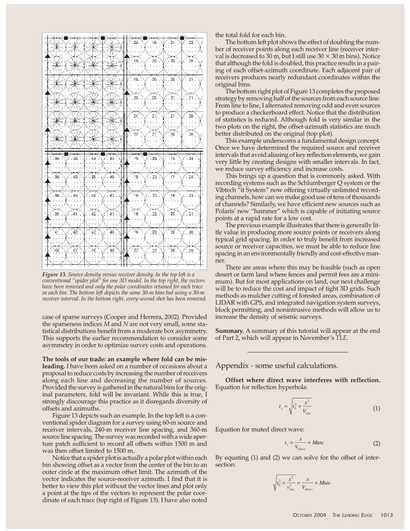
The tools of our trade: an example where fold can be mis-leading. I have been asked on a number of occasions about aproposal to reduce costs by increasing the number of receiversalong each line and decreasing the number of sources.Provided the survey is gathered in the natural bins for the orig-inal parameters, fold will be invariant. While this is true, Istrongly discourage this practice as it disregards diversity ofoffsets and azimuths.

Figure 13 depicts such an example. In the top left is a con-ventional spider diagram for a survey using 60-m source andreceiver intervals, 240-m receiver line spacing, and 360-msource line spacing. The survey was recorded with a wide aper-ture patch sufficient to record all offsets within 1500 m andwas then offset limited to 1500 m.

Notice that a spider plot is actually a polar plot within eachbin showing offset as a vector from the center of the bin to anouter circle at the maximum offset limit. The azimuth of thevector indicates the source-receiver azimuth. I find that it isbetter to view this plot without the vector lines and plot onlya point at the tips of the vectors to represent the polar coor-dinate of each trace (top right of Figure 13). I have also noted

the total fold for each bin.The bottom left plot shows the effect of doubling the num-

ber of receiver points along each receiver line (receiver inter-val is decreased to 30 m, but I still use 30 � 30 m bins). Noticethat although the fold is doubled, this practice results in a pair-ing of each offset-azimuth coordinate. Each adjacent pair ofreceivers produces nearly redundant coordinates within theoriginal bins.

The bottom right plot of Figure 13 completes the proposedstrategy by removing half of the sources from each source line.From line to line, I alternated removing odd and even sourcesto produce a checkerboard effect. Notice that the distributionof statistics is reduced. Although fold is very similar in thetwo plots on the right, the offset-azimuth statistics are muchbetter distributed on the original (top plot).

This example underscores a fundamental design concept.Once we have determined the required source and receiverintervals that avoid aliasing of key reflection elements, we gainvery little by creating designs with smaller intervals. In fact,we reduce survey efficiency and increase costs.

This brings up a question that is commonly asked. Withrecording systems such as the Schlumberger Q system or theVibtech “it System” now offering virtually unlimited record-ing channels, how can we make good use of tens of thousandsof channels? Similarly, we have efficient new sources such asPolaris’ new “hammer” which is capable of initiating sourcepoints at a rapid rate for a low cost.

The previous example illustrates that there is generally lit-tle value in producing more source points or receivers alongtypical grid spacing. In order to truly benefit from increasedsource or receiver capacities, we must be able to reduce linespacing in an environmentally friendly and cost-effective man-ner.

There are areas where this may be feasible (such as opendesert or farm land where fences and permit fees are a mini-mum). But for most applications on land, our next challengewill be to reduce the cost and impact of tight 3D grids. Suchmethods as mulcher cutting of forested areas, combination ofLIDAR with GPS, and integrated navigation system surveys,block permitting, and nonintrusive methods will allow us toincrease the density of seismic surveys.

Summary. A summary of this tutorial will appear at the endof Part 2, which will appear in November’s TLE.

Appendix - some useful calculations.

Offset where direct wave interferes with reflection.Equation for reflection hyperbola:

(1)

Equation for muted direct wave:

(2)

By equating (1) and (2) we can solve for the offset of inter-section:

OCTOBER 2004 THE LEADING EDGE 1013

Figure 13. Source density versus receiver density. In the top left is aconventional “spider plot” for one 3D model. In the top right, the vectorshave been removed and only the polar coordinates retained for each tracein each bin. The bottom left depicts the same 30-m bins but using a 30-mreceiver interval. In the bottom right, every second shot has been removed.

Solving for x yields:

where:

The same derivation applies to interference with a refractedwave with the following modifications:

• substitute Vrefractor for Vdirect• the mute should include the intercept time for the refrac-

tion

Offset of sufficient NMO for velocity analysis. Equation forreflection hyperbola:

At what offset does tx - t0 = P, where P is 1.5 times the domi-nant period of the data?

Solving for x yields:

The same derivation applies to the calculation of sufficientNMO for multiple cancellation with the following modifica-tions:

• substitute Vmultiple for Vrms• P should be 3.0 times the dominant period of the data

Offset where NMO stretch limit first occurs. Normal move-out corrections are applied to data in the course of process-ing. Since this is a dynamic process, the correction applied atone point in time is not the same as the correction applied ata different point in time (except at the zero-offset trace). Thisresults in a stretching of data that distorts wavelet character-istics. Most NMO programs mute data that is stretched morethan a specified percentage. This percentage can be specifiedas the difference in moveout corrections for two points dividedby the original separation of those two points. A formula forNMO stretch at a point is derived by taking the limit of thisratio as the time separation of the two events approaches zero.Expressed as a percent this is of the form:

where:

and:

Or:

which we recognize as:

Taking the derivatives of F(t0) and G(t0) and solving for xyields:

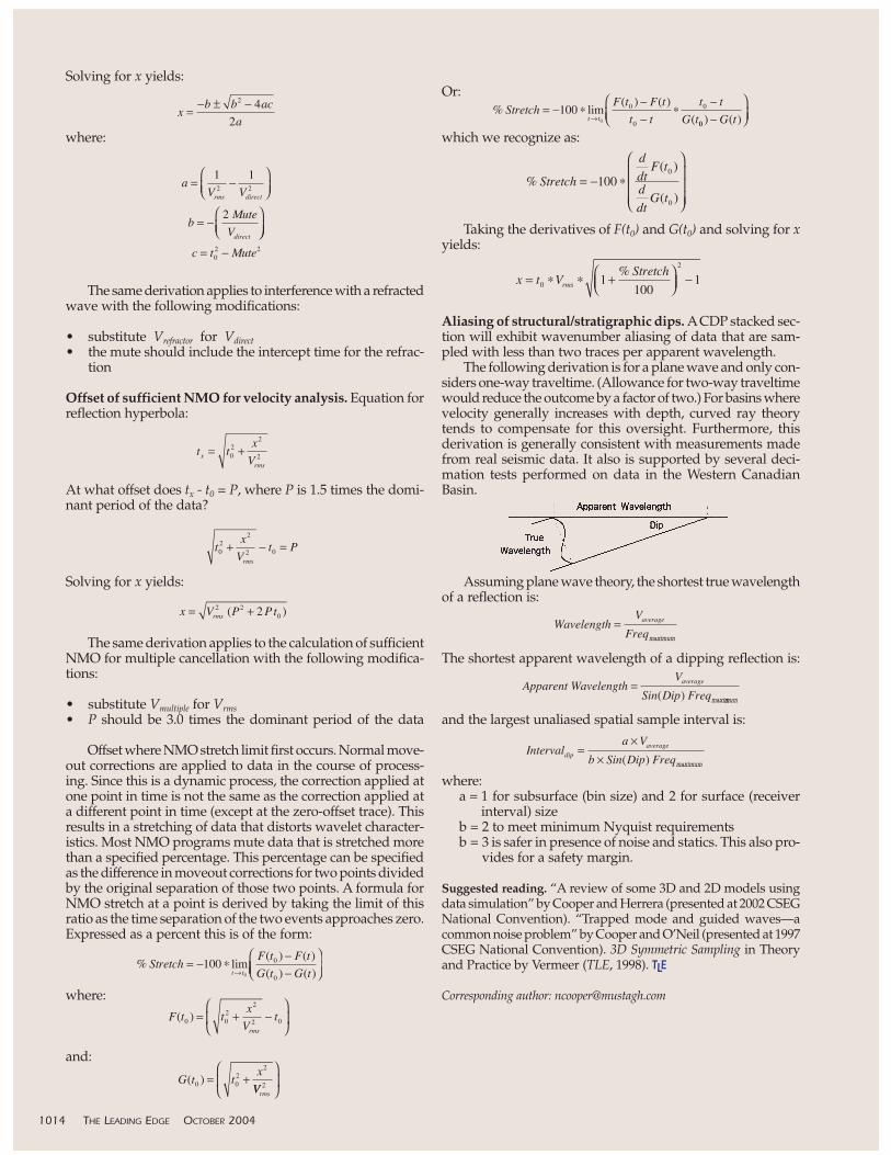
Aliasing of structural/stratigraphic dips. ACDP stacked sec-tion will exhibit wavenumber aliasing of data that are sam-pled with less than two traces per apparent wavelength.

The following derivation is for a plane wave and only con-siders one-way traveltime. (Allowance for two-way traveltimewould reduce the outcome by a factor of two.) For basins wherevelocity generally increases with depth, curved ray theorytends to compensate for this oversight. Furthermore, thisderivation is generally consistent with measurements madefrom real seismic data. It also is supported by several deci-mation tests performed on data in the Western CanadianBasin.

Assuming plane wave theory, the shortest true wavelengthof a reflection is:

The shortest apparent wavelength of a dipping reflection is:

and the largest unaliased spatial sample interval is:

where:a = 1 for subsurface (bin size) and 2 for surface (receiver

interval) sizeb = 2 to meet minimum Nyquist requirementsb = 3 is safer in presence of noise and statics. This also pro-

vides for a safety margin.

Suggested reading. “A review of some 3D and 2D models usingdata simulation” by Cooper and Herrera (presented at 2002 CSEGNational Convention). “Trapped mode and guided waves—acommon noise problem” by Cooper and O’Neil (presented at 1997CSEG National Convention). 3D Symmetric Sampling in Theoryand Practice by Vermeer (TLE, 1998). TLE

Corresponding author: ncooper@mustagh.com

1014 THE LEADING EDGE OCTOBER 2004