A Weighted Voting Framework for Classifiers Ensembles

Knowl Inf SystDOI 10.1007/s10115-012-0586-6

REGULAR PAPER

A weighted voting framework for classifiers ensembles

Ludmila I. Kuncheva · Juan J. Rodríguez

Received: 15 August 2011 / Revised: 27 July 2012 / Accepted: 24 November 2012© Springer-Verlag London 2012

Abstract We propose a probabilistic framework for classifier combination, which gives rig-orous optimality conditions (minimum classification error) for four combination methods:majority vote, weighted majority vote, recall combiner and the naive Bayes combiner. Theframework is based on two assumptions: class-conditional independence of the classifieroutputs and an assumption about the individual accuracies. The four combiners are derivedsubsequently from one another, by progressively relaxing and then eliminating the secondassumption. In parallel, the number of the trainable parameters increases from one combinerto the next. Simulation studies reveal that if the parameter estimates are accurate and thefirst assumption is satisfied, the order of preference of the combiners is: naive Bayes, recall,weighted majority and majority. By inducing label noise, we expose a caveat coming fromthe stability-plasticity dilemma. Experimental results with 73 benchmark data sets revealthat there is no definitive best combiner among the four candidates, giving a slight prefer-ence to naive Bayes. This combiner was better for problems with a large number of fairlybalanced classes while weighted majority vote was better for problems with a small numberof unbalanced classes.

Keywords Classifier ensembles · Combination rules · Weighted majority vote · Recall ·Naive Bayes

1 Introduction

Classifier ensembles are justly receiving increasing attention and accolade and generatinga wealth of research [1,22,23,25,29]. Theoretical and empirical studies have demonstrated

L. I. Kuncheva (B)School of Computer Science, Bangor University, Dean Street, Bangor Gwynedd LL57 1UT, UKe-mail: [email protected]

J. J. RodríguezDepartamento de Ingeniería Civil, Universidad de Burgos, Burgos, Spaine-mail: [email protected]

123

L. I. Kuncheva, J. J. Rodríguez

that an ensemble of classifiers is typically more accurate than a single classifier. Researchon classifier ensembles permeate many strands machine learning including streaming data[9,24], concept drift and incremental learning [5].

One of the basic design questions is what combination rule (combiner) to use. Majority voteand weighted majority vote are the most widespread choices when the individual classifiersgive label outputs [15]. One of the great assets of the majority vote combiner is that itdoes not require any parameter tuning once the individual classifiers have been trained. Ithas been about a decade since Bob Duin posed the question “To Train or not to Train?”[2], and exposed potential caveats in tuning the parameters of the combiner. Choosing theright combiner for the classification problem is not discussed very often, and preferencesare given to uncomplicated combiners such as majority vote, average and their weightedversions. Theoretical analyses [7,12,13,16,17,19,28] and experimental comparisons [3,8,14,27,30,31] of classifier combiners do not offer a definitive answer or a recipe to guide thischoice.

Here, we propose a common probabilistic framework for the following four combinationmethods: majority vote1 (MV), weighted majority vote (WMV), recall (REC) and naive Bayes(NB). Each combiner is obtained from the previous one when a certain assumption is relaxedor dropped. The price to pay is that each combiner needs more tunable parameters than theprevious one. We compare the four combiners on simulated data and on 73 benchmark datasets with a view to propose a strategy to choose among the four combiners.

The rest of the paper is organised as follows. Section 2 introduces the proposed frameworkand details the four combiners as special cases thereof. Section 3 contains a simulation studyand Sect. 4, the experimental protocol and results.

2 A weighted voting framework for classifier ensembles

2.1 Probabilistic set-up

Consider a set of classes � = {ω1, . . . , ωc} and a classifier ensemble of L classifiers. Denoteby si the class label proposed by classifier i (si ∈ �). We are interested in the probability

P(ωk is the true class | s1, s2, . . . , sL), k = 1, . . . , c,

denoted for short P(ωk |s), where s = [s1, s2, . . . , sL ]T is a label vector. Assume that theclassifiers give their decisions independently conditioned upon the class label,2 which leadsto the following decomposition

P(ωk |s) = P(ωk)

P(s)

L∏

i=1

P(si |ωk) (1)

1 This should be called rather the plurality vote because the assigned label is the most voted one, in spite ofthe fact that majority of more than 50 % may not be reached.2 Conditional independence means that

P(s1, s2, . . . , sL |ωk ) = P(s1|ωk )P(s2|ωk ) . . . P(sL |ωk ).

However, this assumption precludes unconditional independence, that is,

P(s1, s2, . . . , sL ) �= P(s1)P(s2) . . . P(sL ).

123


Split the product into two parts depending on which classifiers suggested ωk . Denote by I k+the set of indices of classifiers which suggested ωk , and by I k− the set of indices of classifierswhich suggested another class label. The probability of interest becomes

P(ωk |s) = P(ωk)

P(s)×

∏

i∈I k+

P(si = ωk |ωk) ×∏

i∈I k−

P(si = ωk |ωk) (2)

All four combiners described next rely upon the same conditional independence assump-tion. They differ on the following assumption about the individual accuracies of the classifiers.If the assumption is met, the respective combiner is optimal in the sense that it guaranteesthe minimum Bayes error.

– Equal individual accuracies. When P(si = ωk |ωk) = p and P(si = ω j |ωk) =1−pc−1 , for any i = 1, . . . , L , k, j = 1, . . . , c j �= k, then majority vote is the optimalcombination rule. Note that for the optimality to hold, not only the accuracies shouldbe equal but also the “leftover” should be uniformly distributed across the remainingclasses.

– Different individual accuracies. When P(si = ωk |ωk) = pi and P(si = ω j |ωk) =1−pic−1 , for any k, j = 1, . . . , c j �= k, then the weighted majority vote is the optimal

combiner with weights as derived in Sect. 2.3.– Different individual class-specific recalls. When P(si = ωk |ωk) = pik and P(si =

ω j |ωk) = 1−pikc−1 , for any k, j = 1, . . . , c j �= k, then the recall combiner is the optimal

combiner. The details are derived in Sect. 2.4.– Different confusion matrices. When P(si = ω j |ωk) = pi jk , then the Naive Bayes

combiner is the optimal combiner.

The optimality of the combiner, however, is asymptotic, and holds for sample sizeapproaching infinity. For finite sample sizes, the accuracy of the estimates of the parametersmay be the primary concern. A combiner with fewer tunable parameters may be prefer-able even though its optimality assumption does not hold. This issue will appear later as animportant lesson from the experimental study.

2.2 Majority vote (MV)

To give a correct label, “proper” majority vote requires that more than 50 % of the votersgive the correct label. If all classifiers have the same accuracy P(si = ωk |ωk) = p for anyi = 1, . . . , L and k = 1, . . . , c, then the majority vote will be correct if Lmaj = � L

2 � + 1 ormore votes are correct. Then,

Pproper MV =L∑

i=Lmaj

(L

i

)pi (1 − p)(L−i) (3)

The Condorcet Jury Theorem, dated back in 1785 (cited after [26]), states that

1. If p > 0.5, then Pproper MV is monotonically increasing and tends to 1 as L → ∞.2. If p < 0.5, then Pproper MV is monotonically decreasing and tends to 0 as L → ∞.3. If p = 0.5, then Pproper MV = 0.5 for any L .

Lam and Suen [18] analyse the cases of odd and even L and the effect on the ensembleaccuracy of adding or removing classifiers. Shapley and Grofman [26] note that the resultis valid even for unequal individual accuracies, provided their distributions are symmetrical

123


about the mean. Matan [21] gives tight upper and lower bounds of the majority vote accuracyin the case of unequal individual accuracies.

Here, we consider majority vote in the wider sense of the word, as a synonym of pluralityvote. In this case, there is no requirement that more than 50 % of the voters are correct forthe majority to be correct. If there are many classes, a much smaller percentage may suffice.In the absence of further information about the classifiers, assume that all incorrect labels“share” the misclassification probability, that is,

P(si = ω j |ωk) j �=k = (1 − p)

(c − 1). (4)

Substituting in the probabilistic framework defined in (2),

P(ωk |s) = P(ωk)

P(s)×

∏

i∈I k+

p ×∏

i∈I k−

1 − p

c − 1(5)

= P(ωk)

P(s)×

∏

i∈I k+

p ×∏

i∈I k−

1 − p

c − 1×

∏i∈I k+

1−pc−1

∏i∈I k+

1−pc−1

(6)

= P(ωk)

P(s)×

∏

i∈I k+

p(c − 1)

1 − p×

L∏

i=1

1 − p

c − 1(7)

Notice that P(s) and the last product term in (7) do not depend on the class label. Theprior probability, P(ωk), does depend on the class label but not on the votes, so it can bedesignated as the class constant. Rearranging and taking the logarithm,

log(P(ωk |s)) = log

((1 − p)L

P(s)(c − 1)L

)+ log (P(ωk))

+ log

(p(c − 1)

1 − p

)× |I k+|, (8)

where |.| denotes cardinality. Dividing by log(

p(c−1)1−p

)and dropping all terms that do not

depend on the class label or the vote counts, (8) becomes

log(P(ωk |s)) ∝ log

(1 − p

p(c − 1)

)log (P(ωk))

︸︷︷︸class constant ζ(ωk)

+|I k+|. (9)

Note that |I k+| is the number of votes for ωk . Choosing the class label corresponding to thelargest posterior probability is equivalent to choosing the class most voted for, subject to aconstant term. Interestingly, the standard majority vote rule does not include a class constant,and is still one of the most robust and accurate combiners for classifier ensembles. Besides,including the class constant will make MV a trainable combiner, which eliminates one of itsmain assets. Since one of our aims is to give practical recommendations, in the experimentsin this study, we adopted the standard majority vote formulation, whereby the class label isobtained by

ω = arg maxk

|I k+|. (10)

123


2.3 Weighted majority vote (WMV)

The weighted majority vote is among the most intuitive and widely used combiners [11,20].It is the designated combination method derived from minimising a bound on the trainingerror in AdaBoost [4,6]. Freund and Schapire [6] offer a similar probabilistic explanation asan alternative justification for the weights in the two-class version of AdaBoost. Here, we useour framework to derive the multi-class version of the weighted majority vote, and specifythe conditions for its optimality.

The weighted majority vote follows from relaxing the assumption about equal individualaccuracies. Thus, it will be the optimal combiner when the accuracies are equal as well,and the MV combiner is its exact reduced version. Let P(si = ωk |ωk) = pi and P(si =ω j |ωk) = 1−pi

c−1 , for any k, j = 1, . . . , c j �= k. Following the same derivation path as withMV, Eq. (2) becomes

P(ωk |s) = P(ωk)

P(s)×

∏

i∈I k+

pi ×∏

i∈I k−

1 − pi

c − 1(11)

= P(ωk)

P(s)×

∏

i∈I k+

pi (c − 1)

1 − pi×

L∏

i=1

1 − pi

c − 1(12)

= 1

P(s)×

L∏

i=1

1 − pi

c − 1× P(ωk) ×

∏

i∈I k+

pi (c − 1)

1 − pi. (13)

Then,


(∏Li=1(1 − pi )

P(s)(c − 1)L

)+ log (P(ωk))

+∑

i∈|I k+|log

(pi

1 − pi

)+ |I k+| × log(c − 1). (14)

Dropping the first term, which will not influence the class decision, and expressing theclassifier weights as

wi = log

(pi

1 − pi

), 0 < pi < 1,

Equation (14) leads to

log(P(ωk |s)) ∝ log (P(ωk))︸︷︷︸class constant ζ(ωk)

+∑

i∈|I k+|wi + |I k+| × log(c − 1). (15)

If pi = p for all i = 1, . . . , L , Eq. (15) reduces to the majority vote Eq. (8).

2.4 Recall combiner (REC)

The next logical step in relaxing the assumptions is to allow different probabilities of correctclassification depending on the classifier and the class, P(si = ωk |ωk) = pik . This amountsto different individual class-specific recalls. The idea is that each class is considered sepa-rately versus the union of the remaining classes. We assume again that the misclassification

123


probability is shared among the remaining (wrong) classes, that is, P(si = ω j |ωk) = 1−pikc−1 ,

for any k, j = 1, . . . , c, j �= k. Starting again with Eq. (2),

P(ωk |s) = P(ωk)

P(s)×

∏

i∈I k+

pik ×∏

i∈I k−

1 − pik

c − 1(16)

= P(ωk)

P(s)×

∏

i∈I k+

pik(c − 1)

1 − pik×

L∏

i=1

1 − pik

c − 1(17)

This time the last product depends on the class label ωk but not on the decisions in s. Therefore,it will be part of the class constant. Rearranging and taking the logarithm,


(1

P(s)(c − 1)L

)+ log (P(ωk)) +

L∑

i=1

log (1 − pik)

+∑

i∈|I k+|log

(pik

1 − pik

)+ |I k+| × log(c − 1). (18)

Dropping the first term, and denoting the recall weights by

vik = log

(pik

1 − pik

), 0 < pik < 1,

we arrive at

log(P(ωk |s)) ∝ log (P(ωk)) +L∑

i=1

log (1 − pik)

︸︷︷︸class constant ζ(ωk)

+∑

i∈|I k+|vik

+|I k+| × log(c − 1). (19)

If pik = pi for any k = 1, . . . , c, Eq. (19) reduces to the weighted majority vote Eq. (15).To best of our knowledge, the recall combiner has not been used before. It arose from the

logical sequence of relaxing the assumption of equal individual accuracies, falling betweentwo well- known combiners: the weighted majority vote and naive Bayes.

2.5 Naive Bayes combiner (NB)

The Naive Bayes combiner has been acclaimed for its rigorous statistical underpinning androbustness. We can derive this combiner by finally dropping the assumption of equal indi-vidual accuracies, that is, allowing for P(si = ω j |ωk) = pi jk . We can think of pi jk as the( j, k)th entry in a probabilistic confusion matrix for classifier i in the ensemble. In this case,


(1

P(s)

)+ log(P(ωk)) +

L∑

i=1

log (P(si |ωk)) (20)

∝ log (P(ωk))︸︷︷︸class constant ζ(ωk)

+L∑

i=1

log(pi,si ,k). (21)

123


Table 1 Scopes of optimality (denoted by a black square) and the number of tunable parameters of the 4combiners for a problem with c classes and an ensemble of L classifiers

Combiner 1 2 3 4 Number of parameters

Majority vote � – – – none

Weighted majority vote � � – – L + c

Recall � � � – L ∗ (c + 1)

Naive Bayes � � � � L ∗ c2 + c

Column headings: 1 Equal p, 2 Classifier-specific pi , 3 Classifier- and class-specific pi , 4 Full confusionmatrix

2.6 Overview of the four combiners

The progressive relaxation of the assumption means that the combiners have a nested opti-mality scope. The enlargement of the optimality scope is paid by acquiring more tunableparameters. Table 1 shows the optimality scopes and the number of tunable parameters foreach combiner. The additional c parameters are for estimating the prior probabilities for theclasses.

It is tempting to use always Naive Bayes because it has the largest optimality scope. Inpractice, however, the success of a particular combiner will depend partly on the assumptionsand partly on the availability of sufficient data to make reliable estimates of the parameters.Non-optimal but more robust combiners may fare better than the optimal combiner. Thesimulation and the experimental studies described next highlight the importance of this issuewhen choosing a combiner.

Curiously, the well-known and widely used majority vote, weighted majority vote andNaive Bayes combiners typically ignore the class constant (Eqs. (9), (15), and (21), respec-tively). This means that these combination methods will be optimal only if we add to theircurrent set of assumptions the assumption that the classes are equiprobable. The same argu-ment holds for the recall combiner Eq. (19), but this combiner came as a byproduct of theproposed framework and does not enjoy the popularity of the other three combiners.

3 A simulation study

3.1 Protocol

Experiments with simulated classifier outputs were carried out as follows:

– Number of classes c ∈ {2, 3, 4, 5, 10, 20, 50};– Number of classifiers L ∈ {2, 3, 4, 5, 10, 20, 50};– Number of instances (labels) 500;– Number of runs 100.

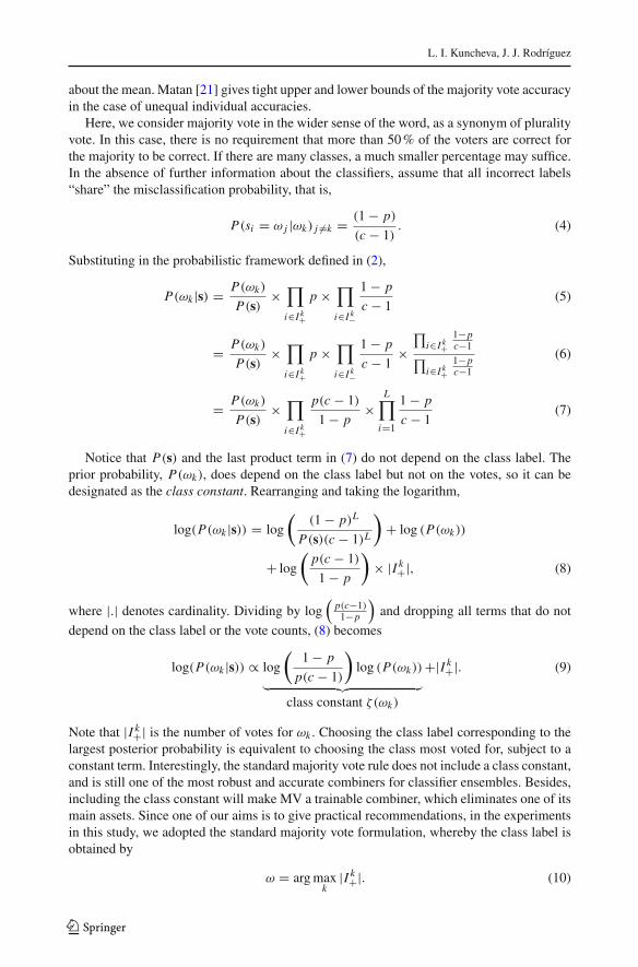
For each run, c classes were generated by labelling the 500 instances according to asymmetric Dirichlet distribution.3 To enforce class-conditional independence, the classifiersin the ensemble were constructed class by class as shown in the Algorithm in Fig. 1. To formthe label set of classifier i and class k, take the labels for class k and replace a percentagebetween 0 and 66.7 % with labels randomly sampled from �. The c sets of labels for each

3 Each set of c random numbers summing up to 1 had the same chance of being generated.

123


Fig. 1 Algorithm for generating ‘true’ class labels and class-conditional independent outputs of the baseclassifiers for one experimental run

(a) (b) (c)

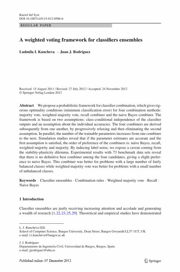
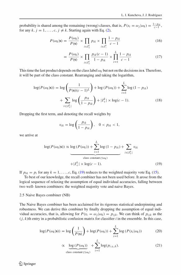
Fig. 2 Relationship between the ensemble accuracies using the majority vote as the benchmark combiner.Each scatterplot contains 4900 ensembles points

classifier are concatenated to form the final output of classifier i. L such classifiers weregenerated and the four combination rules were calculated. The classification accuracies foreach pair (L, c) were averaged across the 100 runs.

3.2 Results

Figure 2 shows the relationship between the combiners’ accuracies for the whole ranges ofL and c. Since there are 100 runs and 7 values of each parameter, there are 4900 ensembleaccuracies for each combiner. The figure shows that the weighted majority and the recallcombiner are similar, with the recall combiner having an edge over the WMV. They are bothbetter than the majority vote combiners and worse than Naive Bayes combiner.

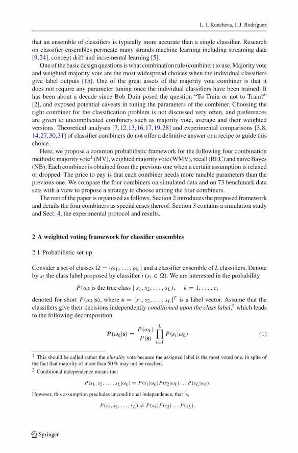
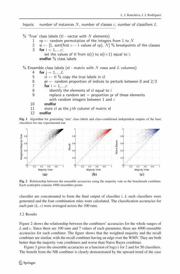
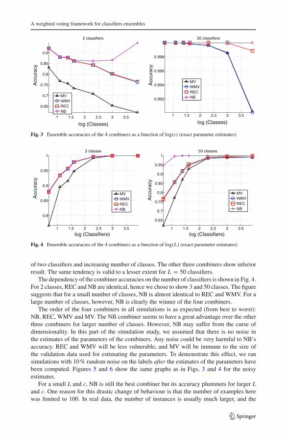
Figure 3 gives the ensemble accuracies as a function of log(c) for 2 and for 50 classifiers.The benefit from the NB combiner is clearly demonstrated by the upward trend of the case

123


1 1.5 2 2.5 3 3.5

0.65

0.7

0.75

0.8

0.85

0.9

log (Classes)

Acc

urac

y2 classifiers

MVWMVRECNB

1 1.5 2 2.5 3 3.5

0.992

0.994

0.996

0.998

1

log (Classes)

Acc

urac

y

50 classifiers

MVWMVRECNB

Fig. 3 Ensemble accuracies of the 4 combiners as a function of log(c) (exact parameter estimates)

1 1.5 2 2.5 3 3.5

0.8

0.85

0.9

0.95

1

log (Classifiers)

Acc

urac

y

3 classes

MVWMVRECNB

1 1.5 2 2.5 3 3.5

0.65

0.7

0.75

0.8

0.85

0.9

0.95

1

log (Classifiers)

Acc

urac

y50 classes

MVWMVRECNB

Fig. 4 Ensemble accuracies of the 4 combiners as a function of log(L) (exact parameter estimates)

of two classifiers and increasing number of classes. The other three combiners show inferiorresult. The same tendency is valid to a lesser extent for L = 50 classifiers.

The dependency of the combiner accuracies on the number of classifiers is shown in Fig. 4.For 2 classes, REC and NB are identical, hence we chose to show 3 and 50 classes. The figuresuggests that for a small number of classes, NB is almost identical to REC and WMV. For alarge number of classes, however, NB is clearly the winner of the four combiners.

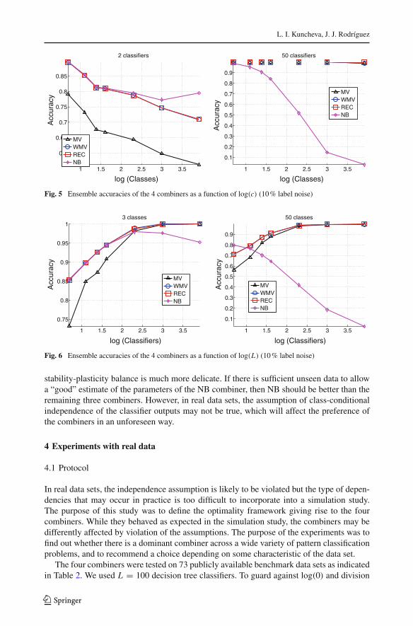
The order of the four combiners in all simulations is as expected (from best to worst):NB, REC, WMV and MV. The NB combiner seems to have a great advantage over the otherthree combiners for larger number of classes. However, NB may suffer from the curse ofdimensionality. In this part of the simulation study, we assumed that there is no noise inthe estimates of the parameters of the combiners. Any noise could be very harmful to NB’saccuracy. REC and WMV will be less vulnerable, and MV will be immune to the size ofthe validation data used for estimating the parameters. To demonstrate this effect, we ransimulations with 10 % random noise on the labels after the estimates of the parameters havebeen computed. Figures 5 and 6 show the same graphs as in Figs. 3 and 4 for the noisyestimates.

For a small L and c, NB is still the best combiner but its accuracy plummets for larger Land c. One reason for this drastic change of behaviour is that the number of examples herewas limited to 100. In real data, the number of instances is usually much larger, and the

123


1 1.5 2 2.5 3 3.5

0.6

0.65

0.7

0.75

0.8

0.85

log (Classes)

Acc

urac

y2 classifiers

MVWMVRECNB

1 1.5 2 2.5 3 3.5

0.1

0.2

0.3

0.4

0.5

0.6

0.7

0.8

0.9

log (Classes)

Acc

urac

y

50 classifiers

MVWMVRECNB

Fig. 5 Ensemble accuracies of the 4 combiners as a function of log(c) (10 % label noise)

1 1.5 2 2.5 3 3.5

0.75

0.8

0.85

0.9

0.95

1

log (Classifiers)

Acc

urac

y

3 classes

MVWMVRECNB

1 1.5 2 2.5 3 3.5

0.1

0.2

0.3

0.4

0.5

0.6

0.7

0.8

0.9

log (Classifiers)

Acc

urac

y50 classes

MVWMVRECNB

Fig. 6 Ensemble accuracies of the 4 combiners as a function of log(L) (10 % label noise)

stability-plasticity balance is much more delicate. If there is sufficient unseen data to allowa “good” estimate of the parameters of the NB combiner, then NB should be better than theremaining three combiners. However, in real data sets, the assumption of class-conditionalindependence of the classifier outputs may not be true, which will affect the preference ofthe combiners in an unforeseen way.

4 Experiments with real data

4.1 Protocol

In real data sets, the independence assumption is likely to be violated but the type of depen-dencies that may occur in practice is too difficult to incorporate into a simulation study.The purpose of this study was to define the optimality framework giving rise to the fourcombiners. While they behaved as expected in the simulation study, the combiners may bedifferently affected by violation of the assumptions. The purpose of the experiments was tofind out whether there is a dominant combiner across a wide variety of pattern classificationproblems, and to recommend a choice depending on some characteristic of the data set.

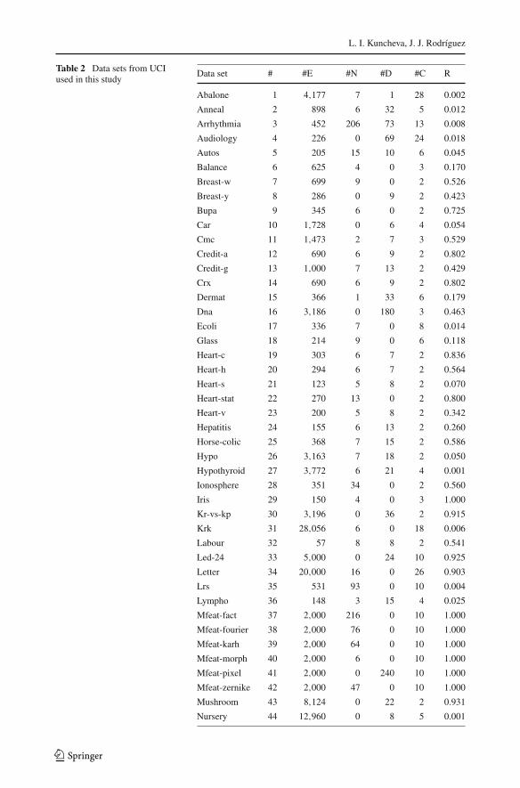
The four combiners were tested on 73 publicly available benchmark data sets as indicatedin Table 2. We used L = 100 decision tree classifiers. To guard against log(0) and division

123


by 0, we set a rounding threshold t = 10−8 for all classification accuracies, as well as for theestimates of the prior probabilities. All estimates which were less than t were reassigned to t,and all estimates greater than 1 − t were reset to 1 − t . For each scenario, we carried out10 replicas of 10-fold cross-validation. For each cross-validation fold, the training set wassplit into two equal parts called “proper” training and validation. All individual classifierswere trained on bootstrap samples from the proper training part and all parameters of thecombiners were evaluated on the validation part except for the prior probabilities which wereestimated from the whole training part of the fold.

All experiments were run within the Weka environment [10]. The accuracy of each ensem-ble is the average across the 100 testing results.

4.2 Results

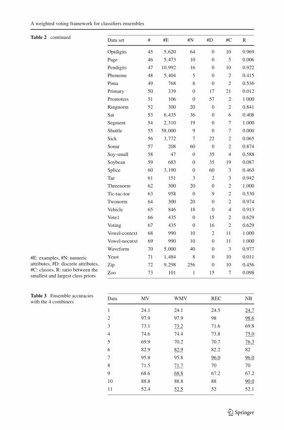
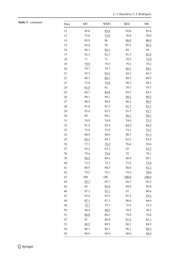
Table 3 shows the ensemble accuracies. The best accuracies for each data set are underlined.We have indicated the winner even where, due to rounding, the values for the data set appearas identical in the table. The bottom row of the table shows the average accuracies across thedata sets. With the diversity of domains and types of data sets in this experiment, and the largespan of classification accuracies, it is unlikely that these accuracies will be commensurable.But even though the average values across the data sets cannot serve as a valid performancegauge, they give a rough reference of the achievements of the combiners.

The table shows that there is no clear winner, hence we calculated the ranks for thecombiners. For example, on the dermatology data set, NB receives rank 1 (the best), RECreceives rank 2, WMV receives rank 3 and MV rank 4 (the worst). In case of a tie, the ranksare shared. The average ranks across the data sets were: MV 2.5205, WMV 2.4315, REC2.8356 and NB 2.2123, making NB the best combiner. The Friedman nonparametric ANOVAwas run on the ranks, followed by a multiple comparisons test. The p value of Friedman’sANOVA was 0.0269 indicating significant differences among the ranks. It was subsequentlyfound that NB is significantly better than REC. One possible reason for the poor performanceof REC is hinted by the simulation results. The results with REC are similar to these withWMV but the number of tunable parameters of REC is approximately c times larger. Withinaccurate estimates of the parameters, the small performance advantage of REC over WMVmay be smeared. In addition, it is not clear how the violation of the assumption of conditionalindependence affects the performance of the combiners. Then, it is not surprising the RECcombiner has not surfaced thus far.

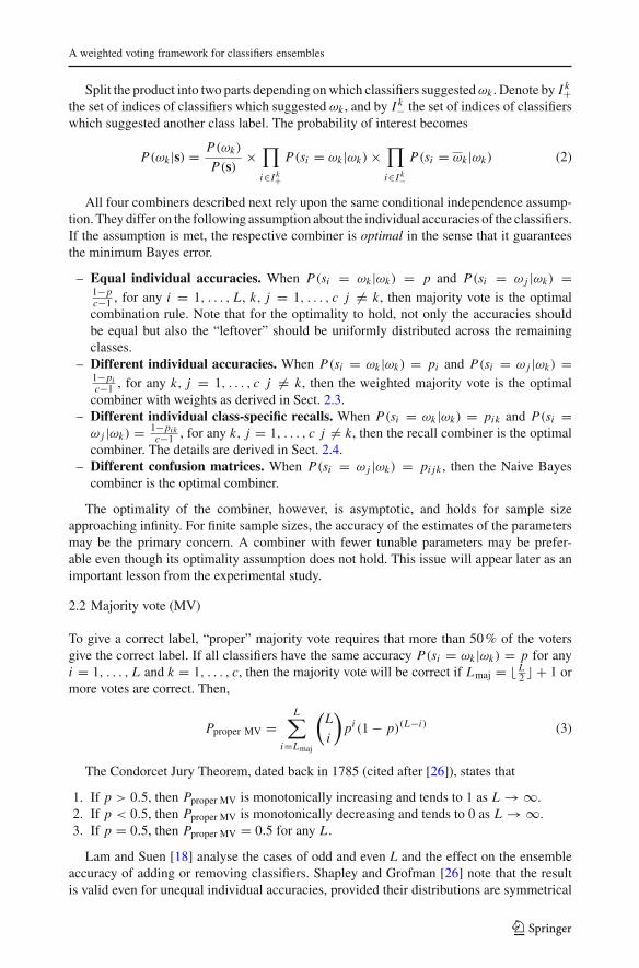
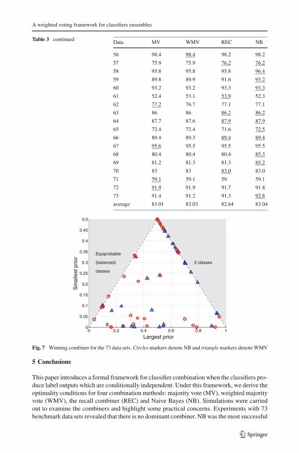
Figure 7 shows the distribution of the “winner” between NB and WMV, the combinerwith the second best rank. The axes are the prior of the largest class and the prior of thesmallest class. The feasible space is within a triangle, as shown in the figure. The right edgecorresponds to the 2-class problems because the smallest and the largest prior sum up to 1.The number of classes increases from this edge towards the origin (0, 0). The left edge of thetriangle corresponds to equiprobable classes. The largest prior on this edge is equal to thesmallest prior, which means that all classes have the same prior probabilities. This edge canbe thought of as the edge of balanced problems. The balance disappears towards the bottomright corner. The pinnacle of the triangle corresponds to two equiprobable classes.

Each data set is represented as a dot. The marker denotes the better combiner: circlesmarkers for NB and triangle markers for WMV. The figure does not shows a clear pattern ofdominance of one combiner over the other. NB seems to be slightly better for larger numberof classes and for generally balanced classes while WMV is better for problems with fewerunbalanced classes. If we applied the NB combiner for c > 3 and WMV for c ≤ 3 for the73 data sets, it will give average accuracy of 83.33 % and will achieve the top rank.

123


Table 2 Data sets from UCIused in this study

Data set # #E #N #D #C R

Abalone 1 4,177 7 1 28 0.002

Anneal 2 898 6 32 5 0.012

Arrhythmia 3 452 206 73 13 0.008

Audiology 4 226 0 69 24 0.018

Autos 5 205 15 10 6 0.045

Balance 6 625 4 0 3 0.170

Breast-w 7 699 9 0 2 0.526

Breast-y 8 286 0 9 2 0.423

Bupa 9 345 6 0 2 0.725

Car 10 1,728 0 6 4 0.054

Cmc 11 1,473 2 7 3 0.529

Credit-a 12 690 6 9 2 0.802

Credit-g 13 1,000 7 13 2 0.429

Crx 14 690 6 9 2 0.802

Dermat 15 366 1 33 6 0.179

Dna 16 3,186 0 180 3 0.463

Ecoli 17 336 7 0 8 0.014

Glass 18 214 9 0 6 0.118

Heart-c 19 303 6 7 2 0.836

Heart-h 20 294 6 7 2 0.564

Heart-s 21 123 5 8 2 0.070

Heart-stat 22 270 13 0 2 0.800

Heart-v 23 200 5 8 2 0.342

Hepatitis 24 155 6 13 2 0.260

Horse-colic 25 368 7 15 2 0.586

Hypo 26 3,163 7 18 2 0.050

Hypothyroid 27 3,772 6 21 4 0.001

Ionosphere 28 351 34 0 2 0.560

Iris 29 150 4 0 3 1.000

Kr-vs-kp 30 3,196 0 36 2 0.915

Krk 31 28,056 6 0 18 0.006

Labour 32 57 8 8 2 0.541

Led-24 33 5,000 0 24 10 0.925

Letter 34 20,000 16 0 26 0.903

Lrs 35 531 93 0 10 0.004

Lympho 36 148 3 15 4 0.025

Mfeat-fact 37 2,000 216 0 10 1.000

Mfeat-fourier 38 2,000 76 0 10 1.000

Mfeat-karh 39 2,000 64 0 10 1.000

Mfeat-morph 40 2,000 6 0 10 1.000

Mfeat-pixel 41 2,000 0 240 10 1.000

Mfeat-zernike 42 2,000 47 0 10 1.000

Mushroom 43 8,124 0 22 2 0.931

Nursery 44 12,960 0 8 5 0.001

123


Table 2 continued

#E: examples, #N: numericattributes, #D: discrete attributes,#C: classes, R: ratio between thesmallest and largest class priors

Data set # #E #N #D #C R

Optdigits 45 5,620 64 0 10 0.969

Page 46 5,473 10 0 5 0.006

Pendigits 47 10,992 16 0 10 0.922

Phoneme 48 5,404 5 0 2 0.415

Pima 49 768 8 0 2 0.536

Primary 50 339 0 17 21 0.012

Promoters 51 106 0 57 2 1.000

Ringnorm 52 300 20 0 2 0.841

Sat 53 6,435 36 0 6 0.408

Segment 54 2,310 19 0 7 1.000

Shuttle 55 58,000 9 0 7 0.000

Sick 56 3,772 7 22 2 0.065

Sonar 57 208 60 0 2 0.874

Soy-small 58 47 0 35 4 0.588

Soybean 59 683 0 35 19 0.087

Splice 60 3,190 0 60 3 0.463

Tae 61 151 3 2 3 0.942

Threenorm 62 300 20 0 2 1.000

Tic-tac-toe 63 958 0 9 2 0.530

Twonorm 64 300 20 0 2 0.974

Vehicle 65 846 18 0 4 0.913

Vote1 66 435 0 15 2 0.629

Voting 67 435 0 16 2 0.629

Vowel-context 68 990 10 2 11 1.000

Vowel-nocntxt 69 990 10 0 11 1.000

Waveform 70 5,000 40 0 3 0.977

Yeast 71 1,484 8 0 10 0.011

Zip 72 9,298 256 0 10 0.456

Zoo 73 101 1 15 7 0.098

Table 3 Ensemble accuracieswith the 4 combiners

Data MV WMV REC NB

1 24.1 24.1 24.5 24.7

2 97.9 97.9 98 98.6

3 73.1 73.2 71.6 69.8

4 74.6 74.4 73.8 75.0

5 69.9 70.2 70.7 76.3

6 82.9 82.9 82.2 82

7 95.8 95.8 96.0 96.0

8 71.5 71.7 70 70

9 68.6 68.8 67.2 67.2

10 88.8 88.8 88 90.0

11 52.4 52.5 52 52.1

123


Table 3 continued Data MV WMV REC NB

12 85.8 85.8 85.8 85.8

13 73.8 73.9 70.9 70.9

14 85.9 86 86.0 86.0

15 94.8 95 95.5 96.3

16 94.1 94.1 94 94

17 82.3 82.2 81.3 82.9

18 71 71 70.5 73.0

19 79.9 79.5 79.2 79.2

20 79.7 79.7 80.1 80.1

21 93.2 93.3 84.3 84.3

22 80.7 80.7 80.5 80.5

23 73.8 74.0 69.3 69.3

24 81.5 81 79.7 79.7

25 84.7 84.8 84.3 84.3

26 99.1 99.1 99.2 99.2

27 99.5 99.5 99.2 99.5

28 91.6 91.5 91.7 91.7

29 93.4 93.3 93.5 93.7

30 99 99.1 99.1 99.1

31 74.9 74.9 74.9 75.3

32 81.5 82.4 84.5 84.5

33 73.9 73.9 74.1 74.3

34 90.9 90.9 90.7 91.3

35 85.3 85.3 83.2 82.9

36 77.3 78.2 76.6 76.6

37 93.2 93.2 93 93.3

38 79.4 79.4 79 79.1

39 89.5 89.4 89.4 89.1

40 72.3 72.3 72.5 73.0

41 80.5 80.5 80.6 81.2

42 75.2 75.1 74.4 78.0

43 100 100 100.0 100.0

44 95.7 95.7 94.7 95.3

45 95 95.0 94.9 95.0

46 97.1 97.1 97 96.8

47 97.5 97.5 97.5 97.6

48 87.1 87.1 86.6 86.6

49 75.7 75.7 75.5 75.5

50 40.4 40.5 39.9 38.3

51 80.8 80.2 79.8 79.8

52 87 86.8 87.1 87.1

53 89.5 89.5 89.1 88.9

54 96.1 96.1 96.1 96.4

55 99.9 99.9 99.9 99.9

123


Table 3 continued Data MV WMV REC NB

56 98.4 98.4 98.2 98.2

57 75.9 75.9 76.2 76.2

58 95.8 95.8 95.8 96.4

59 89.8 89.9 91.6 93.2

60 93.2 93.2 93.3 93.3

61 52.4 53.1 53.9 52.3

62 77.2 76.7 77.1 77.1

63 86 86 86.2 86.2

64 87.7 87.6 87.9 87.9

65 72.4 72.4 71.6 72.5

66 89.4 89.3 89.4 89.4

67 95.6 95.5 95.5 95.5

68 80.4 80.4 80.4 85.3

69 81.2 81.3 81.3 85.2

70 83 83 83.0 83.0

71 59.1 59.1 59 59.1

72 91.9 91.9 91.7 91.8

73 91.4 91.2 91.3 92.8

average 83.01 83.03 82.64 83.04

0 0.2 0.4 0.6 0.8 10

0.05

0.1

0.15

0.2

0.25

0.3

0.35

0.4

0.45

0.5

Equiprobable

(balanced)

classes

2 classes

Largest prior

Sm

alle

st p

rior

Fig. 7 Winning combiner for the 73 data sets. Circles markers denote NB and triangle markers denote WMV

5 Conclusions

This paper introduces a formal framework for classifier combination when the classifiers pro-duce label outputs which are conditionally independent. Under this framework, we derive theoptimality conditions for four combination methods: majority vote (MV), weighted majorityvote (WMV), the recall combiner (REC) and Naive Bayes (NB). Simulations were carriedout to examine the combiners and highlight some practical concerns. Experiments with 73benchmark data sets revealed that there is no dominant combiner. NB was the most successful

123


combiner overall but the differences with MV and WMV were not found to be statisticallysignificant. NB has the widest optimality scope but also the largest number of parametersto train among the four combiners. The simulation study showed that NB can suffer badlyfrom inaccurate estimates of its parameters. The experimental results with real data did notshow such anomalies with NB, suggesting that, in practice, the data are usually sufficient forobtaining reasonable parameter estimates.

The differences between the performances of the four combiners in the simulation studywere blurred in the experiments with real data for at least two reasons. Beside the noise ofparameter estimates, the second reason for this is that the conditional independence assump-tion may not be satisfied. It would be interesting to study to what extent this assumptionholds, and how it affects the combiners. Another direction for future research is how thecombiners are influenced by: the choice of base classifier, the ensemble sizes, the methodof producing the base classifiers and the ensemble diversity. It is also interesting to exploreother characteristics of the data sets and find better niches for the four combiners.

References

1. Brown G (2010) Ensemble learning. In: Sammut C, Webb G (eds) In encyclopedia of machine learning.Springer, Berlin

2. Duin RPW (2002) The combining classifier: to train or not to train? In: Proceedings 16th internationalconference on pattern recognition, ICPR’02, Canada, pp. 765–770

3. Duin RPW, Tax DMJ (2000) Experiments with classifier combination rules. In: Kittler J, Roli F (eds)Multiple classifier systems, vol. 1857 of lecture notes in computer science. Springer, Italy, pp. 16–29

4. Eibl G, Pfeiffer KP (2005) Multiclass boosting for weak classifiers. J Mach Learn Res 6:189–2105. Elwell R, Polikar R (2011) Incremental learning of concept drift in nonstationary environments. IEEE

Trans Neural Netw 22(10):1517–15316. Freund Y, Schapire RE (1996) Experiments with a new boosting algorithm. Thirteenth international

conference on machine learning. Morgan Kaufmann, San Francisco, pp. 148–1567. Fumera G, Roli F (2005) A theoretical and experimental analysis of linear combiners for multiple classifier

systems. IEEE Trans Pattern Anal Mach Intell 27:942–9568. Ghosh K, Ng YS, Srinivasan R (2011) Evaluation of decision fusion strategies for effective collaboration

among heterogeneous fault diagnostic methods. Comput Chem Eng 35(2):342–3559. Grossi V, Turini F (2012) Stream mining: a novel architecture for ensemble-based classification. Knowl

Inf Syst 30:247–28110. Hall M, Frank E, Holmes G, Pfahringer B, Reutemann P, Witten IH (2009) The WEKA data mining

software: An update, SIGKDD explorations 1111. Kim H, Kim H, Moon H, Ahn H (2011) A weight-adjusted voting algorithm for ensembles of classifiers.

J Korean Stat Soc 40(4):437–44912. Kittler J, Hatef M, Duin RPW, Matas J (1998) On combining classifiers. IEEE Trans Pattern Anal Mach

Intell 20(3):226–23913. Kuncheva L (2002) A theoretical study on six classifier fusion strategies. IEEE Trans Pattern Anal Mach

Intell 24(2):281–28614. Kuncheva LI (2003) ‘Fuzzy’ vs ‘non-fuzzy’ in combining classifiers designed by boosting. IEEE Trans

Fuzzy Syst 11(6):729–74115. Kuncheva LI (2004) Combining pattern classifiers. Methods and algorithms. Wiley, New York16. Kuncheva L, Whitaker C, Shipp C, Duin R (2003) Limits on the majority vote accuracy in classifier

fusion. Pattern Anal Appl 6:22–3117. Lam L, Suen C (1995) Optimal combination of pattern classifiers. Pattern Recognit Lett 16:945–95418. Lam L, Suen C (1997) Application of majority voting to pattern recognition: an analysis of its behavior

and performance. IEEE Trans Syst Man Cybern 27(5):553–56819. Lin X, Yacoub S, Burns J, Simske S (2003) Performance analysis of pattern classifier combination by

plurality voting. Pattern Recognit Lett 24(12):1795–196920. Lingenfelser F, Wagner J, André E (2011) A systematic discussion of fusion techniques for multi-modal

affect recognition tasks. In: Proceedings of the 13th international conference on multimodal interfaces,ICMI ’11. ACM, New York, pp. 19–26

123


21. Matan O (1996) On voting ensembles of classifiers (extended abstract). In: Proceedings of AAAI-96workshop on integrating multiple learned models, pp. 84–88

22. Polikar R (2006) Ensemble based systems in decision making. IEEE Circuits Syst Mag 6:21–4523. Re M, Valentini G, (2011) Ensemble methods: a review, Data mining and machine learning for astronom-

ical applications, Chapman & Hall, London (in press)24. Read J, Bifet A, Holmes G, Pfahringer B (2012) Scalable and efficient multi-label classification for

evolving data streams. Mach Learn 88(1–2, SI):243–27225. Sewell M (2011) Ensemble learning, Technical Report RN/11/02. Department of Computer Science,

UCL, London26. Shapley L, Grofman B (1984) Optimizing group judgemental accuracy in the presence of interdependen-

cies. Public Choice 43:329–34327. Tax DMJ, Duin RPW, van Breukelen M (1997) Comparison between product and mean classifier combi-

nation rules. In: Proceedings workshop on statistical pattern recognition, Prague, Czech Republic28. Tumer K, Ghosh J (1999) Combining artificial neural nets. In: Sharkey A (ed) Linear and order statistics

combiners for pattern classification. Springer, London, pp 127–16129. Xu L, Krzyzak A, Suen CY (1992) Methods of combining multiple classifiers and their application to

handwriting recognition. IEEE Trans Syst Man Cybern 22:418–43530. Zhang CX, Duin RP (2011) An experimental study of one- and two-level classifier fusion for different

sample sizes. Pattern Recognit Lett 32(14):1756–176731. Zhang L, Zhou WD (2011) Sparse ensembles using weighted combination methods based on linear

programming. Pattern Recognit 44(1):97–106

Author Biographies

Ludmila I. Kuncheva received the MSc degree from the TechnicalUniversity of Sofia, Bulgaria in 1982, and the Ph.D. degree from theBulgarian Academy of Sciences in 1987. Until 1997, she worked at theCentral Laboratory of Biomedical Engineering at the Bulgarian Acad-emy of Sciences. She is currently a Professor at the School of Com-puter Science, Bangor University, UK. Her interests include patternrecognition and classification, machine learning and classifier ensem-bles. She has published two books and above 200 scientific papers.

Juan J. Rodríguez received the BS, MS and Ph.D. degrees inComputer Science from the University of Valladolid, Spain, in 1994,1998 and 2004, respectively. He worked with the Department of Com-puter Science, University of Valladolid from 1995 to 2000. Currently,he is working with the Department of Civil Engineering, Universityof Burgos, Spain, where he is an Associate Professor. His main inter-ests are machine learning, data mining and pattern recognition. He is amember of the IEEE Computer Society.

123

Documents

A Weighted Voting Framework for Classifiers Ensembles