A Weighted Additive Model for Comparative Analysis on

International Journal of Industrial Engineering and Operations Management (IJIEOM) Volume. 2, No. 1, October 2020

© IEOM Society International

IEOM Society International

International Journal of Industrial Engineering

and Operations Management (IJIEOM) Volume 2, No. 1, October 2020

pp. 42 - 62

A Weighted Additive Model for Comparative Analysis on Demand Factors among Multiple Seasonal Products: Nationwide Demand of

Japanese Alcoholic Beverages

Tsuyoshi Kurihara Certified and Accredited Meteorologist

Hiroshima, Japan [email protected]

Takaaki Kawanaka

Institute for Innovation in International Engineering Education, Graduate School of Engineering The University of Tokyo

7-3-1 Hongo, Bunkyo-ku, Tokyo, Japan [email protected]

Hiroshi Yamashita

Department of Commerce, Meiji University 1-1 Kanda-Surugadai, Chiyoda-ku, Tokyo, Japan

[email protected] https://doi.org/10.46254/j.ieom.20200104

ABSTRACT

The climate has recently been fluctuating globally. Such climate, which affects the demand for seasonal products, varies depending on geographical conditions. However, analysis models of previous studies on nationwide demand for seasonal products have not considered differences in climate attributed to different regions in the country. Therefore, in this study, focusing on the relationship between climate and region, we extract common characteristics on the nationwide demand factors for a seasonal product group (Japanese alcoholic beverages). We propose a new demand analysis model that enables a comparative analysis among multiple items, more accurately, cross-sectionally, and concisely by using two independent factors: meteorological factors by item and regional weights (demand). We develop a new algorithm using alternating least squares for the estimation problem of inseparable parameters generated by expressing these two factors in the form of products. The validity and effectiveness of the proposed model and algorithm were confirmed by empirical analysis using public data. This makes it possible to theoretically consider regional differences (climate and demand) for nationwide demand of seasonal products. Consequently, the proposed model can be used to conduct multifaceted analysis to situation changes such as climate fluctuations to realize effective sales and operation planning of seasonal products.

ARTICLE INFO

Received December 30, 2019 Received in revised

form June 30, 2020

Accepted July 11, 2020

KEYWORDS Seasonal dependency, Meteorological factor, Regional difference,

Inseparable parameter, Alternating least squares method

42



1. Introduction The global climate change has recently intensified, leading to increased fluctuations in regional climate compared to typical seasonal trends. For example, Japan’s highest mean temperature since 1898 was in the summer of 2010 (JMA 2010), according to the Japan Meteorological Agency's (JMA) historical records. Only two years later, in the winter of 2012, the mean temperature in eastern and western Japan fell below normal (defined as the mean temperature over the past 30 years) for three consecutive months, for the first time in 26 years (JMA 2012). Such climate fluctuations have resulted in more severe seasonal changes in Japan, where the four seasons are distinct; this greatly influences seasonal products, such as beer and home air conditioners, whose demand fluctuates depending on the climate. Demand seems to be affected not only by the usual seasonal changes (represented by mean values) but also by climate fluctuations that exceed the usual seasonal changes. The manufacturing industry has experienced major changes in the market environment in recent years. The consistent manufacture and supply of products at a low cost, without missing sale opportunities, has become a significant issue. This poses a more difficult issue for companies that manufacture seasonal products with large demand fluctuations. From the aspect of supply and demand management, two problems need to be addressed: (A) how to appropriately analyze demand factors and accurately predict demand and (B) how to level production while lowering inventory without missing sales opportunities. In sales and operation planning (S & OP), which fulfills the planning function of supply and demand management (Bowersox et al. 2010), problem (A) can be regarded as an accuracy problem of demand analysis and forecasting. In contrast, problem (B) can be treated as a production quantity planning problem of aggregate production planning that must be solved for each production quantity per unit period (e.g., per month) throughout the planning horizon (Kuroda 1994). As the highest-level planning, S & OP requires not only short processing time for subsequent production and procurement planning that takes time but also multifaceted analysis in which various situation changes for management decision support must be assumed. In general, the models used for demand analysis and forecasting can be broadly divided into regression and time series models (Makridakis et al. 1998; Sanders 2000; Honda 2000). Regression models analyze demand based on causal relationships with explanatory variables and time series models analyze demand based on past demand fluctuation patterns. We previously proposed that the demand for a seasonal product is strongly influenced by the climate at its time of sale (referred to as “seasonal dependency” (Kurihara et al. 2018)); from this consistent perspective, we have aimed to develop a more appropriate demand analysis model for seasonal products, based on a regression model. An understanding of the demand factors of seasonal products and their structure is required as the basis of the regression model. Therefore, our previous studies (Kurihara and Yamashita 2012; Kurihara et al. 2019) analyzed the characteristics related to demand factors, based on the geography and climate of Japan and the nationality and regionality of the Japanese people. For characteristics related to seasonal dependency, we first determined the climate characteristics: (1) the climate varies from region to region (referred to as “regional characteristics of climate”). Under the condition of (1), we subsequently proposed two characteristics of the demand factors for a Japanese seasonal product: (2) the demand fluctuates due to climate (original “seasonal dependency”) but (3) the impact of meteorological factors on demand does not change across different regions, if the climate remains the same (referred to as “regional homogeneity of meteorological factors”). For characteristics other than seasonal dependency, we further proposed a characteristic of the relationship between region and nationwide demand: (4) the regional impact on nationwide demand (regional weight) varies by region (referred to as “regional differences in demand”). In order to structurally and concisely replicate the relationship between nationwide demand, factors, and regions based on these characteristics, we proposed two nationwide demand analysis models that include regional differences in demand; a model for home air conditioners (Kurihara and Yamashita 2012) and beer (Kurihara et al. 2019). However, these models are regression models for a single item that aim at accurate analysis of the demand factors for individual seasonal products. Performing cross-sectional and concise analysis of the nationwide demand factors for multiple items in a seasonal product group with these models will be difficult. The models proposed by Mirasgedis et al. (2014) and Ramanathan and Muyldermans (2010) are regression models for beverages capable of analyzing the nationwide demand factors of seasonal products among multiple items. However, they cannot consider regional characteristics of climate and regional differences in demand as their models represent meteorological factors in the climate of only one region. The models by Cabral et al. (2019) and Kotler and Keller (2015) can consider regional characteristics of climate and regional differences in demand. However, they cannot analyze the impact of meteorological factors on nationwide demand based on the regional homogeneity of meteorological factors. In this study, we first examined the characteristics of demand factors common within a seasonal product group based on our previous study (Kurihara et al. 2019). We focused on six major alcoholic beverages in Japan (beer, happoshu (a beer-like beverage), sake (Japanese rice wine), wine, shochu (Japanese spirits), and whiskey) as a typical seasonal product group. In addition to the above four characteristics related to the demand factors of a seasonal product, two further

43



characteristics of the demand factors of a seasonal product group were introduced: (5) the impact of demand factors varies by item (referred to as “item differences in demand factors”) and (6) regional differences in demand (regional weight) do not change in the same region, even in different items (referred to as “item homogeneity of regional differences”). Based on these six characteristics related to demand factors, we attempted to structurally capture the relationship between nationwide demand, demand factors, and regions and reproduce it for a seasonal product group. This enabled a comparative analysis of demand factors with separation of seasonal dependency and regional differences in demand, in the case of multiple items. Thus, we constructed a new model that expresses mutually independent meteorological factors by item and regional weights common to the items as products and other factors (social customs, policy, and trend) for each item as sums, based on the demand analysis model of Kurihara et al. (2019). To estimate the “inseparable” parameters (Takane 1976) by the product of mutually independent parameters, we developed a new algorithm using the alternating least squares method (Takane et al. 1980), based on our previous study (Kurihara et al. 2019). Moreover, we conducted empirical analysis using nationwide demand data for six alcoholic beverages (monthly data from the Family Income and Expenditure Survey: Statistics Bureau, Japan 2010–2015) and meteorological data (air temperature and precipitation) for three regions in Japan (JMA 2010–2015). Both sets of data are available to the public and easy to use. Based on the results, we verified the validity and effectiveness of the proposed model and algorithm and obtained useful knowledge about the demand of the six alcoholic beverages. If the proposed model is applied to the S & OP process of a seasonal product manufacturer, it is possible to easily perform a multifaceted analysis on the nationwide demand factors for a seasonal product group via a single model by assuming various situation changes (e.g., climate fluctuations). Consequently, it is possible to provide useful suggestions for sales planning for similar competing products, support efficient production preparation for the products in aggregate production planning, and contribute to timely and appropriate management decision making. Utilizing the proposed algorithm, the solution of the proposed model can be calculated via the standard tool Excel; hence, it can be applied to small and medium enterprises (SMEs). 2. Literature overview 2.1 Viewpoints of demand analysis In general, demand analysis models are broadly categorized into regression and time series models (Makridakis et al. 1998; Sanders 2000; Honda 2000). Regression models include single regression analysis and multiple regression analysis (linear regression model and nonlinear regression model). Time series models include the TCSI decomposition method (moving average and CENSUS method), exponential smoothing (Holtz method and Holtz-Winter method), and the autoregressive model (ARMA model, Box-Jenkins method, and Kalman filter method). For the demand analysis of foods and beverages including alcoholic beverages, which is the subject of this study, various recent studies have been conducted mainly focusing on time series models. Examples of such time series models include the TCSI decomposition model by Tirkes et al. (2017), the Holz–Winter model by Barbosa et al. (2015), the ARIMA models by Lenten et al. (1999) and Veiga et al. (2014), and the S-ARIMA model by Mircetic et al. (2016). In particular, the model by Mircetic et al. (2016) considers seasonal fluctuations in freight flows in a beverage supply chain; ultimately, these are models in which demand is analyzed via past demand fluctuation patterns. In recent years, the climate has begun to dynamically change beyond what has previously been seen. The climate has a large impact on demand for seasonal products. Given these environmental changes, regression models capable of reflecting changes in climate may be more accurate than time series models that rely solely on past demand fluctuation patterns when analyzing demand for seasonal products. We take the perspective of seasonal dependency (Kurihara and Yamashita 2012; Kurihara et al. 2019), that is, “the demand for seasonal products is strongly influenced by the climate (e.g., air temperature and precipitation) at the time when they are sold, rather than the fluctuation patterns of past demands.” From this perspective, we thus determined to develop a more accurate and appropriate demand analysis model for seasonal products, based on a regression model; to do so, an understanding of the demand factors of seasonal products and their structures is required. Therefore, we analyzed the characteristics related to demand factors with respect to the heterogeneity and homogeneity of demand factors, based on the geography and climate of Japan and the nationality and regionality of the Japanese people. For characteristics related to seasonal dependency, we first demonstrated the climate characteristics: (1) the climate affecting demand varies from region to region (regional characteristics of climate) as Japan is geographically located in the mid-latitude and is elongated from north to south. Under the condition of (1), we subsequently proposed two characteristics of a Japanese seasonal product’s demand factors: (2) the demand fluctuates due to climate (original seasonal dependency), however, (3) the impact of meteorological factors on demand does not change in the same climate even in different regions (regional homogeneity of meteorological factors), based on the

44



relatively homogeneous nationality of the Japanese people. For characteristics other than seasonal dependency, we further indicated characteristics of the relationship between region and nationwide demand: (4) the regional impact on nationwide demand (regional weight) varies by region (regional differences in demand), depending on the population, economic power, etc. of the region. Summarizing these four characteristics related to demand factors, it is suggested that the climate varies with region; however, the meteorological factors themselves do not vary depending on the region and are independent of regional weights. For home air conditioners (a seasonal durable product), we proposed a regression model with regional differences, focusing on meteorological factors and regional weights (Kurihara and Yamashita 2012). The model expresses the impact of regional climate fluctuations on nationwide demand as products of mutually independent meteorological factors and regional weights. With regard to beer (a seasonal nondurable product), we proposed a regression model with regional differences to further improve the accuracy of our analysis model for home air conditioners (Kurihara et al. 2019). The model considers the sum of the social customs, policy, and trend factors, in addition to the main factors of meteorological factors and regional weights. However, both models are demand analysis models for the individual seasonal product. With regard to both models, it is difficult to compare and analyze the differences in the demand factors for multiple items within a seasonal product group, in a cross-sectional and concise manner. 2.2 Analysis methods in the field of beverage and food consumption Nakatani (2012), Lenten and Moosa (1999), Moosa and Baxter (2002), Mirasgedis et al. (2014), Ramanathan and Muyldermans (2010), Keleş et al. (2018), and others have proposed comparative analysis models among multiple items pertaining to nationwide demand for seasonal products, particularly alcoholic beverages, drinks, and food. The model developed by Nakatani (2012) is a nonlinear (logarithmic) regression model for beer and happoshu. It compares and analyzes demand factors (seasons, prices, and incomes), based on quarterly demand fluctuations, under the condition of competing items. However, it cannot be used to analyze demand factors (seasonal dependency) at the monthly level required in S & OP, because the model considers demand factors in a quarterly period. The model proposed by Lenten and Moosa (1999) is a time series (autoregressive) model for beer, wine, and distilled alcohol; it compares and analyzes demand factors at the seasonal level, based on quarterly demand fluctuation. The model developed by Moosa and Baxter (2002) is a time series (autoregressive) model using the Kalman filter method for beer and wine; this compares and analyzes demand factors (seasons, trends, and prices), based on quarterly demand fluctuations. However, these models cannot also be used to analyze the seasonal demand fluctuations (seasonal dependency) in a monthly time frame owing to the quarterly units, similar to Nakatani’s model. In contrast, the model presented by Mirasgedis et al. (2014) is a nonlinear (logarithmic) regression model for drinking water (carbonated and noncarbonated) and nonalcoholic beverages (soft drinks and juice). This model is capable of comparing and analyzing demand factors (climate, social customs, and trend) based on monthly fluctuations in the whole demand. However, this model does not consider regional characteristics of climate and regional differences in demand as it represents the meteorological factors by the climate of only one region (referred to as a “one-region representative model”). The model by Ramanathan and Muyldermans (2010) is a structural equation model (SEM) for soft drinks. It can be used to analyze the relationship and structure of factors related to weekly fluctuations in the whole demand and to compare and analyze factors among multiple items. However, the model cannot also consider regional characteristics of climate and regional differences in demand, because it is a one-region representative model like that of Mirasgedis et al. (2014). The model proposed by Keleş et al. (2018) is a two-stage economic model for long-term and short-term fluctuations of six beverage items in 52 states of the United States. With regard to short-term fluctuations, this model can capture regional characteristics of climate and regional differences in demand, after collating states into regions via a latent class regression model. However, it cannot capture regional characteristics of climate and regional differences in demand as both demand and climate are combined into one (the whole country), when analyzing nationwide demand. In recent years, studies on hybrid time series and regression models that consider meteorological factors have been conducted by Bratina and Faganel (2008) and Arunraj and Ahrens (2015) to further improve analysis accuracy. However, they cannot also consider regional characteristics of climate and regional differences in demand as they are all one-region representative models. 2.3 Analysis methods in other fields Expanding the scope of the study on seasonal products to fields other than beverage and food consumption, there is a study by Apadula et al. (2012) in the field of electricity consumption. The study developed a multiple regression analysis model using meteorological and socio-economic factors to analyze the monthly electricity demand in Italy. However, the meteorological data collected for each region are combined when analyzing the relationship between nationwide demand and climate; therefore, not only regional differences in demand but also regional characteristics of climate are

45



not considered. Next, in the field of water consumption, a study by Cabral et al. (2019) proposed a model for making water demand scenarios in Portugal. This model combines a multiple regression model for analyzing the relationship between water demand and climate by region and a scenario planning (long-term, medium-term, and short-term) approach. It can analyze demand by region based on the regional characteristics of climate. However, the impact of meteorological factors may change between different regions, even if the climate is the same. In other words, it cannot consider regional homogeneity of meteorological factors. Regardless of the field, there is a regional demand accumulation model (accumulation method by market) by Kotler and Keller (2015), which uses a typical method of considering regional characteristics of climate and differences in demand. This is a method of accumulating the demand in each region to construct nationwide demand based on a multiple regression analysis model that relates meteorological factors and demand for each region. However, this method cannot consider the regional homogeneity of meteorological factors and cannot concisely perform a comparative analysis among multiple items in a single model, similar to the model by Cabral et al. (2019). 2.4 Comparison analysis of demand factors between Japan and other countries To examine the commonality of demand factors across countries, we compare the demand factors extracted for Japanese beer with those of seasonal products in other countries. Fogarty (2010) analyzed the consumption by country by classifying alcoholic beverages into beer, wine, and spirits; according to this study, beer has the highest consumption; one of the countries with the highest beer consumption is the United States. The United Kingdom, Germany, Australia, New Zealand, Japan, etc. (except the United States) have a high beer consumption ratio and regional characteristics of climate. These countries are located in the mid-latitudes and are long in the north and south. Thus, we compared the study by Beer Industry Electronic Commerce Coalition (BIECC) (2009) in the United States and the study by Kurihara et al. (2019) in Japan. Table 1 presents a comparison of the demand factors by classifying them into two categories: major factors and minor sub-factors.

46



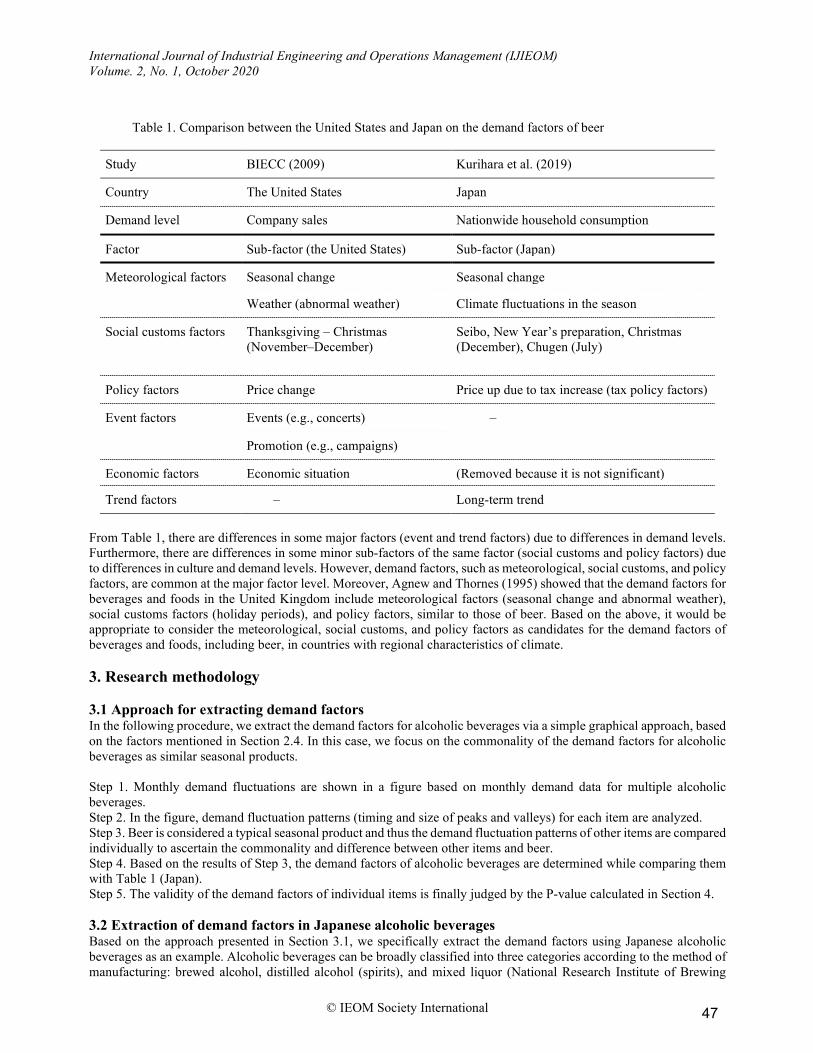
Table 1. Comparison between the United States and Japan on the demand factors of beer

Study BIECC (2009) Kurihara et al. (2019)

Country The United States Japan

Demand level Company sales Nationwide household consumption

Factor Sub-factor (the United States) Sub-factor (Japan)

Meteorological factors Seasonal change Seasonal change

Weather (abnormal weather) Climate fluctuations in the season

Social customs factors Thanksgiving – Christmas (November–December)

Seibo, New Year’s preparation, Christmas (December), Chugen (July)

Policy factors Price change Price up due to tax increase (tax policy factors)

Event factors Events (e.g., concerts) –

Promotion (e.g., campaigns)

Economic factors Economic situation (Removed because it is not significant) Trend factors – Long-term trend

From Table 1, there are differences in some major factors (event and trend factors) due to differences in demand levels. Furthermore, there are differences in some minor sub-factors of the same factor (social customs and policy factors) due to differences in culture and demand levels. However, demand factors, such as meteorological, social customs, and policy factors, are common at the major factor level. Moreover, Agnew and Thornes (1995) showed that the demand factors for beverages and foods in the United Kingdom include meteorological factors (seasonal change and abnormal weather), social customs factors (holiday periods), and policy factors, similar to those of beer. Based on the above, it would be appropriate to consider the meteorological, social customs, and policy factors as candidates for the demand factors of beverages and foods, including beer, in countries with regional characteristics of climate. 3. Research methodology 3.1 Approach for extracting demand factors In the following procedure, we extract the demand factors for alcoholic beverages via a simple graphical approach, based on the factors mentioned in Section 2.4. In this case, we focus on the commonality of the demand factors for alcoholic beverages as similar seasonal products. Step 1. Monthly demand fluctuations are shown in a figure based on monthly demand data for multiple alcoholic beverages. Step 2. In the figure, demand fluctuation patterns (timing and size of peaks and valleys) for each item are analyzed. Step 3. Beer is considered a typical seasonal product and thus the demand fluctuation patterns of other items are compared individually to ascertain the commonality and difference between other items and beer. Step 4. Based on the results of Step 3, the demand factors of alcoholic beverages are determined while comparing them with Table 1 (Japan). Step 5. The validity of the demand factors of individual items is finally judged by the P-value calculated in Section 4. 3.2 Extraction of demand factors in Japanese alcoholic beverages Based on the approach presented in Section 3.1, we specifically extract the demand factors using Japanese alcoholic beverages as an example. Alcoholic beverages can be broadly classified into three categories according to the method of manufacturing: brewed alcohol, distilled alcohol (spirits), and mixed liquor (National Research Institute of Brewing

47



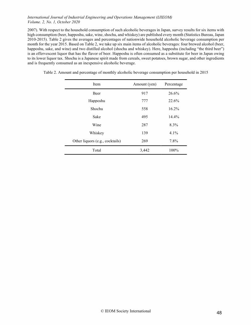
2007). With respect to the household consumption of such alcoholic beverages in Japan, survey results for six items with high consumption (beer, happoshu, sake, wine, shochu, and whiskey) are published every month (Statistics Bureau, Japan 2010-2015). Table 2 gives the averages and percentages of nationwide household alcoholic beverage consumption per month for the year 2015. Based on Table 2, we take up six main items of alcoholic beverages: four brewed alcohol (beer, happoshu, sake, and wine) and two distilled alcohol (shochu and whiskey). Here, happoshu (including “the third beer”) is an effervescent liquor that has the flavor of beer. Happoshu is often consumed as a substitute for beer in Japan owing to its lower liquor tax. Shochu is a Japanese spirit made from cereals, sweet potatoes, brown sugar, and other ingredients and is frequently consumed as an inexpensive alcoholic beverage.

Table 2. Amount and percentage of monthly alcoholic beverage consumption per household in 2015

Item Amount (yen) Percentage

Beer 917 26.6% Happoshu 777 22.6%

Shochu 558 16.2% Sake 495 14.4% Wine 287 8.3%

Whiskey 139 4.1% Other liquors (e.g., cocktails) 269 7.8%

Total 3,442 100%

48



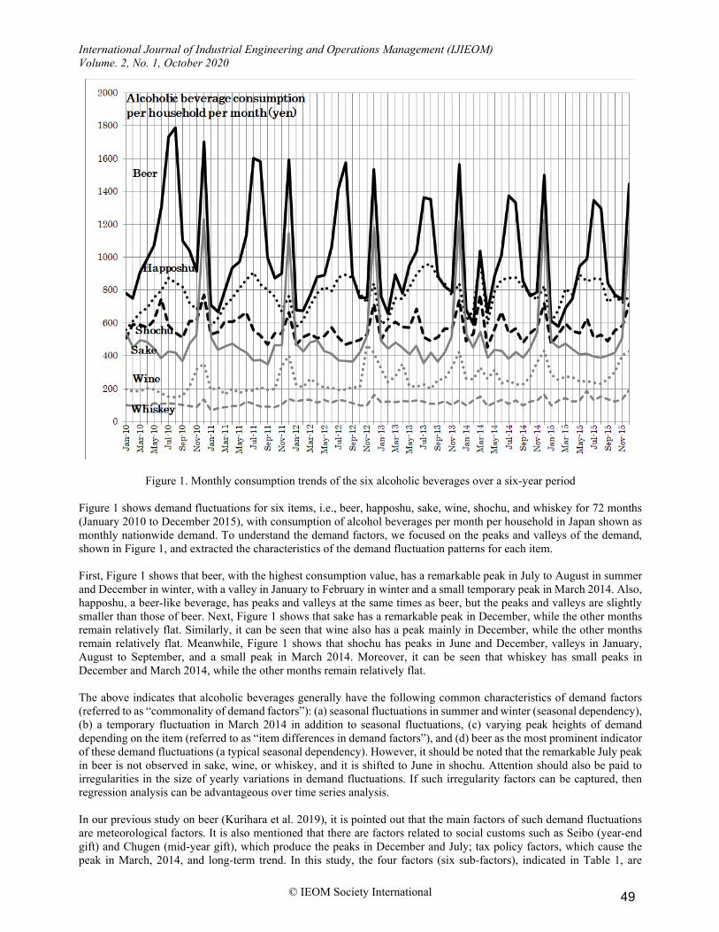
Figure 1. Monthly consumption trends of the six alcoholic beverages over a six-year period Figure 1 shows demand fluctuations for six items, i.e., beer, happoshu, sake, wine, shochu, and whiskey for 72 months (January 2010 to December 2015), with consumption of alcohol beverages per month per household in Japan shown as monthly nationwide demand. To understand the demand factors, we focused on the peaks and valleys of the demand, shown in Figure 1, and extracted the characteristics of the demand fluctuation patterns for each item. First, Figure 1 shows that beer, with the highest consumption value, has a remarkable peak in July to August in summer and December in winter, with a valley in January to February in winter and a small temporary peak in March 2014. Also, happoshu, a beer-like beverage, has peaks and valleys at the same times as beer, but the peaks and valleys are slightly smaller than those of beer. Next, Figure 1 shows that sake has a remarkable peak in December, while the other months remain relatively flat. Similarly, it can be seen that wine also has a peak mainly in December, while the other months remain relatively flat. Meanwhile, Figure 1 shows that shochu has peaks in June and December, valleys in January, August to September, and a small peak in March 2014. Moreover, it can be seen that whiskey has small peaks in December and March 2014, while the other months remain relatively flat. The above indicates that alcoholic beverages generally have the following common characteristics of demand factors (referred to as “commonality of demand factors”): (a) seasonal fluctuations in summer and winter (seasonal dependency), (b) a temporary fluctuation in March 2014 in addition to seasonal fluctuations, (c) varying peak heights of demand depending on the item (referred to as “item differences in demand factors”), and (d) beer as the most prominent indicator of these demand fluctuations (a typical seasonal dependency). However, it should be noted that the remarkable July peak in beer is not observed in sake, wine, or whiskey, and it is shifted to June in shochu. Attention should also be paid to irregularities in the size of yearly variations in demand fluctuations. If such irregularity factors can be captured, then regression analysis can be advantageous over time series analysis. In our previous study on beer (Kurihara et al. 2019), it is pointed out that the main factors of such demand fluctuations are meteorological factors. It is also mentioned that there are factors related to social customs such as Seibo (year-end gift) and Chugen (mid-year gift), which produce the peaks in December and July; tax policy factors, which cause the peak in March, 2014, and long-term trend. In this study, the four factors (six sub-factors), indicated in Table 1, are

49



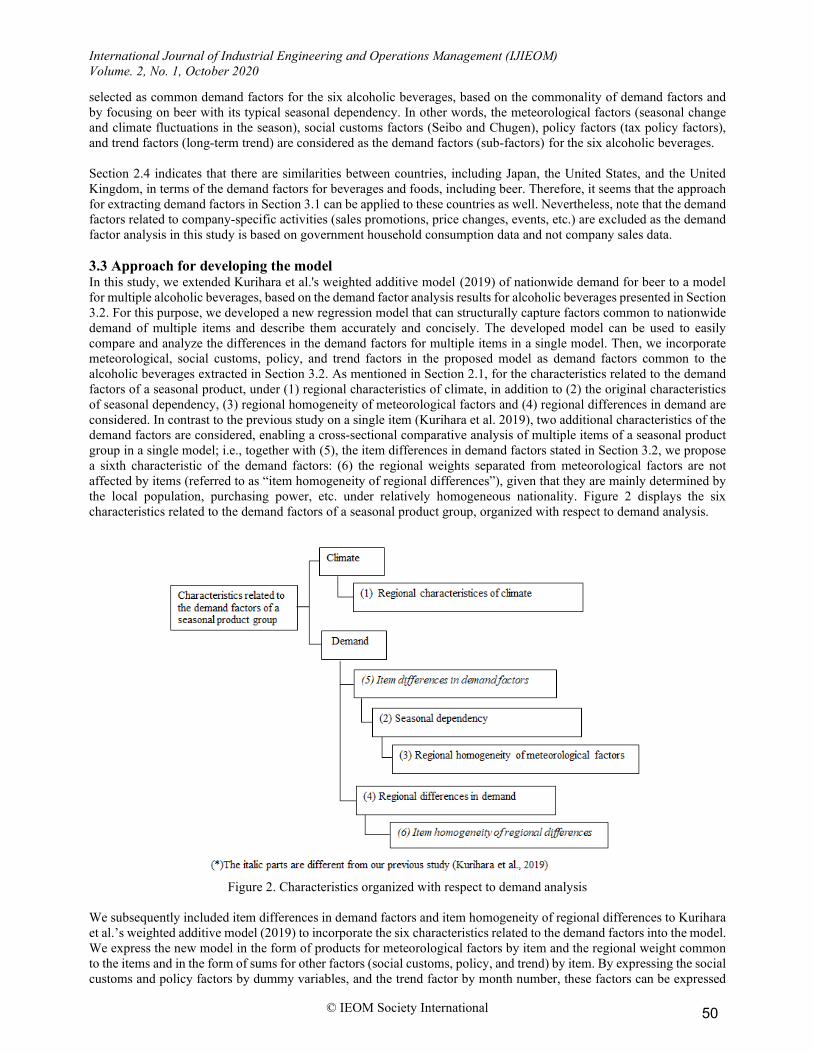
selected as common demand factors for the six alcoholic beverages, based on the commonality of demand factors and by focusing on beer with its typical seasonal dependency. In other words, the meteorological factors (seasonal change and climate fluctuations in the season), social customs factors (Seibo and Chugen), policy factors (tax policy factors), and trend factors (long-term trend) are considered as the demand factors (sub-factors) for the six alcoholic beverages. Section 2.4 indicates that there are similarities between countries, including Japan, the United States, and the United Kingdom, in terms of the demand factors for beverages and foods, including beer. Therefore, it seems that the approach for extracting demand factors in Section 3.1 can be applied to these countries as well. Nevertheless, note that the demand factors related to company-specific activities (sales promotions, price changes, events, etc.) are excluded as the demand factor analysis in this study is based on government household consumption data and not company sales data. 3.3 Approach for developing the model In this study, we extended Kurihara et al.'s weighted additive model (2019) of nationwide demand for beer to a model for multiple alcoholic beverages, based on the demand factor analysis results for alcoholic beverages presented in Section 3.2. For this purpose, we developed a new regression model that can structurally capture factors common to nationwide demand of multiple items and describe them accurately and concisely. The developed model can be used to easily compare and analyze the differences in the demand factors for multiple items in a single model. Then, we incorporate meteorological, social customs, policy, and trend factors in the proposed model as demand factors common to the alcoholic beverages extracted in Section 3.2. As mentioned in Section 2.1, for the characteristics related to the demand factors of a seasonal product, under (1) regional characteristics of climate, in addition to (2) the original characteristics of seasonal dependency, (3) regional homogeneity of meteorological factors and (4) regional differences in demand are considered. In contrast to the previous study on a single item (Kurihara et al. 2019), two additional characteristics of the demand factors are considered, enabling a cross-sectional comparative analysis of multiple items of a seasonal product group in a single model; i.e., together with (5), the item differences in demand factors stated in Section 3.2, we propose a sixth characteristic of the demand factors: (6) the regional weights separated from meteorological factors are not affected by items (referred to as “item homogeneity of regional differences”), given that they are mainly determined by the local population, purchasing power, etc. under relatively homogeneous nationality. Figure 2 displays the six characteristics related to the demand factors of a seasonal product group, organized with respect to demand analysis.

Figure 2. Characteristics organized with respect to demand analysis We subsequently included item differences in demand factors and item homogeneity of regional differences to Kurihara et al.’s weighted additive model (2019) to incorporate the six characteristics related to the demand factors into the model. We express the new model in the form of products for meteorological factors by item and the regional weight common to the items and in the form of sums for other factors (social customs, policy, and trend) by item. By expressing the social customs and policy factors by dummy variables, and the trend factor by month number, these factors can be expressed

50



in simple and general terms. Consequently, it becomes possible to concisely compare and analyze differences across multiple items in a single model by structurally capturing the characteristics of the demand factors of a seasonal product group. However, when expressed in the form of products for meteorological factors by item and regional weight, a parameter estimation problem arises in which the parameter groups become “inseparable” (Takane 1976) as they are mutually independent. To solve this problem, we develop a new algorithm using the alternating least squares method employed by Kurihara et al. (2019). This alternating least squares method was first developed by Takane et al. (1980) as a parameter estimation method for an individual difference addition model in the psychological domain. It was then applied by Yamashita (2000) to a parameter estimation of a personnel evaluation model in the personnel management domain. However, it has rarely been applied in the demand analysis domain, which is the subject of this study. 3.4 Prerequisites In this study, first, we assume the commonality of the demand factors of similar seasonal products as pointed out in Section 3.2. Second, based on our previous studies (Kurihara and Yamashita 2012; Kurihara et al. 2019), the regional climate shown in regional characteristics of climate is represented by the climate in the largest city in the region that is thought to have the greatest impact on regional demand. Third, the monthly mean air temperature and monthly total precipitation with a low correlation (0.366: September 2007 to August 2010 in Tokyo) (Kurihara and Yamashita 2012) are used as the meteorological elements to reduce the number of factors, while avoiding the problem of multicollinearity. In addition, the fluctuations in demand resulting from climate are analyzed by dividing them into stationary fluctuations (seasonal change) and nonstationary fluctuations (climate fluctuations in the season). For this purpose, the meteorological elements of demand factors are decomposed into “normal”, representing the seasonal change of a normal year, and “deviation from the normal”, representing dynamic climate fluctuations exceeding the seasonal change. Here, “normal” is the mean value over the past 30 years, and “deviation from the normal” is the difference between the actual value of the month and the normal. Fourth, based on the item homogeneity of regional differences as a seasonal product group, stated in Section 3.3, regional differences in demand shall not be affected by the item. To summarize the above, the following prerequisites are obtained: (i) All products in the same product group have common demand factors. (ii) Regional climate is represented by the climate in the largest city within that region. (iii) The normal of the monthly mean air temperature, deviation from its normal (temperature), normal of the monthly total precipitation, and deviation from its normal (precipitation) are used as the meteorological sub-factors. (iv) Regional weights that indicate regional differences in demand are common among items.

3.5 Problem formulation First, the weighted additive model of nationwide demand for beer of Kurihara et al. (2019), which serves as the basis of this study, is given as

(1) Where,

t: month number yt: nationwide household beer consumption per month at month t (yen) i: factor number (i = 1 – 4 represent meteorological sub-factors)

i = 1: normal of monthly mean air temperature (normal temperature) i = 2: deviation from normal of monthly mean air temperature (temperature deviation) i = 3: normal of monthly total precipitation (normal precipitation)

i = 4: deviation from normal of monthly total precipitation (precipitation deviation) i = 5: social customs factor 1 (Seibo: demand in December)

i = 6: social customs factor 2 (Chugen: demand in July) i = 7: tax policy factor (demand in March 2014) i = 8: trend factor (long-term trend)

ai: parameter (partial regression coefficient) a0: constant term k: region code (K: total number of region codes) wk: regional weight of region k x1tk: normal temperature in region k at month t (°C) x2tk: temperature deviation in region k at month t (°C) x3tk: normal precipitation in region k at month t (mm) x4tk: precipitation deviation in region k at month t (mm)

51



x5t: dummy variable corresponding to the demand in December (the value for December is 1; the values for the other months are 0)

x6t: dummy variable corresponding to the demand in July (the value for July is 1; the values for the other months are 0)

x7t: dummy variable corresponding to the demand in March 2014 (the value for March 2014 is 1; the values for the other years and months are 0)

x8t: month number indicating the passage of years and months (x8t = t) et: residual term

In the proposed model, it is necessary to extend Eq. (1) for a single item to an equation for multiple items by further considering item differences in demand factors and item homogeneity of regional differences. With respect to Figure 2, the regional weight wk in Eq. (1) is left as is to address the item homogeneity of regional differences. The subscript m (representing the item) is added to demand yt and demand factor ai to address item differences in demand factors. This formulates the problem as

(2) Where,

m: item number (M: total number of items to be analyzed) ymt: nationwide household consumption of item m per month at month t

ami: parameter on the factor i of item m (partial regression coefficient), am0: a constant term of item m

emt: residual term of item m Symbols other than those mentioned above are the same as in Eq. (1).

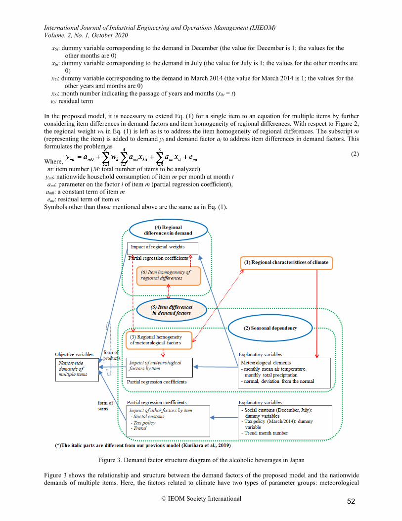
Figure 3. Demand factor structure diagram of the alcoholic beverages in Japan Figure 3 shows the relationship and structure between the demand factors of the proposed model and the nationwide demands of multiple items. Here, the factors related to climate have two types of parameter groups: meteorological

52



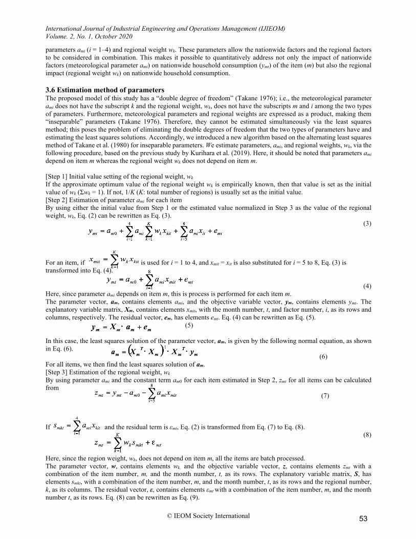
parameters ami (i = 1–4) and regional weight wk. These parameters allow the nationwide factors and the regional factors to be considered in combination. This makes it possible to quantitatively address not only the impact of nationwide factors (meteorological parameter ami) on nationwide household consumption (ymt) of the item (m) but also the regional impact (regional weight wk) on nationwide household consumption. 3.6 Estimation method of parameters The proposed model of this study has a “double degree of freedom” (Takane 1976); i.e., the meteorological parameter ami does not have the subscript k and the regional weight, wk, does not have the subscripts m and i among the two types of parameters. Furthermore, meteorological parameters and regional weights are expressed as a product, making them “inseparable” parameters (Takane 1976). Therefore, they cannot be estimated simultaneously via the least squares method; this poses the problem of eliminating the double degrees of freedom that the two types of parameters have and estimating the least squares solutions. Accordingly, we introduced a new algorithm based on the alternating least squares method of Takane et al. (1980) for inseparable parameters. We estimate parameters, ami, and regional weights, wk, via the following procedure, based on the previous study by Kurihara et al. (2019). Here, it should be noted that parameters ami depend on item m whereas the regional weight wk does not depend on item m. [Step 1] Initial value setting of the regional weight, wk If the approximate optimum value of the regional weight wk is empirically known, then that value is set as the initial value of wk (Σwk = 1). If not, 1/K (K: total number of regions) is usually set as the initial value. [Step 2] Estimation of parameter ami for each item By using either the initial value from Step 1 or the estimated value normalized in Step 3 as the value of the regional weight, wk, Eq. (2) can be rewritten as Eq. (3).

(3)

For an item, if is used for i = 1 to 4, and xmit = xit is also substituted for i = 5 to 8, Eq. (3) is transformed into Eq. (4).

(4) Here, since parameter ami depends on item m, this is process is performed for each item m. The parameter vector, am, contains elements ami, and the objective variable vector, ym, contains elements ymt. The explanatory variable matrix, Xm, contains elements xmit, with the month number, t, and factor number, i, as its rows and columns, respectively. The residual vector, em, has elements emt. Eq. (4) can be rewritten as Eq. (5). (5) In this case, the least squares solution of the parameter vector, am, is given by the following normal equation, as shown in Eq. (6).

(6) For all items, we then find the least squares solution of am. [Step 3] Estimation of the regional weight, wk By using parameter ami and the constant term am0 for each item estimated in Step 2, zmt for all items can be calculated from

(7) If and the residual term is εmt, Eq. (2) is transformed from Eq. (7) to Eq. (8).

(8) Here, since the region weight, wk, does not depend on item m, all the items are batch processed. The parameter vector, w, contains elements wk, and the objective variable vector, z, contains elements zmt with a combination of the item number, m, and the month number, t, as its rows. The explanatory variable matrix, S, has elements smkt, with a combination of the item number, m, and the month number, t, as its rows and the regional number, k, as its columns. The residual vector, ε, contains elements εmt with a combination of the item number, m, and the month number t, as its rows. Eq. (8) can be rewritten as Eq. (9).

53



(9) In this case, the least squares solution for parameter vector w is given by the normal equation shown in Eq. (10).

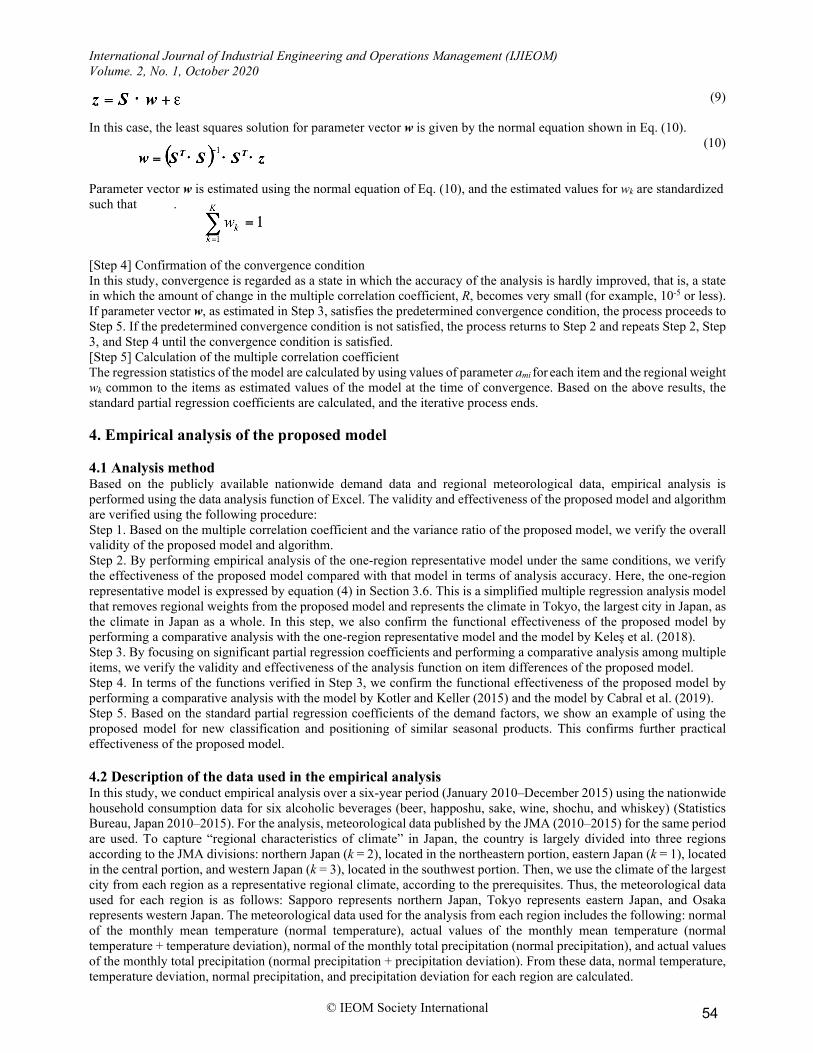
(10) Parameter vector w is estimated using the normal equation of Eq. (10), and the estimated values for wk are standardized such that . [Step 4] Confirmation of the convergence condition In this study, convergence is regarded as a state in which the accuracy of the analysis is hardly improved, that is, a state in which the amount of change in the multiple correlation coefficient, R, becomes very small (for example, 10-5 or less). If parameter vector w, as estimated in Step 3, satisfies the predetermined convergence condition, the process proceeds to Step 5. If the predetermined convergence condition is not satisfied, the process returns to Step 2 and repeats Step 2, Step 3, and Step 4 until the convergence condition is satisfied. [Step 5] Calculation of the multiple correlation coefficient The regression statistics of the model are calculated by using values of parameter ami for each item and the regional weight wk common to the items as estimated values of the model at the time of convergence. Based on the above results, the standard partial regression coefficients are calculated, and the iterative process ends. 4. Empirical analysis of the proposed model 4.1 Analysis method Based on the publicly available nationwide demand data and regional meteorological data, empirical analysis is performed using the data analysis function of Excel. The validity and effectiveness of the proposed model and algorithm are verified using the following procedure: Step 1. Based on the multiple correlation coefficient and the variance ratio of the proposed model, we verify the overall validity of the proposed model and algorithm. Step 2. By performing empirical analysis of the one-region representative model under the same conditions, we verify the effectiveness of the proposed model compared with that model in terms of analysis accuracy. Here, the one-region representative model is expressed by equation (4) in Section 3.6. This is a simplified multiple regression analysis model that removes regional weights from the proposed model and represents the climate in Tokyo, the largest city in Japan, as the climate in Japan as a whole. In this step, we also confirm the functional effectiveness of the proposed model by performing a comparative analysis with the one-region representative model and the model by Keleş et al. (2018). Step 3. By focusing on significant partial regression coefficients and performing a comparative analysis among multiple items, we verify the validity and effectiveness of the analysis function on item differences of the proposed model. Step 4. In terms of the functions verified in Step 3, we confirm the functional effectiveness of the proposed model by performing a comparative analysis with the model by Kotler and Keller (2015) and the model by Cabral et al. (2019). Step 5. Based on the standard partial regression coefficients of the demand factors, we show an example of using the proposed model for new classification and positioning of similar seasonal products. This confirms further practical effectiveness of the proposed model. 4.2 Description of the data used in the empirical analysis In this study, we conduct empirical analysis over a six-year period (January 2010–December 2015) using the nationwide household consumption data for six alcoholic beverages (beer, happoshu, sake, wine, shochu, and whiskey) (Statistics Bureau, Japan 2010–2015). For the analysis, meteorological data published by the JMA (2010–2015) for the same period are used. To capture “regional characteristics of climate” in Japan, the country is largely divided into three regions according to the JMA divisions: northern Japan (k = 2), located in the northeastern portion, eastern Japan (k = 1), located in the central portion, and western Japan (k = 3), located in the southwest portion. Then, we use the climate of the largest city from each region as a representative regional climate, according to the prerequisites. Thus, the meteorological data used for each region is as follows: Sapporo represents northern Japan, Tokyo represents eastern Japan, and Osaka represents western Japan. The meteorological data used for the analysis from each region includes the following: normal of the monthly mean temperature (normal temperature), actual values of the monthly mean temperature (normal temperature + temperature deviation), normal of the monthly total precipitation (normal precipitation), and actual values of the monthly total precipitation (normal precipitation + precipitation deviation). From these data, normal temperature, temperature deviation, normal precipitation, and precipitation deviation for each region are calculated.

54



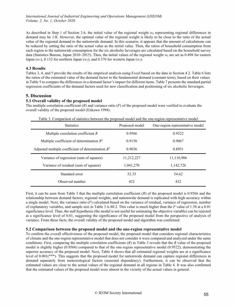
As described in Step 1 of Section 3.6, the initial value of the regional weight wk representing regional differences in demand may be 1/K. However, the optimal value of the regional weight is likely to be close to the ratio of the actual value of the regional demand to the nationwide demand. In this scenario, it appears that the amount of calculations can be reduced by setting the ratio of the actual value as the initial value. Then, the ratios of household consumption from each region to the nationwide consumption for the six alcoholic beverages are calculated based on the household survey data (Statistics Bureau, Japan 2010–2015). Thus, the initial values of the regional weight wk are set as 0.498 for eastern Japan (w1), 0.132 for northern Japan (w2), and 0.370 for western Japan (w3). 4.3 Results Tables 3, 4, and 5 provide the results of the empirical analysis using Excel based on the data in Section 4.2. Table 6 lists the ratios of the estimated value of the demand factor to the fundamental demand (constant term), based on their values in Table 5 to compare the differences in a demand factor’s impact for different items. Table 7 presents the standard partial regression coefficients of the demand factors used for new classification and positioning of six alcoholic beverages. 5. Discussion 5.1 Overall validity of the proposed model The multiple correlation coefficient (R) and variance ratio (F) of the proposed model were verified to evaluate the overall validity of the proposed model (Enkawa 1994).

Table 3. Comparison of statistics between the proposed model and the one-region representative model

Statistics

Proposed model One-region representative model

Multiple correlation coefficient R 0.9566 0.9522

Multiple coefficient of determination R2 0.9150 0.9067

Adjusted multiple coefficient of determination R2 0.9036 0.8951

Variance of regression (sum of squares) 11,212,227 11,110,906

Variance of residual (sum of squares) 1,041,270 1,142,726

Standard error 52.35 54.62

Observed number 432 432

First, it can be seen from Table 3 that the multiple correlation coefficient (R) of the proposed model is 0.9566 and the relationship between demand factors, regional weights, and nationwide demand is replicated with high accuracy within a single model. Next, the variance ratio (F) calculated based on the variance of residual, variance of regression, number of explanatory variables, and sample size in Table 3 is 80.2. This value is much higher than the F value of 1.58 at a 0.01 significance level. Thus, the null hypothesis (the model is not useful for estimating the objective variable) can be rejected at a significance level of 0.01, suggesting the significance of the proposed model from the perspective of analysis of variance. From these facts, the overall validity of the proposed model and algorithm was confirmed. 5.2 Comparison between the proposed model and the one-region representative model To confirm the overall effectiveness of the proposed model, the proposed model that considers regional characteristics of climate and the one-region representative model that does not consider it were compared and analyzed under the same conditions. First, comparing the multiple correlation coefficients (R) in Table 3 reveals that the R value of the proposed model is slightly higher (0.9566) compared to that of the one-region representative model (0.9522), demonstrating the superior accuracy of the proposed model. Next, Table 4 shows that all estimated regional weights are at a significance level of 0.001(***). This suggests that the proposed model for nationwide demand can capture regional differences in demand separately from meteorological factors (seasonal dependency). Furthermore, it can be observed that the estimated values are close to the actual values of the regional demand in all regions in Table 4. It was also confirmed that the estimated values of the proposed model were almost in the vicinity of the actual values in general.

55



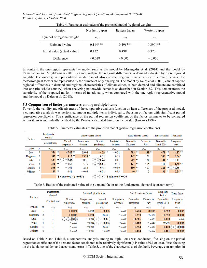
Table 4. Parameter estimates of the proposed model (regional weight)

Region Northern Japan Eastern Japan Western Japan

Symbol of regional weight w2 w1 w3

Estimated value 0.114*** 0.496*** 0.390***

Initial value (actual value) 0.132 0.498 0.370

Difference - 0.018 - 0.002 + 0.020

In contrast, the one-region representative model such as the model by Mirasgedis et al. (2014) and the model by Ramanathan and Muyldermans (2010), cannot analyze the regional differences in demand indicated by these regional weights. The one-region representative model cannot also consider regional characteristics of climate because the meteorological factors are represented by the climate of only one region. The model by Keleş et al. (2018) cannot capture regional differences in demand and regional characteristics of climate either, as both demand and climate are combined into one (the whole country) when analyzing nationwide demand; as described in Section 2.2. This demonstrates the superiority of the proposed model in terms of functionality when compared with the one-region representative model and the model by Keleş et al. (2018). 5.3 Comparison of factor parameters among multiple items To verify the validity and effectiveness of the comparative analysis function on item differences of the proposed model, a comparative analysis was performed among multiple items individually, focusing on factors with significant partial regression coefficients. The significance of the partial regression coefficient of the factor parameter to be compared across items is individually verified by the P-value calculated based on the t-value (Enkawa 1994).

Table 5. Parameter estimates of the proposed model (partial regression coefficient)

Table 6. Ratios of the estimated value of the demand factor to the fundamental demand (constant term)

Based on Table 5 and Table 6, a comparative analysis among multiple items was conducted, focusing on the partial regression coefficient of the demand factor considered to be relatively significant (a P-value of 0.1 or less). First, focusing on the fundamental demand (a constant term) in Table 5, one of the characteristics of alcoholic beverage consumption in

56



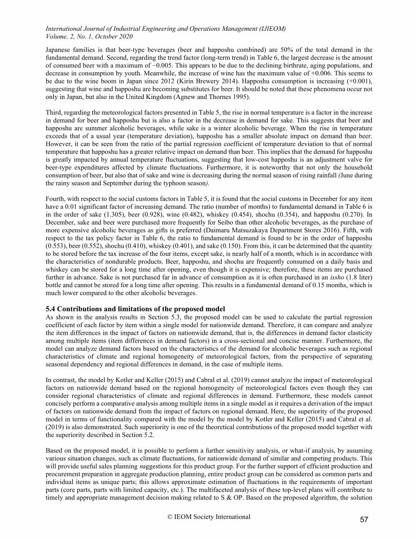
Japanese families is that beer-type beverages (beer and happoshu combined) are 50% of the total demand in the fundamental demand. Second, regarding the trend factor (long-term trend) in Table 6, the largest decrease is the amount of consumed beer with a maximum of −0.005. This appears to be due to the declining birthrate, aging populations, and decrease in consumption by youth. Meanwhile, the increase of wine has the maximum value of +0.006. This seems to be due to the wine boom in Japan since 2012 (Kirin Brewery 2014). Happoshu consumption is increasing (+0.001), suggesting that wine and happoshu are becoming substitutes for beer. It should be noted that these phenomena occur not only in Japan, but also in the United Kingdom (Agnew and Thornes 1995). Third, regarding the meteorological factors presented in Table 5, the rise in normal temperature is a factor in the increase in demand for beer and happoshu but is also a factor in the decrease in demand for sake. This suggests that beer and happoshu are summer alcoholic beverages, while sake is a winter alcoholic beverage. When the rise in temperature exceeds that of a usual year (temperature deviation), happoshu has a smaller absolute impact on demand than beer. However, it can be seen from the ratio of the partial regression coefficient of temperature deviation to that of normal temperature that happoshu has a greater relative impact on demand than beer. This implies that the demand for happoshu is greatly impacted by annual temperature fluctuations, suggesting that low-cost happoshu is an adjustment valve for beer-type expenditures affected by climate fluctuations. Furthermore, it is noteworthy that not only the household consumption of beer, but also that of sake and wine is decreasing during the normal season of rising rainfall (June during the rainy season and September during the typhoon season). Fourth, with respect to the social customs factors in Table 5, it is found that the social customs in December for any item have a 0.01 significant factor of increasing demand. The ratio (number of months) to fundamental demand in Table 6 is in the order of sake (1.305), beer (0.928), wine (0.482), whiskey (0.454), shochu (0.354), and happoshu (0.270). In December, sake and beer were purchased more frequently for Seibo than other alcoholic beverages, as the purchase of more expensive alcoholic beverages as gifts is preferred (Daimaru Matsuzakaya Department Stores 2016). Fifth, with respect to the tax policy factor in Table 6, the ratio to fundamental demand is found to be in the order of happoshu (0.553), beer (0.552), shochu (0.410), whiskey (0.401), and sake (0.150). From this, it can be determined that the quantity to be stored before the tax increase of the four items, except sake, is nearly half of a month, which is in accordance with the characteristics of nondurable products. Beer, happoshu, and shochu are frequently consumed on a daily basis and whiskey can be stored for a long time after opening, even though it is expensive; therefore, these items are purchased further in advance. Sake is not purchased far in advance of consumption as it is often purchased in an issho (1.8 liter) bottle and cannot be stored for a long time after opening. This results in a fundamental demand of 0.15 months, which is much lower compared to the other alcoholic beverages. 5.4 Contributions and limitations of the proposed model As shown in the analysis results in Section 5.3, the proposed model can be used to calculate the partial regression coefficient of each factor by item within a single model for nationwide demand. Therefore, it can compare and analyze the item differences in the impact of factors on nationwide demand, that is, the differences in demand factor elasticity among multiple items (item differences in demand factors) in a cross-sectional and concise manner. Furthermore, the model can analyze demand factors based on the characteristics of the demand for alcoholic beverages such as regional characteristics of climate and regional homogeneity of meteorological factors, from the perspective of separating seasonal dependency and regional differences in demand, in the case of multiple items. In contrast, the model by Kotler and Keller (2015) and Cabral et al. (2019) cannot analyze the impact of meteorological factors on nationwide demand based on the regional homogeneity of meteorological factors even though they can consider regional characteristics of climate and regional differences in demand. Furthermore, these models cannot concisely perform a comparative analysis among multiple items in a single model as it requires a derivation of the impact of factors on nationwide demand from the impact of factors on regional demand. Here, the superiority of the proposed model in terms of functionality compared with the model by the model by Kotler and Keller (2015) and Cabral et al. (2019) is also demonstrated. Such superiority is one of the theoretical contributions of the proposed model together with the superiority described in Section 5.2. Based on the proposed model, it is possible to perform a further sensitivity analysis, or what-if analysis, by assuming various situation changes, such as climate fluctuations, for nationwide demand of similar and competing products. This will provide useful sales planning suggestions for this product group. For the further support of efficient production and procurement preparation in aggregate production planning, entire product group can be considered as common parts and individual items as unique parts; this allows approximate estimation of fluctuations in the requirements of important parts (core parts, parts with limited capacity, etc.). The multifaceted analysis of these top-level plans will contribute to timely and appropriate management decision making related to S & OP. Based on the proposed algorithm, the solution

57



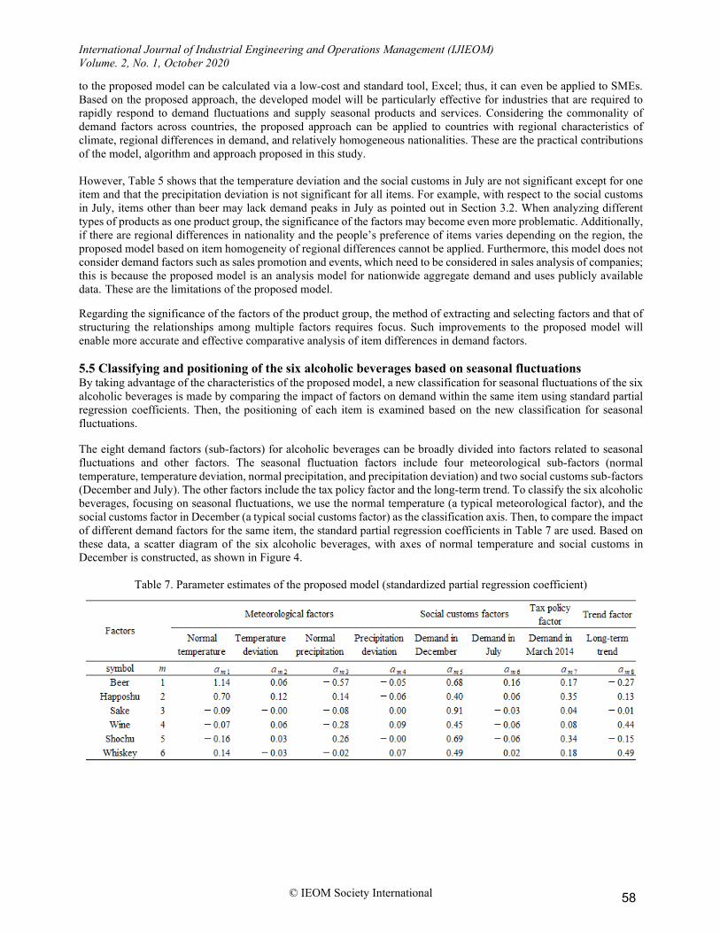
to the proposed model can be calculated via a low-cost and standard tool, Excel; thus, it can even be applied to SMEs. Based on the proposed approach, the developed model will be particularly effective for industries that are required to rapidly respond to demand fluctuations and supply seasonal products and services. Considering the commonality of demand factors across countries, the proposed approach can be applied to countries with regional characteristics of climate, regional differences in demand, and relatively homogeneous nationalities. These are the practical contributions of the model, algorithm and approach proposed in this study. However, Table 5 shows that the temperature deviation and the social customs in July are not significant except for one item and that the precipitation deviation is not significant for all items. For example, with respect to the social customs in July, items other than beer may lack demand peaks in July as pointed out in Section 3.2. When analyzing different types of products as one product group, the significance of the factors may become even more problematic. Additionally, if there are regional differences in nationality and the people’s preference of items varies depending on the region, the proposed model based on item homogeneity of regional differences cannot be applied. Furthermore, this model does not consider demand factors such as sales promotion and events, which need to be considered in sales analysis of companies; this is because the proposed model is an analysis model for nationwide aggregate demand and uses publicly available data. These are the limitations of the proposed model. Regarding the significance of the factors of the product group, the method of extracting and selecting factors and that of structuring the relationships among multiple factors requires focus. Such improvements to the proposed model will enable more accurate and effective comparative analysis of item differences in demand factors. 5.5 Classifying and positioning of the six alcoholic beverages based on seasonal fluctuations By taking advantage of the characteristics of the proposed model, a new classification for seasonal fluctuations of the six alcoholic beverages is made by comparing the impact of factors on demand within the same item using standard partial regression coefficients. Then, the positioning of each item is examined based on the new classification for seasonal fluctuations. The eight demand factors (sub-factors) for alcoholic beverages can be broadly divided into factors related to seasonal fluctuations and other factors. The seasonal fluctuation factors include four meteorological sub-factors (normal temperature, temperature deviation, normal precipitation, and precipitation deviation) and two social customs sub-factors (December and July). The other factors include the tax policy factor and the long-term trend. To classify the six alcoholic beverages, focusing on seasonal fluctuations, we use the normal temperature (a typical meteorological factor), and the social customs factor in December (a typical social customs factor) as the classification axis. Then, to compare the impact of different demand factors for the same item, the standard partial regression coefficients in Table 7 are used. Based on these data, a scatter diagram of the six alcoholic beverages, with axes of normal temperature and social customs in December is constructed, as shown in Figure 4.

Table 7. Parameter estimates of the proposed model (standardized partial regression coefficient)

58



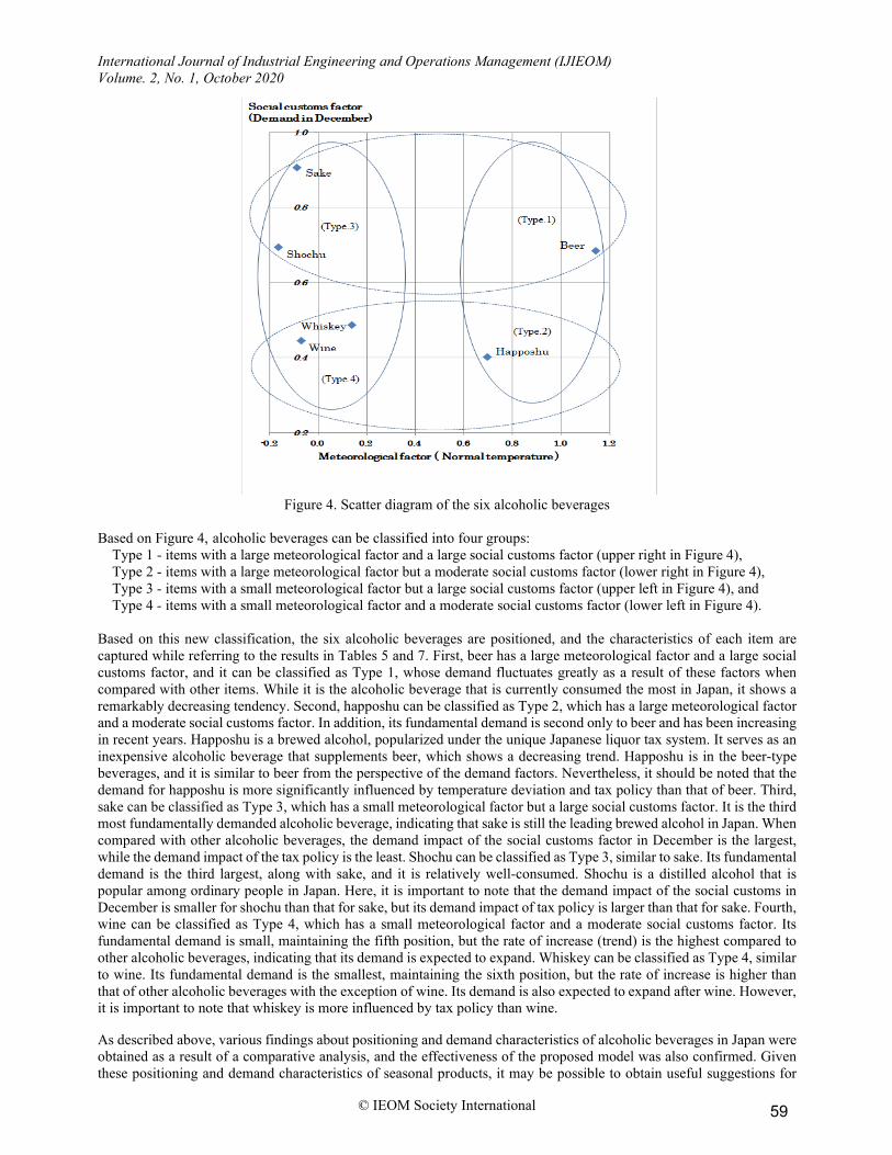
Figure 4. Scatter diagram of the six alcoholic beverages

Based on Figure 4, alcoholic beverages can be classified into four groups:

Type 1 - items with a large meteorological factor and a large social customs factor (upper right in Figure 4), Type 2 - items with a large meteorological factor but a moderate social customs factor (lower right in Figure 4), Type 3 - items with a small meteorological factor but a large social customs factor (upper left in Figure 4), and Type 4 - items with a small meteorological factor and a moderate social customs factor (lower left in Figure 4).

Based on this new classification, the six alcoholic beverages are positioned, and the characteristics of each item are captured while referring to the results in Tables 5 and 7. First, beer has a large meteorological factor and a large social customs factor, and it can be classified as Type 1, whose demand fluctuates greatly as a result of these factors when compared with other items. While it is the alcoholic beverage that is currently consumed the most in Japan, it shows a remarkably decreasing tendency. Second, happoshu can be classified as Type 2, which has a large meteorological factor and a moderate social customs factor. In addition, its fundamental demand is second only to beer and has been increasing in recent years. Happoshu is a brewed alcohol, popularized under the unique Japanese liquor tax system. It serves as an inexpensive alcoholic beverage that supplements beer, which shows a decreasing trend. Happoshu is in the beer-type beverages, and it is similar to beer from the perspective of the demand factors. Nevertheless, it should be noted that the demand for happoshu is more significantly influenced by temperature deviation and tax policy than that of beer. Third, sake can be classified as Type 3, which has a small meteorological factor but a large social customs factor. It is the third most fundamentally demanded alcoholic beverage, indicating that sake is still the leading brewed alcohol in Japan. When compared with other alcoholic beverages, the demand impact of the social customs factor in December is the largest, while the demand impact of the tax policy is the least. Shochu can be classified as Type 3, similar to sake. Its fundamental demand is the third largest, along with sake, and it is relatively well-consumed. Shochu is a distilled alcohol that is popular among ordinary people in Japan. Here, it is important to note that the demand impact of the social customs in December is smaller for shochu than that for sake, but its demand impact of tax policy is larger than that for sake. Fourth, wine can be classified as Type 4, which has a small meteorological factor and a moderate social customs factor. Its fundamental demand is small, maintaining the fifth position, but the rate of increase (trend) is the highest compared to other alcoholic beverages, indicating that its demand is expected to expand. Whiskey can be classified as Type 4, similar to wine. Its fundamental demand is the smallest, maintaining the sixth position, but the rate of increase is higher than that of other alcoholic beverages with the exception of wine. Its demand is also expected to expand after wine. However, it is important to note that whiskey is more influenced by tax policy than wine. As described above, various findings about positioning and demand characteristics of alcoholic beverages in Japan were obtained as a result of a comparative analysis, and the effectiveness of the proposed model was also confirmed. Given these positioning and demand characteristics of seasonal products, it may be possible to obtain useful suggestions for

59



appropriate sales policies and plans within a group of similar and competing seasonal products, according to the season and time. This is also one of the practical contributions of the proposed model. 6. Conclusion In this study, we first extracted six characteristics related to the demand factors for Japanese alcoholic beverages as a group of similar seasonal products, i.e., “regional characteristics of climate”, “seasonal dependency”, “regional homogeneity of meteorological factors”, “regional differences in demand”, “item differences in demand factors”, and “item homogeneity of regional differences”. Next, based on the extracted characteristics, we proposed a new item-difference comparative analysis model on the nationwide demand for alcoholic beverages by extending the weighted additive model for a single item (Kurihara et al. 2019) to that for multiple items. The proposed model is expressed as the product of mutually independent meteorological factors by item and regional weights. This enables a comparative analysis of demand factors in the form of separating the meteorological factors and the regional weights, in the case of multiple items. However, this creates a new problem of estimating inseparable parameters. To solve this problem, we proposed a new algorithm based on the alternating least squares method developed in the field of psychology. We conducted empirical analysis of the proposed model based on publicly available data for six alcoholic beverages consumed in Japan (beer, happoshu, sake, shochu, wine, and whiskey). Based on the results, we confirmed the validity of the model, algorithm and approach proposed in this study. The main theoretical contributions of this study are as follows. The proposed model makes it possible to easily and cross-sectionally analyze item differences in demand factors (including seasonal dependency) and regional differences in demand within one model, from the perspective of separating seasonal dependency and regional differences in demand. Compared with the one-region representative model, the proposed model is more accurate and allows the regional differences in demand to be analyzed, while considering the regional characteristics of climate. Moreover, compared with the regional demand accumulation model, the proposed model enables cross-sectional and concise analysis of item differences in demand factors within one model, while considering the regional homogeneity of meteorological factors. The main practical contributions of this study are as follows. First, a sensitivity analysis to situation changes based on the proposed model can provide useful suggestions in sales planning for a group of similar competing products. A rough requirement estimation based on the proposed model can support efficient production and procurement preparation for the entire product group in aggregate production planning. Through these things, the proposed model can contribute to timely and appropriate management decision making related to S & OP. Furthermore, various findings obtained through new classification via the model will be effective for sales policies. Second, based on the proposed algorithm, the solution of the model can be easily and cheaply calculated using the standard tool Excel; thus, the proposed model will be applicable to SMEs. Third, given the commonality of demand factors across countries, the proposed approach can be applied to industries that supply seasonal products following demand fluctuations in countries with regional characteristics of climate and relatively homogeneous nationalities. However, there are some demand factors (such as the social customs in July) in the proposed model that are not significant for items other than beer as we focused on beer in this study and extracted factors to build the model. This is more conspicuous when targeting different types of products. Additionally, the model in this study cannot be applied when the nationality differs by region and the people’s item preferences vary by region; this is because the model presupposes item homogeneity of regional differences. Furthermore, the demand factors (such as sales promotion and events) that should be considered in a company’s sales analysis are excluded in the proposed model. This is because the model is an analysis model for nationwide demand, based on publicly available data. These should be considered to be the limitations of the proposed model in this study. Following this study, we will aim to develop a demand analysis model that can analyze item differences within a seasonal product group more accurately and effectively by increasing the number of significant factors for items other than beer. For this purpose, we will focus on the methods of extracting and selecting factors and structuring the relationship among factors. In the future, we will pursue a study on a new demand forecasting model that is based on meteorological forecast data, rather than actual meteorological data. References Agnew, M., and Thornes, J., The weather sensitivity of the UK food retail and distribution industry, Meteorological

Applications, vol.2, no.2, pp.137-147, 1995. Apadula, F., Bassini, A., and Scapin, S., Relationship between meteorological variables and monthly electricity demand,

Applied Energy, vol.98, pp.346-356, 2012.

60



Arunraj, N. S., and Ahrens, D., A hybrid seasonal autoregressive integrated moving average and quantile regression for daily food sales forecasting, International Journal of Production Economics, vol.170, pp.321-335, 2015.

Barbosa, N. P., Christo, E. S., and Costa, K. A., Demand forecasting for production planning in a food company, ARPN Journal of Engineering and Applied Sciences, vol.10, no.16, pp.7137-7141, 2015.

Beer Industry Electronic Commerce Coalition (BIECC), Hitting the Mark: Accuracy in Beer Sales Forecasting, BIECC, Alexandria, 2009.

Bowersox, D.J., Closs, D.J., and Cooper, M.B., Supply Chain Logistics Management, 3rd Edition, McGraw-Hill, New York, 2010.

Bratina, D., and Faganel, A., Forecasting the primary demand for a beer brand using time series analysis, Organizacija, vol.41, no.3, pp.116-123, 2008.

Cabral, M., Loureiro, D., Amado, C., Mamade, A., and Covas, D., Demand scenario planning approach using regression techniques and application to network sectors in Portugal, Water Policy, vol.21, pp.394-411, 2019.

Daimaru Matsuzakaya Department Stores, Chugen to Seibo no Chigai (Difference between a midyear gift called Chugen and a year-end gift called Seibo) (2016), http:// www.matsuzakaya.co.jp/ochugen_chisiki/oseibo.html/, March 31, 2017.

Enkawa, T., Multivariate analysis, in Japan Industrial Management Association (eds.), Industrial Management Handbook, Maruzen, Tokyo, 1994.

Fogarty, J., The demand for beer, wine and spirits: A survey of the literature, Journal of Economic Surveys, vol.24, no.3, pp.428-478, 2010.

Honda, M., Keiei no tameno jyuyo no bunseki to yosoku (Demand analysis and forecast for management), SANNO Institute of management Publication Dept., Tokyo, 2000.

Japan Meteorological Agency, News Release (2010), https://ds.data.jma.go.jp/tcc/tcc/news/press 20100910.pdf, September 30, 2016.

Japan Meteorological Agency, News Release (2012), https://www.jma.go.jp/jma/press/1203/01c/tenko121202.html, September 30, 2016.

Japan Meteorological Agency, Table of Monthly Climate Statistics (2010–2015), http://www.data.jma.go.jp/obd/ stats/data/en/, March 31, 2017.

Keleş, B., Gómez-Acevedo, P., and Shaikh, N. I., The impact of systematic changes in weather on the supply and demand of beverages, International Journal of Production Economics, vol.195, pp.186-197, 2018.

Kirin Brewery, News Release (2014), https:// www.kirin.co.jp/company/news/2014/0903_02.html, Octorber 7, 2017. Kotler, P. and Keller, K. L., Marketing Management, 15th Edition, Pearson, Harlow, 2015. Kurihara, T., and Yamashita, H., A weighted additive model of regional factors for demand forecast of air-conditioners:

using meteorological data, Journal of Japan Association for Management Systems, vol.29, no.1, pp. 43-48, 2012. Kurihara, T., Kawanaka, T., and Yamashita, H., A butterfly catastrophe model of seasonal products on characteristics of

production and inventory management, considering product price, Journal of Japan Association for Management Systems, vol.35, no.1, pp.1-8, 2018.

Kurihara, T., Kawanaka, T., and Yamashita, H., A weighted additive model for the whole demand analysis of a seasonally dependent product using meteorological and regional data, considering social customs factors and policy factors: Focus on Japanese beer demand structure, Industrial Engineering and Management Systems, vol.18, no.4, pp.761-775, 2019.

Kuroda, M., Production Planning Method, in Japan Industrial Management Association (eds.), Industrial Management Handbook, Maruzen, Tokyo, 1994.

Lenten, L.J.A., and Moosa, I.A., Modelling the trend and seasonality in the consumption of alcoholic beverages in the United Kingdom, Applied Economics, vol.31, pp.795-804, 1999.

Makridakis, S., Wheelwright, S., Hyndman, R., and Chang, Y., Forecasting Methods and Applications, 3rd Edition, John Wiley & Sons, New York, 1998.

Mirasgedis, S., Georgopoulou, E., Sarafidis, Y., Papagiannaki, K., and Lalas, D.P., The impact of climate change on the pattern of demand for bottled water and non-alcoholic beverages, Business Strategy and the Environment, vol.23, no.4, pp.272-288, 2014.

Mircetic, D., Nikolicic, S., Maslaric, M., Ralevic, N., and Debelic, B., Development of S-ARIMA model for forecasting demand in a beverage supply chain, Open Engineering, vol.6, no.1, pp.407-411, 2016.

Moosa, I. A., and Baxter, J.L., Modelling the trend and seasonals within an AIDS model of the demand for alcoholic beverages in the United Kingdom, Applied Economics, vol.17, pp.95-106, 2002.

Nakatani, Y., Nihon no katei ni okeru biru jyuyo (Beer demand in Japanese family), Journal of Japan Business Management Association, vol.2, pp.13-19, 2012.

National Research Institute of Brewing, Umai sakeno kagaku (Science of delicious liquor), SB Creative, Tokyo, 2007. Ramanathan, U., and Muyldermans, L., Identifying demand factors for promotional planning and forecasting: a case of

a soft drink company in the UK, International Journal of Production Economics, vol.128, pp.538-545, 2010.

61



Sanders, N.R., Forecasting Guidelines and Methods, in P. M. Swamidass (ed.), Encyclopedia of Production and Manufacturing Management, Kluwer Academic Publishers, Norwell, 2000.

Statics Bureau of Japan, Family Income and Expenditure Survey (2010–2015), https://www.stat.go.jp/english/data/ kakei/1561.html, March.3, 2017.

Takane.Y., Shinri-gaku ni okeru Hi-keiryou Deta no Kaiseki (Nonmetric Data Analysis in Psychology), The University of Tokyo, Ph.D. in thesis, 1976.

Takane,Y., Young,F.W., and de Leeuw, J., An individual differences additive model: an alternating least squares method with optical scaling features, Psychometrica, Vol.45, pp.183-209, 1980.

Tirkes, G., Guray, C., and Celebi, N., Demand forecasting: a comparison between the holt-winters, trend analysis and decomposition model, Technical Gazette, Suppl. 2, pp.503-509, 2017.

Veiga, C. P., Veiga, C. R., Catapan, A., Tortato, U., and Silva, W. V., Demand forecasting in food retail: a comparison between the holt-winters and ARIMA model, WSEAS Transactions on Business and Economics, vol.11, pp.608-614, 2014.

Yamashita, H., Jinji-jyoho kanri no tame no Hyotei-keikou Bunseki Model (A rating trend analysis model for personnel information management), Keirin-shobo, Tokyo, 2000.

Biographies Tsuyoshi Kurihara is a certified and accredited meteorologist of Japan. He earned Bachelor Degree of Engineering in Faculty of Engineering from Tokyo Institute of Technology, Japan, Master Degree of Commerce in Master course Graduate school of Commerce from Meiji University. He had worked as a system engineer in production management and a subleader of the supply chain innovation project at Mazda Motor Cooperation. His research interests include Industrial Management, Management Modeling, and Supply Chain Management. He is member of Japan Association for Management Systems and Meteorological Society of Japan. Takaaki Kawanaka is currently a lecturer in Institute for Innovation in International Engineering Education, Graduate School of Engineering, the University of Tokyo, Japan. He earned Bachelor Degree of Engineering in Faculty of Science and Engineering from Waseda University, Japan, Master Degree of Engineering in Master course Graduate school of Science and Engineering from Waseda University and Doctor Degree of Engineering in Doctor course Graduate school of Engineering from the University of Tokyo, Japan. His research interests are mainly focused on Industrial Engineering, Management Modeling and Information Security Management. He is member of Japan Association for Management Systems, Japan Industrial Management Association, Japan Society of Security Management, and Information Processing Society of Japan. Hiroshi Yamashita is currently Professor in Department of Commerce, Meiji University, Japan. He earned Bachelor Degree of Engineering in Faculty of Science and Engineering from Waseda University, Japan, Master Degree of Engineering in Master course Graduate school of Science and Engineering from Waseda University, Doctor Degree of Engineering in Doctor course Graduate school of Science and Engineering from Waseda University and Doctor of Commerce from Meiji University. His research interests are mainly focused on Human Resource Management, Management Quality Science and Management Modeling. He is member of Japan Association for Management Systems, Japan Association for Communication, Information and

62

Documents

A Weighted Additive Model for Comparative Analysis on