Embed Size (px)
Citation preview
A wavelet approach of investing behaviors and their effects on risk exposuresRoman Mestre*
IntroductionMarkowitz (1952) Modern Portfolio Theory led the development of the Capital Asset Pricing Model (CAPM) which was created by Sharpe (1964), Lintner (1965) and Mossin (1966). Its mathematical equation, the Securities Market Line (SML), is similar to a sim-ple regression model between the asset risk premium and the risks of the Market. This is also known as the Market Model. According to the CAPM hypothesis, the market is the only source of risk and the agents have homogeneous investing behavior. Systematic risk is measured through estimations of the traditional Market Model. Many authors such as Black et al. (1972) and then Fama and MacBeth (1973) highlighted several statisti-cal anomalies in the model, more particularly, the non-robustness of the methods used
Abstract
Exposure to market risk is a core objective of the Capital Asset Pricing Model (CAPM) with a focus on systematic risk. However, traditional OLS Beta model estimations (Ordinary Least Squares) are plagued with several statistical issues. Moreover, the CAPM considers only one source of risk and supposes that investors only engage in similar behaviors. In order to analyze short and long exposures to different sources of risk, we developed a Time–Frequency Multi-Betas Model with ARMA-EGARCH errors (Auto Regressive Moving Average Exponential AutoRegressive Conditional Heteroske-dasticity). Our model considers gold, oil, and Fama–French factors as supplementary sources of risk and wavelets decompositions. We used 30 French stocks listed on the CAC40 (Cotations Assistées Continues 40) within a daily period from 2005 to 2015. The conjugation of the wavelet decompositions and the parameters estimates constitutes decision-making support for managers by multiplying the interpretive possibilities. In the short-run, (“Noise Trader” and “High-Frequency Trader”) only a few equities are insensitive to Oil and Gold fluctuations, and the estimated Market Betas parameters are scant different compared to the Model without wavelets. Oppositely, in the long-run, (fundamentalists investors), Oil and Gold affect all stocks but their impact varies accord-ing to the Beta (sensitivity to the market). We also observed significant differences between parameters estimated with and without wavelets.
Keywords: Risk exposures, CAPM, Multi-betas model, Time–frequency analysis, MODWT, Oil, Gold
JEL Classification: C32, C58, C65, G11, G40
Open Access
© The Author(s) 2021. Open Access This article is licensed under a Creative Commons Attribution 4.0 International License, which permits use, sharing, adaptation, distribution and reproduction in any medium or format, as long as you give appropriate credit to the original author(s) and the source, provide a link to the Creative Commons licence, and indicate if changes were made. The images or other third party material in this article are included in the article’s Creative Commons licence, unless indicated otherwise in a credit line to the mate-rial. If material is not included in the article’s Creative Commons licence and your intended use is not permitted by statutory regulation or exceeds the permitted use, you will need to obtain permission directly from the copyright holder. To view a copy of this licence, visit http:// creat iveco mmons. org/ licen ses/ by/4. 0/.
RESEARCH
Mestre Financ Innov (2021) 7:24 https://doi.org/10.1186/s40854-021-00239-z Financial Innovation
*Correspondence: [email protected] MRE Université de Montpellier, UFR d’économie Avenue Raymond Dugrand– Site de Richter C.S. 79606, 34960 Montpellier Cedex 2, France

Page 2 of 37Mestre Financ Innov (2021) 7:24
resulting from the autocorrelation-heteroscedasticity in the residuals of the estimations, and the potential absence of exogenous variables in the model.
Following the first tests of CAPM, Fabozzi and Francis (1978) indicated that the Beta parameter is unstable over time, resulting in confirmation by Bos and Newbold (1984). This characteristic of Beta implies that time-varying parameter estimation is required. Many methods have been tested such as rolling-window, recursive regression, or the Kalman-Bucy filter (Groenewold and Fraser 1997, 1999; Brooks et al. 1998; Faff et al. 2000; Yeo 2001). The multivariate GARCH (Generalised AutoRegressive Conditional Heteroskedasticity) approach is also developed to estimate time variance, according to Bollerslev et al. (1988). Advanced multivariate GARCH models such as the DCC-GARCH (Dynamic Conditional Correlation Generalised AutoRegressive Conditional Heteroskedasticity) or BEKK-GARCH (Baba, Engle, Kraft and Kroner Generalised AutoRegressive Conditional Heteroskedasticity) are also employed as attested by the studies of Choudhry and Wu (2008), Tsay et al. (2014), and Engle (2016).
Another way to improve the CAPM is for it to remain as an addition to explanatory variables in the Market Line equation. This kind of approach appears in Multi-Factors or Multi-Betas Models, originally initiated and theoretically constructed by Merton (1973) and Ross (1976) (with the Arbitrage Pricing Theory or APT). The number and the choice of selected variables vary according to the authors and their analysis. Bantz (1981) and Basu (1983) highlight the importance of considering the effects of accounting variables (specific to each stock) on equity returns, in accordance with their capitaliza-tion or size (in annual or quarterly frequencies). In an extension of these works, Fama and French (1992,1996) established three factors that CAPM generally referred to as the Fama–French Model, considering the variables of Price-to-Book and the Company Size (or more precisely, the relative performance of small companies versus big, and of com-panies with high Price-to-Book levels versus low). Otherwise, Chen et al. (1986) incorpo-rated macro-economic variables as output or interest rates in the Market-Line equation.
Commodity prices also become an important source of risk. Since the oil shocks of the 1980s, several studies specifically highlight the links between financial markets and oil prices. Huang et al. (1996), Jones et al. (2004), Basher and Sadorsky (2006), and Boyer and Filion (2007) show the effects oil price variations have on stock returns. Accord-ing to these authors, this variable positively affects oil and energy companies within oil producing countries. Lee and Zeng (2011), using Quantile Regressions, yielded similar results for G7 countries. These works establish that there is a relationship between oil and stock markets but there are few analyses about investing results for individual equi-ties. Oil prices provide information about energy demand and it is therefore used as a macroeconomic indicator of economic health. Consequently, oil price risk can be meas-ured by the Multi-Betas Model that provides information about stock’s sensitivity/expo-sure to this type of risk.
Gold is also an interesting factor because it is generally considered a “safe haven” from counter-cyclical variations to the market as indicated by Baur and Lucey (2010) and Baur and McDermott (2010, 2016). There are many studies about gold-market relationships confirming this fact. Sumner et al. (2010) showed that the market affects gold prices dur-ing periods of crisis but the links are weaker in times of expansion. Miyazaki et al. (2012) confirm gold’s interest in portfolio management as a counter-cyclical asset with a low

Page 3 of 37Mestre Financ Innov (2021) 7:24
correlation in short-term markets. Mirsha et al. (2010) highlighted a bi-causal relation-ship between gold prices and the Indian stocks market. More recently, Arfaoui and Ben Rejeb (2017) using U.S data and Hussain Shahzad et al. (2017) referring to a panel of European countries (Greece, Ireland, Portugal, Spain, and Italy) confirm that gold prices influence the financial market overall.
These works mainly focus on the analyses of gold-markets relationships, but few studies directly introduce gold into the CAPM to measure equity exposure. Chua et al. (1990) include gold in the CAPM as a dependant variable. They then consider gold as an asset similar to equity and show that it has a weak Beta. These authors don’t address the reverse relation and stock sensitivities to gold price fluctuations. However, Tufano (1998) analyzes the CAPM with gold as an explanatory variable in north-American mining stocks. He concludes that these stocks have greater sensitivity to gold prices compared to market variations because the Beta results related to gold are higher. This author also highlights the effect data frequencies have on the Beta value. Johnson and Lamdin (2015) and He et al. (2018) find similar results with more recent UK-US data (2005–2015). The combination of these different works leads us to introduce oil and gold prices as additional factors to the Market and the Fama–French Factors.
The hypothesis of Asset Pricing Models is discussed with a focus on the behavioral hypothesis of agents engaging in the same horizon investments and making homoge-nous decisions towards portfolio allocation. Agents are supposed to have homogeneous investing behaviors. A large part of the literature tries to overcome this issue by con-sidering a Behavioral Asset Pricing Model considering cognitive bias, heterogeneity of beliefs, investor attention, among others., as a factor in the model (Tuyon and Ahmad 2018; Wen et al. 2019 ; Gaffeo 2019; Heyman et al. 2019; Nanayakkara et al. 2019; Nasiri et al. 2019).
The objective of this paper is to analyze and compare the effects of short- and long-run exposures to these different sources of risk and discuss the behavioral hypothesis of agents’ homogeneity underlining the CAPM and its extensions using a wavelet approach.
The main interest of this method is that wavelets methodology conserves both time and frequency information of financial time series. This approach is particularly useful for distinguishing short- and long-run co-movements and links between financial vari-ables (Aguiar-Conraria and Soares 2014; Kahraman and Unal 2019).
In practice, investors have heterogeneous behaviors that result in different investing frequencies. In our case, frequency information is translated as the investment hori-zons of investors. We then use wavelet decompositions that allow for the distinction between short- and long-run sensibilities. We can compare the positions of High-Fre-quency Traders (HFT) having a short-run vision with those of mutual funds invested in the long-run. These two agents don’t valorize the same market information but they still use the same models and methods for adapting their appetence for creating their own time series. The wavelets related to the time–frequency analysis represent a response to this type of problem. The discreet decompositions or Maximal Overlap Discrete Wavelets Transform MODWT (see Mallat and Meyer works) appear like the easiest and most suitable tool in this case. Gençay et al. (2005) reveal this with U.S data and then Mestre and Terraza (2018) with French data, which show that wavelets can indicate the
Page 4 of 37Mestre Financ Innov (2021) 7:24
heterogeneous behavioral hypothesis leading to a Beta differentiation according to vari-ous investment horizons in the CAPM framework.
In this paper, we extend the Mestre and Terraza (2018) approach in a multivari-ate case to appreciate the stock sensitivities to various risks according to investment horizons. We estimate a Time–Frequency Multi-Betas Model considering oil and gold prices and the Fama–French factor with AR-EGARCH errors (AutoRegressive Exponen-tial AutoRegressive Conditional Heteroskedasticity) in order to overcome the previous CAPM’s limits. We use 30 French CAC40 Cotations Assistées Continues 40) equities for which quotations are perennial over a daily period from 2005 to 2015.
In the first part of this study, we estimated parameters of standard Multi-Betas-EGARCH (without wavelets). In the second part, we decompose the wavelets by the variables and we build time–frequency models considering heterogeneous investing behaviors. In the third part, we realize a portfolio application to highlight the usefulness of our model. We discuss the results and the financial perspectives for portfolio manag-ers in the conclusion.
Standard estimation of multi‑betas modelTheoretically, the Multi-Beta Model of Merton (1973) or the APT (Arbitrage Pricing Theory) of Ross (1976) are extensions of the CAPM in a multivariate regression frame-work where more risk factors are considered. The Fama–French Model is considered to be a reference as it includes two additional factors: the difference between the return of portfolios composed by big and small capitalizations called SMB (for Small-Minus-Big) and the difference between the return of portfolios composed by high book-to-market (B/M) Ratios and low B/M ratios called HML (for High-Minus-Low). We also add the oil and gold prices in the CAPM equation because of their specific characteristics: Gold as a “safe haven” asset and oil as a particular variable of global economic vitality.
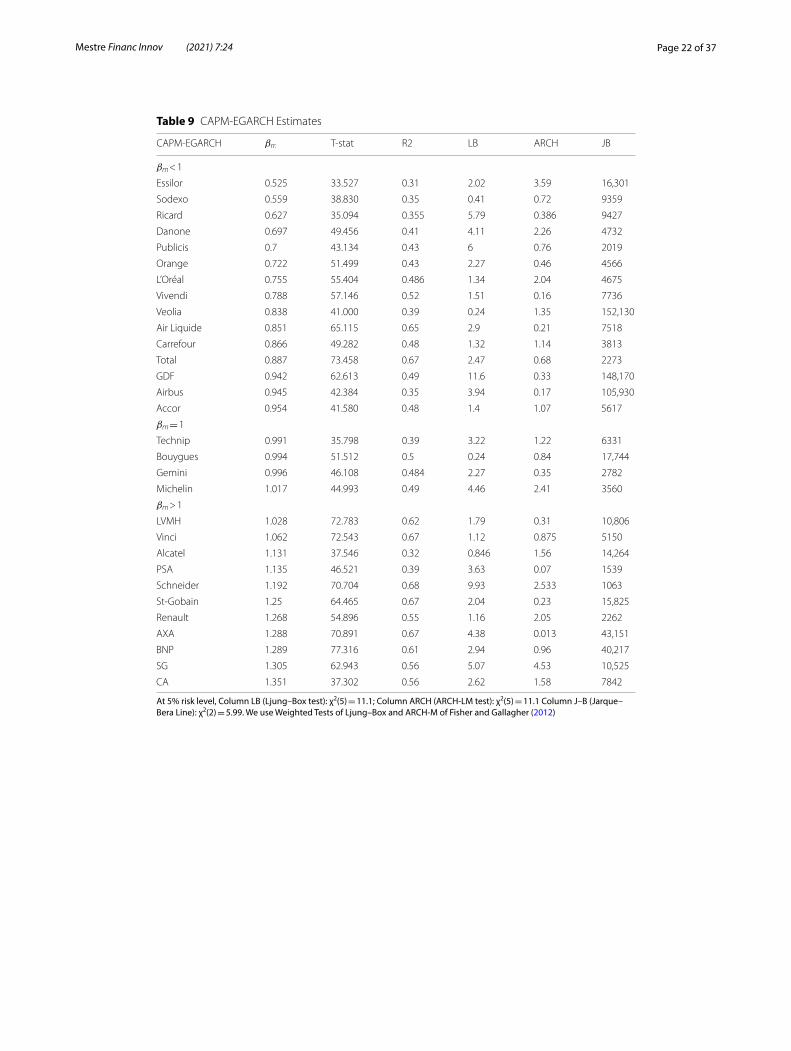
However, the presence of autocorrelational and heteroscedasticity effects in the CAPM has been observed by many authors such as Diebold et al. (1988) and Giaccoto and Ali (1982). One of the consequences of this observation is that the Beta parame-ters are inefficient. The (G)ARCH family processes of Engle (1982) and Bollerslev (1986) are currently used to estimate a Beta parameter more efficient than the OLS estimator (Bera et al. 1988; Schwert and Seguin 1990; Corhay and Rad 1996). The consideration of heteroscedasticity seems, however, to affect only periods of the high volatility of the model, as shown by Morelli (2003) by comparing two versions of CAPM (with and with-out GARCH) for U.K stocks. More recently, Bendod et al. (2017) compared the CAPM and the GARCH-CAPM for the oil sector stocks of Arab and Gulf countries and con-cluded that the EGARCH model is better adapted to estimate the Beta. Mestre and Ter-raza (2020), for French stocks, come to similar conclusions. They also specify that the beta differences (between CAPM and EGARCH-CAPM) are not very significant when Betas are less than one whereas a correction is necessary for larger betas (greater than one). For all of these studies, there is a clear improvement of the market line residuals characteristics.
We take into account the statistical limits observed in the model residuals and also agents’ heterogeneity by estimating a Multi-Betas Model with AR-EGARCH errors. We estimate 30 French stocks listed on the CAC40 (used as the Market reference) within a
Page 5 of 37Mestre Financ Innov (2021) 7:24
daily period between 2005 and 2015. We used the same database as Mestre and Terraza’s (2018) study of time–frequency CAPM and also the WTI oil price/barrel listed on the New York Mercantile Exchange, the gold price per ounce listed on the London Bullion Market, and the SMB and HML of the Fama–French Model to build a Time–Frequency based Multi-Betas Model.
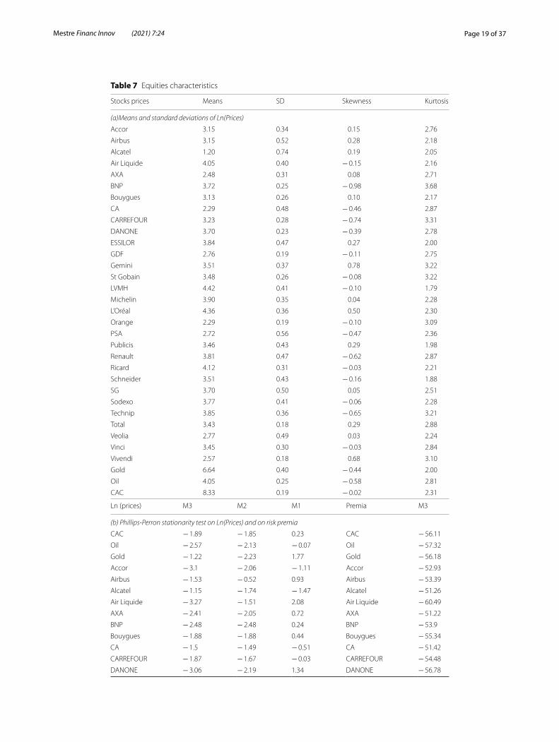
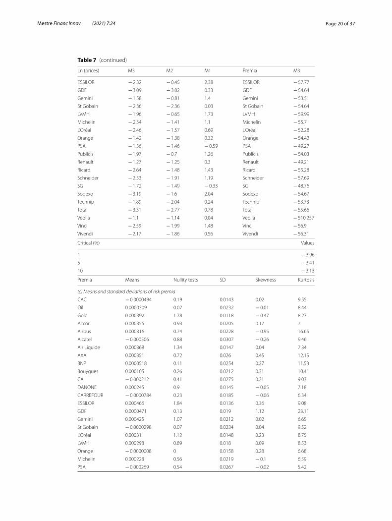
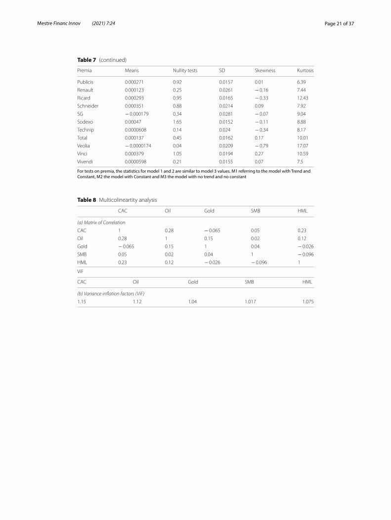
The characteristics of the series in log-form and the results of the Unit-Root Tests (see Table 7a, b) reject the stationary hypothesis. As indicated in the CAPM, the Risk Pre-mium is computed by subtracting the risk-free rate (OAT 10 years rate) from returns (the stationary variables by the first difference filter). Table 7c summarizes the char-acteristics of the risk premia series. These variables are stationary and zero-mean (see Table 7b).
The Multi-Betas Model, in its standard version (without wavelets), is written as follows:
where ri,t is the risk premium of asset i, rm,t the Market Premium, ro,tandrg ,t are Oil and Gold Premia, SMBi;t and HMLi,t are the Fama–French factors.
Under the OLS Hypothesis, εi,t is an i.i.d (0,σε ) process so in this case beta parameters are consistent estimators. The above studies reject this hypothesis concerning εi,t . As a substitute, we use the AR(1)-EGARCH(1,1) from Nelson’s (1991) study to characterize it (see Mestre and Terraza , 2020). The parameters of Eq. (1) and those of this process are simultaneously estimated by the Maximum Likelihood methods associated with a non-linear optimization algorithm (see Ye 1997; Ghalanos and Theussl 2011).
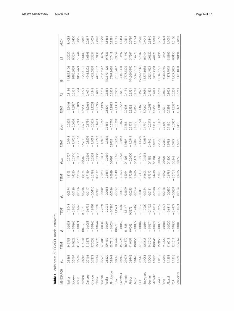
The Table 1 summarizes the Model estimations for the 30 equities ranked according to the decreasing value of the βm.
All of the Beta parameters are significant and thanks to the determination coefficients (R2), we note that the three variables explain 30–70% of assets total risks. This ranking reveals a relatively significant relationship (R2 = 0.33) between the 30 Betas βm and their corresponding determination coefficients. Equities with strong (high) βm have a glob-ally high R2 but this relationship is disrupted by the presence of outliers linked to a few stocks, as exemplified by Alcatel and PSA.
Residuals of the Multi-Betas Model are non-autocorrelated and homoscedastic, but the normality hypothesis is not respected. However, we consider this model as statisti-cally acceptable.
Significance tests of Betas are used to appreciate if the Multi-Betas Model is selected for all stocks. In this context, if βo = βg = βSMB = βHML = 0 the CAPM is selected for the stock. The overall results lead to the following comments.
We observe that the CAPM is retained for only three equities (Vivendi, Carrefour, and Schneider). Thus, the addition of other variables is not relevant because we accept βo = βg = βSMB = βHML = 0 . In this case, the CAPM results remain valid for these stocks. For the other 27 equities, there is at least one significant additional variable. For 43.33% of the stocks (13 equities) we notice a significant βo while βg is significant for 53.33% of stocks (16 equities). Finally, these two additional variables are significant for 30% of the sample (Vivendi, Total, Technip, GDF, LVMH, Alcatel, AXA, BNP, and Crédit Agricole). Concerning the Fama–French factors, βSMB is significant for 16 stocks
(1)ri,t = βm,irm,t + βo,iro,t + βg ,irg ,t + βSMB,iSMBi;t + βHML,iHMLi,t + εi,t
Page 6 of 37Mestre Financ Innov (2021) 7:24
Tabl
e 1
Mul
ti-be
tas-
AR-
EGA
RCH
mod
el e
stim
ates
MB-
EGA
RCH
βm
TSTA
T βo
TSTA
T βg
TSTA
T βSM
BTS
TAT
βHML
TSTA
T R2
JBLB
ARC
H
Essi
lor
0.54
6534
.375
5−
0.0
138
− 1
.504
80.
0374
1.81
93−
0.0
727
− 2
.194
8−
0.0
825
− 2
.644
60.
3156
14,8
86.8
106
2.29
293.
4083
Sode
xo0.
5764
34.0
822
− 0
.026
5−
3.0
530
0.01
261.
4286
− 0
.051
6−
1.4
035
− 0
.066
4−
1.8
927
0.35
2394
86.8
058
0.58
540.
7400
Rica
rd0.
6592
41.3
370
− 0
.017
1−
1.6
340
0.03
662.
2164
− 0
.093
7−
2.2
163
− 0
.224
3−
5.0
019
0.35
9484
57.2
479
5.12
440.
4965
Publ
icis
0.68
8841
.504
10.
0012
0.12
160.
0246
3.93
240.
0989
3.59
150.
0577
1.69
530.
4273
1956
.419
15.
6180
0.68
82
Dan
one
0.71
0151
.337
3−
0.0
053
− 0
.673
50.
0147
0.71
69−
0.0
294
− 0
.857
6−
0.1
754
− 6
.206
40.
4071
4941
.322
23.
6895
2.02
17
Ora
nge
0.73
7147
.565
2−
0.0
145
− 1
.840
1−
0.0
410
− 2
.279
8−
0.0
524
− 1
.701
9−
0.0
855
− 3
.126
80.
4348
4729
.682
02.
3237
0.40
09
L’Oré
al0.
7862
56.3
575
− 0
.024
2−
3.3
899
0.00
710.
5172
− 0
.098
8−
2.9
723
− 0
.166
3−
5.9
745
0.48
9244
28.9
182
1.94
312.
4978
Vive
ndi
0.79
2257
.310
8−
0.0
080
− 2
.279
1−
0.0
103
− 2
.984
5−
0.0
033
− 1
.509
2−
0.0
262
− 6
.198
90.
5234
7736
.551
21.
6092
0.15
86
Veol
ia0.
8520
40.4
459
− 0
.029
7−
2.2
036
− 0
.025
3−
0.9
384
− 0
.063
9−
2.7
895
0.03
850.
8809
0.38
8815
2,57
3.15
250.
7125
11.8
468
Air
Liqu
ide
0.85
4163
.721
6−
0.0
034
− 0
.788
60.
0386
3.09
390.
0792
2.97
55−
0.0
770
− 2
.803
30.
6509
7907
.845
02.
7418
0.32
81
Tota
l0.
8663
78.3
249
0.07
7011
.159
30.
0772
6.71
49−
0.0
776
− 3
.923
0−
0.0
260
− 2
.133
30.
6953
2313
.844
72.
9854
1.11
12
Carr
efou
r0.
8769
45.7
226
− 0
.015
9−
1.8
985
− 0
.001
5−
0.3
979
− 0
.022
8−
0.5
863
− 0
.002
3−
0.0
567
0.48
3738
07.5
330
1.36
921.
1464
Tech
nip
0.91
7836
.457
90.
1388
11.1
147
0.10
294.
5024
0.11
051.
9307
0.12
862.
0498
0.41
3976
78.6
395
5.16
974.
9311
Airb
us0.
9448
41.6
451
0.00
450.
5873
0.02
133.
7259
− 0
.040
0−
1.0
343
0.05
752.
5552
0.35
5110
4,36
6.39
803.
7567
0.07
94
Acc
or0.
9446
40.8
456
− 0
.017
7−
1.4
160
0.03
541.
2486
0.14
713.
4207
0.06
251.
2867
0.47
8856
69.3
152
1.67
731.
1744
GD
F0.
9966
127.
1810
− 0
.018
2−
3.3
635
− 0
.041
6−
3.7
110
− 0
.091
9−
1.4
589
− 0
.072
8−
1.4
691
0.49
7715
0,61
2.73
685.
7682
0.19
08
Bouy
gues
0.99
5140
.363
5−
0.0
194
− 1
.790
00.
0384
2.46
03−
0.1
034
− 3
.161
70.
1739
3.99
690.
5050
18,3
77.1
038
0.54
540.
4945
Gem
ini
1.00
4244
.301
0−
0.0
274
− 2
.142
50.
0181
0.73
730.
1185
2.44
46−
0.0
315
− 0
.608
70.
4855
2924
.406
32.
6322
0.38
40
Mic
helin
1.01
3649
.084
6−
0.0
229
− 1
.851
70.
0370
1.44
200.
1794
3.95
250.
0932
1.85
070.
4899
3228
.750
84.
0973
1.28
92
LVM
H1.
0319
75.9
458
− 0
.012
8−
1.9
659
0.01
852.
2401
0.05
672.
2029
− 0
.030
7−
1.4
042
0.62
5010
,589
.679
11.
6496
0.71
56
Vinc
i1.
0595
74.3
620
− 0
.018
3−
1.8
476
0.01
481.
0902
0.06
011.
2580
0.03
060.
9531
0.66
9550
88.6
765
1.34
541.
0304
Alc
atel
1.12
5541
.601
5−
0.0
220
− 0
.631
2−
0.0
530
− 0
.678
10.
1500
1.97
810.
1130
0.78
560.
3928
1578
.797
53.
8509
1.10
19
PSA
1.13
1832
.161
1−
0.0
236
− 2
.447
9−
0.0
831
− 2
.573
30.
2242
4.09
79−
0.0
907
− 1
.332
70.
3258
13,9
27.3
025
0.91
501.
3106
Schn
eide
r1.
1898
67.4
567
− 0
.010
3−
1.0
074
0.01
941.
0206
0.06
591.
6223
0.04
161.
0323
0.67
6311
28.1
090
9.81
942.
4801
Page 7 of 37Mestre Financ Innov (2021) 7:24
At 5
% s
igni
fican
ce le
vel,
Colu
mn
LB (L
jung
–Box
test
): χ2 (5
) = 1
1.1;
Col
umn
ARC
H (
ARC
H-L
M te
st):
χ2 (5) =
11,
1 Co
lum
n J–
B (J
arqu
e–Be
ra L
ine)
: χ2 (2
) = 5
,99.
We
use
Wei
ghte
d Te
sts
of L
jung
–Box
and
ARC
H-M
of F
ishe
r and
G
alla
gher
(201
2). M
oreo
ver,
in th
is m
odel
the
non-
colli
near
ity b
etw
een
exog
eneo
us v
aria
bles
are
test
ed (s
ee T
able
8).
The
nam
es o
f cer
tain
act
ions
are
abb
revi
ated
, see
the
list o
f abb
revi
atio
ns fo
r mor
e de
tails
on
thei
r ful
l na
me
Tabl
e 1
(con
tinue
d)
MB-
EGA
RCH
βm
TSTA
T βo
TSTA
T βg
TSTA
T βSM
BTS
TAT
βHML
TSTA
T R2
JBLB
ARC
H
St-G
obai
n1.
2373
69.2
948
− 0
.002
6−
0.3
686
0.00
560.
5795
0.17
075.
7325
0.05
511.
3654
0.66
9316
,152
.700
32.
6272
0.21
83
Rena
ult
1.26
0251
.717
2−
0.0
200
− 1
.439
50.
0157
0.60
350.
1284
2.33
790.
0978
1.43
160.
5498
2219
.414
11.
1933
1.91
39
AXA
1.28
9367
.077
6−
0.0
444
− 4
.408
7−
0.0
577
− 2
.923
0−
0.0
733
− 1
.764
90.
2083
4.55
340.
6726
45,9
09.1
043
5.03
980.
0089
BNP
1.29
2564
.248
3−
0.0
405
− 3
.957
7−
0.0
827
− 5
.173
0−
0.0
317
− 0
.754
50.
2717
5.97
550.
6185
40,0
68.3
805
2.46
140.
5333
SG1.
3068
27.7
305
− 0
.008
7−
0.7
971
− 0
.095
5−
3.7
482
− 0
.027
4−
1.1
462
0.30
065.
9691
0.56
7410
,487
.573
85.
0467
4.50
46
CA
1.32
6255
.429
7−
0.0
332
− 3
.500
0−
0.0
812
− 3
.392
90.
0003
0.00
550.
4087
6.24
930.
5679
7916
.505
41.
9223
1.99
58
Page 8 of 37Mestre Financ Innov (2021) 7:24
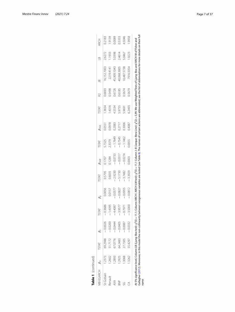
(53.33% of the sample) and βHML for 15 (50%). They are both significant for five equities (Essilor, Ricard, L’Oréal, Air Liquide, and Total, Bouygues).
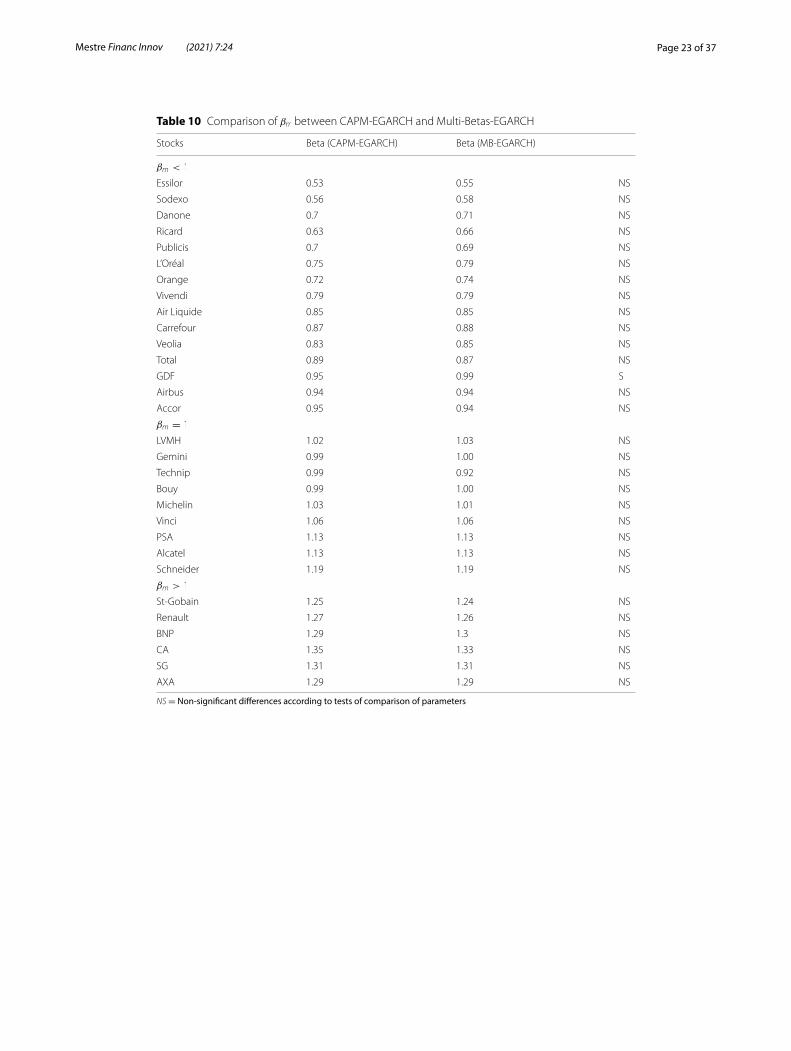
We built an adjustment of OLS Betas in order to quickly appreciate a more consistent βm without reestimating the model with AR(1)-EGARCH1 processes. This adjustment remains valid in the case of the Multi-Betas Model, because we observe no significant differences between the βm (and residuals) of Multi-Betas Model in Table 2 and the βm of a CAPM with AR(1)-EGARCH(1,1) errors (see Tables 9, 10). The addition of these addi-tional variables has a limited impact on the vast majority of equities because the βm are not affected. However, the Multi-Betas Model results have an interest to portfolio man-agers for analyzing and interpreting the βo and βg (their sign and their value) illustrating the sensitivities to oil and gold fluctuations.
For a large part of equities having a significant βo , we notice that estimators are almost negative, however, sensitivities to oil movements are relatively low varying between − 0.001 and − 0.045%. Considering the classification of stocks by βm , as in Table 1, we observe that oil affects the different equities profiles in the same way. Technip and Total are a notable exception to this case because their βo have higher positive values com-pared to the other stocks. Thereby, an oil price rise by 1% entails a stock price rise by 0.08% for Total and by 0.14% for Technip. We conclude that stocks of the oil and gas sec-tors are the most sensitive to oil price fluctuations, which is relevant to their activities.
We note significant and negative βg for seven stocks (Alcatel, SG, BNP, CA, AXA, Orange, Vivendi, and GDF) and positive for seven others equities (Publicis, Essilor, Ricard, Air Liquide, Bouygues, Total, and Technip). The Financial sector equities, clas-sified as “risky” due to their βm greater than one, are negatively affected by the gold, jus-tifying in part its “safe haven” characteristic. We can extend this result to stocks with strong βm (Financial Sector + Alcatel) having a negative and relatively higher sensitivity to gold fluctuations. On the contrary, stocks with βm < 1 have positive and lower βg . Once again, Total and Technip are exceptions because they are more sensitive to gold than other stocks.
By comparing these three sensitivity estimators, the market represents a major source of risk because the βm are greater than βg and βo in absolute values. We also note that Gold sensitivity is higher (in absolute values) than oil sensitivity, particularly in financial sectors and for stocks with βm > 1.
Time–frequency multi‑betas model estimatesIn the financial markets, the assumption of homogeneity of agents’ behavior is dif-ficult to maintain. The investment frequency of a global and a mutual funds portfolio, for example, depends on their buying or selling intentions based on various calcula-tion/financial models. These models don’t differentiate the agents and considers only an aggregation of behaviors (i.e. an “average behavior”) from the financial time series used. The use of wavelet time–frequency decompositions of these time series is justified in the Multi-Betas Model framework because the high-frequencies are related to HFT and the low-frequencies to fundamentalist investors. Wavelets represent a relevant solution to
1 See Mestre and Terraza (2020).
Page 9 of 37Mestre Financ Innov (2021) 7:24
analyzing the behavior of agents that use this kind of financial model. In the rest of the paper, we name Standard Multi-Beta Models, the results of which are summarized in Table 1, to distinguish from its time–frequency versions estimated in this section.
The first paragraph is a brief reminder of wavelets methodology applied to our model before comparing results obtained in the previous part for the Standard Multi-Betas Model with its time–frequency version in the second paragraph. In a third paragraph, we analyse the frequency sensitivities of stock prices to exogenous additional variables.
Wavelets methodology reminder: the maximal overlap discrete wavelets transform (or MODWT):
A Wavelets-mother �(t) with zero-mean and normalised is written as follows2:
These properties ensure the Variance/Energy preservation during the decomposition of a series and also guarantee the respect of admissibility condition (Grossman and Mor-let 1984).
This wavelet-mother is shifted by the τ parameter and dilated by scale parameters to create “wavelets-daughters’’ regrouping in the wavelets family used as filtering basis:
The decomposition of time function x(t) creates/lead to the wavelets coefficients W (s, τ) as follows:
τ and s parameters indicate the time and frequency localization of the coefficient. Thanks to the wavelets, we can represent the temporal localization of the frequency components, hence the name of the time–frequency analysis. These previous equations are a theoretical presentation of wavelet decompositions based on continuous wavelets. A time discreet version is used to decompose time series xt but the principle remains
(2)+∞∫
−∞ψ(t)dt = 0 and
+∞∫
−∞|ψ(t)|2dt = 1
(3)�τ,s(t) =1√s�
(
t− τ
s
)
(4)W (s, τ) =
+∞∫
−∞x(t)
1√sψ∗
(
t − τ
s
)
dt =< x(t),ψτ ,s(t) >
ψ∗ is the complex conjuguate of ψ
Table 2 Percentages of significantly different Betas between Standard Multi-Betas Model and Time–Frequency Multi-Betas Model (TFMB)
We test if the difference between the two estimators are significant with Student Test. We count the number of significant differences and we expressed them as a percentage of the total number of actions (i.e. 30)
D1 (%) D2 (%) D3 (%) D4 (%) D5 (%) D6 (%)
βm 13.33 13.33 33.33 56.67 66.67 76.67
βo 16.67 23.33 40.00 46.67 70.00 83.33
βg 6.67 6.67 23.33 46.67 66.67 73.33
βSMB 23.33 13.33 26.67 40.00 40.00 66.67
βHML 13.33 13.33 33.33 50.00 70.00 63.33
2 We use the notation of Mallat (2001).
Page 10 of 37Mestre Financ Innov (2021) 7:24
similar because frequencies are still continuous. The practical use of this kind of decom-position implies important computational time and effort, consequently, a frequency discretization is realized for a fast-decomposing time series, as is the MODWT. In this framework, wavelets are defined by a succession repeated J times of high-pass and low-pass filter combinations (Mallat Algorithm 1989, 2009). J is the decomposition order representing the optimal number of repetitions necessary to reconstruct a time series xt of length N such as J = Ln(N)
Ln(2) .Despite this simplified process, the MODWT is still variance/energy preserving. It
ensures the perfect reconstruction of the decomposed series, without losses, by adding the high and low-frequencies components:
SJ,t is a basic approximation of the series and Dj,t are the details, called also frequency bands, of scale j regrouping the frequencies in the interval
[
12
j+1; 12
j]
.
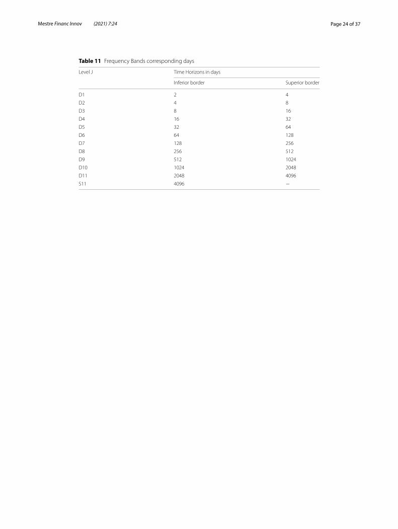
In Finance, the frequencies interpretation is simplified by translating them in periods that have the same time unit as the original data (for example, days, weeks, etc.). In this case, frequencies represent the different time investment horizons (short-medium-long run). The Table 11 records the frequency bands and the corresponding time horizons in days.
Considering the series length, through wavelets decomposition, we have 11 frequency bands and one approximation. The high-frequencies bands (D1–D2) are related to short-run investments whereas the low-frequencies illustrate long-run horizons. In order to simplify the analysis, we focus on the first six frequency bands: D1 bands are related to 2–4 days investment horizon (high-frequencies) whereas D6 band represents a 3–6 month investment (low-frequencies).
In the Multi-Betas Model framework, we decompose the dependent and the three independent variables by the MODWT. In the Multi-Betas Model, each frequency band of the stock are associated with the corresponding bands of the market, oil, gold, and Fama–French factors. By construction, the frequency bands means are equal to zero.
For an asset i, the Time–Frequency Multi-Betas Model is written as follows:
Betas parameters are estimated in the time–frequency space and represent the asset sensitivities to the five factors considering agents’ investment frequencies and consider-ing stock risk profiling. The different time–frequency regression models are estimated previously by conserving the hypothesis of AR(1)-EGARCH(1,1) errors.
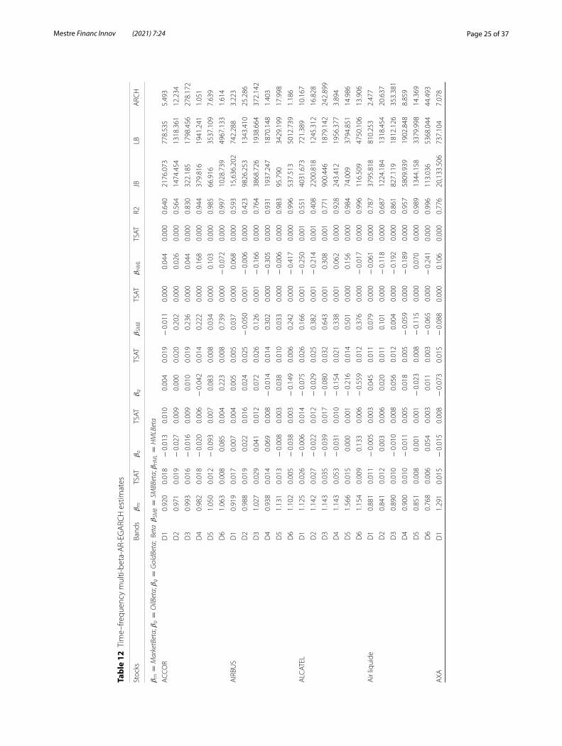
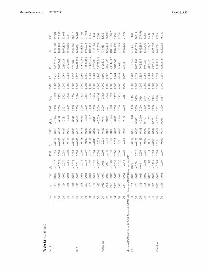
Table 12 summarizes all results3 of Time–Frequency Multi-Betas AR-EGARCH Model estimates.
(5)xt = SJ,t +j=J∑
j=1
Dj,t
(6)Dassetj,t = βm
j DMarketj,t + βo
j DOilj,t + β
gj D
Goldj,t + βSMB
j DSMBj,t + βHML
j DHMLj,t + εj,t
∀j = 1, . . . , 6the frequency band
εj,t ∼ AR(1)− EGARCH(1, 1)
3 We use the ‘’rugarch’’ R—package developed by Ghalanos and Theussl (2011).
Page 11 of 37Mestre Financ Innov (2021) 7:24
Time–frequency multi-betas model estimatesβm coefficients are highly significant for all equities and frequencies. The coefficients
of determination computed on the high-frequencies (D1–D2) are relatively closed to the overall Model of Table 1. But they become more important for medium–low-frequencies (D4–D5) and they are almost equal to 100% on the D6 band. The order of magnitude of the D5–D6 wavelets coefficients are small, therefore, a range of residuals estimates are also small, and then values of R2 are high on low-frequencies. However, for all frequency band regressions, we notice a deterioration of residual characteristics. Particularly, the AR-EGARCH process no longer properly captures the heteroscedasticity. By increasing the order of the process, we reduce the autocorrelation and heteroscedasticity without significantly modifying the values of the Betas parameters. Despite these reservations, the Time–Frequency Multi-Betas Model has sufficient statistical properties to analyze its economic results.
Estimates of these parameters play an important role in investor strategies who ques-tion the choice of the model according to the significant parameters. Globally, we remark that stocks with a strong βm (> 1) have negative βo and βg for all frequency bands more particularly in the long-run. The stocks with low βm (< 1) have positive and relatively high βg whereas βo still mainly remain negative. Portfolio managers can thus appreciate the different sources of risk affecting their portfolios when making choices.
Table 2 summarizes the differences between parameters of standard and time–fre-quency models and represents an additional help to interpret results.
The Betas estimated without wavelets (Standard Multi-Betas) are globally similar to short-run Betas (D1–D2) for the majority of equities whereas the differences are more significant in the long-run. For example, in the long-run (D6), we note that differences between βm of the Standard Model and TFMB are significant for 76.67% of equities.
Wavelets provide a differentiated beta estimate according to the investment frequen-cies, which are useful for identifying and analyzing the effects of investment horizons on systematic risk measures/indicators and on sensitivities to different factors. The intensity of βo and βg is greater in the long-run than in the short-run. For all equities, the selected variables more strongly affect assets for long-run investments. Therefore, we confirm the results of Gençay et al. (2005) as well as Mestre and Terraza (2018) concerning the inter-est of wavelets in market models for long-run investments. Both studies indicated that CAPM’s Beta is frequency-varying for long-run investment horizons and the standard estimation of Beta does not hold. Therefore, equities risk profile changes. The Time–Fre-quency Multi-Betas Model is therefore of strategic interest for long-term investments by estimating its low-frequency exposures to risks in order to adjust their allocation if the initial characteristic is lost (see Part III).
Stocks sensitivities to oil and gold movementsBy testing the significance of frequency parameters βo,βg ,βSMB and βHML for all
stocks, we establish the following statements:
• If βo = βg = βSMB = βHML = 0 , the addition of the four variables is not appropriate for this asset. In this case, the time–frequency CAPM4 is selected.
4 The time–frequency CAPM is already estimated in the study Mestre and Terraza (2018).
Page 12 of 37Mestre Financ Innov (2021) 7:24
• If βo = 0,βg = 0,βSMB = 0 and βHML = 0 the five additional variables are relevant and the Full Multi-Betas Model (FULL MB) is retained.
• If βo = 0,βg = 0,βSMB = 0 and βHML = 0, only two additional variables are rel-evant and the Multi-Betas Model with Oil and Gold (MB OIL GOLD) is retained.
• If βo = 0, βg = 0, βSMB �= 0 and βHML �= 0, only Fama–French factors are relevant and the Fama–French Model (FF) is retained.
• If at least one of the five Beta is significant, we always retain the Multi-Betas Model under a mixed version.
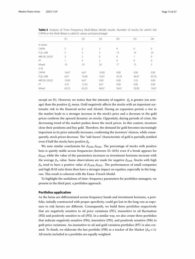
We use this framework to summarize results in the Tables 3 and 13. We count for each frequency band the number of shares for which the CAPM or Multi-Betas is retained.
By reading Tables 3 and 12 in Appendix, it is possible to establish the following com-ments:
• There is no stocks having the CAPM on all frequency bands, while lot of equities retained a version of Multi-Betas Model whatever the investment horizon.
• In the short-run (D1), the CAPM is valid for only five stocks (16.66% of the sample) and results are similar to the previous estimate of the Standard Model. This percent-age decreases as the time horizon increase, so more stocks retain the Full Multi-Betas Model in the long-run. After D3 bands, there are no equities having non-significant additional variables. Stocks are therefore more impacted/affected by oil and/or gold in the long-term than in the short-term as the Fama–French Factors affected a large part of stocks.
The Time Frequency Multi-Betas Model is therefore of statistical interest for a major-ity of equities whatever the investment horizons. This model is complementary to the CAPM results as it introduces the decompositions of risk sources. It can be decision-making support for investors by synthesizing the results of the stock sensitivities.
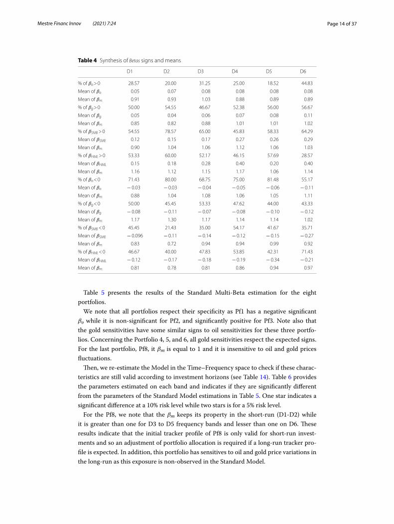
Table 4 synthesizes, for each frequency band, the percentage of βo,βg ,βSMB,βHML sig-nificantly greater, lower, or equal to zero and also their means. To improve the analysis, we also indicate the mean of the corresponding βm.
The number of Multi-Betas Model having a positive βg is relatively stable on all fre-quency bands (around 50%) whereas it increases for the model with positive βo. Further-more, we note that their means increase from D1 (short-run) to D6 (long-run). Stocks with positive βg and/or positive β0 have an average βm less or equal to one. The oil-sector stocks (Total, Technip) are strongly and positively sensitive to oil and gold for all frequency bands.
The number of stocks negatively sensitive to oil is higher in the short-term (D1–D2) than the long-term (D6), whereas it is stable for gold. The value of βg and β0 increases as the investment horizon increases (in average). We note similar results for stocks with βo < 0 as the mean of βm increases accross frequencies, it is less than one until the D3-Bands but is greater beyond. Financial Equities (SG, BNP, CA, and AXA) are not sen-sitive to oil short-run variations. However, these stocks have strongly negative βo when investment horizon increases (D5-D6). Financial stocks are also strongly negatively affected by gold prices both in the short- and long-run, however, the effect is greater. The equities are negatively sensitive to gold, which has an average βm greater than one
Page 13 of 37Mestre Financ Innov (2021) 7:24
Table 3 Analysis of Time–Frequency Multi-Betas Model results. Number of stocks for which the CAPM or the Multi-Betas is valid (in values and percentage)
D1 D2 D3 D4 D5 D6
In values
CAPM 5 2 3 0 0 0
FULL MB 2 3 5 13 14 25
MB OIL GOLD 3 2 0 0 1 0
FF 1 4 2 0 0 0
Mixed 19 19 20 17 15 5
In %
CAPM 16.67 6.67 10.00 0.00 0.00 0.00
FULL MB 6.67 10.00 16.67 43.33 46.67 83.33
MB OIL GOLD 10.00 6.67 0.00 0.00 3.33 0.00
FF 3.33 13.33 6.67 0.00 0.00 0.00
Mixed 63.33 63.33 66.67 56.67 50.00 16.67
except on D1. However, we notice that the intensity of negative βg is greater (on aver-age) than the positive βg mean. Gold negatively affects the stocks with an important sys-tematic risk in the financial sector and Alcatel. During an expansion period, a rise in the market leads to a stronger increase in the stock’s price and a decrease in the gold prices confirms the upward dynamic on stocks. Oppositely, during periods of crisis, the decreasing trend of the market pushes down the stock prices. In this context, investors close their positions and buy gold. Therefore, the demand for gold becomes increasingly important as its price naturally increases, confirming the investors’ choices, while conse-quently, stock prices decrease. The “safe haven” characteristic of gold is partially justified even if half the stocks have positive βg .
We note similar conclusions for βSMB,βHML . The percentage of stocks with positive beta is quietly stable across frequencies (between 55–65%) even if a break appears for βHML while the value of the parameters increases as investment horizons increase with the average βm value. Same observations are made for negative βSMB . Stocks with high βm tend to have a positive value of βSMB,βHML . The performances of small companies and high B/M ratio firms then have a stronger impact on equities, especially in the long-run. This result is coherent with the Fama–French Model.
To highlight the usefulness of time–frequency parameters for portfolios managers, we present in the third part, a portfolios approach.
Portfolios applicationAs the betas are differentiated across frequency bands and investment horizons, a port-folio, initially constructed with proper specificity, could get lost in the long-run as expo-sure to risk factors are different. Consequently, we build three portfolios respectively that are negatively sensitive to oil price variations (Pf1), insensitive to oil fluctuation (Pf2) and positively sensitive to oil (Pf3). In a similar way, we also create three portfolios that indicate negatively sensitive (Pf4), insensitive (Pf5), and positively sensitive (Pf6) to gold price variations. An insensitive to oil and gold variation portfolios (Pf7) is also cre-ated. To finish, we elaborate the last portfolio (Pf8) as a tracker of the Market ( βm = 1). All stocks included in a portfolio are equally weighted.
Page 14 of 37Mestre Financ Innov (2021) 7:24
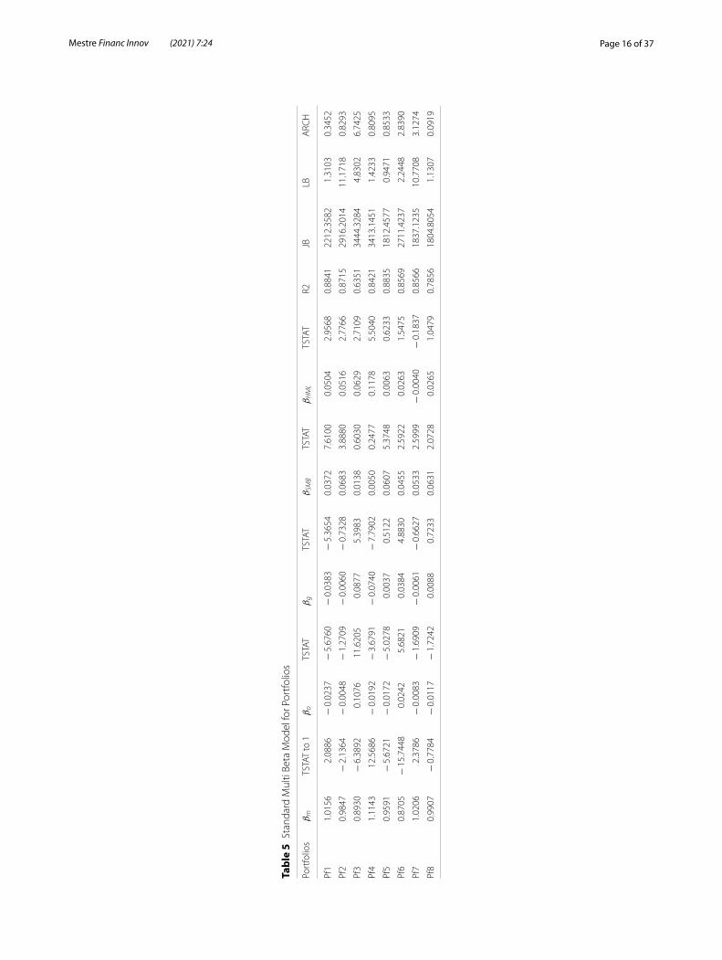
Table 5 presents the results of the Standard Multi-Beta estimation for the eight portfolios.
We note that all portfolios respect their specificity as Pf1 has a negative significant βo while it is non-significant for Pf2, and significantly positive for Pf3. Note also that the gold sensitivities have some similar signs to oil sensitivities for these three portfo-lios. Concerning the Portfolio 4, 5, and 6, all gold sensitivities respect the expected signs. For the last portfolio, Pf8, it βm is equal to 1 and it is insensitive to oil and gold prices fluctuations.
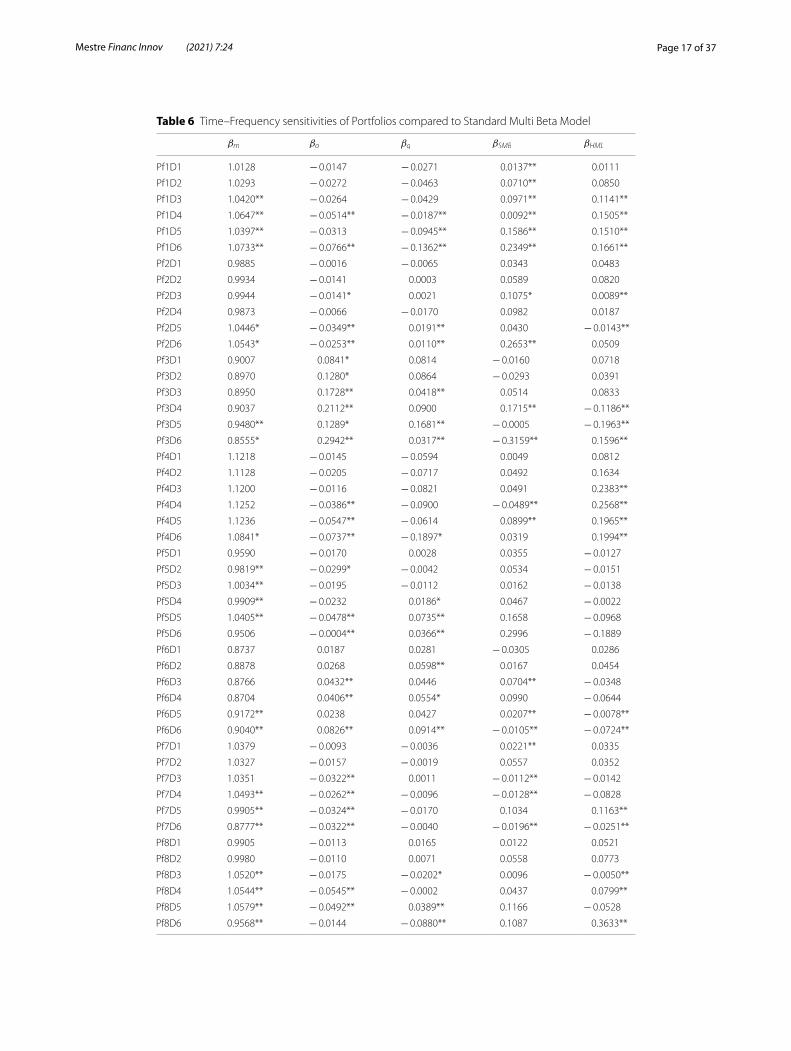
Then, we re-estimate the Model in the Time–Frequency space to check if these charac-teristics are still valid according to investment horizons (see Table 14). Table 6 provides the parameters estimated on each band and indicates if they are significantly different from the parameters of the Standard Model estimations in Table 5. One star indicates a significant difference at a 10% risk level while two stars is for a 5% risk level.
For the Pf8, we note that the βm keeps its property in the short-run (D1-D2) while it is greater than one for D3 to D5 frequency bands and lesser than one on D6. These results indicate that the initial tracker profile of Pf8 is only valid for short-run invest-ments and so an adjustment of portfolio allocation is required if a long-run tracker pro-file is expected. In addition, this portfolio has sensitives to oil and gold price variations in the long-run as this exposure is non-observed in the Standard Model.
Table 4 Synthesis of Betas signs and means
D1 D2 D3 D4 D5 D6
% of βo > 0 28.57 20.00 31.25 25.00 18.52 44.83
Mean of βo 0.05 0.07 0.08 0.08 0.08 0.08
Mean of βm 0.91 0.93 1.03 0.88 0.89 0.89
% of βg > 0 50.00 54.55 46.67 52.38 56.00 56.67
Mean of βg 0.05 0.04 0.06 0.07 0.08 0.11
Mean of βm 0.85 0.82 0.88 1.01 1.01 1.02
% of βSMB > 0 54.55 78.57 65.00 45.83 58.33 64.29
Mean of βSMB 0.12 0.15 0.17 0.27 0.26 0.29
Mean of βm 0.90 1.04 1.06 1.12 1.06 1.03
% of βHML > 0 53.33 60.00 52.17 46.15 57.69 28.57
Mean of βHML 0.15 0.18 0.28 0.40 0.20 0.40
Mean of βm 1.16 1.12 1.15 1.17 1.06 1.14
% of βo < 0 71.43 80.00 68.75 75.00 81.48 55.17
Mean of βo − 0.03 − 0.03 − 0.04 − 0.05 − 0.06 − 0.11
Mean of βm 0.88 1.04 1.08 1.06 1.05 1.11
% of βg < 0 50.00 45.45 53.33 47.62 44.00 43.33
Mean of βg − 0.08 − 0.11 − 0.07 − 0.08 − 0.10 − 0.12
Mean of βm 1.17 1.30 1.17 1.14 1.14 1.02
% of βSMB < 0 45.45 21.43 35.00 54.17 41.67 35.71
Mean of βSMB − 0.096 − 0.11 − 0.14 − 0.12 − 0.15 − 0.27
Mean of βm 0.83 0.72 0.94 0.94 0.99 0.92
% of βHML < 0 46.67 40.00 47.83 53.85 42.31 71.43
Mean of βHML − 0.12 − 0.17 − 0.18 − 0.19 − 0.34 − 0.21
Mean of βm 0.81 0.78 0.81 0.86 0.94 0.97
Page 15 of 37Mestre Financ Innov (2021) 7:24
For Pf1 (initially negatively sensitive to oil), it conserves this characteristic for all fre-quencies, but this initial exposure is significantly greater in the long-run. A similar result is noted for Pf3 (initially positively sensitive to gold) as the sensitivities are significantly greater in the long-run than in the short-run. The Pf2 keeps its insensitive property until D4 bands but not in the long-run as it becomes negatively sensitive to oil (and positively to gold). We also observe similar conclusions concerning the sensitivities to Gold for these three portfolios.
For Pf4, the initial profile with negative βg is conserved no matter the investment hori-zons, but in the long-run, its exposure to gold is significantly greater than estimated by the Standard Model. Similar observations are noted for the Pf6, however for some hori-zons, the sensitivity is greater than estimated in Table 5. Results for a gold insensitive portfolio (Pf5) highlight significant difference between parameters on D2, D4 and D6 frequency bands as βg is positive.
Concerning the Pf7, initially non sensitive to oil and gold, the insensitive characteristic is lost as the βo is significantly negative starting D3 bands even if βg is still equal to 0. To conserve this property for long-run investments, a new allocation is required.
For all portfolios, we note a differentiation of parameters across frequency bands con-firming previous observations.
The results obtained by wavelet estimators of risks sensibilities are useful for inves-tors to support their decision-making on portfolio allocation and could be completed by multiple criteria decisions making (MCDM) methods and clusters algorithms based on different risks measured in the assessment of financial risks or in predictions of variables (Kou et al. 2014, 2021).
ConclusionThe Time–Frequency Multi-Betas Model effectively complements the different instru-ments used by stock investors to build their portfolios. In the first hand, it can substitute the CAPM by considering the residual anomalies by using ARMA-EGARCH processes to model the errors of the regression. On the other hand, it improves the CAPM by add-ing exogeneous variables and it considers the heterogeneity of agents’ behaviors by the wavelet decompositions. Despite some statistical shortcomings, particularly those con-cerning the characteristics of its frequency residuals, this model brings a significant gain of information to model the risk premiums.
In the short-run, the βm parameter of the Time–Frequency Multi-Betas Model, meas-uring the sensitivity to market fluctuation, is not significantly different to the Standard Multi-Betas Model and the CAPM. For a short-run investor, the use of the CAPM can be sufficient to make investment choices based on the βm . However, he can consider the Multi-Betas Model and the sensitivities to gold and oil in order to modulate its choices.
The Standard Multi-Betas Model (without wavelets) is retained for a majority of the stocks in its full or one mixed version. The stock sensitivities to oil and gold are lower than the sensitivity to the market, but we can appreciate potential positive effects on some sectors such as the Petroleum/Gaz-stocks, and Financial sectors. For example, oil negatively affects the majority of stocks, however, its impact is stronger for high βm equi-ties than low βm equities. Gold negatively and more strongly affects equities with a high systematic risk (such as the Financial sector) but the effect is reversed for equities with a
Page 16 of 37Mestre Financ Innov (2021) 7:24
Tabl
e 5
Stan
dard
Mul
ti Be
ta M
odel
for P
ortfo
lios
Port
folio
sβm
TSTA
T to
1βo
TSTA
T βg
TSTA
T βSM
BTS
TAT
βHML
TSTA
T R2
JBLB
ARC
H
Pf1
1.01
562.
0886
− 0
.023
7−
5.6
760
− 0
.038
3−
5.3
654
0.03
727.
6100
0.05
042.
9568
0.88
4122
12.3
582
1.31
030.
3452
Pf2
0.98
47−
2.1
364
− 0
.004
8−
1.2
709
− 0
.006
0−
0.7
328
0.06
833.
8880
0.05
162.
7766
0.87
1529
16.2
014
11.1
718
0.82
93
Pf3
0.89
30−
6.3
892
0.10
7611
.620
50.
0877
5.39
830.
0138
0.60
300.
0629
2.71
090.
6351
3444
.328
44.
8302
6.74
25
Pf4
1.11
4312
.568
6−
0.0
192
− 3
.679
1−
0.0
740
− 7
.790
20.
0050
0.24
770.
1178
5.50
400.
8421
3413
.145
11.
4233
0.80
95
Pf5
0.95
91−
5.6
721
− 0
.017
2−
5.0
278
0.00
370.
5122
0.06
075.
3748
0.00
630.
6233
0.88
3518
12.4
577
0.94
710.
8533
Pf6
0.87
05−
15.
7448
0.02
425.
6821
0.03
844.
8830
0.04
552.
5922
0.02
631.
5475
0.85
6927
11.4
237
2.24
482.
8390
Pf7
1.02
062.
3786
− 0
.008
3−
1.6
909
− 0
.006
1−
0.6
627
0.05
332.
5999
− 0
.004
0−
0.1
837
0.85
6618
37.1
235
10.7
708
3.12
74
Pf8
0.99
07−
0.7
784
− 0
.011
7−
1.7
242
0.00
880.
7233
0.06
312.
0728
0.02
651.
0479
0.78
5618
04.8
054
1.13
070.
0919
Page 17 of 37Mestre Financ Innov (2021) 7:24
Table 6 Time–Frequency sensitivities of Portfolios compared to Standard Multi Beta Model
βm βo βg βSMB βHML
Pf1D1 1.0128 − 0.0147 − 0.0271 0.0137** 0.0111
Pf1D2 1.0293 − 0.0272 − 0.0463 0.0710** 0.0850
Pf1D3 1.0420** − 0.0264 − 0.0429 0.0971** 0.1141**
Pf1D4 1.0647** − 0.0514** − 0.0187** 0.0092** 0.1505**
Pf1D5 1.0397** − 0.0313 − 0.0945** 0.1586** 0.1510**
Pf1D6 1.0733** − 0.0766** − 0.1362** 0.2349** 0.1661**
Pf2D1 0.9885 − 0.0016 − 0.0065 0.0343 0.0483
Pf2D2 0.9934 − 0.0141 0.0003 0.0589 0.0820
Pf2D3 0.9944 − 0.0141* 0.0021 0.1075* 0.0089**
Pf2D4 0.9873 − 0.0066 − 0.0170 0.0982 0.0187
Pf2D5 1.0446* − 0.0349** 0.0191** 0.0430 − 0.0143**
Pf2D6 1.0543* − 0.0253** 0.0110** 0.2653** 0.0509
Pf3D1 0.9007 0.0841* 0.0814 − 0.0160 0.0718
Pf3D2 0.8970 0.1280* 0.0864 − 0.0293 0.0391
Pf3D3 0.8950 0.1728** 0.0418** 0.0514 0.0833
Pf3D4 0.9037 0.2112** 0.0900 0.1715** − 0.1186**
Pf3D5 0.9480** 0.1289* 0.1681** − 0.0005 − 0.1963**
Pf3D6 0.8555* 0.2942** 0.0317** − 0.3159** 0.1596**
Pf4D1 1.1218 − 0.0145 − 0.0594 0.0049 0.0812
Pf4D2 1.1128 − 0.0205 − 0.0717 0.0492 0.1634
Pf4D3 1.1200 − 0.0116 − 0.0821 0.0491 0.2383**
Pf4D4 1.1252 − 0.0386** − 0.0900 − 0.0489** 0.2568**
Pf4D5 1.1236 − 0.0547** − 0.0614 0.0899** 0.1965**
Pf4D6 1.0841* − 0.0737** − 0.1897* 0.0319 0.1994**
Pf5D1 0.9590 − 0.0170 0.0028 0.0355 − 0.0127
Pf5D2 0.9819** − 0.0299* − 0.0042 0.0534 − 0.0151
Pf5D3 1.0034** − 0.0195 − 0.0112 0.0162 − 0.0138
Pf5D4 0.9909** − 0.0232 0.0186* 0.0467 − 0.0022
Pf5D5 1.0405** − 0.0478** 0.0735** 0.1658 − 0.0968
Pf5D6 0.9506 − 0.0004** 0.0366** 0.2996 − 0.1889
Pf6D1 0.8737 0.0187 0.0281 − 0.0305 0.0286
Pf6D2 0.8878 0.0268 0.0598** 0.0167 0.0454
Pf6D3 0.8766 0.0432** 0.0446 0.0704** − 0.0348
Pf6D4 0.8704 0.0406** 0.0554* 0.0990 − 0.0644
Pf6D5 0.9172** 0.0238 0.0427 0.0207** − 0.0078**
Pf6D6 0.9040** 0.0826** 0.0914** − 0.0105** − 0.0724**
Pf7D1 1.0379 − 0.0093 − 0.0036 0.0221** 0.0335
Pf7D2 1.0327 − 0.0157 − 0.0019 0.0557 0.0352
Pf7D3 1.0351 − 0.0322** 0.0011 − 0.0112** − 0.0142
Pf7D4 1.0493** − 0.0262** − 0.0096 − 0.0128** − 0.0828
Pf7D5 0.9905** − 0.0324** − 0.0170 0.1034 0.1163**
Pf7D6 0.8777** − 0.0322** − 0.0040 − 0.0196** − 0.0251**
Pf8D1 0.9905 − 0.0113 0.0165 0.0122 0.0521
Pf8D2 0.9980 − 0.0110 0.0071 0.0558 0.0773
Pf8D3 1.0520** − 0.0175 − 0.0202* 0.0096 − 0.0050**
Pf8D4 1.0544** − 0.0545** − 0.0002 0.0437 0.0799**
Pf8D5 1.0579** − 0.0492** 0.0389** 0.1166 − 0.0528
Pf8D6 0.9568** − 0.0144 − 0.0880** 0.1087 0.3633**
Page 18 of 37Mestre Financ Innov (2021) 7:24
βm lower than one. The Time–frequency Multi-Betas Model multiplies the possibilities of analysis by crossing the betas and the sectors with the investment horizons. We con-firm the differentiations of risk according to investment horizons observed by Gençay et al. (2005) and Mestre and Terraza (2018). We also find similar results with the Mestre and Terraza analysis, as the Standard Multi-Beta and Time–Frequency Model provide slightly similar Beta coefficients in the short-run with CAPM estimates, but the more the investment horizon increases the more the differences between Models coefficients are significant.
The Time–Frequency Multi-Betas Model is more useful for fundamentalist inves-tors (in the long-run) as there are significant differences with Standard Model estima-tions. At low-frequencies (D6), the CAPM is not retained whereas for the others, oil and gold variables and Fama–French factors have significant effects on equities. Their effects increase as the time horizons increase. The application to portfolios highlights the potential effect of variation of risk exposure across frequencies on the property and characteristic of portfolios in the long-run, and some initial features do not hold.
Wavelets represent a powerful tool to differentiate the stock sensitivities to various factors according to the agents investment horizons. The combination of the time–fre-quency estimates of the Multi-Betas Model improves the investment choice possibilities and risk analysis.
AppendixSee Tables 7, 8, 9, 10, 11, 12, 13 and 14.
Page 19 of 37Mestre Financ Innov (2021) 7:24
Table 7 Equities characteristics
Stocks prices Means SD Skewness Kurtosis
(a)Means and standard deviations of Ln(Prices)
Accor 3.15 0.34 0.15 2.76
Airbus 3.15 0.52 0.28 2.18
Alcatel 1.20 0.74 0.19 2.05
Air Liquide 4.05 0.40 − 0.15 2.16
AXA 2.48 0.31 0.08 2.71
BNP 3.72 0.25 − 0.98 3.68
Bouygues 3.13 0.26 0.10 2.17
CA 2.29 0.48 − 0.46 2.87
CARREFOUR 3.23 0.28 − 0.74 3.31
DANONE 3.70 0.23 − 0.39 2.78
ESSILOR 3.84 0.47 0.27 2.00
GDF 2.76 0.19 − 0.11 2.75
Gemini 3.51 0.37 0.78 3.22
St Gobain 3.48 0.26 − 0.08 3.22
LVMH 4.42 0.41 − 0.10 1.79
Michelin 3.90 0.35 0.04 2.28
L’Oréal 4.36 0.36 0.50 2.30
Orange 2.29 0.19 − 0.10 3.09
PSA 2.72 0.56 − 0.47 2.36
Publicis 3.46 0.43 0.29 1.98
Renault 3.81 0.47 − 0.62 2.87
Ricard 4.12 0.31 − 0.03 2.21
Schneider 3.51 0.43 − 0.16 1.88
SG 3.70 0.50 0.05 2.51
Sodexo 3.77 0.41 − 0.06 2.28
Technip 3.85 0.36 − 0.65 3.21
Total 3.43 0.18 0.29 2.88
Veolia 2.77 0.49 0.03 2.24
Vinci 3.45 0.30 − 0.03 2.84
Vivendi 2.57 0.18 0.68 3.10
Gold 6.64 0.40 − 0.44 2.00
Oil 4.05 0.25 − 0.58 2.81
CAC 8.33 0.19 − 0.02 2.31
Ln (prices) M3 M2 M1 Premia M3
(b) Phillips-Perron stationarity test on Ln(Prices) and on risk premia
CAC − 1.89 − 1.85 0.23 CAC − 56.11
Oil − 2.57 − 2.13 − 0.07 Oil − 57.32
Gold − 1.22 − 2.23 1.77 Gold − 56.18
Accor − 3.1 − 2.06 − 1.11 Accor − 52.93
Airbus − 1.53 − 0.52 0.93 Airbus − 53.39
Alcatel − 1.15 − 1.74 − 1.47 Alcatel − 51.26
Air Liquide − 3.27 − 1.51 2.08 Air Liquide − 60.49
AXA − 2.41 − 2.05 0.72 AXA − 51.22
BNP − 2.48 − 2.48 0.24 BNP − 53.9
Bouygues − 1.88 − 1.88 0.44 Bouygues − 55.34
CA − 1.5 − 1.49 − 0.51 CA − 51.42
CARREFOUR − 1.87 − 1.67 − 0.03 CARREFOUR − 54.48
DANONE − 3.06 − 2.19 1.34 DANONE − 56.78
Page 20 of 37Mestre Financ Innov (2021) 7:24
Table 7 (continued)
Ln (prices) M3 M2 M1 Premia M3
ESSILOR − 2.32 − 0.45 2.38 ESSILOR − 57.77
GDF − 3.09 − 3.02 0.33 GDF − 54.64
Gemini − 1.58 − 0.81 1.4 Gemini − 53.5
St Gobain − 2.36 − 2.36 0.03 St Gobain − 54.64
LVMH − 1.96 − 0.65 1.73 LVMH − 59.99
Michelin − 2.54 − 1.41 1.1 Michelin − 55.7
L’Oréal − 2.46 − 1.57 0.69 L’Oréal − 52.28
Orange − 1.42 − 1.38 0.32 Orange − 54.42
PSA − 1.36 − 1.46 − 0.59 PSA − 49.27
Publicis − 1.97 − 0.7 1.26 Publicis − 54.03
Renault − 1.27 − 1.25 0.3 Renault − 49.21
Ricard − 2.64 − 1.48 1.43 Ricard − 55.28
Schneider − 2.53 − 1.91 1.19 Schneider − 57.69
SG − 1.72 − 1.49 − 0.33 SG − 48.76
Sodexo − 3.19 − 1.6 2.04 Sodexo − 54.67
Technip − 1.89 − 2.04 0.24 Technip − 53.73
Total − 3.31 − 2.77 0.78 Total − 55.66
Veolia − 1.1 − 1.14 0.04 Veolia − 510,257
Vinci − 2.59 − 1.99 1.48 Vinci − 56.9
Vivendi − 2.17 − 1.86 0.56 Vivendi − 56.31
Critical (%) Values
1 − 3.96
5 − 3.41
10 − 3.13
Premia Means Nullity tests SD Skewness Kurtosis
(c) Means and standard deviations of risk premia
CAC − 0.0000494 0.19 0.0143 0.02 9.55
Oil 0.0000309 0.07 0.0232 − 0.01 8.44
Gold 0.000392 1.78 0.0118 − 0.47 8.27
Accor 0.000355 0.93 0.0205 0.17 7
Airbus 0.000316 0.74 0.0228 − 0.95 16.65
Alcatel − 0.000506 0.88 0.0307 − 0.26 9.46
Air Liquide 0.000368 1.34 0.0147 0.04 7.34
AXA 0.000351 0.72 0.026 0.45 12.15
BNP 0.0000518 0.11 0.0254 0.27 11.53
Bouygues 0.000105 0.26 0.0212 0.31 10.41
CA − 0.000212 0.41 0.0275 0.21 9.03
DANONE 0.000245 0.9 0.0145 − 0.05 7.18
CARREFOUR − 0.0000784 0.23 0.0185 − 0.06 6.34
ESSILOR 0.000466 1.84 0.0136 0.36 9.08
GDF 0.0000471 0.13 0.019 1.12 23.11
Gemini 0.000425 1.07 0.0212 0.02 6.65
St Gobain − 0.0000298 0.07 0.0234 0.04 9.52
L’Oréal 0.00031 1.12 0.0148 0.23 8.75
LVMH 0.000298 0.89 0.018 0.09 8.53
Orange − 0.0000008 0 0.0158 0.28 6.68
Michelin 0.000228 0.56 0.0219 − 0.1 6.59
PSA − 0.000269 0.54 0.0267 − 0.02 5.42
Page 21 of 37Mestre Financ Innov (2021) 7:24
Table 7 (continued)
Premia Means Nullity tests SD Skewness Kurtosis
Publicis 0.000271 0.92 0.0157 0.01 6.39
Renault 0.000123 0.25 0.0261 − 0.16 7.44
Ricard 0.000293 0.95 0.0165 − 0.33 12.43
Schneider 0.000351 0.88 0.0214 0.09 7.92
SG − 0.000179 0.34 0.0281 − 0.07 9.04
Sodexo 0.00047 1.65 0.0152 − 0.11 8.88
Technip 0.0000608 0.14 0.024 − 0.34 8.17
Total 0.000137 0.45 0.0162 0.17 10.01
Veolia − 0.0000174 0.04 0.0209 − 0.79 17.07
Vinci 0.000379 1.05 0.0194 0.27 10.59
Vivendi 0.0000598 0.21 0.0155 0.07 7.5
For tests on premia, the statistics for model 1 and 2 are similar to model 3 values. M1 referring to the model with Trend and Constant, M2 the model with Constant and M3 the model with no trend and no constant
Table 8 Multicolineartity analysis
CAC Oil Gold SMB HML
(a) Matrix of Correlation
CAC 1 0.28 − 0.065 0.05 0.23
Oil 0.28 1 0.15 0.02 0.12
Gold − 0.065 0.15 1 0.04 − 0.026
SMB 0.05 0.02 0.04 1 − 0.096
HML 0.23 0.12 − 0.026 − 0.096 1
ViF
CAC Oil Gold SMB HML
(b) Variance inflation factors (ViF)
1.15 1.12 1.04 1.017 1.075
Page 22 of 37Mestre Financ Innov (2021) 7:24
Table 9 CAPM-EGARCH Estimates
At 5% risk level, Column LB (Ljung–Box test): χ2(5) = 11.1; Column ARCH (ARCH-LM test): χ2(5) = 11.1 Column J–B (Jarque–Bera Line): χ2(2) = 5.99. We use Weighted Tests of Ljung–Box and ARCH-M of Fisher and Gallagher (2012)
CAPM-EGARCH βm T-stat R2 LB ARCH JB
βm < 1
Essilor 0.525 33.527 0.31 2.02 3.59 16,301
Sodexo 0.559 38.830 0.35 0.41 0.72 9359
Ricard 0.627 35.094 0.355 5.79 0.386 9427
Danone 0.697 49.456 0.41 4.11 2.26 4732
Publicis 0.7 43.134 0.43 6 0.76 2019
Orange 0.722 51.499 0.43 2.27 0.46 4566
L’Oréal 0.755 55.404 0.486 1.34 2.04 4675
Vivendi 0.788 57.146 0.52 1.51 0.16 7736
Veolia 0.838 41.000 0.39 0.24 1.35 152,130
Air Liquide 0.851 65.115 0.65 2.9 0.21 7518
Carrefour 0.866 49.282 0.48 1.32 1.14 3813
Total 0.887 73.458 0.67 2.47 0.68 2273
GDF 0.942 62.613 0.49 11.6 0.33 148,170
Airbus 0.945 42.384 0.35 3.94 0.17 105,930
Accor 0.954 41.580 0.48 1.4 1.07 5617
βm = 1
Technip 0.991 35.798 0.39 3.22 1.22 6331
Bouygues 0.994 51.512 0.5 0.24 0.84 17,744
Gemini 0.996 46.108 0.484 2.27 0.35 2782
Michelin 1.017 44.993 0.49 4.46 2.41 3560
βm > 1
LVMH 1.028 72.783 0.62 1.79 0.31 10,806
Vinci 1.062 72.543 0.67 1.12 0.875 5150
Alcatel 1.131 37.546 0.32 0.846 1.56 14,264
PSA 1.135 46.521 0.39 3.63 0.07 1539
Schneider 1.192 70.704 0.68 9.93 2.533 1063
St-Gobain 1.25 64.465 0.67 2.04 0.23 15,825
Renault 1.268 54.896 0.55 1.16 2.05 2262
AXA 1.288 70.891 0.67 4.38 0.013 43,151
BNP 1.289 77.316 0.61 2.94 0.96 40,217
SG 1.305 62.943 0.56 5.07 4.53 10,525
CA 1.351 37.302 0.56 2.62 1.58 7842
Page 23 of 37Mestre Financ Innov (2021) 7:24
Table 10 Comparison of βm between CAPM-EGARCH and Multi-Betas-EGARCH
NS = Non-significant differences according to tests of comparison of parameters
Stocks Beta (CAPM-EGARCH) Beta (MB-EGARCH)
βm < 1
Essilor 0.53 0.55 NS
Sodexo 0.56 0.58 NS
Danone 0.7 0.71 NS
Ricard 0.63 0.66 NS
Publicis 0.7 0.69 NS
L’Oréal 0.75 0.79 NS
Orange 0.72 0.74 NS
Vivendi 0.79 0.79 NS
Air Liquide 0.85 0.85 NS
Carrefour 0.87 0.88 NS
Veolia 0.83 0.85 NS
Total 0.89 0.87 NS
GDF 0.95 0.99 S
Airbus 0.94 0.94 NS
Accor 0.95 0.94 NS
βm = 1
LVMH 1.02 1.03 NS
Gemini 0.99 1.00 NS
Technip 0.99 0.92 NS
Bouy 0.99 1.00 NS
Michelin 1.03 1.01 NS
Vinci 1.06 1.06 NS
PSA 1.13 1.13 NS
Alcatel 1.13 1.13 NS
Schneider 1.19 1.19 NS
βm > 1
St-Gobain 1.25 1.24 NS
Renault 1.27 1.26 NS
BNP 1.29 1.3 NS
CA 1.35 1.33 NS
SG 1.31 1.31 NS
AXA 1.29 1.29 NS
Page 24 of 37Mestre Financ Innov (2021) 7:24
Table 11 Frequency Bands corresponding days
Level J Time Horizons in days
Inferior border Superior border
D1 2 4
D2 4 8
D3 8 16
D4 16 32
D5 32 64
D6 64 128
D7 128 256
D8 256 512
D9 512 1024
D10 1024 2048
D11 2048 4096
S11 4096 −
Page 25 of 37Mestre Financ Innov (2021) 7:24
Tabl
e 12
Tim
e–fre
quen
cy m
ulti-
beta
-AR-
EGA
RCH
est
imat
es
Stoc
ksBa
nds
βm
TSAT
βo
TSAT
βg
TSAT
βSM
BTS
ATβHML
TSAT
R2JB
LBA
RCH
βm=
MarketBeta
; βo=
OilBeta
; βg=
GoldBeta
; Beta
βSM
B=
SMBBeta
; βHML=
HMLBeta
ACC
OR
D1
0.92
00.
018
− 0
.013
0.01
00.
004
0.01
9−
0.0
110.
000
0.04
40.
000
0.64
021
76.0
7377
8.53
55.
493
D2
0.97
10.
019
− 0
.027
0.00
90.
000
0.02
00.
202
0.00
00.
026
0.00
00.
564
1474
.454
1318
.361
12.2
34
D3
0.99
30.
016
− 0
.016
0.00
90.
010
0.01
90.
236
0.00
00.
044
0.00
00.
830
322.
185
1798
.456
278.
172
D4
0.98
20.
018
− 0
.020
0.00
6−
0.0
420.
014
0.22
20.
000
0.16
80.
000
0.94
437
9.81
619
41.2
411.
051
D5
1.05
00.
012
− 0
.093
0.00
70.
083
0.00
80.
034
0.00
00.
103
0.00
00.
985
66.9
1635
37.1
097.
639
D6
1.06
30.
008
0.08
50.
004
0.22
30.
008
0.73
90.
000
− 0
.072
0.00
00.
997
1028
.739
4967
.133
1.61
4
AIR
BUS
D1
0.91
90.
017
0.00
70.
004
0.00
50.
005
0.03
70.
000
0.06
80.
000
0.59
315
,636
.202
742.
288
3.22
3
D2
0.98
80.
019
0.02
20.
016
0.02
40.
025
− 0
.050
0.00
1−
0.0
060.
000
0.42
398
26.2
5313
43.4
1025
.286
D3
1.02
70.
029
0.04
10.
012
0.07
20.
026
0.12
60.
001
− 0
.166
0.00
00.
764
3868
.726
1938
.664
372.
142
D4
0.93
80.
014
0.06
90.
008
− 0
.014
0.01
40.
302
0.00
0−
0.3
050.
000
0.93
119
37.2
4718
70.1
481.
403
D5
1.13
10.
013
− 0
.008
0.00
30.
038
0.01
00.
033
0.00
0−
0.0
060.
000
0.98
395
.790
3429
.199
17.9
98
D6
1.10
20.
005
− 0
.038
0.00
3−
0.1
490.
006
0.24
20.
000
− 0
.417
0.00
00.
996
537.
513
5012
.739
1.18
6
ALC
ATEL
D1
1.12
50.
026
− 0
.006
0.01
4−
0.0
750.
026
0.16
60.
001
− 0
.250
0.00
10.
551
4031
.673
721.
389
10.1
67
D2
1.14
20.
027
− 0
.022
0.01
2−
0.0
290.
025
0.38
20.
001
− 0
.214
0.00
10.
408
2200
.818
1245
.312
16.8
28
D3
1.14
30.
035
− 0
.039
0.01
7−
0.0
800.
032
0.64
30.
001
0.30
80.
001
0.77
190
0.44
618
79.1
4224
2.89
9
D4
1.14
30.
053
− 0
.031
0.01
0−
0.1
540.
021
0.33
80.
001
0.06
20.
000
0.92
824
3.41
219
56.3
773.
894
D5
1.56
60.
015
0.00
00.
001
− 0
.216
0.01
40.
501
0.00
00.
156
0.00
00.
984
74.0
0937
94.8
5114
.986
D6
1.15
40.
009
0.13
30.
006
− 0
.559
0.01
20.
376
0.00
0−
0.0
170.
000
0.99
611
6.50
947
50.1
0613
.906
Air
liqui
deD
10.
881
0.01
1−
0.0
050.
003
0.04
50.
011
0.07
90.
000
− 0
.061
0.00
00.
787
3795
.818
810.
253
2.47
7
D2
0.84
10.
012
0.00
30.
006
0.02
00.
011
0.10
10.
000
− 0
.118
0.00
00.
687
1224
.184
1318
.454
20.6
37
D3
0.89
00.
010
− 0
.010
0.00
80.
056
0.01
20.
004
0.00
0−
0.1
920.
000
0.86
182
7.11
918
12.1
2635
3.38
1
D4
0.90
00.
010
− 0
.011
0.00
50.
018
0.00
5−
0.0
590.
000
− 0
.189
0.00
00.
957
5809
.939
1902
.848
8.85
9
D5
0.85
10.
008
0.00
10.
001
− 0
.023
0.00
8−
0.1
150.
000
0.07
00.
000
0.98
913
44.1
5833
79.9
9814
.369
D6
0.76
80.
006
0.05
40.
003
0.01
10.
003
− 0
.065
0.00
0−
0.2
410.
000
0.99
611
3.03
653
68.0
4444
.493
AXA
D1
1.29
10.
015
− 0
.015
0.00
8−
0.0
730.
015
− 0
.088
0.00
00.
106
0.00
00.
776
20,1
33.5
0673
7.10
47.
078
Page 26 of 37Mestre Financ Innov (2021) 7:24
Tabl
e 12
(co
ntin
ued)
Stoc
ksBa
nds
βm
TSAT
βo
TSAT
βg
TSAT
βSM
BTS
ATβHML
TSAT
R2JB
LBA
RCH
D2
1.36
30.
017
− 0
.037
0.00
5−
0.1
220.
015
− 0
.024
0.00
00.
149
0.00
00.
726
14,5
70.3
7512
34.6
8019
.001
D3
1.35
00.
018
− 0
.052
0.00
8−
0.0
710.
013
0.13
90.
000
0.53
30.
000
0.87
058
45.5
4219
27.2
8832
2.95
1
D4
1.36
40.
012
− 0
.070
0.00
3−
0.0
990.
027
− 0
.033
0.00
10.
522
0.00
00.
969
2214
.427
1971
.828
13.6
05
D5
1.28
60.
016
− 0
.065
0.00
6−
0.1
130.
010
− 0
.098
0.00
00.
298
0.00
00.
988
7572
.606
3523
.380
7.08
1
D6
1.37
00.
007
− 0
.339
0.00
3−
0.2
370.
006
0.34
10.
000
0.75
40.
000
0.99
852
3.64
845
34.7
0610
.913
BNP
D1
1.27
30.
015
− 0
.011
0.00
8−
0.0
850.
016
0.01
60.
000
0.19
40.
000
0.77
010
,491
.978
742.
459
14.9
41
D2
1.29
90.
015
− 0
.013
0.00
9−
0.1
180.
015
0.03
60.
000
0.32
50.
000
0.66
111
,679
.448
1308
.148
21.1
61
D3
1.35
70.
016
− 0
.072
0.00
7−
0.0
320.
007
− 0
.132
0.00
00.
487
0.00
10.
859
14,6
23.1
5619
12.2
7424
1.97
6
D4
1.28
90.
018
− 0
.098
0.01
7−
0.1
040.
022
− 0
.092
0.00
00.
696
0.00
00.
963
11,8
20.9
3618
31.1
521.
065
D5
1.13
60.
008
− 0
.058
0.00
4−
0.0
450.
007
0.04
80.
000
0.59
30.
000
0.98
377
88.7
9631
51.8
693.
174
D6
1.33
50.
005
− 0
.170
0.00
20.
039
0.00
4−
0.0
090.
000
− 0
.131
0.00
00.
996
35,7
78.3
1444
51.5
780.
006
Bouy
gues
D1
0.95
30.
017
0.01
90.
006
0.02
30.
022
0.01
10.
000
0.16
20.
000
0.69
061
26.8
3077
4.43
33.
172
D2
0.92
80.
017
0.02
10.
010
0.03
60.
020
0.03
40.
001
0.22
60.
000
0.56
738
27.9
2712
62.1
7316
.608
D3
0.99
10.
019
− 0
.009
0.01
00.
070
0.01
3−
0.0
740.
000
0.20
90.
000
0.81
423
,142
.967
1818
.726
373.
859
D4
0.98
50.
013
− 0
.055
0.00
60.
053
0.01
80.
011
0.00
00.
362
0.00
00.
944
2829
.643
1914
.276
3.42
6
D5
0.92
50.
013
− 0
.050
0.00
60.
031
0.01
2−
0.1
640.
000
0.50
20.
000
0.98
391
.635
4106
.282
15.5
44
D6
0.87
10.
005
− 0
.242
0.00
50.
065
0.00
40.
176
0.00
00.
487
0.00
00.
997
25.8
9650
29.8
2024
.496
βm=
MarketBeta
; βo=
OilBeta; β
g=
GoldBeta
; Beta
βSM
B=
SMBBeta;βHML=
HMLBeta
CA
D1
1.28
00.
023
0.00
40.
011
− 0
.104
0.01
9−
0.0
480.
000
0.11
60.
000
0.70
031
59.6
4977
5.35
48.
470
D2
1.26
60.
021
− 0
.001
0.01
2−
0.1
710.
020
0.06
80.
000
0.43
00.
000
0.62
476
33.1
9313
45.5
5520
.711
D3
1.34
90.
021
0.01
10.
004
− 0
.189
0.03
3−
0.0
190.
000
0.66
40.
000
0.85
476
45.8
3518
49.8
8827
5.51
9
D4
1.39
50.
012
− 0
.096
0.00
5−
0.0
290.
009
0.17
90.
000
0.97
40.
000
0.96
259
6.90
817
90.7
705.
988
D5
1.31
40.
024
− 0
.068
0.01
4−
0.1
350.
011
− 0
.245
0.00
00.
237
0.00
00.
983
2066
.322
3126
.477
1.99
8
D6
1.35
90.
007
− 0
.125
0.00
3−
0.0
150.
007
0.02
60.
000
0.39
30.
000
0.99
773
61.7
1046
21.9
100.
034
Carr
efou
rD
10.
897
0.01
2−
0.0
030.
009
0.01
50.
012
− 0
.005
0.00
10.
049
0.00
00.
674
1113
.131
768.
269
8.08
5
D2
0.89
60.
018
− 0
.009
0.00
9−
0.0
090.
017
0.00
20.
000
0.01
10.
000
0.55
712
10.1
7312
29.2
5216
.780

Page 27 of 37Mestre Financ Innov (2021) 7:24
Tabl
e 12
(co
ntin
ued)
Stoc
ksBa
nds
βm
TSAT
βo
TSAT
βg
TSAT
βSM
BTS
ATβHML
TSAT
R2JB
LBA
RCH
D3
0.85
90.
019
− 0
.019
0.01
0−
0.0
270.
021
0.05
90.
001
− 0
.114
0.00
10.
787
591.
771
1917
.111
307.
732
D4
0.95
70.
015
0.03
30.
006
− 0
.067
0.01
3−
0.0
830.
000
− 0
.250
0.00
00.
944
1007
.144
2020
.457
3.64
0
D5
0.93
60.
011
− 0
.107
0.00
50.
028
0.01
20.
032
0.00
00.
101
0.00
00.
984
108.
545
3562
.459
8.07
9
D6
1.02
20.
010
− 0
.020
0.00
40.
042
0.00
5−
0.3
470.
000
− 0
.483
0.00
00.
995
3.79
752
50.0
1231
.341
Dan
one
D1
0.73
90.
013
0.00
00.
007
− 0
.005
0.01
5−
0.0
790.
000
− 0
.132
0.00
00.
637
3280
.263
828.
343
24.4
27
D2
0.71
70.
013
0.01
10.
008
0.00
10.
014
− 0
.054
0.00
0−
0.2
180.
000
0.49
529
92.3
9912
81.4
0621
.271
D3
0.71
40.
012
− 0
.034
0.00
80.
020
0.01
5−
0.0
050.
000
− 0
.324
0.00
00.
743
4227
.122
1822
.328
288.
702
D4
0.58
60.
014
− 0
.004
0.01
00.
000
0.04
3−
0.0
280.
000
− 0
.173
0.00
10.
919
161.
991
2070
.157
15.9
87
D5
0.76
50.
009
0.02
70.
003
0.05
90.
008
− 0
.072
0.00
0−
0.4
280.
000
0.97
788
9.17
435
18.0
438.
608
D6
0.71
40.
004
0.07
50.
004
− 0
.032
0.00
6−
0.2
520.
000
− 0
.132
0.00
00.
997
4.46
748
34.7
0320
.771
Essi
lor
D1
0.54
60.
046
− 0
.013
0.02
9−
0.0
260.
087
− 0
.049
0.00
10.
011
0.00
20.
576
2886
.330
919.
175
1.89
3
D2
0.56
20.
014
− 0
.018
0.00
90.
038
0.01
7−
0.0
380.
000
− 0
.100
0.00
00.
382
1843
.298
1208
.356
16.0
63
D3
0.55
50.
013
− 0
.023
0.00
50.
075
0.01
1−
0.0
150.
000
− 0
.167
0.00
00.
708
18,2
97.3
7518
19.1
9136
9.21
4
D4
0.60
10.
010
− 0
.028
0.00
4−
0.0
110.
008
− 0
.058
0.00
0−
0.1
000.
000
0.93
129
18.4
1320
65.6
244.
481
D5
0.77
30.
008
− 0
.012
0.00
5−
0.0
040.
005
0.32
20.
000
− 0
.745
0.00
00.
983
1345
.026
3605
.996
1.57
5
D6
0.49
60.
005
− 0
.100
0.00
30.
222
0.00
50.
222
0.00
0−
0.3
410.
000
0.99
439
5.31
452
59.6
305.
813
GD
FD
10.
911
0.01
4−
0.0
320.
008
− 0
.004
0.00
40.
000
0.00
0−
0.0
530.
000
0.65
170
,131
.470
795.
346
4.89
1
D2
0.91
90.
015
− 0
.031
0.00
9−
0.0
200.
013
− 0
.050
0.00
0−
0.0
310.
000
0.55
124
,741
.872
1249
.029
16.2
22
D3
1.01
50.
014
− 0
.028
0.00
6−
0.0
100.
004
− 0
.183
0.00
0−
0.1
200.
000
0.79
326
77.7
0218
21.8
9430
9.63
1
D4
1.07
20.
014
− 0
.029
0.00
80.
052
0.01
9−
0.2
170.
000
− 0
.197
0.00
00.
945
2620
.328
2000
.362
3.32
5
D5
0.98
50.
011
− 0
.030
0.00
7−
0.0
920.
007
− 0
.185
0.00
0−
0.2
030.
000
0.98
383
1.34
233
64.3
227.
272
D6
0.91
80.
006
− 0
.087
0.00
3−
0.1
660.
004
− 0
.215
0.00
0−
0.2
380.
000
0.99
645
.244
4874
.324
14.4
15
Gem
ini
D1
1.00
20.
024
− 0
.014
0.01
20.
015
0.02
10.
047
0.00
00.
034
0.00
00.
653
744.
791
796.
809
7.71
7
D2
1.02
20.
017
− 0
.036
0.01
0−
0.0
150.
019
0.10
60.
000
− 0
.048
0.00
00.
560
789.
774
1277
.122
23.7
76
D3
1.03
60.
017
− 0
.001
0.00
3−
0.0
520.
015
0.10
30.
000
− 0
.161
0.00
00.
819
140.
007
1821
.964
323.
112
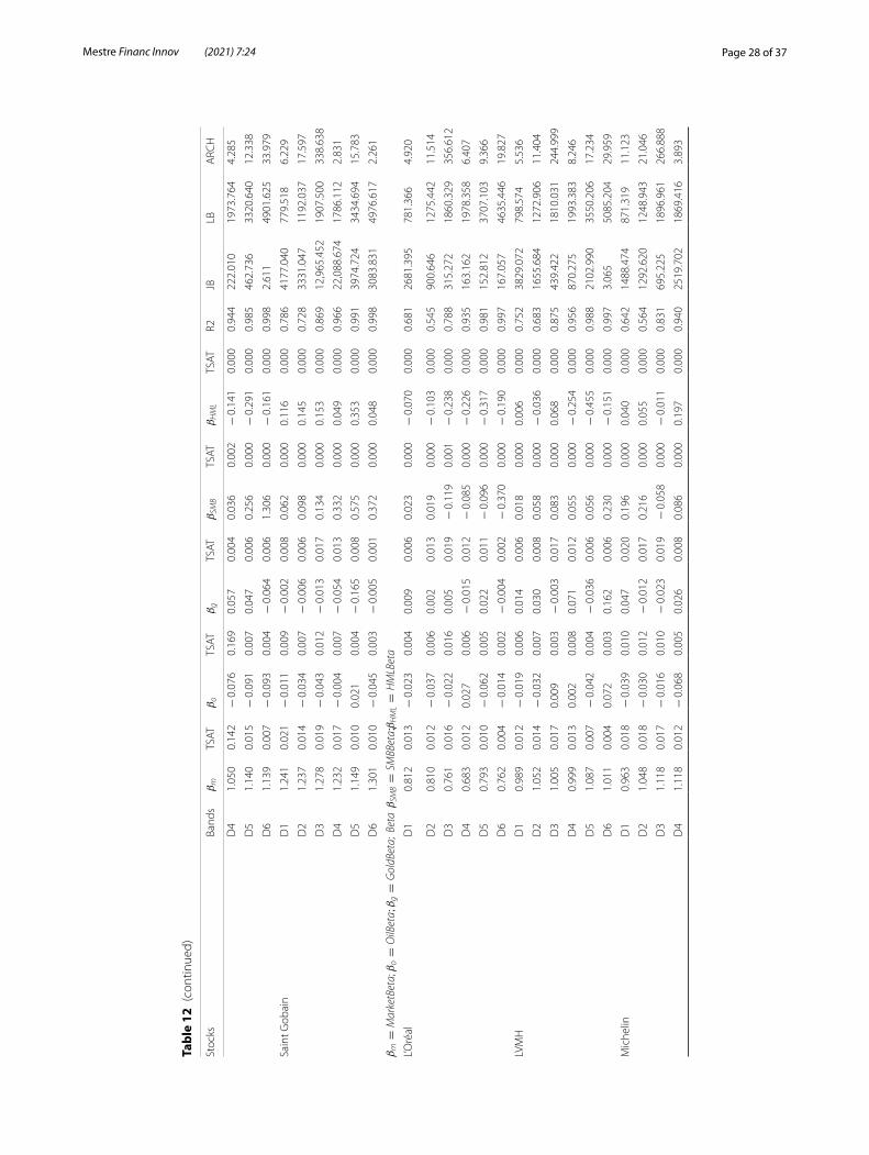
Page 28 of 37Mestre Financ Innov (2021) 7:24
Tabl
e 12
(co
ntin
ued)
Stoc
ksBa
nds
βm
TSAT
βo
TSAT
βg
TSAT
βSM
BTS
ATβHML
TSAT
R2JB
LBA
RCH
D4
1.05
00.
142
− 0
.076
0.16
90.
057
0.00
40.
036
0.00
2−
0.1
410.
000
0.94
422
2.01
019
73.7
644.
285
D5
1.14
00.
015
− 0
.091
0.00
70.
047
0.00
60.
256
0.00
0−
0.2
910.
000
0.98
546
2.73
633
20.6
4012
.338
D6
1.13
90.
007
− 0
.093
0.00
4−
0.0
640.
006
1.30
60.
000
− 0
.161
0.00
00.
998
2.61
149
01.6
2533
.979
Sain
t Gob
ain
D1
1.24
10.
021
− 0
.011
0.00
9−
0.0
020.
008
0.06
20.
000
0.11
60.
000
0.78
641
77.0
4077
9.51
86.
229
D2
1.23
70.
014
− 0
.034
0.00
7−
0.0
060.
006
0.09
80.
000
0.14
50.
000
0.72
833
31.0
4711
92.0
3717
.597
D3
1.27
80.
019
− 0
.043
0.01
2−
0.0
130.
017
0.13
40.
000
0.15
30.
000
0.86
912
,965
.452
1907
.500
338.
638
D4
1.23
20.
017
− 0
.004
0.00
7−
0.0
540.
013
0.33
20.
000
0.04
90.
000
0.96
622
,088
.674
1786
.112
2.83
1
D5
1.14
90.
010
0.02
10.
004
− 0
.165
0.00
80.
575
0.00
00.
353
0.00
00.
991
3974
.724
3434
.694
15.7
83
D6
1.30
10.
010
− 0
.045
0.00
3−
0.0
050.
001
0.37
20.
000
0.04
80.
000
0.99
830
83.8
3149
76.6
172.
261
βm=
MarketBeta
; βo=
OilBeta; β
g=
GoldBeta
; Beta
βSM
B=
SMBBeta;βHML=
HMLBeta
L’Oré
alD
10.
812
0.01
3−
0.0
230.
004
0.00
90.
006
0.02
30.
000
− 0
.070
0.00
00.
681
2681
.395
781.
366
4.92
0
D2
0.81
00.
012
− 0
.037
0.00
60.
002
0.01
30.
019
0.00
0−
0.1
030.
000
0.54
590
0.64
612
75.4
4211
.514
D3
0.76
10.
016
− 0
.022
0.01
60.
005
0.01
9−
0.1
190.
001
− 0
.238
0.00
00.
788
315.
272
1860
.329
356.
612
D4
0.68
30.
012
0.02
70.
006
− 0
.015
0.01
2−
0.0
850.
000
− 0
.226
0.00
00.
935
163.
162
1978
.358
6.40
7
D5
0.79
30.
010
− 0
.062
0.00
50.
022
0.01
1−
0.0
960.
000
− 0
.317
0.00
00.
981
152.
812
3707
.103
9.36
6
D6
0.76
20.
004
− 0
.014
0.00
2−
0.0
040.
002
− 0
.370
0.00
0−
0.1
900.
000
0.99
716
7.05
746
35.4
4619
.827
LVM
HD
10.
989
0.01
2−
0.0
190.
006
0.01
40.
006
0.01
80.
000
0.00
60.
000
0.75
238
29.0
7279
8.57
45.
536
D2
1.05
20.
014
− 0
.032
0.00
70.
030
0.00
80.
058
0.00
0−
0.0
360.
000
0.68
316
55.6
8412
72.9
0611
.404
D3
1.00
50.
017
0.00
90.
003
− 0
.003
0.01
70.
083
0.00
00.
068
0.00
00.
875
439.
422
1810
.031
244.
999
D4
0.99
90.
013
0.00
20.
008
0.07
10.
012
0.05
50.
000
− 0
.254
0.00
00.
956
870.
275
1993
.383
8.24
6
D5
1.08
70.
007
− 0
.042
0.00
4−
0.0
360.
006
0.05
60.
000
− 0
.455
0.00
00.
988
2102
.990
3550
.206
17.2
34
D6
1.01
10.
004
0.07
20.
003
0.16
20.
006
0.23
00.
000
− 0
.151
0.00
00.
997
3.06
550
85.2
0429
.959
Mic
helin
D1
0.96
30.
018
− 0
.039
0.01
00.
047
0.02
00.
196
0.00
00.
040
0.00
00.
642
1488
.474
871.
319
11.1
23
D2
1.04
80.
018
− 0
.030
0.01
2−
0.0
120.
017
0.21
60.
000
0.05
50.
000
0.56
412
92.6
2012
48.9
4321
.046
D3
1.11
80.
017
− 0
.016
0.01
0−
0.0
230.
019
− 0
.058
0.00
0−
0.0
110.
000
0.83
169
5.22
518
96.9
6126
6.88
8
D4
1.11
80.
012
− 0
.068
0.00
50.
026
0.00
80.
086
0.00
00.
197
0.00
00.
940
2519
.702
1869
.416
3.89
3
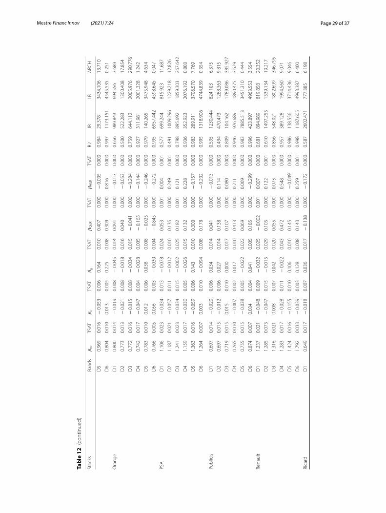
Page 29 of 37Mestre Financ Innov (2021) 7:24
Tabl
e 12
(co
ntin
ued)
Stoc
ksBa
nds
βm
TSAT
βo
TSAT
βg
TSAT
βSM
BTS
ATβHML
TSAT
R2JB
LBA
RCH
D5
0.96
90.
016
− 0
.053
0.00
60.
164
0.01
00.
407
0.00
0−
0.0
050.
000
0.98
429
.378
3434
.106
13.7
10
D6
0.80
40.
010
0.01
30.
005
0.22
50.
008
0.30
90.
000
0.81
60.
000
0.99
711
73.1
5145
45.5
350.
251
Ora
nge
D1
0.80
00.
014
− 0
.019
0.00
8−
0.0
450.
014
0.09
10.
000
− 0
.013
0.00
00.
656
989.
843
694.
556
3.68
9
D2
0.77
30.
013
− 0
.021
0.00
8−
0.0
180.
016
0.04
00.
000
− 0
.053
0.00
00.
500
522.
283
1300
.408
17.8
54
D3
0.77
20.
016
− 0
.015
0.00
8−
0.0
340.
015
− 0
.041
0.00
0−
0.2
040.
000
0.75
964
4.11
220
05.9
7629
0.77
6
D4
0.74
20.
017
− 0
.047
0.00
4−
0.0
280.
005
− 0
.163
0.00
0−
0.1
440.
000
0.92
731
1.98
120
01.3
281.
242
D5
0.78
30.
010
0.01
20.
006
0.03
80.
008
− 0
.023
0.00
0−
0.2
460.
000
0.97
914
0.26
534
75.9
484.
634
D6
0.76
60.
005
0.05
60.
003
− 0
.030
0.00
4−
0.8
450.
000
− 0
.272
0.00
00.
995
6957
.442
4598
.645
0.04
7
PSA
D1
1.10
60.
023
− 0
.034
0.01
3−
0.0
780.
024
0.05
30.
001
0.00
40.
001
0.57
769
9.24
481
5.92
311
.687
D2
1.18
70.
021
− 0
.057
0.01
1−
0.0
120.
010
0.13
50.
000
0.24
90.
001
0.49
110
09.2
9612
29.2
1812
.826
D3
1.24
10.
023
− 0
.034
0.01
5−
0.0
020.
025
0.18
20.
001
0.12
10.
000
0.79
889
5.69
218
59.3
0326
7.64
2
D4
1.15
90.
017
− 0
.030
0.00
5−
0.0
260.
015
0.13
20.
000
0.22
80.
000
0.93
635
2.92
320
76.1
920.
803
D5
1.36
30.
016
− 0
.059
0.00
60.
143
0.01
00.
300
0.00
0−
0.1
570.
000
0.98
328
9.91
137
06.5
707.
769
D6
1.26
40.
007
0.00
30.
010
− 0
.094
0.00
80.
178
0.00
0−
0.2
020.
000
0.99
513
18.9
0647
44.8
390.
354
Publ
icis
D1
0.69
70.
014
− 0
.020
0.00
60.
034
0.01
40.
041
0.00
0−
0.0
130.
000
0.59
512
30.4
4482
4.10
36.
375
D2
0.69
70.
015
− 0
.012
0.00
60.
027
0.01
40.
138
0.00
00.
114
0.00
00.
494
470.
473
1288
.363
9.81
5
D3
0.71
90.
015
0.01
50.
010
0.00
00.
017
0.10
70.
000
0.08
00.
000
0.80
910
4.16
217
89.0
8638
5.92
7
D4
0.76
50.
010
− 0
.007
0.00
20.
017
0.01
00.
413
0.00
00.
211
0.00
00.
946
976.
689
1890
.475
3.62
9
D5
0.75
50.
015
− 0
.038
0.00
5−
0.0
220.
022
0.06
90.
000
0.06
90.
000
0.98
378
85.5
1334
51.3
100.
444
D6
0.87
40.
007
0.03
40.
004
0.04
10.
005
0.18
50.
000
− 0
.299
0.00
00.
996
423.
897
4963
.553
3.55
4
Rena
ult
D1
1.23
70.
021
− 0
.048
0.00
9−
0.0
320.
025
− 0
.002
0.00
10.
007
0.00
00.
681
894.
989
819.
858
20.3
52
D2
1.28
50.
073
− 0
.047
0.01
5−
0.0
150.
029
0.10
50.
000
0.12
20.
001
0.61
014
97.2
5313
39.1
3419
.217
D3
1.31
60.
021
0.00
80.
007
0.04
20.
020
0.05
50.
000
0.07
30.
000
0.85
654
8.02
118
02.6
9934
6.79
5
D4
1.28
30.
017
− 0
.028
0.01
1−
0.0
220.
043
0.47
20.
000
0.54
80.
000
0.95
738
9.12
819
94.5
609.
071
D5
1.42
40.
016
− 0
.155
0.01
00.
106
0.01
00.
145
0.00
0−
0.0
490.
000
0.98
613
8.55
637
14.4
369.
046
D6
1.79
20.
033
− 0
.039
0.00
30.
128
0.00
80.
143
0.00
00.
259
0.00
10.
998
1187
.605
4993
.387
6.40
0
Rica
rdD
10.
649
0.01
7−
0.0
180.
007
0.03
60.
017
− 0
.138
0.00
0−
0.1
720.
000
0.58
726
02.4
7177
7.38
56.
198

Page 30 of 37Mestre Financ Innov (2021) 7:24
Tabl
e 12
(co
ntin
ued)
Stoc
ksBa
nds
βm
TSAT
βo
TSAT
βg
TSAT
βSM
BTS
ATβHML
TSAT
R2JB
LBA
RCH
D2
0.66
10.
014
− 0
.008
0.01
00.
016
0.01
7−
0.1
650.
000
− 0
.342
0.00
00.
460
1736
.476
1271
.797
23.0
78
D3
0.64
40.
014
− 0
.010
0.00
70.
093
0.01
2−
0.0
670.
000
− 0
.274
0.00
00.
766
8004
.109
1796
.284
352.
040
D4
0.73
10.
011
0.01
00.
004
− 0
.005
0.00
7−
0.0
270.
000
− 0
.414
0.00
00.
925
3030
.111
1834
.277
1.77
4
D5
0.70
00.
011
0.01
50.
004
0.00
50.
005
− 0
.113
0.00
0−
0.2
700.
000
0.98
196
3.25
035
28.9
4716
.162
D6
0.93
00.
005
− 0
.011
0.00
30.
061
0.00
3−
0.3
910.
000
− 0
.182
0.00
00.
997
2556
.860
4546
.120
2.09
0
βm=
MarketBeta
; βo=
OilBeta; β
g=
GoldBeta
; Beta
βSM
B=
SMBBeta;βHML=
HMLBeta
Schn
eide
rD
11.
246
0.01
6−
0.0
100.
007
− 0
.013
0.01
10.
034
0.00
00.
064
0.00
00.
804
319.
223
812.
444
6.15
8
D2
1.19
30.
015
− 0
.009
0.00
4−
0.0
150.
006
0.03
10.
000
0.15
00.
000
0.71
735
1.23
612
96.2
7014
.686
D3
1.16
30.
016
− 0
.025
0.00
90.
010
0.01
60.
167
0.00
00.
180
0.00
00.
863
485.
350
1921
.742
392.
911
D4
1.24
80.
025
− 0
.004
0.03
00.
068
0.01
60.
253
0.00
0−
0.1
530.
000
0.96
688
.112
2005
.775
10.4
28
D5
1.22
00.
009
− 0
.042
0.00
50.
043
0.00
90.
031
0.00
00.
096
0.00
00.
989
29.9
7736
45.9
525.
169
D6
1.10
80.
014
0.02
20.
003
0.13
80.
020
0.09
20.
000
− 0
.256
0.00
00.
997
5.18
453
62.5
1219
.295
Soci
été
Gén
éral
eD
11.
296
0.01
9−
0.0
020.
006
− 0
.075
0.01
2−
0.0
250.
000
0.18
60.
001
0.69
412
,141
.047
782.
822
5.84
9
D2
1.37
30.
019
− 0
.045
0.01
8−
0.1
160.
014
0.04
80.
001
0.34
40.
002
0.59
315
,146
.487
1242
.610
13.2
84
D3
1.31
20.
019
− 0
.043
0.00
6−
0.1
220.
014
− 0
.068
0.00
00.
332
0.00
00.
838
8283
.915
1969
.654
274.
576
D4
1.54
00.
014
− 0
.073
0.00
4−
0.1
820.
007
− 0
.336
0.00
00.
629
0.00
00.
957
4189
.733
1934
.230
2.01
5
D5
1.35
30.
010
− 0
.128
0.00
6−
0.0
930.
005
− 0
.322
0.00
00.
265
0.00
00.
986
1486
.861
3069
.794
2.13
0
D6
1.56
30.
012
− 0
.153
0.00
4−
0.1
090.
006
− 0
.002
0.00
0−
0.0
590.
000
0.99
843
76.9
4247
98.0
760.
051
Sode
xoD
10.
604
0.01
4−
0.0
200.
008
− 0
.006
0.01
5−
0.0
910.
000
− 0
.117
0.00
00.
567
2170
.828
779.
146
7.37
9
D2
0.63
50.
013
− 0
.008
0.00
90.
014
0.01
4−
0.1
000.
000
− 0
.171
0.00
00.
463
1521
.985
1229
.036
12.4
71
D3
0.51
40.
014
0.00
10.
008
− 0
.003
0.01
60.
074
0.00
0−
0.0
460.
000
0.75
660
8.41
718
35.9
3229
8.50
8
D4
0.62
80.
009
− 0
.021
0.00
40.
124
0.01
1−
0.0
470.
000
− 0
.091
0.00
00.
930
264.
991
2125
.131
3.39
4
D5
0.59
50.
011
− 0
.054
0.00
50.
122
0.01
00.
457
0.00
00.
095
0.00
00.
981
161.
283
3376
.248
10.8
78
D6
0.65
90.
005
0.04
30.
004
0.21
90.
008
− 0
.144
0.00
0−
0.0
760.
000
0.99
522
.967
4854
.986
14.7
04
Tech
nip
D1
0.88
20.
022
0.10
10.
011
0.11
90.
027
0.08
80.
000
0.28
80.
000
0.61
623
49.7
4382
4.45
64.
035
D2
0.90
80.
021
0.14
20.
012
0.08
10.
019
0.08
80.
000
0.10
50.
000
0.49
410
23.3
5712
79.8
9219
.541
D3
0.93
70.
023
0.19
80.
015
0.02
70.
027
0.20
00.
001
0.23
70.
001
0.79
720
11.7
9318
98.2
8939
8.72
2
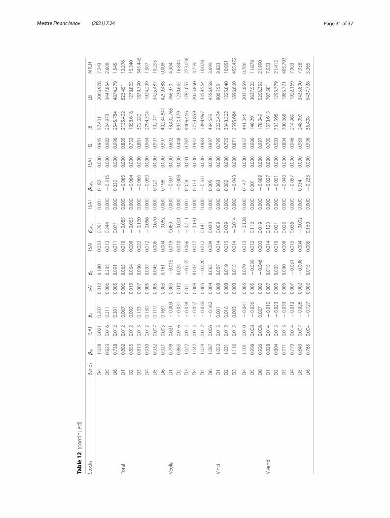
Page 31 of 37Mestre Financ Innov (2021) 7:24
Tabl
e 12
(co
ntin
ued)
Stoc
ksBa
nds
βm
TSAT
βo
TSAT
βg
TSAT
βSM
BTS
ATβHML
TSAT
R2JB
LBA
RCH
D4
1.02
80.
021
0.20
70.
012
0.18
00.
033
0.29
10.
001
0.18
20.
000
0.94
557
.401
2066
.978
7.24
3
D5
0.92
30.
016
0.21
10.
006
0.23
50.
013
0.24
40.
000
− 0
.315
0.00
00.
982
224.
973
3447
.854
2.60
8
D6
0.73
80.
012
0.30
10.
005
0.09
10.
011
0.07
10.
000
0.23
00.
000
0.99
625
45.7
8448
74.2
791.
545
Tota
lD
10.
882
0.01
20.
067
0.00
60.
065
0.01
0−
0.0
850.
000
− 0
.065
0.00
00.
805
2135
.402
823.
451
13.2
76
D2
0.85
50.
012
0.09
20.
015
0.06
40.
009
− 0
.063
0.00
0−
0.0
640.
000
0.73
210
58.6
1612
78.8
2315
.340
D3
0.81
30.
013
0.13
30.
007
0.03
60.
022
− 0
.160
0.00
0−
0.0
660.
000
0.88
137
2.02
018
79.7
9034
5.44
6
D4
0.93
00.
012
0.13
00.
005
0.03
70.
012
− 0
.056
0.00
0−
0.0
500.
000
0.96
427
94.3
0419
24.2
991.
507
D5
0.93
20.
007
0.11
90.
005
0.04
50.
005
− 0
.070
0.00
00.
020
0.00
00.
991
102.
071
3425
.487
10.2
95
D6
0.92
10.
005
0.16
90.
003
0.16
10.
004
− 0
.062
0.00
00.
198
0.00
00.
997
40,2
34.8
4142
99.4
880.
008
Veol
iaD
10.
799
0.02
1−
0.0
030.
009
− 0
.015
0.01
90.
080
0.00
0−
0.0
310.
000
0.60
218
,492
.765
766.
970
4.30
4
D2
0.86
50.
016
− 0
.031
0.01
00.
024
0.01
0−
0.0
010.
000
− 0
.008
0.00
00.
448
8070
.179
1230
.665
16.8
44
D3
1.02
20.
015
− 0
.038
0.02
1−
0.0
550.
066
− 0
.211
0.00
10.
029
0.00
10.
787
9409
.466
1781
.057
273.
058
D4
1.04
20.
013
− 0
.057
0.00
80.
007
0.01
7−
0.1
810.
000
0.03
30.
000
0.94
227
34.8
5920
25.8
503.
759
D5
1.02
40.
012
− 0
.039
0.00
5−
0.0
200.
012
0.14
10.
000
− 0
.331
0.00
00.
983
1394
.997
3359
.564
10.0
78
D6
1.08
70.
006
− 0
.162
0.00
40.
063
0.00
40.
030
0.00
00.
005
0.00
00.
997
434.
629
4556
.958
3.69
9
Vinc
iD
11.
053
0.01
30.
001
0.00
80.
007
0.01
40.
009
0.00
00.
063
0.00
00.
795
2220
.474
806.
155
9.82
3
D2
1.03
10.
012
0.01
60.
008
0.01
90.
015
0.03
90.
000
0.08
20.
000
0.72
533
43.3
0212
25.8
4010
.051
D3
1.11
60.
015
0.00
30.
008
0.01
50.
014
− 0
.014
0.00
0−
0.0
430.
000
0.87
125
95.6
8418
96.6
6045
5.47
2
D4
1.10
10.
010
− 0
.041
0.00
50.
079
0.01
3−
0.1
280.
000
0.14
70.
000
0.95
744
1.04
620
31.8
590.
706
D5
0.99
80.
008
− 0
.036
0.00
5−
0.0
390.
012
0.11
20.
000
0.00
10.
000
0.98
614
6.29
136
37.5
2311
.878
D6
0.92
60.
006
0.02
70.
002
− 0
.046
0.00
30.
019
0.00
0−
0.0
090.
000
0.99
717
8.04
952
06.3
5321
.990
Vive
ndi
D1
0.82
80.
014
− 0
.010
0.00
70.
015
0.01
40.
123
0.00
0−
0.0
270.
000
0.70
515
73.6
1579
7.58
17.
533
D2
0.80
40.
013
− 0
.023
0.00
50.
003
0.01
00.
021
0.00
0−
0.0
510.
000
0.58
373
3.59
812
95.7
7921
.415
D3
0.77
10.
013
− 0
.033
0.00
50.
030
0.00
90.
022
0.00
0−
0.0
400.
000
0.80
470
0.66
819
85.7
7140
5.79
3
D4
0.77
90.
014
− 0
.012
0.00
7−
0.0
510.
015
0.03
60.
000
− 0
.057
0.00
00.
946
214.
969
1922
.169
7.90
3
D5
0.84
00.
007
− 0
.026
0.00
2−
0.0
980.
004
− 0
.002
0.00
00.
034
0.00
00.
983
248.
090
3435
.890
7.93
8
D6
0.76
50.
004
− 0
.127
0.00
20.
015
0.00
50.
160
0.00
0−
0.2
330.
000
0.99
636
.408
5437
.728
5.36
5
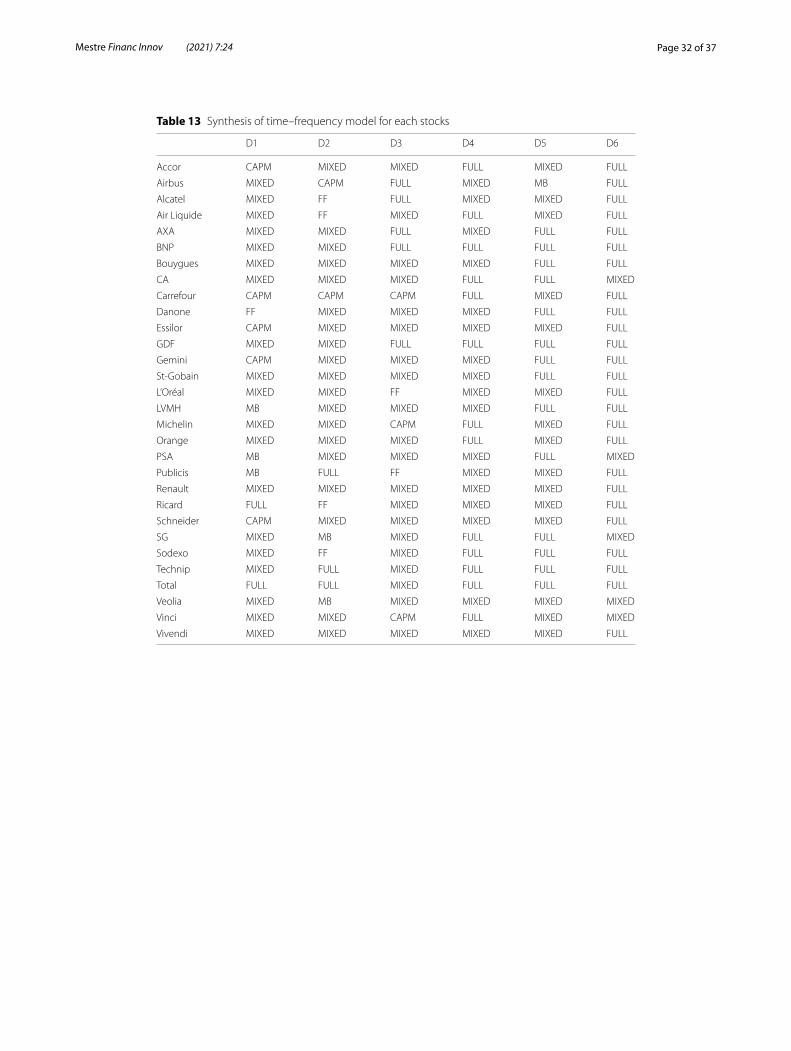
Page 32 of 37Mestre Financ Innov (2021) 7:24
Table 13 Synthesis of time–frequency model for each stocks
D1 D2 D3 D4 D5 D6
Accor CAPM MIXED MIXED FULL MIXED FULL
Airbus MIXED CAPM FULL MIXED MB FULL
Alcatel MIXED FF FULL MIXED MIXED FULL
Air Liquide MIXED FF MIXED FULL MIXED FULL
AXA MIXED MIXED FULL MIXED FULL FULL
BNP MIXED MIXED FULL FULL FULL FULL
Bouygues MIXED MIXED MIXED MIXED FULL FULL
CA MIXED MIXED MIXED FULL FULL MIXED
Carrefour CAPM CAPM CAPM FULL MIXED FULL
Danone FF MIXED MIXED MIXED FULL FULL
Essilor CAPM MIXED MIXED MIXED MIXED FULL
GDF MIXED MIXED FULL FULL FULL FULL
Gemini CAPM MIXED MIXED MIXED FULL FULL
St-Gobain MIXED MIXED MIXED MIXED FULL FULL
L’Oréal MIXED MIXED FF MIXED MIXED FULL
LVMH MB MIXED MIXED MIXED FULL FULL
Michelin MIXED MIXED CAPM FULL MIXED FULL
Orange MIXED MIXED MIXED FULL MIXED FULL
PSA MB MIXED MIXED MIXED FULL MIXED
Publicis MB FULL FF MIXED MIXED FULL
Renault MIXED MIXED MIXED MIXED MIXED FULL
Ricard FULL FF MIXED MIXED MIXED FULL
Schneider CAPM MIXED MIXED MIXED MIXED FULL
SG MIXED MB MIXED FULL FULL MIXED
Sodexo MIXED FF MIXED FULL FULL FULL
Technip MIXED FULL MIXED FULL FULL FULL
Total FULL FULL MIXED FULL FULL FULL
Veolia MIXED MB MIXED MIXED MIXED MIXED
Vinci MIXED MIXED CAPM FULL MIXED MIXED
Vivendi MIXED MIXED MIXED MIXED MIXED FULL
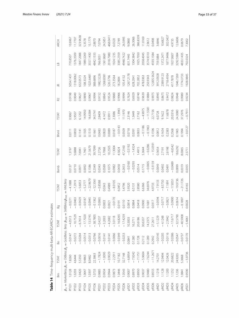
Page 33 of 37Mestre Financ Innov (2021) 7:24
Tabl
e 14
Tim
e–fre
quen
cy m
ulti-
beta
-AR-
EGA
RCH
est
imat
es
BmTS
TAT
BoTS
TAT
BgTS
TAT
Bsm
bTS
TAT
Bhm
lTS
TAT
R2JB
LBA
RCH
βm=
MarketBeta
; βo=
OilBeta; β
g=
GoldBeta
; Beta
βSM
B=
SMBBeta;βHML=
HMLBeta
Pf1D
11.
0128
1.82
60−
0.0
147
− 4
.051
3−
0.0
271
− 4
.188
80.
0137
1.31
970.
0111
0.90
670.
9198
5054
.143
177
0.85
0710
.696
7
Pf1D
21.
0293
4.64
44−
0.0
272
− 1
0.75
29−
0.0
463
− 7
.291
90.
0710
5.68
880.
0850
5.95
070.
9049
1318
.006
213
76.3
509
11.7
707
Pf1D
31.
0420
5.53
50−
0.0
264
− 6
.761
4−
0.0
429
− 5
.605
30.
0971
7.69
410.
1141
6.12
020.
9627
632.
0573
1847
.208
832
3.96
38
Pf1D
41.
0647
9.48
63−
0.0
514
− 1
7.70
20−
0.0
187
− 5
.277
70.
0092
1.74
010.
1505
14.9
950
0.98
9010
8.33
2419
89.3
269
5.35
78
Pf1D
51.
0397
8.04
82−
0.0
313
− 1
3.57
45−
0.0
945
− 2
2.96
790.
1586
21.5
679
0.15
1016
.638
40.
9967
1025
.648
135
57.1
430
15.1
779
Pf1D
61.
0733
22.3
863
− 0
.076
6−
38.
7805
− 0
.136
2−
52.
3561
0.23
4939
.709
90.
1661
34.5
741
0.99
9438
8.68
9648
42.1
533
2.88
70
Pf2D
10.
9885
− 1
.782
4−
0.0
016
− 0
.423
7−
0.0
065
− 0
.858
80.
0343
2.27
260.
0483
2.84
090.
9152
1982
.322
676
6.00
517.
0794
Pf2D
20.
9934
− 1
.009
5−
0.0
141
− 3
.200
30.
0003
0.03
430.
0589
3.70
680.
0820
4.14
720.
8843
1268
.838
113
61.8
681
24.5
851
Pf2D
30.
9944
− 0
.902
9−
0.0
141
− 4
.268
20.
0021
0.49
890.
1075
10.2
505
0.00
890.
9911
0.95
2452
6.57
9620
18.7
980
468.
0411
Pf2D
40.
9873
− 2
.291
1−
0.0
066
− 3
.011
8−
0.0
170
− 8
.010
50.
0982
11.3
004
0.01
872.
3086
0.98
8027
3.35
6419
24.1
235
6.03
20
Pf2D
51.
0446
10.7
182
− 0
.034
9−
16.
8265
0.01
916.
0452
0.04
304.
5824
− 0
.014
3−
1.3
943
0.99
6618
.280
433
85.2
359
7.27
49
Pf2D
61.
0543
32.7
148
− 0
.025
3−
17.
4259
0.01
105.
4796
0.26
5347
.216
00.
0509
11.1
970
0.99
9410
5.41
3249
48.7
422
26.5
995
pf3D
10.
9007
− 6
.895
40.
0841
10.3
003
0.08
145.
9320
− 0
.016
0−
0.5
192
0.07
182.
3146
0.76
2412
67.2
178
831.
7440
9.08
60
pf3D
20.
8970
− 7
.924
20.
1280
16.2
711
0.08
646.
5131
− 0
.029
3−
1.4
324
0.03
911.
3449
0.69
2962
8.20
4113
04.3
842
26.3
066
pf3D
30.
8950
− 7
.175
10.
1728
20.6
186
0.04
182.
8580
0.05
141.
4915
0.08
332.
7162
0.87
4070
2.28
5219
25.7
050
386.
8339
pf3D
40.
9037
− 5
.960
40.
2112
30.6
337
0.09
006.
6366
0.17
155.
3644
− 0
.118
6−
4.9
075
0.96
3947
8.03
6320
58.4
045
11.0
169
pf3D
50.
9480
− 7
.624
40.
1289
14.2
375
0.16
8134
.697
6−
0.0
005
− 0
.028
6−
0.1
963
− 1
1.55
810.
9884
250.
9343
3574
.931
02.
9612
pf3D
60.
8555
− 1
1.26
710.
2942
27.2
611
0.03
174.
9733
− 0
.315
9−
15.
0591
0.15
9622
.715
60.
9975
12,0
05.5
624
4593
.158
40.
0498
pf4D
11.
1218
14.2
701
− 0
.014
5−
5.1
229
− 0
.059
4−
7.9
133
0.00
490.
3654
0.08
126.
0728
0.89
4539
12.0
928
759.
5884
3.68
46
pf4D
21.
1128
12.9
494
− 0
.020
5−
4.1
248
− 0
.071
7−
8.5
750
0.04
922.
7191
0.16
349.
1622
0.86
7523
89.9
123
1372
.247
110
.682
7
pf4D
31.
1200
12.0
426
− 0
.011
6−
2.3
942
− 0
.082
1−
7.1
891
0.04
912.
6198
0.23
8311
.687
80.
9472
2718
.493
418
77.9
496
302.
0437
pf4D
41.
1252
20.6
822
− 0
.038
6−
17.
6717
− 0
.090
0−
17.
8351
− 0
.048
9−
4.6
542
0.25
6820
.031
60.
9824
417.
7878
1927
.060
74.
9735
pf4D
51.
1236
24.9
265
− 0
.054
7−
32.
5790
− 0
.061
4−
19.
0736
0.08
9918
.629
20.
1965
24.3
080
0.99
4810
46.7
269
3292
.598
412
.660
6
pf4D
61.
0841
5.36
68−
0.0
737
− 4
0.59
08−
0.1
897
− 2
1.17
260.
0319
8.00
650.
1994
37.2
976
0.99
8917
74.3
733
4833
.143
50.
0679
pf5D
10.
9590
− 5
.973
6−
0.0
170
− 5
.406
10.
0028
0.41
650.
0355
2.57
11−
0.0
127
− 0
.791
10.
9234
1928
.984
579
2.03
247.
3002
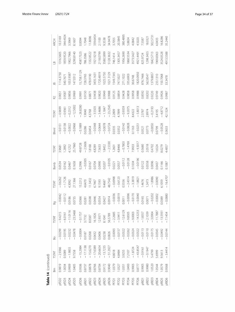
Page 34 of 37Mestre Financ Innov (2021) 7:24
Tabl
e 14
(co
ntin
ued)
BmTS
TAT
BoTS
TAT
BgTS
TAT
Bsm
bTS
TAT
Bhm
lTS
TAT
R2JB
LBA
RCH
pf5D
20.
9819
− 2
.936
6−
0.0
299
− 9
.421
5−
0.0
042
− 0
.626
20.
0534
3.96
81−
0.0
151
− 0
.969
90.
9051
1114
.373
013
16.5
605
10.3
169
pf5D
31.
0034
0.50
89−
0.0
195
− 6
.016
1−
0.0
112
− 1
.712
60.
0162
1.28
92−
0.0
138
− 0
.936
10.
9587
540.
7671
1859
.952
034
4.49
24
pf5D
40.
9909
− 1
.985
5−
0.0
232
− 1
1.01
160.
0186
4.30
920.
0467
4.12
52−
0.0
022
− 0
.231
20.
9856
1053
.938
719
02.7
966
3.39
69
pf5D
51.
0405
9.75
58−
0.0
478
− 2
3.54
680.
0735
27.1
366
0.16
5825
.796
0−
0.0
968
− 1
2.50
020.
9969
147.
0312
3290
.814
08.
1607
pf5D
60.
9506
− 1
5.29
84−
0.0
004
− 0
.175
70.
0366
15.2
212
0.29
9649
.872
8−
0.1
889
− 2
6.82
800.
9991
15,7
58.1
129
4587
.752
30.
0094
pf6D
10.
8737
− 1
7.11
380.
0187
3.77
320.
0281
4.64
70−
0.0
305
− 2
.560
60.
0286
1.90
400.
9150
728.
3765
786.
3586
1.70
48
pf6D
20.
8878
− 1
5.62
700.
0268
8.05
870.
0598
11.5
432
0.01
671.
8168
0.04
544.
3768
0.88
7147
8.91
9013
32.8
522
11.8
096
pf6D
30.
8766
− 1
7.63
890.
0432
16.1
826
0.04
466.
7467
0.07
044.
8289
− 0
.034
8−
3.5
503
0.94
3834
35.1
631
1921
.921
833
9.64
54
pf6D
40.
8704
− 2
0.66
540.
0406
12.9
371
0.05
549.
1593
0.09
907.
5633
− 0
.064
4−
3.4
686
0.98
2017
20.4
819
2118
.079
92.
1100
pf6D
50.
9172
− 1
3.72
350.
0238
8.10
410.
0427
9.46
870.
0207
1.84
52−
0.0
078
− 1
.184
70.
9949
1025
.575
035
80.5
899
9.35
38
pf6D
60.
9040
− 5
1.29
270.
0826
56.5
789
0.09
1448
.754
2−
0.0
105
− 2
.533
0−
0.0
724
− 2
3.25
450.
9988
1021
.312
951
28.3
632
34.9
478
Pf7D
11.
0379
4.80
18−
0.0
093
− 2
.268
5−
0.0
036
− 0
.699
80.
0221
1.26
010.
0335
2.28
090.
9125
1549
.734
574
6.14
143.
7055
Pf7D
21.
0327
4.84
84−
0.0
157
− 3
.941
1−
0.0
019
− 0
.612
30.
0557
4.84
660.
0352
4.78
990.
8854
747.
5027
1305
.345
720
.384
5
Pf7D
31.
0351
3.92
55−
0.0
322
− 1
2.61
290.
0011
0.55
56−
0.0
112
− 0
.780
3−
0.0
142
− 0
.935
90.
9428
271.
1022
1956
.269
038
0.48
95
Pf7D
41.
0493
7.21
07−
0.0
262
− 9
.850
5−
0.0
096
− 2
.431
4−
0.0
128
− 1
.476
9−
0.0
828
− 9
.207
50.
9858
335.
6903
1860
.553
45.
8824
Pf7D
50.
9905
− 1
.872
4−
0.0
324
− 9
.000
3−
0.0
170
− 3
.381
90.
1034
7.99
330.
1163
8.43
220.
9958
30.6
748
3573
.542
74.
0842
Pf7D
60.
8777
− 4
3.85
47−
0.0
322
− 1
4.32
53−
0.0
040
− 1
.882
1−
0.0
196
− 9
.301
7−
0.0
251
− 5
.801
30.
9988
1820
.095
049
21.4
491
4.50
20
pf8D
10.
9905
− 0
.916
1−
0.0
113
− 1
.835
70.
0165
1.46
760.
0122
0.56
800.
0521
2.37
870.
8592
876.
7466
825.
9724
7.55
87
pf8D
20.
9980
− 0
.194
7−
0.0
110
− 2
.103
90.
0071
1.24
730.
0558
2.05
180.
0773
2.89
740.
8202
562.
8547
1298
.345
518
.032
1
pf8D
31.
0520
5.47
99−
0.0
175
− 3
.090
4−
0.0
202
− 1
.898
60.
0096
0.47
02−
0.00
50−
0.2
193
0.92
2013
79.8
857
1842
.571
330
2.57
31
pf8D
41.
0544
5.69
99−
0.0
545
− 1
1.78
87−
0.0
002
− 0
.009
00.
0437
1.63
240.
0799
3.41
950.
9749
233.
1310
1969
.836
34.
0433
pf8D
51.
0579
9.56
13−
0.0
492
− 1
3.59
310.
0389
6.10
590.
1166
8.02
79−
0.0
528
− 4
.871
20.
9926
150.
7068
3524
.052
816
.828
6
pf8D
60.
9568
− 3
.441
4−
0.0
144
− 7
.145
4−
0.0
880
− 1
6.47
070.
1087
4.48
570.
3633
42.1
324
0.99
8733
.347
849
13.5
588
35.2
440
Page 35 of 37Mestre Financ Innov (2021) 7:24
AbbreviationsCAPM: Capital Assets Pricing Model; SML: Securities Market Line; APT: Arbitrage Pricing Theory; MB: Multi-Beta (referring to Multi-Beta Model; TFMB: Time–Frequency Multi-Betas Model; OLS: Ordinary Least Squares; TSTAT : Student Statistic; BLUE: Best Linear Unbiased Estimator; JB: Jarque–Bera; LB: Ljung-Box; ARCH: AutoRegressive Conditional Heteroskedastic-ity; ARMA: Auto Regressive Moving Average; E/GARCH: Exponential/Generalised AutoRegressive Conditional Heteroske-dasticity; DCC-GARCH: Dynamic Conditional Correlation Generalised AutoRegressive Conditional Heteroskedasticity; BEKK-GARCH: Baba Engle Kraft Kroner Generalised AutoRegressive Conditional Heteroskedasticity; CAC40: Cotations Assistées Continues 40 (main index of Bourse de Paris); OAT: Obligation Assimilable du Trésor (French Treasury Bonds Rate); HFT: High-Frequency Trader; MODWT: Maximal Overlap Discrete Wavelets Transform; GDF: Gaz de France; LVMH: Louis Vuitton Moet Hennessy; PSA: Peugeot Société Anonyme; BNP: Banque Nationale de Paris-Paribas; SG: Société Générale; CA: Crédit Agricole.
AcknowledgementsNot applicable.
Authors’ contributionsAs unique author, RM fully analyse, compute, write and approved the final manuscript. RM is the corresponding author. The author read and approved the final manuscript.
FundingThis research received no specific grant from any funding agency in the public, commercial, or not-for-profit sectors.
Availability of data and materialsThe datasets used and analysed during the current study are available from the corresponding author on reasonable request. In others, data are free available on any data providers. For Fama–French Factors data ara available on French website: https:// mba. tuck. dartm outh. edu/ pages/ facul ty/ ken. french/ data_ libra ry. html.
Declarations
Competing interestsThe authors declare that they have no competing interests.
Received: 6 July 2020 Accepted: 25 March 2021
ReferencesAguiar-Conraria L, Soares MJ (2014) The continuous Wavelet Transorm: moving beyond uni and bivariate analysis. J Econ
Surv 28(2):344–375Arfaoui M, Ben Rejeb A (2017) Oil, gold, US dollar and stock market interdependencies: a global analytical insight. Eur J
Manag Bus Econ 26(3):278–293. https:// doi. org/ 10. 1108/ EJMBE- 10- 2017- 016Bantz R (1981) The relationship between return and market value of common stocks. J Financ Econ 9(1):3–18Basher SA, Sadorsky P (2006) Oil price risk and emerging stock markets. Glob Financ J 17(2):224–251Basu S (1983) The relationship between earnings yield, market value and return for NYSE common stocks: further evi-
dence. J Financ Econ 12(1):129–156Baur DG, Lucey B (2010) Is gold a hedge or a safe haven? An analysis of stocks, bonds and gold. Financ Rev 45(2):217–229Baur DG, McDermott TK (2010) Is gold a safe haven? International evidence. J Bank Finance 34:1886–1898Baur DG, McDermott TKJ (2016) Why is gold a safe haven? J Behav Exp Financ 10:63–71Bendod A, Chikhi M, Bennaceur F (2017) Testing the CAPM-GARCH MODELS in the GCC-wide equity sectors. Asian J Econ
Model 5(4):413–430Bera A, Bubnys E, Park H (1988) Conditional heteroscedasticity in the market model and efficient estimates of betas.
Financ Rev 23(2):201–214Black F, Jensen M, Scholes M (1972) The capital asset pricing model: some empirical test; studies in the theory of capital
markets edited by M. Jensen. Praeger Publishers, New YorkBollerslev T (1986) Genealized autoregressive conditionnal heteroskedasticity. J Econ 31:307–327Bollerslev T, Engle R, Wooldridge H (1988) A Capital asset pricing model with time-varying covariance. J Polit Econ
96(1):116–131Bos T, Newbold P (1984) An empirical investigation of the possibility of stochastic systematic risk in the market model. J
Bus 57(1):37–47Boyer MM, Filion D (2007) Common and fundamental factors instock returns of Canadian oil and gas companies. Energy
Econ 29(3):428–453Brooks RD, Faff RW, McKenzie MD (1998) Time-varying beta risk of Australian industry portfolios: a comparison of model-
ling techniques. Aust J Manag 23(1):1–22Chen NF, Roll R, Ross SA (1986) Economic forces and the stock market. J Bus 59(3):383–403Choudry T, Wu H (2008) Forecasting ability of GARCH vs Kalman filter method evidence from daily UK time-varying beta.
J Forecast 27:670–689Chua JH, Sick G, Woodward RS (1990) Diversifying with gold stocks. Financ Anal J 46:76–79Corhay A, Rad A (1996) Conditional heteroscedasticity adjusted market model and an event study. Q Rev Econ Finance
36(4):529–538
Page 36 of 37Mestre Financ Innov (2021) 7:24
Diebold F, Jang I, Jevons L (1988) Conditional heteroskedasticity in the market, finance and economics discussion series, 42, Division of Research and Statistics, Federal Reserve Board, Washington
Engle R (1982) Autoregressive conditional heteroskedasticity with estimates of the variance of UK inflation. Econometrica 50:987–1008
Engle R (2016) Dynamic conditional beta. J Financ Economet 14(4):643–667Fabozzi F, Francis J-C (1978) Beta as a random coefficient. J Financ Quant Anal 13(1):101–116Faff RW, Hiller D, Hiller J (2000) Time varying beta risk: an analysis of alternative modelling techniques. J Bus Financ Acc
27(2):523–555Fama E (1996) Multifactor portfolio efficiency and multifactor asset pricing. J Financ Quant Anal 31(4):441–465Fama E, French K (1992) Common risk factors in the returns on stocks and bonds. J Financ Econ 33(1):3–56Fama E, French KR (1996) The CAPM is wanted, dead or alive. J Finance 51(5):1947–1958Fama E, MacBeth J (1973) Risk, return, and equilibrium: empirical tests. J Polit Econ 81(3):607–636Fisher TJ, Gallagher C (2012) New weighted portmanteau statistics for time series goodness of fit testing. J Am Stat Assoc
107(498):777–787Gaffeo E (2019) Leverage and evolving heterogeneous beliefs in a simple agents-based financial market. Financ Res Lett
29:272–279Gençay R, Selçuk F, Whitcher B (2005) Systematic risk and timescales. Quant Finance 3(2):108–116Ghalanos A, Theussl S (2011) Rsolnp: general non-linear optimization using augmented Lagrange multiplier method, 1.11
editionGiaccoto C, Ali MM (1982) Optimal distribution free tests and further evidence of heteroskedasticity in the market model.
J Finance 37:1247–1257Groenewold N, Fraser P (1997) Share prices and macroeconomics factors. J Bus Financ Acc 24(9):1367–1384Groenewold N, Fraser P (1999) Time varying estimates of CAPM betas. Math Comput Simul 48:531–539He Z, O’Connor F, Thijssen J (2018) Is gold a sometime safe haven or an always hedge for equity investor? A Markov
switching CAPM approach for US and Uh stocks indices. Int Rev Financ Anal 60:30–37Heyman D, Lescrauwaet M, Stieperaere H (2019) Finance Res Lett 29:1–6Huang RD, Masulis RW, Stoll HR (1996) Energy shocks and financial markets. J Futur Mark 16(1):1–27HussainShahzad SJ, Raza N, Shahbaz M, Ali A (2017) Dependence of stock market with gold and bonds under bullish and
bearish Market States. Resour Policy 52(C):308–319Johnson M, Lamdin D (2015) New evidence on whether gold mining stock are more like gold or like stocks. Altern Invest
Anal Rev 5(2):31–38Jones DW, Leiby P, Paik I (2004) Oil price shocks and the macroeconomy: what has been learned since 1996. Energy J
25(2):1–32Kahraman E, Unal G (2019) Multiple wavelet coherency analysis and forecasting of metal prices. Financ Innov 5(22)Kou G, Peng Y, Wang G (2014) Evaluation of clustering algorithms for financial risk analysis using MCDM methods. Inf Sci
275:1–12Kou G, Xu Y, Peng Y, Shen F, Chen Y, Chang K, Kou S (2021) Bankruptcy prediction for SMEs using transactional data and
two-stage multi-objective feature selection. Decis Support Syst 140Lee CC, Zeng JH (2011) The impact of oil price shocks on stock market activities: asymetric effect with quantile regres-
sion. Math Comput Simul 81(7):1910–1920Lintner J (1965) The valuation of risk assets and the selection of risky investments in stock portfolios and capital budgets.
Rev Econ Stat 47(1):13–37Lintner J (1981) Some new perspectives on tests of CAPM and other capital asset pricing models and issues of market
efficiency; edited by Harvard Institute of Economic Research, discussion paperMallat S (1989) A theory for multiresolution signal decomposition: the wavelet representation. IEEE Trans Pattern Anal
Mach Intell 11(7)Mallat S (2001) Une exploration des signaux en ondelettes. Ecole polytechniqueMallat S (2009) Wavelet tour of signal processing: the sparse way. Academic PressMarkowitz H (1952) Portfolio selection. J Finance 7(1):77–91Merton RC (1973) Theory of rational option pricing. Bell J Econ Manag Sci 4(1):141–183Mestre R, Terraza M (2018) Time-frequency analysis of the CAPM—application to the CAC 40. Manag Glob Transit Int Res
J 16–2:141–157Mestre R, Terraza M (2020) Adjusted beta based on an empirical comparsion of OLS CAPM and the CAPM with EGARCH
errors. Int J Financ Econ. https:// doi. org/ 10. 1002/ ijfe. 1977Meyer Y (1990) Ondelettes et algorithmes concurrents. Actualités mathématiques Hermans éditions des sciences et des
arts xii: 217–381Mishra PK, Das JR, Mishra SK (2010) Gold price volatility and stock market returns in India. Am J Sci Res 9:49–55Miyazaki T, Toyoshima Y, Hamori S (2012) Exploring the dynamic interdependence between gold and other financial
markets. Econ Bull AccessEcon 32(1):37–50Morelli D (2003) Capital asset pricing models on UK securities using ARCH. Appl Financ Econ 13(3):211–223Mossin J (1966) Equilibrium in a capital asset market. Econometrica 34:768–783Nanayakkara N, Nimal PD, Weerakoo YK (2019) Behavioural asset pricing a review. Int J Econ Financ Issues 9(4):101–108Nasiri M, Nourollahzadeh N, Sarraf F, Hamidian M (2019) Modeling assets pricing using behavioral patterns Fama-French
approach. Iran J Finance 3(3):35–60Nelson D (1991) Conditional heteroskedasticity in asset return a new approach. Econometrica 59(2):347–370Ross S (1976) The arbitrage theory of capital pricing. J Econ Theory 13:341–360Schwert G, Seguin P (1990) Heteroscedasticity in stock returns. J Finance 45(4):1129–1155Sharpe W (1964) Capital asset prices: a theory of market equilibrium under risk. J Finance 19(3):425–442Sumner S, Johnson R, Soenen L (2010) Spillover effects between gold, stocks, and bonds. J Cent Cathedra 3(2):106–120Tsay H-J, Chen M-C, Yang C-Y (2014) A time-varying perspective on the CAPM and downside betas. Int Rev Econ Financ
29:440–454

Page 37 of 37Mestre Financ Innov (2021) 7:24
Tufano P (1998) The determinants of stock price exposure: Financial engineering and the gold mining industry. J Finance 53(3):1015–1052
Tuyon J, Ahmad Z (2018) Behavioural asset pricing determinants in a factor and style investing framework. Cap Mark Rev 26(2):32–52
Wen F, Xu L, Ouyang G, Kou G (2019) Retail investor attention and stock price crash risk: evidence from China. Int Rev Financ Anal 65:101376
Ye Y (1997) Interior point algorithms: theory and analysis. WileyYeo J (2001) Modelling time-varying systematic risk in Australia. In: Ghessemi M, McAleer L, Oxley MS (eds) Proceedings
of the international congress on modelling & simulation, vol 3, Canberra. ed. Western Australia: Modelling and Simulation Society of Australia and New Zealand Inc., pp 1565–1570
Publisher’s NoteSpringer Nature remains neutral with regard to jurisdictional claims in published maps and institutional affiliations.