A Vortex Particle Method for Two-Dimensional Compressible Flow · His method avoids computing the density gradient in the external force term by tracking this quantity directly rather

Journal of Computational Physics 179, 371–399 (2002)doi:10.1006/jcph.2002.7060

A Vortex Particle Method for Two-DimensionalCompressible Flow

Jeff D. Eldredge,1 Tim Colonius, and Anthony Leonard

Division of Engineering and Applied Science, California Institute of Technology, Pasadena, California 91125E-mail: [email protected], [email protected], and [email protected]

Received April 26, 2001; revised March 5, 2002

A vortex particle method is developed for simulating two-dimensional, unsteadycompressible flow. The method uses the Helmholtz decomposition of the velocityfield to separately treat the irrotational and solenoidal portions of the flow, and the par-ticles are allowed to change volume to conserve mass. In addition to having vorticityand dilatation properties, the particles also carry density, enthalpy, and entropy. Theresulting evolution equations contain terms that are computed with techniques usedin some incompressible methods. Truncation of unbounded domains via a nonre-flecting boundary condition is also considered. The fast multipole method is adaptedto compressible particles in order to make the method computationally efficient. Thenew method is applied to several problems, including sound generation by corotatingvortices and generation of vorticity by baroclinic torque. c© 2002 Elsevier Science (USA)

Key Words: vortex methods; Lagrangian methods; compressible flow; aeroac-oustics.

1. INTRODUCTION

The Lagrangian nature of incompressible vortex particle methods makes them an inter-esting alternative to fixed-grid computational schemes such as finite-difference and spectralmethods. Our motivation lies in exploiting their properties, to the maximum extent possible,for compressible flows, including those involving sound generation.

The importance of vorticity in sound generation has been established by many investiga-tors. Chu and Kovasznay [7] presented an analysis of the higher order interactions betweenthe three basic modes of fluctuation in the linearized equations of motion: the entropy mode,the vortical mode, and the acoustic mode. Their analysis clearly exhibited the importanceof vorticity–vorticity and vorticity–acoustic interactions in the generation and processingof sound. Powell [40] isolated a dipole-like term involving the vorticity on the right-hand

1 Present address: Department of Engineering, Cambridge University, Cambridge CB2 1PZ, UK.

371

0021-9991/02 $35.00c© 2002 Elsevier Science (USA)

All rights reserved.

372 ELDREDGE, COLONIUS, AND LEONARD

side of an acoustic analogy. Howe [23] recast the equations in a different form, using thestagnation enthalpy as the acoustic variable, thereby retaining the dipole source of Powellbut without the density. Mohring [32] attempted to circumvent the difficulties associatedwith a source term that required knowledge of both the local vorticity and the velocity byforming an expression that was linear in the vorticity (and hence linear in the velocity).For flows of low Mach number, his formula provides knowledge of the acoustic far fieldbased on the vorticity alone. Clearly a numerical method which emphasizes the motion ofvorticity in a compressible medium can be used to further explore, and possibly exploit, therelationship between vorticity and sound. Furthermore, the present method will inherentlydecouple the velocity into irrotational and solenoidal components; these can be exploitedin an acoustic investigation.

The development and application of incompressible vortex methods are described inseveral detailed reviews [29, 43] and a recent book by Cottet and Koumoutsakos [9]. Weutilize several recent developments in incompressible vortex methods to make the extensionto compressible flows. These include the deterministic method for the treatment of diffusiondeveloped by Degond and Mas-Gallic [12], now referred to as particle strength exchange(PSE). As we show in [14], PSE also furnishes a useful framework for treating otherphysical phenomena, such as wave propagation. The expensive summation operation thatonce prohibited simulations of particle systems involving more than a few thousand particleshas been alleviated with the development of fast methods, such as the fast multipole methodof Greengard and Rokhlin [21]. These methods reduce the number of direct particle–particleinteractions by computing interactions between clusters of particles where possible.

Particle methods have been used previously in the context of compressible flows. Themethod of smoothed particle hydrodynamics (SPH), first introduced by Gingold andMonaghan [19, 34], was originally used for astrophysical fluid dynamic applications. Itrelies on the same principle of kernel estimation as used by vortex methods, although itfocuses on the velocity as the primary variable instead of the vorticity. Since its conceptionSPH has been used in several contexts outside of astrophysics: Monaghan and Gingold [37],and later Monaghan [36], applied the method to a shock-tube simulation using a specialartificial viscosity to suppress spurious oscillations. The method has also been used for com-puting the Rayleigh–Taylor instability [35] and for blast waves. Anderson [3] developed avortex method for flows in which the fluctuations in the density are small enough that theBoussinesq approximation is applicable. His method avoids computing the density gradientin the external force term by tracking this quantity directly rather than the density itself.The transport-element method developed by Krishnan and Ghoniem [26] is an extension ofthis approach, except that it uses the observation that the density gradient in such a flow isproportional to the length of a material line element or, alternatively, the distance betweenneighboring computational elements. The method has been applied to the Rayleigh–Taylorinstability [26] and to the investigation of combustion in shear layers [45].

Research in combustion and reacting flows has led to advances in the capabilities ofvortex methods when compressibility effects are present, some of which are evident in thepresent method. Ghoniem, Chorin, and Oppenheim [18] used the random vortex method [6]in conjunction with a flame propagation algorithm to study combustion. Though thermaleffects are neglected in their vorticity evolution, the fluid dilatation behind the flame frontis accounted for in the velocity field by using regularized volume sources collocated withthe vortex particles, a technique that will be employed in the present work. Quackenbushet al. [41] developed a vortex method in which the density and reacting components are

A COMPRESSIBLE VORTEX PARTICLE METHOD 373

transported by the particles along with the vorticity. The particle volumes are allowed tochange to conserve mass, which is a crucial element of the present method. The baroclinicterm in their method is accounted for through a “Lagrangian” reformulation, using thematerial derivative of the velocity in place of the pressure gradient. By assuming lowMach number, they allow the density to change only with temperature, thus simplifying theparticle equations. Finally, Daeninck and Winckelmans [11] have computed nonisothermalincompressible flows by tracking the temperature along with the vorticity.

Sound generation has also been explored using incompressible vortex methods. Knio,Collorec, and Juve [24] explored the sound emission from a complex system of vorticesby simulating their motion in an incompressible medium and then computing the far-field sound using both the Powell–Hardin formulation and the Mohring analogy. Pothouand co-workers [39] used both the vortex particle and the vortex filament methods forthree-dimensional simulations; they calculated the resulting acoustic field with acousticanalogies. Both of these investigations relied on the assumption of low Mach number toignore compressibility effects in the flow region.

The present method does not rely on a low Mach number assumption. Inevitably someof the strength of vortex methods is compromised when applied to general compressibleflows. Because the computational elements will carry radiating quantities in addition tovorticity, the region that they fill will necessarily be larger. But incompressible simulationsthat include viscosity require a surrounding buffer of particles with zero vorticity that acceptthe diffused quantity; in the present method waves will be allowed to propagate by the sameprinciple and thus particle coverage need not be significantly larger, especially if sufficientlygeneral boundary conditions may be developed. We propose a simple, but limited, techniquein the present work.

The compressible method, which we refer to as the dilating vortex particle method(DVPM), is developed progressively, relying on existing techniques where possible. InSection 2 the Helmholtz decomposition of the velocity field will allow incorporation of thedilatation of fluid elements into the determination of the velocity. Computational elementsthat expand and contract according to the dilatation are introduced in this section, as well asa set of equations governing their strengths based on the compressible equations of motion.Domain truncation is dealt with in Section 3; a scheme based on Engquist and Majda’s localboundary conditions [15] is described using the one-sided derivative treatment developedin [14]. In Section 4 other points for practical implementation are discussed, including theadaptations of the fast summation method and particle remeshing. Finally, the method isdemonstrated on two model problems in Section 5. Conclusions and future extensions ofthe method are discussed in Section 6.

2. METHOD DESCRIPTION

2.1. Velocity Decomposition

Consider the Helmholtz decomposition of the velocity field, u = us + uir , where us ≡∇ × A, uir ≡ ∇ϕ, and A is chosen to be solenoidal. Taking the curl and the divergence ofthis relation leads to, respectively,

∇2A = −∇ × u ≡ −ω,(1)∇2ϕ = ∇ · u ≡ θ.


From hereon the flow is assumed to be two-dimensional, so the vorticity and the vec-tor potential each have only a single component: ω= ωe3 and A = ψ e3. Equations (1)will be solved using the two-dimensional Green’s function for the negative Laplacian, G =− 1

2πlog |x|. This inversion produces expressions for the potentials (within arbitrary

constants)

A = G ω,(2)

ϕ = −G θ,

where denotes convolution. If present, an extra irrotational, solenoidal component couldbe added to either expression; it will be ignored here. Substitution of these expressions intothe velocity decomposition above leads to a relation for the velocity in terms of the vorticityand dilatation

u = (K×) ω − K θ, (3)

where

K(x) ≡ ∇G(x) = − x2π |x|2 . (4)

The first term on the right-hand side of (3) is the Biot–Savart integral, and the second is itscounterpart in dilatation.

In a traditional vortex particle method the vorticity field is approximated (interpolated)by a set of regularized particles, or “blobs,” each of which possesses its own distribution ofvorticity

ω(x, t) =∑

p

p(t)ζε(x − xp(t)), (5)

where p = Vpωp, ωp = ω(xp), Vp is the particle volume, ζε is the blob function scaled by ε,the radius of the blob ζε(x) = ζ(x/ε)/ε2, and xp is the particle position. The particles arematerial elements and thus their positions change according to the local fluid velocity:

dxp

dt= u(xp). (6)

The approximation (5) is introduced to the velocity expression (3) to account for the ro-tational contribution. However, the velocity field is not completely specified without thedilatation, so in the present method the particles will also carry the quantity

θ (x, t) =∑

p

Q p(t)ζε(x − xp(t)), (7)

where Q p = Vpθp and θp = θ(xp). The regular distribution of these quantities serves todesingularize the velocity kernels [6]. Thus, the ODE that governs the particle positions is

dxp

dt=∑

q

q(t)Kε(xp − xq) × e3 −∑

q

Qq(t)Kε(xp − xq), (8)

where Kε = K ζε is the smoothed velocity kernel. Such a formula that accounts for contri-butions from both vorticity and fluid dilatation has been used previously in particle methods


[18, 41]. Accounting for the radial symmetry of the blob function, we obtain

Kε(x) = − x2π |x|2 q(|x|/ε), (9)

where q(r) ≡ 2π∫ r

0 τζ(τ ) dτ . Equation (8) exhibits the collaborative character of the vor-tex method. Each particle “induces” a velocity relative to it that is part azimuthal and partradial. The superposition of all of the particles’ contributions defines the velocity field towhich each particle is subjected.

The convergence of the incompressible vortex blob method has been demonstrated byHald [22] and later by Beale and Majda [4], Raviart [42], and Anderson and Greengard [2].In each it is shown that the errors in the method arise because of the smoothing of the velocitykernel and the discretization of the vorticity field by particles. A necessary constraint forconvergence is that the particles overlap; i.e., the ratio of blob radius to particle spacing,κ = ε/x , must be greater than unity. In the present method, no additional errors have beenintroduced by including the dilatational component in the velocity field. The smoothingerror is determined by the choice of blob function ζ ; the order of accuracy r is dependentupon ζ satisfying a set of conditions on its moments,∫

ζ(x) dx = 1,

(10)∫xα1

1 xα22 ζ(x) dx = 0, |α| ∈ [1, r − 1],

where α = (α1, α2) is a multi-index and |α| = α1 + α2. We refer the reader to [5, 47] for amore complete discussion of the construction of the blob function. The construction is verysimilar to that of PSE kernels and interpolation kernels (see [14] and Section 4.2). In ourimplementation we use a Gaussian template (Eq. (28)). The second-order-accurate functionderived from this template is the commonly used Gaussian ζ(x) = 1

πe−|x|2 . With this choice

the smoothed velocity kernel becomes

Kε(x) = − x2π |x|2

(1 − e−|x|2/ε2)

. (11)

However, we use a higher order accurate function for our applications, as described inSection 5.

2.2. Equations of Motion

For Eq. (8) to be useful, the values of the vorticity and dilatation of every particle must beknown. A set of equations that governs their evolution is developed by taking the curl anddivergence of the momentum equations, respectively. For simplicity, the medium is assumedto be a calorically perfect monatomic gas. The properties (i.e., the dynamic viscosity, thermalconductivity, and specific heats) are assumed constant and uniform, which is valid in theabsence of large temperature variations. The bulk viscosity is neglected—acceptable for anonreacting monatomic gas [27]—although it can easily be introduced. In addition to thevorticity and dilatation, the flow is described by the specific enthalpy h, the specific entropys, and the density ρ. Although only two variables are needed, the equations have a morecompact form when expressed in terms of these three variables. The particle representations


of these variables are

f (x, t) =∑

p

Vp f pζε(x − xp(t)), (12)

where f is either h, s, or ρ. The variables are made dimensionless with a typical acousticscaling, using a characteristic flow length L , the speed of sound of the stagnant medium a∞,the ambient density ρ∞, the dynamic viscosity µ, and the specific heat capacity at constantpressure cp, such that

x = x/L , u = u/a∞, ω = ωL/a∞,

t = a∞t/L , θ = θ L/a∞, h = h/

a2∞,

s = (s − s∞)/cp, ρ = ρ/ρ∞, a2 = a2/

a2∞,

T = cpT/

a2∞, = L2

/(µa2

∞).

This scaling naturally leads to an acoustic definition of the Reynolds number, Re = ρ∞a∞L/

µ, which can be related to a hydrodynamic definition through a characteristic Mach number:Re = M0 Re, where M0 = U0/a∞ and U0 is a typical flow velocity. The Prandtl number isPr = µcp/k, where k is the thermal conductivity. Note that, because the medium is a perfectgas, the temperature and the enthalpy are equivalent after nondimensionalization.

We begin with the momentum equation in dimensionless form (where the tildes havebeen removed for brevity),

∂u∂t

+ u · ∇u + ∇h = T ∇s + 1

Re

1

ρ

(1

3∇θ + ∇2u

). (13)

We now express the viscous terms in a slightly different form to emphasize their dependenceon the vorticity and dilatation, using the identity ∇2u = ∇(∇ · u) − ∇ × ∇ × u:

∂u∂t

+ u · ∇u + ∇h = T ∇s + 1

Re

1

ρ

(4

3∇θ − ∇ × ω

). (14)

Taking the curl and divergence of this equation, respectively, results in the set of equationsfor the vorticity and dilatation

Dω

Dt= −ωθ + ω · ∇u + ∇ × (h∇s) + 1

Re∇ ×

[1

ρ

(4

3∇θ − ∇ × ω

)], (15a)

Dθ

Dt= −∇2h − ∇u : (∇u)T + ∇ · (h∇s) + 1

Re∇ ·[

1

ρ

(4

3∇θ − ∇ × ω

)]. (15b)

Note that in two-dimensional flow, the vortex-stretching term (the second term on the right-hand side of (15a)) vanishes. We use the entropy form of the energy equation,

Ds

Dt= 1

Re

ρh+ 1

RePr

1

ρh∇2h, (15c)

where the viscous dissipation term is expressed as

= |ω|2 + 2∇u : (∇u)T − 2

3θ2. (15d)


This form is especially convenient for computation because it shares with (15b) the samedouble contraction of the velocity gradient tensor with its transpose. The continuity equa-tion is

Dρ

Dt= −ρθ, (15e)

and the enthalpy is governed by an equation that is derived from the energy (15c) andcontinuity (15e) equations,

Dh

Dt= −a2θ + γ

Re

ρ+ γ

RePr

1

ρ∇2h, (15f)

where γ is the ratio of specific heats (taken to be 1.4) and a2 = (γ − 1)h is the square ofthe local speed of sound.

Evolution equations for the particle strengths are formed by appropriate treatment of theterms contained in Eqs. (15a)–(15f). Much of the treatment is adapted from incompressiblevortex methods, but some new ideas are necessary. Most spatial derivative terms are approx-imated by PSE, which was originally developed for use in convection–diffusion equations[12] but is extendable to more general contexts. The reader is referred to [14] for furtherdiscussion of the treatment; in essence, the differential operator Dβ (β is a multi-indexdenoting the number of derivatives in each direction) is replaced by an integral operatorLε,

Dβ f (x) ≈ Lε f (x) = 1

ε|β|

∫IR2

( f (y) ∓ f (x))ηβε (x − y) dy, (16)

where ηβ is the PSE kernel appropriate for this derivative operator and ηε(x) = η(x/ε)/ε2.The sign is chosen depending on the order of derivative (− for even derivatives and + forodd) because of the conservation that these choices allow, as will be discussed shortly. Theintegral is subsequently discretized by a quadrature over the particles:

Dβ f (xp) ≈ 1

ε|β|∑

q

Vq( fq ∓ f p)ηβε (xp − xq). (17)

With the appropriate sign chosen, application of (17) in many contexts results in the exactconservation of important global quantities. For example, if the quantity f is governedby a convection–diffusion equation in an unbounded domain, the volume integral of f istime-invariant. When (17) is applied to the Laplacian in this equation, the discrete analogof the volume integral

∑p Vp f p is exactly conserved because of the skew symmetry of the

terms in the summation and the evenness of the kernel used for Laplacian approximation.Failure to conserve a quantity such as this (e.g., the circulation) can dramatically affect theresults of a simulation.

PSE is used for Laplacian terms, as well as for the first derivatives of enthalpy, entropy,dilatation, and vorticity, with separate kernels used for each order of derivative. It shouldbe noted that (17) has been used with β = 2 (the Laplacian) extensively in vortex methods(see, e.g., [25, 47]) and with β = 1 (the gradient) in, for example, SPH [34]. Quackenbushet al. [41] used the β = 1 form to compute the gradient of the density, although their formulais not conservative. For the curl terms in (15a), the PSE operator is applied first to the inner


derivatives and then to the outer derivatives only after the products have been evaluated;a similar procedure is followed for analogous divergence terms in (15b). Following thisprocedure ensures conservation of circulation, which would not be guaranteed if the curlwere first applied to each factor in the products and then the derivatives discretized. Note thatthis explicit treatment of the derivatives in the baroclinic term differs from the “Lagrangian”approach of replacing them with a term involving the material derivative of the velocity(see, e.g., [41]).

Spatial derivatives in the velocity are treated somewhat differently. It is noted that thedouble contraction term, ∇u : (∇u)T , resembles the vortex-stretching term in three dimen-sions, for which Anderson and Greengard [2] have developed a scheme in which the gradientoperator is applied to the right-hand side of (8), acting directly on the smoothed velocitykernels. Applying this technique leads to

(∇u)p =∑

q

q(t)∇Kε(xp − xq) × e3 −∑

q

Qq(t)∇Kε(xp − xq). (18)

The new kernel Rε = ∇Kε can be written in terms of ζ and q as

Ri jε (x) = ∂Kε,i

∂x j(x) =

(−ζε(x) + q(|x|/ε)

π |x|2)

xi x j

|x|2 − q(|x|/ε)2π |x|2 δi j .

Note that limr−>0 Ri jε (r) = 1

2ζε(0)δi j . As an example, if the second-order Gaussian functionis used, then

Ri jε (x) = 1

π |x|2[

1 −(

1 + |x|2ε2

)e−|x|2/ε2

]xi x j

|x|2 − 1

2π |x|2(1 − e−|x|2/ε2)

δi j .

It is certainly appropriate to ask why a uniform treatment is not used for all spatialderivatives; but velocity is not a primary variable, so PSE would not be appropriate forapproximating its derivatives. On the other hand, using the velocity derivative treatment forderivatives of primary variables—in other words, applying the derivative operator directlyto the blob function—would be analogous to Fishelov’s method [17] for incompressibleflows. We chose to use PSE because of its conservation properties, however.

Fluid elements expand and contract in compressible flow, and the computational elementswill be allowed to do so as well. The particle volumes will thus change according to arestatement of (15e):

dV p

dt= Q p. (19)

This equation ensures that the Jacobian of the flow map is correctly accounted for in thequadrature approximation of volume integrals. Given the initial density of a particle, thedensity at subsequent times will be calculated through ρp(t) = ρp(0)Vp(0)/Vp(t). Thistreatment explicitly ensures that the method conserves mass. It was also employed byQuackenbush et al. [41] to account for fluid dilatation by the heat release of combustion.

It is useful to reformulate the equations for the vorticity and dilatation in terms of theintegral values of these quantities: the particle circulation p and the source strength Q p.This approach, when combined with (19), eliminates the θ term from Eq. (15a) and ananalogous term embedded in the double contraction term in Eq. (15b). The final set of


equations for the particle strengths are written in particle-discretized form in the Appendix.Since the method is Lagrangian, particle strengths are functions of time only and the materialderivatives in the continuous equations are replaced by ordinary time derivatives. Note thatparticle strengths are used in place of field quantities in some terms (e.g., h pθp in (A.5f)),which raises the question of the suitability of such a substitution, especially when theparticle locations become disordered. We proceed without proof, though our results willdemonstrate that the approach is adequate. These particle evolution equations may be solvedsimultaneously using a standard time integration scheme, such as the fourth-order Runge–Kutta method. Also needed are initial conditions for the primary variables. Often it maybe sufficient to set the initial dilatation and entropy to zero (unless the circumstances of aparticular problem require otherwise) and then compute the initial enthalpy from the initialvorticity (or velocity, rather) through a solution of the Poisson problem,

∇2h = −∇us : (∇us)T , (20)

which are the terms that remain from (15b), less a small viscous term. In many problemsthese two terms will be in near-perfect balance, though individually much larger thantheir sum. The ramifications of this behavior will be discussed in Section 4.2. Setting theinitial enthalpy in this manner effectively reduces the magnitude of the transient that resultsfrom not specifying these initial conditions in an exactly consistent manner. With the initialenthalpy and entropy of a particle specified, the initial particle density can then be computedthrough

ρp(0) = [(γ − 1)h p(0)]1/(γ−1) exp

(− γ

γ − 1sp(0)

), (21)

which is the integrated form of the thermodynamic relation dh = T ds + dp/ρ, combinedwith the perfect gas relation. Note that these particle strengths initially correspond with thelocal field values of these quantities, so the use of this relation is justified. The particles areinitially located on a uniform Cartesian grid, with Vp(0) = x2, where x is the particlespacing.

3. SPATIAL COMPACTNESS AND DOMAIN TRUNCATION

Extending a vortex particle method from its common use in hydrodynamics to compress-ible flows introduces the issue of dealing computationally with an unbounded domain. Inhydrodynamics, an initially compact vorticity field will only spread as quickly as viscousdiffusion allows, and thus the extent of significant levels of vorticity remains limited formoderate times. One of the major motivations for vortex methods is that the particles thatcarry the vorticity define the computational domain, so the methods are efficient and in theabsence of solid boundaries all boundary conditions are implicitly accounted for by theBiot–Savart integral. Compressible flows inherently contain radiated components, whichare not spatially compact. If this radiation is to be accommodated in a numerical method bythe exchange of strengths described above, then some means must be provided that allowsthe outer particles to exchange strength with an infinite region exterior to the particles.Furthermore, the integral for computing the irrotational component of the velocity (thesecond term of Eq. (3)) must be addressed because its integrand does not confine itself tothe particle coverage.


We note that in general it may be possible to retain some measure of the spatial com-pactness associated with incompressible vortex methods in the extension to compressibleflow. It is known that the sources of acoustic waves can be written in terms that are linear inthe vorticity and entropy, provided that the stagnation enthalpy, B = h + 1

2 |u|2, is taken asthe acoustic variable.2 This shows, then, that the radiated acoustic field may only need tobe discretized to a distance after which its amplitude is small enough that its effect on theparticle’s motion may be neglected. In this external field, the irrotational flow is governedby a linear wave equation. We believe that this feature could be exploited to obviate theneed for particle placement in this outer region, but we have not yet developed a systematicprocedure to carry it out.

Instead, we propose here a simpler approach, wherein particles are retained to a somewhatlarger distance into the acoustic field. At this distance, we merely truncate the computationaldomain and apply an artificial boundary condition to attempt to allow for only outgoingacoustic waves (i.e., we apply a so-called nonreflecting boundary condition). Nonreflectingboundary conditions remain an active area of research (see reviews [20, 46]). While muchprogress has been made in developing conditions for linear problems, nonlinear boundaryconditions are still in their nascent stage. It will be assumed that, away from the “source”region (usually the region of rotational flow [23]), the particle velocities and fluctuationsin the other flow quantities will be much smaller than their characteristic values in thesource region. Under such conditions, the vorticity vanishes, products of fluctuations canbe neglected, dissipative mechanisms are insignificant except over large distances, and thusthe governing equations (15a)–(15f) reduce to the homogeneous linear wave equation,

∂θ

∂t= −∇2h, (22a)

∂h

∂t= −θ. (22b)

Thus, linear boundary conditions are justified.

3.1. Boundary Condition and Enforcement

The Engquist–Majda [15] hierarchy of conditions have been successful for a variety ofproblems. The conditions are developed by forming a series of Pade approximations to theFourier-transformed pseudodifferential operator representation of Sommerfeld’s radiationcondition. The conditions are developed for both planar and circular boundaries. For mostproblems, a circular rather than a rectangular domain is used to avoid complications at thecorners. When the term “boundary” is used here, it denotes the farthest extent of particlecoverage. The first member of the hierarchy is(

∂ f

∂t+ ∂ f

∂r+ f

2r

)r=R

= 0, (23)

where R is the radius of curvature of the boundary and f is any quantity governed by thelinear wave equation. A means must be developed for enforcing the condition. We create a

2 This result is embodied in Howe’s acoustic analogy [23], but we refer here primarily to the form developed byMohring [33], for which the wave operator in the otherwise irrotational and isentropic media takes on a somewhatsimplified and self-adjoint form.


new class of boundary particles, which lie on the periphery of the coverage in a “boundaryzone,” that has a different set of properties from the class of interior particles. The newparticles translate as the others do (albeit with a very small motion), but their enthalpy h p

is governed by

dh p

dt= −

(∂h

∂r

)p

− (h p − h∞)

2Rp(24)

instead of (the particle form of) Eq. (15f), where Rp is the radial distance of the particle fromthe origin. Their dilatation, vorticity (which is zero by assumption), and entropy are heldconstant. The boundary zone has a depth that depends on the blob radius of the particles;typically only a depth of a few particles is required.

The spatial derivative in (24) is approximated using PSE. However, the technique ofapproximating the derivative by a full-space integral is inaccurate. A kernel centered ata point near the boundary expects to have information available from an approximatelycircular (or in three dimensions, spherical) region surrounding the point. If any portion ofthis region fails to intersect the computational domain, then the subsequent quadrature ofthe integral will be poor. In these cases a half-space integral is used in lieu of the full-spaceversion (see [14]). The particle-discretized formula is described in the Appendix. If a line(or plane) is drawn through the point in question, parallel to a tangent of the near boundary(see Fig. 1), then the integration proceeds over the “inner” half space L that contains thedomain. The quadrature of the integral will only involve particles located in the half discshown (or an analogous hemisphere in three dimensions), corresponding to the intersectionof the kernel support with the half space. Even this region may have portions that fail tointersect the domain; for a circular boundary the nonintersecting portions will be wedge-shaped. It can be shown, however, that the errors due to such portions scale with their areas,which are small for modestly convex boundaries. The error from such a treatment can beshown to be dominated by the incomplete annihilation of a cylindrical wave by Eq. (23);for a general wave the leading-order error is O(R−5/2).

For the second term in Eq. (3), the integration is simply truncated at the boundary ofparticle coverage. For most flows of interest, the irrotational component is significantlysmaller than the solenoidal, and furthermore the dilatation external to the domain is likelyto contribute very little to this small irrotational part.

Typicalboundaryparticle

pParticlesaffecting

pBoundary

zone

x'

x'1

2

Innerhalf-plane

ΩL

FIG. 1. Schematic of the boundary treatment.


t = 0.0 t = 0.4 t = 0.8

t =1.2 t =1.6 t =2.0

FIG. 2. Results of simulation of enthalpy pulse. The dotted line represents the boundary of the domain.

3.2. Testing the Condition

The boundary treatment is tested by simulating a radially symmetric pulse of enthalpyof strength 0.1% of the ambient value, offset slightly from the center of the computationaldomain. For such a weak perturbation the equations of motion would reduce to the lin-ear wave equation for the enthalpy and dilatation since particle velocities are negligible.Nevertheless we use the full compressible equations in order to test the full method. Aneighth-order PSE kernel derived in [14],

ηlap(x) = 1

π

(40 − 40|x|2 + 10|x|4 − 2

3|x|6)

e−|x|2 ,

is used in the interior for the Laplacian; surrounding the domain is a boundary zone with adepth of four particles, enforcing Eq. (24) with the second-order one-sided kernel

ηL ,(1,0)(x) = − 4

πx1(5 − 2|x|2)e−|x|2 .

The initial distribution of enthalpy is Gaussian with a radius 1/10 the radius of the domain,and 13 particles are distributed across the diameter of the Gaussian. Thus, a total of 13,040particles are used.

The results of the simulation are depicted in the panels of Fig. 2. As expected the pulsespreads out in a cylindrical wave that travels at the correct speed (the times are givenin acoustic units). The wave front reaches the boundary and passes through it with verylittle reflection—approximately 2% of the incident wave. This reflection can be reduced bymaking the domain larger, thus decreasing the radius of curvature of the boundary.

4. OTHER ASPECTS

4.1. Fast Summation

Lagrangian numerical methods require certain modifications to make them useful forlarge-scale computation. First of all, the velocity computation in (8) is inherently O(N 2),which would prohibit simulations using more than a few thousand particles. Several fast


summation methods have been developed for reducing this calculation to O(N log N ) orO(N ). The fast multipole method (FMM) of Greengard and Rokhlin [21] treats the parti-cles as monopoles and lumps their far-field interactions into interactions between clusters,using formulas that shift the centers of the multipole expansions. A quad-tree structure isused to group nearby particles together and precisely define the concepts of “near neigh-bors” and “well separated.” Near-neighbor interactions are computed directly. The FMM isadapted to the present method by regarding the particles as vortex-source superpositions.It is convenient in two dimensions to describe physical coordinates in terms of the com-plex variable z = x1 + i x2. Through this description the particle strength is also complex,Sp = Q p − ip. The velocity field induced on a distant point z by a cluster of m particlescentered at z0 is

F(z) = u1 − iu2 =P∑

k=0

ak

(z − z0)k+1,

where

ak = 1

2π

m∑p=1

Sp(z p − z0)k, k = 0, . . . , P,

and P is the truncated number of terms. The reader is referred to [21] for details of theimplementation. The velocity gradient tensor (18) can be computed efficiently with thesame method by using the derivative of the complex multipole expansion of the velocityfield. Thus, the velocity gradient induced by the same cluster on a point z is

F ′(z) = ∂u1

∂x1− i

∂u2

∂x1= −

P+1∑k=1

kak−1

(z − z0)k+1,

and the Cauchy–Riemann equations can be used to get the other components of the tensor.Figure 3 depicts the CPU time required to complete a single time step on a 500-MHz CompaqAlpha XP1000 workstation. The number of particles was varied from about 38,000 to about277,000. The CPU time scales as O(N ) as predicted.

104 105 106100

101

102

Number of particles, N

CP

U ti

me/

tim

e st

ep (

sec.

)

Slope = 1

FIG. 3. CPU time for several different particle populations.


It is important to note that despite the description in terms of complex coordinates, theFMM is not limited to two-dimensional flows. The method has been extended to three-dimensional problems using the same basis of the multipole expansion, albeit with differentformulas that employ spherical harmonics and an oct-tree structure in lieu of the quad-tree.Formulas are given in [16] and the appendix of [9] provides a useful discussion.

The FMM was originally designed for singular particles. Since the width of such particlesis zero, only one particle per box is required at the finest level of the quad-tree. A particle thusonly directly communicates with eight neighbors. However, the blobs used in the presentmethod have a finite size. For the multipole expansion of a cluster to be valid at a givenpoint, the members of that cluster should be indistinguishable from the singularities thatthey are designed to resemble. This restriction necessitates larger boxes at the finest levelto ensure only direct interactions between particles that appear as blobs to one another.As the number of particles is changed, the quad-tree must be adjusted to keep the numberof particles per box, Nbox, within a certain range: if Nbox is too small, then the near-neighbor list is too small and important direct interactions are neglected; if Nbox is toobig, then the computation time is dominated by unnecessary direct near-neighbor interac-tions.

The hierarchy of boxes used in the FMM provides a natural framework for efficientlycomputing other pieces of the method. The PSE summations are truncated to include onlyinteractions between particles in near-neighbor boxes. This treatment is consistent withthe defining property of near neighbors, that particles only resemble blobs inside the near-neighbor region, because PSE kernels are close cousins with the blob function and decaywith nearly the same rapidity. Although high-order-accurate PSE kernels certainly havelarger support than lower order ones, their support is still confined to the near-neighborregion, and interactions beyond this region are neglected.

4.2. Remeshing

A second necessary modification of the basic method—remeshing—arises because ofthe topology of the flow. The flow will often contain regions of high accumulated strainwhere fluid elements have been stretched. Such behavior is reflected in those regions be-coming sparsely populated with computational elements, thus violating the convergencerequirement of vortex methods that the blobs overlap. Particles must periodically be re-distributed to prevent such accumulation. It is desirable to conserve global flow quantitiessuch as the mass, circulation, and angular impulse in this process. Interpolation of this typewas addressed by Schoenberg [44] and has proved an essential part of SPH [34] and vortexparticle methods [9].

Extra care must be taken when interpolating in the present method because of the sen-sitivity of the acoustic field to even the smallest errors. This occurs because the first andsecond terms on the right-hand side of (15b) are in many cases in near-perfect balance.The slight imbalance, however, is crucial to the sound generation process (see, for example,the singular perturbation analysis of [10]) and thus extremely important to accurate compu-tation. Through trial and error, we have found that interpolation can degrade the smoothnessof the enthalpy and introduce an error that is subsequently amplified by PSE. This error canoverwhelm (15b) unless the interpolation error is substantially reduced. To ensure stabilityin the DVPM, many common interpolation kernels, such as the M ′

4 kernel of [34], carry strin-gent requirements of particle spacing and remeshing frequency. For instance, using the M ′

4


kernel in the corotating vortex problem discussed below, we found that stability demands that21 particles be placed across the diameter of each vortex and that the particles be remeshedevery step. We discovered that a higher order interpolation with some degree of smoothing asdescribed below, using kernels of Gaussian type, is much less restrictive, but at the cost of notexactly conserving the global quantities (although the departure is only slight). For the sameproblem, the sixth-order kernel derived presently requires only 13 particles and remeshingonly every 10 steps to remain stable. Further refinement reduces the smoothing, thus makingit necessary to remesh more frequently. In practice we remesh every one or two steps. Thisfrequency was chosen by trial and error; it proves to be quite difficult to develop a general ruleby which to measure acceptable grid distortion, as ultimately the decision must be problem-specific.

It should be pointed out that the need for smoothing in remeshing is not new to vortexmethods. Cottet [8] found in his incompressible simulations of decaying two-dimensionalturbulence that a slightly dissipative remeshing scheme was necessary to prevent noisebuild-up from preventing the self-organizing of small-scale vorticity into large coherenteddies.

The interpolation can be expressed in a continuous sense as

f (x) =∫

Wσ (x − y) f (y) dy, (25)

where f (x) is the new value of the function at position x, and Wσ (x) = W (x/σ)/σ 2 isthe interpolation kernel scaled by the interpolation radius σ , alternatively regarded as thedegree of smoothing in the interpolation. Ideally, f (x) = f (x). However, we settle forf (x) = f (x) + O(σ r ), where r is the order of accuracy of the interpolation kernel. Theform of Eq. (25) is similar to the integral operator of PSE. Using the same Taylor expansionapproach here as in the PSE derivation of [14], we develop the relation

f (x) = 1

M(0,0)

[∫Wσ (x − y) f (y) dy −

∞∑j=1

j∑k=0

(−σ) j

j!D(k, j−k) f (x)M(k, j−k)

],

where the operator D(α1,α2) is defined as Dα = D(α1,α2) = ∂ |α|

∂xα11 ∂x

α22

, where |α| ≡ α1 + α2,and the moments Mα are defined as in [14],

Mα =∫ ∞

−∞

∫ ∞

−∞yα1

1 yα22 W (y) dy1 dy2. (26)

The conditions on these moments are given by

Mα =

1, α = (0, 0),

0, |α| ∈ [1, r − 1],(27a)

as well as ∫ ∞

−∞

∫ ∞

−∞|y|r |W (y)| dy1 dy2 < ∞. (27b)


Note that these conditions are identical to those imposed on the blob function. We havechosen to use a template that is the product of two one-dimensional polynomials and aGaussian,

W (x1, x2) = 1

π

(m∑

j=0

γ j x2 j1

)(m∑

j=0

γ j x2 j2

)e−(x2

1 +x22 ), (28)

where m = r/2 − 1. Kernels of this family are more smooth than the M ′4 kernel—the M ′

4

kernel does not have continuous derivatives at distances of one and two particle spacingsaway—and thus have better stability properties. Through experience we have found that asixth-order kernel works well for interpolation:

W (x1, x2) = 1

π

(15

8− 5x2

1

2+ x4

1

2

)(15

8− 5x2

2

2+ x4

2

2

)e−(x2

1 +x22 ).

The particle vorticity, dilatation, density, and entropy are interpolated using the discreteanalog of (25),

f p =∑

q

Wσ (xp − xq)Vq fq , (29)

where σ = 1.7x , Vp are the old particle volumes, and xp are the new particle positions.The integral moment conditions on W ensure the invariance of the corresponding integral

moments of the interpolated quantities during remeshing, some of which are governed byphysical conservation laws in two-dimensional flows. For instance, the zeroth momentsof density and vorticity—the mass and circulation, respectively—are conserved in suchflows. It is thus important that these quantities not change appreciably during remeshing.By enforcing the conditions on the integral moments of W , the corresponding discretemoment conditions (e.g.,

∑p W (xp) = 1) are nearly satisfied.

5. RESULTS AND DISCUSSION

5.1. Corotating Vortex Pair

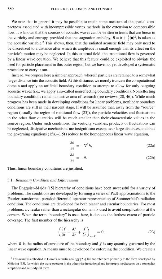
The method was first applied to a pair of identical vortices in a compressible medium. Asthe vortices orbit each other they generate sound at a frequency of twice their rotation rate.The problem has been explored by several researchers (e.g., Muller and Obermeier [38],Yates [48]) and recently simulated by Mitchell, Lele, and Moin [31] using a compact finite-difference method on a stretched grid. The initial configuration of the vortices is depictedin Fig. 4. All quantities are scaled by the initial half spacing between the vortices R andthe ambient speed of sound a∞. For comparison with Mitchell et al. [31], each vortex isGaussian-distributed according to

ω = 1.250

πr20

e−1.25r2/r20 ,

where the circulation and radius of each vortex are 0 = −2π(0.7)−1 M0r0 and r0 = 0.15,respectively. The circulation Reynolds number Re ≡ |0|/ν is 7500, the vortex Mach num-ber M0 ≡ U0/a∞ (where U0 is the maximum azimuthal velocity of a single Gaussian vortex)


y

x2R

2r0

U0

Γ0

FIG. 4. Initial configuration of vortex pair.

is 0.56, and the Prandtl number is 0.7. With these flow parameters, the initial rotation timeis τ = 105 and the wavelength of sound is λ = 52.5. Such a large separation in the acousticand flow length scales qualifies the vortices as a compact source, which makes efficientresolution of the problem difficult. Instead of attempting to capture both the near and farfields simultaneously, the present investigation focused on the near-field dynamics only.The method is capable of computing both, but without particles of variable size it cannotcompute both regions practically.

Initially, the flow is taken as homentropic and dilatation-free. The initial enthalpy isdeduced from a solution of the Poisson equation (20), which is solved with the same Green’sfunction approach used to invert the potential equations (1). The particles are distributedon a Cartesian grid inside a circular domain of radius R with Ncore particles laid acrossthe diameter of each vortex; a boundary zone with a depth of four particles surroundsthe domain. The particles are remapped to the same Cartesian grid every nrm time steps.A fourth-order Runge–Kutta scheme is used for time advancement with a time-step sizeof t = 0.009. The blob radius and particle spacing are related by ε = x0.85. All of thekernels used in the interior are eighth-order accurate, except for the one-sided boundarykernel, which is second-order accurate.

Blob function: ζ(x) = 1π

(4 − 6|x|2 + 2|x|4 − 1

6 |x|6)e−|x|2

Laplacian: η(x) = 1π

(40 − 40|x|2 + 10|x|4 − 2

3 |x|6)e−|x|2

First derivative wrt xi : η(x) = xiπ

(−20 + 20|x|2 − 5|x|4 + 13 |x|6)e−|x|2

Bndry first deriv. wrt xi : ηL(x) = xiπ(−20 + 8|x|2)e−|x|2

To verify that the method converges as the particle coverage is refined, we computed theproblem on a domain of radius R = 2.5 and let Ncore = 10, 13, 20, and 40. The resultingdilatation field at a point (x, y) = (0, 1.2), shown in Fig. 5, converges as the particles aremore densely packed. With 13 particles across each vortex core, the results are sufficientlyconverged.

The results of the vorticity and dilatation fields from a computation with Ncore = 13,R = 4 (corresponding to about 83, 500 particles), and nrm = 2 are depicted in the series of


a∞t/R0 25 50 75 100

-0.02

-0.01

0

0.01

0.02

θR/a

∞

FIG. 5. Dilatation at (x, y) = (0, 1.2). Ncore = 10, · · · · · ·; 13, —·—·—; 20, – – –; 40, —.

a∞t/R = 1.5

a∞t/R = 450

a∞t/R = 65

FIG. 6. Vorticity (left) and dilatation (right) in corotating vortex pair.


a∞t/R = 500

a∞t/R = 600

a∞t/R = 550

FIG. 6—Continued

panels of Fig. 6. Note that both fields are scaled by U0 and R for these figures. For thedilatation panels, dark contours denote positive values and light denote negative. The con-tour levels are as follows: for the first two time levels, the vorticity levels are in the range[−23, −1] in increments of ω = 1 and the dilatation levels are in [−0.06, 0.06] in incre-ments of θ = 0.006; the remaining four time levels have vorticity contours in [−2, −0.05]in increments of ω = 0.103 and dilatation contours in [−0.005, 0.005] in increments ofθ = 0.0005. The first row of panels shows the fields soon after the initialization. Anacoustic transient is emitted from each core as the dilatation settles to the correct value;the transient is not strong and exits the domain without significant reflection. A quadrupolestructure is observed in the dilatation in the next row of panels. The same structure wasobserved by Mitchell et al. [31] as well as by Yates [48] in his Bernoulli enthalpy, a quantitythat is closely related to the dilatation. The configurations of both fields persist for severalrotations, though both quantities are diffused by viscosity over this duration, as observed in


FIG. 7. Histories of the (a) total mass and (b) total circulation of the particles.

the third set of panels (in which the contour levels have been adjusted for better resolutionof the diffused magnitudes). After approximately four rotations the continual effects ofviscosity and compressibility force the cores to merge, depicted in the final three rows ofpanels. The resulting dilatation field is a much weaker quadrupole centered at the core of thenew elliptical vortex. Further computation, not shown, reveals the axisymmetrization of thecore and thus the disappearance of the dilatation.

In viscous vortex methods, an important parameter is the grid Reynolds number, whichcan be defined as Reh ≡ |ω|x2/ν. When Reh = O(1), the smallest length scales in aviscous flow will be well resolved. With Ncore = 13, the particle spacing is x = 0.025, andthus initially Reh,max ≈ 83. This value is significantly higher than the recommended valueof 1. However, computing the same flow with Ncore = 40, corresponding to Reh,max ≈ 7, didnot introduce any new structures. The fine structures in the flow do not appear until latertimes, as depicted in Fig. 6, when the maximum vorticity has decreased substantially andReh,max = O(1).

The conservation properties of the DVPM are demonstrated by plotting the total massand circulation in the domain versus time in Fig. 7. The total mass of the particles rises byless than 0.02% and the total circulation decays by less than 1%. The deviations are duewholly to the fact that the interpolation kernel we have chosen does not exactly conservethe zeroth moment of interpolated quantities, as discussed above. The change in circulationis more dramatic than the change in mass: since only the difference in a particle’s den-sity from the ambient value is interpolated, and |ρ|/ρ∞ is small, the mass is less af-fected by the interpolation error. Neither quantity changes enough to significantly affect theresults.

5.1.1. Kirchhoff surface. Provided that the computational domain extends into theacoustic region, the entire far-field solution can be deduced from the limited acousticinformation available from the near-field simulation through the use of a Kirchhoff sur-face. For a field quantity f governed by the linear, homogeneous wave equation in e, theKirchhoff equation expresses its solution in this domain in terms of its boundary and initialvalues.

In two dimensions, provided that the initial values of f and its derivative are zero inthe exterior domain and on its interior boundary ∂e, the solution f (x, t) in e can be


expressed as

f (x, t) = 1

2π

∫∂e

∫ t∗

0

[(∂ f

∂τ+ f (y, τ )

t − τ + |x − y|)

(eR · ny) − ∂ f

∂ny(y, τ )

]× dτ d S(y)√

(t − τ)2 − |x − y|2 . (30)

The time integral is integrated to the retarded time t∗ = t − |x − y|. The vector eR is theunit vector from the surface position y in the direction of the observation point x; ny is theinward normal at y (or outward from the interior region).

The choice of the variable f in part determines how far one must go from the nonlinearsource region to find the acoustic region. If, for example, the enthalpy is chosen, thenthe region in which this variable is entirely acoustic is apparently quite distant from thesource. Outside of the vortical region, the enthalpy obeys Bernoulli’s equation: h = h∞ −12 |u|2 − ∂χ

∂t , where χ is the scalar potential consistent with the velocity induced by thevorticity. An asymptotic matching of the near- and far-field solutions reveals that, while anexpansion of ∂χ

∂t matches the outer solution term by term, the 12 |u|2 term has no counterpart

in the far field yet persists to large distances because it decays as 1/r2. A more appropriateacoustic variable—consistent with the discussion in Section 3—is the stagnation enthalpyB = h + 1

2 |u|2. In the irrotational region, B = B∞ − ∂χ

∂t , so it satisfies the acoustic equationsjust outside of the vortical region; in the far field, B and h are equal.

The integrals of Eq. (30) are discretized in space and time. A circular Kirchhoff sur-face of radius 3.5 surrounds the vortical region; at this radius it is sufficiently removedfrom the edge of the computational domain to avoid corruption from the boundary treat-ment. The stagnation enthalpy of each particle is computed from the results of the DVPMsimulation and the particle data are interpolated onto the surface control points. The timederivative is computed from backward differencing, and the normal derivative is from a PSEcalculation.

The resulting pressure fluctuations—equal to the stagnation enthalpy after nondimension-alizing—observed at one half-wavelength from the origin (on the y-axis) are depicted inFig. 8. Note that because of the symmetry of the problem each rotation of the vortices

FIG. 8. Pressure fluctuations observed at (x, y) = (0, 12λ). Mitchell et al., –·–; DVPM and Kirchhoff surface

at Rs = 3.5, —; DVPM and Mohring analogy, · · · · · ·.


corresponds to two wavelengths of sound. The magnitude and phase of the pressure agreequite well for the first two rotations. The large spike in Mitchell’s data at the outset isdue to the acoustic transient. Such a spike is not exhibited in the present results becausethe initial transient period is ignored in the Kirchhoff calculation. After a little more thanthree rotations the vortices in Mitchell’s simulation merge, reflected by a small rise andthen quick decay of the pressure. Merger in the present simulation, though, is delayed byan extra one-and-a-half rotations. As demonstrated by Melander et al. [30], incompressiblevortices which are initially separated by more than the critical distance for convectivemerger persist in a “metastable” state for a duration dependent upon a viscous time scale.The vortices eventually undergo convective merger, but the time at which this begins maybe quite sensitive to small perturbations. Thus, it is not surprising that merger occurs laterin our simulation.

5.1.2. Mohring analogy. The compactness of the vortical flow region allows the use ofone of several acoustic analogies for computing the far-field sound. The analogy proposedby Mohring [32] and validated for this problem by Mitchell et al. [31] requires only thethird time derivative of the second moments of vorticity to calculate the pressure at pointsoutside of the source region. The expression for the pressure, adapted to two-dimensionalflow [31], is

p − p∞ρ∞a2∞

= 1

8π

∫ ∞

0

[d3 Q1

dt3(t∗) cos(2θ) + d3 Q2

dt3(t∗) sin(2θ)

]dξ, (31)

where t∗ = t − (r/a∞) cosh(ξ) is a modified retarded time that reflects the dependence oftwo-dimensional sound waves on all events prior to t − r/a∞. The expressions for Q1 andQ2 are

Q1 ≡ 2∫ ∫

xyω dx dy, Q2 ≡∫ ∫

(y2 − x2)ω dx dy. (32)

Clearly Q1 and Q2 are available from an incompressible simulation of this flow usingexisting methods; the far-field analysis considered here is only for completeness. The resultsagree favorably with the Kirchhoff results and those of Mitchell et al. [31], as depicted inFig. 8.

5.1.3. Noncompact flow field. The difficult task of capturing both the near-field dy-namics and the far-field acoustics is alleviated when the acoustic wavelength is not largecompared to the extent of the vortical region. As a further demonstration of the capabilitiesof the DVPM, the same problem was simulated with larger vortex cores, r0 = 0.45, whichcorresponds to a wavelength of λ = 17.5. Larger cores permit a larger region to be coveredby particles. Using the same number of particles as in the previous simulation, the compu-tational domain was enlarged to a radius R = 12. The resulting dilatation field at t = 81is depicted in Fig. 9, with the contour levels saturated to elucidate the outer dilatation. Atthe time shown, the vortices are merging. It is interesting to note that Mitchell et al. [31]did not observe merger after five full rotations, or 175 units of time, using vortices of thesame size but with a much larger Reynolds number. The counter-clockwise tilting of thedilatation structure in the outer regions is due to the phase lag of compressibility.


FIG. 9. Dilatation field at a∞t/R = 81 for a noncompact vortex pair. The contours are saturated for clarity ofthe outer dilatation field.

5.2. Baroclinic Generation of Vorticity

The previous example demonstrated the ability of the DVPM to capture the near-fielddilatation, although the effect of compressibility on the overall flow was quite weak. Thefollowing problem exhibits the capabilities of the method when gradients in thermodynamicquantities are integral to the flow. A planar enthalpy wave travels through an entropy in-homogeneity, or spot, creating vorticity through the baroclinic source term. The resultingvorticity field can be predicted analytically if the wave and spot are sufficiently weak inmagnitude. Suppose that the enthalpy has the initial distribution

h(x1, x2, 0) = h R + h

2

[tanh

(x1 − xh

xh

)− 1

],

and the entropy has

s(x1, x2, 0) = s∞ + s exp

[− (x1 − xs)

2 + x22

σ 2s

],

where h > 0 and s < 0. If both of these quantities are small relative to their ambientvalues, and the entropy is smaller than the enthalpy |s|/|h| 1, then the vorticityapproximately satisfies

∂ω

∂t= ∇h × ∇s,

the enthalpy obeys the homogeneous linear wave equation, and the entropy is steady. Theenthalpy wave travels across the spot at a speed much faster than the velocity induced by


the resulting counter-rotating vortex pair, whose distribution is given by

ω(x1, x2, t) = sh

[tanh

(x1 − xh − t

xh

)− tanh

(x1 − xh

xh

)](x2 − xs)e

−(x1−xs )2−x2

2 ,

where the variables have been scaled by a∞ and σs . We used values of h = 0.01, s =−0.0001, xh = 0.5, xh = −3.5, and xs = 0. For the numerical solution we used particleson a square grid of side length 10σs , with 25 particles across the entropy spot and a boundaryzone at the right (outgoing) boundary with a 4-particle depth, corresponding to a total of14,637 particles. A time step size of a∞t/σs = 0.01 was used. The vorticity that resultsfrom the simulation is shown in Figs. 10 and 11. The agreement is very good.

FIG. 10. Vorticity generated by enthalpy wave/entropy spot interaction at (a) aRt/σs = 0.2, (b) 0.4, and(c) 0.6. DVPM, —; exact, – – –.


FIG. 11. Maximum vorticity generated by enthalpy wave/entropy spot interaction as a function of time.DVPM, ; exact, —.

6. CONCLUSION

A vortex particle method for unsteady two-dimensional compressible flow has been de-veloped. This method is the first Lagrangian method for simulation of the full compressibleequations of motion, though its construction has relied on existing techniques where pos-sible. By using particles that are able to change volume and that carry vorticity, dilatation,enthalpy, entropy, and density, the method satisfies the equations of motion. A scheme forenforcing a nonreflecting boundary condition has also been introduced and successfully im-plemented. The fast multipole method has been adapted to compressible particles for moreefficient implementation. The new vortex method has been applied to corotating vortices ina compressible medium and to the baroclinic generation of vorticity, and the results agreewell with those of previous work or analytical prediction.

Though some previous methods included treatments of compressibility effects (e.g.,[18, 41]) that were useful to the present development, those methods relied on simplifyingassumptions that would preclude direct simulation of the acoustic field. Because of thesmall relative magnitude of the acoustic field, our method requires more delicate applica-tion of techniques that have proven robust for incompressible vortex methods, for instancecomputation of derivatives using PSE (which must now suppress dispersion of waves) andinterpolation during remeshing (which must preserve smoothness in the interpolated quan-tities). This subtle balance comes as no suprise as workers in computational aeroacousticshave long been cognizant of the need for high-order methods (e.g., Lele [28]).

We believe this method shows promise, but further developments are necessary to solveproblems of larger scale. A more “efficient” definition of the particles—for instance, a divi-sion of the particles into those which are active and those which are passive in the velocityinduction—is currently being explored, possibly using domain decomposition techniques.Such a division would permit simulations with two different time steps when the time scalesof physical phenomena in the flow are distinct. Along the same lines, an implementationof the method with variably sized particles, which would allow more efficient resolution offlows with disparate length scales, is under development. Such an extension would makesimultaneous solution of the near and acoustic fields practical. The boundary treatment pro-posed here is sufficient for absorbing incident acoustic waves, but as discussed in Section 3,it does not fully exploit the decomposition of the velocity at the heart of the method. A more


natural scheme is currently being developed. Finally, using existing techniques for comput-ing vortex stretching, we believe that the method is readily extendable to three-dimensionalflows.

APPENDIX: 2-D PARTICLE EVOLUTION EQUATIONS

Here we apply the treatments described in Sections 2 and 3.1 to the equations of motionin two space dimensions and then write the particle evolution equations in their entirety. Towrite them in their most “compact” forms, we define certain shorthand symbols. In PSE,the difference of strengths between two particles is commonly used:

fqp = fq − f p. (A.1)

Many different kernels are used in the method. For instance, in the particle velocities, theregularized kernel is written as

Kε,pq = Kε(xp − xq), (A.2)

the regularized velocity gradient kernel is shortened to(Ri j

ε

)pq

= ∂Kε,i

∂x j(xp − xq), (A.3)

and the PSE kernel is expressed as

η(α1,α2)ε,pq = η(α1,α2)

ε (xp − xq), (A.4)

where the superscript indicates the α1th derivative in the x1 direction and the α2th derivativein the x2 direction. Using this notation, the full equations are

dxp

dt=∑

q

qKε,pq × e3 −∑

q

QqKε,pq , (A.5a)

dp

dt= Vp

ε2

∑q,r

Vq Vr(hq(sr + sq)η

(0,1)ε,qr + hp(sr + sp)η

(0,1)ε,pr

)η(1,0)

ε,pq

− Vp

ε2

∑q,r

Vq Vr(hq(sr + sq)η

(1,0)ε,qr + h p(sr + sp)η

(1,0)ε,pr

)η(0,1)

ε,pq

+ 1

Re

1

ε2

∑q,r

Vp

ρq

[4

3(Vq Qr + Vr Qq)η

(0,1)ε,qr + (Vqr + Vrq)η

(1,0)ε,qr

]

+ Vq

ρp

[4

3(Vp Qr + Vr Q p)η

(0,1)ε,pr + (Vpr + Vrp)η

(1,0)ε,pr

]η(1,0)

ε,pq

− 1

Re

1

ε2

∑q,r

Vp

ρq

[4

3(Vq Qr + Vr Qq)η

(1,0)ε,qr − (Vqr + Vrq)η

(0,1)ε,qr

]

+ Vq

ρp

[4

3(Vp Qr + Vr Q p)η

(1,0)ε,pr − (Vpr + Vrp)η

(0,1)ε,pr

]η(0,1)

ε,pq , (A.5b)

dQp

dt= 2Vp

∑q,r

[q(

R21ε

)pq

− Qq(

R11ε

)pq

][−r(

R12ε

)pr

− Qr(

R22ε

)pr

]−∑q,r

[q(

R22ε

)pq

− Qq(

R12ε

)pq

][−r(

R11ε

)pr

− Qr(

R21ε

)pr

]


− 1

ε2

∑q

VpVqhqpηlapε,pq + Vp

ε2

∑q,r

Vq Vr(hq(sr + sq)η

(1,0)ε,qr

+ h p(sr + sp)η(1,0)ε,pr

)η(1,0)

ε,pq + Vp

ε2

∑q,r

Vq Vr(hq(sr + sq)η

(0,1)ε,qr

+ h p(sr + sp)η(0,1)ε,pr

)η(0,1)

ε,pq + 1

Re

1

ε2

∑q,r

Vp

ρq

[4

3(Vq Qr + Vr Qq)η

(1,0)ε,qr

− (Vqr + Vrq)η(0,1)ε,qr

]+ Vq

ρp

[4

3(Vp Qr + Vr Q p)η

(1,0)ε,pr

− (Vpr + Vrp)η(0,1)ε,pr

]η(1,0)

ε,pq + 1

Re

1

ε2

∑q,r

Vp

ρq

[4

3(Vq Qr + Vr Qq)η

(0,1)ε,qr

+ (Vqr + Vrq)η(1,0)ε,qr

]+ Vq

ρp

[4

3(Vp Qr + Vr Q p)η

(0,1)ε,pr

+ (Vpr + Vrp)η(1,0)ε,pr

]η(0,1)

ε,pq , (A.5c)

ds p

dt= 1

Re

p

ρph p+ 1

RePr

1

ρph pε2

∑q

Vqhqpηlapε,pq , (A.5d)

dV p

dt= Q p, (A.5e)

dh p

dt= −(γ − 1)h pθp + γ

Re

p

ρp+ γ

RePr

1

ρpε2

∑q

Vqhqpηlapε,pq . (A.5f)

The viscous dissipation is computed as

p = 2p

V 2p

+ 4

3

Q2p

V 2p

− 2

∑q,r

[q(

R21ε

)pq − Qq

(R11

ε

)pq

][−r(

R12ε

)pr − Qr

(R22

ε

)pr

]−∑q,r

[q(

R22ε

)pq

− Qq(

R12ε

)pq

][−r(

R11ε

)pr

− Qr(

R21ε

)pr

]. (A.6)

In the boundary zone, Eq. (A.5f) is replaced by the particle form of the boundary condi-tion (24)

dh p

dt= − 1

Rpε

∑q,Rq<Rp

Vqh pq(ηR,(1,0)

pq x p,1 + ηL ,(0,1)pq x p,2

)−h p − 1

γ − 1

2Rp, (A.7)

where Rp = |xp| =√

x2p,1 + x2

p,2 and the notation ηL ,(α1,α2) indicates that the kernel is theleft-sided kernel for approximating the (α1, α2) derivative. The linear combination of kernelsis used to approximate the gradient in the local radial direction (see Fig. 1). Equation (A.7)holds for particles in the boundary zone, but the sum is over all particles, provided thatRq < Rp. This criterion is used to establish that the sum is over the inner half plane,as described in Section 3.1 and derived in [14]. Clearly this restriction corresponds to acircle rather than a half plane, and the intersection of this region with the kernel support


corresponds to a lens-shaped region rather than a semicircle, but the error is smaller thanthe leading-order error in the boundary condition itself. Equation (A.7) is supplemented byEqs. (A.5a) (the boundary particles are allowed to move) and (A.5e). p, Q p, and sp areassumed constant in the boundary region.

ACKNOWLEDGMENTS

The first author gratefully acknowledges support under a NSF Graduate Research Fellowship. This researchwas supported in part by the National Science Foundation under Grant 9501349. A preliminary version of someof the work presented here was reported in [13].

REFERENCES

1. M. Abramowitz and I. A. Stegun, editors, Handbook of Mathematical Functions. American MathematicalSeries (Natl. Bur. of Standards, Washington, DC, 1964).

2. C. Anderson and C. Greengard, On vortex methods, SIAM J. Numer. Anal. 22(3), 413 (1985).

3. C. R. Anderson, A vortex method for flows with slight density variations, J. Comput. Phys. 61, 417(1985).

4. J. T. Beale and A. Majda, Vortex methods II: Higher order accuracy in two and three dimensions, Math.Comput. 39(159), 29 (1982).

5. J. T. Beale and A. Majda, High order accurate vortex methods with explicit velocity kernels, J. Comput. Phys.58, 188 (1985).

6. A. J. Chorin, Numerical study of slightly viscous flow, J. Fluid Mech. 57(4), 785 (1973).

7. B.-T. Chu and L. S. G. Kovasznay, Non-linear interactions in a viscous heat-conducting compressible gas,J. Fluid Mech. 3, 494 (1958).

8. G.-H. Cottet, Artificial viscosity models for vortex and particle methods, J. Comput. Phys. 127, 299(1996).

9. G.-H. Cottet and P. Koumoutsakos, Vortex Methods: Theory and Practice (Cambridge Univ. Press, Cambridge,UK, 2000).

10. S. C. Crow, Aerodynamic sound emission as a singular perturbation problem, Stud. Appl. Math. XLIX(1), 21(1970).

11. G. Daeninck, Local Refinement in Lagrangian Vortex Particle Methods, Master’s thesis (Universite Catholiquede Louvain, 2000). Advised by G. S. Winckelmans.

12. P. Degond and S. Mas-Gallic, The weighted particle method for convection–diffusion equations, Part 1: Thecase of an isotropic viscosity, Math. Comput. 53(188), 485 (1989).

13. J. Eldredge, T. Colonius, and A. Leonard, A Vortex Particle Method for Compressible Flows, AIAA Paper2001–2641 (AIAA Press, Washington, DC, 2001).

14. J. D. Eldredge, A. Leonard, and T. Colonius, A general deterministic treatment of derivatives in particlemethods, J. Comput. Phys., in press.

15. B. Engquist and A. Majda, Absorbing boundary conditions for the numerical simulation of waves, Math.Comput. 31(139), 629 (1977).

16. M. A. Epton and B. Dembart, Multipole translation theory for the three-dimensional Laplace and Helmholtzequations, SIAM J. Sci. Stat. Comput. 16, 865 (1995).

17. D. Fishelov, A new vortex scheme for viscous flows, J. Comput. Phys. 86, 211 (1990).

18. A. F. Ghoniem, A. J. Chorin, and A. K. Oppenheim, Numerical modelling of turbulent flow in a combustiontunnel, Philos. Trans. R. Soc. London A 304, 303 (1982).

19. R. A. Gingold and J. J. Monaghan, Smoothed particle hydrodynamics: Theory and application to nonsphericalstars, Mon. Not. R. Astron. Soc. 181, 375 (1977).

20. D. Givoli, Non-reflecting boundary conditions, J. Comput. Phys. 94, 1 (1991).

21. L. Greengard and V. Rokhlin, A fast algorithm for particle simulations, J. Comput. Phys. 73(2), 325 (1987).


22. O. H. Hald, Convergence of vortex methods for Euler’s equations, II, SIAM J. Numer. Anal. 16, 726 (1979).

23. M. S. Howe, Contributions to the theory of aerodynamic sound, with application to excess jet noise and thetheory of the flute, J. Fluid Mech. 71(4), 625 (1975).

24. O. M. Knio, L. Collorec, and D. Juve, Numerical study of sound emission by 2D regular and chaotic vortexconfigurations, J. Comput. Phys. 116, 226 (1995).

25. P. Koumoutsakos, A. Leonard, and F. Pepin, Boundary conditions for viscous vortex methods, J. Comput.Phys. 113, 52 (1994).

26. A. Krishnan and A. F. Ghoniem, Simulation of rollup and mixing in Rayleigh–Taylor flow using the transport-element method, J. Comput. Phys. 99, 1 (1992).

27. L. D. Landau and E. M. Lifshitz, Fluid Mechanics, Course of Theoretical Physics, Vol. 6 (Pergamon, Elmsford,NY, 1959).

28. S. K. Lele, Computational Aeroacoustics: A Review, AIAA Paper 97-0018 (AIAA Press, Washington, DC,1997).

29. A. Leonard, Vortex methods for flow simulation, J. Comput. Phys. 37(3), 289 (1980).

30. M. V. Melander, N. J. Zabusky, and J. C. McWilliams, Symmetric vortex merger in two dimensions: Causesand conditions, J. Fluid Mech. 195, 303 (1988).

31. B. E. Mitchell, S. K. Lele, and P. Moin, Direct computation of the sound from a compressible co-rotatingvortex pair, J. Fluid Mech. 285, 181 (1995).

32. W. Mohring, On vortex sound at low Mach number, J. Fluid Mech. 85, 685 (1978).

33. W. Mohring, Sound Generation From Convected Vortices, unpublished, 1997.

34. J. J. Monaghan, Particle methods for hydrodynamics, Comput. Phys. Rep. 3, 71 (1985).

35. J. J. Monaghan, On the problem of penetration in particle methods, J. Comput. Phys. 82, 1 (1989).

36. J. J. Monaghan, SPH and Riemann solvers, J. Comput. Phys. 136, 298 (1997).

37. J. J. Monaghan and R. A. Gingold, Shock simulation by the particle method SPH, J. Comput. Phys. 52, 374(1983).

38. E.-A. Muller and F. Obermeier, The spinning vortices as a source of sound, in Proceedings of the Conference onFluid Dynamics of Rotor and Fan Supported Aircraft at Subsonic Speeds, AGARD CP-22 (NATO (AGARD)1967), pp. 22.1–22.8.

39. K. P. Pothou, S. G. Voutsinas, S. G. Huberson, and O. M. Knio, Application of 3-d particle method to theprediction of aerodynamic sound, in Vortex Flows and Related Numerical Methods II European Series inApplied and Industrial Mathematics (Soc. de Math. Appl. & Industr., Paris, 1996), Vol. 1.

40. A. Powell, Theory of vortex sound, J. Acoust. Soc. Am. 36(1), 177 (1964).

41. T. R. Quackenbush, A. H. Boschitsch, G. S. Winckelmans, and A. Leonard, Fast Lagrangian Analysis of ThreeDimensional Unsteady Reacting Flow with Heat Release, AIAA Paper 96-0815 (AIAA Press, Washington,DC, 1996).

42. P. A. Raviart, An analysis of particle methods, in Numerical Methods in Fluid Dynamics, edited by F. Brezzi,Lecture Notes in Mathematics (Springer-Verlag, New York, 1983), Vol, 1127, pp. 243–324.

43. T. Sarpkaya, Computational methods with vortices—The 1988 Freeman Scholar Lecture, J. Fluids Eng. 111,5 (1989).

44. I. J. Schoenberg, Cardinal Spline Interpolation (Soc. for Industr. & Appl. Math., Philadelphia, 1973).

45. M. C. Soteriou and A. F. Ghoniem, On the effects of the inlet boundary condition on the mixing and burningin reacting shear flows, Combust. Flame 112, 404 (1998).

46. S. V. Tsynkov, Numerical solution of problems on unbounded domains. A review, Appl. Numer. Math. 27,405 (1998).

47. G. S. Winckelmans and A. Leonard, Contributions to vortex particle methods for the computation of three-dimensional incompressible unsteady flows, J. Comput. Phys. 109(2), 247 (1993).

48. J. E. Yates, Application of the Bernoulli Enthalpy Concept to the Study of Vortex Noise and Jet ImpingementNoise, Technical Report CR-2987 (Natl. Aeronautics & Space Admin., Washington, DC, 1978).

Documents

A Vortex Particle Method for Two-Dimensional Compressible Flow · His method avoids computing the density gradient in the external force term by tracking this quantity directly rather