Embed Size (px)
Citation preview
SOLUTION OF THE GENERAL BOUNDARY.LAYER EQUATIONS FOR
COMPRESSIBLE LAMINAR FLOW, INCLUDING TRANSVERSE CURVATURE
By
DARWIN W. CLUTTEH and A. M. 0. SMITH
L'
-:porkJ . LB 31088 15 February 1963
PREPARED UNDER NAVY, BUREAU OF NAVAL
WEAPONS, CONTRACT NOw 60-05A3c.
DIr
TISIA 13OOUO FrOIVI/ON
SOLUTION OF THE GENERAL BOUNDARY.LAYER EQUATIONS FORCOMPRESSIBLE LAMINAR FLOW, INCLUDING TRANSVERSE CURVATURE
By
DARWIN W. CLUTTER and A. M. 0. SMITH
Report No. LB 31088 15 February 1963
PREPARED UNDER NAVY CONTRACT NOw 60-0553c,
ADMINISTERED UNDER TECHNICAL DIRECTION
OF THE BUREAU OF NAVAL WEAPONS FLUID
MECHANICS AND FLIGHT DYNAMICS BRANCH, RRRE-4.
Douglas Aircraft Co., Inc. a Aircraft Division a Long Beach, California
1.0 STM4ARY
An accurate and rapid method is presented for solution of the general
equations of compressible, steadyp laminar-boundary-layer flow. The method
allows arbitrary conditions on all of the following: pressure gradientj sur-
face temperature and its gradient, heat transfer, mass transfer, and fluid
properties. Also, the method can calculate the second-order effect of trans-
verse curvature. The only restrictions on the method are that the body be
axially symmetric or two-dimensional and that no dissociation of the fluid
occurs.
The equations that are solved are developed from the Navier-Stokes and
energy equations by an order-of-magnitude analysis. They differ from the con-
ventional boundary-layer equations of Prandtl only in that the second-order
terms that include transverse curvature are retained.
The method of solution consists of replacing the partial derivatives
with respect to the flow direction by finite differences, while retaining the
derivatives in a direction normal to the boundary, so that the partial differen-
tial equations become approximated by ordinary differential equations. Reasons
for choosing this method rather than the more conventional finite-difference
methods are discussed.
Arbitrary fluid properties may be used in the method of solution, that is,
they are inputs in the computer program in the form of formulas or tables as
functions of local enthalpy and pressure. Results obtained with the method
using exact fluid properties for air are compared with those using simpler
fluid-property laws. These simpler laws, which often have been used in the
past in boundary-layer investigations, ere shown often to give poor predic-
tions of heat transfer and skin friction at high speeds.
The method has been programmed on the IBM 7090 computer, and solutions
for a wide variety of flows are presented. Comparisons are made with other
exact and approximate methods of solutions. The flows include cases of heat
transfer, mass transfer, and discontiuities in the boundary conditions over
a large range in Mach number (Mach 0.0 to 10.0). Some comparison with ex-
1
perimental measurement is also made. Also a study of the effect of trans-
verse curvature on the flow over cones is presented. The large number of
calculations and comparisons establish that the method is rapid, highly
accurate, and powerful. It appears capable of solving any flow problem for
which the boundary-layer equations themselves remain valid.
2.0 TABLE OF COT.TVS
Page No.
1.0 Simmary 1
2.0 Table of Contents 3
3.0 Figure Index 54.0 Principal Notation 8
5.0 Introduction 12
6.0 Description of Method of Solution 14
6.1 Boundary-Layer Equations 14
6.2 Transformed Boundary-layer Equations 16
6.3 Fluid Properties 20
6.4 Choice of Procedure for Solution of Boundary- 25
Layer Equations
6.5 Method of Solution of Momentum Equation 28
6.6 Method of Solution of Energy Equation 37
6.7 Finite-Difference Representation of x-Derivatives 40
6.8 Method of Integration 44
6.9 Outline of Procedure for Solving Momentum and Energy 53
Equations Simultaneously
6.10 Starting the Solution 54
6.11 Boundary-Layer Parameters 57
7.0 Character of Solution as Learned from Trial Runs 61
7.1 Similar Flow 62
7.2 Effect of the Various Inputs on the Accuracy of the 65
Solution
7.3 Flow on a Flat Plate with Variable Temperature 71
7.4 Effect of Fluid-Property Laws on Recovery Factor 72
7.5 Comparison of Present Method with that of FlUgge- 73
Lotz and Blottner
7.6 Comparison of Heat Transfer Calculated by the Present 74
Method with that Measured on a Circular Cylinder
7.7 Boundary Layer in an Axisymmetric Convergent-Divergent 75
Rocket Nozzle
7.8 Boundary Layer on a Spherically Blunted Cone at Mach 76
Nubers of 3.0 and 9.0
3
Page No.7.9 Transverse Curvature Effect in Axially Symmetric Flow 80
7.10 Effect of Discontinuities in Surface Temperature and 83
in Wall Mass Transfer on Wall Shear and Heat Transfer
7.i Concluding Statement 87Appendix A - Development of the Boundary-Layer Equations for 88
Compressible Laminar Flow, Including the Effect of Transverse
Curvature
Appendix B - Computer Program for Solving the Boundary-Layer Equations 95
References 101
4
3.0 INDEC OF FIGURSE
No. Title Page No.
1. Boundary layer on a body of revolution. Coordinate system. 15
2. Variation of Prandtl number with enthalpy. Cohen's data of
reference 7 and fitted curve.
3. Notation system for velocity and enthalpy profiles in the 52
boundary layer on a body of revolution.
4. Trial solutions for various values of 911. Stagnation- j5wpoint flow, P = 1.0, R = 0.
5. Notation system for finite-difference representation of 42
x-derivatives.
6. Procedure for starting integration at wall. 52
7. Flow diagram for solving boundary-layer equations at 5
station n.
8. Velocity and enthalpy profiles at Mach number = 3.0 for the 103
similar flow described by P = 1/3, R = 0, gw = 2.0.
Velocity overshoot shown.
9. Heat transfer on a flat plate with variable surface 10i4
temperature. Mach number = 3.0, Pr = 0.72.
10. Dependence of recovery factor on fluid-property laws. 105
11. Comparison of heat transfer calculated by the present method 1o6
with that measured in the wind tunnel for a circular cylinder.
12. Variation of surface distance x, body radius ro, Ue/a*, and 107
M with axial distance for the rocket nozzle problem.e 2 2He = 27.246 x l0 ft /sec ; gw = 0.17625; Pr = 0.78.
13. Results o2 calculation for the rocket nozzle. 10
14. Variation of local velocity, body radiuz and surface distance 109
with axial distance for a spherically blunted cone. M. = 5.0
and 9.0.
15. Results of calculations for the spherically blunted cone at 110
Mach number = 3.0 and 50,000-ft altitude.
16. Results of calculations for the spherically blunted cone at 113
Mach number = 9.0 and 50,000-ft altitude.
5
No. Title Page No.
17. Effect of transverse curvature on shear parameter for flow 82
over a circular cylinder with axis aligned with the flow.
He- 5.0; h/h - l.; lPr O1..
18. Effect of transverse curvature on shear parameter for flow 82
over a cone with axis aligned with the flow. He = 5.0;14
w/h = 5.0; Pr = 1.0; C - 10"; Re = 10 /ft.
19. Transverse curvature effect on shear parameter for flow over 116
a cone for Pr = 1.0; 7 = 1.4. Comparison of present method
with first-order effect of Probstein and ELliott. Pr = 1.0;
C = 1.0; a = 10"; Re = 10 4/ft.
20. Effect of discontinuities in g. on the solution of flow over 117
a flat plate at Mach number = 3.0. Pr = 0.72; C = 1.0;
gw = gw for x S 1.0; g = gw for x > 1.0. Positive valueO Go
of g; means that heat is being transferred to surface.
Negative value means that heat is being transferred from surface
to the air.
21. Enthalpy profiles for two of the flows shown in figure 20. 120
22. Effect of discontinuities in mass transfer on the solution of 121
flow over an insulated flat plate (g = 0.0). M = 3.0;
Pr = 0.72; C = 1.0. Arrows indicate direction of air flow out
of surface.
23. Effect of blowing cold air at the front of a hot flat plate. 12)
Erternal conditions and mass-transfer distributions are the
same as shown in figure 22. Also variation of f'' with xw
is the sane.
24. Effect of blowing hot air at the front of a cold flat plate. 124
U~ternal conditions and mass-transfer distributions are the
same as shown in figure 22. Also variation of f" with xw
is the sane.25. Velocity and enthalpy profiles for one of the flows described 125
in figure 24.
No. Title Pae No.
26. Effect of blowing at the nose of an insulated blunt body on 126
the solution downstream. % = 3.0; Pr = 0.72; C = 1.0;P = 1.0 for x A 1.0; P = 0.0 for x > 1.0. Arrows in-
dicate direction of air flow out of surface.
27. Effect of blowing cold air at the nose of a hot blunt body on 128
the solution downstream. Erternal flow and mass-transfer dis-
tributions are the same as for the flow in figure 26.
28. Velocity and enthalpy profiles for one of the flows described 130
in figure 27.
Appendix
Al Coordinate system for axially symetric body. 89
7
4.o PTI3NCipAL NOTATION
a local velocity of sound
a1 , a2 , .
bl, b2 , constants defined where applicable
c1, c 2 ,*
BI, B21 o.. constant coefficients defined where applicable
CI, C2,
c chord length
cf local skin-friction coefficient, eq.(6.114)
cf skin-friction parameter, eq. (6.116)
Cp specific heat at constant pressure
c _
f nondimensional stream function, defined by eq.(6.7)
F body force
g nondimensional total enthalpy ratio = H/He
h local enthalpy
href reference enthalpy used in fluid property relation from
Ref. 7, = 2.119 x 108 ft2/sec2
2H total enthalpy =h + iu
i count of successive tries in procedure for solving momentum
equation (Appendix B)
unit vector, eq.(A-5)
k thermal conductivity
K bound in computer program on values of pt
L count of successive solutions of the energy equation and
fluid properties in the procedure of solution
m the exponent in the free stream velocity variation, U = c I xm
8
M Mach number
n count of the number of steps in the x-direction
N P + R
p pressurep x due
u dxe
Pr Prandtl number
q heat transfer
Q. count of successive solutions of the momentum equation
in the procedure of solution
r radial distance from axis of revolution
ro radius of body of revolution
rf recovery factor, defined by eq.(7.10)
x drRr dx X
Re Reynolds number = e
St Stanton number, defined by eq.(6.120)
T transverse curvature term defined by Eq.(6.32) except in
Sections 7.3 and 7.4 where it is absolute temperature
uu x ~component of veloci.ty, -=
ev y component of velocity
V vector velocity, eq.(A-5)
x distance along body surface measured from stagnation point
X axial or chordwise distance
body force in x-direction
y distance normal to x
Y nondimensional normal distance, eq.(6 .106)
Y body force in y-direction
9
aangle between normal to the surface y and the radius r
Hartree's measure of free-stream velocity distrioution in
similar flow, 0 = m +---
7 ratio of specific heats, Cp/Cv
B thickness of boundary layer
5 displacement thickness
a dimensionless displacement thickness, eq. (6.103)
a specified accuracy in program
itransformed y coordinate, eq.(6.4)
reither a very large 7j, that is, orutside the boundary layer
or I at the edge of the boundary layer, i.e., = e
B momentum thickness
0 dimensionless momentum thickness, eq.(6.Ui0)
dynamic viscosity
V kinematic viscosity
I variable of integration, or in Section 7.9, a transverse
curvature parameter
'function in energy equation defined by eq.(6.5O)
p density
Tshear stress
(transformed stream function = f - YI, see eq.(6.36 )
*in Section 6.1, a stream function defined by eqs.( 6 .5 and 6.7);
in all other Sections, the enthalpy function g - 1, eq.(6.45)
SUBSCRIPTS
ad evaluated at adiabatic wall
o evaluated at outer edge of boundary layer
10
n evaluated at station n
rec evaluated at recovery temperature, Tree - Tad
ref evaluated ar reference enthalpy
stag evaluated at stagnation point
t evaluated at total temperature
w evaluated at wall
00 evaluated at a reference condition, or see
o usually means evaluated at initial condition, x = 0.
One exception is r0
Primes denote differentiation with respect to 71. fl, etc.
11
5.0 INTRODUCTION
The present work was started because there were many problems of laminar
boundary-layer flow for which no satisfactory solutions had been found.
Among them were questions on high-speed heat transfer and the effects of heat
transfer and wall mass transfer on drag. Answers to these questions require
an exact L!eneral method for solving the boundary-layer equations. Available
methods for solving the boundary-layer equations appeared inadequate. Integral
methods can treat general flows, but they give only approximate solutions.
Similar-flow methods are accurate but are restricted to special pressure dis-
tributions. When the work was started, finite-difference methods appeared to
require unreasonably long computing times for accuracy. Therefore, studies
were made to develop a practical method for solving "exactly" the complete
equations of compressible boundary-layer flow in two-dimensions. The sense
of ''exactly'' as used here is that the solution approaches the exact as the
step length in the calculation procedure approaches zero. The objective of
the studies was to find a method capable of obtaining solutions for arbitrary
values of (1) pressure distribution. (2) wall mass-transfer distribution,
(3) gas properties, and (4) wall temperature distribution. The only re-
striction on the flow was that it be two-dimensional or axially sym.etric.
The problem was approached by first finding a method that gave an ac-
curate solution for the general incompressible boundary-layer equation.
An accurate and rapid method was developed and is presented in References 1,
2, and 3. The method is a modification of the Hartree-Womersley technique.
It consists of replacing the partial derivatives with respect to the flow
direction by finite differences, while re Laining the derivatives in a direction
normal to the boundary, so that the partial aifferential equation becomes
approximated by an ordinary differential equation. The method was programed
on an electronic computer, and solutions for a wide variety of flows were
calculated and are presented in References 1 and 2. The large number of cal-
culations and their comparison with other exact and approximate zolutions
establish that the method is rapid, highly accurate, and powerful. It is
capable of solving any flow problem for which the incompressible boundary-
layer equations themselves are valid. The mathematics of the solution, that
12
is, the behavior of the process of solutions the nature of solutions its
difficultiesp etc., are reported in Reference 3. Also, the reasons for
choosing the present method rather than the more conventional finite-difference
methods are discussed.
After the method of solution had proved successful for incompressible
flow it was extended and modified to solve the fully general laminar boundary-
layer equations for compressible flow. The only restrictions are that the
flow be two-dimensional or axially symmetric and that no dissociation occur
The purpose of this report is to describe this method for solving the
compressible flow equations and establish it validity. Section 6.0 develops
the equations, by starting with the Navier-Stokes equations. The second-order
effect of transverse curvature is retained. Steps in the procedure for solving
the equations are described, and the reasons for choosing them over other
possibilities are discussed. Section 7.0 consists of the results of calcula-
tions of a wile variety of flows. They establish the accuracy of the method.
Wherever possible comparisons of the calculations are made with other methods
and with experiment.
13
6.0 DESCRIPTION OF MlHOD OF SOLUIION
6.1 Boundary-Layer Equations
The problem to be considered is axisymmetric, steady,equilibrium flow
about a body of revolution. The equations necessary to describe such a flow
are those of continuity, momentumi, and energy. Also the equation of state
and relations describing the fluid properties such as viscosity and specific
heat are required.
The problem will be restricted to high Reynolds number, so that the Navier-
Stokes and energy equations are simplified to essentially the form of the
boundary-layer equations as originally developed by Prandtl in 1904. The
second-order effect of transverse curvature that was neglected by Prandtl will
be considered here. Van Dyke considered all second-order effects identified
as: transverse curvature, longitudinal curvature, slip, temperature jump,
entropy gradient, stagnation enthalpy gradient and displacement in a recent
article for the special case of a blunt body (Reference 4). As pointed out
by Van Dyke, logically, all second-order effects should be considered con-
currently, but consideration of all these effects is beyond the scope of the
present work. The effect of transverse curvature is included because of its
importance in predicting boundary-layer growth on long slender bodies, such
as certain missiles.
The basic notation and scheme of coordinates are shown in figure l,where
u is a reference velocity and ue(x) is the velocity of the main flow just
outside the boundary layer. The term He represents the total enthalpy out-
side the boundary layer and is constant. Local enthalpy outside the boundary
layer he is given from the relation
12 12H h +1 u 2 = h + 1 UHe = he +2 e T
The coordinates are a curvilinear system in which x is distance along the
surface measured from the stagnation point. The dimension y is measured
normal to the surface. Within the boundary layer the velocity components are
u and v, being, respectively, in the x and y directions. The body radius
is roe
14
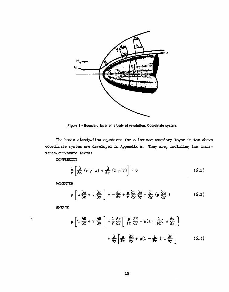
fx
Figure 1.- Boundary layer on a body of revolution. Coordinate system.
The basic steady-flow equations for a laminar boundary layer in the above
coordinate system are developed in Appendix A. They are, including the trans-
verse- curvature terms:
CONTINUITY
_[_ (r Pu) + (r P v)] 0 (6.1)rTy
MOMENTLM
P u + v 6u --- + 6 u+ 6 6 (6.2)
ENERGY
15
Equations (6.2) and (6.3) differ from the forms usually obtained when thePrandtl boundary-layer approximations are madebecause they contain the trans-
verse curvature terms:
Rr in (6.2)
anda n aH + u [( l) u in (6.3)
6.2 Transformed Boundary-Layer Equations
Whereas the above equations could perhaps be solved by the method to bepresented, they will be transformed to a more convenient coordinate system.Flttgge-Lotz and Blottner have solved the above equations essentially as theyare written, though simplified relations for the fluid properties-viscosity
and Prandtl number-were used (Reference 6). The equations as written haveseveral disadvantages; for example, they may be singular at x = 0, and theboundary-layer thickness varies greatly with distance.
These difficulties can be overcome by stretching of the coordinatenormal to the wall y. The transformation that has proven most effective
for accomplishing the stretching is that of Howarth-Dorodnitsyn, where
y
H fp dy
0
=x
It is felt that a second requirement of the transformation of the y-coordinatebe that it should reduce to the incompressible transformation that was studiedextensively by the authors in References 1, 2, and 3. Therefore, consider the
transformation
Ue yS= - fp dy
0 (6.4)X1X
16
Also, it in convenient to describe a stream function * such that
r u--n }(6.5)
pr v--
Furthermore, as was done in incompressible flow, it is convenient to introduce
a dimensionless stream function f such that
f . , u(6.6)
The relation between f and * is
* I .-. x ue f (6.7)
In order to transform the boundary-layer equations above to x, - coordi-
nates, the following relations are used:
a Ue 1 (6.9)
the stream function.
The momentum equation (6.2) becones the following in the transformed
plane:
17
i i (C r fit) + P (- f,2) + FP +1 + R ffi
x- " - = 0 (6.10)
where:
primes denote differentiation with respect to Tj
P L
c -a--- (6.11)Pe 'Le
C -. P (6.12)CO Pe 4~e
du*
-x de = Pressure gradient parameter (6.13)u dx
e
x drR-- - = Radius parameter (6.14)r d~x
For equation (6.10) the boundary conditions are:
= 0 : f'(0) = f = 0 W (6.15)
f (0) =fw
If the wall is impermeable, fw= 0; but with flow through the surface
(p r v) w = -
Then x
(*r)w =- p( ) vw (t) rw(j) di0
In the incompressible reports (References 1, 2, and 3) M was used for thepressure gradient parameter but it is changed here to prevent any confusionwith Mach number.
18
P"a U,
SA r dx (6.16)fw up IwXVP--P, xus rw#x %e ' f w' g
0
Note that vw positive corresponds to blowing; negative to suction. The
outer boundary conditions are
- oo: f' 1-
f '--.0
A few of the more important properties of eq.(6 .10) are noted. If the
edge velocity is of the form ue = clx , (x/ue)(due/dx) is identically P. If
r=clx , R = (x/r)(dr/dx). If P and R are constants it can be shown that
the equation is independent of x and provides the so-called similar solutions.
Equation (6.10) has several advantages over other possible forms. Other
forms are singular at x = 0 and require that an initial profile be specified,
usually some distance from the leading edge; but in (6.10) the term containing
the x-derivatives disappears at the start of the flow, and the solution can
be started with a similar flow. Finally, the equation reduces to the incom-
pressible form which was studied extensively in References 1, 2, and 3. Thus,
not only does form (6.10) have the advantages that are discussed in these
references for incompressible flow, but also the large number of flows studied
there may be used as a check on the present method.
To transform the energy equation (6.3) to the x, I -plane, first define
the enthalpy ratio gH (6.17)
e
and let
-g (6.18)
Then (6.3) becomes
19
2
CO f e J[P1 +R g' + x C(f1 9(.9
2--I g,+ f f
In the solution of (6.19) either the wall temperature or the heat trans-
fer at the wall, corresponding, respectively, to gw and will be specified.
The outer boundary condition is
g(rl -- * 1 as n -0 00 (6.20)
6.3 Fluid Properties
Fluid properties that appear in the momentun and energy equations are
density p, viscosity p, and Prandtl number Pr. These equations were de-
veloped to be valid so long as the fluid is in equilibrium, that is, the fluid
properties are functions only of local conditions - pressure and enthalpy.
Previous investigators have usually used simplified laws for these properties,
such as, a power lw or Sutherland's law for viscosity and a constant value
of the Prandtl number. Whereas it is known that these laws do not accurately
represent the properties over the entire flight regime of interest, the effect
of these inaccuracies on the solution of the boundary-layer equations has neverbeen investigated. The present method of solution has been developed so that
arbitrary fluid properties may be used. That is, they are iuputs in the
program in the form of formulas or tables as functions of local enthalpy and
pressure. There is no restriction on the fluid to be considered, that is,
the flow may be in either airj helium, water, or some other medium. All that
is required is that the fluid be in equilibrium and its properties be specified
in the proper form.
All of the flows to be presented in this report are for air without dis-
sociation. Relations for fluid properties that will be used have been chosen
20
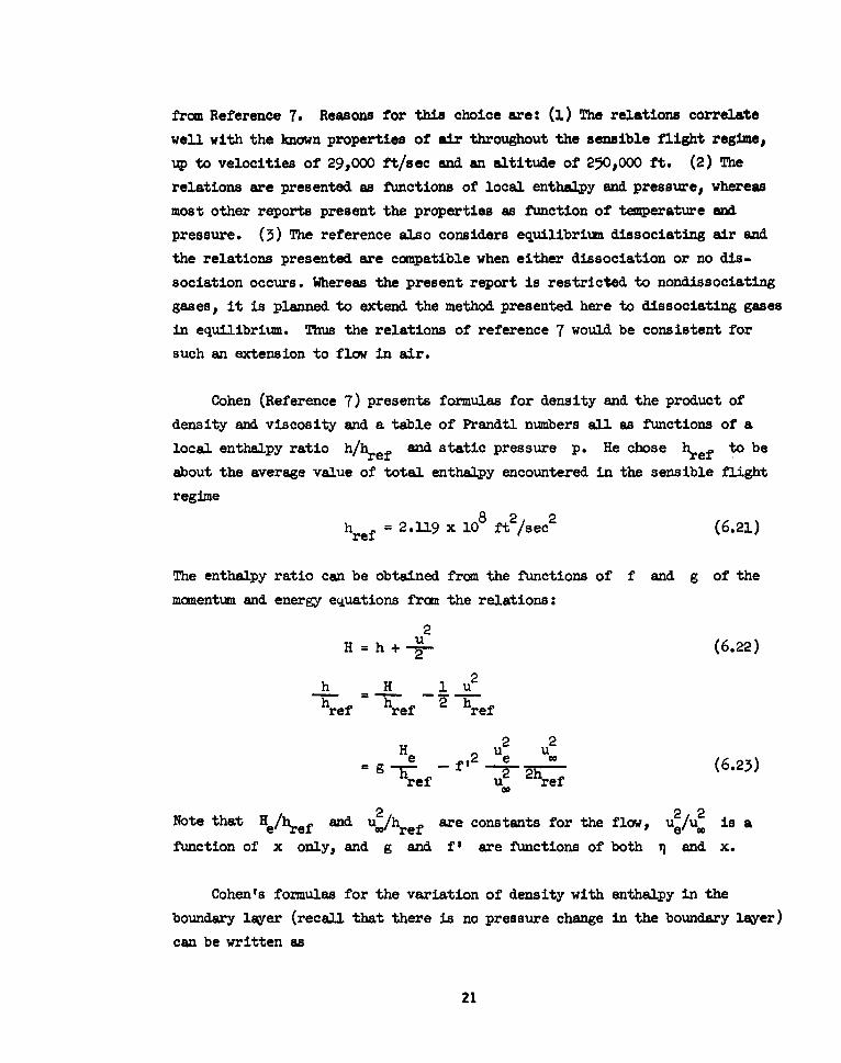
from Reference 7. Reasons for this choice are: (1) The relations correlate
well with the known properties of air throughout the sensible flight regime,
up to velocities of 29,000 ft/sec and an altitude of 250,000 ft. (2) The
relations are presented as functions of local enthalpy and pressure, whereas
most other reports present the properties as function of temperature and
pressure. (3) The reference also considers equilibrium dissociating air and
the relations presented are compatible when either dissociation or no dis-
sociation occurs. Whereas the present report is restricted to nondissociating
gases, it is planned to extend the method presented here to dissociating gases
in equilibrium. Thus the relations of reference 7 would be consistent for
such an extension to flow in air.
Cohen (Reference 7) presents formulas for density and the product of
density and viscosity and a table of Prandtl numbers all as functions of a
local enthalpy ratio h/href and static pressure p. He chose href to be
about the average value of total enthalpy encountered in the sensible flight
regime
h = 2..19 x 108 2 /sec2 (6.21)hrefft/e
The enthalpy ratio can be obtained from the functions of f and g of the
momentum and energy equations from the relations:
2H h + + (6.22)
h H 1 U2
href href 2 href2 2
H u 2 u2_e f12 Ue 09 -T -- - -(6.23)
ref 7 ref
2 2 2Note that H/href and u:/href are constants for the flow, ue/u is a
function of x only, and g and f' are functions of both and x.
Cohen's formulas for the variation of density with enthalpy in the
boundary layer (recall that there is no pressure change in the boundary layer)
can be written as
21
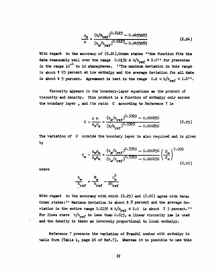
Pe (h/href)0"6123 - 00455283 (6.24)P (he/href)O" 23- 0.0455283
With regard to the accuracy of (6.24.),Cohen states "the function fits the
data reasonably well over the range 0.0152 S h/href ' 2.01, for pressures
in the range 10-4 to 10 atmospheres. "The maximnm deviation in this range
is about t 25 percent at low enthalpy and the average deviation for all data
is about t 5 percent. Agreement is best in the range 0.2 < h/href < 1.6",.
Viscosity appears in the boundary-layer equations as the product of
viscosity and density. This product is a function of enthalpy only acrossthe boundary layer , and its ratio C according to Reference 7 is
p I, (h/h f)3329 - 0.020856C =- = (6.25)
Pete (h/h ref)0 33 9 - 0.020856
The variation of C outside the boundary layer is also required and is given
by
PII .(he/href)0 3329 - 0.020856 p) 0.992
ee (h/hf)' 29 - 0.0256 \-e (6.26)
where2
h H u00 e
h 2heref ref ref
With regard to the accuracy with which (6.25) and (6.26) agree with data,
Cohen states:" Maximum deviation is about t 8 percent and the average de-viation in the entire range 0.0152 " h/href S 2.0 is about t 3 percent."
For flows where h/href is less than 0.015, a linear viscosity law is used
and the density is taken as inversely proportional to local enthalpy.
Reference 7 presents the variation of Prandtl number with enthalpy in
table form (Table 1, page 26 of Ref.7). Whereas it is possible to use this
22
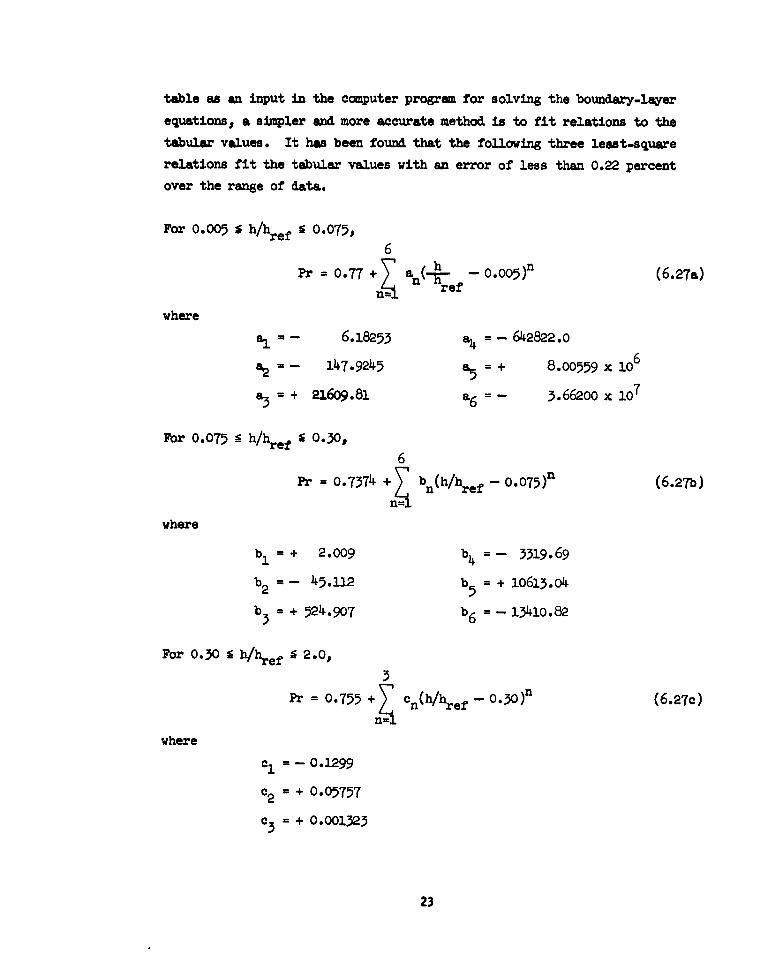
table as an input in the computer program for solving the boundary-layer
equations, a simpler and more accurate method is to fit relations to the
tabular values. It has been found that the following three least-square
relations fit the tabular values with an error of less than 0.22 percent
over the range of data.
For 0.005 S h/href 9 0.075,6
Pr = 0.77 an(- re - 0 . 00 5 )n (6.27a)'1 nref
where
a, = - 6.18253 a4 = - 642822.0
a2=- 147.-9245 a = + 8 .00559 x 106
a3 = + 21609.81 a6 =- 3.66200 x lO7
For 0.075 - h/href ' 0.30,6
Pr = 0.7374 +I bn(h/href -o.075) n (6.27b)
where
bI = + 2.009 b4 =- 3319.69
b2 =- 45.112 b5 = + 10613.04
b 3 = + 524.907 b6 = - 13410.82
For 0.50 h/href S 2.0,
3Pr = 0.755 Cn(h/href _-0.30) n (6.27c)
where
cI = - 0.1299
c2 = + 0.05757
c3 = + 0.00133
23
0.780.78
o DATA PRESENTED BY COHEN REF 70.77 CURVES ARE FITTED BY METHOD
OF LEAST SQUARES
0.75 -
0.75
0.74
Prp0.73-- __
__
__ __
0.72 - - _ _ _ _ _ _
0.71- _ _ _ _ _ _
0.70
0.69
0.68
0.671 1 - -
0 0.2 04 0.6 0.8 1.0 1.2 1.4 1.6 1.8
h AbRE
Figure 2.- Variation of Prandtl number with enthalpy. Cohen's data of Reference 7 and fitted curve.
24
These relations and the tabular values from Reference 7 are plotted in figure 2.
At very low enthalpies, it is seen that the Prandtl number, both Cohen's dataand the fitted curves, increases rapidly as enthalpy decreases. It is believedthat Prandtl number should have a value of 0.72 at the lower enthalpies.Therefore, if h/href < 0.015# this value is used in the program.
Boundary layer in flows of fluids other tian air or in air with otherfluid-property laws can be handled by replacing the relations of this section
by ones appropriate to the flow being studied.
6.4 Choice of Procedure for Solution of Boundary-Layer Equations
The method of sol,,ion will be similar to that used in the study of theincompressible boune _ayer (References 2 and 3). The x-derivatives in the
momentum and energy equations are replaced by finite differencesso that the
partial differential equations are approximated by ordinary differentialequations. Then the problem of solution is essentially to find the unknown
boundary conditions at the wall that satisfy the known outer boundary con-ditions. This is done by a cut-and-try procedure, which is described in
Sections 6.5 and 6.6. The momentum equation (6.10) and the energy equation(6.19) are interdependent and must be solved simultaneously.
Several procedures for solving the equations simultaneously are possible.
Three are:
I. Starting with assumed boundary conditions at the wall, solve the
two equations simultaneously with the appropriate fluid properties.
A cut-and-try procedure would be used on the wall values until the
outer boundary conditions are satisfied.II. To get started, assume an enthalpy distribution (and thus the fluid
properties) and calculate the momentum equation. Again a cut-and-
try procedure would be required. Values of the stream function f
and the velocity f' from the first solution of the momentum equa-
tion would be used in the solution of the energy equation and the
fluid properties. The new fluid properties would be used again to
solve the momentum equation. This iterative procedure would be con-
tinued until convergence of the solution is obtained. A diagram of
25
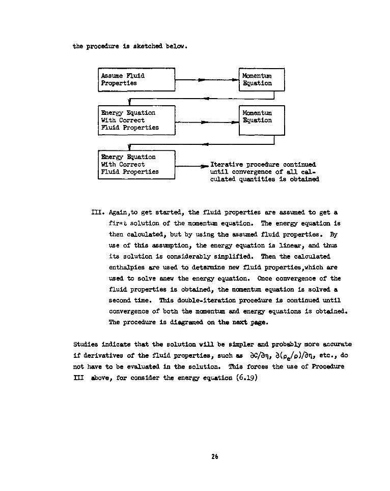
the procedure is sketched below.
IAssume Fluid il Momentum
operties onuation
Energy Equation |MomnentumWith Correct Eq Fuation
Fluid Properties
Energy Equation
With Correct p.Iterative procedure continuedFluid Properties until convergence of all cal-
culated quantities is obtained
III. Again,to get started, the fluid properties are assumed to get a
firs solution of the monentum equation. The energy equation is
then calculated, but by using the assumed fluid properties. By
use of this assumption, the energy equation is linear, and thus
its solution is considerably simplified. Then the calculated
enthalpies are used to determine new fluid properties ,which are
used to solve anew the energy equation. Once convergence of the
fluid properties is obtained, the momentum equation is solved a
second time. This double-iteration procedure is continued until
convergence of both the momentum and energy equations is obtained.
The procedure is diagramed on the next page.
Studies indicate that the solution will be simpler and probably more accurate
if derivatives of the fluid properties, such as aC/a, a(pe/p)/, etc., do
not have to be evaluated in the solution. This forces the use of Procedure
III above, for consider the energy equation (6.19)
26
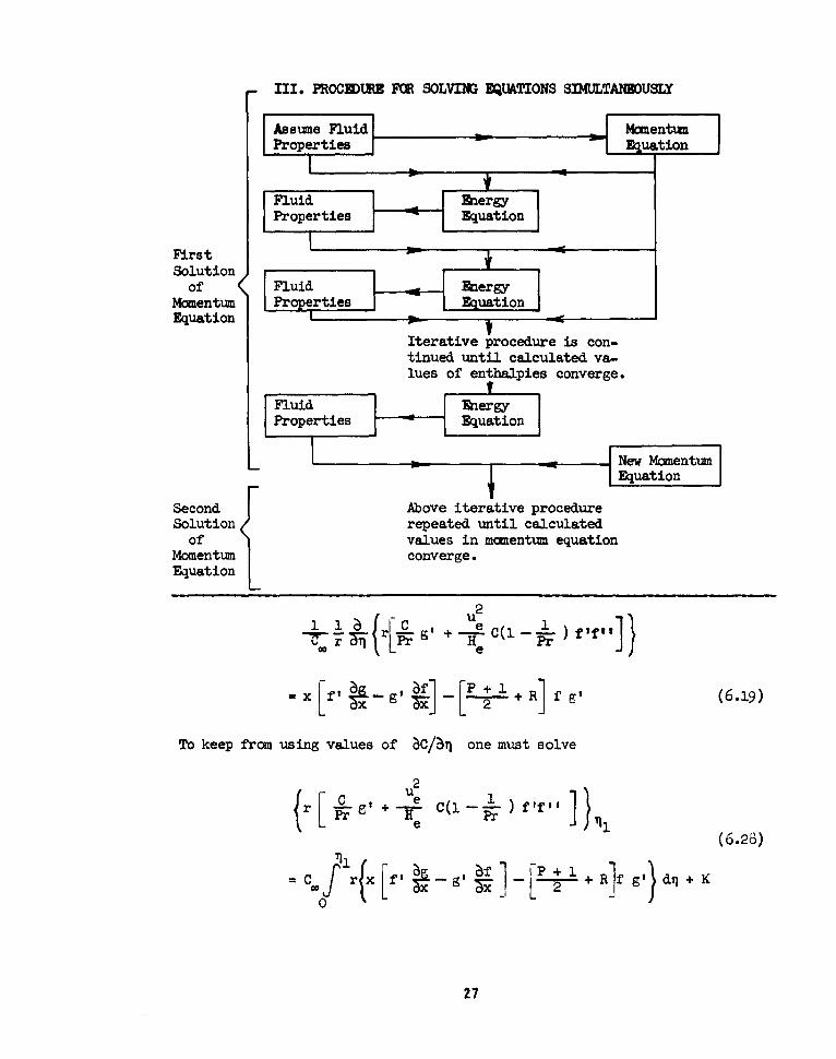
III.* PROCNEUE FOR SOLVIG EUATIONS SIMULTANEDUSLY
Solprttioio
ofFluid EnergyMoenum Properties Euation
EquationtIterative procedure is con-tinued until calculated va-lues of enthalpies converge.
Solution eEaterntlcaclaefPrprte vuE ai oetmuton
Momentumw convrgeEquationoL
Tokefrosn values /in onm sleuto
2
Thus the left-hand side of (6.28) can be determined, but the values of C and
Pr depend on g. which must be determined by integrating g'. An iterative
procedure could be used to determine the value of C, Pr and g', but this can
be avoided by using Procedure III.
Detailed steps in the procedure of solution are given in Section 6.9
and Appendix B.
6.5 Method of Solution of Momentum Equation
Before attempting its solution, equation (6.10) will be rewritten for
simplification. Firstconsider the first term in (6.10)
1 1 (C r f"
The radius r is a function of both x and n, being defined by
r = ro + y cos a = r° + cos a [ f :. d] (6.29)
where r is the local radius of the axisymetric body
a is the angle between the normal to the surface and the radius r
(see Fig. Al).
It would be difficult to handle the integral in (6.29) within the differential
in equation (6.10). Therefore rewrite the first term of (6.10) as
1 l 6 (Cr f") =f1 6 (Cf,) + C. fIl 'cr (6.30)_r F 71-C U
The second term on the right-hand side is the transverse-curvature term and is
negligible when the boundary-layer thickness is small compared to the body radi-
us. Thus there is a second advantage to writing the first term of (6.10) in two
partsin that the transverse-curvature term stands by itself. For further
simplification introduce T, a transverse curvature parameter, defined such
thatI r T2Pe
28
Substitution of the value of r given in (6.29) gives
1r T Pe cos _ _ 1P + y cosa ue P
Cos a PW (6.31)r0 __Iu • iP WU ' P PD
o e (+ p00 Cs-;-VT N- Td)coso =000
Now T may be written as
cos a p
T = Co a PO(6.32)
x u '" ( P00 9W00 0
For simplicity, introduce T which is a function of x onlyU
TV = T(n=0) ~ cos .(632)ro0Jue P.U:X' Pe
Then (6.32) can be written as
TwT w (6.32b)
0
Effects of transverse curvature for particular flows are presented in Section 7.9.
The radius parameter R may be written as
x dr x [dro dos 00 a6,RaFE= ro+Y Cos a+I dx (633)
Now if the boundary layer is small with respect to the body radius, as is
usually assumed in boundry-layer flow, R is simply
29
drR X 0 (633a)
But if it is not, the y terms in (6.33) may affect the solution of the
momentum equation. The last term in (6.33) is
dro dcosa - dr 0 in da-- +Y = dx ysn
--ro [1- d
since sin a = dro/dx. But da/dx is the reciprocal of the local longitudinal
radius of curvature, and this radius must be large with respect to y if
the boundary-layer approximation used in developing the momentum and energy
equations is to hold. That is, if the local radius of curvature is small
with respect to y, the second-order effect of longitudinal curvature becomes
of importance, and the approximation of no pressure change across the boundary
layer is no longer true. Therefore y(da/dx) < < 1 and (6.33) may be written
as
x dro x droR xd~r r0 IF - WE d
rdx l+ YCos cos
0 e 0
x dror. ? U (6.33b)
1 + Pe dniTrf -d
Also for simplicity the symbol N is introduced, defined as
N P + +R (6.34)2
The momentum equation can now be written
30
6 (C f ) =-T -C f"-CP( -f1 2 )-C Nff"+C x ft fU
(6.35)
It will be solved in the same manner as the incompressible equation was in
References 2 and 3. Values of the fluid properties C and Pe/p, which of
course were not needed in the incompressible problem, are assumed here to be
given by the most recent solution of the energy equation. For the very first
solution they are assumed.
In the authors' studies of the incompressible boundary layer it was found
that round-off errors in the computer program could be reduced by substitution
of ' = f' - 1 into the momentum equation (Reference 3). The sane substitu-
tion will be made here. The reason that round-off errors are reduced by the
substitution is that in equation (6.35) all terms approach zero as 71 ap-
proaches oo; both pe/p and f2 approach unity and the round-off error
is primarily introduced when taking their difference. The substitution is9 =f-i 1
'' = f ' (6.36)
P,,,t = f1,,
Introduction into (6.35) gives
6 C, 911) T eCctI+ C C,2 +1 p L
P,, -- , + 2P+ l---
-C N(T + j)99" + C,0x [(q) I+ 1) cpl ] (6.37)
The boundary conditions are now:
=0:
' - 1 (6.38a)
T"= unknown, to be solved for
31
- -F - (PV -- -~J-r
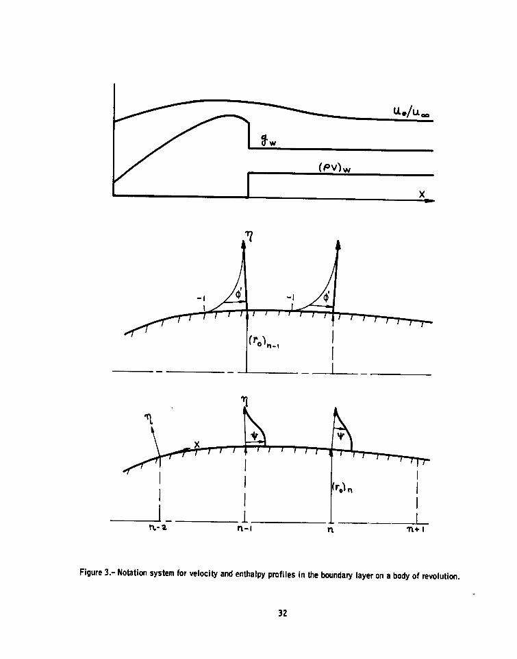
Figure 3.- Notation system for velocity and enthalpy profiles in the boundary layer on a body of revolution.
32
p' --. 0
(6.38b)
The region of solution will be divided into x-wise stations as shown in
figure 3. At each station the x-derivatives will be replaced by finite
differences. The finite-difference representation is described in Section
6.7. This replacement of the partial derivative with respect to x by finite
differences results in an ordinary differential equation at each x-station for
the momentum equation. Each equation must be solved step by step as the cal-
culation proceeds in the x-direction. The equation is third order and non-
linear. Solution of the equation is made difficult by both the nonlinearity
and the fact that one boundary is at n = oo. Ample work in the past has
proved the existence of a solution; therefore it is sufficient to search for
the correct solution. A positive method for doing this is to solve (6.37) as
an initial value problem using arbitrary values of 9" as a third boundary
condition. It is then necessary to search through the possible values of Tw'
to find the one that satisfies the outer boundary condition - that g' ap-
proaches zero asymptotically as I approaches infinity. The procedure for
performing the search is described below but first consider the solution of
tne equation as an initial value problem. First determine
T1
C go" =fr (C (P") dj + Cw cpw (6.39)
0
where (C g") is given by the right hand side of (6.37). C is known or
assumed but cP' is not. It will be found by the searching procedure described
in the following paragraph. The method of integration to be used in (6.39) is
described in Section 6.8. Other quantities needed in the solution of (6.39)
are given by
Cc- =(C (6.4o)C
9' 1 ' d-q-1 (6.41)
0
33
di~ + (6.4.2)
0
Briefly, the procedure for searching for the correct value of q'( is to
first try values of P. until the solutions for p' are bounded in a specifiedregion. Then an interpolation method is used to obtain the value of q'" that
satisfies the outer boundary condition. The steps in the procedure are:
1. Try qp" - (cp")i t, where the latter is an input to the programw w inputor, more conveniently, is the value at the previous station. Compute
outward to determine if the trial solution exceeds P' = 0 or not.
Because of the transformation used, the value of (p' will generallyW
remain between 0 and 4. A value of q1 = 0 corresponds toV
separation.
2. If qp' exceeds 0, the trial value of 1" is high and a secondV
solution is computed with a reduced qp.1. This procedure is continuedw
until both a high and a low value of q" are known.V
3. Once both a high and a low value of q' are known, the bounds on the
correct value of @P' can be further narrowed by splitting the
difference between the upper and lower bounds, and computing again.
4. This splitting the difference can be continued until p" for a highw
solution and c'' for a low solution agree to a specified number of
decimal places. This procedure is positive but costly in computing
time. Studies have shown that the searching procedure can be speeded
up considerably with no loss in accuracy by the following: the split-
ting-the-difference procedure is used until three solutions are ob-
tained such that q' at TLax = % is between the bounds of
-K 9'(%) 9 K. (Both % and K are inputs in the computer
program.) At least one of the three solutions must be high and one
low. A three-point-interpolation procedure is then used to determine
the solution that satisfies the outer boundary condition (P'(%) = 0.
This is the same procedure that was used in the solution of the in-
compressible-boundary-layer equations and reported on in Reference 3.
The interpolation procedure is as follows. Consider the typical set of
trial runs shown in figure 4. The runs are for incompressible stagnation-point
34
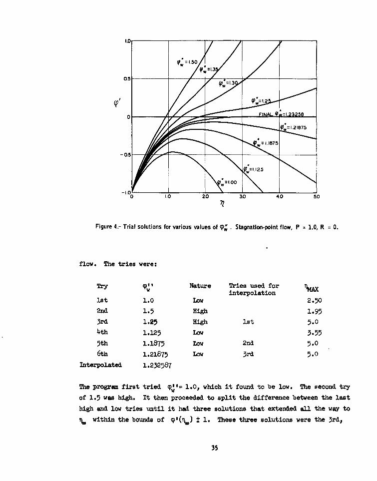
1.50O/
0.5-
-=1.00
0 1.0 2.0 30 4.0 5.0
Figure 4.- Trial solutions for various values of (P; . Stagnation-point flow, P = 1.0, R = 0.
flow. The tries were:
Try Nature Tries used for q1interpolation
1st 1.0 Low 2.50
2nd 1.5 High 1.95
3rd 1.25 High 1st 5.0
4th 1.125 Low 3.555th 1.1875 LOW 2nd 5.0
6th 1.21875 Low 3rd 5.0
Interpolated 1.232587
The program first tried Ip"= 1.0, which it found to be low. The second try
of 1.5 was high. It then proceeded to split the difference between the last
high and low tries until it had three solutions that extended all the way towithin the bounds of (P'(%) ± 1. These three solutions were the 3rd,
35
5thp and 6th trie. Denote than as
lot solution (P (Pl CP{' (C CPt$),I
2nd solution, (2 CP2 (P2 1 C(
3rd solution (P3 P q' (C (P")3
Legrangian three-point interpolation is used to determine the solution which
meets the outer boundary condition 0'( ) = 0. The interpolated solution is
given by
(p (n) = A l(T) + A2 q)2 (n) + A3 C3(n) (6.45)cP'(T) = A. 91.(q) + A2 q)P(n) + A3 cp (P i)
and a similar relation for cpt,(q) and (C qp")t where the coefficients are
given by
T (I-) ( ¢r,)
A C ) cp3'.(r6) (6.44)
A3 = L(.) - c~j(itQ]Lq(P31r) - '(r60 )]
The solution can be made as accurate as desired by restricting the values
of the bounds K. Effect of K on the accuracy of solution is discussed in
Section 7.2. Typically K would have a value of 1 for five-place accuracy.
Computing time required to obtain this accuracy with the interpolation method
is about one fourth the time required if just splitting the difference between
the high and low tries were used. A study showed the thre.-point form of
interpolation to be considerably more accurate than the two-point form. but
no great gains in accuracy were obtained by using more than three points.
36
6.6 Method of Solution of RAergy liuation
Before solving the energy equation (6.19) it is convenient to substitute
the functions T and q introduced in the preceding Section and to also
introduce the function * defined as
*- g-l1 (6.45)
for the same reasons that ( was introduced in the momentum equation. Substi-
tution of the functions in (6.19) gives2
u2 1 p
= -T( ) * + e c(i - - )(P + 1) P,,
- CN(p + n),, + C x [(, + 1) - ' (6.46)
The wall boundary condition are:
at 11 = 0:
(6.47)
A more general boundary condition could be defined by
a= gw + k e
but usually either gw or S , corresponding respectively to wall tempera-
ture and wall heat transfer, would be known.
The third boundary condition is, as i- oo;
(6.48)
*'--. 0
37
The method of solution of (6.46) is similar to that of the momentum
equation. The region of solution is divided into x-wise stations as indicated
in figure 3. Again the x-derivatives are replaced by finite differences ,which
are defined in the next section of this report. When solving (6.46) values
of qp and its derivatives that were determined from the previous solution
of the momentmn equation and fluid properties that were determined from the
previous solution of the energy equation are used. Once a solution has been
obtained the fluid properties are re-evaluated and the energy equation is
solved again. This iterative procedure is continued until convergence of
the solution is obtained. Details of the iterative procedures for solving
both the momentum and energy equations are given in Section 6.9. With these
procedures * and *' are the only unknowns in the solution of (6.46) and
the equation is linear.
The solution of (6.46) is as follows. Rewrite it as
/ a)I+C - * 1= T -a ir - C Ni(cp + + C x (91 + ) .4)
where for siplicity
2- + e C(. - 1 - )(9, + 1) ,, (6.50)
Pr H Pre
Equation (6.49) is integrated to determine 7w
'w =fw, dj + ,(6.i)
0
The method of integration is the samie as for the momentmiz equation and
is described in Section 6.6. From (6.50)
2er C - 1 )(P' + 1) U"1 (6.52)= C L HeP
which may be integrated to determine
1, =J*' & + Vw (6.55)
38
Since equation (6.49) is treated as linear, its solutions may be linearly
combined. It will be solved twiceand the two solutions combined to meet theouter boundary condition. The exact procedure will depend on whether g or
is known.
Case 1: gw is known. Both solutions begin with the same value of *w)
the one imposed by the boundary condition
*(o) = *=w -1
First equation (6.49) is solved by using a trial value of =:
The solution is denoted as
*l(T )
If l(q) is greater than zero,a lower value of * is tried; if itis less, a higher value of *I. The second try is denoted asw
*2(n)The two solutions can be added to produce the most general solution,which can be made to meet the boundary conditions. The general solution
is
*(I) = A *(T() + B *2 (TI) (6.54)
The outer boundary conditions are
) A *(nm.) + B 2(n.) 0
(6.55)v,(O) -.A *j(q) + B *2(q.) 0
and also
But
so that
A+B =
39
Squation (6.55) gives
- 2(n,)A = -(6.56)
and the correct solution is for all I's
*(n) = A *l(n) + (1 - A) *2(1) (6.57a)
and also
*' (TO= A * (n) + (1-A) #p'(T) (6.5Th)
Case 2: g is known.
The procedure is similar to Case 1, but now the energj equation is
solved with two trial values of gw instead of g . Again, the two
trial solutions are denoted as *l(j) and *2(T1). Relations (6.56),
(6.57a),and (6.57b) then may be used to give the correct solution.
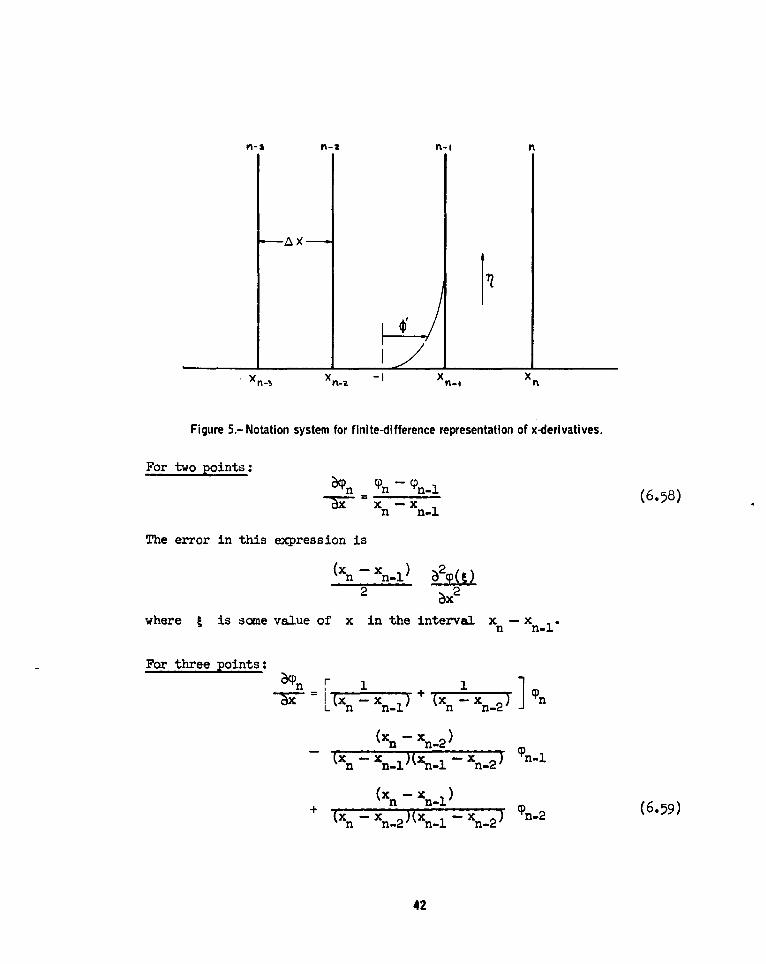
6.7 Finite-Difference Representation of x-Derivatives.
The fundamental idea for the method of solution - that of replacing the
x-derivatives by finite differences to approximate the partial differential
equation by an ordinary differential equation - was advanced by Hartree and
Wamersley (Reference 8). The idea was applied to the incompressible boundary
layer by Hartree (References 9 and 10) and the authors in References 1, 2,
and 3.
Two treatments within the scheme are possible. One is to deal in terms
of the differential equation at a point; in particular, the x-derivatives ata point are replaced by their finite-difference equivalents. Another treat-
ment is to deal in terms of mean values of the variable q or * for aregion of finite extent. Both methods are described in Reference 3. Within
both of the methods there are many possible representations of a derivative
by finite differences, for example, two, three, or more points may be used.
Note that all of the x-derivatives that appear in the momentum and energy
equations are only of first order.
40
In reference 3 the authors made an extensive study of the use of two-
point, three-point, and four-point finite differences in solving the in-
compressible-boundary-layer equations. Both the concept of the point form
and of the mean form were studied. The investigation showed that whereas
the two-point mean representation was more accurate than the two-point point
form, the use of three and four points proved the point forms to be moreaccurate. Solutions obtained by the mean method with the higher number of
points diverged wildly as the step length became small. The same type ofdivergence appeared in Reference 1 where the two-point mean form was used,
but occurred there at much smaller step sizes in x. The investigation alsoshowed that whereas the use of three points in the point form of finite
differences gave a much more accurate solution than the use of two points,further increase of the number of points to four gave no great increase in
accuracy. As a result of the investigation, the three-point point form ofrepresenting the derivatives was chosen in the present method. In addition
to being freer of oscillations as the step size becomes very small, the point
form has the advantages of being simpler conceptually and simpler to programon the computer.
The basic scheme of the finite-difference representation is diagramedin figure 5. The space is divided into a number of regions bounded by linesx n , Xn., Xn. 2 ) Xn. 3 . The spacing A x need not be constant. Because the
momentum equation and energy equation are parabolic in x, the problem mustbe solved by proceeding in the direction of positive x. It is assumed that
the solution has been found at all previous stations up to and includingXn.l, which of course means that cp(TI) and *(T) and their derivatives are
fully known at these stations. The quantity (p'(T) typically has the appear-ance shown in figure 5. The problem is to find the solution CP(r 1) and *(n)
at the new station xn .
Whereas usually three-point finite differences will be used, at the start
of a solution only two points are available and the two-point form must beused. Also, when there are discontinuities in the boundary conditions, it maybe more accurate to use the two-point form. The finite difference repre-
sentations are:
41
M-3 M-2 n-i
-AX
)(n_, Xn-Z -I Xn-I Xn
Figure 5.- Notation system for finite-difference representation of x-derivatives.
For two points:'on Tn - %-l 6-8ax xn - xin
The error in this expression is
(x n - x -l) ec_2
where t is some value of x in the interval x - xn .
For three points:
= (Xn -- iT + (x. n - 2 ) ]jn
(xn - Xn.2 )-x 'n - xn-.)(Xn-l - Xn-2) 'Pn 'l
+ ( n -1 ) (6.59)(xn - x .2)k 1 - Xn-2)
42
A
The error here is
(x, - xn l )(x - x n 2 )
where here g is some value of x in the interval xn - Xn.2.
In solving the boundary-layer equations the quantity aq/ax in both the
momentum equation (6.37) and the energy equation (6.46) is replaced by either
(6.58) or (6.59). The other x-derivatives Zcp'/ax and * /ax are replaced
by similar expressions. When these substitutions are made, it is assumed
that all of the other quantities in the boundary-layer equations are evalu-
ated at xn . The equations are then ordinary differential equations in n
with the variable quantities cp, 91', and * at the n-i and n-2 stations.
Step length Ax is not a primary parameter; instead, x/A x is.
In solving the boundary-layer equations the calculation must start at
x = 0. For the x = 0 station the terms with x-derivives in both the
momentum and energy equations disappear. At the second station the two-point
form of the finite differences is usedbut,at all stations farther downstream
the three-point form may be used. The error in the three-point form is like
3 ax3
as compared to
A x2
for the two-point form. Therefore in order to have the same accuracy in the
solution at all stations the step size at the second station must be suitably
reduced. In practice these errors near the leading edge will probably be
small due to the fact that the flow is nearly similar there, and thus the
x-derivatives are small. But in any case A x can be kept small here, in
order to keep accuracy high.
For further discussion of application of Hartree-Womersley's method for
solution of the boundary-layer equations and the associated errors, see
References 1 and 3.
43
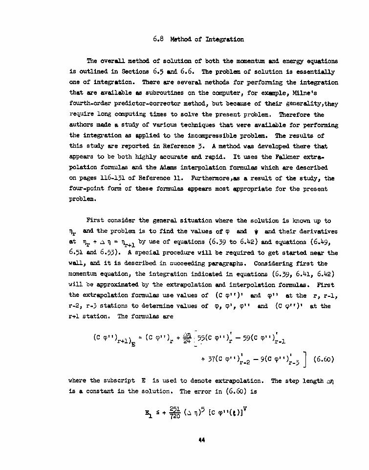
6.8 Method of integration
The overall method of solution of both the monentum and energy equations
is outlined in Sections 6.5 and 6.6. The problem of solution is essentially
one of integration. There are several methods for performing the integration
that are available as subroutines on the computer, for example, Milne's
fourth-order predictor-corrector method, but because of their generalitythey
require long computing times to solve the present problem. Therefore the
authors made a study of various techniques that were available for performing
the integration as applied to the incompressible problem. The results of
this study are reported in Reference 3. A method was developed there that
appears to be both highly accurate and rapid. It uses the Falkner extra-
polation formulas and the Adams interpolation formulas which are described
on pages 116-131 of Reference U2. Furthermoreas a result of the study, the
four-point form of these formulas appears most appropriate for the present
problem.
First consider the general situation where the solution is known up to
r and the problem is to find the values of g and * and their derivatives
at ir + " I = nr+l by use of equations (6.39 to 6.42) and equations (6.49,6.51 and 6.53). A special procedure will be required to get started near the
wall, and it is described in succeeding paragraphs. Considering first the
momentum equation, the integration indicated in equations (6.39, 6.41, 6.42)
will be approximated by the extrapolation and interpolation formulas. First
the extrapolation formulas use values of (C q ")' and g" at the r, r-l,
r-2, r-3 stations to determine values of g, c', c"i and (C 911)' at the
r+l station. The formulas are
(C ,, )r+) (C 9" )r + *2 5 5(C g" )r - 59(C " r-
+ 37(C 9" )- - 9(c g")r._ (6.60)
where the subscript E is used to denote extrapolation. The step length an
is a constant in the solution. The error in (6.6o) is
S + 720 (_ ) (C g (1V
44
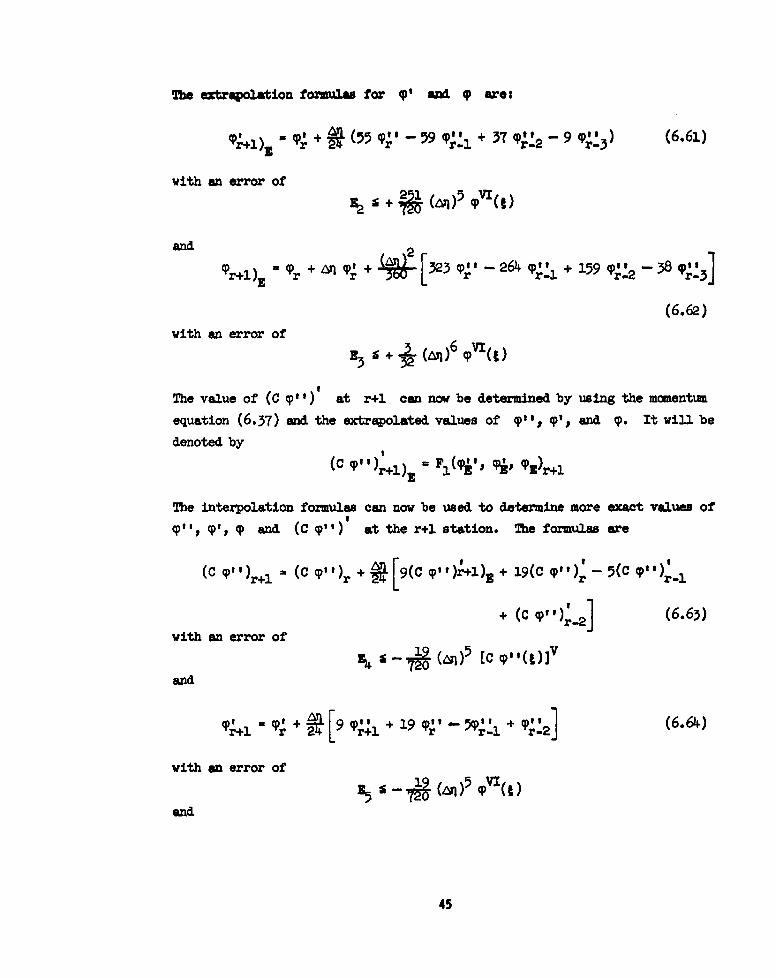
The extrapolation formulas for 4P' and (P are:
I~r+l z Tr + (5 4r 9 r l 3 (r#-# 9 (Pr613
with an error of
and2
(6.62)
with an error of
The value of (C c") at r+l can now be determined by using the momentun
equation (6.37) and the extrapolated values of 4i", ', and q). It will be
denoted by
(C (P,)r+) E = F1 (q,, , q 3)r+i
The interpolation formulas can now be used to determine more exact values of
(P"p qI', q) and (C q9") at the r+l station. The formulas are
(C q) 1 a (C P)r + 4q10994 ) 19c (P ( p )-
with an error of +( P)-](.3
and
+ (P+q)r.q (6.64)
with an error of
and
45
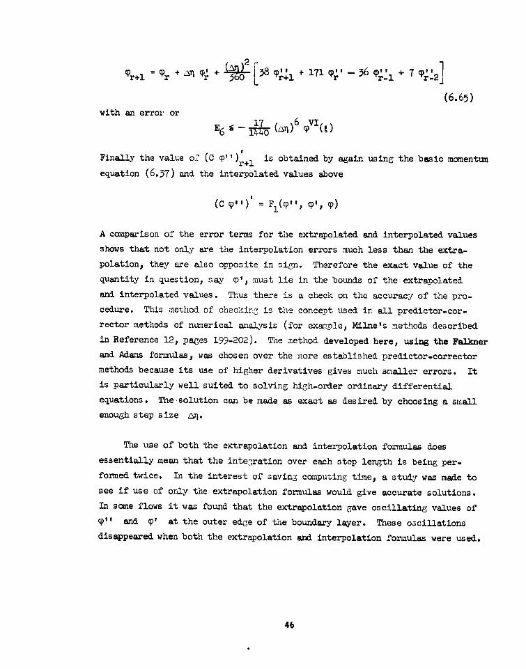
~~r ~ ~ Ia 38 9 +'18~ + 171 CP" 3~6 ep + ~ 7 r21
(6.65)with an error or
Finally the value o.V (C cp'') is obtained by again using the basic momentumr+lequation (6.37) and the interpolated values above
(C cp'') = F1 (cp'', cp', c)
A comparison of the error terms for the extrapolated and interpolated values
shows that not only are the interpolation errors much less than the extra-
polation, they are also opposite in sign. Therefore the exact value of the
quantity in question, say 9', must lie in the bounds of the extrapolated
and interpolated values. Thus there is a check on the accuracy of the pro-
cedure. This method of checking is the concept used in all predictor-cor-
rector methods of numerical analysis (for exa.ole, Milne's methods described
in Reference 12, pages 199-202). The method developed here, using the Falkner
and Adams formulas, was chosen over the more established predictor-corrector
methods because its use of higher derivatives gives much smaller errors. It
is particularly well suited to solving high-order ordinary differential
equations. The-solution can be made as exact as desired by choosing a small
enough step size Arj.
The use of both the extrapolation and interpolation formulas does
essentially mean that the integration over each step length is being per-
formed twice. In the interest of saving computing time, a study was made to
see if use of only the extrapolation formulas would give accurate solutions.
In some flows it was found that the extrapolation gave oscillating values of
ep" and Cp' at the outer edge of the boundary layer. These oscillations
disappeared when both the extrapolation and interpolation formulas were used.
46
The formulas for performing the integrations required in solution of the
energy equation are similar to the above. They are:
for equation (6.51)
l) r + [55 rr - 59 + 9 r-3 (6.66)
for equation (6.53)
a * . [+ 9 + - (6.67)
and froa equation (6.49)
r,+l) , "72(rV' *Z)r+l
The interpolated values are given by
S = 1T+ ~ (9 +) + 19 r' - 5r' + 1 (6.68)
r+l *r + -21 9 *'+l + 19 *'r - 5 *'-1 + *'-2 (6.69)
and finally fron equation (6.49)
'-+l = F2(r', *)r+l
The Starting Procedure.
The extrapolation-interpolation formulas abovc require values of the
variables at four previous T stations. To get started at the wall Taylor's
series will be used. Consider the Taylor's series for C qp"
(C q,,) = (C q),,) + W(C (,,): + C ( ',)( '+
The use of high-order terms in the expansion would require values of the
derivatives of C at the wall, for example, the use of the third term re-
quires the value of
47
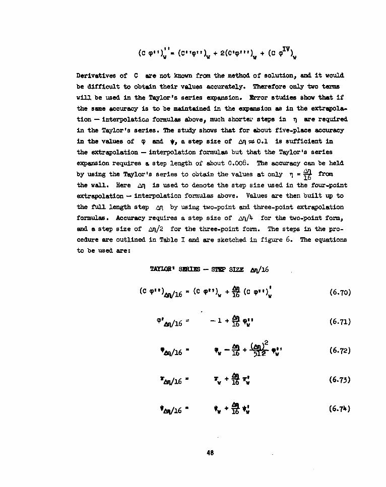
(C V I,)"- (c"(P"f) + 2(C''"), + (C (V)w
Derivatives of C are not known from the method of solution, and it would
be difficult to obtain their values accurately. Therefore only two terms
will be used in the Taylor's series expansion. Error studies show that if
the some accuracy is to be maintained in the expansion as in the extrapola-
tion - interpolation formulas above, much shorter steps in 'i are required
in the Taylor's series. The study shows that for about five-place accuracy
in the values of (p and *,, a step size of Aij d 0.1 is sufficient in
the extrapolation - interpolation formulas but that the Taylor's series
expansion requires a step length of about 0.008. The accuracy can be held
by using the Taylor's series to obtain the values at only I = a from
the wall. Here A'1 is used to denote the step size used in the four-point
extrapolation - interpolation formulas above. Values are then built up to
the full length step A by using two-point and three-point extrapolation
formulas. Accuracy requires a step size of nn/4 for the two-point form,
and a step size of ai/2 for the three-point form. The steps in the pro-
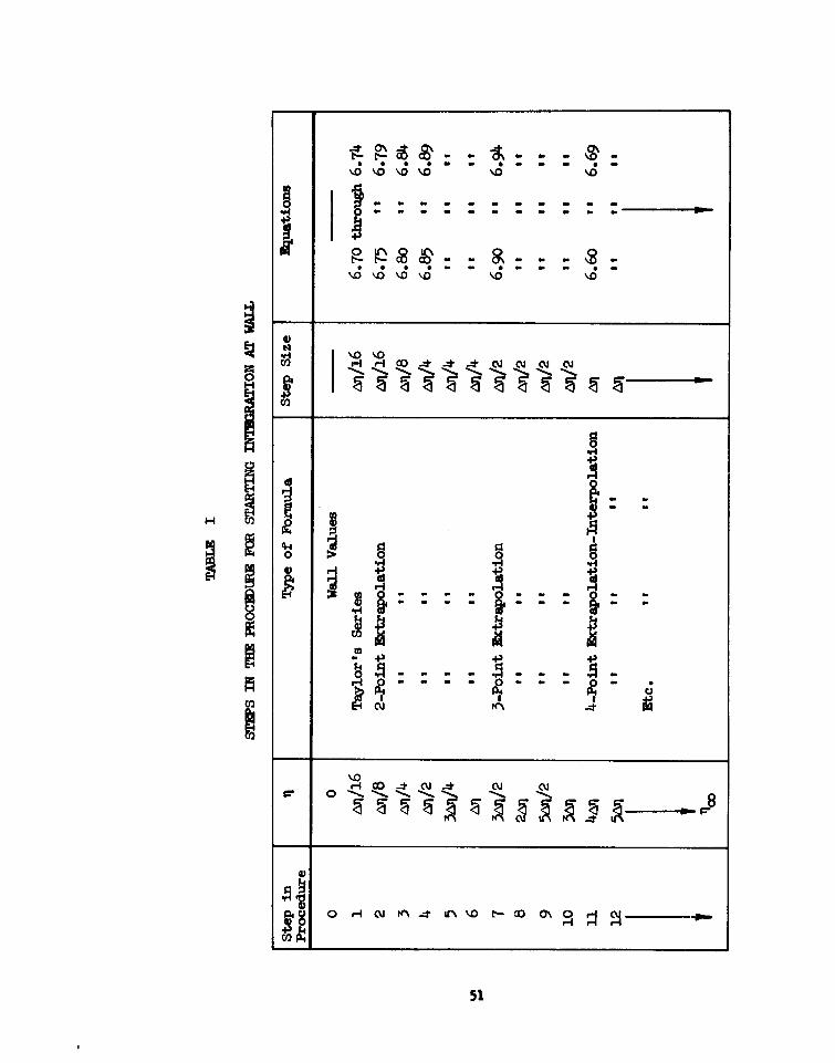
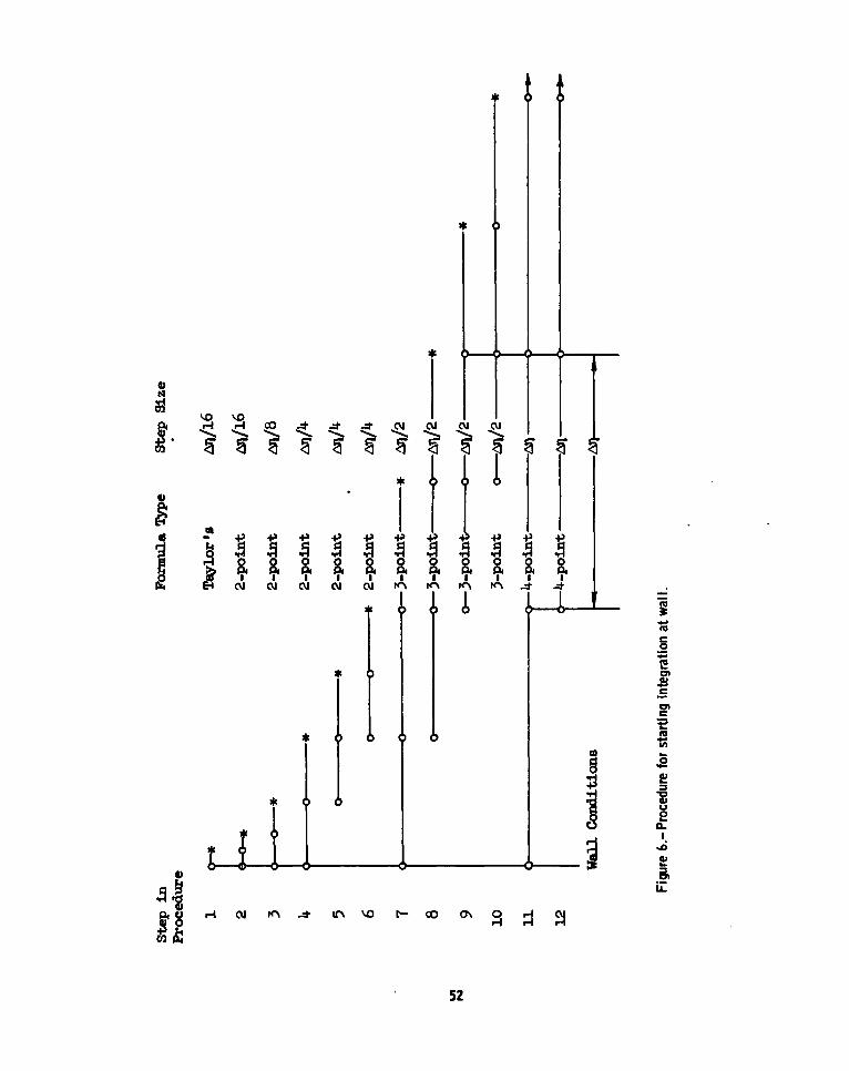
cedure are outlined in Table I and are sketched in figure 6. The equations
to be used are:
TAYLOR, SIES - STEP SIZE An/16
(c '")b,/l6 - (C l")w + -1 (C cps)" (6.70)
PI +(6.71)
9h1/16 = (6.72)l
" ,r + (6.72)
+8(6.74)
48
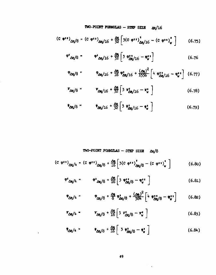
Two-PoIn FmULAS - STEP SIZE an/16
=/1 + an [3( qpl/6 - (C ($1) (6.765
(pt , , /16 + 3 [ q ")6 ['P. o (6T6
-r )(6.78)
*AR/ = *n/16+ -1 [3*1,/6 -(6.79)
TWO-MOINT FOPRLAS - STEP SIZE Aq/8
(C (P),/ = (C 4"),M/8 + -1 [3(C '~) I8 - (C ") 3(6.80)(f ~ 3 q4 4s48+% g8-(. (6.81)
+ (P,;4/8 + ): [/8 - (6. 8]=tq/ -(6.&),M/4; + o '6/8 r , -,, (6.83)
-(6.84)
49
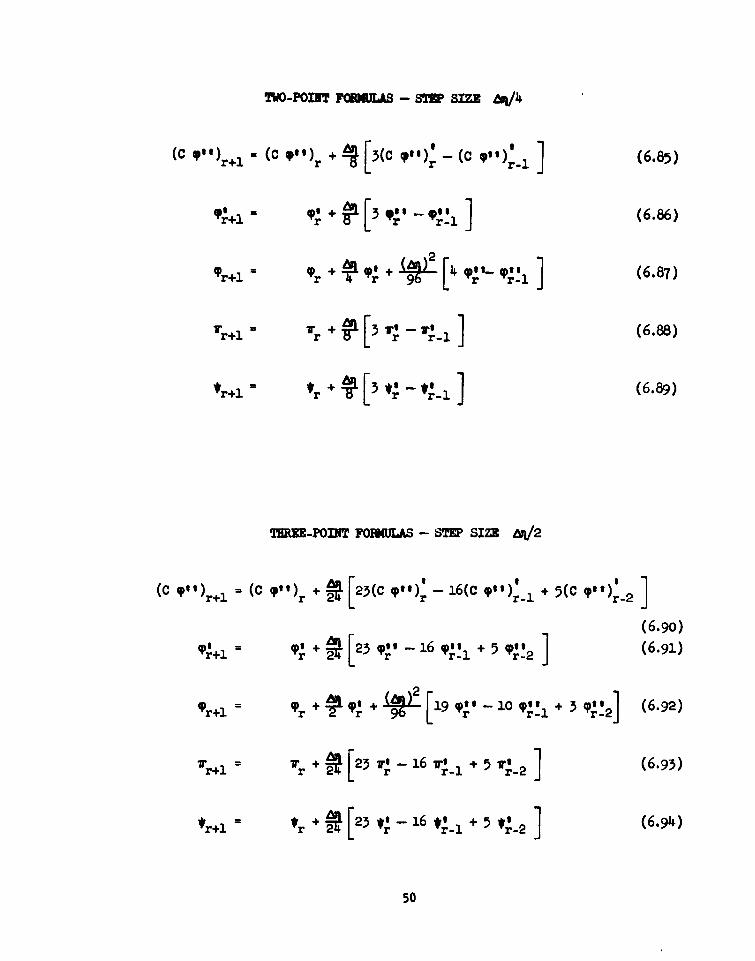
Two-POINT FamuLs - STEP SIZE b/i
(c gp")r+l (c 91)+ [3(C P"); - (C (P"):-] (6.85)
r" + [3 9 I- Pr 1 (6.88)9r+1 lror rl
7+ Ub 3 - r'_ ] (6.88)
TaU-pOIT FODUJLAS - STEP SIZE Aq/2
(c "~~ (c 4?")r + 24 [23(C p") 16(C 4"' ):- + 5(c vt 1)-2]
- (6.90)
9or + 4r + L)qL[19 4pl -10 Pr 1+ 3 Tr 1 (6.92)
+ -21[23 ie- 16 w~~j+ 5 .02] (6-93i)
50
* 17, - - * -
I I
sr 0 4< Sul)
0 ~ ~ 0 m -t n'D I o
51
*ftA6 0
522
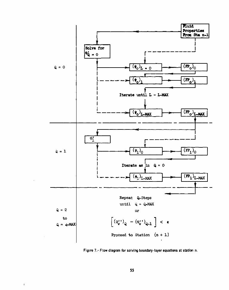
6.9 Outline of Procedure for Solving Mmentum and Nwrgy SquationsSiultaneously
The procedure for solving the momentum and energy equations is briefly des-
cribed in Section 6.4, and the reason for its choice is discussed there. Details
of the procedure are given in this section. Consider the general case when the
program is solving the equation at the n-station. Values of c and * and their
derivatives at all previous stations will be known. First the momentum equation
is solved using the fluid properties from the n-1 station. The values of 's
from this solution are used to solve the energy equations but still using the
fluid properties from the n-i station. Then new fluid properties are determined
and an iterative procedure followed until convergence of solutions of both the
momentum and energy equations is obtained. In the iterative procedure let (4 = i
(an integer) indicate one solution of the momentum equation with the accompanying
solutions for enthalpy and fluid properties. The procedure is:
(a) The momentum equation is solved by using the fluid properties from
the n-i station. It is solved by the cut-and-try and interpolating
procedure described in Section 6.5. The solution is denoted as To.
(b) The energy equation is solved by using the po value and the n-i
fluid properties. The solution is denoted as (*o)L-OS where L is
a count of successive solutions of the energy equation and fluid
properties at a given Q.
(c) The solution (*o)L=O is used to determine new fluid properties.
They are denoted as (FPo)L=O.
(d) The fluid properties (FPo)L=0 and the solution go are used to
obtain a second solution to the energy equation (*o)L-l and new
fluid properties (P% L-l(e) This iterative procedure is continued until L - L-MAX. Proceed
to -= 1.
(a) The momentum equation is solved a second time by using fluid proper-
ties (po)L.MA X and the solution is denoted as 91.
(b) steps (b) through (e) in Q = 0 are repeated to obtain (*I)L.MAX •
53
> 1
(a) The procedure in Q = 1 is repeated, using always the latest values
of (p), (*), and (FP) until either
or(P)w - (CP' < 6w ' w )Q-2.
where a is an accuracy input. If either of these conditions
is satisfied, the program proceeds to the next station.
The procedure is sketched in figure 7) and further details of the
computer program are given in Appendix B.
6.10 Starting the Solution
At x = 0 the x-dependent terms disappear in both the momentum and
energy equations. The equations reduce to:
C c -L T C I'' + C ( '2 + 2 V + 1 -- -- C N(P + )m''
(6.95)
for momentum and
u2*, + eC(l - P +,, 1) ,,
2
Pe C_ #j +-e C(l- )(9' + 1) C" I-C N(9 + n) ' (6.96)
for energy. Hence values of q and * at previous stations are not required.
The x-dependent terms also disappear for similar flows. Such flows occur when
P) R and the wall boundary conditions are constants for all x's. They in-
clude those with constant pressure, such as flows about a flat plate and
wedges. Similar llows are discussed more completely in Chapter 8 of Hayes
and Probstein, Reference 13.
54
I IterateseiniQs
2 or
to F
Proered toSttion (n .q.1)
Fiur 7- lo dagamfo o)lbu-laye eqaiosat taioXn
55.....
The procedure of solution requires that the momentum equation be solved
first, but to do so requires values of the fluid properties. At a downstream
station the properties are approximated for the first solution of the momentum
equation by assuming then to be the sane as those at the previous station. To
get started at the x = 0 station, a linear enthalpy profile that satisfies
the inner and outer boundary conditions for enthalpy is assumed. The fluid
properties obtained fran this enthalpy profile are then used to start the
solution. After the first solution of the momentum equation at any station
is found, the fluid properties obtained from the latest solution of the energy
equation are used for subsequent solutions of the momentum equation. The
iterative procedure is presented in the preceding section of this report.
Values of P and R
The values of P and R are either inputs in the program or are cal-
culated from the velocity distribution ue versus x, and the radius distri-
bution r0 versus x. They are defined by
=(u ~)n
n r r n
x d
1 + T P ~
Both Pn and (ro/x)(dro/dx) are always inputs at x = 0, but may be calculated
at aft stations by use of Lagrangian derivative formulae
d' n = An -l u + A u + An+ u (6.97)nien.i n e n+J eCn+ 1
and n= A, 1 r +An r + An+, r (6.98)
°n-1 On °n+I
where
56
xn - n+iA - n - x(ni Xn -7A l Xn-i - xnAXn-l - i
2Ax -x+l - x-l (6.9)
A x =n (n n +
6.11 Boundary-Layer Parameters
Once the profiles of ( and * and their derivatives have been de-
termined at an x-station, the program determines the conventional boundary-
layer parameters of displacement thickness, momentum thickness, local skin
friction and local heat transfer. First the profiles of (), *, and their
derivatives are transformed to the more conventional profiles of the stream
function f, the velocity ratio f', enthalpy ratio g, etc.
The displacement thickness is calculated from the well known formula
8 =f (l - ) dy (6.100)
In the true definition of a displacement thicknessequation (6.100) is exact
only for two-dimensional flow. For axially symmetric flow the exact dis-
placement thickness is given by the quadratic equation
8"(l+ - cos a) (1 + -Z- cos a)(1 - dy (6.101)2r 0 x)=rl+ 0 csael Q L d0
Because of difficulties in solving (6.101), the simpler expression (6.100) is
used to calculate displacement thickness for all flows. Transforming to the
x, n coordinates, (6.100) is
57
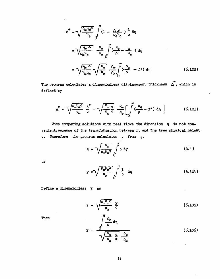
U
e 0 PeUe P
= ./" -' P.o ( P aV p P ee
U - ra-f' (6.lo2)
-VUGOP--- Ue Pe0
0*
The program calculates a dimensionless displacement thickness A which is
defined by
* U 8* U Pi_-ii" u -PL (-e -fl) dji (6.103)
When comparing solutions with real flows the dimension i is not con-
venient, because of the transformation between it and the true physical height
y. Therefore the program calculates y from 7.
: e (6.4)
0
or
= f ' dn (6.lo4)
Define a dimensionless Y as
y = Yc (6.105)
c
Then f-d
0 (6.lo6)
=3F Pe
58
Introduction of Y in (6.103) gives
-- U u a fl (6.1o7)
The momentum thickness is given by
o- f u( u y (6.lo8)0 Pe Ue ue
or in x, n coordinates by
U 0 f_ f l f ) d q (6 .1 0 )ow~u -e Pe 0f
The program calculates a dimensionless momentumn thickness defined as
PW -' v. - (6.1o0
or
uW P- z f,) dn (6.13.)P0
The shear stress at the wall is
w V ww (6.112)
or in x, q coordinates
SV . P f (6.u13)
Introduction of the local skin-friction coefficient defined as
59
cf w 2 (6.114)
gives
cfU=2 (u)3/2Pw ft (6.115)
A conventional shear parameter is
c c_ = 2( ) /fi (6.116)
The heat transfer at the wall is
Now.1 = (3_ -- (u r (6.3.8)
w~ = W[
since uw = 0. Heat transfer in x, coordinates is given by
- e w1 - He (6.119)
The Stanton number., a heat transfer parameter, is defined as
= Ue 9ww 1(6.12o)
UpU H - H) 1P.. e w pwx u p r 8
The ratio of Stanton number to skin friction is given by
St Uo2 u (6.121)
w e w
* The Stanton number is most often written in terms of Hrec -H rather
than He - Hwj but this is not convenient in the present method.
60
7.0 CHARACTER OF SOLUTION AS LIARN FROM TRIAL RUNS
The principal purpose of this section is to establish the accuracy and
character of the method of solution. It will be done by presenting a large
number of flow cases that include large ranges in pressure gradient, heat
transfer, transverse curvature effects, and different fluid-property laws.
Whenever possible, comparisons are made with exact solutions or with experi-
ment. Also, in some cases comparisons are made with approximate methods of
other investigators. Section 7.1 discusses the accuracy for similar flows.
Since these are almost the only flows for which exact solutions are available,
they are used to study the effect of the various inputs in the computer pro-
-gram on the accuracy of the calculations in Section 7.2.. Section 7.3 compares
the present method of solution with that of Chapman and Rubesin for the special
case of a flat plate with variable wall temperature. Effect of the various
fluid-property laws on recovery factor is determined in Section 7.4. Section
7.5 compares the present method with the finite-difference method of Fltfgge-
Lotz and Blottner. The present method is compared with experimental results
for the special case of a circular cylinder in Section 7.6. An example of
internal flow, the boundary layer inside a nozzle, is presented in Section 7.7.Boundary layers on a reentry-type body are presented in 7.8 showing the effect
of altitude, body temperature, and the fluid-property laws on the solutions.
Transverse curvature effects are studied in 7.9. Finally, in Section 7.10,discontinuities in body temperature and mass transfer are studied. This study
is applicable to some types of ablation cooling.
The first - and an obvious - check of the program was simple incompressibleflow. For such flow the equations reduce to the form presented in References
1 and 2, where the authors developed the present method of solution for in-
compressible flow. Many of the cases presented in References 1 and 2 were
recalculated by the present method. Results were identical to the earlier
ones and will not be repeated here. Since the energy equation is negligible
and fluid properties are constants for incompressible flow, these cases affordeda check on only ihat portion of the program that solves the momentum equation.
61
7.1 Similar Flow
Since almost the only flows for which highly accurate solution are known
are the similar flows calculated by Cohen and Reshotko (Reference 14), these
were first used to check the programing of the equations. Similar flow occurs
when the solution is a function of q only, that is, when f and g and their
derivatives are independent of x. In their method Cohen and Reshotko used
Stewartson's transformation to transform the compressible equation to an in-
compressible form. Specifically. the transformations are:
x
Pe ae d. (7.1)PI T aTx
y= ae P
a' fd (7.2)
0
a u (7.3)ae
where here X, Y, and U are the transformed quantities, the subscript T
refers to free-stream stagnation valuesp a is the velocity of sound, and
X is a constant in a linear viscosity-temperature relation. The transformations
are restricted to the case where viscosity varies linearly with temperature and
for Prandtl number 1.0. The same assumptions are used in the present method when
comparing its results with those of Cohen and Reshotko. Similar flow occurs
whenU = c (7.4)e
Cohen and Reshotko present their results for specific values of the pressure
gradient parameter P, which is related to m by
m+ 1
Results of the present method are compared with those of Cohen and Reshotko
in Table II for various values of m and g. In the present method the calcu-
lation can be compared directly with Cohen and Reshotko's results by letting
62
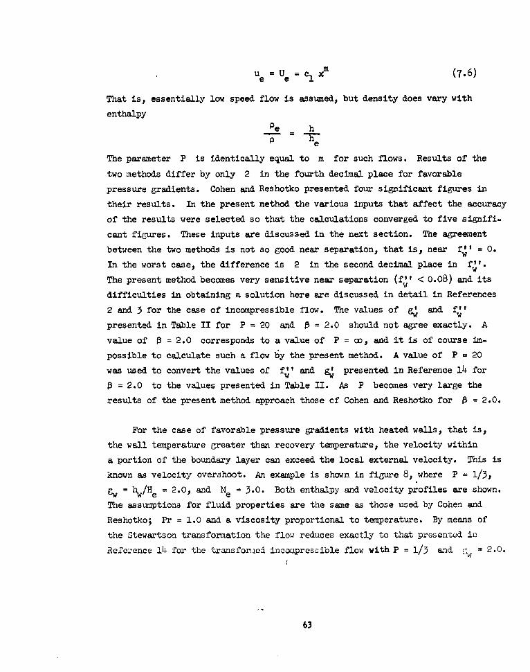
ue =U e =cl xm (7.6)
That is, essentially low speed flow is assumed, but density does vary with
enthalpyPe h
P e
The parameter P is identically equal to m for such flows. Results of the
two methods differ by only 2 in the fourth decimal place for favorable
pressure gradients. Cohen and Reshotko presented four significant figures in
their results. In the present method the various inputs that affect the accuracy
of the results were selected so that the calculations converged to five signifi-
cant figures. These inputs are discussed in the next section. The agreement
between the two methods is not so good near separation, that is, near f' = 0.w
In the worst case, the difference is 2 in the second decimal place in f".W
The present method becomes very sensitive near separation (f" < 0.08) and itswdifficulties in obtaining a solution here are discussed in detail in References
2 and 3 for the case of incompressible flow. The values of f and f'w
presented in Table II for P = 20 and 0 = 2.0 should not agree exactly. A
value of 0 = 2.0 corresponds to a value of P = co, and it is of course im-
possible to calculate such a flow by the present method. A value of P = 20
was used to convert the values of f" and presented in Reference 14 forw= 2.0 to the values presented in Table II. As P becomes very large the
results of the present method approach those of Cohen and Reshotko for 0 = 2.0.
For the case of favorable pressure gradients with heated walls, that is,
the wall temperature greater than recovery temperature, the velocity within
a portion of the boundary layer can exceed the local external velocity. This is
known as velocity overshoot. An example is shown in figure 8, where P = 1/3,
gw = hw/He = 2.0, and Me = 3.0. Both enthalpy and velocity profiles are shown.
The assumptions for fluid properties are the same as those used by Cohen and
Reshotko; Pr = 1.0 and a viscosity proportional to temperature. By means of
the Stewartson transformation the flow reduces exactly to that presented in
Refel-ence 1L for the transfon.aed incompressible flow with P = 1/3 end = 2.0.
63
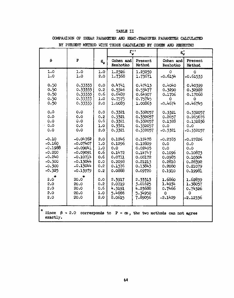
TABLE II
COMPARISON OF SHEAR PARAMETER AND HEAT-TRANSFER PARAMETER CALCULATED
BY PRESET METHOD WITH THOSE CALCULATED BY COHEN AND RESHOTKO
wP 9w Cohen and Present Cohen and Present
Reshotko Method Reshotko Method
1.0 1.0 1.0 1.2326 1.23259 0 01.0 1.0 2.0 1.7368 1.73671 -o.6154 -0.61533
0.50 0.35553 0.0 0.4741 o.47413 O.4040 o.403990.50 0.33333 0.2 O.5346 0.53477 0.3290 0.329220.50 0.33333 0.6 o.6489 o.64907 0.1706 0.170680.50 0.33333 1.0 0.7575 0.75745 0 00.50 0.33333 2.0 1.0085 1.00863 -o.4674 -o.46745
0.0 0.0 0.0 0.3321 0.332057 0.5321 0.3320570.0 0.0 0.2 0.3321 0.332057 0.2657 0.2656760.0 O.0 o.6 0.3321 0.332057 0.1328 0.1328380.0 0.0 1.0 0.3321 0.332057 0.0 0.00.0 0.0 2.0 0.3321 0.332057 -0.3321 -0.332057
-0.10 -0.04762 2.0 0.1246 0.12478 -0.2783 -0.27826-0.160 -0.07407 1.O 0.1296 0.12809 0.0 0.0-0.1988 -0.09041 1.O 0.0 0.02405 0.0 0.0-0.200 -0.09091 o.6 o.1472 0.14747 0.1096 0.10873-0.240 -0.10714 o.6 0.0711 0.08172 O.0985 O.10304-0.300 -0.13044 o.0 O.2098 0.21213 O.2810 o.28392-0.300 -0.13044 0.2 0.1376 0.13843 0.2080 0.21079-0.325 -0.13979 0.2 0.0888 0.09720 0.1910 o.19981
2.0 20.0 0.0 2.3917 2.33313 1.6860 1.628392.0 20.0 0.2 2.0719 3.01625 1.4034 1.380572.0 20.0 o.6 4.3191 4.23688 0.7466 0.743262.0 20.0 1.0 5.4666 5.34950 0 02.0 20.0 2.0 8.o615 7.89056 -2.1429 -2.12336
Since = 2.0 corresponds to P = a, the two methods can not agreeexactly.
64
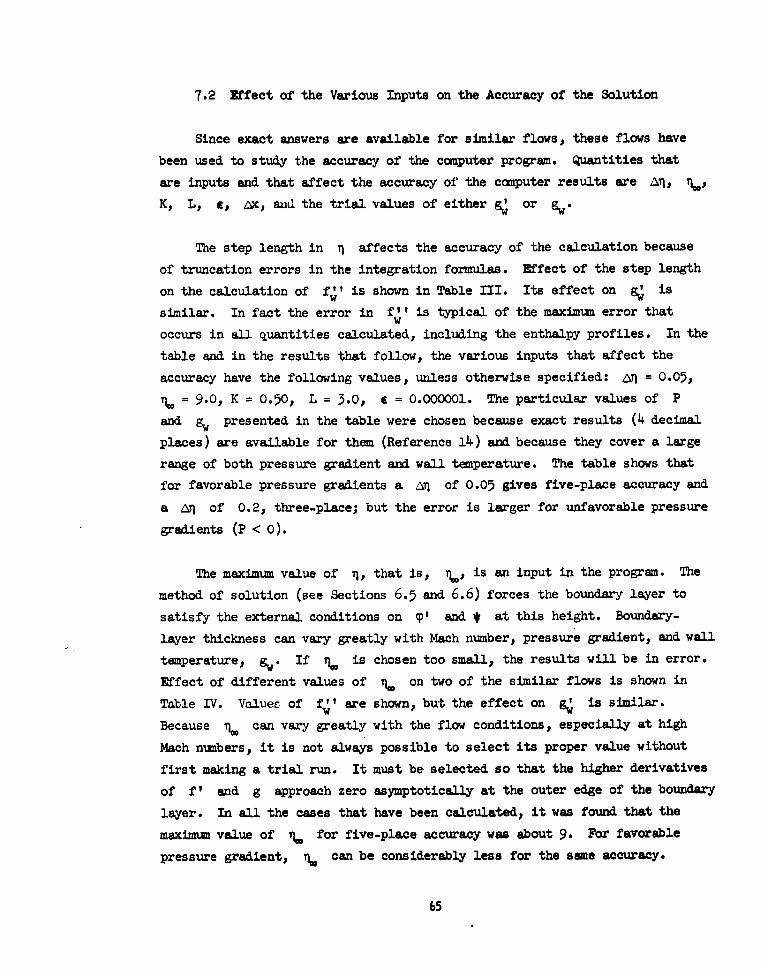
7.2 Effect of the Various Inputs on the Accuracy of the Solution
Since exact answers are available for similar flows, these flows have
been used to study the accuracy of± the computer program. Quantities that
are inputs and that affect the accuracy of the computer results are Al, ,
K, L, c, Ax, mad the trial values of either g or gw"
The step length in il affects the accuracy of the calculation because
of truncation errors in the integration formulas. Effect of the step length
on the calculation of fw' is shown in Table III. Its effect on g is
similar. In fact the error in f' is typical of the maximum error thatwoccurs in all quantities calculated, including the enthalpy profiles. In the
table and in the results that follow, the various inputs that affect the
accuracy have the following values, unless otherwise specified: nTI = 0.05,
r6 = 9.0, K = 0.50, L = 3.0, t = 0.000001. The particular values of P
and gw presented in the table were chosen because exact results (4 decimal
places) are available for them (Reference 14) and because they cover a large
range of both pressure gradient and wall temperature. The table shows that
for favorable pressure gradients a Aq of 0.05 gives five-place accuracy and
a an of 0.2, three-place; but the error is larger for unfavorable pressure
gradients (P < 0).
The maximum value of q, that is, %, is an input in the program. The
method of solution (see Sections 6.5 and 6.6) forces the boundary layer to
satisfy the external conditions on q' and * at this height. Boundary-
layer thickness can vary greatly with Mach number, pressure gradient, and wall
temperature, gw" If % is chosen too small, the results will be in error.
Effect of different values of % on two of the similar flows is shown in
Table IV. Values of f'I are shown, but the effect on g; is similar.
Because % can vary greatly with the flow conditions, especially at high
Mach numbers, it is not always possible to select its proper value without
first making a trial run. It must be selected so that the higher derivatives
of f' and g approach zero asymptotically at the outer edge of the boundary
layer. In all the cases that have been calculated, it was found that the
maximum value of r for five-place accuracy was about 9. For favorable
pressure gradient, % can be considerably less for the same accuracy.
65
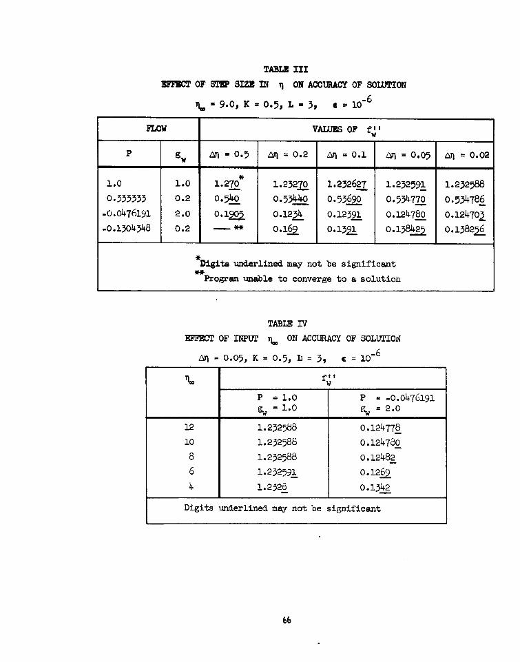
TABLE III
EFFCT OF STE SIZE IN I ON ACCURACY OF SOLUTION
S=9.0, K =O.5 L=3, = 10- 6
FLOW VALUES OF f' I
P w an = 0.5 I = 0.2 A'= 0.1 A = 0.05 n = 0.02
1.0 1.0 1.270 1.23270 1.232627 1.232591 1.232588
0.33333 0.2 O.540 0.5 3440 0.55690 0.534770 0.534786
-0.0476191 2.0 0.12M 0.1234 0.12391 0.124780 o.124703
-0.13o4348 0.2 - O.129 0.1391 0.1384g o.138226
*Digits underlined may not be significantProgram unable to converge to a solution
TABLE IV
EFFECT OF INPUT r6 ON ACCURACY OF SOLUTION
Af= 0.05, K = 0.5, L = 3, e = 10 - 6
w
P = 1.0 P = -0.0476191w = 1.0 gw = 2.0
12 1.232588 0.124778
10 1.232588 0.124780
8 1.252588 0.12482
6 1.232591 0.1269
4 1.2328 o.1342
Digits underlined may not be significant
66
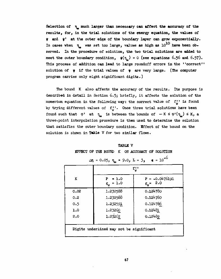
Selection of % much larger than necessary can affect the accuracy of the
results, for, in the trial solutions of the energy equation, the values of
* and ,' at the outer edge of the boundary layer can grow exponentially.
In cases when % was set too large, values as high as 1010 have been ob-
served. In the procedure of solution, the two trial solutions are added to
meet the outer boundary condition, *(C) = 0 (see equations 6.56 and 6.57).
This process of addition can lead to large roundoff errors in the "correct"
solution of * if the trial values of * are very large. (The computer
program carries only eight significant digits.)
The bound K also affects the accuracy of the results. Its purpose is
described in detail in Section 6.5; briefly, it affects the solution of the
momentum equation in the following way: the correct value of f'' is foundw
by trying different values of f"'. Once three trial solutions have beenw
found such that cp' at T is between the bounds of -K S qI'(TI) 9 K, a
three-point interpolation procedure is then used to determine the solution
that satisfies the outer boundary condition. Effect of the bound on the
solution is shown in Table V for two similar flows.
TABLE V
EFFECT OF THE BOUND K ON ACCURACY OF SOLUTION
LO0.05, =9.0, L = 3, 6 = 10-6
fw
K P = 1.0 P = -0.0476191%, = 1.o 02.0
0.02 1.232588 0.124780
0.2 1.232588 0.124780
0.5 1.232591 0.124786
1.0 1.2326o 0.12481
2.0 1.23262 0.12482
Digits underlined may not be significant
67
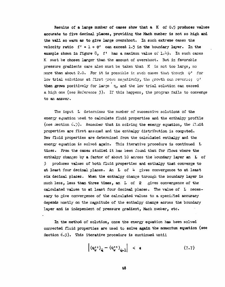
Results of a large number of cases show that a K of 0.5 produces values
accurate to five decimal places, providing the Mach number is not so high and
the wall so warm as to give large overshoot. In such extreme cases the
velocity ratio V = 1 + CP' can exceed 1.5 in the boundary layer. In the
example shown in figure 8, V has a maximum value of 1.49. In such cases
K must be chosen larger than the amount of overshoot. But in favorable
pressure gradients care also must be taken that K is not too large, no
more than about 2.0. For it is possible in such cases that though 9' for
low trial solutions at first :rows negatively, the growth can reverze; c?'
then grows positively for large , and the low trial solution can exceed
a high one (see Reference 3). If this happens, the program fails to converge
to an answer.
The input L determines the number of successive solutions of the
energy equation used to calculate fluid properties and the enthalpy profile
(see Section 6.9). Remember that in solving the energy equation, the f.uid
properties are first assumed and the enthalpy distribution is computed.
New fluid properties are determined from the calculated enthalpy and the
energy equation is solved again. This iterative procedure is continued L
times. From the cases studied it has been found that for flows where the
enthalpy changes by a factor of about 10 across the boundary layer an L of
3 produces values of both fluid properties and enthalpy that converge to
at least four decimal places. An L of 4 gives convergence to at least
six decimal places. When the enthalpy change through the boundary layer is
much less, less then three times, an L of 2 gives convergence of the
calculated values to at least four decimal places. The value of L neces-
sary to give convergence of the calculated values to a specified accuracy
depends mostly on the magnitude of the enthalpy change across the boundary
layer and is independent of pressure gradient, Mach number, etc.
In the method of solution, once the energy equation has been solved
corrected fluid properties are used to solve again the momentum equation (see
Section 6.9). This iterative procedure is continued until
(C") -w (Iw')QlI < a (7.7)
68
where a is an input and Q is a count of successive calculations of the
momentum equation. Againp as with L, the number of times, Q + 1, that the
momentum equation has to be solved in order to satisfy eq.(7.7), depends
mostly on the enthalpy change across the boundary layer and appears to be
independent of pressure gradient, Mach number, etc. Variation of Q with c
is shown in Table VI.
TABLE VINUMB OF SUCCESSIVE CALCULATIONS (Q + i) OF MOMEMM EQUATION
NECESSARY TO SATISFY ACCURACY REQUIREMENT
(P'14- (C"< a
Enthalpy Change
Across =106 a = lO 5 a 10 4 4 10 3
Boundary Layer
Approximately
10 Times 5 3 3 2
3 Times or Less 3 2 1 1
The effect of step length in x on the solution appears to-be identical
to that reported by the authors in References 2 and 3 for the incompressible
boundary layer. The details will not be repeated here; but, briefly, not
only must the size of A x be considered in selecting the spacing in the
x-direction, but also the quantity x/c. The latter appears in the terms
containing the x-derivatives in the following way. From the momentum equation
the term containing the x-derivative of (' is replaced by a finite-difference
term of the form
-? x, x @
AXx
69
As a x approaches zero _' approaches zero in an exact solution; but in
the computer program roundoff errors exist and, furthermore, these errors are
multiplied by the quantity x/A x. Therefore as A x approaches zero the
error in the solution is not necessarily decreased. This type of roundoff
error is observed as A x becomes small in the present method. It does not
occur for values of x/A x less than about 25. The maximum error that has
been observed is one in the fifth significant digit for x/a x %- 25. The
error grows as x/A x becomes larger. Of course, this roundoff error is a
function of the number of significant digitst eight, that are carried in the
computer program and is not inherent in the method of solution. It can be
reduced by using "double precision" routines, that is, sixteen significant
digits would be carried instead of the present eight. In all of the calcu-
lations presented in this report A x was selected so that the quantity
x/A x was less than 25. Therefore it is believed that the results are free
of this type of roundoff error.
In particular cases care in selecting two of the other input quantities
is necessary to prevent erroneous results. If gw is known, two trial values
of g must be input; or if g is known, then two trial values of g.,
must be input. In the method of solution these two trial values are used to
obtain two solutions of the energy equation (see Section 6.6). Then, because
the equation is linear, the correct solution is found by combining the two
solutions to meet the outer boundary conditions. If the trial values at thewall are far from the correct solution, the trial values of 4 and 4' can
become very large near the outer edge of the boundary layer. This is the
same phenomenon that occurs when . is selected too large, and that is dis-
cussed above. In one example when solving for g which had a correct value
of approximately 0.4, trial values of 0.0 and 1.0 were input. At the
the outer edge of the boundary layer they led to values of * of around
-109 and +10 respectively. When the two solutions were combined, in order
to satisfy the outer boundary condition (see equations 6.56 and 6.57), the
large trial values led to roundoff errors in the second significant digit
of *. This roundoff error can be eliminated by selecting trial values of
&; (or gw) near to the correct value, within one significant digit.
Selection is done by either experience or a trial run. The magnitude of the
roundoff error can be easily seen by inspecting values of # and *' near T.
7C
7.3 Flow on a Flat Plate with Variable Temperature
Charman and Rubesin developed a method for calculatlzg exactly the com-
pressible laminar boundary layer on a flat plate with variable wall tempera-
ture (Reference 15). The method requires that the surface temperature distri-
bution be expressible as a polynomial in surface distance, that the viscosity
varies linearly with temperature through the boundary layer, and that the
Prandtl number be constant. One of the examples presented by Chapan and
Rubesin was calculated by the present method with the same assumptions for
fluid properties. The distribution of surface temperature is given by
T Tad TwT - - (0.25 - 0.83 x + 0.33 (7.8)T_-T_= _Tx)e. e e
where Tad/Te = 1 + 0.169 is the wall recovery temperature and Te is
the temperature at the edge of the boundary layer. Since constant c. is
assumed the wall enthalpy distribution has the same form as the temperature.
The external flow has a Mach number of 3.0. Results of the two calculations
are coupared in figure 9 in the form of
qx ()- --
versus x. The latter quantity is the parameter used by Chapman and Rubesln.
Greatest disagreement between the two methods is 5 in the fourth significant
digit. Furthermore, this difference is consistent for the whole length of
flow; the values calculated by the present method are (0.4 . 0.1) percent
legs than the values calculated by Chapman and Rubesin. In the present
method inputs were selected in such a way that the calculation was accurate
to five decimal places. In using the method of Chapman and Rubesin the cal-
culation depended on parameters given to four figures in Reference 15.
Therefore the two calculations might be expected to agree to at least four
decimal places. But Chapman and Rubesin do not specifically state that all
four digits presented are significant. The value of recovery factor they
calculated is presented to only three figures, a recovery factor - 0.845.
This affects the values of the other quantities - temperature and heat transfer-
71
calculated by their method. Recovery factor calculated by the present method
for the flow is 0.8475. The ratio of recovery temperature calculated by the
present method to that by Chapa and Rubesin is 1.0018.
7.4 Effect of Fluid-Property Laws on Recovery Factor
Effect of the various fluid-property laws on recovery factor was studied
for flow over a flat plate and flow over a cone at Mach numbers fron 1.0 to
10.0. Recovery factor rf had its usual definition
Ta,=h ad + rfY- (-0Te e
Relation (7.10) is exact only if cp is constant. Fluid-property laws studied
included: first, a viscosity proportional to temperature and an arbitrary but
constant Prandtl number, and second, the "exact" property laws of Cohen (see
Section 6.3). The assumption of viscosity proportional to temperature in the
boundary layer gives a value of C = pP/Pepe of 1.0, since density is in-
versely proportional to temperature across the boundary layer. Recovery factor
versus Mach number is shown in figure lOa for the various laws. Cohen's re-
lations are not used below a Mach number of 2.0 because they are not valid
below that Mach number for the altitude assumed, 50,000 ft. They are not
valid for h/href < 0.0152, where href is Cohen's reference enthalpy,
2.119 x 108 ft 2 /sec 2 . The assumptions of viscosity proportional to temperature,
C = 1.0, and a constant Prandtl number of 0.72, which are often used in boundary.
layer work, give recovery factors that are within 3.3 percent of those calcu-
lated with the more nearly exact properties. The calculated recovery factors
for a cone are identical to those for the flat plate with indentical boundary
conditions.
Variation of the calculated recovery factors with Prandtl number at the
wall is shown in figure lOb. The approximate relation that is often assumed
in boundary-layer theory
rf - (7.11)
is also shown.
72
7.5 Comparison of Present Method with that of Flgge-Lotz
and Blottner
Recently Fltgge-Lotz and Blottner developed an implicit finite-difference
method for calculating the compressible laminar boundary layer (Reference 6).
Fluid-property relations that were used included an arbitrary but constant
Prandtl number and one of two relations for viscosity. Either Sutherland's
viscosity law or a viscosity that varied linearly with temperature was used,
and examples for both are given in Reference 6. Since, as of now, the present
method is programed to use either Cohen's "exact" relation for viscosity or
a linear variation with temperature, results of the two methods can be compared
directly only for the examples in Reference 6 that use the linear viscosity
law. These examples consist of a flat plate at Mach number 3.J with an in-
sulated wall and with a heated wall such that Tw/TMd = 2.0. Because the
boundary conditions are independent of x. the flows can also be calculated
by similar-flow methods. Flffgge-Lotz and Blottner compare their results with
the similar solution of Low (Reference 16). The results of the present method
are compared with the same method.
The shear parameter f' calculated by the present method agrees withw
that calculated by Low's method within the accuracy with which his method can
be used. His method uses parameters presented to only four decimal places.
For the heated plate Low's method gives f' = 0.33205 as compared to
0.332057 obtained by the present method. FlUgge-Lotz and Blottner compare
their results with Low's in graphical form, and it appears that values of
fw" agree to at least four decimal places a short distance downstream of the
start of the calculation. At the start the agreement between the two methods
is not so close. In the method of Flgge-Lotz and Blottner the form of the
equation is singular at x = 0, and the calculation must be started at some
point downstream of x = 0. Furthermore, the initial profile must be specified
at this starting point. FlUgge-Lotz and Blottner used the similar profile of
Low to get started, and they state in Reference 6 "Since the initial profiles
are only accurate to four decimal places, there are initially errors in the
boundary-layer calculations and characteristics. These errors appear to de-
crease as the computations proceed.''
73
7.5 Comparison of Present Method with that of Flffgge-Lotz
and Blottner
Recently Flgge-Lotz and Blottner developed an implicit finite-difference
method for calculating the compressible laminar boundary layer (Reference 6).
Fluid-property relations that were used included an arbitrary but constant
Prandtl number and one of two relations for viscosity. Either Sutherland's
viscosity law or a viscosity that varied linearly with temperature was used,
and examples for both are given in Reference 6. Since, as of now, the present
method is programed to use either Cohen's "exact" relation for viscosity or
a lin.ar variation with temperaturej results of the two methods can be compared
directly only for the examples in Reference 6 that use the linear viscosity
law. These examples consist of a flat plate at Mach number 3.0 with an in-
sulated wall and with a heated wall such that Tw/Tad = 2.0. Because the
boundary conditions are independent of x, the flows can also be calculated
by similar-flow methods. Flgge-Lotz and Blottner compare their results with
the similar solution of Low (Reference 16). The results of the present method
are compared with the same method.
The shear parameter f"' calculated by the present method agrees with
that calculated by Low's method within the accuracy with which his method can
be used. His method uses parameters presented to only four decimal places.
For the heated plate Low's method gives f,' = 0.33205 as compared to
0.332057 obtained by the present method. Flgge-Lotz and Blottner compare
their results with Low's in graphical form, and it appears that values of
f" agree to at least four decimal places a short distance downstream of thewstart of the calculation. At the start the agreement between the two methods
is not so close. In the method of Fltfgge-Lotz and Blottner the form of the
equation is singular at z = 0, and the calculation must be started at some
point downstream of x - 0. Furthermore, the initial profile must be specified
at this starting point. Flgge-Lotz and Blottner used the similar profile of
Low to get started, and they state in Reference 6 "Since the initial profiles
are only accurate to four decimal places, there are initially errors in the
boundary-layer calculations and characteristics. These errors appear to de-
crease as the computations proceed."
73
The agreement of heat-transfer values calculated by the present method
with those of Low's similar method is not so good as that for the shear para-
meter. For the heated plate at Mach 3.0, the present method gave a value of
of -0.29416 as compared to -0.29367 obtained from Low's parameters.
Since Low presents his data to four decimal places, better agreement might be
expected. The disagreement may be due to the difference in the recovery fac-
tor calculated and used by Low, rf = 0.8477. and that calculated by the
present method, 0.84746. Fltgge-Lotz and Blottner also compare their heat-
transfer values with Low's values calculated for the same flow. Close obser-
vation of their graphs at a point downstream of the initial x-station appears
to show that their results are around 0.2 percent higher than Low's (see
figures 6(b) and 7(b) of Reference 6). This is. about the sae percentage
difference that appears between the present method and Low's, that is,
Present method g;= 1.002
Low's I
Velocity and enthalpy profiles as calculated by the three methods - Low,
FlUgge-Lotz and Blottner, and present - agree to three decimal places at the
one station, x = 1.10, where data exist so that such a comparison could be
made. This is within the accuracy with which the profiles are presented in
Reference 6.
7.6 Comparison of Heat Transfer Calculated by the Present
Method with that Measured on a Circular Cylinder
Few experimental data on compressible boundary layers are available for
comparison with the prediction of theories. Exceptions are a few heat-trans-
fer data. Reference 17 presents experimental data on heat transfer measured
on circular cylinders with their axes normal to the flow at several Mach
numbers. Comparison of the measured heat transfer with that calculated by the
present method is shown in figure 11. The external velocity and onset flow
conditions used in the calculation were obtained from Reference 17. The ex-
perimental temperatures were so low that the relations for fluid properties
given by Cohen (see Section 6.3) are invalid. Therefore, the simple assuzp-
tions of constant Prandtl number (0.72) and a viscosity proportional to
temperature through the boundary layer were assumed.
74
As discussed by the authors of Reference 17, the magnitude of the experi-
mental error is not known; but it may be as great as the difference between
the calculated and measured results in figure 11. They point out that the
experimental data at M = 4.15 are known to include experimental error not
present at the other Mach numbers, and, furthermore, that the error in
instrumentation tends to increase the indicated heat transfer rearward of 400.
They also state that "for a Z 900 the accuracy of all the data becomes
questionable because of the very small convective heat rates compared with
radiation and other sources of error." To avoid confusion with experimental
points, calculated points are not indicated in the figure, but the step size
was 5o except near the stagnation pointwhere step lengths of 1i were used.
Smaller steps were used here in order to converge on the heat-transfer rate
at the stagnation point. Values calculated are believed to be accurate to
three decimal places. Experimental data were obtained at gw '- 1.0, 0.8,
and 0.7. The calculated curves shown are for g = 0.8, but calculations at
the other two enthalpies were very similar. A gw of 0.70 gives values of
[9./(,d- gw)]/[gw/(gd- 9w)]st&1 that are from 0.7 to 1.2 percent higher
than those shown.
7.7 Boundary Layer in an Axisymmetric Convergent-Divergent
Rocket Nozzle
As an example of internal axisymmetric flow the boundary layer inside
a rocket nozzle was calculated. The flow involves both large pressure
gradients and heat transfer. It is similar to the flow calculated by C. B.
Cohen and E. Reshotko in Reference 18, but an exact comparison between the two
calculations can not be made because there is insufficient information on the
flow properties and the nozzle dimensions of Reference 18. Radius, surface
distance, and the velocity and Mach number at the center of the nozzle are
plotted in figure 12 against the axial distance. These local flow conditions
were obtained by means of simple one-dimensional flow relations. Stagnation
pressure is assumed to be 500 pounds per square inch and stagnation tempera-
ture as 40000R, which leads to a total enthalpy He = 27.246 x 106 ft 2 /sec 2 .
The nozzle wall is assumed cooled to a uniform temperature of 800*R, which
corresponds to an enthalpy ratio of gw = 0.17625.
75
Results of the calculation are presented in figure 13. The skin-friction
coefficient cf , defined by equation (6.115), and the ratio of Stanton number
to skin friction coefficient, defined by equations (6.120) and (6.121), are
shown. Calculations denoted by ''exact properties'' were obtained by using
the relations of N.B.Cohen described in Section 6.3. A calculation was also
made by using the simple assumptions of constant Prandtl number and viscosity
proportional to local enthalpy. Because of the high enthalpies involved, a
Prandtl number of 0.78 was chosen. Figure 13 shows that these simple assump-
tions for fluid properties lead to results that seriously overestimate both
skin friction and heat transfer at the higher Mach number. At the lower Mach
numbers, the effect is reversed, that is, the simple assumptions gave lower
skin friction and heat transfer than those calculated for exact properties.
This study and those in previous sections indicate that the exact-property62 2
relations should be used if the local enthalpy exceeds 4 x 10 ft2/sec
Stagnation-point flow is assumed at the start of the flow (x = 0).
Because ue = 0, here, the skin friction coefficient cf is singular and,
of course, can not be presented at the stagnation point in figure 13. The
shear parameter f" and also the gradient of g at the wall, g , are
finite here and are
f= 0.38084 ; g = 0.16523 for exact properties
wf'w '= 0.73507 ; = 0.58177 for C = 1.0, Pr =0.78
7.8 Boundary Layer on a Spherically Blunted Cone at Mach
Numbers of 3.0 and 9.0
Boundary layers were calculated on a reentry-type body that consists of
a 15* half-angle cone blunted with a spherical nose. The conical and spherical
surfaces join in such a way that there is no discontinuity in body slope. The
velocity distribution outside the boundary layer was calculated by a computer
program that consists of (1) a solution of the blunt-body problem from the
stagnation point to a point past the sonic point and (2) a solution by the
method of characteristics in the supersonic flow region. The method of
76
characteristics is started just aft of the sonic point by using local veloci-
ties and pressures given by the blunt-body solution as an initial boundary
condition. Variation of the inviscid velocity and Mach number with axial
distance is shown in figure 14. Surface distance and local radius are also
shown. Though the velocity varies smoothly in going from the blunt-body
solution to the characteristics solution, there is a large change in velocity
gradient, due/dx, just aft of the point where the change in methods occurs,
x = 0.9. This results in large changes in the parameter P = (x/ue)(due/dx)
just aft of this point, which produces large changes in the calculated values,
as will be seen below.
Boundary layers on the body were calculated at the two speeds, M = 3.0
amd 9.0, at three altitudes, 50,000, 100,000 and 250,000 ft., for three body
temperatures. Results for M = 3.0 are shown in figure 15 (a, b, c). Results
are independent of altitude to three decimal places; therefore,only the 50,000-
ft values are shown. The reason that the effect of altitude is found to be
negligible is that there is only a small change in total enthalpy with altitude.
Total enthalpy is given in Table VII for the three altitudes. Also, the
reference velocity at that is used to nondimesionalize the velocity ue is
given. The velocity at is the velocity of sound at free-stream stagnation
conditions. The total enthalpy of about 6.6 x 106 ft /sec 2 at the lower
altitudes corresponds to a total temperature of about 1090eR. The three body
temperatures presented are: gw = 0.357, which gives a body temperature equal
to about the static temperature of the onset flow; gw - 0.458, which gives a
wall temperature equal to about 500 F; and an adiabatic wall, which is calculated
by setting g = 0. Variation of the skin-friction coefficient cf and ratio
of Stanton number to the skin friction coefficient St/cf with surface distance
are shown for the flows when U. is specified. When an adiabatic wall ( = 0)
is specified, cf and 9 are shown. To further investigate the effect of
fluid-property laws on the solution, the flows were calculated twice, once
with the ''exact fluid properties'' of Cohen (Section 6.3), and again with the
simple assumptions of constant Prandtl nunber and a linear viscosity law. It
is seen that the simple assumptions greatly overestimate the skin friction and
heat transfer (figure 15(a, b)) and, in the adiabatic wall case, the surface
temperature (figure 15c). For the results with exact properties the figures
show a "bump" in c. just aft of x = 0.90. This is at the point, mentioned
77
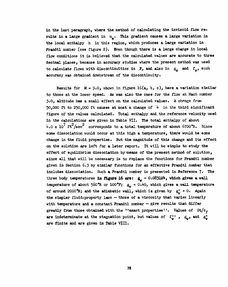
in the last paragraph, where the method of calculating the inviscid flow re-
sults in a large gradient in u e . This gradient causes a large variation in
the local enthalpy h in this region, which produces a large variation in
Prandtl number (see figure 2). Even though there is a large change in local
flow conditions it is believed that the calculated values are accurate to three
decimal places, because in accuracy studies where the present method was used
to calculate flows with discontinuities in P, and also in gw and fw' such
accuracy was obtained downstream of the discontinuity.
Results for M = 9.0, shown in figure 16 (a, b, c), have a variation similar
to those at the lower speed. As was also the case for the flow at Mach number
3.0, altitude has a small effect on the calculated values. A change from
50,000 ft to 250,000 ft causes at most a change of 4 in the third simnificant
figure of the values calculated. Total enthalpy and the reference velocity used
in the calculations are given in Table VII. The total enthalpy of about
4.0 x 107 ft2/sec2 corresponds to a total temperature of about 6700R. Since
some dissociation would occur at this high a temperature, there would be some
change in the fluid properties. But the magnitude of this change and its effect
on the solution are left for a later report. It will be simple to study the
effect of equilibrium dissociation by-means of the present method of solution,
since all that will be necessary is to replace the functions for Prandtl number
given in Section 6.3 by similar functions for an effective Prandtl number that
includes dissociation. Such a Prandtl number is presented in Reference 7. The
three body temperatures in figue 16 are: gw = 0.083124, which gives a wall
temperature of about 560*R or 100*F; gw = 0.40, which gives a wall temperature
of around 2000*R; and the adiabatic wall, which is given by g = 0. Again
the simpler fluid-property laws - those of a viscosity that varies linearly
with temperature and a constant Prandtl number - give results that differ
greatly from those obtained with the "exact properties". Values of St/cf
are indeterminate at the stagnation point, but values of fw' , gw,, and
are finite and are given in Table VIII.
78
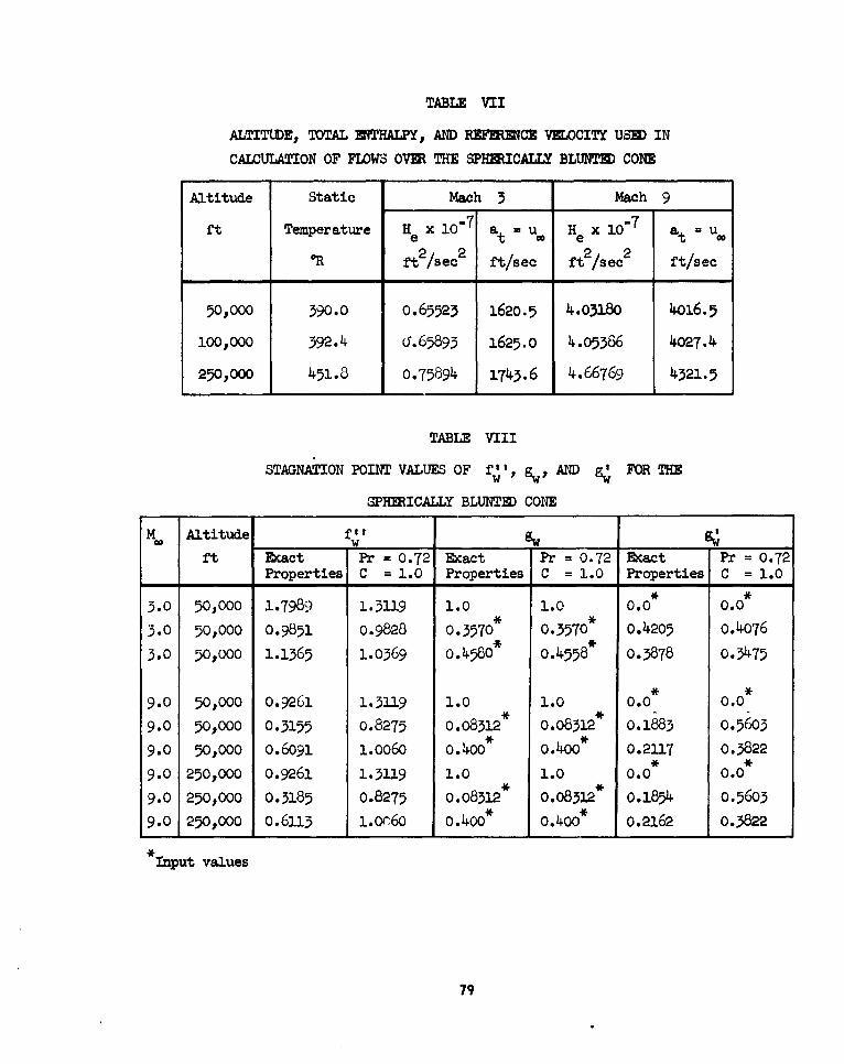
TABLE VII
ALTITUDE, TOTAL ENTHALPYp AND REFNCE VE.OCITf USED IN
CALCULATION OF FLOWS OVE THE SPHERICALLY BLUNTED CONE
Altitude Static Mach 3 Mach 9
ft Temperature H x10 7 at = u He X 10-7 at = u
Rftsec ft/sec ft 2 /sec ft/sec
50,000 390.0 0.65523 1620.5 4.03180 4016.5
100,000 392.4 (J.65893 1625.0 4.05386 4027.4
250,000 451.8 0.75894 1743.6 4.66769 4321.5
TABLE VIII
STAGNATION POINT VALUES OF f'. gw' AND FOR THE
SPHERICALLY BLUNTED CONE
M Altitude fi' _g
ft Exact Pr = 0.72 Exact Pr = 0.72 Exact Pr = 0.72Properties C = 1.0 Properties C = 1.0 Properties C = 1.0
3.0 50,000 1.7989 1.3119 1.0 1.0 0.0 0.0
3.0 50,000 0.9851 0.9828 0.3570* 0.3570* 0.4205 0.4076
3.0 50,000 1.1365 1.0369 0.4580* 0.4558* 0.3878 0.3475
9.0 50,000 0.9261 1.3319 1.0 1.0 0.0 0.0
9.0 50,000 0.3155 0.8275 0.08312" 0.08312* 0.1883 o.5(439.0 50,000 0.6091 1.OO60 o.4oo* 0.400* 0.2117 0.3822
9.0 250,000 0.9261 1.3119 1.0 1.0 0.0 0.0* *
9.0 250,000 0.3185 0.8275 0.08312 o.o8312 o.1854 0.5603
9.0 250,000 0.6113 i.0c60 0.400* 0.400* 0.2162 0.3822
*Input values
79
7.9 Transverse Curvature Effect in Axially Symmetric Flow
In all the examples presented so far, the transverse curvature terms have
been neglected. These terms become of importance when the boundary layer has
a thickness of about the same magnitude as the body radius. There are two of
these terms: the first term., which includes T, on the right-hand side of
both the momentum equation (6.35) and the energy equation (6.46) and the termP+ 1
that contains N = = + R in both equations. The transverse curvature
parameter T is defined by (6.32) and the radius parameter R by (6.33b).
Transverse curvature effects were investigated by Probstein and Elliott,
Reference 19. The study was restricted to similar flow and essentially ex-
panded the stream function f and the enthalpy function g in a power
series in E, where
Ve Cos r 1/2
0 0
8 cos a (7.12)r
That is,
f(, ) fo(n) + t fl(n) + E2 f2(7 ) ...
-Z fj(n) (7.13)j=o
and there is a similar function for enthalpy. The expansion parameter was
assumed to be small with respect to unity. Substituting their asymptotic
expansions into the momentum and energy equations, and equating to zero all
terms with the same power in g, Probstein and ELliot obtained a double
infinity of ordinary differential equations. They found all these equations
except the zeroth order momentum equation to be linear, because a Pr = 1.0
and a viscosity proportional to temperature had been assumed. They obtained
solutions of the zeroth- and first-order equations. They forced the equations
to be similar, that is, independent of x, by assuming g to be constant.
As discussed by them, this assumption requires that the boundary-layer thick-
ness be directly proportional to the body radius. They present solutions for
80
only two types of bodies - a cone and a cylinder with axes aligned with the
flow. Their assumption of similarity - that 8* varies as the body radius -
is a poor approximation for these two bodies, for in reality the thickness
grows nearly parabolically with x, as
The present method was used to calculate the boundary layer on the sane
two types of bodies. Assumptions on the fluid properties are the same as
those used by Probstein and Elliott. Results are presented in terms of the
parameters used by them,
ro0 71 f ' - (f' ')T = 0 (-4x (7.it).
w T=0
for the cylinder, and
fit - (fZ')T =0( 15tan f (7.15)
(f")=
for the cone, where Re = uex/ve ; a is the angle between the normal to sur-
face and the radius, but is also the half angle of the cone here; and the sub-
script T = 0 denotes the solution with no transverse curvature effect. For
the cylinder the radius parameter R is zero, and for the cone it is given
exactly by (6-33b)x dro
R = - -(6.33b)i1+ Tw -7-dr
0
since cos a is constant. Calculations for a large range in Reynolds numbers,
up to 107, at Mach numbers from 1.0 to 10.0, wall enthalpy ratios hw/he from
1.0 to 10.0, and, for the case of cone flow, a of from 5* to 20* showed that
the parameters (7.14) and (7.15) asymptotically approached a constant as the
solution proceeded downstream. It was found that the asymptotes depended
mostly only on Mach number and body temperature and were nearly independent
of Reynolds number, body radius, and, in the case of the cone, the cone angle.
Sample solutions are shown in figures 17 and 18 for a cylinder and cone,
respectively. Probstein and Elliott's solutions for the same flows are indi-
cated in the figures and give values of the parameters plotted that are
81
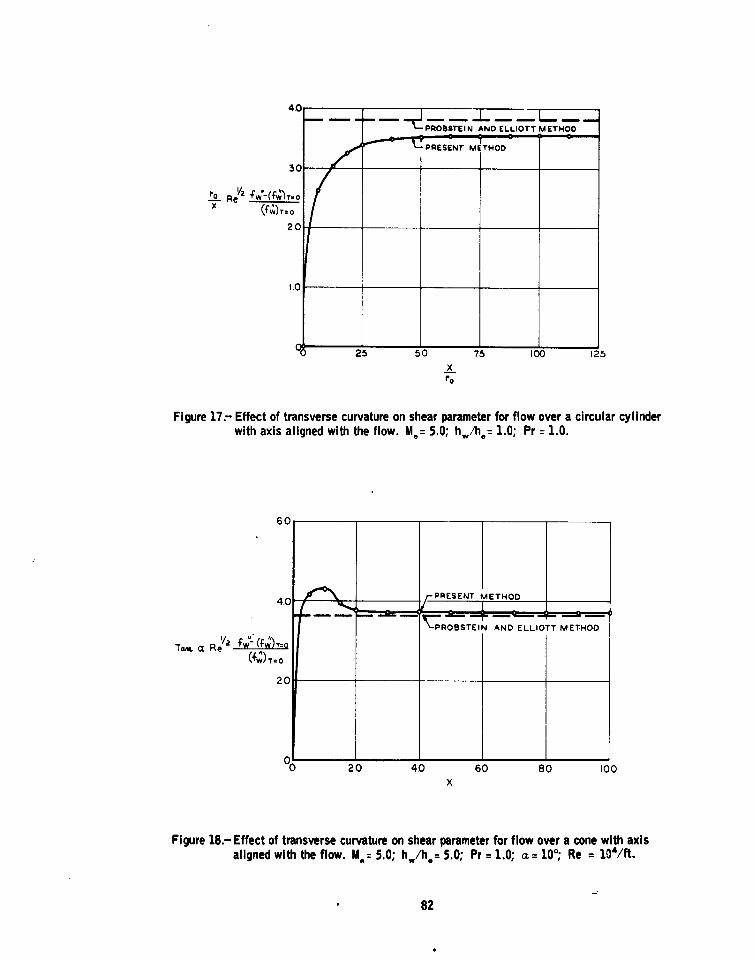
40
eOSTEIN AND ELLIOTT M ETHOD
30C
PO Re/ 2 wV-(fmoX (f )T=O
005 50 75 100 125
xPo
Figure 17- Effect of transverse curvature on shear parameter for flow over a circular cylinderwith axis aligned with the flow. M.= 5.0; hv/h.= 1.0; Pr =1.0.
60
4. PRESENT METHOD
-ROBSTEIN AND ELLIOTT METHOD'/2 'fw" ("fw)'ro
Ta.t a Re/'
20
0 20 40 60 80 100X
Figure 18.- Effect of transverse curvature on shear parameter for flow over a cone with axisaligned with the flow. M. = 5.0; hw/h.= 5.0; Pr = 1.0; a= 100; Re 104/ft.
82
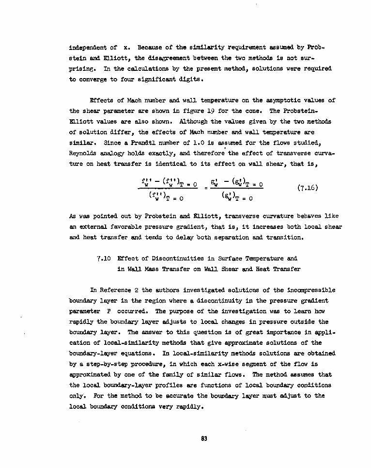
independent of x. Because of the similarity requirement assumed by Pr~b-
stein and Elliottl the disagreement between the two methods is not sur-
prising. In the calculations by the present method, solutions were required
to converge to four significant digits.
Effects of Mach number and wall temperature on the asymptotic values of
the shear parameter are shown in figure 19 for the cone. The Probstein-
Elliott values are also shown. Although the values given by the two methods
of solution differ, the effects of Mach number and wall temperature are
similar. Since a Prandtl number of 1.0 is assumed for the flows studied,
Reynolds analogy holds exactly, and therefore the effect of transverse curva-
ture on heat transfer is identical to its effect on wall shear, that is,
O =0 9; (7.16)
w o = 0
As was pointed out by Probstein and Elliott, transverse curvature behaves like
an external favorable pressure gradient, that is, it increases both local shear
and heat transfer and tends to delay both separation and transition.
7.10 Effect of Discontinuities in Surface Temperature and
in Wall Mass Transfer on Wall Shear and Heat Transfer
In Reference 2 the authors investigated solutions of the incompressible
boundary layer in the region where a discontinuity in the pressure gradient
parameter P occurred. The purpose of the investigation was to learn how
rapidly the boundary layer adjusts to local changes in pressure outside the
boundary layer. The answer to this question is of great importance in appli-
cation of local-similarity methods that give approximate solutions of the
boundary-layer equations. In local-similarity methods solutions are obtained
by a step-by-step procedure, in which each x-wise segnent of the flow is
approximated by one of the family of similar flows. The method assumes that
the local boundary-layer profiles are functions of local boundary conditions
only. For the method to be accurate the boundary layer must adjust to the
local boundary conditions very rapidly.
83
In the investigation of the incompressible boundary lae in the region
of a discontinuity in P, it was found that this adjustment to local boundary
conditions was surprisingly slow (Reference 2). Study of the same adjust-
ment for compressible flow by means of the present method shows that it is
nearly identical to that found earlier for incompressible flow. Also, the
present method was used to find how rapidly the boundary layer adjusted to
discontinuities both in wall temperature and in mass transfer at the surface
for supersonic flow. These effects are presented in this Section.
First, the effect of discontinuities in wall temperature gw on a flat
plate at Mach number 3.0 are presented. Prandtl number is assumed to be 0.72.
The wall temperature gw is constant forward of x = 1.0 and then abruptly
changes to another value downstream of x = 1.0. Three values of the wall
temperature were studied: bw = had, giving a value of g = 0.90134;
hw = 2 had, giving gw = 1.80268; and hw = hep giving w = 0.35714 . In
figure 20a calculated values of g are shown for the flows when g. is
initially the adiabatic value and then abruptly changes to the higher or
lower traperature downstream of x = 1.0. For comparison, the calculated
values are also shown for the case when the plate is adiabatic for the whole
length of flow. The latter is a similar flow and therefore independent of x.
A positive value of 9; means that heat is being transferred to the surface;
a negative value means that heat is being transferred from the surface to the
air. The figure shows that g; abruptly changes just aft of the discor!-
tinuity in gw and slowly approaches an asymptotic value as the flow proceeds
downstream. This asymptotic value, which is indicated in the figure, is the
same as that which would be obtained by a similar solution using the local
boundary conditions downstream of the discontinuity. It is seen that the cal-
culated value of 9 overshoots the asymptotic value just downstream of the
discontinuity and slowly approaches the value from the opposite side from which
it started. That is, in figure 20a for the case when gw = 0.35714 downstream,
the calculated value of g at first greatly exceeds its asymptotic value and
then approaches it from above as the calculation proceeds downstream. Step
size in x used in the calculation was selected in such a way as to give cal-
culated values accurate to three decimal places downstream of the discontinuity.
Local similarity methods would give a constant value of g; for the whole
84
length of flow downstream of the discontinuity, and, furthermore, this value
would be the asymptotic value indicated in the figure.
Similar plots for flows where g is initially 0.35714 and 1.80268
and then abruptly changes to the other two values are shown in figures 20b
and 20c, respectively. The adjustmnent of g; to the local boundary condi-
tions is like that shown in figure 20a. As was the case in the adjustment
of fw" to local changes in P, the adjustment of 4 to the local value of
is surprisingly slow. Since flat-plate flow, P = 0, is assumed for the
flows shown in figure 20 (a, b, and c), the term containing p eP in the
mcnentum equation (6.37) drops out, and the calculated values of f, f', and
f' are independent of gw"
ftthalpy profiles for two of the flows with discontinuity in gw are
shown in figure 21. It is seen that the enthalpy values adjust to the local
boundary conditions more rapidly near the wall than they do at the outer edge
of the boundary layer. Asymptotic profiles for the two flows are also shown.
Discontinuities in mass transfer at the surface were also investigated.
Two external flows were studied. First flat-plate flow similar to that des-
cribed in the previous paragraphs.is assumed: P = 0.0, Me = 3.0, Pr = 0.72.
It is assumed that air is blowing out of the surface forward of x 1.0 in
such a way that fw is equal to a constant. Aft of x = 1.0 the surface
is impermeable. Although there is a discontinuity in the suction velocity vw
the stream function f. is a continuous function since it is an integral of
vw over x (see equation 6.16). Two different blowing quantities are assumed
forward of x = 1.0: fw = -0.5 and -0.1. The resulting variation of fw
downstream of the discontinuity in vw is shown in figure 22a. Effects of
the mass transfer and its discontinuity on the calculated values of f" and
gw are shown in figures 22b and 22c, respectively, for the case of an in-
sulated plate. It is seen that blowing decreases both f.' and S.
The effect of blowing cold air at the front of a nearly insulated plate
is shown in figure 23. The some blowing quantities used in the previous para-
graph arc assumed (figure 22a). The air blown from the surface is assumed to
85
have the same temperature as the free stream, h = he, giving a value ofV
= 0.35714 forward of x = 1.0. Aft of x = 1.0, the surface is solid
and has a temperature close to the adiabatic temperature. Effects of thc
blowing and its discontinuity on g; are shown in figure 23b. For com-
parison values of g; for the case of no blowing (fw = 0) are also plotted.
Since flat-plate flow (P = 0) is assumed, the term containing pe/ in the
momentum equation disappears, and the calculated values of f, f', and f"IW
are independent of gw" Therefore the variation of f" with x for thiswcase of blowing cold air on a hot plate is the same as that shown in figure
22b for the case of blowing on an insulated plate.
The opposite effect, that of blowing hot air at the front of a cold plate,
is shown in figure 24 . Three different blowing quantities are assumed forward
of x = 1.0: fw = - 0.1 - 0.5, and - 1.0. The first two of these are
identical to those used on the plates described in the two previous paragraphs
and shown in figure 22a. The blowing air is assumed to have a temperature
nearly equal to the adiabatic temperature, g. = 1.0. Downstream of blowing
(x > 1.0) the surface has a temperature equal to the static temperature out-
side the boundary layer. Again the variation of g; with distance is shown.
The effect of blowing on the velocity and enthalpy profiles for this flow is
shown in figure 25. The adjustment of the profiles to the discontinuities in
mass transfer and temperature is typical of that observed for all flows where
such discontinuities occurred.
The effect of blowing air out of the surface at the front of a body is
applicable to some forms of ablation cooling. In practice, when ablation
cooling is used, the body is usually blunt and thus the flow is initially like
that of a stagnation-point flow rather than the flat-plate flow that was
assumed in the preceding paragraphs. Therefore the effect of blowing has also
been studied on a body that is initially blunt. The flow is assumed to be
stagnation-point flow (P = 1.0) for x 9 1.0 and then to change abruptly to
a constant pressure flow (P = 0.0) for x > 1.0. This assumption of an
abrupt change from stagnation-point flow to constant-pressure flow would not
be a bad approximation to the flow over the reentry type body, a spherically
blunted cone, studied in Section 7.8 and shown in figure 14. The mass-trans-
fer distributions are assumed to be the sane as those studied in the flat-
86
plate flow. Also the onset flow is the same. Effect of the discontinuities
in P and vv on an insulated body is shown in figure 26. Variation of
the shear parameter fI with distance is shown in figure 26c and of thewall enthalpy gw with distance in figure 26d. Note that even though the
pressure gradient parameter P, the suction parameter fw' and the heat-
transfer parameter 8 are constants in the stagnation-point flow region,
x < 1.0, the wall enthalpy, and thus ft', change because of the variation in
ue . The effect of blowing cold air initially out of the blunt body is shown
in figure 27. Aft of the discontinuities in both P and vw, the surface is
assumed to have a temperature equal to the total temperature of the flow.
Adjustment of the velocity and enthalpy profile to the change in P, v , and
gw is shown in figure 28 for one of the mass-transfer distributions of
figure 27.
In conclusion, the study of discontinuities in the boundary conditions -
P, gw, and fw - shows surprisingly slow adjustment of the boundary layer to
these local conditions. It appears that local similarity methods give
erroneous results for flows where rapid variation in the external or wall
boundary condition occurs.
7.11 Concluding Statement
The large number of calculations and their comparison with other methods
and experiment establish the fact that the method is rapid, highly accurate,
and powerful. About 0.25 minutes of ccmputing time on the IBM 7090 computer
are required to calculate the velocity and enthalpy profiles at one station
accurate to four significant digit. Since a typical flow requires from 20
to 30 stations, computer time averages between 5 and 7 minutes for solving a
given problem. The method appears capable of solving any flow problem for
which the boundary-layer equations themselves remain valid. It is now being
extended to handle flows where dissociation (both equilibrium and nonequl-
librium) occurs. Also effects of both catalytic and noncatalytic walls will
be included.
8
87
APPEMDIX A
DEVELOPM7T OF THE BOUIDARY-LAYM EQUATIONS FOR COMPRE-S3BLE
LAIKAR FLOW INCLUDING THE EFFECT OF MANSVERSE CURVATURE
In this Anpendix the boundary-layer equations are developed for axially
symetric flow for the coordinate system of Section 6.1. The effects of
transverse curvature are included.
Continuity Equation
The continuity equation is
t + div(p V) = 0(Al)
The first term is of course zero for steady flow.
Before writing (Al) in the xy coordinate system, consider the general
orthogonal coordinates. Let
X, Y, Z, o.* any Cartesian coordinates
a V a2, a3" a* any orthogonal coordinates
Let the elements of length in the direction of increasing ci' 2 and a.
be h,?,. h 2 2, and h 3, respectively, so that
(d)2 = h2(d1)2 + h2(d )2 + h32 (d3)2 (A2)
The quantities h1 , h2 , and h3 are defined by
h ( )2 + ( +) +W 2lax5 a l 2 /az \
ax +2 az4'2 (F2 2
h 3 2 + +WJ jT
88
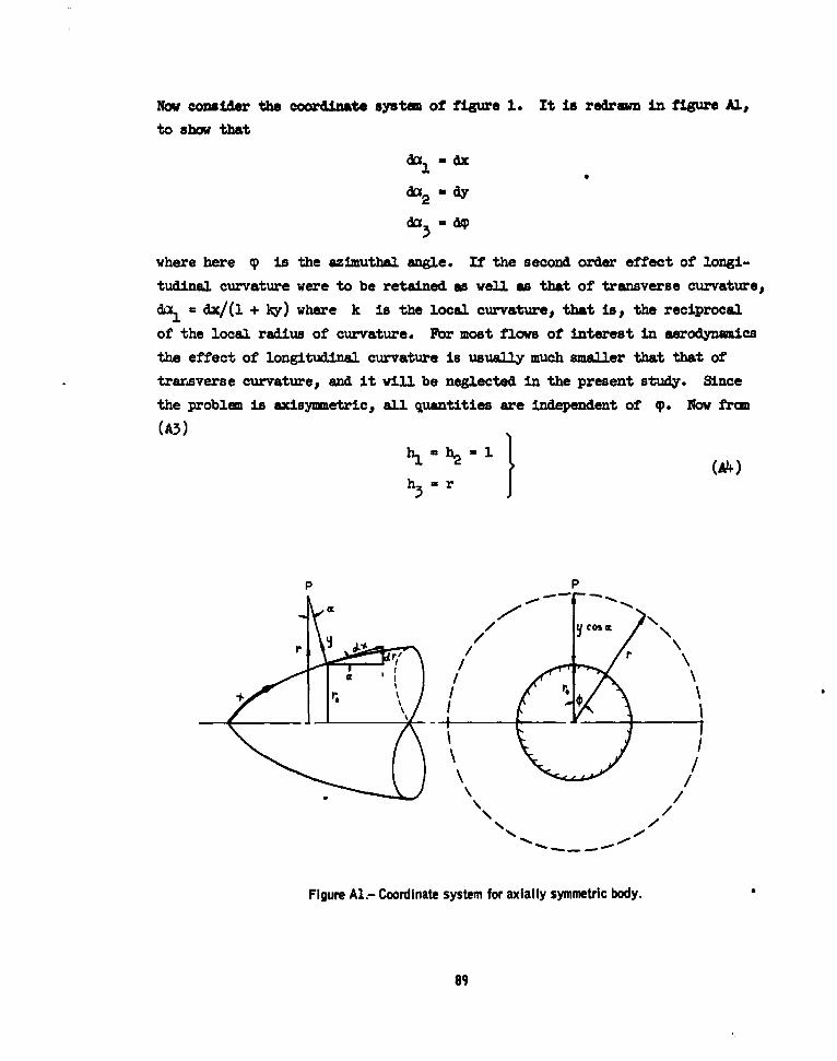
Now consider the coordinate system of figure 1. It is redrawn in figure All
to show that
d2- dx
where here (p is the azimuthal angle. If the second order effect of longi-
tudinal curvature were to be retained as well as that of transverse curvature,
da1 - dx/(l + ky) where k is the local curvature, that is, the reciprocal
of the local radius of curvature. For most flows of interest in aerodynamics
the effect of longitudinal curvature is usually much smaller that that of
trarsverse curvature, and it will be neglected in the present study. Since
the problem is sxisymmetric, all quantities are independent of q). Now from
(A3)
h1, 2 ( A}
P P
I -
I I
\/
Figure AL- Coordinate system for axially symmetric body.
89
From vector analysis and the relation
V-Tu+ v (As)
the continuity equation can be written
d+ v (pV + 1 p (A6)
Momentum Nauation
The Navier-Stokes equation of motion in vector notation is (from page 50
of Howarth, Reference 5):
(V +gradV).P-ra p+ ( + grd (V ra )
-V±+ grad gX curlV-agrad p
- curl curl V V (A7)
In order to apply the boundary-layer assumptions, consider the x and y
components of (A7) separately. The x-vise or 1 component in the orthogonal
coordinate system is:
6+ + u V-TY1
+16u,
where Y is 1 body force.
90
Now make the usual order of magnitude analysis of (AS). Let ue, pe end
x be of order unityp that isj, ue pep x - 0(1). Then since
Rx --a-, 11 -o (I
Also since, o )
Similarly, the magnitude of the other caponents of (AB) may be found. They
are siumarized in the table below.
OMDR QUAYT=
22u°(8"2)
o(-1)
au a u a% vo(l) r., u. x. ps -, 0, UT-- S,
v arv a2 v00) V J R , ME
o(e2 ) v -PI/,
If only terms of order (8) or larger-,that is, terms of order (8), (1), (5"),
(5-2) -are retained, then eq.(AB) reduces to the following equation,
S + u + v Y +a2(A9)
The y or _j component of equation (A7) is
91
+ N+ +(W -.1r)
" r +a , 2 aa;u Y F v '6
If terms of order unity are retained, (AIO) reduces to
pdy
For the flow under consideration there are no body forces and the flow issteady. The m~nentum equations (A9) and (All) then become
PLu +Vy] =--+r~ (u+
. 6- (Al3)
The latter says that the total change of pressure through the boundary layernormal to the surface is of order 52 . Therefore it wifl be neglected, and
the partial derivative of pressure with respect to x, p/ x, is replaced
by the total derivative, dp/dx, in eq. (A12).
Ebergy Equation
The basic form of the energy equation for an orthogonal coordinate systanis given by Howrth, page 55, Reference 5. In his notation
+216r + v + r+1TrXu
+h a 0 F6(g(v) - (4AP)
where h = enthalpy =fcp d
F o dhl iption function = rate of work done by viscous forces
92
and by definition
D ( + V • (A15)
k6)-dv(kc grad T) (A16)
The dissipation term in vector coordinates is given by
div grad V 2 2 div Xcl V) - 2 V.d(div v) + (r V) 2 - 2 (dv V)2
(A17)An order of magnitude analysis as was made above for the manentum equation
gives, if terms of only the highest order are retained, •
=h ahu ah 6Tk ) (A.8)
The last term can be written in terms of enthalpy by the relation
k T =k__ ah k ah . g ah A9Ty -p T- acp P sy
where Pr is the Prandtl number. Substitution of (A19) in (A18) gives
rah bh ah u &k + ', (au~~~ FY)~+J~ +~ +F 1 aj[ (A20)
Now if steady flow is assumed and if the momentun equation (A12) is used to
replace the term u t p (A20) may be written
[ (21h)
Now introduce total enthalpy H
12
93
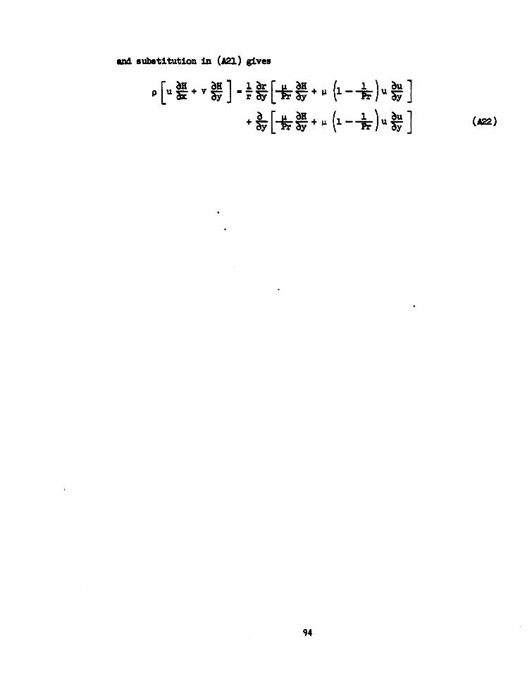
aMt substitution in (A21) gives
U + v u =.1 + i u au
94
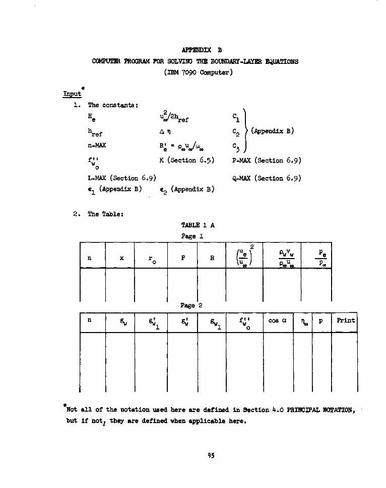
APPMMIX BCOMPtI PROGRAM FOR SOLVING THE BOUNDARY-L EQUATIONS
(IBM 7090 Computer)
Input
1. The constants:
He u:/2hr C1
href a q C2 (Appendix B)
n-MAX ' = pU/- C 3
f" K (Section 6.5) P-MAX (section 6.9)w0L-MAX (Section 6.9) Q-MAX (Section 6.9)61 (Appendix B) e2 (Appendix B)
2. The Table:
TABLE 1 A
Page 12
n x P R (-Le Pwvw
Page 2
n 9w ; 9; fZ' cos a i p Print1. 1 0 _
Not all of the notation used here are defined in Section 4.0 PRINCIPAL NOTATION,
but if not1 they are defined when applicable here.
95
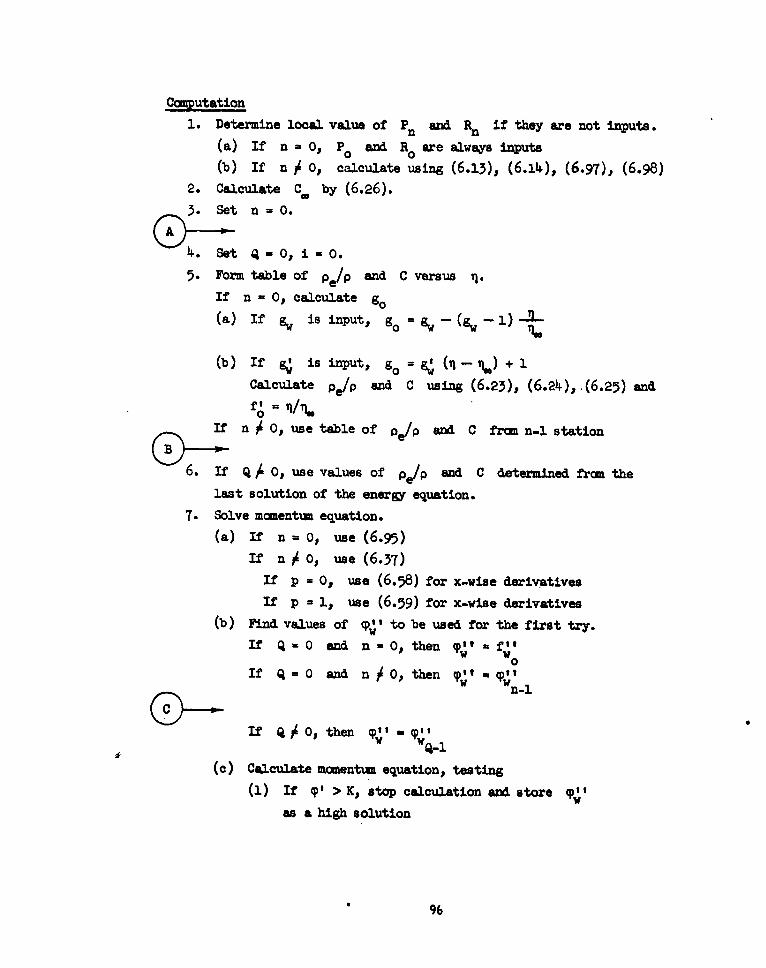
Ccaputation1. Determine local value of Pn and Rn if they are not inputs.
(a) If n= 0 P0 and Re are always inputs(b) If n j 0, calculate using (6.13), (6.14), (6.97), (6.98)
2. Calculate C by (6.26).
3. Set n=O.0-4. Set Q=O, i=O.
5. Form table of pe/p and C versus T1.
If n - O calculate go
(a) If gw is input, go = gw-(gw-
(b) If g is input, go = g (n-% ) + iCalculate pep and C using (6.23), (6.24), (6.25) and
fo = n/l%If n 0, use table of pe/p and C fro n-l station
6.If 0, use values of p/p and C determined from the
last solution of the energy equation.
7. Solve momentum equation.
(a) If n =O, use (6.95)If n . use (6.37)
If p = 0, use (6.58) for x-wise derivatives
If p = 1, use (6.59) for x-wise derivatives(b) Find values of (p," to be used for the first try.
If Q -0 and n = 0, then , = fitIW
0If Q=O and njO, then (ptt-"w t"
If Q j 0, then (pwtI 9"l -
(c) Calculate momentum equation, testing(i) If (' > K, stop calculation and store pI
as a high solution
96
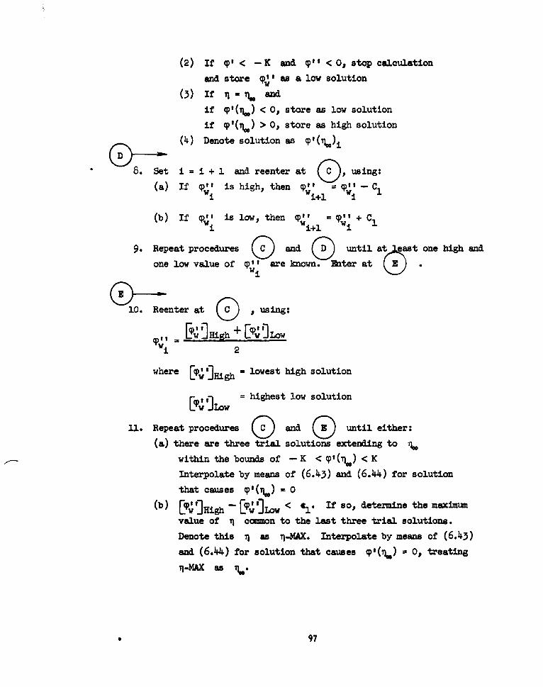
(2) If (' < -IC and C" <0, stop calculation
and store Cp' as a low solution
(3) If r andif '(%) < 0, store as low solution
if ( ) > 0, store as high solution
D() Denote solution as ( )i
8. Set i = i + 1 and reenter at C , using:
(a) If wi is high, then cWi' = c"w' -C I
i Wi+l = iP';-C
(b) If cpw" is low, then ='w + C1
9. Repeat procedures ( and D until a ast one high andone low value of pwi are known. Rater at
10. Reenter at , using:
*±wl 2
where [ w"]High = lowest high solution
w= highest low solution
311. Repeat procedures G) and (i' until either:(a) there are three trial solutions extending to r6
within the bounds of - K < (P(Ti) < KInterpolate by means of (6.43) and (6.44) for solution
that causes 9'(%) = 0(b) [pt']High -- ']Low < a,. If so, determine the maximum
value of Y common to the last three trial solutions.
Denote this il as q-MAX. Interpolate by means of (6.43)and (6.44) for solution that causes 0'(.) - 0, treating
TI-MAX as
• 97
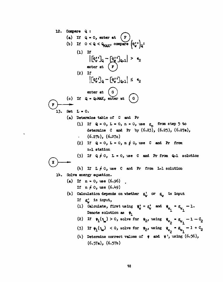
12. Compare Q :
(a) If Q - O, enter at F )(b) If O<Q< . compare ((P') I
(1) if
enter at
(2) If
enter at 0
(c) If Q= Q-MAX, enter at
13. Set L=O.(a) Determine table of C and Pr
(1) If Q = Op L = 0, n = Op use g0 from step 5 to
determine C and Pr by (6.23), (6.25), (6.27a),
(6.27b), (6.27c)
(2) If Q = O, L =0, n 0, use C and Pr from
n-i station
(3) If Q O, L 0, use C and Pr fran Q-1 solution
(4) If L 0 0, use C and Pr from L-1 solution
14. Solve energy equation.
(a) If n O, use (6.96)
If n 0., use (6.49)(b) Calculation depends on whether g. or gw is input
If g is input,
(1) Calculate, first using *1 = and - 1.
Denote solution as * 1
(2) If *(il) >0, solve for *20 using ww2 = S1-1-C 2
(3) If *1(n=) < O, solve for *2p using *, - g1 - + C2w2 1
(4) Determine correct values of * and *' using (6.56),
(6.57a), (6.-57)
98
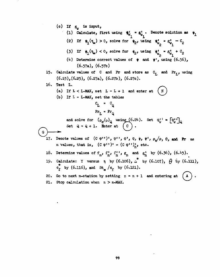
(c) If is input,
(1) Calculate, first using 1 .Denote solution as
(2) If *1(%) > 0, solve for 'p2' using = 91 + C2
'2 1(,) Iftl <0o, solve for 'p2' usn tw = gl' *C2
(4) Determine correct values of * and *' , using (6.56),
(6 .57a), (6.57b)15. Calculate values of C and Pr and store as CL and PrL, using
(6.23),(6.25), ( 6 .27a), (6.2Tb), (6.27c).
16. Test L.
(a) If L < L-MAX, set L = L + 1 and enter at (H)(b) If L = L-MAX, set the tables
CL = CQ
Pr L = Prq
and solve for (p /P) usin 6.24). Set c -
Set Q=Q + . Rter at
17. Denote values of (C (p")', cp, 'I', r, *1 ', pe/p , C, and Pr as
n values, that is, (C qI")' = (C (pI")' etc.
38. Determine values of fn f': f", g and q by (6.36), (6.45).n n n n
19. Calculate: Y versus I by (6.106), a by (6.107), 0 by (6.1U/),Cf by (6.116), and St /cf by (6.121).
20. Go to next n-station by setting n = n + 1 and entering at 021. Stop calculation when n > n-MAX.
99
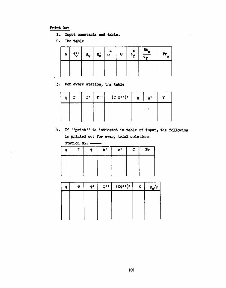
Print Out
1. Input constants and table.
2. The table
n W1 I g g * f C P r
3. For every station, the table
T f ft fit (C CP)I g gI Y
.. If "print" is indicated in table of input, the following
is printed out for every trial solution:
Station No.
1 Tr r t' C Pr
(P cps I (cq" I) I C Pe/P
100
1. Smith$ A. M. 0. and Clutter, D. W.:-Solution of the IncompressibleLinni Boundary Layer Equations. Douglas Aircraft Co. Report No.
zs 4o446, Juy 29, 1961.
2. Smith, A. M. 0. and Clutter, D. W.:-Solution of the IncompressibleLainar Boundary Layer Equation. Douglas Aircraft Co. Engineering
Paper No. 1525, January 1, 1962.
3. mith, A. M. 0. and Clutter, D. W.:-Solution of Prandtl'a Boundary-
Layer Equations. Douglas Aircraft Co. Engineering Paper No. 1530,
February 2, 1962.4. Van Dyke, M. :-Second-Order Compressible Boundary-Layer Theory with
Application to Blunt Bodies in Hypersonic Flow. Stanford University
Department of Aeronautical Engineering Report suDaR No. 112, July 1961.5. Howarth, L. :-Modern Developments in Fluid Dynamics. Vol. 1, Oxford 1953.6. Flflgge-Lotz, I. and Blottner, F.G.:-Computation of the Compressible
Laminar Boundary-Layer Flow Including Displacement-Thickness Interaction
Using Finite-Difference Methods. Stanford University Division of
Engineering Mechanics Technical Report No. 131, January 1962.
7. Cohen, N. B. :-Correlation Formula and Tables of Density and Some
Transport Properties of Equilibrium Dissociating Air for Use in
Solution of the Boundary-Layer Equations. NASA TN D-194, February 1960.
8. Hartree, D. R. and Womersley, J. R.:- A Method for the Numerical or
Mechanical Solution of Certain Types of Partial Differential Equations.
Proc. Royal Soc. Series A, Vol. 161, No. 906, P.353, August 1937.
9. Hartree, D. R. :-A Solution of the Laminar Boundary-Layer Equation for
Retarded Flow. British R and M No. 2426, 1949.
10. Hartree, D. R. :-The Solution of the Equations of the Laminar Boundary
Layer for Schubauer's Observed Pressure Distribution for an Elliptic
Cylinder. British R and M No. 2427, 1949.
11. Collatz, L. :-The Numerical Treatment of Differential Equations. Third
mltion. Springpr-Verlag 1960.12. Hildebrand, F. B. :-Introduction to Numerical Analysis. McGraw Hill, 1956.
13. Hayes, Wallace D., and Probstein, Ronald F. :-Hypersonic Flow Theory.
Academic Press, 1959.
101
14. Cohen, C. B., and Resbotko, E.:-Similar Solutions for the Compressible
Laminar Boundary Layer with Heat Transfer and Pressure Gradient. NACA
Report 1293, 1956.
15. Chapman, D. R. and Rubesin, M. W.:-Temperature and Velocity Profiles in
the Compressible Laminar Boundary Layer with Arbitrary Distribution of
Surface Temperature. J. Aero. Sci. Vol. .6 5147 (1949).
16. Low, G. M. :-The Compressible Laminar Boundary Layer with Heat Transfer
and Small Pressure Gradient. NACA TN 3028, October 1953.
17. Beckwith, I.E., and Cohen, N. B. :-Application of Similar Solutions to
Calculation of Laminar Heat Transfer on Bodies with Yaw and Large
Pressure Gradient in High-Speed Flow. NASA TN D-625o January 1961.
18. Cohen, C. B. and Reshotko, E.:-The Copressible Laminar Boundary Layer
with Heat Transfer and Arbitrary Pressure Gradient. NACA Report 1294.,
1956.
19. Probstein, R. F. and Elliott, D. :-The Transverse Curvature Effect in
Compressible Axially Symmetric Laminar Boundary-Layer Flow. J. of
Aeronautical Sciences, Vol. 23, No. 3, March 1956, pp. 208-224, 236.
102
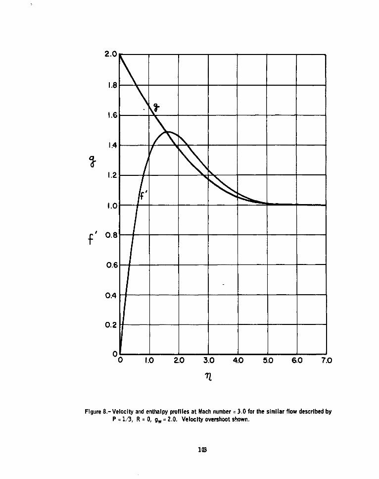
2.0
1.2
1.6.
0.4
0.2
1.01
0.43
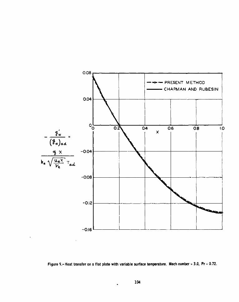
0.08
-- -PRESENT METHOD
-CHAPMAN AND RUBESIN
0.04
0 0.G04 0.6 0.8 1.0
i x -0.04
-0.08
-0.12
-0.16
Figure 9.- Heat transfer on a flat plate with variable surface temperature. Mach number 3.0, Pr 0.72.
104
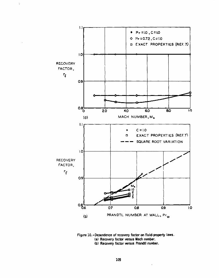
I.'
* Pr=j.0 ,C=I.O
0 Pr =0.72, C= 1.0
0 EXACT PROPERTIES (REF.7)
1.0 -
RECOVERY
FACTOR,
0.9
0.80 2.0 4.0 6.0 80
(a) MACH NUMBER, Me
1.10 C=I1.0
O EXACT PROPERTIES (REF.7)
- -'- SQUARE ROOT VARIATION
1.0 .0
RECOVERY
FACTOR, . e
rf - ____
0.9 -
*Io
3
.6 0.7 0.8 0.9 1.0
(b) PRANDTL NUMBER AT WALL, Pr w
Figure 10.-Dependence of recovery factor on fluid-property laws.(a) Recovery factor versus Mach number.(b) Recovery factor versus Prandtl number,
105
1.2
M. R.
O 3.94 67000 3.90 3800
EXPERIMENTAL 0 4.15 2000
0 5.50 22001.0 = UGDo D
PRESENT METHOD
Jw 0.8
Y[LO1w]L c W STAG
0.6
0.4
0
0.2 O
5.500 ~0
00 30.0 60.0 90.0 120.0
0 (ANGULAR DISTANCE)
Figure 11.-Comparison of heat transfer calculated by the present method with thatmeasured In the wind tunnel for a circular cylinder.
106
6.0a 2.82SIx 10 FT/SEC.
He =27.248XIO FTYSEC.2
5.0 1W 0.17825 /
4.0
r)
U~e
a. 3.0
MeMe
2. 0 '
00 1.0 2.0 3.0 4.0 5.0 6.0
AXIAL DISTANCE,X
Figure 12.-Variation of surface distance x, body radius r,, u.*/a*, and M,* with axial distance forthe rocket nozzle problem. H. = 27.246 X106 ft2/sec 2; g,,= 0.17625; Pr = 0.78.
107
1.2
JC X13 C7
00
1.6
1.2 NOZ ZLESt THROAT
0
1.6 07 . .
EXAC THROATIE
010203.0 4.0 5.0 6.0x
(b)
Figure 13.- Results of calculation for the rocket nozzle.(a) Skin friction. (b) Ratio of Stanton number to skin friction.
108
5.0
Ue4.0
X 0P3.0
2.0
at
1.0
SPH:ERE ICONE
0102.0 3.0 4.0 5.0
AXIAL DISTANCE, X
Figure 14.-VariatIon of local velocity, body radius and surface distance with axial distancefor a spherically blunted cone. M. = 3.0 and 9.0.
109
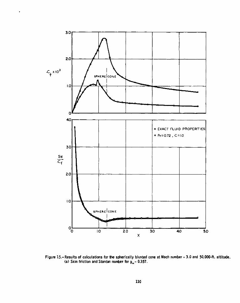
3.0
2.0
~CX10 3f SPHEREICONE
40
oEXACT FLUID PROPERTIES
*Pr =O.72 , C = .0
3.0 -____
St,Cf
2.0 ____
1 .C
0102.0 3.0 4.0 5.0
Figure 15.- Results of calculations for the spherically blunted cone at Mach number =3.0 and 50,000-ft. altitude.(a) Skin friction and Stanton number for g,,= 0.357.
110
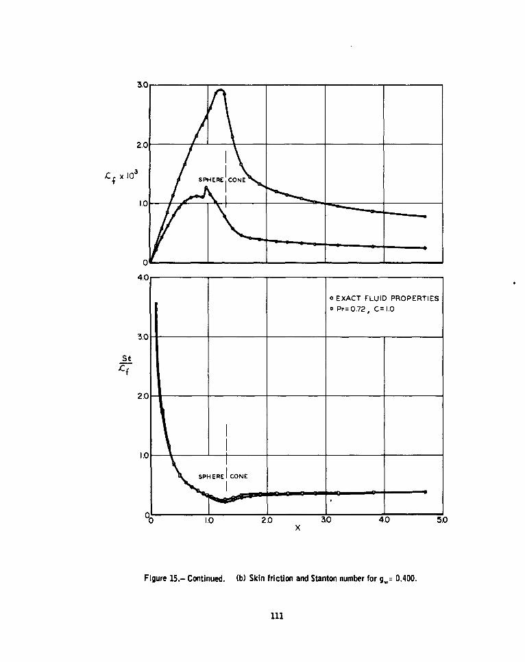
5.0
2.0
)c 10 SPHERE CONE ,
4.0
0 EXACT FLUID PROPERTIES
3.0 a Pr= 0.72, C= 1.0
Ic f
2.0
SPHERE' CONE
0 1.0 2.0 30 4.0 5.0X
Figure 15.- Continued. (b) Skin friction and Stanton number for g,= 0.400.
ill
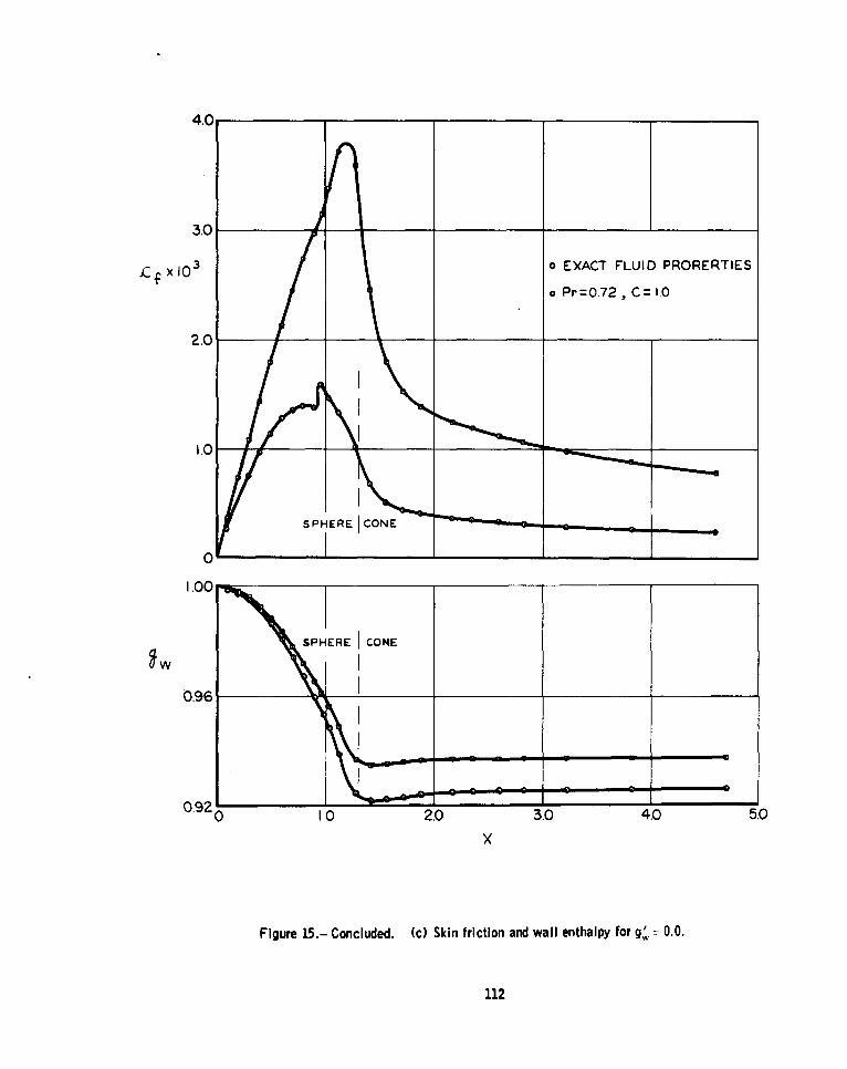
4.0
3.0-
xc X1 3o EXACT FLUID PRORERTIESoPrO.72, C= 1.0
2.0-
l.0
1.00SPH-ERE ICOME
0.96-
0*2 1.0 2.0 3.0 4.0 5.0
x
Figure 15.-Concluded. (c) Skin friction and wall enthalpy for gw' = 0,0.
112
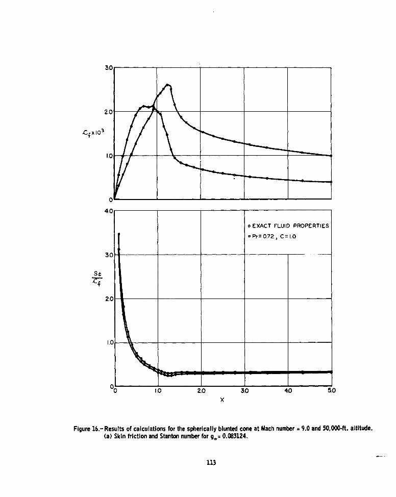
3.0
2.0
,Cf x I0
1.0
0
4.0
o EXACT FLUID PROPERTIES
o Pr= 0.72, C=1.0
3.0
StZ4
2.0
I.0-
1.0 2.0 3.0 4.0 50
x
Figure 16.-Results of calculations for the spherically blunted cone at Mach number = 9.0 and 50,000-ft. altitude.(a) Skin friction and Stanton number for g,= 0.083124.
113
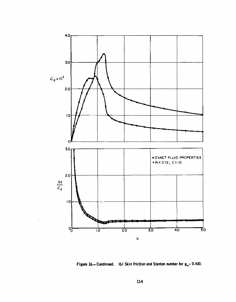
4.0
3.0
2.0
1.0
3.0 -_ _ _ _ _ _ _ _ _ _ _ _ _ _ _
0 ExACT FLUID PROPERTIESaPr= 0.72, C= 1.0
2.0 -____ __________
St
IC
10
0OL 1.0 2.0 3.0 4.0 5.0
x
Figure 16.- ContInued. (b) Skin friction and Stanton number for g,,= 0.400.
114
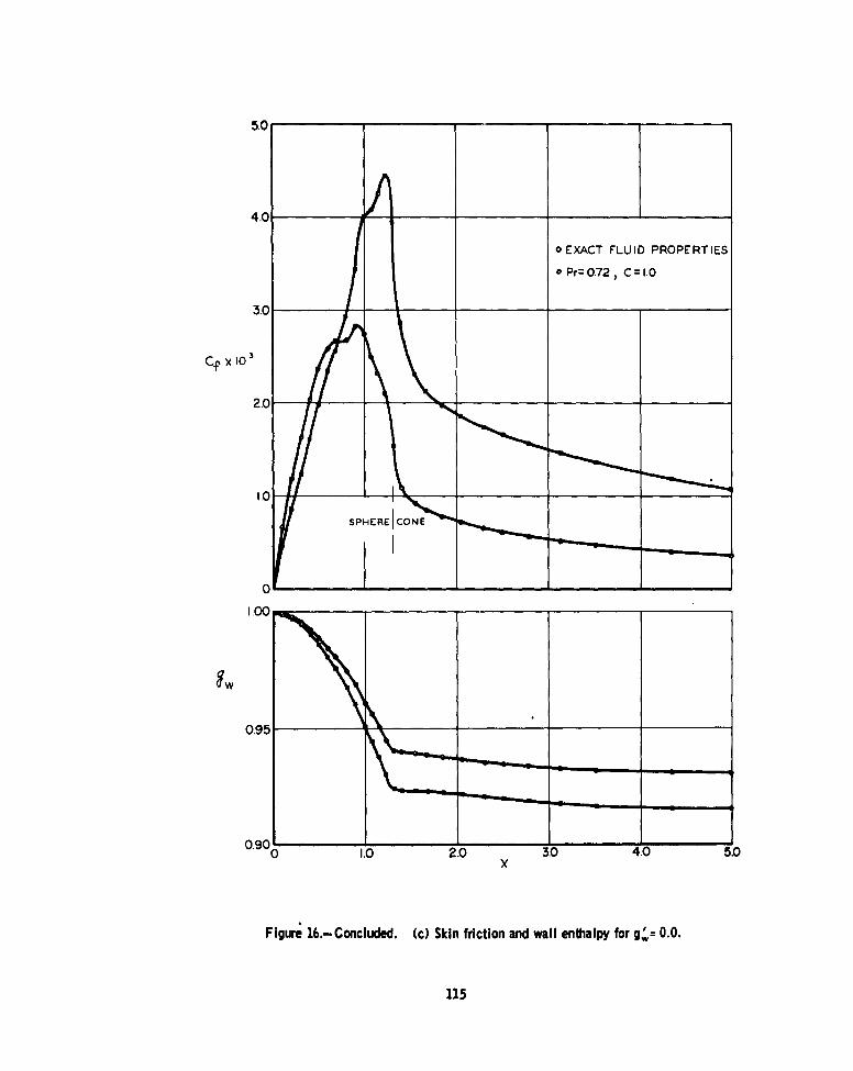
5.0
4.0
* EXACT FLUID PROPERTIES
* Pr=072, C 1. 0
3.
CfX10,
2.0
SPHERE CONE
1.00
0.95-
0.900 .2.30405
Figure 16.-Concluded. (c) Skin friction and wail enthalpy for g'= 0.0.
115
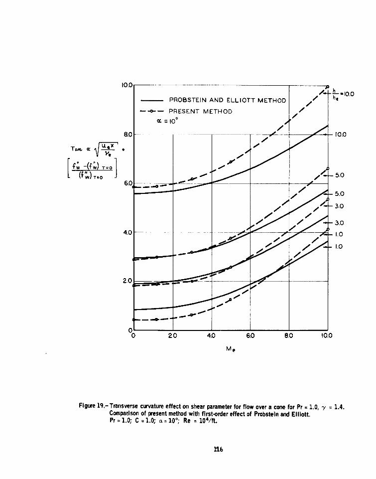
PROBSTEIN AND ELLIOTT METHOD he 10.
-o-PRESENT METHOD7
= 1000
_000 3.0
E. - 1.0-(~~=
0 2.0 4.0 6.0 8.0 10.0
M e
Figure 19.- Transverse curvature effect on shear parameter for flow over a cone for Pr =1.0, y = 1.4.Comparison of present method with first-order effect of Probstein and Elliott.Pr = 1.0; C = 1.0; a = 100; Re = 104/ft.
116
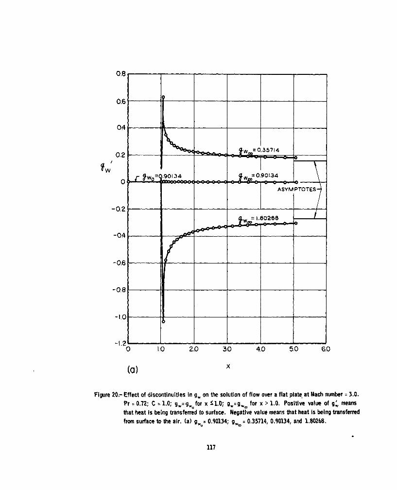
0.8
0.6
04
0.20.51W/I
9 .01340.9014
-0.2 06
-04
-0.6
-0.8
0 1.0 2.0 3.0 4.0 5.0 6,0
W~) X
Figure 20:- Effect of discontinuities In g, on the solution of flow over a flat plate. at Mach number =3.0.
Pr =0.72; C =1.0; g,,= gwofor x S 1.0; g = g for x > 1.0. Positive value of g' meansthat heat Is being transferred to surface. Negative value means that heat is being transferredfrom surface to the air. (a) gwo 0.90134; gWW = 0.35714, 0.90134, and 1.80268.
117
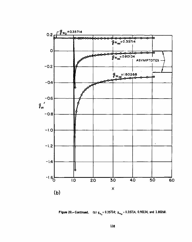
0.2 r IWO.357I4 -
0
-0=.21
-0.6-
-0.8
-1.0
-14
O10203.0 4.0 5.0 6.0
(b)
Figure 20.- Continued. (b) gw= 0.35714; g ,, 0.35714, 0.90134, and 1.80268.
118
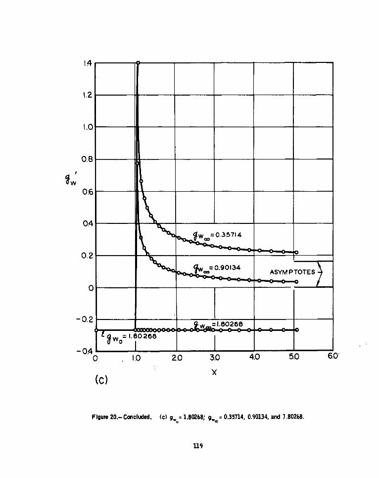
14____
0.8
fw0.6
04 = . 5 1
0.2
0
-0.2 1:. 80288
-0411 -0 .1.0 2.0 3.0 4.0 5.0 6.0*
(C)Y
F igure 20.- Concluded. (c) gw,= 1.80268; gwc = 0.35714, 0.90134, and 1.80268.
119
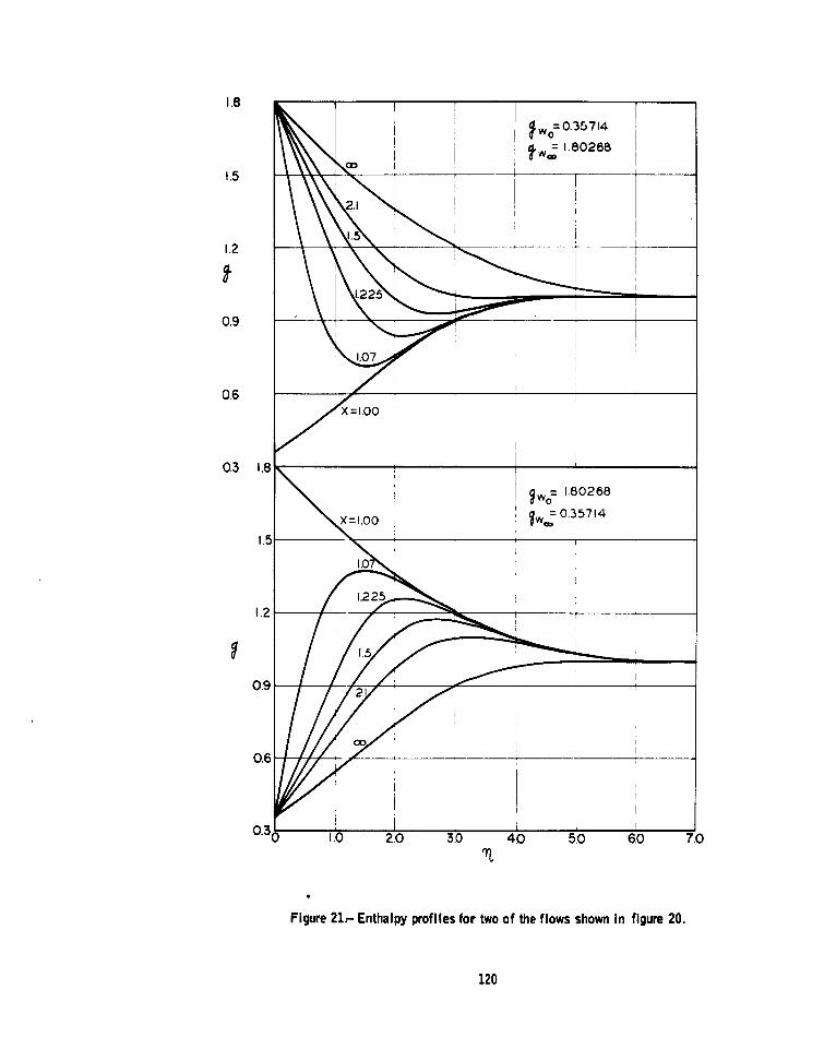
WC .802r8
1.5 _____C
2X.
01.5
1.2
0.3o ~~1.20.0 50 6 .
1.070
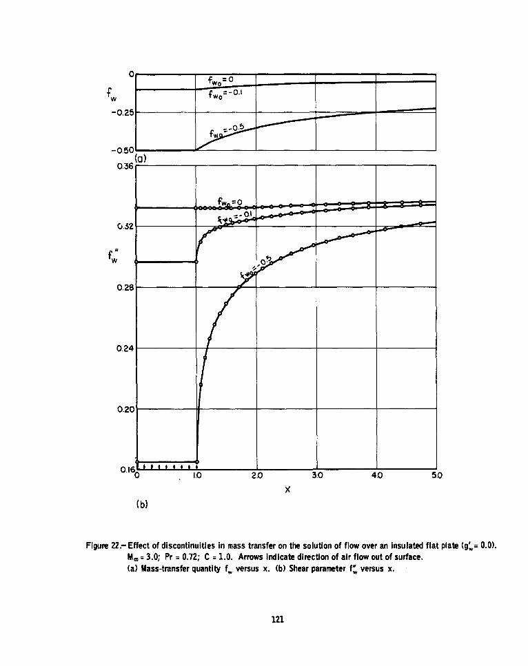
0 0 f =0
-0.25 .
-0.50 (a)0.36
0.2.1
0.24
0.20
0 10 2.0 3.0 4.0 5.0
x(b)
Figure 22-Effect of discontinuities in mass transfer on the solution of flow over an insulated flat plate (g',= 0.0).M. = 3.0; Pr = 0.72; C = 1.0. Arrows indicate direction of air flow out of surface.(a) Mass-transfer quantity f,, versus x. (b) Shear parameter f'w, versus x.
121
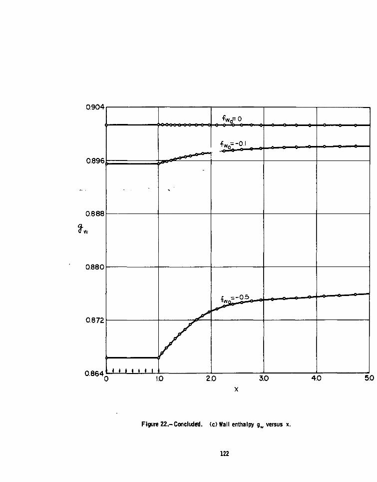
0.904___. ... .. . ...fvv o_ _ _ _
f.-= -0.1
0.896
0.888-
0.880
0.872 1
0.8640 i a a a _ _ _ _ _ _ _10 2.0 3.0 4.0 5.0
x
Figure 22.- Concluded. (c) Wall enthalpy g,, versus x.
122
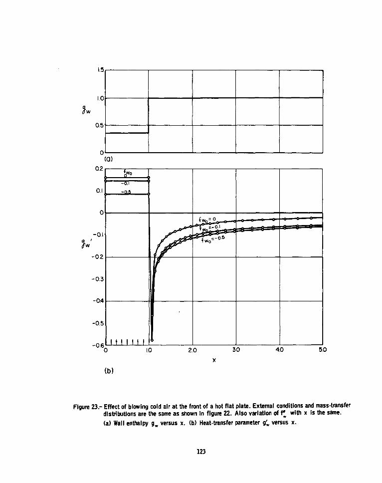
1.0IO
0.5
0(M)
02 w -o
-0.1
0.1
-0.1
-0.3
-04
-0.5
0 1,0 2.0 3.0 40 5.0
x
(b)
Figure 23.- Effect of blowing cold air at the front of a hot flat plate. External conditions and mass-transferdistributions are the same as shown in figure 22. Also variation of fl, with x is the same.
(a) Wall enthalpy g. versus x. (b) Heat-transfer parameter g' versus x.
123
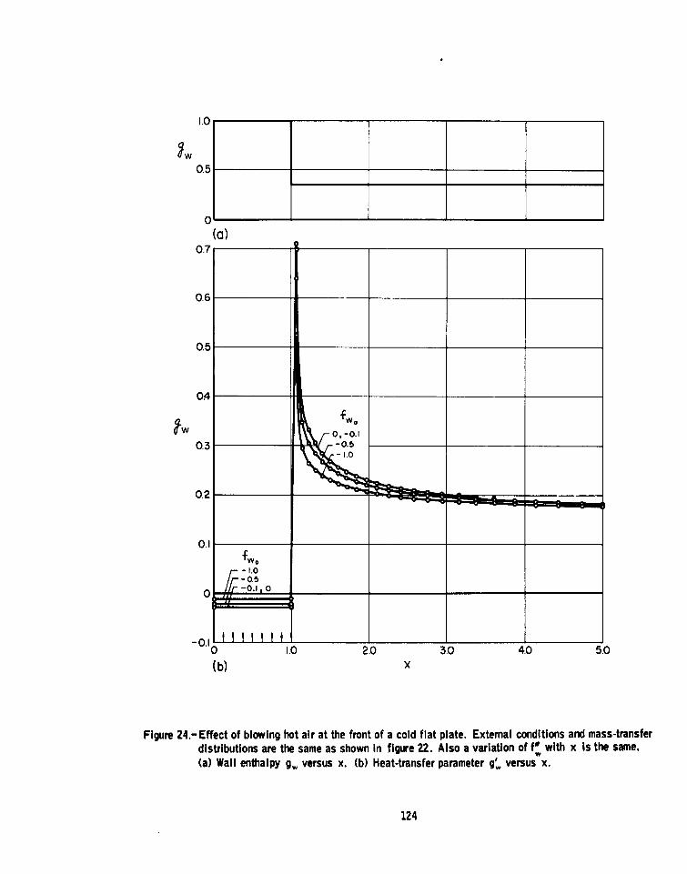
1.0
0.5
0
(a)0.7
0.6
04
0.3 -.
0.2
0.1
o wo
-0.11 1 f t i
-1.0-0.5
0.0 2.o 3.0 4.0 5.0(b) X
Figure 24.- Effect of blowing hot air at the front of a cold flat plate. External conditions and mass-transferdistributions are the same as shown In figure 22. Also a variation of f" with x is the same.(a) Wall enthalpy g, versus x. (b) Heat-transfer parameter g' versus x.
124
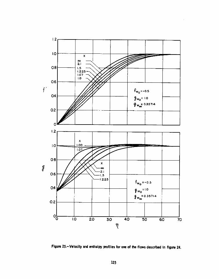
1.2
1.0
0.80
060
04-f=0.
Tw. 0.35714
.2
-
0
0.2
0.0 1.00 20 30 40 . . .
212
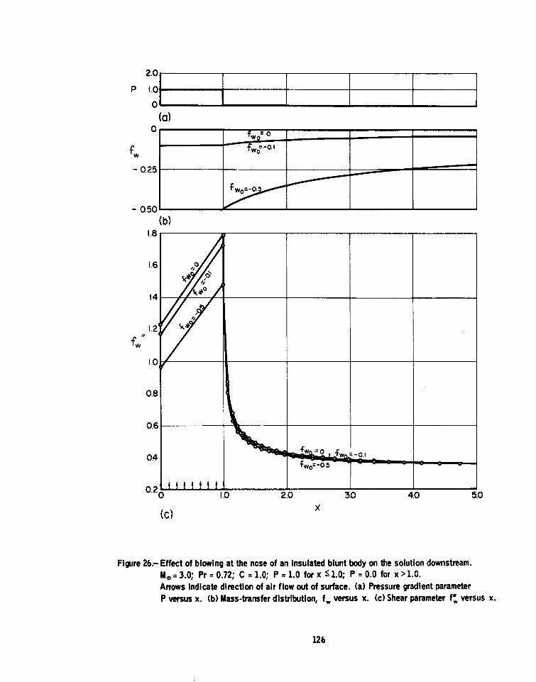
P 1.0 10(a)
0fw=
- 0.25
- 0.50(b)
1.8
1.6
4
1.2
1.0f
0.8
0.6
04 rw=0 ~
0.2t _____0 1O0 2.0 3.0 40 5.0
(c) x
Figure 26- Effect of blowing at the nose of an Insulated blunt body on the solution downstream.M. = 3.0; Pr = 0.72; C = 1.0; P = 1.0 for x < 1.0; P = 0.0 for x > 1.0.Arrows Indicate direction of air flow out of surface. (a) Pressure gradient parameterP versus x. (b) Mass-transfer distribution, f,, versus x. (c) Shear parameter f, versus x.
126
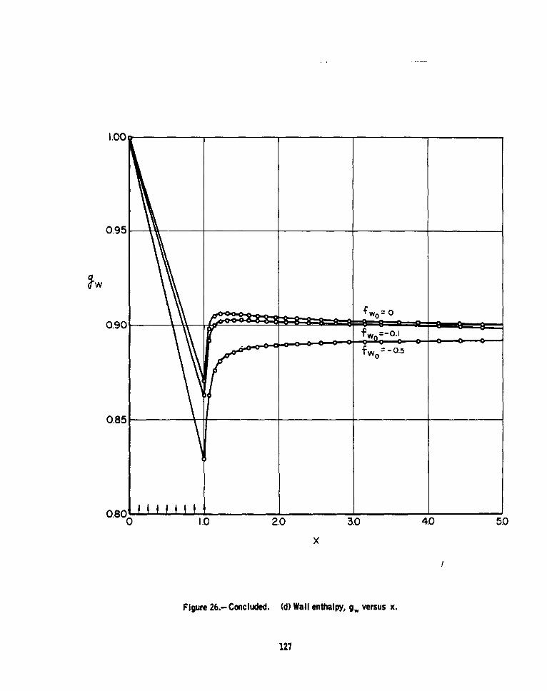
1.00
0.95
;wo= 0,0.90 1
0.85
00 2.0 3.0 4.0 5.0
x
Figure 26.- Concluded. (d) Wall enthalpy, g, versus x.
127
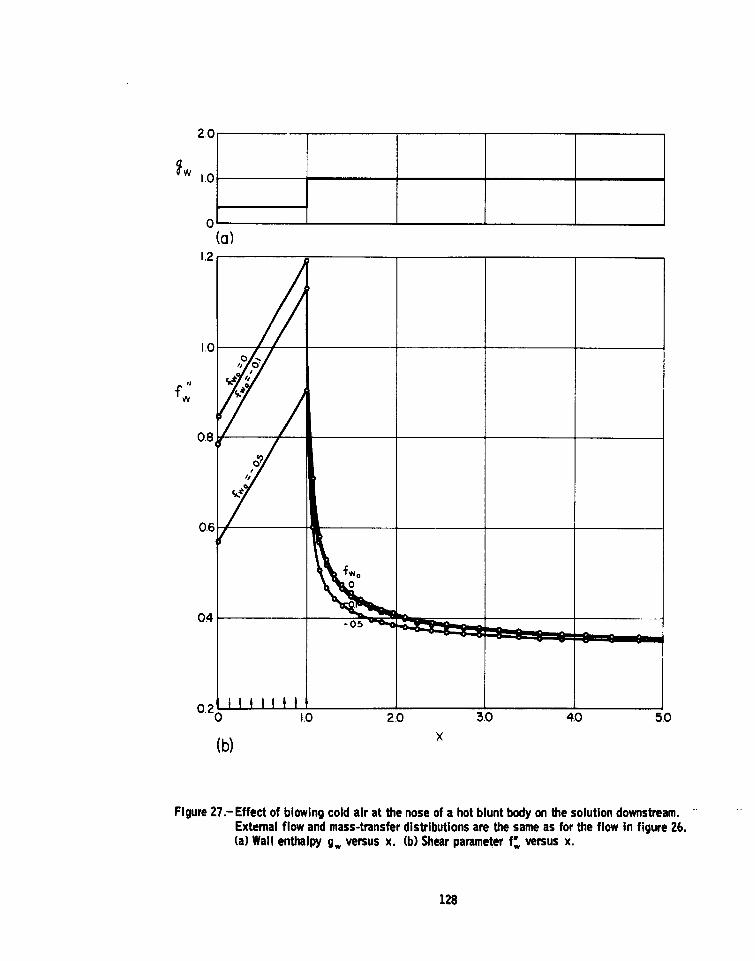
2.0
1.0
0(a)
1.2
0%
0.8
0.6/
040
0.201 I. 0 2.0 3.0 4.0 5.0
(b) x
Figure 27.- Effect of blowing cold air at the nose of a hot blunt body on the solution downstream.External flow and mass-transfer distributions are the same as for the flow in figure 26.(a) Wall enthalpy g, versus x. (b) Shear parameter f, versus x.
128
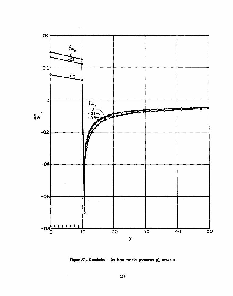
0.4
fw 0
-01
0.2
-0.5
00
-0.2
-04
-0.6
0. . 3.0 4.0 5.0
x
Figure 27.- Concluded. - (c) Heat-transfer parameter g' , versus x.
129
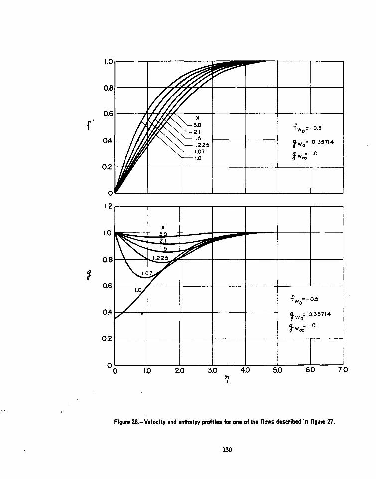
1 .0
06
5.0 fw0 =0.5
04- . 0.35714
1.07 w = 1.0
0.2 -r& .
0
1.2
1.00
0.6 __\-_7
04 fv o . 7I
0.2__
00 1.0 2.0 3.0 4.0 5.0 6.0 7.
Figure 28.-Velocity and enthalpy profiles for one of the flows described In figure 27.
130
DISTRIBUTION LIST FOR DOGLAS AIRCRAFT CO. REPORT NO.
LB 31088, CONTRACT NO. NOv 60-0533c
NAVY AIR FORCE
Chief, Bureau of Naval Weapons CommanderDepartment of the Navy Office of Aerospace ResearchWashington 25, D. C. Washington 25, D. C.Attn: Code RRRE-4
Code RAAD-3 Directorate of AeromechanicsCode DLI-31 USAF Aeronautical Systems Division
Wright-Patterson Air Force Base, OhioCommanding Officer and DirectorDavid Taylor Model Basin Arnold Engineering Development CenterCarderock, Maryland P.O. Box 162Attn: Aerodynamics Laboratory Tullahoma, Tennessee
CommanderNaval Missile Center ARMYPoint Mugu, California
Office of Ordnance ResearchCommander Department of the ArmyNaval Ordnance Test Station Duke StationInyokern, China Lake, California Durham, North CarolinaAttn: Technical Library
Ballistic Research LaboratoryCommander Aberdeen Proving GroundNaval Ordnance Test Station Aberdeen, MarylandPasadena AnnexPasadena, California OTHER GOVERNMENT AGENCIESAttn: Technical Library
CommanderCommander Armed Services Technical Information AgencyNaval Ordnance Laboratory Arlington Hall StationWhite Oak, Silver Spring, Maryland Arlington 12, VirginiaAttn: Code HL
Code DA National Aeronautics and SpaceAdministration
Commander 1512 H Street N.W.Naval Weapons Laboratory Washington 25, D. C.Dahlgren, VirginiaAttn: Technical Library Director
National Bureau of StandardsChief of Naval Research Washington 25, D. CDepartment of the Navy Attn: Fluid Mechanics SectionWashington 25, D. C.Attn: Code 438
Code 461
IDUCATICUAL INSUICTZ INDUSTRIAL CSMIIZATIMS
Guggenheim Aeronautical Laboratory Lima-Temco-Voust-CorporationCalifornia Institute of Technology P.O. Box 1508Pasadena 4, California Dallas 22, TexasAttn: Dr. Clark B. Millikan
General ynua es/ConvairApplied Physics Laboratory P.O. Box 1950Johns Hopkins University San Diego 12, CnliforniaP.O. Box 244 - Ht. 1 Attn: Mr. C. W. FrickLaurel, MarylandAttn: Technical Reports Office Grumman Aircraft Engineering Corporation
Bethpage, Long Island, New YorkDepartment of Aeronautics Attn: Fluid Mechanics SectionJohns Hopkins UniversityBaltimore 18, Maryland Lockheed Aircraft CorporationAttn: Dr. F. H. Clauser Burbank, California
Attn: Mr. L. A. RodertInstitute for Fluid Mechanicsand Applied Mathemtics McDonnell Aircraft CorporationUniversity of Maryland St. Louis, MissouriCollege Park, Maryland Attn: Mr. G. S. GraffAttn: Professor J. M Burgers
Norair DivisionMassachusetts Institute of Technology Northrop CorporationCambridge 39, Massachusetts 1001 East BroadwayAttn: Aerophysics Laboratory Hawthorne, California
Attn: Dr. W. PfenningerDefense Research LaboratoryUniversity of Texas North American Aviation, Inc.P.O. Box 8029 Aerophysics DepartmentAustin, Texas 12214 Lakewood BoulevardAttn: Professor M. J. Thompson Downey, California
Attn: Dr. E. R. Van Driest
North American Aviation, Inc.4300 East 5th Avenue
Columbus, OhioAttn: Mr. R. M. Crone
Cornell Aeronautical Laboratory4455 Genesee St.Buffalo 21, New York
. II11i I I Ii
'
a all
IiIlag 1 1 I
OZ Q
.H a , ! a
I tti la!11bj i iiJ!l t