A Variational Method for the Analysis of Three …twister.caps.ou.edu/DualDoppler98/GaoDual1999.pdf2128 MONTHLY WEATHER REVIEW VOLUME 127 q 1999 American Meteorological Society A Variational

2128 VOLUME 127M O N T H L Y W E A T H E R R E V I E W

q 1999 American Meteorological Society

A Variational Method for the Analysis of Three-Dimensional Wind Fields from TwoDoppler Radars

JIDONG GAO AND MING XUE

Center for Analysis and Prediction of Storms, University of Oklahoma, Norman, Oklahoma

ALAN SHAPIRO AND KELVIN K. DROEGEMEIER

Center for Analysis and Prediction of Storms and School of Meteorology, University of Oklahoma, Norman, Oklahoma

(Manuscript received 29 May 1998, in final form 28 August 1998)

ABSTRACT

This paper proposes a new method of dual-Doppler radar analysis based on a variational approach. In it, acost function, defined as the distance between the analysis and the observations at the data points, is minimizedthrough a limited memory, quasi-Newton conjugate gradient algorithm with the mass continuity equation imposedas a weak constraint. The analysis is performed in Cartesian space.

Compared with traditional methods, the variational method offers much more flexibility in its use of obser-vational data and various constraints. Using the radar data directly at observation locations avoids an interpolationstep, which is often a source of error, especially in the presence of data voids. In addition, using the masscontinuity equation as a weak instead of strong constraint avoids the error accumulation and the subsequentsomewhat arbitrary adjustment associated with the explicit vertical integration of the continuity equation.

The current method is tested on both model-simulated and observed datasets of supercell storms. It is shownthat the circulation inside and around the storms, including the strong updraft and associated downdraft, is wellanalyzed in both cases. Furthermore, the authors found that the analysis is not very sensitive to the specificationof boundary conditions and to data contamination. The method also has the potential for retrieving, with rea-sonable accuracy, the wind in regions of single-Doppler radar coverage.

1. Introduction

Doppler radar has long been a valuable observationaltool in meteorology. It has the capability of observing,at high spatial and temporal resolution, the internalstructure of storm systems from remote locations. How-ever, the direct measurements are limited to reflectivity,the radial component of velocity, and the spectrumwidth: there is no direct measurement of the completethree-dimensional (3D) wind field. In order to gain amore complete understanding of the atmosphere, it isdesirable to know the full wind field.

When an atmospheric volume is observed simulta-neously by two noncollocated Doppler radars, two degreesof freedom of 3D wind vectors are determined. Techniqueshave been developed since the late 1960s to produce so-called dual-Doppler analyses. These techniques can be di-vided into two categories in term of the analysis geometry:1) those in cylindrical coordinates, and 2) those in Car-

Corresponding author address: Dr. Jidong Gao, Center for Anal-ysis and Prediction of Storms, Sarkeys Energy Center, Suite 1110,100 East Boyd, Norman, OK 73019.E-mail: [email protected]

tesian space. Early dual-Doppler analyses stressed the syn-thesis of two independent Doppler velocity estimates incylindrical coordinates (e.g., Armijo 1969; Lhermitte andMiller 1970; Miller and Strauch 1974). Doviak et al.(1976) performed a detailed error evaluation applicable tothese dual-Doppler analyses. To improve vertical velocityestimates, Ziegler (1978) proposed a variational dual-Doppler analysis to deal with the problem of the upperboundary condition.

Many other dual-Doppler synthesized analyses wereperformed directly in the Cartesian coordinate system.Brandes (1977) used a dual-Doppler analysis scheme inwhich wind components were synthesized from Dopplerobservations directly within a Cartesian grid, bypassinganalysis procedures in cylindrical coordinates. Ray et al.(1980, 1981) designed a system to analyze data from mul-tiple Doppler radars and tested it on a dataset acquired bytwo to four radars during a field experiment overOklahoma. It used a variational adjustment to improvevertical velocity estimates based on the mass continuityequation. Recently, Sun and Crook (1997, 1998) used theadjoint approach to do the dual analyses and microphysicalretrieval. They tested the method using both simulated dataand real data. Although this is an exciting development,

SEPTEMBER 1999 2129G A O E T A L .

their computational requirements may currently prohibittheir use in an operational setting. Compared to thosemethods solved in cylindrical (COPLAN) coordinates, theCartesian methods require only one interpolation. Further,the grid may be aligned in the cardinal directions regard-less of the orientation of the radar system.

The dual-Doppler analysis methods have greatly aid-ed our understanding weather phenomena ranging frommesoscale convective complexes to clear air boundarylayers (e.g., Brandes 1977; Ray et al. 1981; Reinkinget al. 1981; Carbone 1983; Kessinger et al. 1987; Par-sons and Kropfli 1990; Atkins et al. 1995; Dowell andBluestein 1997). However, they still suffer from notabledeficiencies, including the setting of vertical velocityboundary conditions, spatial interpolation errors, dis-cretizations, uncertainties in radial wind estimates (dueto sidelobes and ground clutter), and the nonsimulta-neous nature of the measurements. These problems havebeen discussed in Miller and Strauch (1974), Ray et al.(1975), Ray et al. (1980), Gal-Chen (1982), Testud andChong (1983), Chong et al. (1983a,b), Ziegler et al.(1983), and Shapiro and Mewes (1999).

The most pronounced difficulties concern the verticalvelocity boundary condition and interpolation proce-dure. The natural boundaries for the problem are theirregular boundaries of the data region itself. If the re-gion of dual-Doppler data coverage extends all the wayto the ground, then the impermeability condition couldbe safely applied. Unfortunately, the lower data bound-ary often lies hundreds to thousands of meters aboveground level, where it is often inappropriate to applythe impermeability condition directly.

When the analysis is performed in a COPLAN coor-dinate system, it usually includes two steps: interpolationfrom a spherical coordinate system to a COPLAN coor-dinate system, and interpolation from a COPLAN coor-dinate system to a Cartesian coordinate system after theanalysis is completed. Because of the irregular spatial dis-tribution of the radar observations, large intervals betweenelevation angles [as large as 58–68 for Weather Surveil-lance Radar–1988 Doppler (WSR-88D) radar data], andthe presence of bad data values, significant error can beintroduced in the interpolation processes.

In the present paper, a new technique, based on avariational approach, permits flexible use of radar datain combination with other observations as well as theuse of various constraints through the definition a costfunction. In particular, by applying the anelastic massconservation equation as a weak constraint, the severeerror accumulation in the vertical velocity can be re-duced because the explicit integration of anelastic con-tinuity equation is avoided.

In addition, this method combines interpolation andanalysis into a single step. The analysis is performedmore naturally and directly in a Cartesian coordinatesystem, only interpolation from regular Cartesian gridto irregular radar observation points is needed. Sincethis interpolation process is usually well defined, the

error should be smaller than when interpolation is donefrom an irregular radar coordinate system to a regularCartesian coordinate system (Gao et al. 1995). Further,this reverse interpolation procedure preserves the radialnature of radar observations.

This paper is organized as follows: in section 2, thevariational method is introduced and a traditional dual-Doppler observation synthesis method is reviewed for ref-erence. In section 3, the variational method is tested on aset of idealized data sampled from a simulated supercellstorm for which the true wind field is known. In section4, we apply this variational method to a dual-Dopplerdataset from a tornadic supercell storm that occurred on17 May 1981 near Arcadia, Oklahoma. Finally, a summaryand concluding remarks are given in section 5.

2. Description of methodology

a. A variational dual-Doppler analysis method

Variational analysis is a procedure that minimizes acost function J defined here to be the sum of squarederrors due to the misfit between observations and anal-yses subject to constraints. Each constraint is weightedby a factor that accounts for its accuracy. There aredifferent forms of J that might be considered, and eachone of them will give a different result for the best-fitmodel solution. The variational method makes use ofthe derivative of J with respect to the analysis variablesand J must therefore be differentiable. In our dual-Dopp-ler radar analysis, we define the cost function as follows:

J 5 J 1 J 1 J 1 J , (1)O B D S

1m,n m,n 2J 5 l (CV 2 V ) , (2)OO m,n r rob2 m,n

12 2J 5 l (u 2 u ) 1 l (v 2 v )O OB ub b yb b[2 ijk ijk

21 l (w 2 w ) , (3)O wb b ]ijk

12J 5 l D , (4)OD D2 ijk

12 2 2 2J 5 l (¹ u) 1 l (¹ v)O OS us ys[2 ijk ijk

2 21 l (¹ w) . (5)O ws ]ijk

Here JO is the difference between the analyzed radial ve-locity [elements are 5 (xu 1 yy 1 zw)/r] andm,n m,nV Vr r

the observed radial velocity ; m is the number of ra-m,nVrob

dars; n is the number of observations; C is a linear inter-polation operator that maps from the grid (Cartesianm,nVr

coordinates) to observation points (spherical coordinates);


and u, v, and w are wind components in Cartesian co-ordinates (x, y, z). Also, the square notation denotes theproduct of the transpose of a column vector with the vectorand ¹2u denotes the vector whose elements are values ofthe Laplacian of u at grid points. It should be pointed outthat the cost function can include other observations thatdirectly or indirectly measure u, y, and w. They includesoundings, single-level surface observations, aircraft data,or even satellite observations.

The second term of the cost function, JB, measureshow close the variational analysis is to the backgroundfields. The third term, JD, imposes a weak anelastic massconstraint on the analyzed wind field,

]ru ]ry ]rwD 5 1 1 , (6)

]x ]y ]z

where r is the mean air density in the horizontal level.The last term in the cost function, JS, is a smoothnessconstraint.

Note that in the cost function, there exist several co-efficients such as lus, lys, and lws that are commonlyreferred to as penalty constants. Some of these scalarcoefficients correspond to matrices used in general dataassimilation methods. In storm-scale data assimilation,especially with radar data, the matrix coefficients areusually difficult to obtain.

One of the major challenges of variational methodsis the specification of the l’s. For our purpose, thesecoefficients are chosen according to the relative impor-tance of each term. Experience with the test cases pre-sented herein suggests that the solutions obtained arenot very sensitive to the precise values of the l’s, andtherefore it is appropriate to treat the l’s as tuning pa-rameters. Typically, the analysis changes by only a smallamount when a particular l is halved or doubled, butthe minimizing analysis does change as expected forlarge changes in the l’s (Hoffman 1984).

To solve the above variational problem by direct min-imization, we need to derive the gradient of the cost func-tion with respect to the control variables (u, y, and w).Taking the variation with respect to u, y, and w, we obtainthe components of the gradient of J as follows:

]J xm,n m,n5 l C* (CV 2 V ) 1 l (u 2 u )m,n r rob ub b1 2 1 2]u r

ijk

]D2 22 l r 1 l ¹ (¹ u), (7)D su]x

]J ym,n m,n5 l C* (CV 2 V ) 1 l (v 2 v )m,n r rob yb b1 2 1 2]v r

ijk

]D2 22 l r 1 l ¹ (¹ v), (8)D sy]y

]J zm,n m,n5 l C* (CV 2 V ) 1 l (w 2 w )m,n r rob wb b1 2 1 2]w r

ijk

]D2 22 l r 1 l ¹ (¹ w). (9)D sw1 2]z

Here, C* is the adjoint of operator C. In the above, thecommutation formula

z=h 5 2 h=z (10)O Oof the finite-difference analog is used (Sasaki 1970),where we have specified values of u, y , w at the bound-aries; that is,

du 5 dy 5 dw 5 0. (11)

(Note: in coding the program, the derivations above areperformed in its finite-difference analog. For clarity, wewrite them here in their continuous form.) It can be alsonoted that setting the gradients ]J/]u, ]J/]v, ]J/]w in(7)–(9) to zero yields three coupled Euler–Lagrangeequations.

After the gradients of cost function are obtained, theproblem can be solved in the following way.

R Choose the first guess of control variable Z 5(u, y , w)T (in our experiment, all first guesses arezero).

R Calculate the cost function according to Eqs. (1)–(5).R Calculate the gradients ]J/]u, ]J/]v, and ]J/]w ac-

cording to Eqs. (7)–(9).R Use a conjugate gradient method (Navon and Legler

1987) to obtain update values of control variables

5 1 a · f (]J/]Z)ijk, (12)(n) (n21)Z Zijk ijk

where n is the number of iterations, a is an optimalstep size, obtained by the so-called line search processin the optimal control theory (Gill et al. 1981), andf (]J/]Z) ijk is the optimal descent direction obtainedby combining the gradients from several former it-erations.

R Check if the optimal solution has been found by com-puting the norm of the gradients or the value of J tosee if it is less than a prescribed tolerance. If thecriterion is satisfied, stop iterating and output the op-timal u, y , and w.

R If the convergence criterion is not satisfied, steps 2through 5 are repeated using updated values of u, y ,and w as the new guess. The iteration process is con-tinued until a satisfactory solution is found.

b. Conventional synthesis method

To highlight the differences between traditional dual-Doppler analysis approaches and our variational anal-ysis method, the procedure of a traditional method isbriefly reviewed here. It follows closely the widely useddual-Doppler analysis technique contained in the Na-


tional Center for Atmospheric Research (NCAR) soft-ware package CEDRIC (Mohr 1988).

The radial velocity Vr at a point (X, Y, Z) can beexpressed as

VrP 5 uXP 1 yYP 1 wZP, (13)

where

x 2 x y 2 y z 2 zP P PX 5 , Y 5 , Z 5 ,P P PR R RP P P

2 2 2R 5 (x 2 x ) 1 (y 2 y ) 1 (z 2 z ) , and (14)P P P P

u, y , and w are the Cartesian velocity components (Mohr1988). This notation is used to conform to that for tra-ditional ground-based dual-Doppler analysis.

For two radars, we let P be A and B, respectively,and we obtain the following formula from (13) and (14):

V Y 2 V YrA B rB Au 5 1 « w, (15)uD

V X 2 V XrB A rA By 5 1 « w, (16)yD

where D 5 XAYB 2 XBYA, «u 5 (YAZB 2 YBZA)/D, and«y 5 (XBZA 2 XAZB)/D. With data from only two radars,u, y , and w are not explicitly determined. But for a good‘‘first guess,’’ the w terms can be neglected, yieldingthe following estimates for the horizontal velocities:

V Y 2 V YA B B Au9 5 , (17)D

V X 2 V XB A A By9 5 . (18)D

The factors «u and «y become geometric multipliers thatcan be used to adjust the estimates u9 and y9 if w isfound using other information.

The vertical velocity estimate is usually obtained byintegrating the anelastic mass continuity equation (6)upward (or downward) subject to the boundary condi-tion w 5 0 at the lower boundary (or upper boundary).A wind adjustment (O’Brien 1970) is typically appliedto ensure that w 5 0 at both boundaries. The horizontalvelocity components are then recomputed as

u 5 u9 1 « w, (19)u

y 5 y9 1 « w. (20)y

With this simple approach, the velocities are calcu-lated and corrected by an iterative procedure. First, anapproximate w is obtained by integrating the continuityequation (based on the approximate horizontal veloci-ties). The horizontal velocities are then corrected, andthe process is repeated until a convergence criterion ismet.

c. The effect of terminal velocity

With both variational and traditional methods, the fallspeed of precipitation has to be taken into account. For

radar scans at a nonzero elevation angle, the fall speedof precipitation particles contributes to the Doppler es-timate of radial velocity. The observations of radial ve-locity are adjusted to remove this contribution, using(Foote and duToit 1969; Atlas et al. 1973)

y r 5 1 wt sinu,y9r (21a)

where y r is the air radial velocity, is the target radialy9rvelocity, wt is the terminal velocity of precipitation, andu is the elevation angle (08 is horizontal).

The adjustment to radial velocity in Eq. (21a) is basedon an empirical relationship between reflectivity factorand raindrop terminal fall velocity (Atlas et al. 1973):

r0 0.114w 5 2.65 Z . (21b)t 1 2r

Here Z is the reflectivity, r the air density, and r0 theair density at the surface.

3. Tests with simulated data

a. Experimental design

To evaluate the performance of our variational anal-ysis method and compare it with the more traditionalmethod outlined in the previous section, we utilize a setof simulated dual-Doppler data. This strategy is oftencalled the observation system simulation experiment(OSSE). A well-documented tornadic supercell stormthat occurred near Del City, Oklahoma, on 20 May 1977is used for the numerical experiments. This storm hasbeen studied extensively, using both multiple Doppleranalysis and numerical simulation. For details on itsmorphology and evolution, readers are referred to Rayet al. (1981), Klemp et al. (1981), and Klemp and Ro-tunno (1983).

The Advanced Regional Prediction System (ARPS;Xue et al. 1995) is used here to perform a 2-h simulationof this storm. The simulation starts from a thermal bub-ble placed in a horizontally homogeneous base statespecified from the sounding used in Klemp et al. (1981).As in Klemp et al. (1981), a mean storm speed (U 53 m s21, V 5 14 m s21) is subtracted from the soundingto keep the right-moving storm near the center of themodel domain.

The model grid comprises 67 3 67 3 35 grid points,and the grid interval is 1 km in the horizontal and 0.5km in the vertical. The physical domain size is 64 364 3 16 km3. The storm is initiated by an isolatedthermal bubble centered at x 5 48 km, y 5 16 km, andz 5 1.5 km, with the origin at the lower-left corner ofthe grid. The radius of the bubble is 10 km in both thex and y directions and 1.5 km in the vertical direction.The magnitude of the thermal perturbation is 48. Kessler(1969) warm rain microphysics is used together with a1.5-order turbulent kinetic energy subgrid parameteri-zation. Open boundary conditions are used at the lateralboundaries while an upper-level Rayleigh damping layer


FIG. 1. The ARPS model-simulated wind vectors, vertical velocityw (contours), and simulated reflectivity (shaded) fields of the 20 May1977 supercell storm at 2 h: (a) horizontal cross section at z 5 5 kmand (b) vertical cross section at y 5 28.5 km, i.e., through line A–Bin (a).

FIG. 2. Locations of the two assumed radars that sample data fromthe ARPS 2-h run in Fig. 1.

is included to reduce wave reflection from the top ofthe model.

By 2 h into the simulation, the initial storm has un-dergone a splitting process (Klemp and Wilhelmson1978), with the right mover remaining near the centerof the domain and the left mover propagating to thenorthwest corner. Figure 1 shows horizontal and verticalcross sections of wind, vertical velocity (vertical sectionis plotted through line A–B in Fig. 1a), and reflectivityfields at 2 h. A strong rotating updraft (with maximumvertical velocity exceeding 34 m s21) and associated

low-level downdraft are evident near the center of thedomain while disturbances associated with the left mov-er are also clear. Downstream of the overshooting up-draft at the tropopause level are downward returningflows that exhibit gravitational oscillations (Fig. 1b).The evolution of the simulated storm is qualitativelysimilar to that described by Klemp and Wilhelmson(1981) and, by 2 h, has attained a structure typical ofmature supercell storms.

The simulated 3D convective-scale wind field at 2 his sampled by two pseudoradars, the locations of whichrelative to the grid are shown in Fig. 2. The wind com-ponents are first interpolated using a Cressman scheme(1959) from the model grid points to the sampling lo-cations along the radar beams with the influence radiusR 5 2.5 km, and are synthesized to obtain radial ve-locities according to Eq. (13). The elapsed times for thevolume scans of two radars are neglected, and thus wepresume that the radial wind observations are simulta-neous.

Radar 1 in Fig. 2 covers a horizontal area of 10 km, r , 80 km and 208 , a , 1158, where r is the radiusand a is the azimuthal angle. Radar 2 covers a horizontalarea of 10 km , r , 80 km and 3108 , a , 3608 1358. The gate spacing is 500 m, the azimuthal angle is18, and the elevation angle is 18. The lowest elevationangle is 0.58. The simulated data are only specified inprecipitation regions (where reflectivity is greater thanzero) covered by both radars. In order to simulate theradar’s statistical error, random errors with differentmagnitudes are added to the radial velocities in three ofthe experiments.

To measure the accuracy of the dual-Doppler analysis,we calculate the following error statistics.


TABLE 1. List of experiments with simulated dataset.

Experiments SchemeNumber ofiterations

Horizontal wind (VH)

rms rre cc

Vertical wind (w)

rms rre cc

CNTL1CNTL2CNTLNOWC

NOSMERR1ERR2ERR3

ControlControlControlNo weak

constraintNo smoothness20% errors60% errors100% errors

50100200200

200200200200

4.8934.0023.9584.019

4.5575.3565.5728.237

0.2570.2100.2090.211

0.2400.2820.3060.434

0.9680.9780.9780.978

0.9710.9600.9540.910

2.6262.1401.9374.225

2.6312.5722.7573.948

0.7860.6410.6091.265

0.7880.8080.8251.241

0.6570.7750.8250.222

0.7120.7290.7070.544

ARCADIA Variational 200 N.A.

FIG. 3. The scaled cost function (Jk/JO) and scaled gradient norm(\gk\/\g0\) as a function of the number of iterations.

The rms error and relative rms error of the horizontalwinds are given by

N N 1/2 2 2 (u 2 u ) 1 (y 2 y )O Oref i ref i i51 i51rmsv 5 , and (22) 2N

N N 1/2 2 2(u 2 u ) 1 (y 2 y )O Oref i ref i

i51 i51 rrev 5 . (23)N N

2 2 (u ) 1 (y )O Oref i ref ii51 i51

And the rms error and relative rms error of the verticalvelocities are likewise given by

N 1/2 2 (w 2 w )O ref i i51rmsw 5 , and (24)

N

N 1/2 2(w 2 w )O ref i

i51 rrew 5 . (25)N

2 (w )O ref ii51

Here N represents the total number of grid points for u,y , and w in the area covered by the two Doppler radars.The subscript ref stands for the reference or actual fieldfrom the ARPS model solution. In addition, the corre-lation coefficients (CC) of horizontal and vertical windbetween the retrieved field (u, y , and w) and referencefields (uref, y ref, and wref) are also calculated for eachexperiment.

b. Results of analysis

In this section, we present the results from a set ofOSSE experiments outlined in the previous section. Theanalysis domain is the same as the ARPS integrationdomain described earlier, and the experiments are listedin Table 1. Among them is the control run (CNTL), theresults of which are shown at three minimization iter-ation steps: 50, 100, and 200. Two more experimentsare performed to examine the effect of a weak masscontinuity constraint (NOMC) and spatial smoothing(NOSM). The perfect OSSE data are used for theseexperiments. Finally, experiments ERR1 through ERR3test the error tolerance of the variational method byadding some errors to the OSSE data. The first guessesfor all of the experiments are zero. The horizontallyhomogeneous background field is specified from a sin-gle sounding of 20 May 1997 at Del City, Oklahoma.

The parameter settings used are lm,n 5 1, lub 5 lyb

5 1022, lwb 5 0.0, lD 5 1/(0.5 3 1023)2, and lus 5lys 5 lws 5 0.5 3 1023. These values are chosen sothat the constraints are of roughly the same order ofmagnitude after being multiplied by the coefficients.These parameters also indicate the relative importanceof each term in the cost function.

We first examine the number of iterations needed tominimize J. Generally speaking, the optimal number iscase dependent and is also a function of the precondi-tioning and minimization method used. In practice, theappropriate number of iterations can be estimated byexamining the behavior of cost function; that is, theminimization process can be stopped when the changein the cost function becomes small. Figure 3 shows thatthe cost function starts to level off after 100 iterationsin the control experiment. From about 150–300 itera-


FIG. 4. Wind vectors and vertical velocity (contours) retrieved fromdata sampled by two Doppler radars (see Fig. 2) using the variationalanalysis method at iteration number 50. The horizontal cross sectionis at z 5 5 km and vertical cross section at y 5 28.5, as shown inFig. 1 as line A–B. Also shown as shaded contours are the simulatedreflectivity fields. Only analysis in the ‘‘rainy’’ areas (areas withreflectivity) are shown since those are where observations are avail-able.

tions, the curve of cost function becomes essentiallyhorizontal, although the norm of the gradient still de-creases further.

The quality of the retrieval can be ascertained by therms errors and correlation coefficients, and by compar-ing the retrieved fields with the ‘‘exact’’ solution fromthe ARPS model. The error statistics for various num-bers of iterations are shown in Table 1. The rms errorsand correlation coefficients for the horizontal windchange very little after 50 iterations; however, the ver-tical velocity retrieval continues to improve thereafter.

To examine the quality of the analysis more closely,we show in Figs. 4–5 sample plots for iteration steps50 and 200, respectively. Comparing with the true fieldsin Fig. 1, all the features in the horizontal winds, thatis, the curvature around the rotating updraft and theconvergence, are well retrieved. However, the flow inthe vertical cross section is significantly different inFigs. 4b–5b. Although the general structure of updraftis retrieved after only 50 iterations, the maximum ver-tical velocity is very low (21.62 m s21) compared tothe ‘‘true’’ one (43.55 m s21). At middle and upperlevels, the downdraft in the eastern part of the modeldomain is not present. Oscillations downstream of theupdraft top due to gravitational waves are also missing.For iteration 100 (not shown), the maximum updraft isstill low (30.12 m s21) and the downdraft at midlevelsis retrieved. However, the downdraft at the upper levelsis still missing. At 200 iterations, both the horizontaland vertical winds are well recovered (see Fig. 5). Theanalyzed 3D wind fields are reasonably close to the truewind fields in Fig. 1. The relative rms errors at thisiteration step are less than that of the other two stepsin Table 1. Thus, in the minimization process, the num-ber of iterations needed to obtain a good retrieval, isvery different for the horizontal and vertical winds.

To obtain the reasonable horizontal wind analysis,only a small number of iterations are needed. This is,because Doppler radars usually operate at low elevationangles, the horizontal winds are well observed. The ab-solute values of the gradient of the cost function withrespect to horizontal winds for the first iteration arerelatively large when compared to those for the verticalvelocity (not shown). Hence, the cost function is moresensitive to horizontal winds than vertical winds, andtherefore the horizontal wind component is easily re-trieved with sufficient accuracy in only 50 iterations.The contribution of vertical velocity to the observedradial velocities is, however, relatively small due to thesmall elevation angles, and thus the analysis still con-tains large errors after first 50 iterations. After that, theabsolute values of the gradient of the cost function withrespect to horizontal and vertical winds become thesame order of magnitude and the mass continuity con-straint becomes effective. The vertical velocity becomeswell retrieved after 200 iterations because of adjust-ments to this constraint giving better-retrieved horizon-tal winds. From iterations 200–300, the accuracy of both

the horizontal and vertical wind remains essentially un-changed and thus we terminate the analysis after 200iterations.

c. The role of the anelastic mass continuity constraint

Our variational analyses show satisfactory results of3D dual-Doppler wind analysis, including the verticalvelocity. To explain the role of the weak mass continuity


FIG. 5. Wind vectors and vertical velocity (contours) retrieved fromdata sampled by two Doppler radars (see Fig. 2) using the variationalanalysis method at iteration number 200. The location of cross sec-tions and plotting convections are the same as in Fig. 4.

FIG. 6. As in Fig. 5 but for experiment NOWC, which excludesthe mass-continuity weak constraint.

constraint, we perform experiment NOWC (see Table1), which is exactly the same as CNTL except that themass continuity constraint is removed.

As shown in Table 1, both the rms error and corre-lation coefficients indicate that the horizontal wind isrecovered with reasonable accuracy; however, the re-trieval of vertical velocity is poor. Figure 6b shows thatno coherent structure in w is retrieved below 4 km, butresults above 4 km are qualitatively good. This is notsurprising, though, because very limited information onw is contained in the radial wind observations at lowlevels.

With conventional methods, the vertical velocity isobtained by integrating the mass continuity equation,and in this sense, the equation is used as a strong con-straint. The main difficulty lies in specifying the wboundary conditions. The requirement of zero verticalvelocity at the ground is the most natural physical con-dition (Miller and Strauch 1974; Doviak et al. 1976).However, it was later demonstrated that upward inte-gration of vertical velocity was unreliable because thebias errors in the divergence field can be amplified ex-ponentially with height (Ray et al. 1980).

To reduce the accumulation of w error, Ziegler (1978)proposed a dual-Doppler analysis that incorporatedboundary conditions w 5 0 at z 5 0 and w 5 2y t atthe upper data boundary (y t terminal velocity, which


FIG. 7. As in Fig. 5 but for experiment NOSM, which excludes thesmoothing terms in the cost function.

was small in his study). Further, Ray et al. (1980) ap-plied a variational wind adjustment to the analyzedwinds in their multiple-Doppler radar analysis. The an-elastic mass continuity equation was used as a strongconstraint in both cases.

The vertical integration of the anelastic mass conti-nuity equation is particularly difficult for our simulateddataset because of the presence of large data-void areas.For example, the lower boundary of the radar echo isas high as 6 km in certain vertical columns (see Fig.1b). The resultant w field from such integration can bevery problematic even if an additional variational ad-justment is applied. It is therefore advantageous to applythe mass continuity equation as a weak constraint sothat explicit integration of the equation is avoided. Bydoing so, to specify w boundary conditions explicitlyat data boundaries is not needed. However, the use ofthe background field and/or the smoothness constraintstill permits us to set w equal to zero at both model topand bottom.

To summarize, in conventional dual-Doppler tech-niques, the horizontal and vertical winds are derived intwo separate steps. With our method, the horizontal andvertical wind components are retrieved together, subjectto the weak constraint of anelastic mass continuity. Theuse of a weak instead of strong constraint also leads toprocedural simplicity in that the explicit solution of anelliptic equation that would arise from the use of a strongconstraint is avoided. The latter tends to be sensitive tothe specification of boundary conditions. This findingalso agreed with that of Xu and Qiu (1994) who com-pared the advantages and disadvantages of using weakversus strong constraints of mass continuity in the so-called simple adjoint techniques.

d. The role of smoothing

In addition to the physical constraints, a smoothnessconstraint, Js, as proposed by Thacker (1988), is addedto the cost function J. Yang and Xu (1996) discussedtheoretically the role and effect of a spatial smoothnessconstraint on statistical errors in variational data assim-ilation in their simple one-dimensional model. Sun andCrook (1994) found the accuracy of retrieval results canbe greatly improved when a smoothness constraint wasused in their experiments. Table 1 shows that, when thissmoothness term is excluded from the cost function (ex-periment NOSM), the retrieval results deteriorate, es-pecially for the vertical velocity. The analyzed 3D windfields (Fig. 7) lack coherence and contain significantnoise. From this test, the importance of smoothness isclear: The inclusion of the smoothness term improvesthe 3D wind analysis by removing small-scale noise andalso helps to increase the area of influence of the radardata. The latter is more important in the vertical direc-tion since the separation between observations is oftenlarge. For WSR-88D data, the scans can be more thanseveral degrees apart in elevation angle.

From Table 1, it can be seen that the relative impactof smoothing versus anelastic mass continuity equationon the horizontal wind field is about the same, but masscontinuity is much more important than smoothing forvertical velocity. Lack of smoothing alone increases rmserror for vertical velocity by about 0.7 m s21 over thecontrol run, but lack of mass continuity alone increasesrms error for vertical velocity by about 3.3 m s21.

e. Relaxation to the background

When radar data are to be used to initialize a nu-merical weather prediction (NWP) model, a completedescription of the wind and other meteorological vari-


FIG. 8. As in Fig. 5 but for an experiment that does not includebackground (rawinsonde) data. The fields in the entire analysis do-main are shown.

ables is needed in the entire model domain. Even fordiagnostic studies, consistent analysis outside the radardata areas is also desirable. Conventional observationssuch as the rawinsondes, or background fields fromNWP models, can be used to complement the radar data.However, there is the issue of blending the radar datawith the background information.

Lin et al. (1993) proposed a method for obtaining asmooth transition from regions with radar observationsto the ambient environment defined by a single sound-ing. Using the analyzed u and y fields at the data bound-aries as the inner Dirichlet boundary condition and asingle rawinsonde as the outer Dirichlet boundary con-dition (i.e., on the domain boundary), they solved twoLaplace equations for u and y that minimize the hori-zontal gradients of u and y in the data-void areas. Be-cause the u and y fields so obtained do not satisfy masscontinuity in general, they applied an additional masscontinuity variational adjustment. Nevertheless, on theboundary between the original radar data and the filleddata, the space derivatives of the wind field were dis-continuous.

Ellis (1997) also used OSSE to study hole filling thedata voids in simulated radar data. Two different hole-filling techniques were involved in his method: The firstone was similar to that of Lin et al. (1993); the secondone minimized the second derivative of the scalar fieldbeing filled. In both cases the variational wind adjust-ment of Ray et al. (1981) was then applied to the hole-filled wind field. He found the first technique performedgenerally better than the second one. The variationalwind adjustment improves the statistics of each hole-filling wind field.

With the variational method proposed here, the sev-eral steps commonly used in conventional methods areeffectively combined into a single step. The rawinsonde(and other available) data are incorporated into the costfunction to automatically fill the data-void regions. Theweighting constant for the background field should beproperly selected, and should be large enough to keepthe wind outside the precipitation regions close to thebackground, but not too large so as to lessen the fit ofthe analysis to radar observations. In our experiments,we find that lub 5 lyb 5 1022, lwb 5 0 works well.

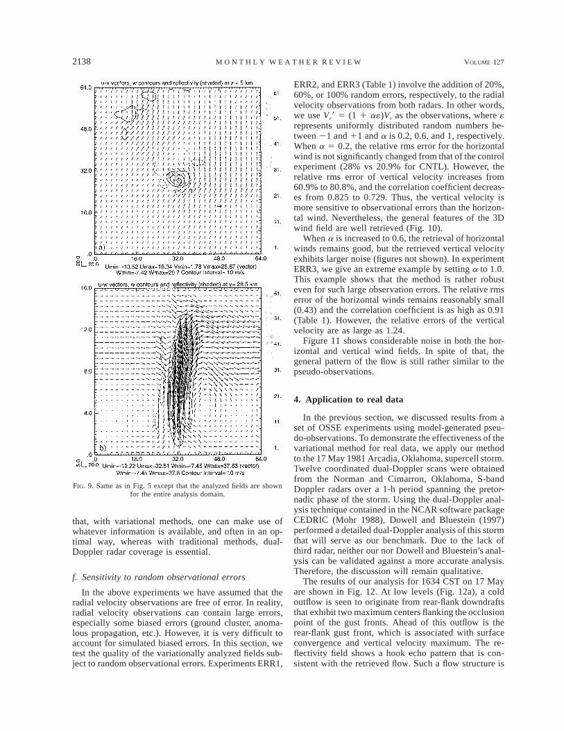
To examine the effectiveness of using a single sound-ing to specifying the background environment, we re-peat the control experiment without the backgroundsounding. The analyzed winds are plotted for the entiredomain in Fig. 8 and compared with those of the controlcase, replotted for the same domain in Fig. 9. In theanalysis without a background, no information is avail-able outside the data areas, the analysis remains largelyunchanged from the first guess, which in our case iszero (Fig. 8). However, for the control case, though noobservational constraint is available outside the radar-observed data areas, the analysis takes on the values ofthe background and the transition is smooth betweenthe data area and nondata area (Fig. 9). It is worth point-

ing out that even though the analysis outside the radardata areas is very poor with strong horizontal conver-gence and divergence near the data boundaries, the anal-ysis within the data coverage area is very good (cf. Fig.8 and Fig. 9). This again suggests that the current var-iational analysis is not very sensitive to data boundariesand parameters specified outside the radar-observedstorm region.

It is also interesting to note that near the northwestcorner of the domain, the left-moving storm is partiallycovered by a single radar (radar 2 in Fig. 2). Our analysisprocedure is still able to retrieve some of the flow struc-ture of this storm cell. This is possible due to the fact


FIG. 9. Same as in Fig. 5 except that the analyzed fields are shownfor the entire analysis domain.

that, with variational methods, one can make use ofwhatever information is available, and often in an op-timal way, whereas with traditional methods, dual-Doppler radar coverage is essential.

f. Sensitivity to random observational errors

In the above experiments we have assumed that theradial velocity observations are free of error. In reality,radial velocity observations can contain large errors,especially some biased errors (ground cluster, anoma-lous propagation, etc.). However, it is very difficult toaccount for simulated biased errors. In this section, wetest the quality of the variationally analyzed fields sub-ject to random observational errors. Experiments ERR1,

ERR2, and ERR3 (Table 1) involve the addition of 20%,60%, or 100% random errors, respectively, to the radialvelocity observations from both radars. In other words,we use Vr9 5 (1 1 a«)Vr as the observations, where «represents uniformly distributed random numbers be-tween 21 and 11 and a is 0.2, 0.6, and 1, respectively.When a 5 0.2, the relative rms error for the horizontalwind is not significantly changed from that of the controlexperiment (28% vs 20.9% for CNTL). However, therelative rms error of vertical velocity increases from60.9% to 80.8%, and the correlation coefficient decreas-es from 0.825 to 0.729. Thus, the vertical velocity ismore sensitive to observational errors than the horizon-tal wind. Nevertheless, the general features of the 3Dwind field are well retrieved (Fig. 10).

When a is increased to 0.6, the retrieval of horizontalwinds remains good, but the retrieved vertical velocityexhibits larger noise (figures not shown). In experimentERR3, we give an extreme example by setting a to 1.0.This example shows that the method is rather robusteven for such large observation errors. The relative rmserror of the horizontal winds remains reasonably small(0.43) and the correlation coefficient is as high as 0.91(Table 1). However, the relative errors of the verticalvelocity are as large as 1.24.

Figure 11 shows considerable noise in both the hor-izontal and vertical wind fields. In spite of that, thegeneral pattern of the flow is still rather similar to thepseudo-observations.

4. Application to real data

In the previous section, we discussed results from aset of OSSE experiments using model-generated pseu-do-observations. To demonstrate the effectiveness of thevariational method for real data, we apply our methodto the 17 May 1981 Arcadia, Oklahoma, supercell storm.Twelve coordinated dual-Doppler scans were obtainedfrom the Norman and Cimarron, Oklahoma, S-bandDoppler radars over a 1-h period spanning the pretor-nadic phase of the storm. Using the dual-Doppler anal-ysis technique contained in the NCAR software packageCEDRIC (Mohr 1988), Dowell and Bluestein (1997)performed a detailed dual-Doppler analysis of this stormthat will serve as our benchmark. Due to the lack ofthird radar, neither our nor Dowell and Bluestein’s anal-ysis can be validated against a more accurate analysis.Therefore, the discussion will remain qualitative.

The results of our analysis for 1634 CST on 17 Mayare shown in Fig. 12. At low levels (Fig. 12a), a coldoutflow is seen to originate from rear-flank downdraftsthat exhibit two maximum centers flanking the occlusionpoint of the gust fronts. Ahead of this outflow is therear-flank gust front, which is associated with surfaceconvergence and vertical velocity maximum. The re-flectivity field shows a hook echo pattern that is con-sistent with the retrieved flow. Such a flow structure is


FIG. 10. Same as in Fig. 5 but for experiment ERR1, which includesrandom observational errors up to 20% of the original values.

FIG. 11. Same as in Fig. 5 but for experiment ERR3, which includesrandom observational errors up to 100% of the original values.

typical of a tornadic supercell storm with strong low-level rotation (Lemon and Doswell 1979).

At midlevels, a strong updraft core (.25 m s21) isretrieved that is roughly collocated with the mesocy-clone (center of strong rotation) and reflectivity maxi-mum (Fig. 12b). In a vertical cross section plottedthrough the line A–B in Fig. 12a, the main updraft isseen to originate ahead of the low-level gust front. Itreaches a maximum intensity of 35.42 m s21 at the 8-kmlevel and in general matches the areas of maximumreflectivity. The main downdraft is located below theupdraft core and is collocated with a region of highreflectivity behind the gust front. These features suggestthat both the horizontal and vertical flows are kine-

matically consistent. They also qualitatively agree withthose analyzed in Dowell and Bluestein (1997).

5. Summary and concluding remarks

In this paper, we proposed and tested a variationalanalysis scheme that is capable of retrieving three-di-mensional winds from dual-Doppler observations ofconvective storms. It was shown that the variationalmethod has notable advantages over traditional dual-Doppler analysis techniques. The need for explicitly in-tegrating the mass continuity equations and solving el-liptic equations in the variational adjustment step, aswell as the ‘‘hole filling’’ procedure, makes the analysis


FIG. 12. Wind vectors and vertical velocity (contours) retrieved using the variational analysis method for the Arcadia, OK, 17 May 1981tornadic storm. (a) Horizontal cross section at z 5 0.5 km. (b) Horizontal cross section at z 5 5 km. (c) Vertical cross section through lineA–B in (a).

from traditional methods more susceptible to boundarycondition uncertainties than the variational method here.In addition, separate interpolation from radar observa-tion to an analysis grid in the traditional method is oftena source of errors.

The main conclusions can be drawn as follows:

R The new method incorporates the radar data, and

background fields, along with smoothness, mass con-tinuity, and possibly other dynamic constraints in asingle cost function. By minimizing this cost function,an analysis with the desired fit to these constraints isobtained in a single step.

R Because the method preserves the radial nature of theobservations, allowing for the backward interpolation


(from model grid to observation points) is used im-plicitly to keep the observations close to their ‘‘raw’’form.

R The method is flexible in handling other types of data.They can be either analyzed and forecast backgroundfields, or more conventional observations (e.g., sur-face mesonet, upper-air sounding and profile data).The use of a background naturally fills in the ‘‘holes’’of radar observations. The method has the additionalbenefit of being able to retrieve, with reasonable ac-curacy, the fields from single-Doppler data, extendingthe effective area of analysis beyond that of traditionalmethods.

R Because no explicit integration of the anelastic masscontinuity equation occurs, error accumulation duringthe integration is avoided. As a result, the method isalso less sensitive to boundary uncertainties.

R The method is robust enough to resist large randomobservational errors.

We plan to generalize our variational analysis pro-cedure to include additional data sources, and to intro-duce dynamic constraints in the cost function so thatthermodynamical fields are retrieved simultaneouslywith the winds. This procedure is expected to furtherimprove the wind analysis at the same time.

Acknowledgments. This research was supported byNSF Grant ATM91-20009 to the Center for Analysisand Prediction of Storms, by U.S. Department of De-fense (Navy) Grant N00014-96-1-112 to A. Shapirothrough the Coastal Meteorological Research Program.The first author appreciates the enlightening discussionswith Dr. Qin Xu at the Naval Research Laboratory. Spe-cial thanks go to Steve Weygandt for providing the Ar-cadia storm dataset, which came from Howard Bluesteinand David Dowell. Graphics plots were generated bythe ZXPLOT graphics package written by Ming Xue.Computations were performed on the Pittsburgh Su-percomputing Center Cray C90. Finally we would liketo thank three anonymous reviewers for their very help-ful comments that substantially improved the quality ofthis manuscript.

REFERENCES

Armijo, L., 1969: A theory for the determination of wind and pre-cipitation velocities with Doppler radars. J. Amos. Sci., 26, 570–573.

Atkins, N. T., T. M. Weckwerth, and R. M. Wakimoto, 1995: Ob-servations of the sea-breeze front during CaPE. Part II: Dual-Doppler and aircraft analysis. Mon. Wea. Rev., 123, 944–969.

Atlas, D., R. C. Srivastava, and R. S. Sekhon, 1973: Doppler radarcharacteristics of precipitation at vertical incidence. Rev. Geo-phys. Space Phys., 11, 1–35.

Brandes, E. A., 1977: Flow in severe thunderstorms observed by dual-Doppler radar. Mon. Wea. Rev., 105, 113–120.

Carbone, R. E., 1983: A severe frontal rainband. Part II: Tornadoparent vortex circulation. J. Atmos. Sci., 40, 2639–2654.

Chong, M., J. Testud, and F. Roux, 1983a: Three-dimensional windfield analysis from dual-Doppler radar data. Part II: Minimizing

the error due to temporal variation. J. Climate Appl. Meteor.,22, 1216–1226., , and , 1983b: Three-dimensional wind field analysisfrom dual-Doppler radar data. Part III: The boundary condition:An optimum determination based on a variational concept. J.Climate Appl. Meteor., 22, 1227–1241.

Cressman, G. W., 1959: An operational objective analysis system.Mon. Wea. Rev., 87, 367–374.

Doviak, R. J., P. S. Ray, R. G. Strauch, and L. J. Miller, 1976: Errorestimation in wind fields derived from dual-Doppler radar mea-surement. J. Appl. Meteor., 15, 868–878.

Dowell, D. C., and H. B. Bluestein, 1997: The Arcadia, Oklahoma,storm of 17 May 1981: Analysis of a supercell during torna-dogensis. Mon. Wea. Rev., 125, 2562–2582.

Ellis, S., 1997: Hole-filling data voids in meteorological fields. M.S.thesis, University of Oklahoma, 198 pp. [Available from BizzellLibrary, University of Oklahoma, Norman, OK 73019.]

Foote, G. B., and P. S. duToit, 1969: Terminal velocity of raindropsaloft. J. Appl. Meteor., 8, 249–253.

Gal-Chen, T., 1982: Errors in fixed and moving frame of references:Applications for conventional and Doppler radar analysis. J. At-mos. Sci., 39, 2279–2300.

Gao, J., J. Chou, and L. Zhi, 1995: A method for determining thespatial structure of meteorological variable from the temporalevolution of observational data. Chinese J. Atmos. Sci., 19, 113–125.

Gill, P. E., W. Murray, and M. H. Wright, 1981: Practical Optimi-zation. Academic Press, 401 pp.

Hoffman, R. N., 1984: SASS wind ambiguity removal by direct min-imization. Part II: Use of smoothness and dynamical constraints.Mon. Wea. Rev., 112, 1829–1852.

Kessinger, C. J., P. S. Ray, and C. E. Hane, 1987: The Oklahomasquall line of 19 May 1977. Part I: A multiple Doppler analysisof convective and stratiform structure. J. Atmos. Sci., 44, 2840–2864.

Kessler, E., 1969: On the Distribution and Continuity of Water Sub-stance in Atmospheric Circulation. Meteor. Monogr., No. 32,Amer. Meteor. Soc., 84 pp.

Klemp, J. B., and R. B. Wilhelmson, 1978: Simulations of right- andleft-moving storms produced through storm splitting. J. Atmos.Sci., 35, 1097–1110., and R. Rotunno, 1983: A study of the tornadic region withina supercell thunderstorm. J. Atmos. Sci., 40, 359–377., R. B. Wilhelmson, and P. S. Ray, 1981: Observed and numer-ically simulated structure of a mature supercell thunderstorm. J.Atmos. Sci., 38, 1558–1580.

Lemon, L. R., and C. A. Doswell, 1979: Severe thunderstorm evo-lution and mesocyclone structure as related to tornadogenesis.Mon. Wea. Rev., 107, 1184–1197.

Lhermitte, R. M., and L. J. Miller, 1970: Doppler radar methodologyfor the observation of convective storms. Preprints, 14th Conf.on Radar Meteorology, Tucson, AZ, Amer. Meteor. Soc., 133–138.

Lin, Y., P. S. Ray, and K. W. Johnson, 1993: Initialization of a modeledconvective storm using Doppler radar-derived fields. Mon. Wea.Rev., 121, 2757–2775.

Miller, L. J., and R. G. Strauch, 1974: A dual Doppler radar methodfor the determination of wind velocities within precipitatingweather systems. Remote Sens. Environ., 3, 219–235.

Mohr, C. G., 1988: CEDRIC—Cartesian Space Data Processor.NCAR, Boulder, CO, 78 pp.

Navon, I. M., and D. M. Legler, 1987: Conjugate-gradient methodsfor large-scale minimization in meteorology. Mon. Wea. Rev.,115, 1479–1502.

O’Brien, J. J., 1970: Alternative solutions to the classic vertical ve-locity problem. J. Appl. Meteor., 9, 197–203.

Parsons, D. B., and R. A. Kropfli, 1990: Dynamics and fine structureof a microburst. J. Atmos. Sci., 47, 1674–1692.

Ray, P. S., R. J. Doviak, G. B. Walker, D. Sirmans, J. Carter, and B.


Bumgarner, 1975: Dual-Doppler observations of a tornadicstorm. J. Appl. Meteor., 14, 1421–1530., C. L. Ziegler, W. Bumgarner, and R. J. Serafin, 1980: Single-and multiple-Doppler radar observations of tornadic storms.Mon. Wea. Rev., 108, 1607–1625., B. C. Johnson, K. W. Johnson, J. S. Bradberry, J. J. Stephens,K. K. Wagner, R. B. Wilhelmson, and J. B. Klemp, 1981: Themorphology of several tornadic storms on 20 May 1977. J. At-mos. Sci., 38, 1643–1663.

Reinking, R. F., R. J. Doviak, and R. O. Gilmer, 1981: Clear-air rollvortices and turbulent motions as detected with an air-borne gustprobe and dual-Doppler radar. J. Appl. Meteor., 20, 678–685.

Sasaki, Y., 1970: Some basic formalisms in numerical variationalanalysis. Mon. Wea. Rev., 98, 875–883.

Shapiro, A., and J. J. Mewes, 1999: New formulations of dual-Dopp-ler wind analysis. J. Atmos. Oceanic Technol., 16, 782–792.

Sun, J., and N. A. Crook, 1994: Wind and thermodynamic retrievalfrom single-Doppler measurements of a gust front observed dur-ing Phoenix II. Mon. Wea. Rev., 122, 1075–1091., and , 1997: Dynamical and microphysical retrieval fromDoppler radar observations using a cloud model and its adjoint.Part I: Model development and simulated data experiments. J.Atmos. Sci., 54, 1642–1661., and , 1998: Dynamical and microphysical retrieval fromDoppler radar observations using a cloud model and its adjoint.

Part II: Retrieval experiments of an observed Florida convectivestorm. J. Atmos. Sci., 55, 835–852.

Testud, J. D., and M. Chong, 1983: Three-dimensional wind fieldanalysis from dual-Doppler radar data. Part I: Filtering, inter-polation and differentiating the raw data. J. Climate Appl. Me-teor., 22, 1204–1215.

Thacker, W. C., 1988: Fitting models to inadequate data by enforcingspatial and temporal smoothness. J. Geophys. Res., 93, 10 655–10 665.

Xu, Q., and C. J. Qiu, 1994: Simple adjoint methods for single-Doppler wind analysis with a strong constraint of mass conser-vation. J. Atmos. Oceanic Technol., 11, 289–298.

Xue, M., K. K. Droegemeier, V. Wong, A. Shapiro, and K. Brewster,1995: Advanced Regional Prediction System (ARPS) version 4.0user’s guide. 380 pp. [Available from Center for Analysis andPrediction of Storms, University of Oklahoma, 100 E. Boyd,Norman, OK 73019.]

Yang, S., and Q. Xu, 1996: Statistical errors in variational data as-similation—A theoretical one-dimensional analysis applied toDoppler wind retrieval. J. Atmos. Sci., 53, 2563–2577.

Ziegler, C. L., 1978: A dual Doppler variational objective analysisas applied to studies of convective storms. M.S. thesis, Univer-sity of Oklahoma, 116 pp. [Available from Bizzell Library, Uni-versity of Oklahoma, Norman, OK 73019.], P. S. Ray, and N. C. Knight, 1983: Hail growth in an Oklahomamulticell storm. J. Atmos. Sci., 40, 1768–1791.

Documents

A Variational Method for the Analysis of Three …twister.caps.ou.edu/DualDoppler98/GaoDual1999.pdf2128 MONTHLY WEATHER REVIEW VOLUME 127 q 1999 American Meteorological Society A Variational