A Unified Theory of Attentional Control

Matthew H. Wilder, Michael C. Mozer and Christopher D. Wickens

mozer,wildermh@colorado.edu

Department of Computer Science and Institute of Cognitive Science

University of Colorado, Boulder, CO 80309-0430

University of Illinois, University of Colorado, and Alionscience: MA & D Operations

October 23, 2009

Abstract

Although diverse, theories of visual attention generally share the notion that attention is

controlled by some combination of three distinct strategies: (1) exogenous cueing from locally-

contrasting primitive visual features, such as abrupt onsets or color singletons (e.g., Itti et al.,

1998); (2) endogenous gain modulation of exogenous activations, used to guide attention to

task relevant features (e.g. Navalpakkam and Itti, 2005; Wolfe, 1994, 2007); and (3) endogenous

prediction of likely locations of interest, based on task and scene gist (e.g., Torralba, Oliva,

Castelhano, and Henderson, 2006). We propose a unifying conceptualization in which attention

is controlled along two dimensions: the degree of task focus and the spatial scale of operation.

Previously proposed strategies—and their combinations—can be viewed as instances of this

mechanism. Thus, this theory serves not as a replacement for existing models, but as a means

of bringing them into a coherent framework. We implement this theory and demonstrate its

applicability to a wide range of attentional phenomena. The model successfully yields the trends

found in visual search tasks with synthetic images and makes predictions that correspond well

with human eye movement data for tasks involving real-world images. In addition, the theory

yields an unusual perspective on attention that places a fundamental emphasis on the role of

experience and task-related knowledge.

1

1 Introduction

The human visual system can be configured to perform a remarkable variety of arbitrary tasks.

For example, in a pile of coins, we can find the coin of a particular denomination, color, or shape,

determine whether there are more heads than tails, locate a coin that is foreign, or find a combi-

nation of coins that yields a certain total. The flexibility of the visual system to task demands is

achieved by control of visual attention.

Three distinct control strategies have been discussed in the literature. Earliest in chronological

order, exogenous control was the focus of both experimental research (e.g., Averbach and Coriell,

1961; Posner and Cohen, 1984; Treisman, 1982) and theoretical perspectives (e.g., Itti and Koch,

2000; Julesz, 1984; Koch and Ullman, 1985; Neisser, 1967). Exogenous control refers to the guidance

of attention to distinctive, locally contrasting visual features such as color, luminance, texture, and

abrupt onsets. Theories of exogenous control assume a saliency map, a spatiotopic map in which

activation in a location indicates saliency or likely relevance of that location. Activity in the saliency

map is typically computed in the following way. Primitive features are first extracted from the visual

field along dimensions such as intensity, color, and orientation. For each dimension, broadly tuned,

highly overlapping detectors are assumed that yield a coarse coding of the dimension. For example,

on the color dimension, one might posit spatial feature maps tuned to red, yellow, blue, and green.

Next, local contrast is computed for each feature—both in space and time—yielding an activity

map that specifies distinctive locations containing that feature. These feature-contrast maps are

combined together to yield a saliency map. Saliency thus corresponds to all locations that stand

out from their spatial or temporal neighborhood in terms of their primitive visual features.

Attention need not be deployed in a purely exogenous manner but can be influenced by task

demands (e.g., Bacon and Egeth, 1994; Folk et al., 1992; Wolfe et al., 1989). The ability of in-

dividuals to attend based on features such as color or orientation has led to theories proposing

feature-based endogenous control (e.g., Mozer and Baldwin, 2008; Mozer, 1991; Navalpakkam and

Itti, 2005; Wolfe, 1994, 2007). In these theories, the contribution of feature-contrast maps to the

saliency map is weighted by endogenous gains on the feature-contrast maps, as depicted in Figure 1.

The result is that an image such as that in Figure 2a, which contains singletons in both color and

orientation, might yield a saliency activation map like that in Figure 2b if task contingencies involve

2

visual

saliencymap

verticalhorizontal green red

primitive-feature endogenous

exogenous activations

attentionalselection

attentionalstate

image gainscontrast maps

+

Figure 1: A depiction of feature-based endogenous control

(a) (b) (c)

Figure 2: (a) a display containing two singletons, one in color and one in orientation; (b) a saliency map ifcolor is a task-relevant feature; (c) a saliency map if orientation is a task-relevant feature

color or like that in Figure 2c if the task contingencies involve orientation.

Experimental studies support a third attentional control strategy in which attention is guided

to visual field regions likely to be of interest based on the current task and global properties of

the scene (e.g., Biederman, 1972; Neider and Zelinsky, 2006; Siagian and Itti, 2007; Torralba et al.,

2006; Wolfe, 1998a). This type of scene-based endogenous control seems intuitive: if you are looking

for your keys in the kitchen, they are likely to be on a counter. If you are waiting for a ride on a

street, the car is likely to appear on the road not on a building. Even without a detailed analysis

of the visual scene, its gist can be inferred—e.g., whether one is in a kitchen or on the street,

and the perspective from which the scene is viewed—and this gist can guide attention. Oliva and

Torralba (2001) show that scene identity can be inferred without any object information; a finding

that further supports the claim that scene-gist computation is an attentional process.

1.1 A Unifying Framework

Instead of conceiving of the three control strategies as distinct and unrelated mechanisms, a key

contribution of this work is to characterize the strategies as components of a broader control space.

As depicted in Figure 3, the control space spans two dimensions: task specificity and spatial scale.

Task specificity refers to the degree to which control exploits the current tasks and goals. High

task-specificity refers to situations in which the attentional system is strongly constrained by the

nature or properties of the task. Low task-specificity occurs in situations where the individual has

3

feature-basedendogenous

exogenous

scene-basedendogenous

Spatial ScaleTa

sk S

peci

ficity

local global

low

high

Figure 3: A two dimensional control space that characterizes exogenous, feature-based endogenous, andscene-based endogenous control of visual attention.

no particular goal or when attention operates in a task-independent manner. In this paper we

focus on visual search, and consequently, tasks can be defined in the currency of objects—i.e. a

search for a specific object or a class of objects. Within the context of visual search, high task

specificity refers to search for a particular object (e.g., a red bike), and low task specificity refers

to exploration in the absence of a particular goal.

In the control space, the spatial scale dimension is analogous to the granularity of image process-

ing. At the local scale, small regions in the image are processed separately and saliency predictions

for one region are roughly independent of the predictions for different region. Conversely, process-

ing at the global spatial scale is more holistic—general scene properties extracted from the entire

image are used to make saliency predictions across the whole field of view.

The two dimensions of the control space are helpful in explicating the similarities and differences

between the three control strategies we’ve described. Exogenous control appears in the lower left

corner of the space in Figure 3 because it operates independently of current goals and uses the local

spatial scale. Feature-based and scene-based endogenous control are placed in the upper region

of the space because both operate with a high degree of task specificity. However, they reside at

different points along the spatial scale continuum. Feature-based endogenous control classifies a

small region as salient if specific features are present in that location. Scene-based endogenous

control uses the whole image to determine the gist of the scene. When searching for a specific

object or group of objects, the gist is then used to differentiate regions of the scene by relevance.

What benefit is there to laying out the three strategies in this control space? The control space

4

offers us the means to reconceptualize attentional control by illuminating the relationships among

differing control strategies—highlighting the dimensions along which one strategy is similar to and

different from another. In doing so, the control space suggests additional strategies that might

be employed by attention. We return to this issue later, when we recharacterize other attentional

phenomena in terms of the control space.

1.2 Combining Control Strategies

We have argued for the existence of at least three distinct attentional control strategies which fit

into a control space (Figure 3) that varies with task-specificity and spatial scale of processing.

Given the possibility of distinct control strategies, one might ask how the strategies are employed.

A simple hypothesis is that control processes operate at a single point in the control space, and that

point is selected so as to optimize performance in a specific environment. If the selected point was in

between two of the primary strategies depicted in Figure 3, it might appear that multiple strategies

were operating simultaneously. Alternatively, multiple strategies might be employed in parallel,

and attention would be governed by some combination of or arbitration among the strategies.

Recently, several hybrid models have been proposed that incorporate multiple strategies oper-

ating in parallel. Torralba, Oliva, Castelhano, and Henderson (2006) present a model—which we

refer to hereafter as TOCH—that integrates object-specific scene-based endogenous control with

standard exogenous control. Navalpakkam and Itti (2005) combine exogenous with feature-based

endogenous control in a model we refer to as NI. In the upgrade of Guided Search to the current

4.0 version, Wolfe (2007) added bottom-up exogenous activation and scene-gist processing to the

existing feature-based endogenous control. Siagian and Itti (2007) propose an architecture—which

we call SI —that computes gist and exogenous saliency in parallel using the same biologically plau-

sible visual features. The exogenous component drives the saliency map but can be aided by the

gist information.

Most of these hybrid models combine task specific processing at the global spatial scale with

some form of processing at the local spatial scale. One advantage of the control space, however, is

that it suggests an even wider range of strategies to employ in guiding attention. In this paper, we

present a framework that encompasses any combination of strategies in the control space. We view

this framework as a generalization of earlier hybrid models such as TOCH, NI, Guided Search, and

5

SI.

In order to implement combinations of control strategies, we must be able to specify a control

strategy at any point in the space. We have a good understanding of how to implement the pri-

mary control strategies, which lie near corner of the space (depicted in Figure 3). An immediate

challenge, however, is to characterize the interior of the control space—what it means for a control

strategy to operate at an intermediate spatial scale and with an intermediate degree of task speci-

ficty. Parameterizing a model over a continuum of spatial scales seems straightforward, but how

would varying degrees of task specificity be implemented? To answer this question, it is useful to

digress and consider the role of experience in attention. By illuminating the relationship between

attentional strategies and experience, we formulate a novel hypothesis which strongly intertwines

attention and experience. This hypothesis offers a natural way to represent varying degrees of task

specificity.

1.3 Experience-based Attention

Consider the influence of experience on the three primary control strategies. Exogenous control

is typically envisioned as a hard-wired bottom-up process that is independent of an individual’s

experience. Experience plays a larger role in feature-based endogenous control: task instructions

or knowledge can modulate bottom-up processes to amplify task-relevant features. Nonetheless,

representations in the attentional system are still considered fixed and experience independent.

Scene-based endogenous control places a greater emphasis on experience. Performance in a partic-

ular environment—e.g., city streets, kitchens, etc.—depends on associations between coarse image

properties and scene types learned through experience.

These descriptions suggest that the influence of experience on attentional control varies depend-

ing on the specific strategy employed. In contrast to this classical view, we suggest here that all

attentional control strategies can be formally characterized as experience dependent.

We motivate this perspective with the observation that experience appears to have an effect

on attentional processes that are typically thought of as exogenous. For example, in figure-ground

assignment, Vecera et al. (2002) find that participants tend to select regions in the lower portion of a

synthetic black-white image as figure and regions in the upper portion of the image as background.

This result can be seen as a natural consequence of experience-based attention because individuals

6

have more experience attending to objects in the lower half of their visual fields. Peterson and Skow-

Grant (2004) provide another argument for the role of experience in figure-ground assignment by

showing directly that the choice of figure is biased by shape familiarity. For example, a sillouette

of a face is preferred as the figure over the anti-sillouette. Because figure-ground segregation is

generally considered an early, preattentive process, this work implicates experience as a factor that

affects attentional allocation.

In the domain of real-world images, Cerf et al. (2008b) offer stronger evidence for experience-

driven attention by comparing a standard exogenous model of attention with a new model that

combines the exogenous model with a face detection model. The authors find that the addition of a

face detection component significantly improves the correspondence between model predictions and

human eye-movements. Surprisingly, an improvement is found even for images that do not contain

faces. One interpretation of this result is that because faces are encountered frequently and are

usually relevant, the attentional system is tuned to report face-like regions as salient. In subsequent

work, Cerf et al. (2008a) show that comparisons to human eye-movements are even better when

more object models contribute to the final saliency map. These results imply that experience is an

important factor in attention even in free-viewing situations when no task is being performed.

Another argument for the fundamental role of experience in attention comes from adaptation

effects. Senders (1964) shows that fixation frequency to components in an instrument panel corre-

sponds to the bandwidth (events per second) of that component. Over days of training, participants

learned the statistics of the instrument panel and allocated their attention according to those statis-

tics. More recently, Geng and Behrmann (2005) find that locations with high spatial probability

play a more important role in attention. Essentially this work suggests that the attentional system

encodes information about the frequency of events in various locations. Chun and Jiang (1998)

show that individuals adapt to predictive spatial configurations in a contextual cueing paradigm.

On some trials in this type of experiment, displays are presented that have a repeated distractor

configuration that predicts the target location. Other trials have a random, nonpredictive distractor

configuration. Participants show faster response times for the repeated predictive displays versus

the nonpredictive displays, a result which implies that attention learns these configurations through

experience. In an interesting study combining chess and contextual cueing, Brockmole et al. (2008)

show that experience with chess significantly affects performance on the search task. The authors

7

present participants with chess board displays, half of which contain piece configurations that are

predictive of the target location. Both novice and expert participants exhibit the standard contex-

tual cueing improvement of response time, but chess experts improve more quickly and ultimately

attain faster response times than the novices. Although the fact that attention can be adaptive

does not imply that attention always adapts, the results summarized in this section suggest the

parsimonious view that attentional processes constantly adapt to the ongoing stream of experience,

and therefore, that attention should be viewed as fundamentally knowledge or experience based.

1.4 Reconceptualizing the Control Space

Adopting the perspective that all varieties of attentional control are fundamentally experience de-

pendent, we return to consider our control space (Figure 3), and in particular, the task-specificity

dimension. A control strategy that has a high degree of task specificity necessarily requires expe-

rience with the particular task. However, control strategies that have low task dependence (e.g.,

exogenous control) have traditionally been viewed in terms of hardwired bottom-up and experience

independent mechanisms. Suppose instead that we considered exogenous control as having a de-

pendence on a broad range of past experience, i.e., as depending on every task. A pure exogenous

control strategy would thus be cast as “identify as salient locations that are interesting based on

the combination of all past experience on a wide variety of learned tasks.”

With our focus on visual search, each specific task corresponds to a target object, e.g., car keys,

wallet, car, traffic light. The task specificity dimension can be recast in terms of the size of the

subset of objects that guide attention—with decreasing specificity as the set size increases. A high

degree of task specificity might correspond to a single target object, e.g., a car or a person. An

intermediate degree of task specificity might be thought of as search for a more general class of

object, e.g., the set of all objects that are wheeled vehicles or living things. And low task specificity

would simply include all objects with which one has had experience.

Defining exogenous attention in this manner is an extension of the concept presented in Cerf

et al. (2008a,b). This generalization implies that pure bottom-up attention does not exist as a

separate mechanism but is rather a special case of what has traditionally been viewed as top-

down attentional control. In line with this claim, Folk et al. (1992) have found that involuntary

attention capture is contingent on the attentional control settings. In a cueing paradigm, the

8

authors manipulate the property of the cue, abrupt onset or color discontinuity, so that in some

cases it’s consistent with the target property and in other cases it’s inconsistent with the target

property. They find that the cue only captures attention when the property of the cue matches the

defining property of the search task—thus supporting the notion that bottom-up capture is in fact

dependent on the task settings.

With our reconceptualization of task specificity, we can describe any control strategy via a set

of modules that specialize in particular targets. The modules must also be characterized in terms

of the other dimension of the control space—the spatial scale at which they operate. This set of

modules can be cast in terms of a dual to the control space, which we will call the module grid,

depicted in Figure 4. Like the control space, the module grid has two dimensions, but the dimensions

focus on implementation. The rows of module grid enumerate specific targets of attention, and the

columns specify an analog of spatial scale, which we call range of influence and explain shortly.

Each cell in the grid is a particular mechanism that produces a saliency map given a visual image.

Control strategies, which occupy a single point in control space (Figure 3), can occupy regions

in module grid (Figure 4). Exogenous attention corresponds to a short range of influence and a

combination across all targets. Feature-based endogenous attention also operates with a short range

of influence, but only a small collection of targets are employed—specifically those that contain the

defining features. Scene-based endogenous attentional guidance utilizes a long range of influence

and incorporates a small set of targets.

In reformulating the second dimension of the control space (Figure 3), a dimension analogous

to spatial scale is defined in the module grid—depicted along the columns of Figure 4. We describe

this dimension in terms of the spatial range of influence that a visual feature in the image has

on the saliency map. A short range of influence implies that saliency map activation at a given

location is determined only by nearby visual features, whereas a long range of influence implies that

activation anywhere in the saliency map can be influenced by features anywhere in the visual field.

Emphasizing the role of experience, the actual range of influence a visual feature will have depends

on statistics of the task environment and past experience: even if the potential connectivity is

present for long-range influences, the realization of these influences will depend on the particular

task environment, determined through experience.

Through experience, each module becomes specialized for a particular target. We’ve shown that

9

Range of Influence...

short long

person

car

house

tree

sign

light

Exogenous

Feature-basedEndogenous

Scene-basedEndogenous

Targ

et O

bjec

ts

Figure 4: A depiction of specific attentional mechanisms that are learned through experience. The twodimensions of this module grid relate to the nature of the experience and learning. This module grid canbe viewed as a transformation of the control space that emphasizes specific mechanisms and the role ofexperience. Each controls strategy—which corresponds to a point in control space—can be understood as acollection of grid squares in the module grid.

each primary strategy can be implemented as a subset of modules in one column of the module

grid. Similarly, the module grid can represent any combination of strategies in the control space if

multiple modules operate in parallel and their saliency maps are merged. We call this framework

TASC, an acronym on TAsk-specific and Spatial-scale Control. Rather than viewing TASC as an

alternative theory to existing models such as TOCH, Guided Search, and SI, we view TASC as a

generalization of these earlier theories, and each of these earlier theories can be seen as a specific

instantiation of TASC.

1.5 An Illustration of Saliency Over the Module Grid

To give a concrete intuition about the operation of TASC, we present an example illustrating the

model’s behavior. The input to TASC is an image—natural or synthetic—and the output from

TASC is a saliency map. TASC maintains a representation for each object target and range of

influence. Each representation yields a saliency map as shown in Figure 5 which corresponds

directly to the module grid in Figure 4. This example shows a street scene and the saliency maps

for three different objects: people, trees and sidewalks. In its full implementation, TASC would

maintain representations for a large collection of objects. At the short range of influence, saliency

maps generally make fine-grained predictions. These maps are similar to those obtained by feature-

10

pers

ontre

esi

dew

alk

longshort

Figure 5: A street scene and saliency maps produced by TASC in response to this input for three differenttarget objects and four ranges of influence.

based endogenous models like Guided Search 2.0. In contrast, the saliency maps from modules with

a long range of influence show coarse regions where the object is likely to appear.

As mentioned above, an advanced attentional strategy involves combining multiple modules

from the module grid. Figure 6a presents an example of a combined saliency map that could result

from TASC. This map is a combination across 11 objects and all ranges of influence. Figure 6b

shows separate saliency maps for each of the 4 ranges of influence where a combination is performed

across all 11 object modules. The map at the short range of influence corresponds to the exogenous

control strategy.

1.6 A Probabilistic Interpretation of TASC

Recent theories of visual attention have given a probabilistic interpretation to saliency (e.g. Bruce

and Tsotsos (2009); Gao et al. (2008); Kanan et al. (2009); Mozer et al. (2006); Mozer and Baldwin

(2008); Navalpakkam and Itti (2005); Torralba et al. (2006); Zhang et al. (2008)). In these theories,

11

(a) (b) (c)

longshort(d)

Figure 6: A saliency map (b) for the image in (a) using the naive control strategy in TASC—combine allmaps in the module grid. (c) the saliency map overlaid on the original image. (d) separate saliency mapsfor the 4 ranges of influence where all object modules are combined. These results come from a simulationwith 11 different target object representations.

saliency at some location x in the visual field is related to the probability that a target appears at

that location, P (Tx|Fx), where Tx is a binary random variable indicating the presence or absence of

a target at x, and Fx denotes the set of visual features on which the saliency assessment is based.

Each module of TASC further conditions on the object that is the goal of search, o, and the range

of influence, r: P (Tx|Fx, O = o,R = r). As we describe in the next section on implementation,

TASC uses a linear neural net to approximate this conditional probability. Any control strategy

involves combining the predictions of one or more modules. The combination rule can also be

expressed in probabilistic terms. To do so, we define the notion of a goal, G, that determines the

relative importance of individual objects and ranges of influence. That is, we define a conditional

distribution, P (O,R|G), that specifies for a given goal how likely a particular module is to be

important. One can integrate out over the uncertainty in this distribution:

P (Tx|G) =∑o

∑r

P (Tx|Fx, O = o,R = r)P (O = o,R = r|G).

We assume that P (O,R|G) has been learned through experience; however, we do not focus on this

form of attentional learning in the present paper. Given a specific goal, such as searching for a

person, P (O,R|G) will be peaked on a single target object and around ranges of influence that are

likely to be relevant. Given a more general goal, such as searching for a mode of transportation, the

12

probability mass in P (O,R|G) will be more widely distributed over objects. And given the most

general goal of all—to explore the visual environment—P (O,R|G) might either be based on priors

(i.e., by integrating out over the more specific goals), or might simply be uniform (i.e., all objects

and ranges are equally relevant). For simplicity we assume the latter in simulations of exogenous

control.

2 TASC Implementation

As with all models of attention, TASC assumes that computation of the saliency map can be

performed in parallel across the visual field with relatively simple operations. If computing saliency

was as computationally complex as recognizing objects, there wouldn’t be much use for the saliency

map because the purpose of the saliency map is to provide rapid heuristic guidance to the visual

system. In implementing TASC, each module from the module grid is configured to perform a

mapping from image to saliency map. The modules all have the same architecture, though they are

parameterized to implement varying ranges of influence, and the association from image to saliency

map is established via an object-specific training procedure which we describe shortly.

2.1 Overview of Processing Stages

Rather than creating yet another model of attention, our aim in developing TASC was to generalize

existing models such that existing models can be viewed as instantiations of TASC. Specifically,

the module processing mechanisms were chosen to be consistent with key implementation details

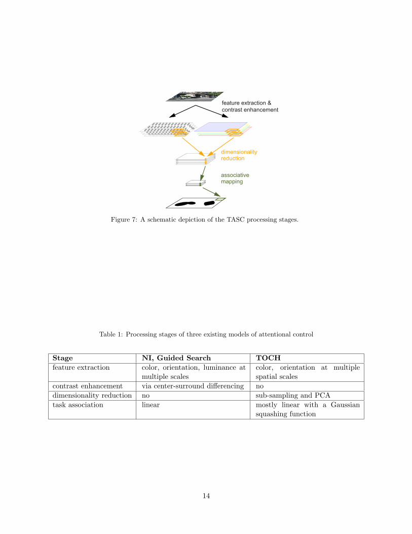
of several models including NI, TOCH, and Guided Search. Figure 7 provides a schematic depic-

tion of the TASC architecture. There are 4 main processing stages: feature extraction, contrast

enhancement, dimensionality reduction, and associative mapping. A subset of these stages is found

in most attention models. Table 1 lays out the basic processing stages used in NI, Guided Search,

and TOCH.

Image processing in TASC begins with a feature extraction stage in which raw pixel values are

converted into basic information about the presence of features including color and orientation. All

visual attention models that operate on raw image data use a similar form of feature extraction,

though some include other features such as luminance.

13

dimensionalityreduction

associativemapping

feature extraction &contrast enhancement

Figure 7: A schematic depiction of the TASC processing stages.

Table 1: Processing stages of three existing models of attentional control

Stage NI, Guided Search TOCHfeature extraction color, orientation, luminance at

multiple scalescolor, orientation at multiplespatial scales

contrast enhancement via center-surround differencing nodimensionality reduction no sub-sampling and PCAtask association linear mostly linear with a Gaussian

squashing function

14

Feature extraction is followed by a contrast enhancement stage that mimics neural processing

mechanism along the visual stream. This stage strengthens the response to regions that differ

significantly from their surround. TASC weights feature values by the ratio of center activity

to surround activity. NI implements contrast enhancement through center-surround differencing

across spatial frequencies and non-linear normalization. Contrast enhancement is not included in

TOCH.

The third processing stage is dimensionality reduction. Dimensionality reduction is used in the

scene gist computations in TOCH to limit the redundancy of the feature data. This reduction is

not necessary in NI and Guided Search because saliency predictions are based only on local feature

data which have a manageable dimensionality. Similar to TOCH, TASC uses sub-sampling and

principal components analysis to perform dimensionality reduction. The amount of reduction varies

with the module’s range of influence. At the short range of influence, significantly more feature

information is utilized across the whole image than at the long range of influence. This approach

matches the continuum seen between NI and TOCH.

The final processing stage involves constructing an object-specific saliency map from the di-

mensionality reduced image data. NI, Guided Search and TOCH are all attention models that can

be tuned to a specific search goal. In NI, linear weights for the individual feature channels are

learned from a set of test images related to the search task. Guided Search uses a set of linear

gains to modulate the weight of each feature channel. TOCH associates global features with likely

object locations through a weighted sum of linear regressors where the weights depend on the global

features in a non-linear way. Each module in TASC builds a linear mapping between feature values

and target locations for a specific object.

2.2 Patch Processing

For a given target object, we implement 4 TASC modules that have varying ranges of influence from

short to long. A specific range of influence is implemented by dividing the image into overlapping

patches of a specific size. Each image patch contributes only to the corresponding patch in the

saliency map. For modules with a short range of influence, small patches are used so that saliency

predictions are based only on local features—i.e. those within the small patch. At the longest

range of influence, the entire image is treated as a single patch which enables image features to

15

(a)

(b)

Figure 8: A depiction of patch processing for the 4 TASC modules that vary from short range of influence(left) to long range of influence (right). Each patch can only make predictions about its correspondingregion in the saliency map. Thus at the short range of influence, only local predictions are made. At thelong range of influence, however, image properties in any region can contribute to the saliency values in anyother region. In (b) see the saliency maps across the 4 ranges of influence for the image in (a) where thetask involves searching for trees. For all but the longest range of influence, patches are tiled such that theyoverlap by 50 percent.

have an effect on all saliency locations no matter how distant. The short range of influence modules

correspond well to the NI model whereas the long range of influence modules are more similar to

the global gist processing component of TOCH. Figure 8 shows a depiction of the patch sizes across

the 4 spatial scales. In this implementation we use square input images and square patch sizes

though this is not a requirement of the TASC framework. The model has 4 different patch sizes for

the 4 ranges of influence, φ1 = 1.56, φ2 = 6.25, φ3 = 25, and φ4 = 100 ordered from short to long

range of influence, where φ represents the percent of the image the patch spans. For each range of

influence, the image is tiled by patches that overlap by 50 percent.

Each TASC module processes the image in a patchwise fashion, with each patch processed

independently of each other. Patches are not recombined until the saliency map is formed. The

processing mechanisms are the same for all patches regardless of the range of influence, though

some processing parameters differ. Below we describe each processing mechanism and then present

the parameters that differ between ranges of influence.

16

2.3 Feature Extraction

TASC begins with an image such as in Figure 9a. From this image the model records feature

activations along 8 different channels: 4 color opponency and 4 orientation as shown in Figure 10a.

The value of each color channel is the difference between the RGB value for that color and its

opposing color (red opposes green and blue opposes yellow). All negative color feature values are

set to 0. If R,G,B are the pixel values and Y = (R + G)/2, then the red, green, blue and yellow

feature values are given by fr = max(0, R − G), fg = max(0, G − R), fb = max(0, B − Y ), and

fy = max(0, Y − B). Technically the feature values should be denoted R(x, y) and fr(x, y) for

each pixel location, (x, y), but we drop the location specification when it’s not necessary. For

the orientation channels, the intensity image is convolved with Gabor filters tuned to 4 different

orientations: 0, 45, 90, 135. All feature extraction parameters are the same across the 4 ranges of

influence.

The TASC feature extraction stage is very similar to feature extraction performed in the NI

and TOCH models. All models use the same process for extracting orientation values. NI uses

color opponency values similar to those used in TASC. In Itti and Koch (2000), which forms the

basis for the early stages of NI, two color channels are used: red-green and blue-yellow (negative

values allowed). TASC uses these same values but divides them into 4 channels to avoid negative

feature values.

The primary difference between feature extraction in TASC and the NI and TOCH models is

that TASC does not extract features at multiple spatial frequencies. Feature extraction utilizing

multiple spatial frequencies, obtained for example through the steerable pyramid (Simoncelli and

Freeman, 1995), is typically employed to improve the model’s ability to handle image datasets with

a diverse range of object and scene scales. To reduce the computational load, we chose to perform

feature extraction at a single spatial frequency in TASC and found the results satisfactory for our

simulations. Nevertheless, we envision a complete implementation of TASC that includes feature

extraction at multiple spatial frequencies and expect that this addition would improve the overall

performance.

17

(a) (b)

Figure 9: An example image, (a), and the saliency maps, (b), for the four ranges of influence from short tolong(left to right). Here the task is to search for the trees in the image.

(a) (b)

Figure 10: Activities in TASC for the first two stages of processing: feature extraction (a) and contrastenhancement (b). The original image is shown in Figure 9a. The feature channels on top are red, green,blue and yellow. The four channels on the bottom correspond to orientations of 0, 45, 90, and 135 degreesfrom left to right.

2.4 Contrast Enhancement

Contrast enhancement is implemented in TASC by weighting each feature value by the ratio of

center activity to surround activity (the result of which is shown in Figure 10b). The model

computes center and surround activity by convolving the feature data for each channel by two

gaussian kernels. Both kernels have a peak of 1 but they differ in their standard deviation, with σc

corresponding the center kernel and σs to the surround kernel. For each pixel and feature channel,

the model obtains a center value, cent, which measures the amount of activity close to that pixel

location and a surround value, surr, that measures the activity over the wider region surrounding

the location. The contrast value, c(x, y), is computed for each of the 8 feature channels as follows

using the red feature channel as an example:

cr(x, y) =centr(x, y)surrr(x, y)

fr(x, y),

18

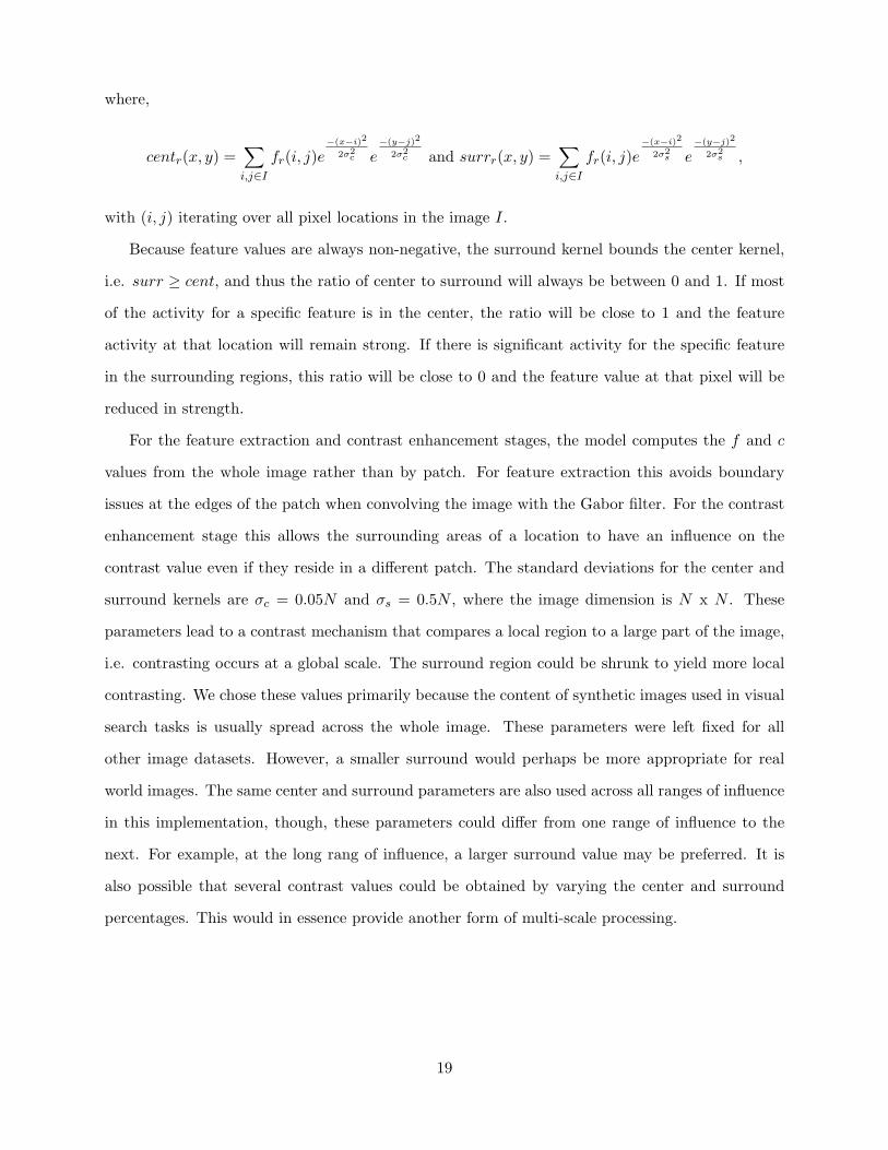
where,

centr(x, y) =∑i,j∈I

fr(i, j)e−(x−i)2

2σ2c e

−(y−j)2

2σ2c and surrr(x, y) =

∑i,j∈I

fr(i, j)e−(x−i)2

2σ2s e

−(y−j)2

2σ2s ,

with (i, j) iterating over all pixel locations in the image I.

Because feature values are always non-negative, the surround kernel bounds the center kernel,

i.e. surr ≥ cent, and thus the ratio of center to surround will always be between 0 and 1. If most

of the activity for a specific feature is in the center, the ratio will be close to 1 and the feature

activity at that location will remain strong. If there is significant activity for the specific feature

in the surrounding regions, this ratio will be close to 0 and the feature value at that pixel will be

reduced in strength.

For the feature extraction and contrast enhancement stages, the model computes the f and c

values from the whole image rather than by patch. For feature extraction this avoids boundary

issues at the edges of the patch when convolving the image with the Gabor filter. For the contrast

enhancement stage this allows the surrounding areas of a location to have an influence on the

contrast value even if they reside in a different patch. The standard deviations for the center and

surround kernels are σc = 0.05N and σs = 0.5N , where the image dimension is N x N . These

parameters lead to a contrast mechanism that compares a local region to a large part of the image,

i.e. contrasting occurs at a global scale. The surround region could be shrunk to yield more local

contrasting. We chose these values primarily because the content of synthetic images used in visual

search tasks is usually spread across the whole image. These parameters were left fixed for all

other image datasets. However, a smaller surround would perhaps be more appropriate for real

world images. The same center and surround parameters are also used across all ranges of influence

in this implementation, though, these parameters could differ from one range of influence to the

next. For example, at the long rang of influence, a larger surround value may be preferred. It is

also possible that several contrast values could be obtained by varying the center and surround

percentages. This would in essence provide another form of multi-scale processing.

19

2.5 Dimensionality Reduction

After the contrast enhancement stage, TASC maintains 8 feature values per pixel. For a patch with

many pixels, the dimensionality of this data is too high for most desired computations. Following

the methods used in TOCH for gist processing, the dimensionality is reduced significantly through

sub-sampling and principal components analysis while key information needed for classifying scenes

is still preserved.

2.5.1 Sub-sampling

As in TOCH, TASC uses a simple sub-sampling scheme where each pixel in the sub-sampled image

represents the mean value of all pixels in a corresponding unique, non-overlapping rectangular

region in the original data. Sub-sampling is performed only within feature channels so for each

sub-sampled region in the image the model still maintains 8 feature values. If the original patch

dimension is n x n and patches are sub-sampled the by a factor ρ, the new patch dimension becomes

n/ρ x n/ρ. Each pixel in the sub-sampled data corresponds to the average of all pixels in a ρ x ρ

block in the original data.

The extent of sub-sampling varies across ranges of influence in TASC. In essense more sub-

sampling is needed for the longer ranges of influence because the patches are larger and contain

more feature data. This approach fits well with both NI and TOCH. Specifically, NI operates

with a short range of influence and does not perform any sub-sampling while TOCH operates at a

long range of influence and consequently uses significant sub-sampling of feature data. The model

uses the following values of ρ for the four ranges of influence from short to long: ρ1 = 4, ρ2 = 8,

ρ3 = 8, and ρ4 = 16. These specific values were chosen to yield a reasonable computational load

in the following principal components analysis stage. However, changing these values does not

significantly affect the model’s performance.

2.5.2 Principal Components Analysis

After sub-sampling, the model uses principal components analysis (PCA) to further reduce the

dimensionality of data. This process extracts the critical feature properties of a patch and discards

extraneous feature information. PCA analysis is done separately for each of the 8 feature channels

20

and 4 ranges of influence. For each feature channel, the top ` principal components are preserved.

The PCA projections are derived from a set of patches extracted from our image database—using

several randomly distributed patches per image. The database contains roughly 2,500 images

including many varied real-world scenes and some synthetic visual search images. Note that for

a given feature channel and range of influence, the same PCA projection is used for all patches,

thus yielding a location independent reduction. Additionally, the same PCA projections are used

across all simulations described in the results section (including images with artificial displays and

real-world scenes).

We chose to perform PCA on each feature channel to preserve an equal amount of information

across all feature dimensions. The alternative would involve lumping all feature data together and

performing one PCA projection. In this case, PCA may find that a particular feature dimension

does not have significant discrimination power and thus would not maintain any information about

this feature channel in the top principal components. This could be problematic for visual search

tasks where the discarded feature plays a defining role. This problem could be avoided by carefully

controlling the database used for deriving the PCA projections, however, we found it preferable to

instead treat the individual feature channels independently.

If the original patch size is n x n, the dimensionality of each feature channel after subsampling

is (n/ρ)2. After PCA, there are only ` data points per channel. The full patch data, x, are obtained

by concatenating the data from each feature channel into a vector with dimensionality 8`. The

number of principal components used varies across the ranges of influence; from short range to

long range, `1 = 1, `2 = 3, `3 = 9, and `4 = 27. Because there are far more patches per image at

the shorter ranges of influence, the total number of data points per image decreases as the range

of influence becomes longer. At the shortest range of influence, there are 15x15=225 patches per

image (this number is odd because patches overlap). At progressively longer ranges of influence,

there are 7x7=49, 3x3=9, and 1x1=1 patches per image. From short to long range of influence, the

total data points used per image are 225x8x1=1800, 49x8x3=1176, 9x8x9=648, and 1x8x27=216

(patches x features x `).

Figure 11 provides an informative view into how the PCA stage functions by depicting which

regions each principal component favors for each feature channel. Each box in this figure displays

the values of a specific principal component vector for a specific channel. Lighter values correspond

21

red green blue yellow 0 45 90 135

Figure 11: Reconstructed principal component weights for the 8 feature channels. The top row correspondsto the first principal component. See text for more detailed explanation.

to stronger weights for the features at that location in the patch. Principal components decrease

in importance from top to bottom. The first principal component typically represents the DC level

of activity. Subsequent principal components provide more fine-grained spatial selectivity. The

principal component vectors reconstructed in this figure correspond to the second longest range

of influence for which 9 principal components are used. The PCA projections used for the other

ranges of influence exhibited a very similar pattern.

Figure 12 shows the representation for the image in Figure 9a after sub-sampling and PCA

at the 4 ranges of influence. Each row in Figures 12a-c shows 8 composite images, one for each

feature channel, formed by assembling the nth principal component value for each patch. The

top row corresponds to the first principal component and lower rows display subsequent principal

components with decreasing significance. Figure 12a is the representation for the shortest range

of influence. At the longest range of influence, Figure 12d, there is only one patch per image but

more principal components (now shown along the columns).

2.6 Task Associations and Learning

To implement modules that specialize for a variety of target objects, each module has a unique

collection of patch specific neural networks that link image features to object locations. Figure 9b

shows the output from an association network tuned to trees for the 4 ranges of influence. These

22

(a)

(b)

(c)

(d)

Figure 12: PCA activities in TASC at the four ranges of influence (shortest (a) to longest (d)) correspondingto the image in Figure 9a. A separate representation is maintained for each feature channel (here the orderingis: red, green, blue, yellow, 0, 45, 90, 135). PCA is computed at the patch level. Each block in these figurescorresponds to a PCA value for a specific feature channel and patch. At the shortest range of influence thereare 15x15 patches. At the longest range of influence, there is only one patch per image. In (a) – (c) the mostimportant component is in the top row and less important components are in lower rows. In (d) the principalcomponents decrease in importance from left to right. Lighter values correspond to greater activation.

23

are the final saliency maps for each module have been smoothed with a Gaussian filter.

For each patch in our image, there is set of input units representing the patch data, xp, after

dimensionality reduction. Each set of input units is fully connected to a set of output units via a

linear mapping. To limit the capacity of this network, we restrict the rank of the linear mapping.

This is equivalent to adding a hidden layer with a limited number of units. For each range of

influence, the number of hidden units is restricted to a different r < 8`. If the input to hidden

weight matrix for a patch is Vp and the hidden to output matrix is Wp, the linear mapping from

input to output, VpWp, has rank r. The model uses r1 = 1, r2 = 3, r3 = 9, and r4 = 27 for the 4

ranges of influence from short to long. This leads patches at the shorter range of influence to have

weaker descriptive ability. However, because there are far more patches at the shorter range of

influence, the module as a whole maintains adequate descriptive power. The output values for each

patch, op, are obtained by passing the output activations, xpVpWp, through the logistic sigmoid

function to yield meaningful saliency values between 0 and 1. For computational purposes, we

constrain the dimension of op to be smaller than the original patch dimensions because saliency

predictions do not need to be as fined grained as the original pixel information. The reduction is

such that the final saliency map has 32x32 pixels.

To obtain the final saliency map, the outputs from the individual patches must be combined.

Because the patches overlap, multiple output units can correspond to the same region in the

complete saliency map. Over most of the image, 4 overlapping patches contribute to a single

location, though, along the edges only 2 patches contribute and in the corners only one patch is

present. The final saliency value for a particular location, s(x, y), is computed as an average of all

patch output values at that location:

s(x, y) =1

|Ω(x, y)|∑

p∈Ω(x,y)

op(gp(x, y)),

where Ω(x, y) is the set of patches that contribute to point (x, y) in the saliency map, |Ω(x, y)| is

the cardinality of that set, and gp(x, y) is a function that maps the coordinates in the saliency map

to patch coordinates for a particular patch p.

To train a network for a specific task, we use a supervised learning approach based on the

LabelMe image database (Russel et al., 2008), which contains images labeled by pixel according

24

Figure 13: (above) Two images from the LabelMe database, (below) pixel-by-pixel labeling of three objects—cars (red), people (green), and buildings (blue).

to the object present at that corresponding location. Figure 13 shows two labeled images used for

training with cars, people, and buildings labeled (note that objects are sometimes not labeled).

Typically, our training sets for each object consist of 500-1000 images. During training, each image

is presented to the model, the model computes a dimensionality reduced feature representation

for each patch, and this representation serves as input to the patch specific neural network. Each

network is trained with a target output containing values of 1 at all locations in the patch where a

given target object appears and 0 at all other locations. Training is performed in batches using the

back propagation algorithm to update weights. Training continues until a local optimum in error

is obtained.

2.7 Combining Multiple Modules

So far we have discussed how each module in the module grid computes a saliency map for a specific

image. Each individual module could be used to guide attention. However, to implement more

complex strategies, such as hybrid models like TOCH, it is necessary to combine the saliency maps

from a collection of modules. It is this combination of modules that gives the TASC framework

its ability to model attentional guidance that varies in task specificity and utilizes multiple spatial

scales.

Several different approaches are possible for combining the saliency maps from multiple modules.

As we suggested in the introduction, a probabilistic approach could assign a prior probability to

the relevance of each module for a specific goal. The combination could then integrate out over

25

the uncertainty in the relevance of the modules, essentially computing a weighted summation of

module outputs, where the weights correspond to the module’s prior probability. One problem

with this probabilistic rule is that it can yield the same result when one module is highly active

at a location as it it would if many modules were modestly active at that location. If the module

with high activity is relevant to the goal, we’d intuitively expect the saliency at that location to

be high regardless of how the other modules respond. This observation suggests an alternative

approach to combining modules in which a subset of relevant modules is selected and the final

saliency value at a specific location corresponds to the maximum value at that location across the

subset of modules. This approach can be thought of as performing a disjunction across object

modules whereas the previous combination rule is more of a conjunction of modules. These two

approaches will produce similar results for highly constrained tasks because in the probabilistic

combination most of the mass of the distribution over modules will be concentrated on one module

and in the max combination the set of relevant modules will be small. When tasks become less

constrained, however, the predictions of these models become more different. We implemented both

combination rules in TASC and found that the max rule produced saliency maps that were more

consistent with experimental results. This second strategy was used for all simulations presented

in the results section.

Combining visual information using a max rule is not new in the literature. Zhaoping and Snow-

den (2006) propose a selection process that computes the maximum over feature maps. Riesenhuber

and Poggio (1999) argue for a max-like combination of different feature detectors in their object

recognition model. Evidence for max rule combinations can also be found at the neural imple-

mentation level of analysis. Specifically, Gawne and Martin (2002) and Lampl et al. (2004) find

examples of max operations occuring in monkey and cat visual corticies. The general finding is

that activities of objects in multiple locations (within one receptive field) lead to an activation level

in the visual cortex that is most similar to the max of the individual object activations when they

are presented separately. An intuitive argument can also be made for applying the max rule in

real-world situations. For example, if attention is tuned to search for wheeled vehicles and the car

module gives a strong response at a location, then that location should be salient even if the bike,

truck, bus, train, cart, and scooter modules all have a weak response at that location.

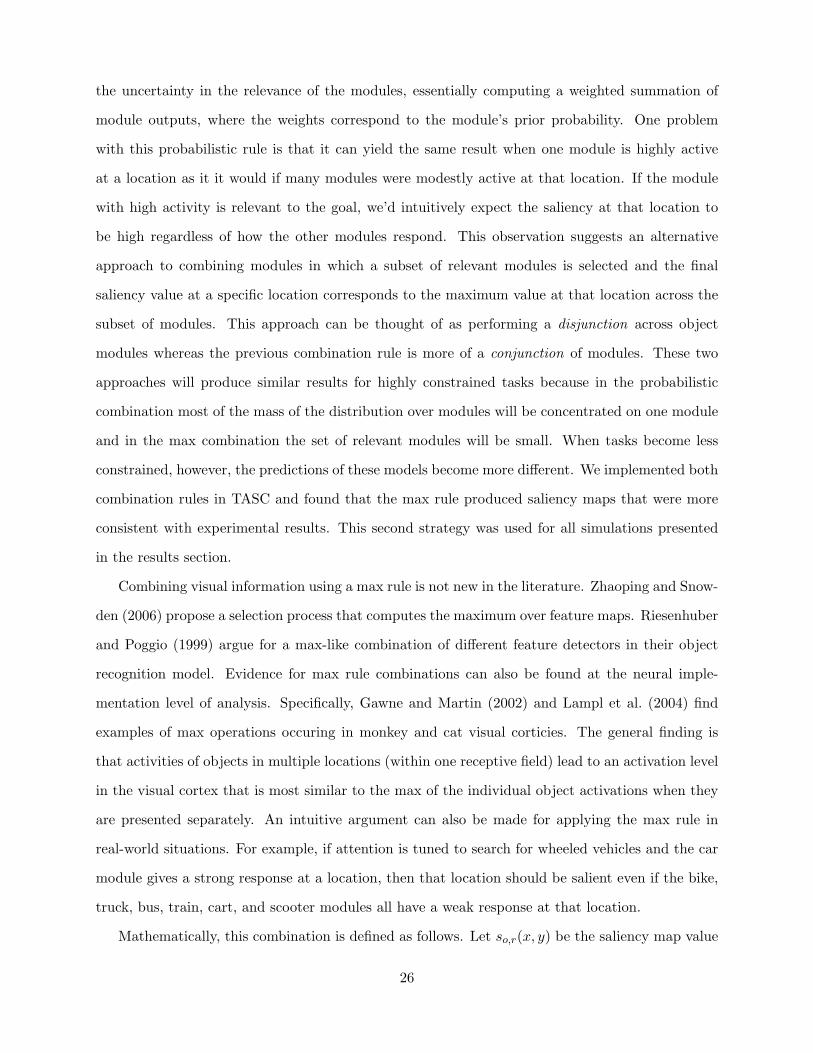
Mathematically, this combination is defined as follows. Let so,r(x, y) be the saliency map value

26

for target object o and range of influence r at location (x, y). The values in the combined saliency

map are given by

sc(x, y) = maxo,r∈M

so,r(x, y),

where M is the set of modules relevant to the current goal. In each of the simulations presented

in the next section, M is selected to fit the constraints of the search task. In most cases, M

contains modules associated with one specific target object, though at times the model combines

across multiple target objects. One can imagine that one range of influence might be more relevant

than another for a specific viewing goal, however, it is unclear how to select a subset of ranges for

that goal. Consequently, the model employs the most general strategy in all simulations, using all

ranges of influence for the relevant target objects. For free viewing simulations, i.e. pure exogenous

control, M contains every module in the module grid.

2.8 Key Components of the Implementation

At this point the model may seem rather complex in the number of stages to process an image

and obtain a saliency map. However, most of these components are present in existing attentional

models and don’t significantly contribute to the characteristics of TASC. Nevertheless, there are

several implementation decisions in TASC that are particularly important in defining the behavior

of the model. The feature extraction and contrast enhancement stages are mostly standard though

we prefer our specific implementation of contrast enhancement. For the PCA stage, we find it

important to reduce the dimensionality of the feature channels independently rather than operating

on all the data at once. This enables a high degree of reduction while ensuring that all feature

channels maintain an equally informative representation. Another key implementation decision is

the choice to restrict the association network to be linear. Linearity limits the complexity of the

mappings that can be learned and causes the model to perform a quick and dirty sort of object

recognition (we return to this point in the discussion). The final implementation decision that is

important in TASC is the use of the max of disjunction rule when combining modules. Another

point about this implementation worth mentioning, though not a specific design decision, is that

the same model is used for all simulations and the only difference from one simulation to the next

is the subset of modules used to obtain the final saliency map.

27

3 Simulation Results

Having explained our implementation of TASC, we now present simulations that demonstrate that

TASC accounts for a diverse set of findings in the attentional literature. We begin by testing

the model on classic visual search tasks. Next, we explore the contextual cueing paradigm and

observe how the TASC framework allows for the type of global contextual priming observed in

these experiments. We discuss how TASC provides an integrative framework that accomodates

other attentional phenomena including probabilistic spatial cueing and figure-ground assignment.

We conclude by testing TASC on real-world images and comparing the saliency predictions to eye-

movement data from human observers. In all these simulations, TASC operates on raw pixel images.

Historically, attentional models that simulate psychological findings used as input an abstract data

structure representing presegmented features. Here, we present a single model that uses the same

input representation for both artificial and real-world images.

3.1 Visual Search

Visual search tasks require that an individual detect a target element in a display surrounded by

distractor elements. Visual search is one of the most extensively studied tasks in the psychological

literature (see Wolfe (1998b) for a meta-analysis of a wide range of visual search experiments and

Wolfe and Horowitz (2004) for a review of the attributes that guide attention). The seminal work

of Treisman and Gelade (1980) revealed what appeared to be a fundamental dichotomy between

feature and conjunction search. In feature search, the target differs from all distractors along

a single feature dimension; for example, the target is red and the distractors are green (see the

display at the left of Figure 14a). In conjunction search, the target is defined by a conjunction

of features, and shares one feature in common with each distractor; for example, the target is

a red vertical bar among distractors that are green verticals or red horizontals (see Figure 14b).

Feature search is efficient in that search time is not dependent on the number of distractors in

the display; conjunction search is inefficient, due to the increased confusability between targets

and distractors. Any account of visual search needs to start by explaining the distinction between

feature and conjunction search. This explanation is a necessary but not sufficient condition for the

plausibility of a theory. The dichotomy between feature and conjunction search has given way to

28

Sing

le F

eatu

reC

onju

nctio

nO

ddba

ll

Short LongRange of Influence

(a)

(b)

(c)

Figure 14: Saliency maps at 4 ranges of influence for three different visual search paradigms: (a) featuresearch—a single red target among green distractors, (b) conjunction search—a single red vertical amonggreen verticals and red horizontals, and (c) oddball search—a singleton exists in each image but the specificfeatures of the target and the defining feature dimension are unknown before the trial.

many subtleties and quirks that populate the literature. Our goal in this work is not to explain

visual search in all its detail, but to demonstrate that TASC is a plausible candidate to tackle the

visual search literature.

In addition to the feature and conjunction search paradigms, we also explore oddball detection

or pop-out search. In an oddball-detection task, the target differs from distractors along one feature

dimension, but the feature dimension and the target feature value is not specified in advance of a

trial. For example, the participant might be required to find a red target among green elements,

a green element among red, a vertical among horizontals, or a horizontal among verticals (see the

display in Figure 14c). The target feature changes from trial to trial and thus part of the task

involves determining the relevant discrimination on the current trial.

To model visual search, we construct displays that contain elements varying along two feature

dimensions, color and orientation. To assess search performance, we require a measure of response

latency to detect a target as a function of the number of distractors in the display. (The efficiency

of search is reflected in the slope of this curve.) How are TASC’s saliency maps translated into

response latencies? We adopt an assumption from Guided Search 2.0 (Wolfe, 1994) regarding how

the saliency map is used in search. Guided Search supposes that display locations are examined

in order from most salient to least, and that response latency increases linearly with the number

of display locations examined. To compute the saliency rank of a display element, a Gaussian

29

filter is first applied to smooth the saliency map. The maximum saliency value in the immediate

region of the display element is then determined, and elements are ranked by saliency. One does

not need to assume serial search to obtain response latencies monotonic in saliency ranking. For

example, Guided Search 4.0 (Wolfe, 2007) proposes that saliency ranking determines the order in

which display locations are fed into a parallel but capacity limited asynchronous diffusion process

that performs object recognition. Under this assumption, response latency is affected not only by

saliency ranking but also by drift rates. Nevertheless, in the absense of familiarity differences among

the display elements, the capacity-limited parallel diffusion process roughly produces latencies

proportional to saliency ranking. One could embellish TASC to use the response accumulation

mechanism of Guided Search 4.0, but doing so would add little to the key results we present here.

Most visual search experiments include both target present and target absent trials. Target

absent displays provide insight into how search is terminated. Latencies are slower in target absent

trials but usually have a similar dependence on the number of distractors as in target present trials

for the same task. Search termination is not implemented in TASC for target absent trials and

the target rank measure is undefined for images that do not contain a target. Consequently, all

subsequent visual search simulations contain only target present trials.

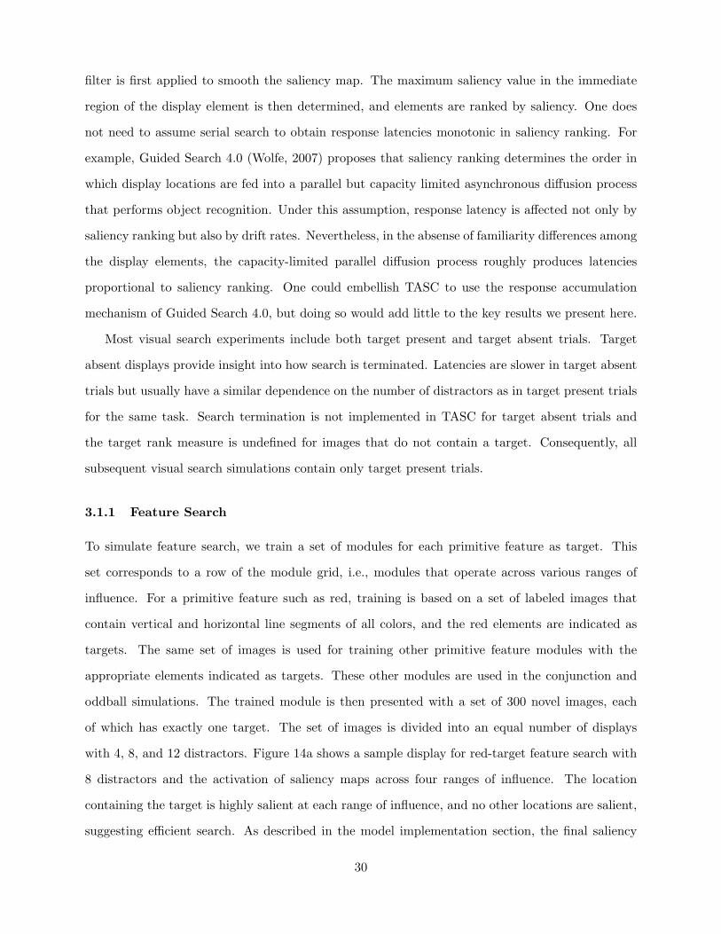
3.1.1 Feature Search

To simulate feature search, we train a set of modules for each primitive feature as target. This

set corresponds to a row of the module grid, i.e., modules that operate across various ranges of

influence. For a primitive feature such as red, training is based on a set of labeled images that

contain vertical and horizontal line segments of all colors, and the red elements are indicated as

targets. The same set of images is used for training other primitive feature modules with the

appropriate elements indicated as targets. These other modules are used in the conjunction and

oddball simulations. The trained module is then presented with a set of 300 novel images, each

of which has exactly one target. The set of images is divided into an equal number of displays

with 4, 8, and 12 distractors. Figure 14a shows a sample display for red-target feature search with

8 distractors and the activation of saliency maps across four ranges of influence. The location

containing the target is highly salient at each range of influence, and no other locations are salient,

suggesting efficient search. As described in the model implementation section, the final saliency

30

(a)4 8 12

1

2

3

4

5

Mea

n Sa

lienc

y R

ank

Number of Distractors

Single Feature

(b)4 8 12

1

2

3

4

5

Mea

n Sa

lienc

y R

ank

Number of Distractors

Conjunction

(c)4 8 12

1

2

3

4

5

Mea

n Sa

lienc

y R

ank

Number of Distractors

Oddball

Figure 15: The mean target ranking for three visual search simulations in TASC grouped by the numberof distractors in the display. Here we take target ranking to be proportional to response time. The task in(a) involves searching for a target defined on one feature dimension (i.e. find the red object amongst greendistractors). As expected, the target rank is independent of the number of distractors. (b) results for a classicconjunction task (i.e. search for red vertical bars amongst green vertical and red horizontal bars). Here theranking increases with the size of the distractor set suggesting that search is inefficient. (c) results for anoddball detection task where the target is a singleton along one dimension, but which dimension is unknownbefore the trial. As expected, response times for this task are independent of the number of distractors. Ingeneral, predicted response latencies in oddball detection tasks are slower than in single feature search.

map used to evaluate performance for each image is a combination of the four ranges of influence

shown in Figure 14a. It is clear that the target rank in the combined saliency map for this image

is 1. Figure 15a shows the mean target ranking across all 300 images grouped by display size.

Regardless of the number of distractors in the display, TASC obtains a saliency ranking of 1 for the

target element, suggesting a fast response time that is independent of display size, consistent with

behavioral studies showing efficient feature search. Feature search is efficient in TASC because the

contrast enhancement stage strengthens the target feature value and the neural net only activates

regions that contain the target feature. The target feature in this simulation was red, however, the

same result was obtained for green, blue, vertical, and horizontal targets.

Although TASC is trained to perform feature search, the model is agnostic as to whether this

training corresponds to experience within an individual’s lifetime, or experience on an evolutionary

time scale. The main claim of the model is that feature search is not special; it relies on the same

processing mechanisms as any other search task.

31

3.1.2 Conjunction Search

In principle, TASC could implement conjunction search in two different ways. First, saliency of a

conjunction target could be defined as the combination of the saliency maps of the two primitive

feature modules that make up the conjunction, i.e., saliency of red as target and saliency of vertical

as target. The combination of red and vertical maps would be no different than the combination

of automobile and bicycle maps when the target was a wheeled vehicle. Alternatively, a set of

specialized modules could be trained on the conjunction target—e.g., a module for red vertical

targets—treating the conjunction just like any more complex object like a car or person. The

semantics of the two alternatives are somewhat different: the combination of primitive feature

modules detects red or vertical, whereas the specialized conjunction module should in principle

detect red and vertical.

The saliency maps in Figure 14b were obtained from a simulation using the first approach—i.e.

representing conjunction as the combination of two primitive features. As the figure illustrates, the

saliency maps for a conjunction of features have significant spurious activation. Locations in which

red items are present are salient, as are locations in which verticals are present. The exact pattern

of activity depends on the configuration of elements, because the contrast and dimensionality

reduction stages of the model depend on the local configurations. In contrast to the situation

with feature search, the target does not stand out in the saliency map. Figure 15b shows that

the saliency rank of the target increases steeply with the number of distractors in the display,

suggesting that TASC has inadequate computational power to reliably detect a conjunction target.

Note that the saliency activation map is not random. If it were random, then the mean rank would

on expectation be half the number of items in the display—2.5, 4.5, and 6.5 for displays with 4, 8,

and 12 distractors, respectively. The observed rankings are better, indicating that some information

about the conjunction is available to the model. This occurs simply because on expectation, the

saliency of a red vertical element should be higher than an element that is just red or just vertical.

A key reason why TASC is inefficient on conjunction search is that saliency maps for different

targets (here, red and vertical) are combined with a max operator rather than addition. The max

operator yields a roughly 1:1 saliency ratio for targets versus distractors, whereas summing activa-

tions from the two saliency maps yields a 2:1 saliency ratio on expectation. As we explained earlier,

32

the max function was motivated from the fact that the max function essentially implemenents a

disjunction, and disjunctions are needed to vary the task specificity as we have defined it. For

example, if the target is a wheeled vehicle, then a location should be salient if it contains either a

car or a bus or a motorcycle. As we earlier defined the control space, a fundamental dimension of

control is this degree of task specficity, and we conjecture that being able to control task specificity

is far more useful for an agent than having the capability to perform conjunction search. The

architecture is thus optimized for its typical use—searching for objects with varying degrees of

specificity—not the artificial laboratory task of conjunction search.

Thus, we did not simply design inefficient conjunction search into TASC in order to be consis-

tent with behavioral data. Although the model’s design could be altered to improve conjunction

search, the alterations would have other negative consequences to the model’s abilities. Inefficient

conjunction search is a reflection of design trade offs in the cognitive architecture.

Simulations using the second approach—building one module specific to the conjunction—

proved to be more difficult. Evidence suggests that even with lots of training, individuals cannot

learn efficient conjunction search. This poses a challenge to the theory behind TASC which is

premised on the notion of expert modules for complex objects. Why can a car saliency module

be efficient but not a green vertical saliency module? The answer is likely rooted in the difference

between conjunction search targets in artificial displays and objects in real-world scenes. Local-

ization of a conjunction target requires precise alignment of color and shape features. In contrast,

features in real-world objects are generally more redundant and their exact alignment is usually not

needed for identification. We argue that the quick and dirty process embodied by TASC for object

recognition will likely lose this precise alignment of which color feature goes with which shape fea-

ture in a dense neighborhood of many colored shapes. In fact, experimental evidence suggests that

the density of conjunction search influences search efficiency: when display elements are spaced far

apart, search is more efficient. This finding is consistent with the claim that information about

which feature goes with which object is lost when many elements are packed into a small area.

This behavior also arises within the TASC implementation. When few principal components

are used to represent a patch, most of the spatial information of each feature is lost. If the patch

contains several elements, the model will confuse the feature properties of the different elements

and be unable to properly recognize the presence of a conjunction target. For example, consider

33

the shortest range of influence which per patch uses 1 principal component for each feature channel

(the first component is usually the DC level which records the overall activity in the patch). If the

patch contains a red-vertical and a green-horizontal, there will be an equal amount of activity in

the red, green, horizontal, and vertical channels for this patch. But this is the same activity that

would be obtained if the objects were red-horizontal and green-vertical. Thus the model cannot

distinguish between the two scenarios and conjunction search will be inefficient. Similar behavior

arises for the longer ranges of influence where patches cover a large region. Even though more

principal components are used for these patches, the spatial information for each feature is still

limited because a larger region has to be represented.

In simulations where TASC was trained on a conjunction target, i.e. red and vertical, search

was more efficient than expected by the previous analysis. The boosted performance was likely due

to a mismatch between the patch sizes and the content of the displays. Patch sizes were chosen a

priori to obtain a set with varying sizes. Similarly, the size and layout of the visual search displays

in Figure 14 were picked randomly. Because of these choices, the patches at the smallest range of

influence typically contain only one element and therefore there is no confusion between elements.

We expect that the efficiency observed in this simulation is a consequence of an incorrect choice of

patch sizes. In fact, we observed that at the longer ranges of influence, where patch sizes are larger,

search was inefficient. Additionally, the shorter ranges of influence became less efficient when the

displays were made denser.

3.1.3 Oddball-detection Search

In an oddball-detection or pop-out search task, the target is defined only by its contrast with the

distractors. On one trial the target may be the red item among green, and on the next trial the

target may be the vertical among horizontals. The task precludes knowing the target’s featural

identity in advance of a trial. Consequently, oddball detection is facilitated not by endogenous

control, but by detecting local contrast for any feature on any dimension. The notion of exogneous

attention in TASC is ideal for oddball detection. In TASC, we define exogenous attention as the

combination (disjunction) of many object-specialized modules. To simulate the oddball-detection

task, TASC was trained on five primitive features: red, green, blue, horizontal, and vertical. The

model was then shown a set of novel images, each containing an array of 4, 8, or 12 homogeneous

34

distractors, and a single target having a different value on one feature dimension (color or form).

The critical dimension and feature values vary from trial to trial. On each trial, an overall saliency

map is obtained by combining across the five target objects and four ranges of influence.

Figure 14c presents an example of one trial of the oddball-detection task, and the resulting

saliency maps. The three shortest ranges of influence yield greater saliency for the target than other

locations, as does the combination across the four maps. However, the target-distractor saliency

ratio is lower for oddball detection than for feature search. Figure 15c shows the saliency ranking

for the oddball-detection simulation. Most importantly, the graph does not show a systematic

search slope: the target does pop out regardless of display size. However, as one would expect

by examination of the sample saliency maps in Figure 14, the mean saliency ranking of the target

is somewhat higher in oddball detection than in feature search, predicting that oddball detection

should be slower than feature search. Finding direct evidence of this prediction in the literature is

a challenge, but there is indirect evidence (e.g., Lamy et al., 2006), and it wouldn’t seem surprising

considering that feature search is more narrowly delineated.

TASC is efficient in oddball-detection tasks primarily because the contrast enhancement stage

amplifies the defining target feature at the target location. Similarly all non-defining feature values

are suppressed because the surrounding is similar. If the display contains one horizontal bar among

many vertical bars, the contrast weight for the horizontal channel will be high because it is unique,

but the contrast weight for the vertical channel will be low because vertical elements are common.

Contrasting among the color channels will be low for the present color and irrelevant for all other

colors. Because oddball-detection is defined in TASC as the combination of all primitive feature

modules, all element in the display will have some activity. This occurs because each element will

be active in two modules (the color module for the element’s color and the orientation module

associated with the element’s orientation). However, the activity for the oddball target will be

greatest because the activity in these modules will be roughly proportional to the feature values

after contrast enhancement. Thus the target will usually have the greatest saliency and search will

be independent of the number of distractors.

35

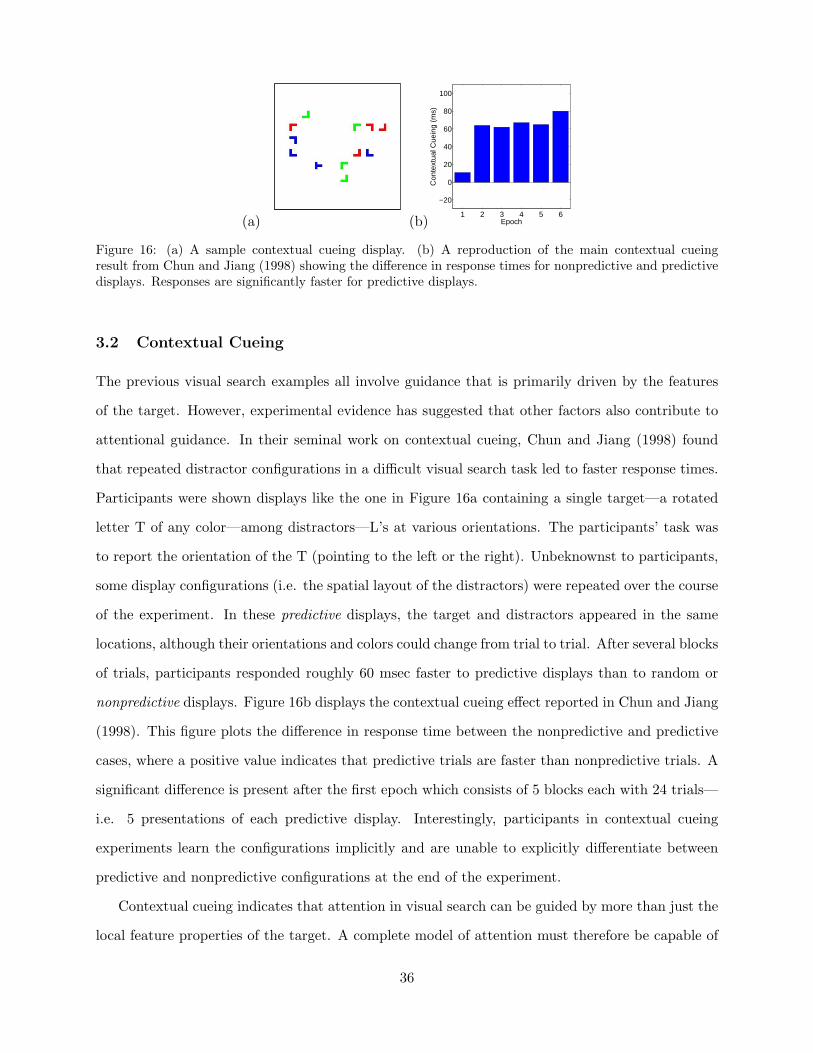
(a) (b)1 2 3 4 5 6

−20

0

20

40

60

80

100

Epoch

Con

text

ual C

uein

g (m

s)

Figure 16: (a) A sample contextual cueing display. (b) A reproduction of the main contextual cueingresult from Chun and Jiang (1998) showing the difference in response times for nonpredictive and predictivedisplays. Responses are significantly faster for predictive displays.

3.2 Contextual Cueing

The previous visual search examples all involve guidance that is primarily driven by the features

of the target. However, experimental evidence has suggested that other factors also contribute to

attentional guidance. In their seminal work on contextual cueing, Chun and Jiang (1998) found

that repeated distractor configurations in a difficult visual search task led to faster response times.

Participants were shown displays like the one in Figure 16a containing a single target—a rotated

letter T of any color—among distractors—L’s at various orientations. The participants’ task was

to report the orientation of the T (pointing to the left or the right). Unbeknownst to participants,

some display configurations (i.e. the spatial layout of the distractors) were repeated over the course

of the experiment. In these predictive displays, the target and distractors appeared in the same

locations, although their orientations and colors could change from trial to trial. After several blocks

of trials, participants responded roughly 60 msec faster to predictive displays than to random or

nonpredictive displays. Figure 16b displays the contextual cueing effect reported in Chun and Jiang

(1998). This figure plots the difference in response time between the nonpredictive and predictive

cases, where a positive value indicates that predictive trials are faster than nonpredictive trials. A

significant difference is present after the first epoch which consists of 5 blocks each with 24 trials—

i.e. 5 presentations of each predictive display. Interestingly, participants in contextual cueing

experiments learn the configurations implicitly and are unable to explicitly differentiate between

predictive and nonpredictive configurations at the end of the experiment.

Contextual cueing indicates that attention in visual search can be guided by more than just the

local feature properties of the target. A complete model of attention must therefore be capable of

36

exploiting image properties that extend beyond the target. Here we demonstrate that the TASC

model leverages predictive spatial configurations to boost saliency values in relevant locations. As

in the previous simulations, a row of modules is trained for a specific target, which in this case is a

sideways T. This training stage corresponds to the practice trials in a contextual cueing experiment.

The images in the training phase are standard contextual cueing displays except that none of the

configurations are predictive. As in Chun and Jiang (1998), the model is then presented with

30 blocks of 24 images, 12 with predictive displays that repeat from block to block and 12 with

nonpredictive displays that always change. The displays were generated using the same methods

as in Chun and Jiang (1998). Because the contextual cueing effect depends on the sequential

presentation of trials, the association component of each TASC module was modified to perform

online learning while displays are presented in order. This differs from the batch learning used for

other simulations. Two computations occur at each trial: a forward pass in the neural network

yields a saliency map for the current display (used for evaluation) and a backward pass updates

the weights to reflect the current trial. In this way the association components of each module

are constantly changing such that performance on future trials is affected by recent experience.

Sequential predictions are inherently noisier because they originate from an average over fewer

trials than predictions that are based on averages performed across the entire experiment. To

account for this, results were obtained from the average of 5 simulations. As in the previous visual

search experiments, the target ranking in the final combined saliency map is used as a measure of

response latency. Figure 17a shows the difference in ranking between nonpredictive and predictive

trials and exhibits a pattern very similar to Chun and Jiang’s behavioral result in Figure 16b. In this

figure, the 30 blocks of trials are grouped into 6 epochs each with 5 blocks. Most importantly, both

figures show no difference between the two cases at the onset of the experiment and a noticeable

difference beginning in the second epoch. Figure 17b depicts the block by block learning pattern

for predictive and nonpredictive displays. Learning occurs quickly for the predictive displays and

performance is greatly facilitated compared to the minimal improvement for nonpredictive displays.

Figure 17a can be obtained from Figure 17b by averaging across groups of 5 blocks and computing

the difference between cases.

The results presented in Figure 17 are obtained from the final saliency map that represents a

combination across all ranges of influence. But which ranges of influence are most responsible for

37

(a)1 2 3 4 5 6

0

1

2

3

Mea

n R

ank

Diff

eren

ce

Epoch (b)5 10 15 20 25 30

1

2

3

4

5

6

Block

Mea

n Sa

lienc

y R

ank

PredictiveNonpredictive

Figure 17: (a) Contextual cueing simulation results showing the difference in rank between the nonpredictiveand predictive displays. Predictive ranks are significantly lower after the first epoch. (b) Block by blockresults showing the mean rank for predictive and nonpredictive displays.

Short Long

1

2

3

4

5

Range of Influence

Mea

n R

ank

PredictiveNonpredictive

Figure 18: Mean ranks for the 4 ranges of influence in TASC from the contextual cueing simulation. Thefirst 5 blocks are removed from the averages. The two longest ranges of influence demonstrate significantfacilitation for displays with predictive contexts.

38

producing the contextual cueing effect? Intuition implicates longer ranges of influence because short

ranges cannot detect configurations of distractors that extend beyond a local region. Support for

this intuition can be found by examining the saliency maps for each range of influence separately.

Figure 18 presents the average predictive and nonpredictive rank across the whole simulation for

the 4 ranges of influence. The first 5 blocks are removed from each average because significant

learning occurs during those trials. It is clear that the difference in rank increases as the range

of influence grows and that the target rank for predictive displays decreases with longer ranges of

influences. The two longest ranges of influence appear to be responsible for most of the response

time facilitation.

In the context of the TASC control space, contextual cueing, with its dependence on the long

ranges of influence, corresponds to an attentional strategy that primarily exploits the region of

the control space with high task specificity and a global spatial scale. A natural comparison can

be drawn between contextual cueing and scene-based endogenous control; in both cases, attention

is guided by coarse properties of the image. Similarly, a parallel can be made between distrac-

tor configurations and scene gists. However, TASC predicts that contextual cueing is not just a

consequence of the global spatial scale. As suggested by Figure 18, the second longest range of

influence—which covers quadrants of the image—is also capable of producing the effect. This dif-

ference between contextual cueing and scene-based endogenous control suggests another strategy

that can be placed in the TASC control space. Figure 19 adds a point for contextual cueing to

the control space that has relatively high task specificity and an intermediate spatial scale near

the global end of the spectrum. Contextual cueing is placed lower than scene-based endogenous

control on the task specificity axis because the same configuration could provide facilitation for a

variety of target objects. Thus the relationship between a specific target and the contextual cueing

configuration is weaker than the relationship between an object and the scene gist in a real-world

task. In essence, contextual cueing could still have an effect when the task is more loosely de-

fined. The prediction in TASC that contextual cueing draws from an intermediate spatial scale

is supported by a subsequent contextual cueing experiment that observed the contextual cueing

effect even when predictive configurations were constrained to one quadrant of the image (Olson

and Chun, 2002). Additionally, no response time facilitation was found in this experiment when

configurations distant to the target were repeated and local configurations were novel.

39

feature-basedendogenous

exogenous

scene-basedendogenous

Spatial ScaleTa

sk S

peci

ficity

local global

low

high

contextual cueing

lower region

Figure 19: The control space depiction with two points added for contextual cueing and the lower regioneffect. The experimental results from these two paradigms suggest that individuals employ control strategieslocated in different regions of the control space than the primary strategies.

Recent research on contextual cueing with real-world displays has led to alternative conclusions

about how global and local contexts affect response times (e.g., Brockmole et al., 2006). Contrary

to the result of Olson and Chun (2002), this research concludes that observers use global contex-

tual cues for attentional guidance far more than local contextual cues. Using simulated real-world

scenes, the authors manipulated objects in the local region of the target and the objects surrounding

that local region which form the global context. As expected, the greatest response time facilita-

tion occured when the local and global context were both predictive. However, when predictive

local contexts were compared to predictive global contexts, local contexts provided significantly less

facilitation than global contexts. The conflict between these results and those in Olson and Chun

seems to stem from the inherent difference between artificial displays and real-world scenes. The

TASC framework offers a potential resolution to this conflict by allowing for the possibility that

attentional emphasis is placed on different regions of the control space for these two experiments.

The global spatial scale could be of high importance for real-world scenes whereas intermediate

spatial scales might be preferred for less familiar images that lack an understandable global struc-

ture. This viewpoint fits with the concept that modules are used according to their relevance to

the current goals and environment. Experience may build an attentional bias for the global spatial

scale when the viewing environment consists of real-world scenes. This conclusion requires more

rigorous support, however, the notion that contextual guidance is tuned through experience to real-

world environments is partially bolstered by the findings in Brockmole et al. (2006) that predictive

40

configurations in real-world scenes are learned more quickly and ultimately lead to a greater re-

sponse time facilitation than predictive configurations in artificial search images. Experience with

the contextual properties of real-world scenes evidently results in a greater impact on attentional

guidance. We expect that TASC would produce results consistent with those in Brockmole et al.

(2006) if ranges of influence were selectively chosen based on the visual environment and the goals

of the task.

3.3 Spatial Probability Cues

To assure that distractor configurations are responsible for the effect found in contextual cueing

experiments, the arrangement of displays is controlled such that predictive target locations are

equally as probable as nonpredictive target locations. Motivation for this constraint comes from

findings in Geng and Behrmann (2005) that suggest that spatial probability is another factor that

influences attentional guidance. The authors report response latencies that are faster for targets

in locations that frequently contain a target compared to locations were targets rarely appear.

The implementation of TASC allows the model to naturally exploit spatial probability cues of this

sort when forming saliency predictions. Specifically, the neural networks of each module indirectly

encode the prior probability of a target appearing at each location within their scope (i.e. if a

specific location is frequently active, it will generally yield higher activations than infrequently

active locations). If the same target features appear in separate images at two different locations—

one with high probability and one with low probability—the networks will yield higher activation

for the target at the highly probable location and consequently the target-distractor saliency ratio

will be greater for that target and the response time faster.

Geng and Behrmann also find that response times associated with targets in low probability

locations are slower when a distractor appears in a highly probable location as opposed to when

the highly probable locations are empty. TASC would also produce this effect because the module

networks have weak discrimination abilities. If a network regularly gives a response to a high

probability region, then a distractor in that location would likely produce more activity than if it

were in a low probability location, thus hindering the ranking of the actual target.

The spatial probability cues in Geng and Behrmann are are learned over a relatively short

time frame (within one group of trials). In contrast, spatial probability cues in Senders (1964) are

41

learned over the span of days and weeks. TASC is capable of learning at both of these time scales.

If modified to process trials sequentially, as in the contextual cueing simulation, the association

networks would show a short term preference for locations that more recently contained targets.

Additionally, if networks were exposed to regular patterns of information over a longer period of

time, the model would acquire a bias for frequently relevant locations. This behavior is a direct

consequence of the claim embedded in TASC that attention is fundamentally experience-based and

we elaborate on this point in the discussion.

3.4 Figure-ground Assignment

Expanding upon the long term learning of spatial probability cues, one might expect a spatial bias

for locations found to be important based on a lifetime of experience. Vecera et al. (2002) find

evidence for such a bias in what they refer to as the lower-region effect in figure-ground assignment.

The authors observed that for displays such as the blocky images in Figure 20, viewers tended to

perceive the lower region as the foreground figure regardless of the arrangement of colors. This

result can be interpreted as an attentional bias for the lower region—i.e. people attend the lower

region first and thus consider it the foreground figure. An intuitive explanation for this effect can

be drawn from the observation that in real-world situations, objects of interest are more often found

in the lower region of our field of view (things are on the ground more often than they are in the

sky).

The TASC framework offers an informative interpretation of the lower-region effect. Specifically,

this effect can be viewed as exogenous control that operates at a global spatial scale and has low

task specificity—i.e., it is based on the overall scene properties and requires no specific target of

search. This strategy is markedly different from scene-based endogenous control in that it operates

with low task specificity. We have indicated this new point in the control space in Figure 19. Lower

region, occupying the fourth corner of the control space, is a natural complement to the three

primary control strategies described previously. To demonstrate that TASC obtains the lower-

region effect, an instantiation with 11 object module rows was trained on a corpus of real-world

images using the following objects: car, person, tree, window, bike, light, building, sidewalk, road,

head, and sign. The model was then exposed to displays (shown in Figure 20) similar to those in

Vecera et al. (2002) with noise added to increase the amount of feature information in the lower

42

Figure 20: Sample displays from Vecera et al. (2002) and the associated outputs from TASC operating atthe longest range of influence and with low task specificity, combining across 11 object models trained onreal-world images. A bias is shown for the lower region in both displays.

and upper regions. The saliency maps in Figure 20 are a combination across all object modules

using only the longest range of influence. Because the displays bear no resemblance to real-world

images, the activity patterns in the saliency maps are difficult to interpret. However, TASC does

show a clear bias for attending the lower region of the image regardless of the color layout—i.e.

there is more saliency activity in the bottom half of both maps. These saliency maps are obtained

from a limited instantiation of TASC with only 11 objects and thus one can justifiably be cautious

in making strong claims about this result. Nevertheless, the result is an emergent consequence of

training TASC solely on real-world scenes.

Throughout this paper, the term exogenous control has been used to refer to bottom-up atten-

tional processing at a local spatial scale. This usage is consistent with most of the literature on

attention. In the lower-region effect, however, we recognize a different form of exogenous behavior

that operates at a global spatial scale. From the perspective of the TASC framework, exogenous

attention—defined to be any attention that is driven primarily by factors outside the individual—

should correspond to the entire bottom region in the control space—i.e. low task specificity across

all spatial scales. This new conceptualization of exogenous attention may prove useful in evalu-

ating attentional behavior in unstructured viewing situations. We embrace this new perspective;

however, throughout the rest of the paper, we continue to use the term exogenous control with its

traditional meaning.

3.5 Real-world Images

The simulations in the previous sections demonstrate that TASC yields results consistent with the

findings in a variety of attentional experiments with artificial images. This consistency provides

a strong argument for the theory behind TASC. However, any complete model of visual attention

43

must also be tested on real-world images; after all, the ultimate goal of this inquiry is to understand

how people allocate attention in real-life situations.

In much of the attention literature, results for real-world images lack quantitative analysis

offering instead only weak qualitative assessments. Torralba et al. (2006) provide a more rigorous

analysis in which saliency predictions from the TOCH model are compared directly to human eye-

movements recorded for the same set of images. The experiment in Torralba et al. (2006) involved

three different search tasks over a set of images that contained indoor and outdoor scenes. For

each target object—person, mug, and painting—an ordered sequence of fixation locations for each

image was collected from 8 participants. Saliency maps for each image were also obtained from

a version of TOCH tuned to the relevant target object. The model’s performance for each image

was measured by computing the percent of participant fixations within the most active regions of

the saliency map. These highly active regions contain all locations with a saliency value among

the top 20 percent of values and thus cover 20 percent of the image’s area. The saliency maps

of TOCH were compared to saliency maps representing cross-participant consistency and saliency

maps obtained from a simple bottom-up model similar to model of Itti and Koch (2000). For

each image and participant, the cross-participant saliency map was constructed using a mixture of

Gaussians, one for every fixation location of every participant except the current participant. Cross-

participant consistency was then measured by computing the percent of the current participant’s

fixations located within the most active regions in this constructed saliency map. Cross-participant

consistency proved to be high and thus provided a useful upper limit for model comparison.

To assess TASC’s performance on real-world images, we tested the model on the same set of

images used by Torralba et al. (2006). Other state of the art models (e.g. Kanan et al., 2009)

have reported similar or better performance than TOCH on this dataset, but for simplicity, we

assess TASC’s performance in the context of the results presented in Torralba et al. (2006). A

TASC instantiation with 3 object module rows, was trained on the image corpus with the set of

test images removed. Saliency maps were generated from the object module row relevant to the

specific task and performance was measured using the method described above. Figure 21 presents

the performance of TASC alongside results reproduced from Torralba et al. (2006). The results are

divided by target object and by whether the target was present or absent. Each bar graph is further

divided along the abscissa by fixation number. Thus the light blue bar corresponding to fixation 1

44

in the upper left graph expresses that for the person search task with target present images, on

average about 65% of the participants’ first fixation in an image fell within the top 20 percent

of the TASC saliency map for that image. Across all search cases and fixation numbers, TASC’s

performance is on average between the TOCH model and the simple bottom-up model (BU). It is

important to note that the TASC instantiation used here was not optimized for these images and

search tasks. Instead, the model parameters were carried over from the visual search simulations

with artificial images. Because characteristics of real-world images are quite different than those

of artificial search images, it seems likely that image processing parameters selected for synthetic

images would be sub-optimal for real-world images—e.g. the sizes used for the center and surround

regions in the contrast enhancement stage. Additionally, performance is limited in this simulation

by the naive assumption that for a given task, all ranges of influence are equally relevant. This

latter assumption is likely responsible for TASC’s relatively poor performance in the mug search.

This relationship can be understood by noting that the performance of the BU model is closest to

TOCH in mug search. Because TOCH consists of a bottom-up model filtered by global contextual

guidance, the similarity between TOCH and BU in this task suggests that mug locations are only

weakly predicted by global scene properties. Hence, the bottom-up component of TOCH, which

operates on local feature information, is responsible for most of the model’s predictive power. In

the naive version of TASC, however, all ranges of influence are combined equally thus causing a

dilution of the shortest range of influence by the longer ranges. In fact, the saliency maps obtained

from the shortest range of influence alone perform similarly to TOCH and BU in the mug search

task. Despite these limiting factors, the present result demonstrates that TASC’s performance for

real-world images is similar to other major models.

The results for the first three fixations in Figure 21 are obtained using the same saliency map.

But is there any relationship between successive fixations that might motivate the use of a different

saliency map for each fixation? Analysis of the eye-movement data in Torralba et al. (2006) reveals

that participants tend to saccade to locations in close proximity to the previous fixation location. Of

course some fixations select a completely new region, but these are less common. This observation

conflicts with the standard inhibition of return explanation used to generate fixation sequences in

other attentional models including Itti and Koch (2000). The predictive quality of the last fixation

can be assessed by building a saliency map with a Gaussian centered around the last fixation

45

1 2 340

60

80

100Person Present

1 2 340

60

80

100Person Absent

HumanTASCTOCHBU

1 2 340

60

80

100Mug Present

Perc

ent o

f Fix

atio

ns in

Thr

esho

lded

Reg

ion

(20%

)

1 2 340

60

80

100Mug Absent

1 2 340

60

80

100Painting Present

Fixation Number1 2 3

40

60

80

100Painting Absent

Fixation Number

Figure 21: TASC performance on the eye-movement dataset used in Torralba et al. (2006). TASC is placedalongside TOCH, a bottom-up model (BU), and cross-participant consistency. The measure is percent ofhuman eye-movements contained in the top 20% of the saliency map. The data is divided into the first threefixations.

46

1 2 330

40

50

60

70

80

90

100

Fixation NumberPe

rcen

t of F

ixat

ions

TASC with last fixationTASCJust last fixationTOCH

Figure 22: A model predicting the current fixation location based on the last fixation location performscomparably to major attention models. TASC shows an improvement when previous fixation information isincluded suggesting that both models contain valuable information. The results here represent an averageover the 3 tasks and target present/absent cases in the previous figure.

location. Performance for the current fixation can be measured by thresholding this last fixation

map in the same manner described above. The magenta bars in Figure 22 display the percent of

fixations that are in close proximity to the previous fixation—i.e. the percent of fixations that fall

within a circle covering 20 percent of the image and centered around the last fixation location.

For the first fixation, the saliency map is constructed using one centrally located Gaussian. The

results presented here represent an average across the three tasks and the present/absent cases.

Interestingly, the previous fixation alone proves to be as good a predictor of the current fixation

as other attentional models including TASC and TOCH. The figure also shows that performance

is improved when the TASC saliency map is averaged with the last fixation map, suggesting that

both elements provide distinctly useful information for predicting attentional shifts.

The relationship between successive fixation locations is consistent with any model that encodes

the effort required to change the locus of attention, where shorter saccades are preferred because

they require less effort. The SEEV model proposed by Wickens (2007) explicitly incorporates this

effort component. SEEV is a utility based framework that combines task independent influences

with knowledge driven components. Specifically, SEEV models the probability of attending a

location as a linear combination of four factors: Salience, Effort, Expectancy, and Value. The

salience component corresponds to bottom-up attention as defined in models such as Itti and Koch

(2000). Effort represents the cost of attending a new location—i.e. the physical cost of moving

the eyes, head, or whole body—and has a negative influence on saliency. Expectancy is a top-

47

down component that represents the likelihood that a specific region contains information. The

value component models the importance of attending a specific region based on the gains (losses)

associated with fixating (not fixating) that region. As in TASC, experience plays a fundamental

role in tuning the expectancy and value components of SEEV. A utility based theory such as SEEV

is compatible with the TASC framework and the combination of the two would result in a more

powerful model that could capture results such as the relationship between subsequent fixations.

4 Discussion

We have introduced a unified framework for addressing a broad range of phenomena pertaining

to attentional control. This framework, instantiated in the TASC model, describes human visual

search in both naturalistic scenes and in artificial displays consisting of simple elements varying

in color and shape. Our goal in this work was to develop TASC to the point that it serves as an

existence proof of an attention theory that is based fundamentally on the role of experience, a theory

that makes contact with diverse phenomena and can serve an an integrative framework. TASC

borrows from many other theories of attention, and in so doing, it serves as a synthesis of existing

theories and as a means of characterizing the relationships among the theories. TASC follows a clear

trend in the literature toward models that are comprehensive in scope and incorporate multiple

attentional control strategies (e.g., Kanan et al., 2009; Navalpakkam and Itti, 2005; Torralba et al.,

2006; Zhang et al., 2008). TASC is perhaps distinguished by the fact that the distinct control

strategies in TASC are implemented by the same underlying mechanisms. Through simulations,

we showed that exogenous control, feature-based endogenous control, and scene-based endogenous

control could all emerge from the same underlying processing machinery.

Embedded in the TASC framework is a key proposition: attentional control is fundamentally

experience based. TASC consists of a collection of modules, each of which is specialized to the

detection of a particular entity, and is assumed to arise from experience with the world, and to

continually adapt to the ongoing stream of experience. These entities can be what are traditionally

referred to as features, such as the color red, or simple shapes, such as a square, or complex,

hierarchical, articulated objects, such as a person. We’ve loosely referred to these entities as

objects, although this usage stretches the canonical notion of objects in vision. The important

48

point is that these objects are functionally defined—they are the goals of visual search, goals that

have been rewarded and learned in the past.

According to TASC, attentional control varies in the degree of task (object) specificity via the

combination of object modules. By this conception, what is typically considered top-down control

occurs when one or a small number of object modules contribute to saliency; and what is typically

considered bottom-up control occurs when all object modules contribute to saliency. Instead of

considering exogenous control as a search with no target in mind, TASC conceptualizes it as a

search for all possible objects. Consequently, TASC rejects the notion of pure bottom-up saliency,

instead favoring the hypothesis that control always operates in a top-down manner, tuned through

experience.

Failure of attentional control to exclude task irrelevant signals can be attributed to limitations

on the degree of task specificity that can be achieved. On grounds of survival, it may be adaptive for

an organism not to become so focused on the task at hand that all extraneous warning signals from

the environment are suppressed. As a result, we suppose that critical object modules contribute to

saliency even when not pertinent to current goals. For example, the presence of a human face may

be important to many different goals, including basic survival in a community. Thus, attentional

capture can be considered not as a failure of attentional control to stay on task, but as the inability

of attentional control to narrow to a single task.

4.1 The role of experience

Many recent theories of attention have begun to focus on the role of experience in attentional

control. TASC is motivated in part by TOCH, whose contextual component, presented in Torralba

(2001, 2003), encodes and exploits correlations between scene gist and the locations of specific

objects. Rao et al. (2002) also implement a model for visual search in which saliency is based on

how well local visual features match a specific object template. Similarly, the SAIM model of Heinke

and Humphreys (1997, 2003) incorporates object templates to determine a focus of attention via

constraint-satisfaction dynamics.

These previous theories assume that experience leads to the learning of specific object models.

Recent Bayesian theories instead assume that experience results in learning of statistical properties

of the environment, which might steer attention to locations containing surprising visual informa-

49

tion, or might optimize attention to situations that are likely to occur in the future. While the

various Bayesian theories agree in claiming that attention is modulated by statistics of the envi-

ronment, they differ in terms of the time period over which statistics are collected. Some theories

rely on life long history (e.g., Kanan et al., 2009; Torralba, 2003; Zhang et al., 2008), some theories

rely on the recent history of experience, and suggest trial-to-trial modulations of attention (e.g.,

Itti and Baldi, 2009; Mozer and Baldwin, 2008; Mozer et al., 2006; Yu and Dayan, 2005), and

finally, some theories assume that experience doesn’t extend beyond the statistics of the current

image (e.g. Bruce and Tsotsos, 2009; Torralba et al., 2006, bottom-up component). Like all of these

theories, TASC can be cast in a probabilistic framework, as described in an earlier section of the

paper. TASC has the virtue of spanning a range of time scales of adaptation. Some simulations

we presented rely on experience on the time scale of years (e.g., attention in real-world scenes,

lower region bias in figure-ground assignment); other simulations rely on experience on the time

scale of minutes (e.g., contextual cueing). Regardless of how TASC plays out compared to other

probabilistic theories, we view TASC as the culmination of a shift in the field, from the assumption

of hardwired, fixed mechanisms of attention to the view that every aspect of attentional control

relies on adaptation to the ongoing stream of experience.

4.2 Adaptation of attentional control

Up to this point we’ve used TASC to explain adaptation in a way focussed on how object modules

arise from experience—i.e. how the neural nets change the associative weights to encode experience.

However, TASC suggests a complementary sort of adaptation that we haven’t discussed which

occurs when the set of modules relevant to a particular goal change. The TASC architecture

assumes that for a specific goal, saliency predictions are obtained by taking a disjunction across

a subset of modules that correspond to the objects and ranges of influence related to the goal.

The predictions obtained by TASC are thus dependent on the particular subset of modules. In the

simulations presented in this work, the subset of modules relevant to a particular search experiment

were selected in advance and remained fixed throughout the simulation. If instead this subset

were to change throughout the course of an experiment, attentional behavior would also change.

Modification of the set of relevant modules could serve as a form of adaptation of attentional control.

A natural extension to the approach in the current implementation, which gives all selected modules

50

equal weight, is to combine across all modules giving each one a weight based on its relevance to

the goal. Under this approach, adaptation would occur if the module weights associated with each

goal were constantly revised to reflect experience.

4.3 The relation of attention and object recognition

Under the conceptualization of saliency proposed by TASC, the goal of attention is to identify

locations in the image containing objects of interest. So what distinguishes TASC from full-blown

object recognition models? The primary difference is that TASC is computationally limited by

the dimensionality reduction stage and the restrictions placed on the neural nets. Another point

that sets TASC apart from most object recognition models is that processing occurs in parallel

across the entire visual field without any recurrent loops. These differences are important because

computational simplicity and efficiency should go hand-in-hand with speed in the brain, and a quick

response is essential if saliency is to provide useful guidance for more detailed, computationally

intensive object recognition and scene interpretation processes.

In object recognition models, it is common to exploit as much of the feature data as possible,

even in the face of significant additional computational requirements. In essence, TASC employs a

contrasting strategy: discard as much feature data as possible while still preserving at least some

of the predictive qualities. Extraneous feature data is removed in the sub-sampling and principal

components analysis (PCA) stages of processing. PCA is often used by object recognition models to

organize the feature data in a more compact form without losing its expressive power. The difference

between PCA in TASC and other object recognition models is the number of principal components

preserved. Whereas object recognition models typically keep enough principal components such

that little is lost from the original data, TASC uses only a few principal components, thus extracting

just the primary trends of the data. The choice between different levels of dimensionality reduction

ultimately results in a trade off between efficiency and precision of predictions. The design of

TASC is based on the assumption that attention sacrifices some precision in order to provide faster

guidance.

The linearity of the associative neural nets in TASC also limits the model’s computational

complexity. The output of each network is obtained via a rank-limited linear mapping of the di-

mensionality reduced feature data, implemented using a hidden layer with few units. The mapping

51

of the input units onto the hidden units can be viewed as an additional dimensionality reduction

step. The difference between this reduction and the PCA reduction is that the mapping is cus-

tomized for each object—i.e. PCA selects features that are generally informative across all images

whereas this mapping selects features that are important for a specific object. The features encoded

by the hidden units are then combined linearly to generate output activations. The linearity of the

system is broken when the output values are scaled by the sigmoid function. However, because the

sigmoid function is monotonic, the relative ranking of output units is preserved.

Through this one-pass feedforward processing stream, the TASC modules estimate the proba-

bility that a specific object is present at each location given the surrounding visual features. These

estimates are computed quickly at the expense of high levels of precision, thus providing a coarse

form of object recognition or detection. This key property of the TASC theory implies that the

attentional system, in its essence, always performs a crude sort of object recognition, even when

the viewing goals do not involve specific objects. Objects are coarsely recognized from local feature

properties, global scene properties, and intermediate regional feature properties. Predictions from

these rudimentary object detection components are brought together to yield saliency predictions

customized for specific viewing situations. The details of these object components, the combina-

tion rules across them, and even the object definitions themselves are all constantly tuned through

experience to yield an adaptive attentional system capable of providing useful guidance across a

wide range of search goals and visual environments.

5 Acknowledgments

This research was supported by NSF BCS 0339103, NSF CSE-SMA 0509521, and NSF BCS-

0720375.

References

E. Averbach and A. Coriell. Short-term memory in vision. Bell Systems Technical Journal, 40:309–328, 1961.

W. Bacon and H. Egeth. Overriding stimulus-driven attentional capture. Perception and Psy-chophysics, 55:485–496, 1994.

I. Biederman. Perceiving real-world scenes. Science, 177:77–80, 1972.

52

J. Brockmole, M. Castelhano, and J. Henderson. Contextual cueing in naturalistic scenes: Globaland local contexts. Journal of Experimental Psychology: Learning, Memory, and Cognition, 32:699–706, 2006.

J. Brockmole, D. Hambrick, D. Windisch, and J. Henderson. The role of meaning in contextualcueing: Evidence from chess expertise. Quarterly Journal of Experimental Psychology, 2008.

N. Bruce and J. Tsotsos. Saliency, attention, and visual search: An information theoretic approach.Journal of Vision, 9(3):5, 1–24, 2009.

M. Cerf, E.P. Frady, and C. Koch. Using semantic content as cues for better scanpath prediction.Proceedings of the symposium on Eye tracking research & applications, pages 143–146, 2008a.

Moran Cerf, Jonathan Harel, Wolfgang Einhaeuser, and Christof Koch. Predicting human gazeusing low-level saliency combined with face detection. In J.C. Platt, D. Koller, Y. Singer, andS. Roweis, editors, Advances in Neural Information Processing Systems 20. MIT Press, Cam-bridge, MA, 2008b.

M. Chun and Y. Jiang. Contextual cueing: Implicit learning and memory of visual context guidesspatial attention. Cognitive Psychology, 36:28–71, 1998.

C. Folk, R. Remington, and J. Johnston. Involuntary covert orienting is contingent on attentionalcontrol settings. Journal of Experimental Psychology: Human Perception and Performance, 18:1030–1044, 1992.

D. Gao, V. Mahadevan, and N. Vasconcelos. On the plausibility of the discriminant center-surroundhypothesis for visual saliency. Journal of Vision, 8(7):13, 1–18, 2008.

T. Gawne and J. Martin. Responses of primate visual cortical v4 neurons to simultaneously pre-sented stimuli. Journal of Neurophysiology, 88:1128–1135, 2002.

J. Geng and M. Behrmann. Spatial probability as an attentional cue in visual search. Perception& Psychophysics, 67(7):1252–1268, 2005.

D. Heinke and G. Humphreys. Saim: A model of visual attention and neglect. In InternationalConference on Artificial Neural Networks, pages 913–918, 1997.

D. Heinke and G. Humphreys. Attention, spatial representation and visual neglect: Simulatingemergent attention and spatial memory in the selective attention for identification model (SAIM).Psychological Review, 110:29–87, 2003.

L. Itti and P. Baldi. Bayesian surprise attracts human attention. Vision Research, 49(10):1295–1306, 2009.

L. Itti and C. Koch. A saliency-based search mechanism for overt and covert shifts of visualattention. Vision Research, 40(10-12):1489–1506, May 2000.

L. Itti, C. Koch, and E. Neiber. A model of saliency-based visual attention for rapid scene analysis.IEEE Transactions on Pattern Analysis and Machine Intelligence, 20(11):1254–1259, 1998.

B. Julesz. Toward an automatic theory of preattentive vision. In G. M. Edelman, W. E. Gall, andW. M. Cownan, editors, Dynamic aspects of neocortical function, pages 595–612. NeurosciencesResearch Foundation, New York, 1984.

53

C. Kanan, M. Tong, L. Zhang, and G. Cottrell. Sun: Top-down saliency using natural statistics.Visual Cognition, 17(6-7):979–1003, 2009.

C. Koch and S. Ullman. Shifts in selective visual attention: Towards the underlying neuronalcircuitry. Human Neurobiology, 4:219–227, 1985.

I. Lampl, D. Ferster, T. Poggio, and M. Riesenhuber. Intracellular measurements of spatial inte-gration and the MAX operation in complex cells of the cat primary visual cortex. Journal ofNeurophysiology, 92:2704–2713, 2004.

D. Lamy, T. Carmel, H. Egeth, and A. Leber. Effects of search mode and intertrial priming onsingleton search. Perception and Psychophysics, 68:919–932, 2006.

M. Mozer. The perception of multiple objects: A connectionist approach. MIT Press, Cambridge,MA, 1991.

M. Mozer and D. Baldwin. Experience-guided search: A theory of attentional control. In J. Platt,D. Koller, and Y. Singer, editors, Advances in Neural Information Processing Systems 20. MITPress, Cambridge, MA, 2008.

M. Mozer, M. Shettel, and S. Vecera. Control of visual attention: A rational account. In Y. Weiss,B. Schoelkopf, and J. Plattr, editors, Neural Information Processing Systems 18, pages 923–930.MIT Press, Cambridge, MA, 2006.

V. Navalpakkam and L. Itti. Modeling the influence of task on attention. Vision Research, 45:205–231, 2005.

M. Neider and G. Zelinsky. Scene context guides eye movements during visual search. VisionResearch, 46:614–621, 2006.

U. Neisser. Cognitive psychology. Appleton-Century-Crofts, New York, 1967.

A. Oliva and A. Torralba. Modeling the shape of the scene: a holistic representation of the spatialenvelope. International Journal of Computer Vision, 42(3):145–175, 2001.

I. Olson and M. Chun. Perceptual constraints on implicit learning of spatial context. VisualCognition, 9:273–302, 2002.

M. Peterson and E. Skow-Grant. Memory and learning in figure-ground perception. In B. Ross andD. Irwin, editors, Cognitive Vision: Psychology of Learning and Motivation, volume 42, pages1–34. 2004.

M. Posner and Y. Cohen. Components of visual orienting. In H. Bouma and D. G. Bouwhuis,editors, Attention and Performance X, pages 531–556. Erlbaum, Hillsdale, NJ, 1984.

Rajesh P Rao, Gregory J Zelinsky, Mary M Hayhoe, and Dana H Ballard. Eye movements in iconicvisual search. Vision Research, 42(11):1447–1463, 2002.

M. Riesenhuber and T. Poggio. Hierarchical models of object recognition in cortex. Nature Neuro-science, 2:1019–1025, 1999.

B. Russel, A. Torralba, and K. Murphy. Labelme: a database and web-based tool for imageannotation. International Journal of Computer Vision, 77(1-3):157–173, May 2008.

54

J. Senders. The human operator as a montior and controlller of mulitdegree of freedom systems.IEEE Transactions on Human Factors in Electronics, 5:2–6, 1964.

C. Siagian and L. Itti. Rapid biologically-inspired scene classification using features shared withvisual attention. IEEE Transactions on Pattern Analysis and Machine Intelligence, 29(2):300–312, 2007.

E. Simoncelli and W. Freeman. The steerable pyramid: a flexible architecture for multi-scalederivative computation. In 2nd Annual Intl. Conf. on Image Processing, 1995.

A. Torralba. Contextual modulation of target saliency. Adv. in Neural Information ProcessingSystems, 14:1303–1310, 2001.

A. Torralba. Modeling global scene factors in attention. Journal of Optical Society of America, 20(7):1407–1418, 2003.

A. Torralba, A. Oliva, M. Castelhano, and J. Henderson. Contextual guidance of eye movementsand attention in real-world scenes: The role of global features on object search. PsychologicalReview, 113(4):766–786, October 2006.

A. Treisman. Perceptual grouping and attention in visual search for features and objects. Journalof Experimental Psychology: Human Perception and Performance, 8:194–214, 1982.

A. Treisman and G. Gelade. A feature-integration theory of attention. Cognitive Psychology, 12:97–136, 1980.

S. Vecera, E. Vogel, and G. Woodman. Lower region: A new cue for figure-ground assignment.Journal of Experimental Psychology: General, 131:194–205, 2002.

C. Wickens. Attention to attention and its applications: A concluding view. In A. Kramer,D. Wiegmann, and A. Kirlik, editors, Attention: From Theory to Practice. Oxford UniversityPress, New York, 2007.

J. Wolfe. Guided search 2.0: A revised model of visual search. Psychonomic Bulletin and Review,1:202–238, 1994.

J. Wolfe. Visual memory: What do you know about what you saw? Current Biology, 8:R303–R304,1998a.

J. Wolfe. What can 1,000,000 trials tell us about visual search? Psychological Science, 9(1):33–39,1998b.

J. Wolfe. Guided search 4.0: Current progress with a model of visual search. In W. Gray, editor,Integrated Models of Cognitive Systems, pages 99–119. Oxford, New York, 2007.

J. Wolfe and T. Horowitz. What attributes guide the deployment of visual attention and how dothey do it? Nature Reviews Neuroscience, 5:1–7, 2004.

J. Wolfe, K. Cave, and S. Franzel. Guided search: An alternative to the feature integration modelfor visual search. Journal of Experimental Psychology: Human Perception and Performance, 15:419–433, 1989.

A. Yu and P. Dayan. Inference, attention, and decision in a bayesian neural architecture. InAdvances in Neural Information Processing Systems, volume 17, pages 1577–1584, 2005.

55

L. Zhang, M. Tong, T. Marks, H. Shan, and G. Cottrell. Sun: A bayesian framework for saliencyusing natural statistics. Journal of Vision, 8(7):32, 1–20, 2008.

L. Zhaoping and R. Snowden. A theory of a saliency map in primary visual cortex (V1) tested bypsychophysics of colour-orientation interference in texture segmentation. Visual Cognition, 14:911–933, 2006.

56