A trajectory piecewise-linear approach to model order ... Trajectory Piecewise-Linear Approach to Model Order Reduction and Fast Simulation of Nonlinear Circuits and Micromachined

IEEE TRANSACTIONS ON COMPUTER-AIDED DESIGN OF INTEGRATED CIRCUITS AND SYSTEMS, VOL. 22, NO. 2, FEBRUARY 2003 155

A Trajectory Piecewise-Linear Approach to ModelOrder Reduction and Fast Simulation of Nonlinear

Circuits and Micromachined DevicesMichał Rewienski and Jacob White, Associate Member, IEEE

Abstract—In this paper, we present an approach to nonlinearmodel reduction based on representing a nonlinear system witha piecewise-linear system and then reducing each of the pieceswith a Krylov projection. However, rather than approximatingthe individual components as piecewise linear and then composinghundreds of components to make a system with exponentiallymany different linear regions, we instead generate a small set oflinearizations about the state trajectory which is the responseto a “training input.” Computational results and performancedata are presented for an example of a micromachined switchand selected nonlinear circuits. These examples demonstratethat the macromodels obtained with the proposed reductionalgorithm are significantly more accurate than models obtainedwith linear or recently developed quadratic reduction techniques.Also, we propose a procedure fora posteriori estimation of thesimulation error, which may be used to determine the accuracy ofthe extracted trajectory piecewise-linear reduced-order models.Finally, it is shown that the proposed model order reductiontechnique is computationally inexpensive, and that the models canbe constructed “on the fly,” to accelerate simulation of the systemresponse.

Index Terms—Microelectromechanical systems (MEMS), modelorder reduction, nonlinear analog circuits, nonlinear dynamicalsystems, piecewise-linear models.

I. INTRODUCTION

I NTEGRATED circuit fabrication facilities are now offeringdigital system designers the ability to integrate analog

circuitry and micromachined devices, but such mixed-tech-nology microsystems are extremely difficult to design becauseof the limited verification and optimization tools available.In particular, there are no generally effective techniques forautomatically generating reduced-order system-level modelsfrom detailed simulation of the analog and micromachinedblocks. Research over the past decade on automatic modelreduction has led to enormous progress in strategies for linearproblems, such as the electrical problems associated withinterconnect and packaging, but these techniques have beendifficult to extend to the nonlinear problems associated withanalog circuits and micromachined devices.

Manuscript received May 31, 2002; revised September 3, 2002. This workwas supported in part by the Defense Advanced Research Projects AgencyNeocad program, the National Science Foundation, and by grants from theSingapore-MIT Alliance. This paper was recommended by Guest Editor G.Gielen.

The authors are with the Department of Electrical Engineering and ComputerScience, Massachusetts Institute of Technology, Cambridge, MA 02139 USA(e-mail: [email protected]; [email protected]).

Digital Object Identifier 10.1109/TCAD.2002.806601

In this paper, we present an approach to nonlinear model re-duction based on representing a nonlinear system with a piece-wise-linear system and then reducing each of the pieces withKrylov subspace projection methods. However, rather than ap-proximating the individual components as piecewise-linear andthen composing hundreds of components to make a system withexponentially many different linear regions, we instead generatea small set of linearizations about the state trajectory which isthe response to a “training input.” At first glance, such an ap-proach would seem to work only when all the inputs are veryclose to the training input, but as examples will show, this is notthe case. In fact, the method easily outperforms recently devel-oped techniques based on quadratic reduction.

We start in the next section by describing examples of non-linear circuits and a micromachined switch, to make clear thenonlinear model reduction problem, and then in Section III, wedescribe the existing nonlinear reduction techniques in a moreabstract setting. In Section IV, we present the trajectory-basedpiecewise-linear model order reduction (MOR) strategy, an ap-proach for accelerating the needed simulation, and a procedurefor a posteriorierror estimation. Section V discusses a fast sim-ulation technique emerging from the proposed MOR strategy.Computational results are examined in Section VI, and in Sec-tion VII, we present our conclusions.

II. EXAMPLES OF NONLINEAR DYNAMICAL SYSTEMS

A large class of nonlinear dynamical systems may be de-scribed using the following state-space approach:

(1)

where is a vector of states at time,and are nonlinear vector-valued functions,isa state-dependent input matrix, is an inputsignal, is an output matrix and is theoutput signal.

In this paper, we will focus on three distinct examples of non-linear systems which may be described by (1) and, due to theirhighly nonlinear dynamical behavior, illustrate well the chal-lenges associated with nonlinear MOR.

The first example, considered by Chenet al.[1], is a nonlineartransmission line circuit model shown in Fig. 1. The circuitconsists of resistors, capacitors, and diodes with a constitutive

0278-0070/03$17.00 © 2003 IEEE

156 IEEE TRANSACTIONS ON COMPUTER-AIDED DESIGN OF INTEGRATED CIRCUITS AND SYSTEMS, VOL. 22, NO. 2, FEBRUARY 2003

Fig. 1. Example of a nonlinear transmission line circuit model.

Fig. 2. Micromachined switch (following Hunget al. [10]).

equation .1 For simplicity, we assumethat all the resistors and capacitors have unit resistance andcapacitance, respectively, ( , ). In this case, theinput is the current source entering node 1: andthe (single) output is chosen to be the voltage at node 1:

.The second example is a micromachined switch (fixed–fixed

beam) shown in Fig. 2. Following Hunget al. [10], the dynam-ical behavior of this coupled electromechanical-fluid system canbe modeled with the one–dimensional Euler’s beam equationand two–dimensional Reynolds’ squeeze film damping equa-tion given below:

(2)

(3)

where , , and are as shown in Fig. 2, is Young’s mod-ulus, is the moment of inertia of the beam,is the stress co-efficient, is the density, is the ambient pressure, is theair viscosity, is the Knudsen number, is the width of thebeam in direction, is the height of the beamabove the substrate, and is the pressure dis-tribution in the air below the beam. The electrostatic force isapproximated assuming nearly parallel plates and is given by

, where is the applied voltage.Spatial discretization of (2) and (3) using a standard finite-dif-

ference scheme (cf. [23]) leads to a large nonlinear dynamicalsystem in form (1). For this system, the state vector () consistsof heights of the beam above the substrate () computed at thediscrete grid points, values of , and the values of pres-sure below the beam. This vector of states is clearly only oneof the possible choices. Still, it has an advantage that it allows

1In the linear model, considered later on, we assume thati (v) = 40vand in the quadratic model:i (v) = 40v + 800v .

one to obtain a system in form (1) with state-independent inputmatrix . For the considered example, we select our outputas the deflection of the center of the beam from the equilibriumpoint ( —cf. Fig. 2).

The last of the examples we consider in this paper isan operational amplifier with differential input and output,and consisting of 70 MOSFETs, 13 resistors, and nine linearcapacitors connected to 51 circuit nodes. Nodal analysis yieldsa nonlinear model of the device in form (1), with voltages atthe circuit nodes defining a state vector. In order to simulatethe amplifier, existing circuit simulators use separate nonlinearmodels for every transistor in the circuit, leading to complicatedschemes of solving the resulting system of nonlinear equations.As we will show in the following sections, the proposedtrajectory piecewise-linear (TPWL) approach allows one tomodel this complicated nonlinear dynamical system with acompact, easy-to-use macromodel, consisting of a small numberof linearized models.

III. M ODEL ORDERREDUCTION FORNONLINEAR SYSTEMS

Suppose the original dynamical system (1) is of order, i.e.,is described by states. The main goal of MOR techniquesis to generate a model of this system withstates (where

), while preserving accurately the input/output behavior of theoriginal system. Consequently, many MOR strategies are basedon the concept of projecting the states of the original systemonto a suitably selected reduced-order state space. This may alsobe viewed as performing a change of variables

(4)

where is a th order projection of state (of order ) in thereduced-order space and is an orthonormal matrix( ) representing a transformation from the original tothe reduced-state space. In other words, columns ofdefine anorthonormal basis which spans the reduced state space.

Substituting (4) in (1) and multiplying the first of the resultingequations by yields

(5)There are two key issues concerning representation (5) of

the original dynamical system (1). The first one is selectinga reduced basis , such that system (5) provides good ap-proximation of the original system (1). For the linear case[i.e., if and are linear transformations, and isstate independent], there are a number of methods for deter-mining . They include: selecting vectors from orthogonalizedtime–series data [10], [25], computing singular vectors of theunderlying differential equation Hankel operator [6], or exam-ining Krylov subspaces [1], [2], [4], [7], [14]–[16], [21], [23].The approach based on using time–series data extends directlyto the nonlinear cases, and the Hankel operator and Krylovsubspace based strategies can be extended to the nonlinearcase using linearization (Taylor’s expansions) of the nonlinearsystem functions and [1], [2], [15], [23].

REWIENSKI AND WHITE: TPWL APPROACH TO MOR AND FAST SIMULATION OF NONLINEAR CIRCUITS 157

The other key issue in applying formulation (5) for re-duced-order modeling is finding representations ofand which allow low-cost storage and fast evaluation.Suppose, and . If no approximations aremade to the nonlinear function , then computingrequires typically at least operations and is toocostly. The simplest approximation for , which allows lessthan storage and evaluation of is based onTaylor’s expansion about some (initial, equilibrium) state

where is the Kronecker product, and and are,respectively, the Jacobian and the Hessian of evaluatedat the initial state . Analogously, we may take, e.g., alinearization of about . Then,

where is the Jacobian of at . Consequently, approxi-mate evaluation of becomes inexpensive. Thisapproach leads to the following reduced-order models proposedin [1], [2], [15], and [23]. For the linear case, the reduced-ordermodel (5) becomes

(6)

where and are matrices,, , and . The quadratic

reduced-order model is given by [15]2

(7)where is a matrix. One shouldnote that the above quadratic model uses a linear approximationof . One could also consider a quadratic expansion forwhich would lead to a more complicated reduced-order model.

In the above formulations, due to the fact that the reducedmatrices are typically dense and must be represented ex-plicitly, the cost of approximately computing and

terms and the cost of storing the reducedmatrices , ( and in the quadratic case) are

(in the linear case) and (in the quadratic case).Therefore, although the method based on Taylor’s expansionsmay be extended to higher orders [15], this approach is limitedin practice to cubic expansions, due to exponentially growingmemory and computational costs. For instance, if we considerquartic expansion of order , then the memory storagerequirement exceeds elements. In addition, thecomputational cost of evaluating the quartic approximation to

is .

2An alternative formulation of the quadratic reduced-order model is presentedin [1]. According to our experience, both formulations give almost identicalresults.

IV. PIECEWISE-LINEAR MOR

As described in the previous section, reduced-order modelsbased on Taylor’s series expansion become prohibitively ex-pensive for high series order. On the other hand, a simplelinearized reduced-order model (6), although computationallyinexpensive, may be applied only to weakly nonlinear systemsand is usually valid for only a very limited range of inputs[23]. This leads us to proposing an approach for MOR basedon quasipiecewise-linear approximations of nonlinear systems[18]. The idea is to represent a system as a combination oflinear models, generated at different linearization points inthe state space (i.e., different states of the original nonlinearsystem). The key issue in this approach is that we will be con-sidering multiple linearizations about suitably selected statesof the system, instead on relying on a single expansion aboutthe initial state.

A. Piecewise-Linear Representation

Let us assume we have generatedlinearized modelsof the nonlinear system (1), with expansions about states

where is the initial state of the system, ( ) are the Jaco-bians of evaluated at states, and . Wenow consider a weighted combination of the above models

(8)

where s are state-dependent weights. (We assume that, forall , .) The choice of weights is discussedlater on in this section. Assuming we have already generateda th order basis [cf. (4)], we may consider the followingreduced-order representation of system (8):

(9)where

and is a vector of weights[ for all ].


Let us assume that are projections of thelinearization points in the reduced basis, i.e.

Then, weights corresponding to the reduced-modelsassociated with [ , , ] can be computed using the in-formation about the distances of the (projected) lin-earization points from the current state. We require that the“dominant” model [ , , ] is the one corresponding tothe linearization point which is the closest to the current stateof the system. Also, we need to ensure that solutions of (9) re-main smooth (e.g., have no discontinuities) as the “dominant”mode changes from one to another.

The following procedure of computing was found to sat-isfy the above requirements.

1) For compute .2) Take .3) For compute .4) Normalize at the evaluation point.

a) Compute .b) For set .

In the above, is a positive constant. In our implementa-tion of the algorithm, we took . In this way, we ob-tain a weighting procedure such that the distribution of weightschanges rather rapidly as the current stateevolves in the statespace, i.e., once, e.g., becomes the point closest to, thenweight almost immediately becomes one. This provides arationale for referring to model (9) as to apiecewise-linearre-duced-order model of nonlinear system (1).

One of the reasons for using a procedure with rapidlychanging weights is that “most of the time” the TPWL modelactually reduces to a certain linear model, which may allow oneto predict or control more easily some properties of that model.For example, if we know that all the Jacobians, , are stable(Hurwitz) matrices, then in the regions where only a singleweight is nonzero, the “” matrix for the TPWL system isclearly Hurwitz. On the other hand, in the regions with multiplenonzero weights, the associated “” matrix may not be stable,since a convex combination of stable matrices may not be astable matrix. Nevertheless, note that the discussed procedurestill does not guarantee stability of the resulting TPWL model.

The weighting algorithm presented above is a simpleheuristic with limited justification. Further investigation isneeded in order to find out whether some extra knowledge onthe system may be used to generate weighting procedures whichwould improve accuracy or preserve stability (or passivity) ofthe original system.

B. Generation of the Piecewise-Linear Model

One may assume that the linearized model is accurate for agiven state if this state is “close enough” to a linearizationpoint , i.e., , or lies within an -dimensionalball of radius and centered at . Then, it is obviously desirableto cover the entire -dimensional state space with such balls,thereby assuring that any state is withinof a linearization point,but the number of balls will grow exponentially with . For

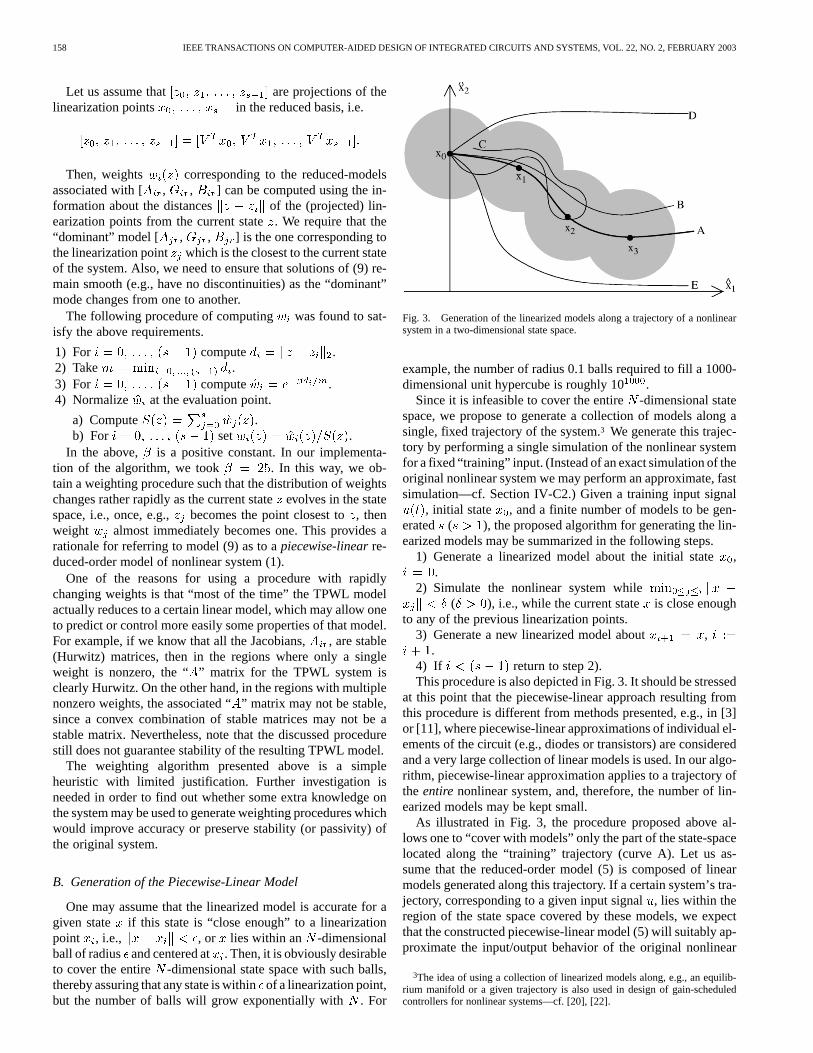
Fig. 3. Generation of the linearized models along a trajectory of a nonlinearsystem in a two-dimensional state space.

example, the number of radius 0.1 balls required to fill a 1000-dimensional unit hypercube is roughly 10 .

Since it is infeasible to cover the entire-dimensional statespace, we propose to generate a collection of models along asingle, fixed trajectory of the system.3 We generate this trajec-tory by performing a single simulation of the nonlinear systemfor a fixed “training” input. (Instead of an exact simulation of theoriginal nonlinear system we may perform an approximate, fastsimulation—cf. Section IV-C2.) Given a training input signal

, initial state , and a finite number of models to be gen-erated ( ), the proposed algorithm for generating the lin-earized models may be summarized in the following steps.

1) Generate a linearized model about the initial state,.

2) Simulate the nonlinear system while( ), i.e., while the current state is close enough

to any of the previous linearization points.3) Generate a new linearized model about ,

.4) If return to step 2).This procedure is also depicted in Fig. 3. It should be stressed

at this point that the piecewise-linear approach resulting fromthis procedure is different from methods presented, e.g., in [3]or [11], where piecewise-linear approximations of individual el-ements of the circuit (e.g., diodes or transistors) are consideredand a very large collection of linear models is used. In our algo-rithm, piecewise-linear approximation applies to a trajectory ofthe entire nonlinear system, and, therefore, the number of lin-earized models may be kept small.

As illustrated in Fig. 3, the procedure proposed above al-lows one to “cover with models” only the part of the state-spacelocated along the “training” trajectory (curve A). Let us as-sume that the reduced-order model (5) is composed of linearmodels generated along this trajectory. If a certain system’s tra-jectory, corresponding to a given input signal, lies within theregion of the state space covered by these models, we expectthat the constructed piecewise-linear model (5) will suitably ap-proximate the input/output behavior of the original nonlinear

3The idea of using a collection of linearized models along, e.g., an equilib-rium manifold or a given trajectory is also used in design of gain-scheduledcontrollers for nonlinear systems—cf. [20], [22].


Fig. 4. Comparison of system response (micromachined switch example)computed with linear, quadratic, and piecewise-linear reduced-order models(q = 40 andq = 41) to the step input voltageu(t) = 7H(t) [H(t) � 7 fort > 0 andH(t) � 0 for t < 0]. The piecewise-linear model was generatedfor the 8-V step input voltage.

system (cf. curves B and C).4 It should also be stressed at thispoint that, although the considered trajectory stays close to the“training” trajectory in the state space, the corresponding inputsignal can be dynamically very different from the “training”input. In other words, we may apply the piecewise-linear modelfor inputs which are significantly different from the “training”input, provided the corresponding trajectories stay in the regionof the state space covered by the linearized models (cf. curve Cand results in Section V). This case is also illustrated in Fig. 4,which shows computational results for the example of a mi-cromachined switch (cf. Section II). This figure presents thesystem response to a 7-V step input voltage, computed with a41st-order piecewise-linear reduced model of the device, gener-ated for an 8-V step input training voltage. (The model was gen-erated using the fast algorithm proposed in Section IV-C.) Weshould stress that, in fact, the input to the system is the squaredinput voltage . One may note that the obtainedoutput signal approximates very accurately the output signalcomputed with the full nonlinear model of the device (the curveson the graphs overlap almost perfectly). In this case, the piece-wise-linear model provides significantly more accurate resultsthan the linear or quadratic models based on single expansionsabout the initial state.

A different situation occurs when the input signal causes thetrajectory to leave the region covered by the linearized models(cf. curves D and E in Fig. 3). Then, the piecewise-linear model(5) will most likely not provide significantly better approxima-tion to the nonlinear system than a simple linear reduced model(6). This situation has been illustrated in Fig. 5. Due to a signif-icant difference in scales (amplitudes) between the “training”input and the testing input the piece-wise-linear model is no longer able to reproduce accurately the

4The additional rationale for this observation is that in typical situations thedimensions of observable and controllable spaces of a dynamical system aremuch lower than the dimension of its state space. (This is expected to be truefor the examples of nonlinear dynamical systems presented in Section II.)

Fig. 5. Comparison of system response (micromachined switch example)computed with linear, quadratic, and piecewise-linear reduced-order models(q = 40 and q = 41) to the step input voltageu(t) � 9 (t > 0). Thepiecewise-linear model was generated for the 7-V step input voltage.

Fig. 6. Comparison of system response (micromachined switch example)computed with linear, quadratic, and piecewise-linear reduced-order models(q = 40 and q = 41) to the step input voltageu(t) � 9 (t > 0). Thepiecewise-linear model was generated for the 9-V step input voltage.

response of the nonlinear system. Now, if we generate the piece-wise-linear model with a 9-V training input (cf. Fig. 6), then thismodel is able to reproduce accurately the nonlinear response.One should note that in this case the piecewise-linear modelis able to accurately model the dynamics of a highly-nonlinearpull-in effect (the beam is pulled down to the substrate), whichis of particular importance in applications [10]. One may notefrom the graph that the linear model is not able to reproduce thisphenomenon, while the quadratic model is unable to reproducethe correct dynamics. Still, this example shows that if the piece-wise-linear model is to be used for inputs with very differentscales one should consider more complicated schemes of gen-erating the linearized models, based, e.g., on multiple traininginputs.


C. Fast Generation of TPWL Models

The above method for generating piecewise-linear models ofnonlinear dynamical systems requires simulating the originalnonlinear system (1). This simulation can be costly, due to theoriginal size of the problem. In order to reduce the computa-tional effort, we note that it is unnecessary to compute theexacttrajectory for the “training” input in order to generate a col-lection of linearized models. In fact, it suffices to compute anapproximatetrajectory and obtain only approximate lineariza-tion points. In this section, we present an approach for efficientgeneration of piecewise-linear reduced-order models based onthis idea. The proposed numerical algorithm proceeds in the twostages: 1) generation of the reduced basis, used to represent ap-proximately the state space vectors () and 2) approximate sim-ulation of the nonlinear system response to the training input,using the reduced basis and piecewise-linear approximation ofthe nonlinear functions and along a trajectory of thenonlinear dynamical system (1). This approach shares featureswith reduced-basis methods for solving parabolic problems [5].Below, these two stages are described in more detail.

1) Generation of the Reduced Basis:The reduced-orderbasis , where , is obtained in thefollowing three steps.

1) Generate the linearization of the dynamical system (1) aboutthe initial state

(10)

where , and ( ) is the Jacobian of, evaluated at , and construct an orthogonal

basis in the th order Krylov subspace

(11)

using the Arnoldi algorithm [23] (or block Arnoldi algo-rithm [17] if the number of inputs ). This choiceof basis ensures that moments of the transfer functionof the reduced-orderlinearized model matchmoments ofthe transfer function for the original linearized model (10)[8], [15].

2) Orthonormalize the initial state vector with respect tothe columns of and obtain vector . (To this end,one may use e.g., the singular value decomposition (SVD)algorithm.)

3) Take as a union of and : .

So, the final size of the reduced basis equals . Thelast two steps ensure that we will be able to represent exactlythe initial state in the reduced basis . [Note that if

, then steps 2) and 3) become unnecessary.] Exactrepresentation of the initial state ensures that we may correctly

start the fast approximate simulation of the nonlinear system inthe reduced-order space as described in the following section.5

2) Fast Approximate Simulation:The second stage of theproposed MOR algorithm may be summarized in the followingsteps.

1) Take , set to be the initial state.2) While do

a) Using basis , construct a reduced-order model of dy-namical system (1), linearized about state

(12)where is a reduced-order approximation of state vector

( ). This step requires computation of the Ja-cobians and (at ) in the nonreduced statespace.

b) Simulate reduced-order linear dynamical system (12),i.e., compute for subsequent time steps ,while the state is close enough to the initial state

( ), i.e., when

where is an appropriately selected constant (cf. thecomments below).

c) Take the next linearization point ,.

There is an important issue concerning the TPWL MORalgorithm proposed above. In order to be able to reproducenonlinear effects in the behavior of a dynamical system, thelinearization points should be changed “frequently enough”during the proposed piecewise-linear simulation. This is deter-mined by the constant parameterin the algorithm presentedabove. The proper choice of was found to depend signifi-cantly on the amplitude of the input signal .

A simple procedure for determining an appropriate value ofautomatically is as follows. First, for a given input signal, we

perform a reduced-order simulation of the linearized dynamicalsystem, with linearization about the initial state, to find the final(steady–state) vector . Although in most cases will notbe the correct steady state of our nonlinear dynamical system, itwill give us information about the scale of changes between theinitial and final state

(If , we may take .) It is clear that in orderto capture any nonlinear effects one has to select the value ofsuch that . In practical situations, it is usually enough toselect or .

3) Generation of the Reduced Basis—An Extended Algo-rithm: The simple algorithm for generating the reduced-orderbasis, which constructed a Krylov subspace only at the initial

5In this section, we presented only the simplest (and the least computationallyexpensive) algorithm for generating the reduced basisV . One may easily extendthis scheme to construct a basis which includes e.g., states used as subsequentlinearization points and Krylov subspaces corresponding to these states. Suchan approach is presented in Section IV-C3.


state of the system, can be extended in order to include inthe reduced-order basis Krylov subspaces corresponding toother linearization points located along the training trajectory[19]. This extension of the reduced basis is motivated by thefollowing fact. As already mentioned in the previous section,if we use basis spanning Krylov subspace (11) to constructa linear reduced-order model, then the firstmoments ofthe transfer function for this reduced-order linear modelmatch first moments of the transfer function for the originallinearized model (10). Consequently, important dynamicalfeatures of the nonreduced linearized model are preserved bythe reduced-order linear model [8], [15]. Since in the TPWLmodel we use a collection of reduced-order linear models,taking a union of bases in Krylov subspaces corresponding tosubsequent linearized models as a reduced-order basiswillensure that, for every resulting reduced-order linear model,the first few moments of its transfer function will match thefirst few moments of the transfer function of the correspondingnonreduced-linearized model. Consequently, we may expectthat important dynamical properties for each of the linearizedmodels will be preserved after the projection process.

Two important technical details arise during the constructionof the union of bases at different linearization points. Firstly, ifwe linearize about a nonequilibrium point two input terms ap-pear (instead of one, if we linearize about an equilibrium)—oneassociated with term , and the other—associated withterm , where is a given linearizationpoint [cf. (12)]. Consequently, bases corresponding totwo different Krylov subspaces and

[cf. (11)] need to be con-structed. Secondly, we need to eliminate redundant (e.g., almostparallel) vectors (which may appear after we take a union of acollection of bases) from the reduced basis. To this end, we mayapply, e.g., SVD algorithm and discard vectors correspondingto the smallest singular values.

Using the above motivation, we developed an extendedalgorithm for generating the projection basis, which may besummarized in the following steps.

1) Let , .2) Repeat until the “training” simulation is completed.

a) Consider linearization of dynamical system (1) aboutstate

(13)

where is the Jacobian of , evaluated at ,is the Jacobian of evaluated at , and

and construct two orthogonal basesandin the following th order Krylov subspaces

using the Arnoldi algorithm [23] (or block Arnoldi al-gorithm [17] if there are multiple inputs).

b) Take as .c) Orthogonalize the columns of using the SVD al-

gorithm and construct a new basis which containsorthogonalized columns of corresponding to singularvalues larger than a given .

d) Take .e) Using , construct a linearized reduced-order system at

and simulate this system until you reach the next lin-earization point , set .

3) Orthogonalize the columns of the aggregate basisusingthe SVD algorithm and construct the final reduced-orderbasis which includes orthogonalized columns of cor-responding to singular values larger than some .

Step 2c) from the above algorithm may be omitted if wesimulate a full order nonlinear system (instead of a linearizedreduced-order system) in order to find subsequent linearizationpoints. Then, one should take .

One may note that the above method is more expensive thanthe simple algorithm presented earlier, since we need to gen-erate two orthogonal bases at every linearization point. To thisend, we need to perform LU factorization of Jacobiansatevery linearization point . In the simple approach, presentedin Section IV-C1, this had to be done only once. The extendedalgorithm also requires additional SVD steps.

Nevertheless, since we generate a “richer” basis we expectthat it will more adequately approximate the initial state space.One may argue though that the above method may generatemodels of significantly larger order than the simple algorithm.In fact, the situation is often the opposite. As shown in Sec-tion IV-C, the extended algorithm has potential to generate suit-able, accurate reduced bases with a lower order than the simplealgorithm using a single linearization about the initial state.

D. A Posteriori Error Estimation

In this section, we will present a method fora posterioriestimating the error of solving (1) with a TPWL model (9).The following derivation of the error estimator is based onthe assumption that the original nonlinear function[cf. (1)]is negative monotone, i.e., [24]:

(14)

The above assumption is satisfied by a number of nonlinearsystems, including, e.g., a certain class of nonlinear analogcircuits. Also, one may easily note that ifis negative monotone,then system (1) is stable for any admissible, provided

, where is a symmetric positive definite matrix.For simplicity, we will also assume in this section that

from (1) is an identity transformation and that . Still,the following derivation may be easily extended for the caseof an arbitrary invertible transformation (with appropri-ately modified assumptions) and a state-dependent input matrix

.


We will look for an estimate of , where, and and are solutions at

time of (1) and (9), respectively (for the same initial condition6 and the same input signal). From (1) and (9) we have

where , and . From the above weobtain

(15)

where

Since , for every , we may write

where and is the Hessian of .Then becomes

(16)

Left multiplying (15) by , and applying property (14) andSchwartz inequality gives

(17)Let us now consider time interval . Suppose we know

. Then, applying Comparison Lemma [9] to differen-tial inequality (17) yields

(18)

for all . The above inequality leads us to proposingthe following scheme of computing error estimates of

at time steps .

6If x cannot be represented exactly in basisV , the initial condition for thereduced system is taken asz = V x .

1) At we have, where is a known initial

condition.2) For we iteratively compute

(19)

Clearly, it follows from (18) that for every. In practice, we replace the supremum in the above formula by

a maximum over a discrete set of time steps betweenand ,corresponding to a certain numerical time integration scheme.(If are the same as subsequent integration steps, then we takea maximum of the two values at the ends of the considered timeinterval.) Clearly, this method of evaluating the supremum im-plicitly assumes that neither nor behave patholog-ically between subsequent integration time steps.

The main challenges associated with using the above schemeare related to: 1) finding [compare (14)] which would beas precise as possible. (Quality of the error estimates heavilydepends on this parameter, therefore, one could consider usingdifferent s in different regions of the state space, if at allpossible and computationally feasible.) and 2) finding estimatesof , given by (16), which typically requires estimating

—the norm of the Hessian of .If we apply the aggregate reduced-order basis, described

in Section IV-C3, then one may easily note that , forevery . Furthermore, if we include ( ) in thereduced basis , then[cf. (16)] and the following estimate of may be given:

Then, we may replace (19) with

(20)

One should note that since the values of norms(for every ) and can be

computed during construction of the reduced model, the cost ofevaluating (20) is only. This means that error estimationmay be performed “on the fly,” along with the reduced-ordersimulation, without increasing the complexity of the fast solver.


Fig. 7. Example of a circuit with quadratic nonlinearity.

In order to verify the proposed method of estimating the sim-ulation error for the TPWL reduced-order model, we consid-ered a simple test example of anRC ladder shown in Fig. 7.A quadratic nonlinearity is introduced to the circuit by addingnonlinear resistors to the ground at each node

where if and if . If wetake , then the nonlinear operator[cf. (1)]takes the following form:

where

......

.. .

and is the vector of states ( inour test). It may easily be proved thatis negative monotone,provided all are nonnegative at all times (which is satisfiedif the input current for all ). The value of [cf. (14)]may then be taken as , whereis the spectrum of matrix . For , .We also have that for all . Knowing and

we are ready to use formula (20) to compute errorestimates.

In a numerical test, we generated a reduced-order TPWLmodel of order (with linearization points)and simulated both original nonlinear system and TPWLreduced-order model, with the input current equal to unitstep. (It should be stressed thatis relatively large, as comparedto for this example, and, therefore, it may be inefficient touse the extracted TPWL model in practice. Still, this reducedmodel provides useful insight while considering the problem oferror estimation.) The actual error and its estimate werecomputed at every time step. Fig. 8 shows a comparison of theactual error and its estimate for the considered case. One maynote that formula (20) gives reasonable estimates of the errorof approximating the original nonlinear system with a TPWLreduced-order model.

One should note that the error estimation procedure describedabove may be used not only to assess errors of simulation withan existing TPWL reduced-order model, but also to improve thealgorithm for generating the TPWL models (or, more precisely,the algorithm for selecting subsequent linearization points).Currently, during the “training simulation,” the subsequentlinearization points are selected using a simple geometriccriterion: if the current state is “far enough” from all previouslinearization points, then it becomes the next linearization

Fig. 8. A posteriori error estimates for a TPWL reduced-order model of anonlinearRC ladder.

Fig. 9. Comparison of system response (nonlinear transmission line circuitmodel) computed with linear, quadratic, full nonlinear, and TPWL models tothe step input currenti(t) = H(t � 3) [H(t) � 1 for t > 3 andH(t) � 0for t < 3]. N = 1500.

point. Instead of this geometric criterion, perhaps one mightuse a measure based on error estimates (which use informationon the nonlinear system at hand) to select a collection oflinearization points. Clearly, the subject of where to placelinearization points needs further investigation.

V. FAST PIECEWISE-LINEAR SIMULATOR

One should note that the MOR algorithm presented inSection IV-C may be used as a fast simulator for nonlineardynamical systems. The simulator has been implemented forthe example of a nonlinear transmission line circuit modeldescribed in Section II. Selected results of numerical tests arepresented below.

Fig. 9 shows the output voltage for a step input current,computed using full order linear and quadratic models as well as


TABLE IQUALITY OF APPROXIMATION FOR LINEAR, QUADRATIC AND

TPWL SIMULATORS FOR THE STEP INPUT CURRENT.v = [v(0); v(�T ); . . . ; v(T )] IS THE COMPUTED

OUTPUT VOLTAGE AT NODE 1, v IS THE

REFERENCE OUTPUT VOLTAGE COMPUTED

WITH FULL NONLINEAR MODEL

TABLE IICOMPARISON OFSIMULATION TIMES FOR THEFULL ORDER NONLINEAR

SIMULATOR AND THE PROPOSEDTPWL REDUCEDORDERSIMULATOR

the proposed TPWL simulator. The reference result is computedwith a simulator using a full order nonlinear model. In the simu-lation the number of time steps was 1000 ( , ),the TPWL simulator used the reduced basis of order (theoriginal problem size was ) and the linearization pointchanged 20 times (i.e., it used 21 different linear models duringthe simulation). As Fig. 9 clearly shows, the output voltage ob-tained by the TPWL method matches very well the reference re-sult (the curves overlap almost perfectly). Table I shows the rel-ative error between the voltagecomputed with linear, quadratic, and TPWL simulators and thereference voltage obtained with the full nonlinear model ofthe circuit. It is apparent that the proposed piecewise-linear al-gorithm gives significantly more accurate results than the linearor quadratic simulations, producing results which accuratelymatch the steady state of the system.

Table II compares performance of the full nonlinear simulatorfor the considered nonlinear transmission line circuit modeland the proposed TPWL solver, which performs reduced-basiscomputations, for three different inputs. In order to assureappropriate accuracy, for the circuit with nodes, theorder of the reduced basis equaled , and for the circuitwith , . The simulators were implementedin Matlab, therefore, the presented execution times should beused for comparison only. High-performance implementationswill most likely give significantly lower absolute executiontimes and may change the relative performance of the twoalgorithms. The tests were performed on a Linux workstationwith a Pentium III Xeon processor. It is apparent that for eithersmall or large original problem sizes, the piecewise-linearsimulator is significantly faster than the full nonlinear solver.For , a hundredfold acceleration in computation timewas achieved.

Fig. 10. Comparison of system response (nonlinear transmission line circuitmodel) computed with linear, quadratic, and TPWL reduced-order models (oforderq = 10) for the step input currenti(t) = H(t� 3) [H(t) � 1 for t > 3andH(t) � 0 for t < 3]. The TPWL model was generated using a unit stepinput current.

VI. COMPUTATIONAL RESULTS

A. Model Verification—Transient Simulations

This section presents results of computations using TPWLreduced-order models, obtained with the MOR technique pro-posed in Section IV-C. Our main goal is to find out whether thistechnique does really generatea modelof our system. Let usrecall that, in the proposed MOR algorithm, the model [whichbasically consists of a collection of reduced-order matrices

] is obtained by performing a fastsimulation for agiventraining input signal. In order to show thatwe have indeed generated a model we should verify that it givescorrect outputs not only for the input it was generated with, butalso for other inputs.

This verification was done experimentally. We consideredour nonlinear transmission line circuit model (cf. Section II)with nodes and generated a reduced-order TPWLmodel of order using a step input .For this example, the linearization point changed four times,therefore, our model consisted of five reduced-order matrices

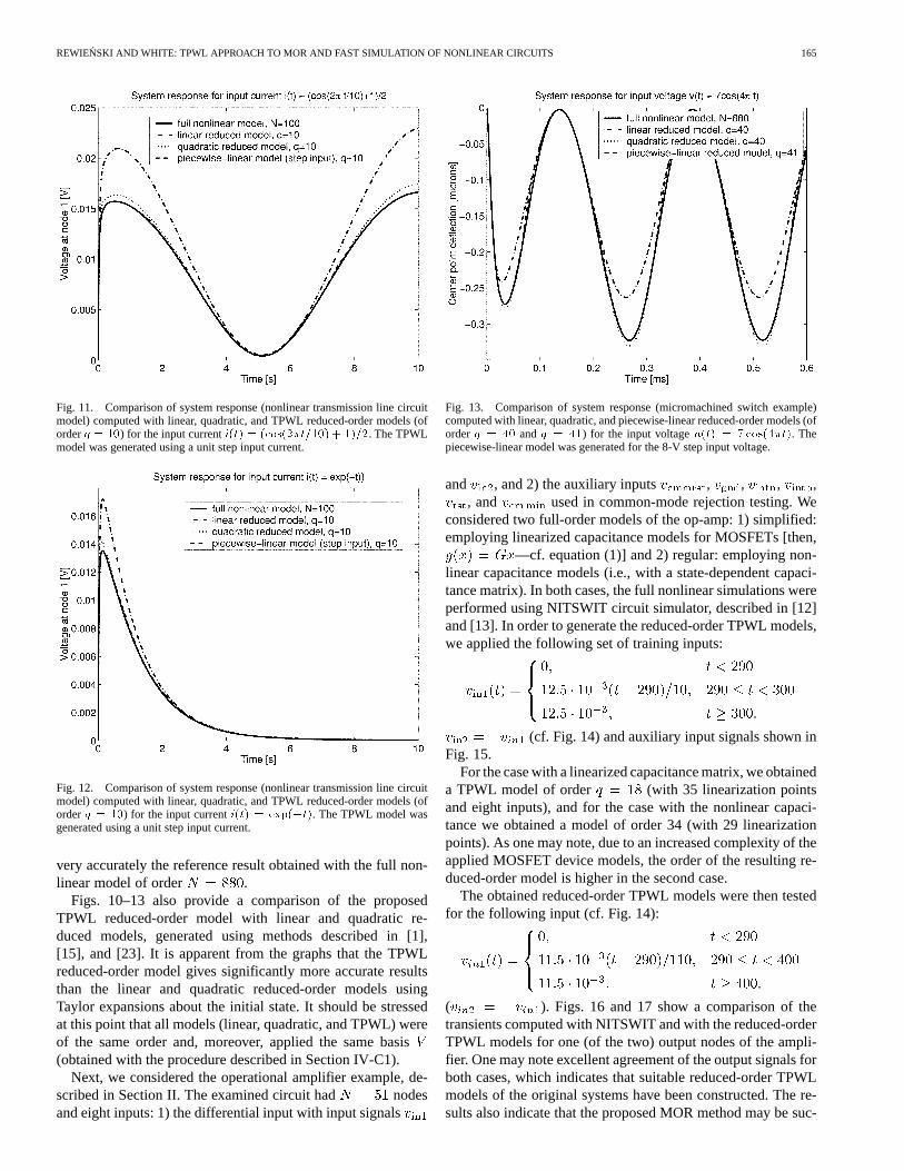
. The reduced-order model was tested for differentinputs, including the step input used to generate it. Fig. 10 showsthe result for the step input (the same input we used for modelextraction). Figs. 11 and 12 show the reduced-order simulationresults for a cosinusoidal input and an exponentially decayinginput, respectively. In all the cases, the output voltages obtainedwith the TPWL reduced-order model accurately approximatethe reference voltages (the curves overlap almost perfectly).This indicates that our reduced-order system provides a sensiblemodel for the original nonlinear circuit.

Fig. 13 provides an analogous test for the example of a mi-cromachined beam described in Section II. In this case, the re-duced-order model was generated for the step 8-V training inputvoltage ( , the model used nine linearization points. Thenit was tested for a cosinusoidal input with a 7-V amplitude. Onceagain, the transient obtained with the TPWL model matches


Fig. 11. Comparison of system response (nonlinear transmission line circuitmodel) computed with linear, quadratic, and TPWL reduced-order models (oforderq = 10) for the input currenti(t) = (cos(2�t=10) + 1)=2. The TPWLmodel was generated using a unit step input current.

Fig. 12. Comparison of system response (nonlinear transmission line circuitmodel) computed with linear, quadratic, and TPWL reduced-order models (oforderq = 10) for the input currenti(t) = exp(�t). The TPWL model wasgenerated using a unit step input current.

very accurately the reference result obtained with the full non-linear model of order .

Figs. 10–13 also provide a comparison of the proposedTPWL reduced-order model with linear and quadratic re-duced models, generated using methods described in [1],[15], and [23]. It is apparent from the graphs that the TPWLreduced-order model gives significantly more accurate resultsthan the linear and quadratic reduced-order models usingTaylor expansions about the initial state. It should be stressedat this point that all models (linear, quadratic, and TPWL) wereof the same order and, moreover, applied the same basis(obtained with the procedure described in Section IV-C1).

Next, we considered the operational amplifier example, de-scribed in Section II. The examined circuit had nodesand eight inputs: 1) the differential input with input signals

Fig. 13. Comparison of system response (micromachined switch example)computed with linear, quadratic, and piecewise-linear reduced-order models (oforderq = 40 andq = 41) for the input voltageu(t) = 7 cos(4�t). Thepiecewise-linear model was generated for the 8-V step input voltage.

and , and 2) the auxiliary inputs , , , ,, and used in common-mode rejection testing. We

considered two full-order models of the op-amp: 1) simplified:employing linearized capacitance models for MOSFETs [then,

—cf. equation (1)] and 2) regular: employing non-linear capacitance models (i.e., with a state-dependent capaci-tance matrix). In both cases, the full nonlinear simulations wereperformed using NITSWIT circuit simulator, described in [12]and [13]. In order to generate the reduced-order TPWL models,we applied the following set of training inputs:

.

(cf. Fig. 14) and auxiliary input signals shown inFig. 15.

For the case with a linearized capacitance matrix, we obtaineda TPWL model of order (with 35 linearization pointsand eight inputs), and for the case with the nonlinear capaci-tance we obtained a model of order 34 (with 29 linearizationpoints). As one may note, due to an increased complexity of theapplied MOSFET device models, the order of the resulting re-duced-order model is higher in the second case.

The obtained reduced-order TPWL models were then testedfor the following input (cf. Fig. 14):

.

( ). Figs. 16 and 17 show a comparison of thetransients computed with NITSWIT and with the reduced-orderTPWL models for one (of the two) output nodes of the ampli-fier. One may note excellent agreement of the output signals forboth cases, which indicates that suitable reduced-order TPWLmodels of the original systems have been constructed. The re-sults also indicate that the proposed MOR method may be suc-


Fig. 14. Op-amp input signalsv andv .

Fig. 15. Auxiliary inputs for the op-amp circuit.

Fig. 16. Comparison of the output voltage (op-amp example, simplifiedlinearized capacitance models), computed with a reduced-order TPWL modeland NITSWIT circuit simulator.

Fig. 17. Comparison of the output voltage (op-amp example, regularnonlinear capacitance models), computed with a reduced-order TPWL modeland NITSWIT circuit simulator.

TABLE IIICOMPARISON OF THETIMES OF MODEL EXTRACTION AND REDUCED

ORDER SIMULATION FOR THE LINEAR, QUADRATIC AND TPWLMOR TECHNIQUES. THE ORIGINAL PROBLEM HAD SIZE

N = 1500. THE REDUCED MODEL HAD SIZE

q = 30. THE TESTS WERE RUN FOR THE

NONLINEAR TRANSMISSIONLINE EXAMPLE

cessfully used for multiple input systems. It is important to pointout that not only do the TPWL models have a lower order thanthe original system, but also they are much easier to use. Sincea TPWL model consists of a weighted combination of linearmodels, the time stepping is very straightforward. In a simplifiedbackward Euler time stepping scheme we compute the weights

[cf. (9)] e.g., using the previous state of the system or a pre-dictor of the next state and then, assuming that these weights arefixed, we find the state at the next time step by performing only asingle Newton update (i.e., solving a low-order linear system ofequations). In a more sophisticated time stepping scheme, onecan account for derivatives of , which is also straightfor-ward, since the weights are simple scalar functions. In a regularsimulator, if using backward Euler scheme, finding the next staterequires computation of a number of Newton updates for the fullorder nonlinear system, which is considerably more complex.

B. Performance and Complexity of the MOR Algorithm

Table III shows a comparison of the performance of the dis-cussed MOR techniques and the reduced-order solvers. All thealgorithms were implemented in Matlab. The tests were per-formed on a Linux workstation with a Pentium III Xeon pro-cessor. One may note that performance for linear and TPWLmodels is comparable. The generation of the quadratic modelis significantly more expensive, due to the costly reduction of


Fig. 18. Comparison of system response (micromachined switch example)computed using the TPWL models extracted with the simple and the extendedalgorithm for generating the reduced-order basis. In both cases, the models weregenerated for the 5.5-V step input voltage.

the Hessian matrix, which requires computations of the ma-trix-vector product , where is a full orderHessian matrix (usually represented implicitly—cf. [1]).

The memory complexity of the TPWL reduced-order solveris , where is the number of linearization points. Conse-quently, the memory cost is roughlytimes larger than the costfor the linear reduced-order simulator [which is ]. Thememory cost of the quadratic reduced-order solver is (thereduced-order Hessian must be stored explicitly as a matrix), soif , then the memory requirements for the piecewise-linearsolver are approximately the same as for the quadratic solver.For the examples of the nonlinear transmission line and the mi-cromachined switch (cf. Figs. 10–13, or

), so in those cases the memory used by the piece-wise-linear algorithm equaled roughly only half (or a quarter) ofthe memory used by the quadratic solver. In the case of the op-erational amplifier (linearized capacitance case), whichtranslates to doubled storage requirements as compared to thequadratic model.

C. Performance of the Extended Algorithm for Generating theReduced-Order Basis

This section presents computational results comparing twoalgorithms for generating the reduced-order basis: a simple one,presented in Section IV-C1, and the extended one, introduced inSection IV-C3. Fig. 18 shows the deflection of the center of themicromachined fixed–fixed beam computed using the two con-sidered methods. In both MOR methods, the 5.5-V step inputvoltage was used as a “training” input and the number of lin-earization points equaled six. For the simple algorithm, the orderof the reduced-model equaled . In the extended algo-rithm, a basis of order seven [ , —cf. Step2)a) in the algorithm from Section IV-C3] was generated at eachof the linearization points. Then the size of the aggregate basis

has been reduced from to 28 using the SVD al-gorithm. One may note that the TPWL model of order ,

Fig. 19. Comparison of system response (micromachined switch example)computed using the full nonlinear simulator and the TPWL reduced-order modelextracted with the simple algorithm for generating the reduced-order basis. Themodel of orderq = 41 was generated for the 5.5-V step input voltage.

Fig. 20. Comparison of system response (micromachined switch example)computed with different MOR algorithms. TPWL models were generated forthe 9-V step input voltage.

generated with the extended reduced-order basis, gives signif-icantly more accurate results than the TPWL model generatedwith a simple basis. (On the graph, the dashed line overlaps per-fectly with the solid line.) In order to obtain the desired accuracywith the model extracted with the simple basis generation algo-rithm, the order of the basis needs to be increased to inthe considered case (cf. Fig. 19).

Fig. 20 shows the simulated pull-in effect for the microma-chined switch example. Again, in this case, the MOR methodemploying the extended algorithm to generate the reduced basisprovides the best accuracy among the considered MOR tech-niques. It also generates a model with the lowest order.

One should note that in the extended algorithm, we generatea collection of very-low-order bases at different linearizationpoints rather than a larger basis at a single linearization point, asin the initial approach. As shown by the presented results, this


TABLE IVCOMPARISON OF THETIMES OF MODEL EXTRACTION AND REDUCED ORDER

SIMULATION FOR THE TPWL MOR ALGORITHMS USING TWO DIFFERENT

METHODS OFGENERATING THE REDUCED ORDER BASIS. THE TESTS

WERE RUN FOR THE MICROMACHINED SWITCH EXAMPLE. THE

ORIGINAL PROBLEM SIZE EQUALED N = 880

Fig. 21. Comparison of sinusoidal steady state (nonlinear transmission linecircuit model) computed using full nonlinear and TPWL models. The inputsignal wasi(t) = (cos(2�t) + 1)=2.

may lead to a model with a lower order, which is faster to simu-late. The tradeoff is that the extended basis generation algorithmis computationally more expensive. This has been illustrated inTable IV, which shows performance of the MOR techniques forthe considered micromachined beam example.

D. Sinusoidal Steady–State Simulations

This section compares results of simulation of the sinusoidalsteady state computed with the full-order nonlinear models andthe reduced-order TPWL models. The tests were performed forthe examples of a nonlinear transmission line circuit model (cf.Fig. 1) and the operational amplifier, described in Section II.

In the first series of tests, we computed the sinusoidal steadystate for the nonlinear transmission line model withnodes, excited with the input current .The simulation was performed with a simple, fixed time stepshooting method. Fig. 21 shows the computed sinusoidalsteady–state output of the system in time domain. One maynote that the result obtained with the reduced-order model oforder closely matches the reference result.

The frequency domain analysis has also been performed forthe sinusoidal steady–state output signal shown in Fig. 21.[ , where is the voltage at node 1 of the cir-cuit.] We computed a complex discrete Fourier transform (DFT)

TABLE VCOMPARISON OF THESUBSEQUENTHARMONICS OF THESINUSOIDAL

STEADY STATE, COMPUTED USING A FULL ORDER NONLINEAR

MODEL AND THE REDUCED ORDER TPWL MODEL

TABLE VICOMPARISON OF THEMAIN INTERMODULATION HARMONICS OF THE

SINUSOIDAL STEADY STATE, COMPUTED USING A FULL-ORDER

NONLINEAR MODEL AND THE REDUCED ORDER

TPWL MODEL (q = 39)

of the discrete output signal . The first fourFourier coefficients (not normalized) are shown in Table V.One may note that the sinusoidal steady stateobtained withthe discussed reduced-order model matches closely up to thethird harmonic of the reference sinusoidal steady state of theconsidered nonlinear transmission line model. This result sug-gests that the extracted reduced-order models may be used toanalyze second-order effects like harmonic distortion.

In a different series of tests, we applied a TPWL reduced-order model to compute intermodulation distortion for the con-sidered op-amp example (using nonlinear capacitance modelsfor MOSFETs). We generated two TPWL models: the first oneof order (with 39 linearization points), and the secondone of order (with 36 linearization points) for a sinu-soidal training input (which was the same in both cases)

where MHz. Then, the models were tested for the inputsignal being a sum of two sinusoids with different frequencies:

where MHz and MHz, and the spectrum ofthe computed sinusoidal steady state was extracted using DFT.Tables VI and VII show the complex amplitudes of the main in-termodulation products and the driving harmonics obtained withthe TPWL reduced-order models and the full nonlinear modelof the considered op-amp. The error shown in the tables is therelative error of the computed amplitude. The results indicatethat the TPWL reduced model is able to effectively reproducethe intermodulation distortion effects in the considered case. Atthe same time, comparison between the two tables shows that


TABLE VIICOMPARISON OF THEMAIN INTERMODULATION HARMONICS OF THE

SINUSOIDAL STEADY STATE, COMPUTED USING A FULL ORDER

NONLINEAR MODEL AND THE REDUCED ORDER

TPWL MODEL (q = 35)

the computed amplitudes of intermodulation products vary sig-nificantly depending on the applied TPWL model which sug-gests that in this case we may not further reduce the order of themacromodel.

VII. CONCLUSION

In this paper, we have proposed an efficient numericalapproach for MOR and simulation of nonlinear dynamicalsystems. The results obtained for the examples of nonlinearcircuits and a micromachined switch indicate that the presentedmethod provides very good accuracy for different applications(and both single- and multiple-input systems). The method alsoproves to be characterized by low computational and memoryrequirements, therefore, providing a cost-efficient alternativefor the nonlinear MOR techniques based on linear and quadraticmodels.

Although the algorithm in its current state has proved to bevery effective, its performance still depends on a few param-eters, which need to be adjusted more or less arbitrarily for agiven application example. The discussed parameters are relatedmainly to the weighting procedure, as well as the method ofselecting subsequent linearization points. Consequently, furtherdevelopments of the proposed MOR algorithm are necessary inorder to achieve its true robustness. Topics for further investi-gation include e.g.: 1) developing more sophisticated weightingprocedures which would exploit available information on theoriginal system in order to obtain more accurate TPWL modelsand/or to preserve stability or passivity of the original system;2) incorporatinga posteriorierror estimation procedures to thealgorithm of selecting the collection of linearization points; and3) controlling approximation errors in the proposed fast simu-lation algorithm. A separate problem is to define what is an op-timal training input for a given nonlinear system.

There are also many possible extensions of the presentedMOR technique, which may include applying different typesof bases in the reduced-order TPWL simulators or devel-oping schemes for automatic model generation with multiple“training” inputs, which may allow one to extend the validity ofthe quasipiecewise-linear reduced-order model to inputs withdifferent scales of amplitudes. One should also note that appli-

cation of the discussed TPWL MOR approach is not limitedto single-input single-output or multiple-input multiple-outputdynamical systems given in form (1). For instance, if we extendthe weighting procedure to take into account not only the statespace of the system, but also the space of input signals, we maybe able to construct TPWL macromodels for systems with fullynonlinear input operators.

ACKNOWLEDGMENT

The authors would like to thank the anonymous reviewers forsuggestions that substantially improved the paper. In particular,the reviewers recommended extending the TPWL algorithm tothe case with nonlinear capacitors. They also suggested exam-ining intermodulation distortion.

REFERENCES

[1] Y. Chen and J. White, “A quadratic method for nonlinear model order re-duction,” inProc. Int. Conf. Modeling and Simulation of Microsystems,2000, pp. 477–480.

[2] J. Chen and S.-M. Kang, “An algorithm for automatic model-order re-duction of nonlinear MEMS devices,” inProc. IEEE Int. Symp. Circuitsand Syst., vol. 2, 2000, pp. 445–448.

[3] C. T. Dikmen, M. M. Alaybeyi, S. T. A. Atalar, E. Sezer, M. A. Tan,and R. A. Rohrer, “Piecewise linear asymptotic waveform evaluation fortransient simulation of electronic circuits,” inProc. Int. Symp. Circuitsand Syst., vol. 2, Singapore, 1991, pp. 854–857.

[4] P. Feldmann and R. W. Freund, “Efficient linear circuit analysis by Padéapproximation via the Lanczos process,”IEEE Trans. Computer-AidedDesign, vol. 14, pp. 639–649, May 1995.

[5] E. Gallopoulos and Y. Saad, “Efficient solution of parabolic equationsby Krylov approximation methods,”SIAM J. Sci. Stat. Comput., vol. 13,no. 5, pp. 1236–1264, 1992.

[6] K. Glover, “All optimal Hankel-norm approximations of linear multi-variable systems and theirL error bounds,”Int. J. Control, vol. 39,no. 6, pp. 1115–1193, 1984.

[7] E. J. Grimme, D. C. Sorensen, and P. Van Dooren, “Model reduction ofstate space systems via an implicitly restarted Lanczos method,”Numer.Algorithms, vol. 12, no. 1–2, pp. 1–31, 1996.

[8] E. J. Grimme, “Krylov projection methods for model reduction,” Ph.D.dissertation, Univ. Illinois, Urbana-Champaign, IL, 1997.

[9] J. K. Hale,Ordinary Differential Equations. New York: Wiley, 1969.[10] E. Hung, Y. Yang, and S. Senturia, “Low-order models for fast dynam-

ical simulation of MEMS microstructures,” inProc. IEEE Int. Conf.Solid-State Sensors and Actuators (Transducers ’97), vol. 2, 1997, pp.1101–1104.

[11] R. Kao and M. Horowitz, “Timing analysis for piecewise linear Rsim,”IEEE Trans. Computer-Aided Design, vol. 13, pp. 1498–1512, Dec.1994.

[12] K. Kundert, J. White, and A. Sangiovanni-Vincentelli, “A mixed fre-quency-time approach for finding the steady-state solution of clockedanalog circuits,” inProc. IEEE Custom Integrated Circuits Conf., 1988,pp. 6.2/1–6.2/4.

[13] , “A mixed frequency-time approach for distortion analysis ofswitching filter circuits,” IEEE J. Solid-State Circuits, vol. 24, pp.443–451, Apr., 1989.

[14] A. Odabasioglu, M. Celik, and L. Pileggi, “PRIMA: Passive reduced-order interconnect macromodeling algorithm,” inProc. IEEE/ACM Int.Conf. Computer-Aided Design, 1997, pp. 58–65.

[15] J. R. Phillips, “Automated extraction of nonlinear circuit macromodels,”in Proc. Custom Integrated Circuit Conf., 2000, pp. 451–454.

[16] , “Model reduction of time-varying systems using approximatemultipoint Krylov-subspace projectors,” inProc. IEEE/ACM Int. Conf.Computer-Aided Design, 1998, pp. 96–102.

[17] D. Ramaswamy, “Automatic generation of macromodels for MicroElec-troMechanical Systems (MEMS),” Ph.D. dissertation, MassachusettsInst. Technol., Cambridge, MA, 2001.


[18] M. Rewienski and J. White, “A trajectory piecewise-linear approach tomodel order reduction and fast simulation of nonlinear circuits and mi-cromachined devices,” inProc. Int. Conf. Computer-Aided Design, vol.1, 2001, pp. 252–257.

[19] , “Improving trajectory piecewise-linear approach to nonlinearmodel order reduction for micromachined devices using an aggregatedprojection basis,” inProc. 5th Int. Conf. Modeling and Simulation ofMicrosystems, vol. 1, 2002, pp. 128–131.

[20] J. S. Shamma, “Analysis and design of gain scheduled control systems,”Ph.D. dissertation, Massachusetts Inst. Technol., Cambridge, MA, 1988.

[21] L. M. Silveira, M. Kamon, and J. White, “Efficient reduced-order mod-eling of frequency-dependent coupling inductances associated with 3-Dinterconnect structures,” inProc. European Design and Test Conf., 1995,pp. 534–538.

[22] D. J. Stilwell and W. J. Rugh, “Interpolation methods for gain sched-uling,” in Proc. 37th IEEE Conf. Decision and Control, vol. 3, 1998, pp.3003–3008.

[23] F. Wang and J. White, “Automatic model order reduction of a microde-vice using the Arnoldi approach,” inProc. Int. Mechanical EngineeringCongr. and Exposition, 1998, pp. 527–530.

[24] J. K. White and A. Sangiovanni-Vincentelli,Relaxation Techniques forthe Simulation of VLSI Circuits. Norwell, MA: Kluwer, 1987.

[25] K. E. Willcox, J. D. Paduano, J. Peraire, and K. C. Hall, “Low orderaerodynamic models for aeroelastic control of turbomachines,” inProc.Amer. Inst. Aeronautics Astronautics Structures, Structural Dynamics,Materials Conf., vol. 3, 1999, pp. 2204–2214.

Michał Rewienski received the M.S. degree in com-puter science and the Ph.D. degree in electrical en-gineering from the Technical University of Gdansk,Gdansk, Poland, in 1998 and 2000, respectively.

He is currently a Research Assistant in theComputational Prototyping Group, Department ofElectrical Engineering and Computer Science, Mass-achusetts Institute of Technology, Cambridge. Hisresearch interests include developing fast numericalalgorithms for full-wave modeling and simulation ofelectromagnetic systems in high frequencies, MOR

techniques for nonlinear dynamical systems, and large-scale parallel scientificcomputing.

Jacob White (A’88) received the B.S. degreefrom the Massachusetts Institute of Technology,Cambridge, in 1980, and the S.M. and Ph.D. degreesfrom the University of California, Berkeley, in 1983and 1985, respectively, all in electrical engineeringand computer science.

He was with the IBM T. J. Watson ResearchCenter from 1985 to 1987, was the Analog DevicesCareer Development Assistant Professor at theMassachusetts Institute of Technology from 1987to 1989, and was a 1988 Presidential Young Investi-

gator. He is currently a Professor at the Massachusetts Institute of Technologyand an Associate Director of the Research Laboratory of Electronics. Hiscurrent research interests are in numerical algorithms for problems in circuit,interconnect and microelectromechanical system design.

Prof. White was an Associate Editor of the IEEE TRANSACTIONS ON

COMPUTER-AIDED DESIGN, from 1992 until 1996, and was Technical ProgramChair of the International Conference on Computer-Aided Design in 1998.

Documents

A trajectory piecewise-linear approach to model order ... Trajectory Piecewise-Linear Approach to Model Order Reduction and Fast Simulation of Nonlinear Circuits and Micromachined