Linköping Studies in Science and Technology Licentiate Thesis No. 1205

A Traffic Simulation Modeling Framework for Rural Highways

Andreas Tapani

LiU-TEK-LIC-2005:60

Department of Science and Technology

Linköpings Universitet, SE-601 74 Norrköping, Sweden

Norrköping 2005

A Traffic Simulation Modeling Framework for Rural Highways © Andreas Tapani, 2005 andta@itn.liu.se Thesis Number: LIU-TEK-LIC-2005:60 ISBN 91-85457-59-0 ISSN 0280-7971 Linköping University Department of Science and Technology SE-601 74 Norrköping, Sweden Tel: +46 11 36 30 00 Fax: +46 11 36 32 70

i

Abstract Models based on micro-simulation of traffic flows have proven to be useful tools in the study of various traffic systems. Today, there is a wealth of traffic micro-simulation models developed for freeway and urban street networks. The road mileage is however in many countries dominated by rural highways. Hence, there is a need for rural road traffic simulation models capable of assessing the per-formance of such road environments. This thesis introduces a versatile traffic mi-cro-simulation model for the rural roads of today and of the future. The developed model system considers all common types of rural roads including effects of inter-sections and roundabouts on the main road traffic. The model is calibrated and validated through a simulation study comparing a two-lane highway to rural road designs with separated oncoming traffic lanes. A good general agreement between the simulation results and the field data is established.

The interest in road safety and the environmental impact of traffic is growing. Recent research has indicated that traffic simulation can be of use in these areas as well as in traditional capacity and level-of-service studies. In the road safety area more attention is turning towards active safety improving countermeasures de-signed to improve road safety by reducing the number of driver errors and the accident risks. One important example is Advanced Driver Assistance Systems (ADAS). The potential to use traffic simulation to evaluate the road safety effects of ADAS is investigated in the last part of this thesis. A car-following model for simulation of traffic including ADAS-equipped vehicles is proposed and the de-veloped simulation framework is used to study important properties of a traffic simulation model to be used for safety evaluation of ADAS. Driver behavior for ADAS-equipped vehicles has usually not been considered in simulation studies including ADAS-equipped vehicles. The work in this thesis does however indi-cate that modeling of the behavior of drivers in ADAS-equipped vehicles is essen-tial for reliable conclusions on the road safety effects of ADAS.

iii

Acknowledgements This thesis would not have been completed without the guidance and support of my supervisor Jan Lundgren. Thank you Jan! No problem has been too big or small to discuss with you.

I would also like to express my gratitude towards Pontus Matstoms for intro-ducing me to the field of traffic simulation and to Arne Carlsson for his invaluable knowledge in traffic flow modeling and traffic engineering.

I have shared my time between VTI and the Communications and Transport Systems group at the University. Everyone at VTI and in the Communications and Transport Systems group has made this a truly inspiring environment to work in. I would especially like to thank my roommate Johan Janson Olstam for our fre-quent and fruitful discussions.

Finally, I would like to take this opportunity to show my appreciation for my family and friends. Thank you for always believing in me! Last but not least, thank you Erika for all the love and support. Linköping, October 2005 Andreas Tapani

v

Contents 1. Introduction 1 1.1 Problem Description 2 1.2 Objectives and Delimitations 2 1.3 Contribution 3 1.4 Outline 3

2. Rural Road Traffic Simulation 5 2.1 Introduction to Traffic Simulation 5 2.2 Sub-Models for Rural Road Traffic Simulation 7 2.2.1 Traffic generation 7 2.2.2 Speed-adaptation 8 2.2.3 Car-following 9 2.2.4 Overtakings 13 2.2.5 Intersection movements 14 2.3 State-of-the-Art Review 15 2.3.1 TRARR 16 2.3.2 TWOPAS 17 2.3.3 VTISim 18 2.3.4 Summary and conclusions 19

3. The Rural Traffic Simulator 21 3.1 Simulation Framework 21 3.2 Road Representation 24 3.2.1 Road data 24 3.2.2 Lanes and tracks 25 3.2.3 Sight distance function 26 3.2.4 Speed profile 26 3.3 Traffic Generation 34 3.3.1 Traffic data 34 3.3.2 Vehicle characteristics 35 3.3.3 Platoon generation 36 3.3.4 Generation of vehicle characteristics 39 3.4 Vehicle Movements 40 3.4.1 Acceleration model 40 3.4.2 Overtaking model 44 3.4.3 Intersections and roundabouts 50 3.4.4 Vehicle loading and unloading 52 3.5 Comparison Between VTISim and RuTSim 53 3.6 Implementation 54 3.6.1 Structure 54 3.6.2 Graphical user interface 56 3.6.3 Input 56 3.6.4 Output 56 3.6.5 Model verification 57

4. Rural Highway Design Analysis using RuTSim 59 4.1 Introduction 59 4.2 Study Site 59 4.2.1 Existing road and proposed road design alternatives 59

vi

4.2.2 Traffic volumes 60 4.3 Calibration and Validation of the RuTSim Model 61 4.3.1 Simulation models of the study site 61 4.3.2 Calibration and validation results 61 4.4 Analysis of Rural Road Design Alternatives 63 4.4.1 Journey speeds 64 4.4.2 Platoon lengths 67 4.5 Conclusions 68

5. Evaluation of Safety Effects of Driver Assistance Systems through Traffic Simulation 71

5.1 Introduction 71 5.2 Advanced Driver Assistance Systems and Safety Related Traffic

Measures 72 5.2.1 Advanced driver assistance systems 72 5.2.2 Safety related traffic measures 73 5.3 A Car-Following Model for Evaluation of ADAS 75 5.3.1 Model requirements 75 5.3.2 A model to be used in simulation of ADAS-equipped vehicles 76 5.4 Computational Results 77 5.4.1 Implementation 78 5.4.2 Simulation runs 78 5.5 Conclusions 83

6. Concluding Remarks and Future Research 85

References 87 Appendices A. Overtaking Parameters

B. Critical Time Gaps

C. Default Parameter Values

1

1. Introduction The main motivation for standard improvements in the traffic system has always been to increase capacity and the level-of-service. Today more attention is turning towards other issues such as road safety and the environmental impact of traffic. One important example of this paradigm change is the separation of oncoming lanes on major rural highways in Sweden. The separation of oncoming lanes on a highway will restrict traffic and may consequently reduce the level-of-service on the highway. Oncoming lane separation has on the other hand proven to improve the road safety substantially (Carlsson and Brüde, 2005). Another example of the increased road safety awareness is the growing use of rural roundabouts in Swe-den. Roundabouts will increase safety but at the same time reduce the level-of-service on the main road.

There is an increasing interest in traffic simulation as a tool for evaluation of traffic systems. Many simulation studies of the design of urban street networks and freeway operations have been conducted. The road mileage is however in most countries dominated by rural highways. So far, the use of traffic simulation for rural highways has not increased as much as the use of simulation for other road types. One reason for this difference is the focus on urban and freeway con-gestion within the modeling community. Today’s growing awareness of other issues such as road safety and the environment has however also brought an in-creasing interest in the performance of rural highways. Since traffic simulation has proven to be a useful tool for other road environments there is also a potential to use traffic simulation for rural roads to a greater extent than today.

Simulation is also likely to become more and more essential in studies of all types of road environments. The nature of the traffic system is continuously changing, new vehicle and infrastructure technology creates new traffic condi-tions. At the moment, Intelligent Transportation Systems (ITS) are becoming an increasingly important element in the traffic system. ITS are technology based applications designed to improve several aspects of traffic and transport systems. These applications increase the complexity of the interactions between individual vehicles and the surrounding traffic and between vehicles and the infrastructure. Simulation is a powerful method for studies of complex systems. Nevertheless, to account for the ever changing traffic system there is a need for flexible simulation models capable of describing the effects of the ITS-applications of today and of the future.

Different areas of application place different requirements on the simulation models. Rural road traffic simulation models have mainly been used for capacity and level-of-service studies of different road designs, traffic compositions and traffic volumes. Simulation models to be used for environmental impact assess-ment or road safety evaluation require, for example, detailed information of indi-vidual vehicle driving course of events. Simulation of some ITS-applications may in addition require that both driver behavior and road properties can be modified during simulation runs.

The state-of-the-art in rural road traffic simulation modeling include the Two-Lane Passing (TWOPAS) model developed by the Mid-West Research Institute (McLean, 1989), the Traffic on Rural Roads (TRARR) model developed by the Australian Road Research Board (Hoban et al., 1991) and the Swedish National Road and Transport Research Institute model (VTISim) (Brodin and Carlsson, 1986). The above named models all consider uninterrupted traffic on a two-lane

2

highway with or without occasional passing lanes. Intersections, roundabouts and new types of rural roads are not handled. Nor are the models suitable for evalua-tion of ITS or studies of road safety and the environmental impact of traffic.

1.1 Problem Description Rural road traffic simulation is less developed than simulation for other road envi-ronments. The growing awareness of road safety and the environment has how-ever brought an increasing interest in the performance of rural highways. There is therefore a need for a simulation model capable of describing the traffic opera-tions in all rural road environments. The model should be able to handle both un-divided two-lane highways as well as new rural road designs, e.g. rural roads with separated oncoming lanes. Oncoming lane separation is commonly realized through a cable barrier between the oncoming lanes. The number of lanes in each direction may vary between one and two at regular intervals to form a “2+1-road”. Other rural road types with oncoming lane separation are “1+1” and “2+2” de-signs with one or two lanes in each direction along the entire road section.

The disturbance of vehicles entering or exiting the road at intersections or roundabouts is an important factor for the performance of the road. A rural road simulation model should therefore account for the effects of intersections and roundabouts along a highway.

A simulation model must also be flexible and versatile to allow use of the model for future areas of application. This includes studies of effects of ITS and simulation based road safety assessments. One important type of ITS in rural road environments is Advanced Driver Assistance Systems (ADAS). ADAS are in-vehicle systems designed to improve comfort and safety. The road mileage is in most countries dominated by rural highways, infrastructure based road safety measures for rural roads are consequently very expensive. ADAS on the other hand offers a cost-effective way of increasing safety on the vast rural road mile-age. Traffic micro-simulation is, due to the modeling of individual vehicles, a promising alternative for evaluation of the safety effects of ADAS. There is how-ever a need for research on traffic simulation for ADAS evaluation.

1.2 Objectives and Delimitations The main objective of this work is to develop a versatile modeling framework for simulation of rural road traffic. The developed model should handle both undi-vided two-lane highways as well as rural roads with separated oncoming lanes. Effects of intersections and roundabouts should also be accounted for. The model is to be designed as a microscopic simulation model using a time-based scanning simulation approach. The term traffic simulation will henceforth be used as an abbreviation of traffic micro-simulation.

The properties outlined above are necessary in order to allow simulation of complex road environments including ITS-applications and to enable use of the model for level-of-service, road safety and environmental applications.

Another objective of this work is to investigate the possibility of simulation based road safety assessments of ADAS for rural road environments. This in-cludes a study of the necessary features of a traffic simulation model for ADAS safety evaluation and application of the developed simulation framework for this task.

3

The simulation framework developed in this work is designed to model rural road environments. Other road types such as freeways and urban streets are not considered. The developed model handle one main rural road stretch per simula-tion run, i.e. the rural road network is not modeled. The number of paths in a par-ticular origin and destination pair in a rural road network is typically very small. Route choice is therefore of little consequence for the traffic volume on a rural highway and to not consider rural road networks is therefore no substantial restric-tion. The modeling of intersections in the simulation framework is limited to rural intersections with as well as without left-turn lanes on the main road. Signal-controlled intersections are not considered in this work since they are rarely used in rural environments.

1.3 Contribution This thesis contributes to previous research by the introduction of a versatile traf-fic simulation model for rural roads. Previous rural road traffic simulation models consider uninterrupted traffic on two-lane highways. The model developed in this thesis is not limited to uninterrupted traffic and handles both two-lane highways and rural roads with oncoming lane separation. Rural un-signalized intersections and roundabouts are also modeled. The simulation model has been implemented in a modular way to allow modification or substitution of the sub-models for fu-ture areas of application. A description of the simulation model developed in this thesis has been accepted for publication in Transportation Research Record (Tapani, 2005b).

The developed simulation model is tested through a simulation study of a rural highway in the southern part of Sweden. A good general agreement is established between the results of the simulation model and the traffic conditions of the high-way. A presentation of this simulation study is included in Carlsson and Tapani (2005b). This paper has been submitted for presentation at the 5th International Symposium on Highway Capacity and Quality of Service.

The work on simulation for evaluation of the safety effects of ADAS contrib-utes to the existing research with an enlightening of the importance of driver be-havioral modeling for simulation based safety evaluations. A car-following model to be used in simulations of traffic including ADAS-equipped vehicles is also proposed. This part of the thesis provide a basis for future research on traffic simulation for evaluation of ITS and simulation based safety assessments. A paper discussing requirements on a traffic simulation model for road safety assessments of ITS and ADAS has been presented at the 2nd Conference on Modeling and Simulation for Public Safety (Tapani, 2005a). The simulation model requirements are also further investigated in Lundgren and Tapani (2005). This paper also con-tains a description of the proposed car-following model for ADAS safety evalua-tion and has been submitted for publication and presentation to the Transportation Research Board.

1.4 Outline The remainder of this thesis will be organized as follows. Chapter 2 is an intro-duction to rural road traffic simulation. Sub-models necessary for rural road traffic simulation are surveyed and the state-of-the-art in rural road traffic simulation is presented. A general introduction to traffic simulation is also included in this chapter. Chapter 3 introduces the rural road traffic simulation framework devel-

4

oped as a part of this work. The details of the model are described before a brief overview of the current implementation of the model is given. Chapter 4 presents computational results from a simulation study using the developed model. The possibilities of using traffic simulation for evaluation safety effects of ADAS on rural roads are explored in Chapter 5. This chapter begins with a discussion on the requirements placed on a simulation model for ADAS evaluation. Computational results using the developed simulation framework is then presented to point out the importance of particular modeling aspects. The thesis is summed up in Chap-ter 6 with concluding remarks and subjects for future research.

5

2. Rural Road Traffic Simulation Simulation is a powerful and versatile technique. This chapter provides an intro-duction to traffic simulation in general and microscopic rural road traffic simula-tion in particular. A survey of sub-models required in a rural road traffic simulation model is included in this introduction. The state-of-the-art in rural road traffic simulation is also presented to bring the chapter to an end. 2.1 Introduction to Traffic Simulation A simulation model is a mathematical representation of a dynamic system from which conclusions about the properties of the real system can be drawn. Time is the basic independent variable of a simulation model. In computer implementa-tions of simulation models, the model state is updated at discrete times. The simu-lation model can either apply a time-based scanning approach in which the model is updated at regular intervals or an event-based strategy in which the model is updated at the points in time where the state of the system is changing. Event-based updating is less computer resource demanding as the simulation model is updated more sparsely than in a time-based model with equal accuracy. Event-based simulation does however imply calculation of the next change in the state of the model after each update. This procedure becomes very complicated for com-plex systems including many entities that change state frequently. Event-based simulation is consequently more appropriate for systems of limited size and for systems in which the entities change state infrequently. Time-based scanning is on the other hand considered to be appropriate for systems including large numbers of entities with frequently changing states. Simulation models may also be either deterministic or stochastic. Deterministic simulation models do not include any randomness and are therefore appropriate for systems with little or no random variation. Stochastic simulation models make use of statistical distributions for some of the model parameters to reproduce the variability of the real system. The result of a model run of a stochastic model will consequently differ depending on the realization of the random numbers that are used to determine parameter values in the model.

Simulation was first applied to road traffic in the early 1950’s (May, 1990). Traffic simulation models are designed to mimic the time evolving traffic opera-tions in a road network. Today’s traffic simulation models apply a time-based scanning simulation approach. Some early traffic simulation models applied an event-based approach due to the limited computer power available before the 1980’s. Since there are a vast number of events of different types in a traffic sys-tem, the event based simulation models included very simple traffic descriptions. This restricted the applicability of the models and the event-based approach was largely abandoned as faster computers became available. Both deterministic and stochastic traffic simulation models have been developed. Since traffic includes a non-negligible amount of randomness, the deterministic simulation models can be viewed as representations of the average traffic state. One run of a stochastic traf-fic simulation model is in contrast a representation of the traffic states during a time period corresponding to the length of the simulation run. The average traffic conditions can be estimated using a stochastic traffic simulation model by con-ducting multiple simulation runs with different random number realizations.

A Traffic simulation model consists of the representation of the road network together with the traffic in the network representing the supply and demand side

6

of the traffic system respectively. The road network includes both the actual infra-structure and the traffic control systems. The traffic demand is commonly speci-fied by an origin-destination matrix which specifies the number of trips between all origins and destinations in the traffic network during the time period that is to be simulated. Traffic simulation models are in general terms applied in studies of traffic conditions and the effects of traffic management strategies at the equilib-rium between supply and demand in the traffic system.

Traffic simulation models are commonly classified with respect to the level of detail of the traffic flow modeling. Macroscopic simulation models use entities such as average speed, flow and density to describe the traffic flow or, in other words, the traffic conditions is in a macroscopic model governed by the funda-mental relationship between flow, speed and density. Macroscopic simulation models are capable of modeling large traffic networks due to the aggregated treatment of traffic. The common application of macroscopic simulation models is for this reason analysis of the traffic operations in large urban areas and freeway networks. Examples of macroscopic traffic simulation models are the cell trans-mission model (Daganzo, 1994; Daganzo, 1995) and Metanet (Messmer and Pa-pageorgiou, 1990).

With a macroscopic model, it is difficult to describe the consequences of ele-ments in the traffic system that have an impact on individual vehicles, or proper-ties that depend on individual vehicle behavior. For example, studies of freeway weaving sections, highway passing lanes and ITS-applications are difficult to conduct with a macroscopic model. ITS can be described as telecommunications, computer systems and automatic control systems that interact with the vehicles in the traffic system and provides support for a more efficient utilization of the available resources. The term ITS is an umbrella for many applications from traf-fic management systems, traveler information systems and technology used for public transport to logistics and driver assistance systems. Many ITS are devel-oped to support individual vehicles in the traffic stream. For studies of such sys-tems, microscopic traffic simulation models provide a detailed description of the traffic flow.

Microscopic simulation models consider individual vehicles in the traffic stream. During a simulation run, vehicles are moved through the network on the paths between the vehicles’ origin and destination. The interactions between indi-vidual vehicles and between vehicles and the infrastructure are modeled during this process through equations designed to mimic real driver behavior. Since traf-fic is modeled with this level-of-detail, different road environments will place different requirements on the simulation models. The requirements on a model used to simulate the traffic flow on a rural road are, for example, substantially different from the requirements on a model used for traffic in an urban or freeway network. This difference is due to fundamental differences in the interactions be-tween vehicles and the infrastructure. The travel time delay in an urban or freeway network is dominated by vehicle-vehicle interactions, whereas the travel time de-lay on a rural road is also significantly affected by interactions between vehicles and the infrastructure. For example, speed adaptation with respect to the road ge-ometry has a more prominent role on rural roads than it has on urban streets. A model describing traffic flows on rural roads must therefore consider the interac-tion between vehicles and the infrastructure in greater detail than models for urban or freeway traffic. Interactions between vehicles are nevertheless important on rural roads, particularly in overtaking and passing situations.

7

The detailed traffic description in a micro-simulation model leads to long simu-lation model run times for large networks. Microscopic models are consequently considered to be more appropriate for smaller networks. The most common appli-cation of traffic micro-simulation is capacity and level-of-service studies of spe-cific locations in urban street or freeway networks. The majority of the micro-simulation models are also developed for these road environments (ITS Leeds, 2000). Rural road traffic simulation models have mainly been used to study traffic conditions due to changes in road alignment, cross-section design and traffic composition and volume. The use of traffic micro-simulation for safety assess-ments and pollutant emission estimation is also explored concurrently with the growing awareness of road safety and the environment. Examples of micro-simulation models are VISSIM (PTV, 2004), AIMSUN (TSS, 2003) and Paramics (Quadstone, 2004) for urban and freeway environments and TRARR (Hoban et al., 1991), TWOPAS (McLean, 1989) and VTISim (Brodin and Carlsson, 1986) for rural road environments.

A third class of traffic simulation models are the mesoscopic simulation mod-els. The level-of detail used in these models is in between the low detail of the macroscopic models and the high detail of the microscopic models. These models are designed to allow simulation of larger networks than micro-simulation models with more accuracy than what is possible to obtain by using a macroscopic model. Examples of mesoscopic traffic simulation models are CONTRAM (Taylor, 2003) and Mezzo (Burghout, 2004).

2.2 Sub-Models for Rural Road Traffic Simulation In order to simulate traffic on a rural road it is necessary to generate the stream of vehicles that are to travel on the road during the simulation. The behavior of the vehicles on the road must also be specified. The driving task is commonly divided into longitudinal and lateral control. Longitudinal control includes the vehicles acceleration behavior with respect to surrounding vehicles and the infrastructure. Lateral control refers to lane-changing movements or overtakings. A model that considers the effects of vehicles entering or leaving the road at intersections must also include models that specify vehicle movements in intersections.

2.2.1 Traffic generation Traffic generation models are used to create the vehicles that are to travel through the simulated road during a simulation run. The static vehicle properties that re-main constant during the simulation are determined in this vehicle generation process. Distributions are used for the parameters that vary within the vehicle population, e.g. desired speed and engine power.

The main part of a traffic generation model is however the headway distribu-tion model that is used to determine the headway between consecutive vehicles entering the simulated network at the same origin. In simulation of freeway or urban street traffic, vehicles are commonly allowed to enter the simulated network according to a Poisson process. In other words, vehicle arrival times are assumed to be independent. This assumption is suitable for vehicles entering the simulated network from a road where slow vehicles can easily be overtaken or for very low traffic volumes. On a rural road, the overtaking possibilities have a major impact on the headway distribution. Overtakings may not be possible due to the road ge-ometry, restricted sight distance or oncoming vehicles. This will force faster vehi-

8

cles to follow behind slower vehicles. Independent vehicle arrival times are for this reason not a good approximation for rural road traffic.

A composite headway distribution is commonly adopted to determine the headways on a rural road (McLean, 1989). Vehicles are classified as free or con-strained and separate headway distributions are used for these two vehicle catego-ries. The common assumption is that free vehicles, i.e. platoon leaders, arrive independently according to a Poisson process. The headways of free vehicles are consequently exponentially distributed. A number of different distributions have been applied to describe the headways of constrained vehicles. In one of the early attempts, Schuhl constructed a composite headway model that utilized exponential distributions for both constrained and free vehicles (McLean, 1989). Other authors have found that normal or gamma distributions result in a better fit to measured rural road headways (McLean, 1989). Another commonly used distribution for constrained vehicle headways on rural roads is the lognormal distribution. The lognormal distribution has been suggested by several authors including Branston (1976), Brodin and Carlsson (1986) and McLean (1989).

The use of composite headway distributions requires a model that specifies the platoon size distribution. The work in this area is based on queuing theory and modeling based on empirical platoon size observations. Examples are the Borel-Tanner distribution (Tanner, 1961), The Miller distribution (Miller, 1961) and Miller’s model for estimation of the average platoon length (Miller, 1967; Gilliam, 1978).

2.2.2 Speed-adaptation Speed-adaptation refers to the vehicles speed adjustment with respect to the infra-structure, i.e. speed adjustment with respect to speed limits, curves, grades, the road width and other properties of the road. Detailed speed adaptation modeling is more important for simulation of rural road traffic than for simulation of other road environments. The reason for this difference is that vehicle-infrastructure interactions play a more prominent role for vehicle speeds on a rural road than for the speeds on an urban street or on a freeway. Vehicle speeds on urban streets or freeways are conversely almost entirely determined by interactions between vehi-cles due to congestion.

Regardless of the type of road environment, speed adaptation models take into account the vehicles desired speeds that are assigned to the vehicles in the traffic generation process and the road properties to give a, possibly, reduced desired speed for the actual road. Since the geometrical alignment is of lesser importance for the speeds on urban streets or freeways, only speed adaptation with respect to the speed limit is considered in speed adaptation models commonly included in simulation models for these road environments. Reduced speed due to curves or other road properties are handled more manually through design speed or maxi-mum speed parameters for the current road section. Speed adaptation models of this type is for example included in the simulation models presented by Yang (1997) and Barceló and Casas (2002).

Speed adaptation models for rural roads use empirically based relationships that relate road geometry and speed limit to a resulting desired speed distribution. The road property most commonly taken into account is the horizontal curvature (McLean, 1989). Other models also include effects of narrow roads (Brodin and Carlsson, 1986; Leiman et al., 1998). Vertical grades are assumed not to have an

9

impact on the desired speed distribution. Vertical upgrades are instead assumed to limit the vehicles acceleration capabilities by the acceleration due to gravity, see for example (Brodin and Carlsson, 1986). Downgrades are in similar fashion as-sumed not to influence vehicle speeds in any other way than through modification of the vehicles acceleration capabilities which is increased by the acceleration due to gravity. Some speed adaptation models also take into account that heavy vehi-cles will reduce their speeds in steep downgrades, see e.g. Leiman et al. (1998).

The impact of the different road properties, i.e. horizontal curve, road width and speed limit, are commonly treated separately by either parameterized func-tions or by multipliers that are designed to reflect the impact of the road property under consideration. Both approaches are however based on empirical observa-tions. Parameterized speed adaptation models have the advantage that they allow model calibration to represent the speed adaptation on other road types or at other locations. It may not be as obvious how to modify a model that is using speed multipliers.

2.2.3 Car-following A car-following model controls the driver’s behavior with respect to the preceding vehicle in the same lane. Most previous research on driving behavior modeling for traffic simulation has been focused on car-following. Numerous papers have been written on this topic. Car-following modeling is equally essential in all types of traffic micro-simulation. The presentation below is therefore not particularly fo-cused on rural road traffic simulation. Instead, car-following is discussed in a gen-eral traffic micro-simulation context.

In a car-following model a vehicle is classified as following when it is con-strained by a preceding vehicle, and driving at its desired speed will lead to a col-lision. When a vehicle is not constrained by another vehicle it is considered to be free and strives for its desired speed. The follower’s actions is commonly speci-fied through the follower’s acceleration rate, although some models, for example the car-following model developed by Gipps (1981), specify the follower’s ac-tions through the follower’s speed. Some car-following models only describe drivers’ behavior when actually following another vehicle, whereas other models are more complete and determine the behavior in all situations. In the end, a car-following model should deduce both in which regime or state a vehicle is in and what actions it applies in each state. Most car-following models use several re-gimes to describe the follower’s behavior. A common setup is to use three re-gimes: one for free driving, one for normal following, and one for emergency deceleration. Vehicles in the free regime strive to achieve their desired speed, whereas vehicles in the following regime adjust their speed with respect to the vehicle in front. Vehicles in the emergency deceleration regime decelerate to avoid a collision. Classification of car-following models Car-following models are commonly divided into classes or types depending on the utilized logic. The model type that was introduced by Gazis et al.(1959; 1961) is probably the most studied model class. These models are commonly referred to as Gazis-Herman-Rothery (GHR) models. Several enhanced versions have been presented since the first version was presented in 1959 (Brackstone and McDon-ald, 1999). The GHR model only controls the actual following behavior. The ba-

10

sic relationship between a leader and a follower vehicle is in a GHR-model a stimulus-response type of function. The GHR models state that the follower’s acceleration is a function of the speed of the follower, the speed difference be-tween follower and leader, and the space headway. The acceleration of the fol-lower at time t, na , is in a GHR-model calculated as

( ) ( ) ( ) ( )( )( ) ( )( )

1

1

n nn n

n n

v t T v t Ta t v t

x t T x t Tβ

γα −

−

− − −= ⋅ ⋅

− − −,

where nv , nx and 1nv − , 1nx − are the current speed and position of the follower and the leader respectively, T is the reaction time of the follower and 0α > , β and γ are model parameters. A GHR model can be symmetrical or unsymmetrical. A symmetrical model uses the same values on the parameters α , β and γ in both acceleration and deceleration situations, whereas an unsymmetrical model uses different parameter values in acceleration and deceleration situations.

The safety distance or collision avoidance models constitute another type of car-following model. In these models, the driver of the following vehicle is as-sumed to always keep a safe distance to the vehicle in front. Pipes’ rule: “A good rule for following another vehicle at a safe distance is to allow yourself at least the length of a car between you and the vehicle ahead for every ten miles of hour speed at which you are traveling” (Hoogendoorn and Bovy, 2001) is a simple example of a safety distance model. The safe distance is however commonly specified through manipulations of Newton’s equations of motion. In some mod-els, this distance is calculated as the distance that is necessary to avoid a collision if the leader decelerates heavily. The first model of this type was presented by Kometani and Sasaki in 1959 (Brackstone and McDonald, 1999). In 1981 Gipps presented an enhancement to the original model. In Gipps model the follower is guaranteed not to collide with its leader if the time gap to the leader is larger than or equal to 1.5 times the reaction time of the follower and the follower’s estima-tion of the leader’s deceleration is larger than or equal to the leader’s actual decel-eration.

In 1963 Michaels presented a new approach to car-following modeling (Brackstone and McDonald, 1999). Models using this approach are classified as psycho-physical or action point models. The GHR models assume that the fol-lower reacts to arbitrarily small changes in the relative speed. GHR models also assume that the follower reacts to actions of its leader even though the distance to the leader is very large and that the follower’s response disappears as soon as the relative speed is zero. This can be corrected by either extending the GHR-model with additional regimes, e.g. free driving, emergency deceleration and so forth, or using a psycho-physical model. Psycho-physical models use thresholds or action points where the driver changes his or her behavior. Drivers are only able to react to changes in spacing or relative velocity when these thresholds are reached (Leutzbach, 1988). The thresholds, and the regimes they define, are often pre-sented in a relative space/speed diagram of a follower-leader vehicle pair; see Figure 1 for an example. The arrow in the figure is a typical example of a vehicle trajectory given by a psycho-physical car-following model.

11

Figure 1 A psycho-physical car-following model Examples of psycho-physical car-following models includes the models devel-oped by Wiedemann and Reiter (1992) and Fritzsche (1994). Model properties Several car-following models, with varying model approaches, have been devel-oped since the 1950’s. Despite the number of already developed models, car-following modeling is still an active research area. This suggests that the perfect car-following model for all applications has not yet been developed or that there is no such thing as the “perfect model” and that every car-following incorporates both advantages and disadvantages. Moreover, the preferred choice of car-following model may differ depending on the application. For example, the re-quirements placed on a car-following model used to generate macroscopic out-puts, e.g. average flow and speed, is lesser than the requirements on car-following models that are used to generate microscopic output values, such as individual vehicle speed and position changes.

Traffic simulation and thereby car-following models have until today mostly been utilized to study how changes in a network affect traffic measures such as average flow, speed, density etc. The simulation output of interest in such applica-tions are in other words macroscopic measures, hence the utilized car-following models should at least generate representative macroscopic results. Leutzbach (1988) presents a macroscopic verification of GHR-models. Through integration of the car-following equation it is possible to obtain a relation between average speed, flow and density. This relationship can then be compared to real data or to outputs from other macroscopic models. For a GHR-model with 0β = and 2γ = the integration results in the well recognized Greenshields relationship, see for example May (1990):

Zone without reaction

0 v∆

x∆

Zone with reac-tion

Zone with reac-tion

12

max

1desiredkq v k v k

k

= ⋅ = ⋅ − ⋅

,

where q is the traffic flow (vehicles/hour), k is the density (vehicles/km) and

maxk is the maximal possible density (i.e. the jam density). Verifications of this kind is however not possible for an arbitrary car-following model. It is for exam-ple not possible to integrate a psycho-physical model, since such models don’t express the follower’s acceleration in mathematically closed form.

Drivers’ reaction time is a parameter common in car-following models. It is as-sumed that with very long reaction times, vehicles have to drive with large gaps between each other in order to avoid collisions, hence the density, and thereby the flow, will be reduced. Most car-following models use one common reaction time for all drivers. This is not very realistic from a micro perspective but may be enough to generate realistic macro results.

The magnitude of drivers’ reactions also influences the result. How the output is influenced is not as obvious as in the reaction time case. High acceleration rates should lead to that vehicles reach their new constraint speed faster, which would decrease the vehicles travel time delay. High retardation rates should also lead to less travel time delay, since the vehicles can start their decelerations later. High acceleration and retardation rates may however result in oscillating vehicle trajec-tories in congested situations and thereby decrease the average speed.

Car-following models utilized in applications where microscopic output data is required must of course generate driving behavior as close as possible to real driv-ing behavior. This can for example be simulation of surrounding traffic for a driv-ing simulator or simulation used to estimate exhaust pollution, which requires detailed information about the vehicles’ driving course of events. Another impor-tant example is simulation models to be used for studies of ITS and simulation based road safety assessments. The calibration of models used to produce micro-scopic output is however considerably more expensive than the calibration of models used to estimate macroscopic traffic measures.

Driver parameters such as reaction time and reaction magnitude vary from driver to driver. They may also differ between different countries or territories. Drivers in, for example, the USA may not drive in the same way as European or Asian drivers. Car-following models that is used to model traffic in different countries must therefore offer the possibility to use different parameter settings. The differences between countries may however be so big that the same car-following model cannot be used even with different parameter values to describe the behavior in two countries with very different traffic conditions.

Furthermore, it may be necessary to use different parameters, or even different models, for different traffic situations, for example congested and non-congested traffic. There are versions of the GHR model that use different parameter values at congested and non-congested situations (Brackstone and McDonald, 1999). The reaction time may, for example, vary for one driver depending on traffic situation. Drivers may be more alert at congested situations and thereby have a shorter reac-tion time than in non-congested situations. Modeling of congested situations and the transition from normal non-congested traffic to a congested state also place

13

additional requirements on the car-following modeling. If the model is to give a correct description of the jam build up and the capacity drop in these situations the car-following model must yield higher queue inflows than queue discharge rates (Hoogendoorn and Bovy, 2001). 2.2.4 Overtakings The possibility to overtake slower vehicles is central for the performance of all types of road environments. Models controlling this part of the driving task are therefore important in all traffic micro-simulation models. On freeways and on urban streets overtaking slower vehicles is one of the reasons to change lane. Other reasons behind lane-changing decisions include positioning for upcoming turns or lane-drops. Simulation models for urban streets and freeways do conse-quently include lane-changing models that control these lane-changing decisions. In lane-changing models the decision to change lane is commonly governed by the following conditions (Gipps, 1986):

1. The need to change lane 2. The driver’s desire to change lane 3. The possibility to change lane

The impact of oncoming traffic on the lane changing decisions is usually negli-gible in urban street networks. Major arterials are normally one-way and overtak-ings on smaller streets have little importance for the performance of the network. This is also, for obvious reasons, true for freeways. Traffic simulation models for these road environments may consequently ignore the oncoming traffic and model all links as one-way. This is not possible in a simulation model for rural roads and highways. There is a strong relationship between the oncoming traffic volume and the possibility to overtake slower vehicles on a two-lane rural highway. Overtak-ing models for rural road traffic simulation must therefore account for the effect of oncoming traffic. This will increase the model complexity.

Overtaking models for rural roads control the overtaking decision process and the vehicle behavior during overtakings. The overtaking decision process is fre-quently governed by similar conditions as the lane-changing decision in the lane-changing models described above. That is, the main considerations in the overtak-ing decision process are the possibility to overtake the vehicle in front and the driver’s willingness to conduct the overtaking. The possibility to overtake is gov-erned by the presence of overtaking restrictions and the speed difference between the overtaking vehicle and the vehicle to overtake, see e.g. Hoban et al. (1991) or Brodin and Carlsson (1986). The driver’s willingness to conduct an overtaking is controlled by gap-acceptance considerations that take into account the predicted overtaking distance given the relative speeds of the vehicles and the distance to the closest oncoming vehicle within sight or the sight distance. Both stochastic functions that determine the overtaking probability given the current situation, i.e. sight distance, speeds and so forth, and deterministic models have been used to model the decision process (McLean, 1989). In the deterministic models a driver will always accept an overtaking opportunity given a relative speed difference and a distance to the closest oncoming vehicle above certain thresholds. The driver behavior is therefore consistent. Differences between drivers can be modeled through safety or aggression indices assigned to the driver/vehicle in the traffic generation process. A stochastic gap-acceptance model can use either a consistent

14

or an inconsistent driver approach. A stochastic model that is using a consistent driver approach assigns safety or aggression indices to the vehicles according to a suitable distribution. Models that utilize an inconsistent driver approach evaluate the overtaking gap-acceptance probability function for each overtaking situation.

The reason behind the modeling of differences between and within drivers is that there is observed variability in the overtaking behavior on rural highways. An inconsistent driver model will attribute all observed variability to the driver whereas a consistent model will explain the variability as a difference between drivers. Real driving behavior is likely in between these extremes (McLean, 1989). It is however not possible to distinguish between these aspects in road-side observations. Studies of gap-acceptance in intersections have shown that the within driver variability is the dominating factor. There is however reason to be-lieve that the difference between drivers is proportionally more important for overtaking gap-acceptance (McLean, 1989). This may be explained by high social pressure from the surrounding vehicles to accept a gap in an intersection where more careful drivers obstruct other vehicles. Vehicle power is also an important factor in overtaking decisions; less powerful vehicles require longer overtaking distances. In the future, it may be possible to obtain a better understanding of the underlying aspects of the overtaking mechanism via driving simulator or instru-mented vehicle studies.

Overtaking models also control the vehicle behavior during overtakings. In some models vehicle speed and acceleration capabilities are increased during overtakings to reflect that the full engine power is seldom utilized for normal driv-ing, extra power is therefore available for use in overtaking situations, see e.g. (Brodin and Carlsson, 1986). Overtakings should also be abandoned if it is no longer possible to overtake the vehicle in front. Overtaking models may consider aborted overtakings due to upcoming overtaking restrictions, oncoming vehicles and too low engine power of the overtaking vehicle in steep upgrades. Some mod-els do not consider all of these situations. Oncoming vehicles and the distance to overtaking restrictions are for example only considered in the decision process and not during the overtaking in the model presented by Brodin and Carlsson (1986). 2.2.5 Intersection movements A rural road simulation model that is to take into account the effects of vehicles entering and exiting the road at intersections must also include models that specify vehicle movements in intersections. Roundabouts can also be viewed as a special type of intersection and are for this reason also briefly discussed in this section.

In many urban street networks the main part of the travel time delay is due to vehicle interactions within intersections. It is consequently very important to in-clude detailed intersection models in simulation models for urban street networks. Intersection interactions may not be as important on rural highways since there are usually only minor flows entering the highway at each rural intersection. An indi-cation of this lesser importance is given by the fact that only a few simulation models for rural intersections have been developed. One recent effort in this area is the model developed by Strömgren (2002).

Vehicles entering a rural highway may however cause substantial delays on the main road particularly in peak hour conditions. In addition, vehicles that are to exit the highway may have to slow down or even stop before the exit. This may

15

also cause substantial delays on highways carrying large traffic volumes. Model-ing of intersection interactions in rural road simulation models may therefore be-come more important in the future due to the ever increasing traffic volumes.

An intersection model to be used for rural highways does not have to consider traffic signals since signalized intersections are rarely used in rural road environ-ments. It is therefore sufficient to consider give-way or stop sign regulated inter-sections. The model should control both the driver’s decision process and the vehicle movement within the intersection area. The driver’s decision process in-cludes gap-acceptance considerations with respect to the conflicting traffic streams. The modeling approach used for this decision process is similar to the modeling of the overtaking decision process. Both inconsistent and consistent driver behavior models have been developed (McLean, 1989). As for overtaking gap-acceptance it is difficult to distinguish between variability within and between drivers in empirical gap-acceptance studies. Studies have however shown that the within driver part is dominating for intersection gap-acceptance (McLean, 1989).

The intersection model should also specify vehicle movements in the approach to the intersection as well as within the intersection area. This includes accelera-tion and deceleration to the appropriate speed in the intersection and, if detailed vehicle movements within the intersection are described, the vehicle trajectory through the intersection. The model developed by Strömgren (2002) is an example of a model including a thorough description of vehicle trajectories in rural inter-sections.

Urban roundabouts are commonly modeled as four give-way intersections in traffic simulation models for urban street networks. No simulation models for rural roundabouts have been found in the literature. As roundabouts have been modeled as a set of intersections the modeling includes the same gap-acceptance and vehicle movement considerations as described for normal intersections above. The traffic volumes in rural roundabouts is however usually considerably lower than in urban roundabouts. The main part of the travel time delay in rural round-abouts is consequently the delay due to the roundabout geometry. A simple model for rural roundabouts could therefore be constructed by consideration of only the vehicles speed adaptation with respect to the roundabout geometry.

2.3 State-of-the-Art Review The interest in rural road traffic simulation began in the 1960’s. Among the first to attempt to simulate two-lane highway traffic were Shumate and Dirksen in 1964 and Warnshuis in 1967 (McLean, 1989). These early attempts were however limited by the computing power available in the 1960’s. The 1970’s brought an increasing interest in rural road traffic simulation. Programming languages more suitable for simulation and more powerful computers made it possible to construct models of the complexity needed to simulate the traffic on two-lane rural high-ways. Since the 1970’s most modeling efforts have been focused on urban or freeway traffic. As a consequence the position of rural road traffic simulation is much the same as in the early 1980’s.

The current state-of-the-art in rural road traffic simulation includes the Traffic on Rural Roads (TRARR) model developed by the Australian Road Research Board (Hoban et al., 1991), the Two-Lane Passing (TWOPAS) model originally developed by the Midwest Research Institute (McLean, 1989) and the Swedish National Road and Transport Research Institute model (VTISim) (Brodin and

16

Carlsson, 1986). The TRARR and TWOPAS models are recognized by the NGSIM-project (Cambridge Systematics, 2004) and May (1990) named TRARR, TWOPAS and VTISim as models for rural road traffic simulation. The develop-ment of all three of the above named models started in the 1970’s. In the follow-ing the TRARR, TWOPAS and VTISim models will be discussed in detail.

2.3.1 TRARR TRARR is a micro-simulation model developed for two-lane rural roads with oc-casional passing lanes. The model simulates uninterrupted traffic. That is, vehicles enter and leave the simulated road only at the ends of the road. Hence, intersec-tions and varying traffic flow along the simulated road is not accounted for. The most recent version was released in the mid 1990’s (Koorey, 2002). The model has been used in among others Australia, the US and Canada for evaluation of road alignment and passing lane alternatives (Botha et al., 1993).

A time based scanning approach is used for the simulation. The simulation time step is 1 s (Hoban et al., 1991). In each time step the speed, acceleration and state of each vehicle is updated. Vehicle states include for example free driving, following, overtaking and so forth. The details of the TRARR model presented in this section are based on the model description of Hoban et al. (1991) unless oth-erwise stated.

The car-following model utilized in TRARR works as follows. Within TRARR each vehicle is assigned a desired following distance. This distance is composed of a time component and a distance component. Vehicles that are constrained by a vehicle in front strive to follow their leader at this following distance. The fol-lower adopts a speed that will allow it to achieve its desired following distance smoothly if the leader maintains a constant speed.

Free vehicles strive to travel at its desired speed. Each vehicle is assigned a ba-sic desired speed for ideal road conditions. This basic desired speed is reduced due to horizontal curvature, road width and speed limit through the use of speed multipliers. A vehicle’s current desired speed is calculated as the current speed multiplier times the vehicle’s basic desired speed. Different horizontal curvatures, road widths and speed limits are characterized by speed indices with accompany-ing speed multipliers. The speed indices for the road to be simulated must be specified by the model user.

The overtaking model of TRARR is deterministic. A vehicle will always com-mence an overtaking if the time available for the overtaking is at least a safety factor times the estimated overtaking time. The desired speed and available power of the overtaking vehicle are increased during overtakings. Multiple overtakings are also allowed. A Vehicle which is being overtaken may however not com-mence an overtaking. Another feature of the overtaking model of TRARR is the aggression index. Each vehicle is assigned an aggression index. Vehicles will not overtake if either the vehicle in front or behind have a higher aggression index than the vehicle it self. In connection with auxiliary lanes a vehicle changes lane to the slow lane if there is enough space. Vehicles that are followed require a shorter space in the auxiliary lane than free driving vehicles. A vehicle in the slow lane will move to the fast lane to overtake a slower vehicle if it is has a suffi-ciently high aggression index and is not being overtaken.

The vehicles that are to be moved through the simulated rural road during the simulation are created when needed in the simulation. That is, when a vehicle is

17

loaded onto the road the next vehicle is created. By default, vehicles are assigned normally distributed basic desired speeds and headways drawn from a negative exponential distribution. There is however an option to override the traffic genera-tion process and provide the traffic to be simulated manually.

A typical TRARR run requires road and traffic data for the road to be simu-lated. Horizontal curves, road widths and speed limits must be specified implicitly through speed multipliers whereas vertical grades may be provided directly. Moreover, the model also requires data on driver and vehicle characteristics.

The sections and points for which data should be collected must be specified in advance. Available output of the TRARR model includes derived macroscopic traffic measures such as travel times, journey speeds, percent of time spent fol-lowing and overtaking rates. 2.3.2 TWOPAS TWOPAS is a micro-simulation model developed for two-lane rural roads. The model handles two-lane roads with passing lanes. As TRARR, TWOPAS is lim-ited to uninterrupted traffic along the simulated highway stretch. Botha et al. (1993) found that TWOPAS and TRARR had comparable capabilities to simulate the traffic operations on a two-lane highway. The latest revision of the TWOPAS model was however made in 1998 (Leiman et al., 1998) and the performance of the updated TWOPAS model has not been compared to TRARR. An example of a TWOPAS-application is generation of data for the US Highway Capacity Manual procedures for capacity and level-of-service of rural two-lane highways (Harwood et al., 1999). The following details of the TWOPAS model is based on the de-scription by Harwood et al. (1999) unless otherwise stated.

TWOPAS is a time-based scanning simulation model. The model time step is 1 s. Vehicle speeds, accelerations and positions are updated in each simulation time step. The speed of impeded vehicles is determined according to a car-following model that is based on driver preferences for following distances given the relative speed between follower and leader, the follower’s desired speed and the follower’s desire to overtake the leader. Unimpeded vehicles’ speed is based on the desired speed distribution and the road geometry. Desired speeds are drawn from truncated normal distributions (Allen et al., 2000).

TWOPAS includes an empirically based overtaking model. The model is sto-chastic and includes overtaking gap-acceptance functions that determine the over-taking probability given the speed of the leader and the distance available for the overtaking (McLean, 1989). The distance available for the overtaking is given by the clear sight distance or the distance to the closest oncoming vehicle.

Required input data for a TWOPAS run includes road and traffic data for the road to be simulated. Both horizontal curves and vertical grades may be included directly amongst the input data (Botha et al., 1993). The latest version of TWOPAS also includes an automatic procedure for sight distance calculation with respect to the road alignment and a user defined offset to roadside objects.

Available outputs of a TWOPAS run include travel times, journey speeds and overtaking statistics (Botha et al., 1993). The overtaking statistics include both overtaking rates and safety margins, i.e. time margins, at the end of overtakings. TWOPAS also provide travel times at zero traffic, i.e. free vehicle speeds, and the geometrical delay.

18

2.3.3 VTISim Similarly to TRARR and TWOPAS, VTISim is a microscopic rural road traffic simulation model. VTISim allows varying traffic flow along the simulated stretch. The effects of intersections on the main road traffic are however not accounted for. Since the beginning of the model development extensive calibration efforts has been made. As a consequence, McLean (1989) argued that VTISim was the most proven of the rural road simulation tools available in 1989. VTISim has been applied in among other things studies of effects of different road design alterna-tives, see e.g. (Carlsson, 1993b), and to generate data for the Swedish capacity manual (SRA, 2001).

In contrast to TRARR and TWOPAS, VTISim uses an event-based simulation approach. Since event based simulation is applied the model includes a simplified treatment of car-following (Carlsson, 1993a). In the model, vehicles are classified as free or constrained depending on the headway to the vehicle in front. Con-strained vehicles will strive to follow the vehicle in front at a given time headway. This time headway is a property of the leader rather than the follower, all follow-ers will consequently follow at the same distance behind a given leader. If the leader decelerates then the follower will decelerate to obtain the speed of the leader after a certain distance given by the road geometry and restrictions on the follower’s deceleration rate. The follower is assumed to have a reaction time of 1 s before the deceleration starts. No model for follower acceleration when the leader accelerates is necessary due to the event based simulation approach. The follower will in such cases accelerate in similar fashion as free vehicles.

Free vehicles strive to obtain their desired speed with respect to the road ge-ometry, i.e. horizontal curvature and road width, and the speed limit. A Free vehi-cle’s acceleration rate is a function of the vehicle’s power to mass ratio, current speed and air and rolling resistances. The desired speed under ideal conditions is assumed to be normally distributed. This ideal distribution is transformed to a desired speed profile for the current road geometry and speed limit (Brodin and Carlsson, 1986).

VTISim includes a stochastic driver inconsistent overtaking model. The over-taking probabilities are given by Gompertz functions fitted to Swedish field data (Carlsson, 1993a). Different parameter values are estimated to create different overtaking probability functions for different, type of vehicle to overtake, speed of the vehicle to overtake, road width and sight limiting factor, i.e. natural obstacles or oncoming vehicles. A complete description of the estimation of the overtaking probability functions is given by Carlsson (1990; 1991).

The traffic generation model included in VTISim uses a composite headway distribution with exponentially distributed headways for free vehicles and con-strained vehicle headways sampled from a lognormal distribution (Bolling and Junghard, 1988). A platoon length model developed by Miller (1967) is used to determine platoon lengths given the traffic volume and the properties of the road.

A VTISim run requires similar input data as a TRARR or TWOPAS run, i.e. road alignment, speed limits, overtaking restrictions, sight distances and traffic composition and volume must be specified. All road geometry variables including the speed limit can be provided directly to the model. Time dependent traffic vol-umes may also be specified. This makes the model capable of modeling variations in the traffic flow over time. The traffic flow can vary both with respect to the density and the relative composition of vehicle categories.

19

All road sections and points for which results are of interest must be specified prior to the simulation. Available output of a VTISim run includes travel times, journey speeds, overtaking rates and platoon lengths. Information on unimpeded and impeded travel time and distance are also included in the VTISim output. 2.3.4 Summary and conclusions The development of the three described models started before fast and powerful personal computers became available. The models all bear traces of the prioritiz-ing that had to be made to run a traffic micro-simulation model using the com-puters of the 1970’s. The event-based simulation approach is very efficient from a computer resource perspective but modeling of complex traffic interactions be-come difficult. The time-based models both apply a 1 s time step. This may be sufficient for capacity and level-of-service studies of two-lane highways. New applications such as evaluation of ITS, simulation based road safety assessments and environmental impact assessment require a rural road simulation model with a more detailed simulation approach.

The focus of the modeling has been speed adaptation with respect to the road geometry and modeling of overtaking decisions. The state-of-the-art in these modeling areas is consequently relatively well developed. However, all three models apply different speed adaptation and overtaking logic. Additional research is therefore required to reach consensus among the models. Calibration and vali-dation of the speed adaptation and overtaking models for different rural road envi-ronments followed by a model comparison may also be appropriate.

None of the current rural road simulation models consider the effects of inter-sections or roundabouts on the main road traffic. Moreover, the models do not handle new rural road types such as roads with separated oncoming traffic lanes. There is empirical evidence that the traffic flow is different on two-lane road sec-tions without oncoming traffic than on two-lane roads with auxiliary overtak-ing/passing lanes (Carlsson and Brüde, 2005). Models for auxiliary overtaking/passing lanes are therefore not applicable to roads with separated on-coming lanes.

In summary, there is a need for a rural road simulation model that handles all types of rural highways including roads with separated oncoming traffic lanes. The effects of rural intersections should also be taken into account. Moreover, new traffic simulation applications such as ITS evaluations, road safety assess-ments and studies of the environmental impact of traffic require a versatile and detailed simulation model. Since new ITS are constantly developed and the char-acteristics of the traffic system is continuously changing a traffic simulation model must be designed to allow easy adaptation to the current traffic conditions.

21

3. The Rural Traffic Simulator This chapter presents the rural road traffic simulation framework. The developed model system, named the Rural Traffic Simulator (RuTSim), has been designed to handle all common types of rural roads including effects of intersections and roundabouts on the main road traffic. Furthermore, the model has been developed to be as flexible as possible to account for future areas of application.

The RuTSim development is based on the earlier VTISim work since VTISim has been well calibrated and validated for Swedish two-lane rural roads. Extensive in house experience of VTISim from previous work including both model devel-opment and application also led towards this choice. RuTSim is however not lim-ited to Swedish applications, the model can with little effort be applied elsewhere through adjustment of the model parameters.

The remainder of this chapter will describe the details of the RuTSim model. Then, in section 3.5, the RuTSim model is compared to VTISim and differences and similarities between the models are discussed. The RuTSim implementation is also presented to conclude the chapter. 3.1 Simulation Framework RuTSim is designed as a micro-simulation model, i.e. the model considers indi-vidual vehicles and their interactions on rural roads. The model consists of sub-models that handle specific parts of the driving task. The use of sub-models sim-plifies future modification of RuTSim and increases the flexibility of the model.

The model is designed to handle one road stretch in each simulation run, i.e. rural road networks are not considered. The main road may incorporate intersec-tions and roundabouts and the main road traffic may be interrupted by vehicles entering and leaving the road at intersections located along the simulated stretch. Traffic flows entering the road at various origins may be time dependent. Turn percentages at intersections for each traffic flow are used to determine vehicle destinations.

The modeling is focused on the vehicles that travel on the main road. Vehicle movements to and from secondary roads are modeled with a level of detail neces-sary to take into account secondary road vehicles’ impact on vehicles on the main road. Travel times are also only recorded for vehicles on the main road. Queuing on secondary roads is therefore not considered.

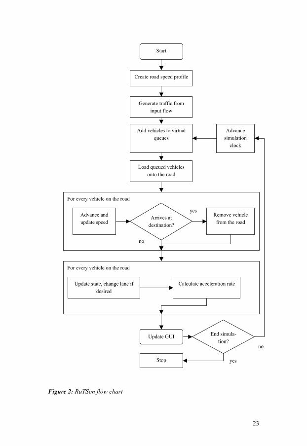
RuTSim uses a time-based scanning simulation approach. The simulation clock is advanced with a user defined step size, e.g. 0.1 second. The time-based simula-tion approach is chosen for RuTSim since it allows more detailed modeling of individual vehicle’s interactions with the surrounding traffic and the infrastruc-ture. With shorter time step, the movement of vehicles from one time step to the next becomes smoother and therefore more realistic. Hence, shorter time step may, given an adequate modeling logic, result in individual vehicle driving course of events closer to driving course of events found in real traffic. Shorter time step does however increase the model run time. The model time step should therefore be chosen in relation to the current application. Outputs in the form of aggregated traffic measures do not require as short time step as if representative vehicle driv-ing course of events is desired.

During a model run the following steps are performed in every time step:

22

1. Add vehicles that are to enter the road during the time step to virtual queues, one queue for each origin.

2. Load vehicles from virtual queues to the road if it is possible, i.e. if there is an acceptable space available on the main road.

3. For every vehicle on the road: Update speed and position. 4. Remove vehicles that have arrived to their destination. 5. For every vehicle on the road: Update state, i.e. free or car-following,

overtaking or passed, and acceleration rate. 6. Save data. 7. If animation is enabled, update the graphical user interface (GUI). 8. If the stop time has been reached; terminate the simulation, else; incre-

ment the simulation clock and go to step 1. The speed profile of the road and the traffic that is to enter the road are, prior to

the simulation, generated from the input road and traffic data respectively. A flow chart of the RuTSim model is included in Figure 2. The details of the modeling logic utilized in the different sub-models of RuTSim will be presented in the fol-lowing sections.

23

Figure 2: RuTSim flow chart

no

yes

Start

For every vehicle on the road

Advance and update speed

Remove vehicle from the road

Arrives at destination?

For every vehicle on the road

Calculate acceleration rate Update state, change lane if desired

Create road speed profile

Generate traffic from input flow

Add vehicles to virtual queues

Load queued vehicles onto the road

Update GUI End simula-tion?

Stop

Advance simulation

clock

no

yes

24

3.2 Road Representation This section presents the road representation utilized in RuTSim. Both the re-quired road data and the model’s representation of different types of rural roads will be described.

3.2.1 Road data RuTSim characterizes the road with variables defining the road geometry, the road section type and the traffic regulations along the road. The road representa-tion also includes the variables that are used to characterize intersections and roundabouts.

The road geometry is defined by the following variables: • Horizontal curvature • Vertical grade • Sight distance • Road width Values of the variables, horizontal curvature, vertical grade and road width are required for the beginning of the road and at every point along the road where the variable is changing. The value is assumed to be valid until the point where a new value is specified or until the end of the road. Sight distances must be specified in both directions of the road. To recreate representative overtaking behavior, the model requires the location and the sight distance for at least every sight maxi-mum and minimum along the road.

The road section type may be changing along the road. In similar fashion as the road geometry variables, the specified section type is assumed to be valid until a new section type is specified or until the end of the road. The section type must also be given at least at the start of the road in each direction. RuTSim handles the following road section types: • Normal two-lane highway with oncoming traffic • Two-lane highway including overtaking or climbing lane • One-lane section with a barrier between the oncoming lanes • Transient two-lane section with a barrier between the oncoming lanes that will

change into a one-lane section • Two-lane section with a barrier between the oncoming lanes and no indication

of change in the number of lanes Overtaking or climbing lanes are auxiliary lanes located to the right of the normal lane. These lanes are used by slow vehicles to let faster vehicles pass. The extra lane on two-lane sections is located to the left of the normal lane. This lane is used by vehicles to overtake slower vehicles in front. Transient two-lane sections com-bined with one-lane sections are used to model “2+1-roads” with the number of lanes in each direction changing between one and two at regular intervals.

The traffic regulations handled by the model are: • Overtaking restrictions • Speed limits

25

The model includes two types of overtaking restrictions, restrictions conveyed by road side signs and restrictions conveyed by barrier lines on the road. As the other variables presented above, both the overtaking restrictions and the speed limits must be specified at least in the beginning of the road in both directions of the road. The specified values are also assumed to be valid until a new value is speci-fied.

Intersections are characterized by the intersection location along the road, the secondary road entrances and the existence of dedicated left turn lanes on the main road. Regarding intersections, the model requires information on the exis-tence of an entrance from each side of the main road. This information determines if the intersection is three-way or four-way. For each existing intersection it is also necessary to specify if there is a stop or yield sign at the entrance of the secondary road. Moreover, the existence of left turn lanes must be specified for both direc-tions in connection with four-way intersections. For three-way intersections it is sufficient to specify the existence of left turn lanes in the direction where a left turn at the intersection is possible.

Roundabouts are characterized by the entrances from secondary roads and the radius to the centre of the roundabout carriageway. The secondary road entrances are specified in a similar fashion as the entrances to intersections. That is, the en-trances determine if the roundabout has three or four entrances.

3.2.2 Lanes and tracks A vehicle’s behavior may differ depending on which lane it currently travels in. For example, a vehicle traveling in the oncoming lane is likely to strive for a higher speed than in its normal lane. In similar fashion the speed is likely to be slower when traveling on the road shoulder. Due to such differences in driver be-havior it is necessary to keep track of the lane that each vehicle is in. To enable the possibility to keep track of different lanes, RuTSim divides the road carriage-way into a number of tracks according to Figure 3.

Figure 3: Track definition

That is, the oncoming lane or the left lane on two-lane sections is denoted track 1. The normal lane or the right lane on two-lane sections is denoted track 2. The road shoulder or the auxiliary climbing lane is denoted track 3. In connection with in-tersections incorporating a left turn lane the left turn lane is denoted track 4. This division of the road in different tracks allows RuTSim to assign different behavior to vehicles in different tracks or lanes.

The existence of road shoulders is determined using the road width data. The lane width is controlled by a model parameter. For two-lane roads, the road shoulder width is defined as the difference between half the road width and this lane width parameter. Vehicles are only able to use track 3 if the road shoulder

Direction 1 Direction 2

Track 3

Track 1

Track 2 Track 4

Track 3 Track 2

Track 1

26

width is greater than the minimum wide shoulder width. The minimum wide shoulder width is also a model parameter.

3.2.3 Sight distance function As presented in the section on required road data above, RuTSim requires sight distances in both directions of the road. From the given road coordinates and the matching sight distances, the model creates a piecewise linear sight distance func-tion for each direction of the road. This function is created by simple linear inter-polation between the road coordinates for which the sight distance is given in the input data. An example of a sight distance function is given in Figure 4.

Figure 4: Sight distance function

The sight distance function is used to approximate the sight distance at arbitrary points along the road. From the definition of the sight distance function it is clear that the more given sight distance measurements the more accurate sight distance approximation.

3.2.4 Speed profile The road representation of RuTSim also includes the speed profile of the road. The speed profile is used to determine the speed which vehicles strive for along the road. A distinct speed profile is constructed for each direction of the main road.

Each vehicle in the simulation is assigned a basic desired speed, 0iv . The basic desired speed is the speed a free driving vehicle would adopt on a straight road that is wide enough for the road width not to impose any restriction on the desired speed. These basic desired speeds are distributed according to vehicle type de-pendent normal distributions. The speed profile model modifies these basic de-sired speed distributions to the distributions of the actual speeds the vehicles will strive for taking in to account the road geometry and the speed limit.

The basic desired speeds of free driving cars on straight wide roads are as-sumed to be distributed according to a distribution with median speed 0v , where

0v is a model parameter. This speed is reduced with respect to the road width (i), the horizontal curvature (ii) and the speed limit (iii) to a new median speed 3v . This reduction will be described in detail below. The distribution dispersion

Road coordinate

Sight distances given in the input data

Sigh

t dis

tanc

e

27

around 3v is also modified with respect to the road geometry and the speed limit. The change of the distribution dispersion is characterized by a dispersion measure Q . The details of the calculation of Q are also presented below.

Given Q and the basic desired speed of an arbitrary vehicle, 0iv , the desired speed with respect to the road geometry and the speed limit, 3iv , is for cars ob-tained through the expression

0 3 0 3

Q Q Q Qi iv v v v− = − (3.1)

and for other vehicles as

0 3 0 3(1 )( ) .Q Q Q Q

i i iv v v vλ− − = − (3.2) The parameter iλ is a vehicle type dependent model parameter in the interval 0 1iλ≤ ≤ . Equation (3.2) is obtained by recognizing that the desired speed of cars varies more than the desired speeds of other vehicle types. This is a natural as-sumption for heavy vehicles since heavy vehicles due to their lower speeds are less sensitive to changes in, for example, speed limit. The parameter 0v and there-fore also the resulting speed 3v , are median speeds of free cars. Equation (3.2) is accordingly used to relate the median speeds of cars to the speeds of other vehicle types.

At all points where the road geometry changes or a new speed limit comes into effect the speed profile model gives a new median speed, 3v , and the correspond-ing dispersion measure Q .

Speed reduction with respect to the road width The median basic desired speed for cars on a straight wide road without speed limit, 0v , is reduced with respect to the road geometry and the speed limit to a desired speed for an arbitrary position along the road.

For roads narrower than 8 m, 0v is reduced to 81 1

mv v= , where 81

mv is a model parameter. For roads narrower than 7.5 m the speed 1v is further reduced via the expression:

1

81

1 ,12.5 5m

v a av w

=+ −

−

(3.3)

where w is the road width expressed in meters and a is a model parameter. Figure 5 depicts this expression for different values of the parameter a . As can be seen in the figure, the model becomes increasingly sensitive to narrow roads with in-creasing value on the parameter a .

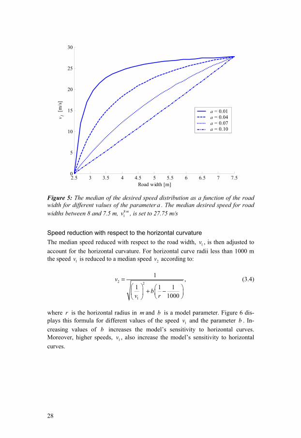
28

2.5 3 3.5 4 4.5 5 5.5 6 6.5 7 7.50

5

10

15

20

25

30

Road width [m]

v1 [

m/s]

a = 0.01 a = 0.04 a = 0.07 a = 0.10

Figure 5: The median of the desired speed distribution as a function of the road width for different values of the parameter a . The median desired speed for road widths between 8 and 7.5 m, 8

1mv , is set to 27.75 m/s

Speed reduction with respect to the horizontal curvature The median speed reduced with respect to the road width, 1v , is then adjusted to account for the horizontal curvature. For horizontal curve radii less than 1000 m the speed 1v is reduced to a median speed 2v according to:

2 2

1

1 ,1 1 1

1000

v

bv r

= + −

(3.4)

where r is the horizontal radius in m and b is a model parameter. Figure 6 dis-plays this formula for different values of the speed 1v and the parameter b . In-creasing values of b increases the model’s sensitivity to horizontal curves. Moreover, higher speeds, 1v , also increase the model’s sensitivity to horizontal curves.

29

10

20

30 v1 = 20 [m/s] b = 0.1 b = 0.15 b = 0.2 b = 0.25

10

20

30

v2 [

m/s]

v1 = 25 [m/s]

0 100 200 300 400 500 600 700 800 900 1000

10

20

30

Horizontal radius [m]

v1 = 30 [m/s]

Figure 6: The median of the desired speed distribution as a function of the hori-zontal radius for different values of the parameter b . The sub-figures display the relationship for different speeds 1v

Speed reduction with respect to the speed limit The speed reduction process is completed with the reduction of the median speed

2v with respect to the speed limit to the final median desired speed, 3v . The speed

3v is obtained as:

( )2

2

23

3.6

,

1limit

limit

vv

vv

c v d

=

+

(3.5)

where limitv is the current speed limit in km/h, d is a model parameter and

( )limitc v is a function of the speed limit defined in the following way:

( ) 1.30 0.015 90 .limit limitc v v= − ⋅ − (3.6) Figure 7 depicts the relationship between the desired speed, 3v , and the speed

limit for different values of the parameter d and the speed 2v . As can be seen in the figure the speed limit has less impact when the speed 2v is low. This is an in-tuitive feature since vehicles are already constrained by the road width and/or the horizontal curvature when the speed 2v is low. For low speed limits the desired

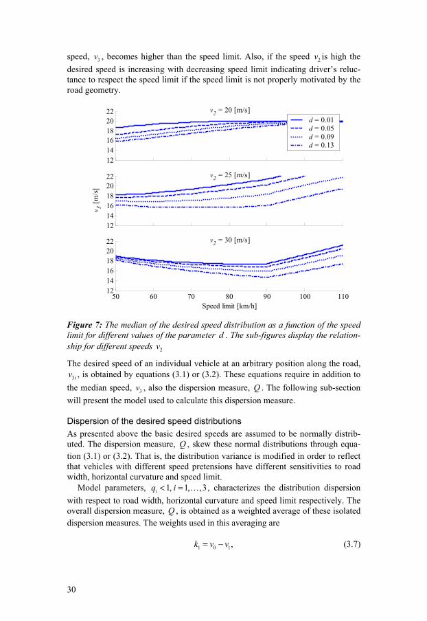
30

speed, 3v , becomes higher than the speed limit. Also, if the speed 2v is high the desired speed is increasing with decreasing speed limit indicating driver’s reluc-tance to respect the speed limit if the speed limit is not properly motivated by the road geometry.

121416182022 v2 = 20 [m/s]

d = 0.01 d = 0.05 d = 0.09 d = 0.13

121416182022

v3 [m

/s]

v2 = 25 [m/s]

50 60 70 80 90 100 110121416182022

Speed limit [km/h]

v2 = 30 [m/s]

Figure 7: The median of the desired speed distribution as a function of the speed limit for different values of the parameter d . The sub-figures display the relation-ship for different speeds 2v

The desired speed of an individual vehicle at an arbitrary position along the road, 3iv , is obtained by equations (3.1) or (3.2). These equations require in addition to

the median speed, 3v , also the dispersion measure, Q . The following sub-section will present the model used to calculate this dispersion measure.

Dispersion of the desired speed distributions As presented above the basic desired speeds are assumed to be normally distrib-uted. The dispersion measure, Q , skew these normal distributions through equa-tion (3.1) or (3.2). That is, the distribution variance is modified in order to reflect that vehicles with different speed pretensions have different sensitivities to road width, horizontal curvature and speed limit.

Model parameters, 1, 1, ,3iq i< = … , characterizes the distribution dispersion with respect to road width, horizontal curvature and speed limit respectively. The overall dispersion measure, Q , is obtained as a weighted average of these isolated dispersion measures. The weights used in this averaging are

1 0 1,k v v= − (3.7)

31

( )2 1 22k v v= − (3.8) and

( )3 2 32.5 ,k v v= − (3.9) for 1q , 2q and 3q respectively, 0 1 2 3, , andv v v v are the median of the basic desired speed distribution and the reduced median speeds obtained from equations (3.3)-(3.5) above. The dispersion measure Q is formed as

1 1 2 2 3 3

1 2 3

.q k q k q kQk k k+ +=+ +

(3.10)

If 0, 1, ,3ik i= = … then 1Q = by definition.

The relative size of the weights (3.7) - (3.9) implies that horizontal curvature has greater impact than road width and speed limit has greater impact than hori-zontal curvature on the dispersion measure Q . Since 1, 1, ,3iq i< = … the overall dispersion measure Q also satisfy 1Q < . This implies that vehicles with high ba-sic desired speeds will reduce their speeds more than vehicles with lower basic desired speeds.

Figure 8 displays the result of the complete speed profile model for a 9 m wide road with horizontal radius 400 m. The figure contains the resulting desired speed distributions for different vehicle types. The speed limit is 90 km/h and the basic desired speeds were assumed to be distributed according to

(30.25 ,3.2 )N m s m s , (26.5,2.9)N and (24.3,1.5)N for cars, trucks (and bus-ses) and trucks with trailer respectively. The parameters used to produce the figure were 0.042a = , 015b = , 0.5, 0.8, 2iq = − − for 1, 2, 3i = respectively and

0.3iλ = and 0.5 for trucks and trucks with trailer respectively. The graphs show that the speed profile model modifies the speed distribution of cars more than the speed distributions of other vehicle types. This is a direct consequence of the pa-rameters iλ in equation (3.2). As described above these parameters are used to model that cars are more sensitive to different road alignment than heavy vehicles. The effect of the distribution dispersion measure, Q , is also visible in the graphs. In this example 1.47Q = − indicates that the speed of faster vehicles will be re-duced more than the speed of slower vehicles. This effect is clearly visible in the cumulative distribution functions sub-figure where the curves are shifted more towards lower speed for high speed percentiles than for low speed percentiles.

32

0

0.1

0.2

Probability density functions

v0 carsv3 carsv0 trucks & bussesv3 trucks & bussesv0 trucks with trailerv3 trucks with trailer

10 15 20 25 30 35 400

0.2

0.4

0.6

0.8

1 Cumulative distribution functions

Speed [m/s]

Figure 8: Basic desired speed distributions and the resulting desired speed distri-butions

Preparation for upcoming change in desired speed At all points where the road width or the horizontal curvature changes or a new speed limit comes into effect, a new median speed, 3v , and the corresponding dis-persion measure, Q , are calculated by the speed profile model.

When approaching an obstacle such as a curve, or if the road becomes nar-rower, most drivers start to decelerate before they reach the obstacle. RuTSim incorporates such behavior by moving the points where a new desired speed comes into effect. That is, all points of change in desired speed are moved back with respect to the direction of travel by a distance, L , given by

2 23 3

3 3

3 3

( ) ( ) ,2

0, ,

previous nextprevious next

normalprevious next

v v v vL a

v v

− >= ≤

(3.11)

where normala is a deceleration rate corresponding to the median vehicle’s engine deceleration. 3

previousv and 3nextv are the previous and next median desired speeds,

respectively. The effect of equation (3.11) is that vehicles adjust their speeds be-fore reaching obstacles. On the other hand, vehicles do not start to accelerate be-fore profitable changes have come into effect, i.e. when 3 3

previous nextv v≤ .

33

Desired speed in roundabouts and intersections The speed profile model is also used to calculate the distribution of desired turn speeds for different turn movements at intersections and roundabouts along the main road. For both roundabouts and turns at intersections the distributions of desired turn speeds are calculated in the same way as the distributions of desired speeds for road sections presented above.

For intersections the road width used in equation (3.3) is the width of the main road at the intersection. The horizontal radius in equation (3.4) is, for left turns, approximated with the main road width. For right turns, half the main road width is used to approximate the horizontal radius. Finally, the speed limit used in equa-tion (3.5) is the speed limit on the main road at the intersection.

The road width used in the calculation of the distributions of desired speeds in roundabouts is taken as the standard lane width times the number of lanes, where the standard lane width is a model parameter. The horizontal radius of a round-about is the roundabout radius specified in the input data.

Figure 9 shows the median of the desired speed distribution for cars, i.e. 3v , as a function of the turn curve radius. The parameters used to construct this figure are identical to the parameters used in Figure 8. That is, the graph is valid for a 9 m wide main road with speed limit 90 km/h. The graph shows that the median of the desired turn speed distribution for cars will be about 7.8 m/s for left turns and about 5.5 m/s for right turns. In similar fashion, the median desired speed for cars in a roundabout with radius 25 m and carriageway width 9 m is according to the graph 12 m/s.

0 5 10 15 20 25 30 35 40 45 500

2

4

6

8

10

12

14

16

Med

ian

desir

ed tu

rn sp

eed

[m/s]

Turn curve radius [m]

Figure 9: Desired turn speed for the median car as a function of the turn curve radius

34

3.3 Traffic Generation This section presents the traffic generation model of RuTSim. The traffic that is to enter the road during the simulation run is generated prior to the simulation. This generation process creates individual vehicles and determines the created vehi-cles’ entry times and speeds.

3.3.1 Traffic data The traffic flows that are to enter from each origin in each direction of road must be specified prior to a simulation run. Each main road entrance from secondary roads at every intersection and roundabout is considered to be a possible origin. Both ends of the simulated road are also possible origins.

The traffic volume in vehicles per hour and the composition of different vehi-cle types must be specified for each flow. The start time and the duration of the flow must also be specified. There may be several flows from each origin during a simulation run, i.e. the traffic volume and composition may vary during the simu-lation. Overlapping flows from a specific origin is however not allowed.

For each origin with non-zero flow the proportion of vehicles exiting at differ-ent destinations is also required. The ends of the main road and each intersection or roundabout are possible destinations. Turning proportions must also be speci-fied if the destination is located at an intersection or in a roundabout. The above described traffic data hierarchy is displayed in Figure 10.

Figure 10: Hierarchy of traffic data

Traffic data

Direction 1 Direction 2

Origins

Origin 1 Origin n

Location Flows Destinations

Flow 1 Flow n

Destination 1 Destination n

End time

Com-position

Start time

Volume

Location Turn percentages

…

…

…

35

3.3.2 Vehicle characteristics Vehicles are defined by the individual vehicle characteristics. The vehicle charac-teristics can be divided into static vehicle properties that remain constant during the simulation and dynamic vehicle properties that change as the vehicle travels along the road during the simulation.

The static vehicle properties are, with index i referring to vehicle i :

• Vehicle type, iτ • Length, il [ ]m • Power to mass ratio (p-value), ip [ / ]W kg • Basic desired speed, bds

iv 2[ / ]m s • Origin, iO • Destination, iD • Entry time, entry

it [ ]s • Desired following time gap, iT [ ]s • Reaction time, react

it [ ]s • Air resistance coefficient, A

iC 1[ ]m− • Rolling resistance coefficients, 1R

iC 2[ / ]m s and 2RiC 1[ ]s−

All static vehicle properties are set in the traffic generation process. The traffic generation model includes four vehicle types, iτ : car, truck and buss, truck with trailer and truck with semi-trailer. The p-value, ip , is the power to mass ratio measured at the wheels, ip controls the acceleration ability of the vehicle. For heavy vehicles, the p-value corresponds to the maximum power available. For cars, the p-value reflects the power used in normal acceleration situations. The basic desired speed, bds

iv , is the individual basic desired speed described in section 3.2.4 above. The origin, iO , and destination, iD , includes the road coordinate of the entrance or destination point respectively. The main road entry and exit side is also included in the origin and destination respectively. If the origin or destination is at an intersection or a roundabout the main road entry or exit side may be either left or right. For vehicles with origin or destination at the ends of the main road the entrance or exit is at the centre of the road. The entry time, entry

it , is the first time that the vehicle will try to enter the main road. The reaction time, react

it , is the time between changes in behavior in connection with car-following.

The dynamic vehicle properties include:

• Position, ix [ ]m • Track, iψ • Speed, iv [ / ]m s • Acceleration, ia 2[ / ]m s • Desired speed, des

iv [ / ]m s

36

The position, ix , is the coordinate of the vehicle’s current position on the road. The track, iψ , is the current track of the vehicle, see section 3.2.2 above. The speed, iv , and acceleration, ia , is the current speed and acceleration of the vehi-cle. Finally, the desired speed, des

iv , is the individual vehicle desired speed given by the speed profile model, i.e. des

iv is denoted 3iv in section 3.2.4 above. 3.3.3 Platoon generation RuTSim utilizes a platoon generation model to reduce the simulation warm-up time required before stable traffic conditions are formed. This model creates pla-toons of vehicles representative for the current traffic composition and volume. The platoons are characterized by the number of platoon vehicles and the head-way for the platoon leader to the last vehicle of the previous platoon.

The platoon generation procedure works as follows: The average platoon length is estimated for every flow from every origin in each direction of the road. A series of free and constrained vehicles corresponding to this average platoon length is then created using uniformly distributed random numbers. Platoon lead-ers and platoon vehicles are then assigned entry times drawn from the headway distribution for free and platoon vehicles respectively.

The average platoon length, µ̂ , given current traffic conditions is obtained through the following expressions (Miller, 1967):

0.58 1.58 , 1

ˆ1 1.16 , 1,

Z ZZ Z

µ+ ⋅ >

= + ⋅ ≤ (3.12)

where Z is given by

0.1 , 0

20, 0,

fqZ λ

λλ

⋅ >=

≤

and fq is the traffic volume in the current direction in vehicles per hour and λ is a measure of the current overtaking possibility . The parameter λ is obtained as

( )0.66 1 ln 2 ,3600

f co hv

q tA q pλ −

= ⋅ − −

(3.13)

where A is a road standard parameter, oq is an estimate of the flow in the opposite direction, ct is the average time gap between constrained vehicles for the current traffic composition and hvp is the proportion of heavy vehicles in the current flow. The parameters A and ct are model parameters. All other variables are de-rived from the input data. For origins located at secondary road entrances the flow in the opposite direction, oq , should equal the flow exiting the main road to the secondary road. Since vehicles are not only considering the conditions on the sec-ondary road when entering, but also the gap in the main road traffic the platooning

37

of secondary road vehicles is considered less important. As a consequence, in connection with origins located at secondary road entrances, the flow oq is ap-proximated with fq .

Given µ̂ , the estimated proportion of free vehicles is ˆ1 µ , i.e. one vehicle per platoon (the platoon leader) is free, and the proportion of car-following platoon vehicles is ˆ1 1 µ− . A series of free and car-following vehicles are created using uniformly distributed random variables, [ ]0,1X U∼ . A drawn value ˆ1x µ< re-sults in a free vehicle being created, i.e. a platoon leader, and if ˆ1x µ≥ a con-strained car-following vehicle is created. Successive free vehicles are allowed, i.e. platoons of one vehicle are allowed. The number of vehicles that are to be created is obtained as the duration of the current flow times the traffic volume, fq .

Due to the use of random numbers the average length of the created platoons may differ slightly from µ̂ . Denote this generated mean platoon length by genµ . With a flow of q vehicles per hour the time, in seconds, of the mean platoon can be obtained as 3600 /genµ q . This time can also be expressed as the sum of the time gap for the platoon leader and 1genµ − time gaps for the platoon vehicles, that is

3600

( 1) .genf gen c

µt µ t

q= + − (3.14)

where ft is the mean time gap for free vehicles and ct is defined in connection with equation (3.13) above. Equation (3.14) is approximate since the time occu-pied by the vehicles of the platoon has been neglected. The approximation is for this reason more accurate the smaller the proportion of long vehicle types in the current flow.

The time gaps between platoons, i.e. the time gap for free vehicles, are as-sumed to be exponentially distributed with mean f mint d− , where mind is the minimum time gap for free vehicles. The parameter ft is obtained from equation (3.14) and the distribution of free vehicles time gaps ( )h t is given by

,( )

0, .

min

f min

t dt d

minf min

min

e t dh t t d

t d

−−−

≥= − <

(3.15)

Constrained platoon vehicles time gap to the vehicle in front is assumed to be

distributed according to vehicle type dependent lognormal distributions with mean values ct

τ and variances 2τσ . These distribution parameters, ct

τ and 2τσ , are vehi-

cle type dependent model parameters. The average time gap between platoon ve-hicles, ct , is obtained as a weighted average of these vehicle type dependent time gaps. The weights are chosen to correspond to the vehicle type composition of the current flow.

38

Denote the distributions of constrained platoon vehicles time gaps with ( )g tτ where τ denotes vehicle type. With vehicle type proportions

ipτ in the current

flow, the composite time gap frequency function of the current flow, ( )f t , be-comes

( ) ( ) ( )1 11 .ii

gen gen if t h t p g tτ

τµ µ

= + − ∑ (3.16)

Figure 11 depicts the composite time gap probability density function for

symmetric traffic flows of 300 vehicles per hour in each direction on a road with standard 3000A = . The heavy vehicle percentage of the flows is 15 %. The esti-mated average platoon length is 1.98 vehicles and the average time gaps for free and platoon vehicles are 21.76 and 2.06 seconds respectively.

0 10 20 30 40 50 60 70 80 900

0.005

0.01

0.015

0.02

0.025

0.03

0.035

0.04

0.045

Time gap [s]

Figure 11: Time gap probability density function for symmetric flows, 300 vehi-cles/h, and road standard 3000. The heavy vehicle percentage of the flows is 15 %

Each vehicle in the generated platoons is assigned an entry time taken as the entry time of the previous vehicle and an inter-entry time. The inter-entry times are cal-culated as vehicle length divided by entry speed for the previous vehicle and a time gap drawn from the appropriate distribution depending on whether the vehi-cle is a platoon leader or a constrained vehicle. The model for vehicle entry speeds will be presented in the next section. For platoon vehicles the time gap is also set as the vehicle’s desired following time gap, iT . Free vehicles are also assigned desired following time gaps from the lognormal constrained vehicle time gap dis-tribution corresponding to the type of the free vehicles.

39

The platoon generation process described above is repeated for every flow and every origin in each direction. 3.3.4 Generation of vehicle characteristics As mentioned in the previous section, free and car-following platoon vehicles are created in the platoon generation model. The platoon generation model determines vehicle entry times. The remaining vehicle properties described above are how-ever also set in the vehicle generation process.

Vehicles are randomly assigned type according to the traffic composition of the current flow. The vehicle length is then drawn from the distribution of vehicle lengths for the previously assigned vehicle type. Vehicles are in similar fashion assigned reaction times drawn from vehicle type specific distributions. Both the vehicle lengths and the reaction times are assumed to be normally distributed. The reaction time is modified to the number of complete time steps closets to the drawn value. The air and rolling resistance coefficients of the vehicle are set to standard values for the current vehicle type.

The vehicles are randomly assigned destinations according to the turning pro-portions of the flow that the vehicle belongs to. The origin property of the vehi-cles is simply set to the origin of the flow.

The basic desired speed and p-value properties of the vehicles are also set at vehicle creation. These properties are coupled in order to make sure that it is pos-sible for each vehicle to maintain its desired speed in level terrain. The basic de-sired speed is drawn from a vehicle type specific normal distribution. The basic desired speed distributions are truncated at 2.5± standard deviations in order to avoid extremely fast or slow vehicles. The p-value is then drawn from vehicle type specific normal distributions with the following constraint imposed on the drawn p-value, ip :

( ) ( )1 2

3 2.bds bds bds

i A i R i R ip C v C v C v≥ + + (3.17) The notation introduced in section 3.3.2 above is used in the constraint above. The effect of the p-value constraint in equation (3.17) is that vehicles will not be as-signed p-values that are too small for the vehicles to attain their desired speed in level terrain.

After vehicles are given basic desired speeds and p-values, vehicles are per-muted within their respective platoons. This permutation is done in order to make sure that it is the slowest vehicle that is the platoon leader. Platoons should not split up unless overtakings are performed or if slow vehicles exit the road. The permutation is performed as follows. For every platoon the vehicle with the low-est basic desired speed is identified. This vehicle and the platoon leader then switch position in the platoon. By this procedure the slowest vehicle becomes the platoon leader. The entry times of the vehicles are also changed in the switching process. Not only is the arrival times of the vehicles that are actually switched changed. Since the arrival times of the vehicles depend on properties of the pre-ceding vehicles, the vehicles following the vehicles that change place are also influenced by the switching. Therefore, the entry times of these vehicles are modi-fied to the appropriate values given their new leaders.

40

Platoon leaders are assigned entry speeds equal to the vehicles’ individual de-sired speed at the location of the origin. This desired speed is given by the speed profile model as described in section 3.2.4. That is, if the origin is located at an intersection or in a roundabout the entry speed will be equal to the desired turn speed for the entry turn movement. Similarly, if the origin is located at one of the ends of the simulated road the entry speeds will be equal to the vehicles’ desired speeds with respect to the road geometry and cross-section at the location of the origin.

Constrained platoon vehicles are assigned entry speeds equal to the speed of the preceding vehicle. This implies that platoon vehicles are not required to adjust their speeds with respect to their leader immediately upon entry.

3.4 Vehicle Movements This section presents the vehicle movement logic of RuTSim. This includes the loading and unloading of vehicles on the road and the movement of individual vehicles as they travel along the road during simulation runs.

3.4.1 Acceleration model In RuTSim a vehicle’s speed is controlled by adjusting the vehicle’s acceleration rate. The acceleration model of RuTSim is divided into two main sub-models; a model for speed adaptation with respect to the road geometry and a model for speed adaptation in connection with car-following.

The notation introduced in section 3.3.2 will be used in the following descrip-tion of the acceleration model. Index n will be used to denote the current vehicle and index 1n − represents the vehicle in front of the current vehicle. The utilized notation is displayed in Figure 12 below.

Figure 12: Vehicle movement notation

The position of vehicle n is denoted nx and nv and na are used to denote the speed and acceleration respectively. The length of vehicle n is represented by nl . State qualification The state qualification process determines which of the acceleration sub-models that should determine the acceleration rate. Vehicles are classified as free or car-

n n-1

,n nv a 1 1,n nv a− −

nl 1nl −

nx

1nx −

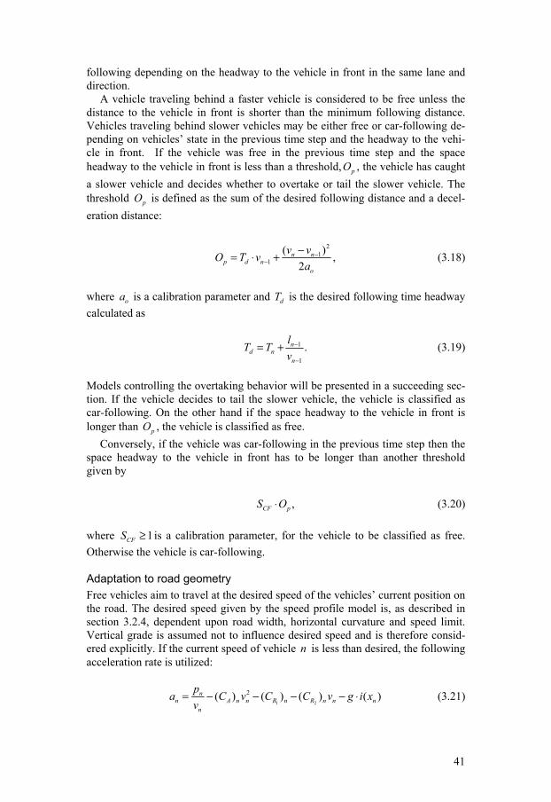
41

following depending on the headway to the vehicle in front in the same lane and direction.

A vehicle traveling behind a faster vehicle is considered to be free unless the distance to the vehicle in front is shorter than the minimum following distance. Vehicles traveling behind slower vehicles may be either free or car-following de-pending on vehicles’ state in the previous time step and the headway to the vehi-cle in front. If the vehicle was free in the previous time step and the space headway to the vehicle in front is less than a threshold, pO , the vehicle has caught a slower vehicle and decides whether to overtake or tail the slower vehicle. The threshold pO is defined as the sum of the desired following distance and a decel-eration distance:

2

11

( ) ,2

n np d n

o

v vO T va

−−

−= ⋅ + (3.18)

where oa is a calibration parameter and dT is the desired following time headway calculated as

1

1

.nd n

n

lT Tv

−

−

= + (3.19)

Models controlling the overtaking behavior will be presented in a succeeding sec-tion. If the vehicle decides to tail the slower vehicle, the vehicle is classified as car-following. On the other hand if the space headway to the vehicle in front is longer than pO , the vehicle is classified as free.

Conversely, if the vehicle was car-following in the previous time step then the space headway to the vehicle in front has to be longer than another threshold given by

,CF pS O⋅ (3.20) where 1CFS ≥ is a calibration parameter, for the vehicle to be classified as free. Otherwise the vehicle is car-following. Adaptation to road geometry Free vehicles aim to travel at the desired speed of the vehicles’ current position on the road. The desired speed given by the speed profile model is, as described in section 3.2.4, dependent upon road width, horizontal curvature and speed limit. Vertical grade is assumed not to influence desired speed and is therefore consid-ered explicitly. If the current speed of vehicle n is less than desired, the following acceleration rate is utilized:

1 2

2( ) ( ) ( ) ( )nn A n n R n R n n n

n

pa C v C C v g i xv

= − − − − ⋅ (3.21)

42

The function ( )ni x represents the vertical grade at the position of vehicle n . The parameter g is the acceleration due to gravity. The first term of the right hand side of equation (3.21) represents the maximum possible acceleration of vehicle n given the vehicle’s current speed. The remaining terms reduces this maximum acceleration by the air and rolling resistances and the acceleration due to gravity.

If the current speed of vehicle n is higher than desired, the utilized decelera-tion rate is given by

1 2

1 2

2

2

( ) ( ) ( ) ( ), ( ) 0

( ) ( ) ( ) , ( ) 0,A n n R n R n n n n

nA n n R n R n n n

C v C C v g i x i xa

C v C C v i x

− − − − ⋅ ≥= − − − <

(3.22)

with the same notation as in equation (3.21). That is, vehicles are assumed to re-duce their speed on level terrain and uphill, i.e. ( ) 0ni x ≥ , through engine decel-

eration and downhill, i.e. ( ) 0ni x < , by the use of the decelerator pedal. The decelerator pedal is assumed to be used to balance the acceleration due to gravity. Car-following Car-following vehicles strive to follow the vehicle in front at a distance corre-sponding to the time gap given by equation (3.19). When a vehicle catches a slower vehicle and decides to follow, the vehicle decelerates to obtain the speed of the vehicle in front at the desired following distance. In similar fashion, if the leader accelerates then the follower accelerates to catch up with the leader. The acceleration rate is in these situations, when the distance to the vehicle in front is longer than desired, given by

2 2

1

1

,2( )

n nn

d n

v vaT v

−

−

−=⋅

(3.23)

where dT is defined as in equation (3.19). Vehicles acceleration resources are lim-ited and individual. If the acceleration rate given by equation (3.23) is larger then the acceleration rate prescribed by equation (3.21) it is neither desirable nor pos-sible for the follower to adopt the acceleration rate of equation (3.23). In such cases the follower’s acceleration rate is dictated by equation (3.21) even though it is at present in the car-following state.

If the distance to the leader becomes shorter than desired and the speed of the follower is higher than or equal to the speed of the leader, the follower must de-celerate to extend the distance to the leader. The adopted deceleration rate is an interpolation between the follower’s engine and maximum deceleration rates,

enginend and max

nd . That is, the deceleration rate used to extend the distance to the leader may be expressed as:

43

1 1

1

( ) ,

, ,

max engineenginen n

n n min nmin n

nmaxn min

d d T T d T T TT T

ad T T

− −−

− − + ≤ ≤ −= <

(3.24)

where T is the current time gap to the leader and minT is a time gap threshold. The time gap threshold and the engine and maximum deceleration rates are all calibra-tion parameters.

Vehicles’ change of deceleration rate is not immediate in the car-following state. Instead the acceleration rate of a car-following vehicle is updated with a frequency of 1 react

nt . The result of this procedure is a lag in the response to leader actions. However, the acceleration rate is immediately adjusted according to equa-tion (3.23) when vehicles catch slower vehicles. Also, if a vehicle changes lane in front of a car-following vehicle the car-following vehicle will immediately adjust its speed to the new situation. Such situations occur for example when overtakings are completed and the overtaking vehicle returns to the normal track. Similarly if the leader exits the road at an intersection, the follower will become free and im-mediately change its acceleration.

Constraining vehicle Normally the vehicle that prevents a vehicle from attaining its desired speed is the vehicle in front in the same track or a vehicle in a track to the left of the vehicle. As a consequence, car-following vehicles follow the vehicle in the same track or a track to the left for which the time to collision is shortest. The time to collision,

colt , is estimated by:

1 1

11

1

,

, ,

n n nn n

n ncol

n n

x l x v vv vt

v v

− −−

−

−

− − > −= ∞ ≤

(3.25)

where 1nv − is the constraining vehicle candidate and nv is the car-following vehi-cle.

However, in connection with lane drops and at the beginning of overtaking re-strictions, i.e. at track endings, it is necessary to alter this following priority. In connection with such situations a merging area is defined by a model parameter, ξ . Figure 13 below depicts a merging situation in connection with a lane drop.

44

Figure 13: Lane drop merging situation

No overtakings are permitted within the merging area, i.e. the vehicles will merge in the order they enter the merging area. As a consequence the constraining vehi-cle will be the vehicle in front closest to the vehicle regardless of the track of the vehicle in front. Vehicles traveling in a track that ends will, if the time to the track ending is longer than colt , use the car-following acceleration rate given by equa-tion (3.23) or (3.24). On the other hand, if the time to the track ending is shorter than colt , the vehicle will adopt the acceleration rate needed to stop at the track ending:

,2

nn track

n

vas−= (3.26)

where track

ns is the distance left to the track ending as defined in Figure 13. The time to the track ending is obtained as track

n ns v . 3.4.2 Overtaking model The purpose of the overtaking model is to control the situations when vehicles are given opportunities to overtake and the vehicles’ behavior when overtaking. The overtaking behavior on normal two-lane highways differs from the overtaking behavior on rural roads with a barrier between the oncoming traffic lanes. As a consequence, RuTSim separates the overtaking behavior on these road types.

Two-lane sections with oncoming traffic RuTSim includes two types of overtakings on two-lane roads with oncoming traf-fic; flying and accelerated overtakings. Flying overtakings are overtakings in con-junction with vehicles catching slower vehicles and instantly decides to overtake. Accelerated overtakings are all other overtakings where the vehicles with higher speed pretensions tail slower vehicles and have to accelerate to overtake their leaders.

When a vehicle catches a slower vehicle it receives an opportunity for a flying overtaking at the catching up point pO defined in equation (3.18). A tailing vehicle receives opportunities for accelerated overtakings at positions along the road

ξ

1n −

n trackns

45

where the sight distance attains a maximum. Moreover, if an overtaking opportu-nity is declined due to an oncoming vehicle within sight then the tailing vehicle will receive a new overtaking opportunity when the oncoming vehicle has passed. If the vehicle to overtake is part of a platoon, the overtaking vehicle is given an opportunity for multiple overtakings when it is side-by-side with the vehicle to overtake. Multiple overtakings are treated as flying overtakings.

The overtaking decision process is governed by four conditions: 1. The vehicles’ ability to overtake 2. The possibility to overtake considering the surrounding traffic 3. Possible overtaking restrictions 4. The drivers’ willingness to overtake

The appraisal of a vehicle’s ability to overtake is divided into two parts. First the estimated overtaking distance must be smaller than the maximum allowed over-taking length, max

ovtkl . Secondly, in connection with accelerated overtakings, the dif-ference in desired speed between overtaking and overtaken vehicles must be above the minimum allowed desired speed difference, min

ovtkv∆ . In connection with flying overtakings the estimated overtaking distance is given by

1

1

,rel novtk rel

n n

l vl lv v

−

−

= +−

(3.27)

where rell is the distance which the overtaking vehicle must travel relative to the vehicle to be overtaken. This relative distance is given by:

1 .rel n n n n nl x x l T v−= − + +

In case of accelerated overtakes the overtaking distance is estimated as

2 ,relovtk relmax

n

ll la

= + (3.28)

where max

na is the overtaking vehicles maximum acceleration given its current position and speed. This maximum acceleration is given by equation (3.21).

The condition regarding the possibility to overtake considering the surrounding traffic assures that it is possible to initiate an overtaking with respect to the traffic in the overtaking vehicles own direction. That is, the overtaking track must be vacant both in front and behind the overtaking vehicle. A vehicle is not allowed to commence an overtaking if it is being overtaken. Moreover, as vehicles are not allowed to travel too close to each other, the overtaking track must be free a cer-tain distance in front of the vehicle. This distance is the distance corresponding to the overtaking vehicle’s desired following time headway, nT . In addition, overtak-ings are not allowed if any vehicle in the platoon ahead is preparing to make a left turn at an upcoming intersection. That is, if any vehicle ahead has started to slow down in order to exit the main road by a left turn.

46

Vehicles are not allowed to initiate overtakings if there is any type of overtak-ing restriction at the vehicles position on the road nor if there is any overtaking restriction within the minimum distance to overtaking restrictions, rest

ovtkl . The same holds if there is a climbing or overtaking lane within rest

ovtkl . If so, the vehicles await the auxiliary lane for the overtaking.

Finally, the driver must be willing to accept the overtaking with the current sight distance or the current distance to an oncoming vehicle taken into considera-tion. RuTSim uses a collection of Gompertz functions to describe driver’s will-ingness to overtake slower traffic. The functions are of the form:

/

min/

min

exp( exp( )),[ ]

0, ,

flying acc

flying acc

A ks s sP s

s s − − >

= ≤ (3.29)

where [ ]P s is the overtaking probability given a clear sight distance s . The threshold /

minflying accs is the minimum clear sight distance for flying or accelerated

overtaking. These functions are estimated from empirical data. Distinct functions are estimated for different, road widths, types of overtaking, overtaken vehicle and sight limiting factor, i.e. natural obstacles or oncoming vehicles. That is, dif-ferent parameters A and k are given for each combination of the following at-tributes:

• Type of overtaking o Flying o Accelerated

• Sight limitation o Oncoming vehicle o Natural obstacle

• Overtaken vehicle o Car traveling at speed below 90 km/h o Car traveling at speed over 90 km/h o Truck o Truck with trailer or semi-trailer

• Road width o Roads with paved shoulders, i.e. road widths over 11 m o All roads narrower than 11 m

For a complete description of the overtaking probability functions see Carlsson (1990) and (1991). The utilized parameters A and k are also included in Appen-dix A.

In connection with flying overtakings, the overtaking probability of equation (3.29) is reduced according to the following expression if the vehicle ahead is part of a platoon:

1[ ] [ ],red NP s P sη −= ⋅ (3.30)

47

where N is the number of vehicles in the platoon ahead and η is a parameter con-trolling the reduction per vehicle in the platoon. However, no reduction of the overtaking probability is done in connection with multiple overtakings.

Vehicle platoons are discharged in order of priority from the front of the pla-toon. As a consequence, only the vehicle behind the platoon leader is allowed to perform an accelerated overtaking. If the second vehicle in the platoon rejects an opportunity for an accelerated overtaking no other vehicle in the platoon will re-ceive an overtaking opportunity.

If an overtaking is accepted, the overtaking vehicle changes track to the on-coming traffic’s lane, i.e. track 1 in Figure 3 is used. When traveling in the on-coming traffic’s lane the vehicle’s desired speed, des

nv , is incremented by a factor desovtkv . As a consequence vehicles will strive for a higher speed during overtakings.

In addition, car drivers do not utilize the maximum power of the car under normal driving. To account for extra power utilization during overtakings, overtaking cars receive an increment of the power to mass ratio, denoted np in equation (3.21). Heavy vehicles on the other hand utilize more of the available power during nor-mal driving. The p-value of overtaking heavy vehicles are therefore not changed during overtakings.

When the overtaking vehicle is side by side with the vehicle to overtake it re-ceives a possibility to continue the overtaking and overtake the next vehicle in the platoon ahead. Such multiple overtakings are treated as flying overtakings. How-ever, the reduction of the overtaking probability with respect to length of the pla-toon ahead, i.e. equation (3.30), is not applied.

If the vehicle to overtake was a platoon leader or if the possibility to continue the overtaking is declined, the overtaking vehicle prepares to return to the normal track when the distance to the overtaken vehicle behind is longer than a certain distance calculated as the sum of the minimum distance between stationary vehi-cles and the speed of the overtaking vehicle times the return to normal track time gap. The minimum distance between stationary vehicles and the return to normal track time gap are model parameters.

During the overtaking the vehicle to be overtaken continues in the normal lane with unchanged behavior until the overtaking vehicle decides to return to the normal track. When the overtaking vehicle has decided to return to the normal track the overtaken vehicle recognizes the overtaking vehicle as the vehicle to follow and thereby facilitates the lane change of the overtaking vehicle. In similar fashion, if the overtaking vehicle is to become part of a platoon it recognizes its future leader as the vehicle to follow and adjust its speed to the speed of this leader vehicle. The overtaking is completed when the overtaking vehicle returns to the normal track.

Overtakings are abandoned if the overtaking vehicle is no longer able to travel faster than the overtaken vehicle. Such situations may occur in connection with steep vertical grades. That is, if a vehicle with less power is overtaking a stronger vehicle on an increasing grade. If a vehicle decides to abandon an overtaking at-tempt, the vehicle behind adjusts, if necessary, its speed to allow the vehicle to return to the normal lane. This adjustment is analogous to the adjustment of the overtaken vehicle when a successful overtaking is completed.

48

Roads with wide shoulder or auxiliary lane Apart from regular overtakings, RuTSim incorporates another mechanism for faster vehicles to get past slower. If the current road section incorporates wide shoulders or auxiliary lanes, i.e. climbing or overtaking lanes, vehicles have the possibility to yield for faster vehicles by changing track to the auxiliary lane or the wide shoulder. An opportunity to pass is always accepted if the vehicle in front yields. The passing vehicle continues in the normal lane as a free vehicle.

Vehicles are asked to yield whenever they are caught by a faster vehicle. This takes place before the overtaking model is invoked. Vehicles leading other vehi-cles are also asked to yield at road section changes, e.g. at the start of auxiliary lanes.

Analogously to the decision process in connection with regular overtakings, yield decisions are governed by a number of conditions that has to be fulfilled before yielding is accepted. The conditions are as follows:

1. The length of the wide shoulder or auxiliary lane must be acceptable 2. Yielding has to be possible with respect to the surrounding traffic 3. The driver must be willing to yield

The first condition regarding the length of the auxiliary track assures that vehi-cles are not yielding immediately before the auxiliary track ends. This is con-trolled by the model parameter: minimum track length. Vehicles will not yield if the available track length is shorter than this length.

Yielding is also not allowed if the vehicle is currently about to pass a slower vehicle. In such cases the first pass is completed before the vehicle considers yielding for the vehicle behind. Also there must be a sufficient space available on the auxiliary lane. This is checked in similar fashion as sufficient space in the on-coming lane was checked in connection with regular overtakings.

Finally, the driver must be willing to yield. The yield probability is controlled by model parameters. The probability is different depending on if the auxiliary track is a wide shoulder or a proper lane. Uniformly distributed random numbers are used to determine individual vehicle decisions.

If a query to yield is answered positively, the vehicle changes track to the wide shoulder or auxiliary lane. Vehicles on the auxiliary track are not allowed to travel at higher speed than

,red passing

passedv v⋅ (3.31) where passingv is the speed of the passing vehicle and 1red

passedv ≤ is a model parame-ter.

Vehicles traveling on the auxiliary track seek to return to the normal track as soon as possible when the passing vehicle has passed. As in the overtaking com-pletion process this is determined by the sum of the minimum distance between stationary vehicles and the vehicle’s speed times the minimum return to normal track time gap. However, if the vehicle behind the passing vehicle is constrained by the passing vehicle then the passed vehicle continues on the auxiliary track and allows an additional vehicle to pass. The length of the auxiliary track is still con-trolled before additional passings are allowed.

49

Sections with separated oncoming traffic lanes On sections with separated oncoming traffic lanes and two-lanes in the direction of travel overtakings may be performed without considering sight distance or the distance to oncoming vehicles. As a consequence the overtaking decision on roads without oncoming traffic including two-lanes in the direction of travel is governed by the following factors:

1. The length of the two-lane section 2. The traffic in the left lane 3. The vehicles ability to overtake the vehicle in front

The remaining length of the two-lane section must be at least greater than or equal to the minimum distance to an overtaking restriction, rest

ovtkl , defined above. The condition regarding the traffic in the left lane assures that a vehicle being

overtaken is not allowed to commence any overtaking. Moreover, the distance to a vehicle in front in the left lane must be longer than the vehicle’s desired following distance, nT .

A vehicle is determined to be able to overtake a slower vehicle on a two-lane section if the difference in desired speed between overtaken and overtaking vehi-cle is greater than the minimum allowed desired speed difference, min

ovtkv∆ . Experience of existing 2+1-roads in Sweden, (Carlsson and Brüde, 2003), has

shown that vehicles on two-lane sections increase their speed to get past slower vehicles before the upcoming one-lane section. RuTSim incorporates such behav-ior by giving vehicles with slower vehicles within sight on two-lane sections an increase in desired speed. This is only done on transient two-lane sections fol-lowed by a one-lane section. Moreover, a check is made to assure that it is possi-ble for the vehicle to pass the slower vehicle before the two-lane section ends. This is done by comparing the remaining length of the two-lane section with the estimated overtaking distance given by equation (3.27) above. The increase in desired speed for vehicles with slower vehicles within sight is equal to the desired speed increase for overtaking vehicles, des

ovtkv . Vehicles traveling in the left lane in order to pass a slower vehicle will also

utilize a desired speed incremented with desovtkv . As a consequence, vehicles strive

for higher speeds when traveling in the left lane compared to when traveling in the right lane. In similar fashion as in connection with overtakings on roads with on-coming traffic, cars also receive an increment of the power to mass ratio, np , when traveling in the left lane.

Vehicles traveling in the left lane receive opportunities to continue in the left lane and pass another vehicle when they are side by side with the vehicle to over-take. This decision is governed by the same conditions as the first overtaking de-cision on the two-lane section, i.e. factors 1-3 above. If the remaining length of the two-lane section is too short or if there is no slower vehicle in front, the vehi-cle decides to return to the right lane track.

As in connection with overtakings on roads with oncoming traffic, the lane change takes place when the distance to the overtaken vehicle behind is longer than the sum of the minimum distance between stationary vehicles and the speed of the overtaking vehicle times the return to normal track time gap. When an over-taking vehicle has decided to change lane, the overtaken vehicle adjust its speed to

50

facilitate the lane change. That is, the overtaken vehicle takes the overtaking vehi-cle as the vehicle to follow and thereby adjust its speed to allow an appropriate distance to the overtaking vehicle.

An overtaking attempt is abandoned should the overtaking not be completed ahead of the merging area before a lane drop. Vehicles will, as previously de-scribed, merge in the order they enter the merging area. Overtakings are also abandoned if the overtaking vehicle is no longer able to travel faster than the ve-hicle to overtake. Such situations may, as described in above, occur in connection with steep vertical grades. 3.4.3 Intersections and roundabouts As presented in section 3.2.1 above, RuTSim account for effects of various rural intersections on the main road traffic. Three- and four-way rural intersections with or without dedicated left turn lanes may be modeled. Roundabouts with different radius and number of circulating lanes are also handled.

For each intersection and roundabout the distribution of desired turn speeds is given by the speed profile model. The desired turn speed is the speed the vehicle will strive for during the turn movement.

Intersections Vehicles that are to exit the road at an upcoming intersection start to adjust their speed to the upcoming intersection when the distance left to the intersection is less than the distance given by equation (3.11). The next desired speed, 3

nextv in equation (3.11), is in this case exchanged for the desired turn speed in the intersection,

.des turnnv . The deceleration rate, normala in equation (3.11), is in connection with inter-

sections increased to a rate corresponding to the median vehicle’s normal decel-eration used to adjust for upcoming turns, turn

normala . This deceleration rate is a model parameter.

The deceleration rate used to adjust the speed to the upcoming turn is dictated by the rate needed to obtain the desired turn speed at the intersection or the rate needed to stop at the intersection if the turn is impeded by oncoming vehicles. That is, right turning vehicles and left turning vehicles not obstructed by oncom-ing vehicles will use the following deceleration or acceleration rate to adjust their speeds to the desired turn speeds:

( )2. 2

,2

des turnn n

n turnn

v va

x−

= (3.32)

where turn

nx is the distance left to the intersection. Left turning vehicles that are prevented from turning by an oncoming vehicle will prepare to stop at the inter-section. The deceleration rate utilized in such cases is, if the deceleration rate needed in order to stop is larger than turn

normala or if the estimated time to the inter-section is less than a threshold intersec

mint :

2

,2

nn turn

n

vax

= − (3.33)

51

with the same notation as in equation (3.32) above. The time to the intersection is estimated as the distance left to the intersection divided by the average of the ve-hicle’s current speed and desired turn speed.

Left turning vehicles are impeded from turning by oncoming traffic if there is any oncoming vehicle estimated to be within the critical time gap from the inter-section when the left turning vehicle arrives at the intersection. RuTSim uses critical time gaps for intersection turn movements taken from the CAPCAL model (SRA, 1995). The critical gaps are different for different turn movements and speed limits. A table over the utilized critical time gaps is included in Appendix B. The critical gaps for heavy vehicles are incremented by a parameter truck

gapt . The time to intersection for oncoming vehicles is estimated as the distance to the inter-section divided by the oncoming vehicles’ speed. That is, drivers do not consider the acceleration or deceleration of oncoming vehicles.

In connection with intersections without dedicated left turn lanes, left turning vehicles will hold up the traffic behind since vehicles are not allowed to overtake vehicles that are preparing to turn left. If the intersection includes left turn lanes, left turning vehicles are able to turn without holding up the traffic behind. In con-nection with such intersections left turning vehicles changes track to the left turn lane if there is space available in the left turn lane. The space in left turn lanes is controlled by the left turn lane length parameter. If the left turn lane is completely occupied the left turning vehicle will stop in the normal track at the start of the left turn lane. As soon as a vehicle has been able to turn left and there is room for one more vehicle in the left turn lane any left turning vehicle waiting in the normal track will change track to the left turn lane. As a consequence left turning vehicles may hold up the traffic even if the intersection includes left turn lanes if there is a large flow of oncoming vehicles.

Roundabouts Roundabouts affect all vehicles traveling through. All vehicles will adjust their speeds to their desired speeds in the roundabout. This adjustment is done in simi-lar fashion as the adjustment for turns at intersections described above. Namely, vehicles start to prepare for the upcoming roundabout when the distance to the roundabout is less than the distance given by equation (3.11) with the next desired speed and the normal deceleration rate modified to .des turn

nv and turnnormala respec-

tively. The modeling of vehicle interactions within the roundabout has been simpli-

fied. Specifically, vehicles do not consider the circulating traffic when entering the roundabout. As a consequence only the geometric affect of the roundabout is taken into account. In roundabouts no overtakings are permitted and vehicles strive for their desired speed in the roundabout. That is, the acceleration model as presented in section 3.4.1 above is utilized to determine vehicle speeds within roundabouts.

Vehicles with destination beyond the roundabout will immediately after pass-ing the roundabout update their desired speed and invoke the acceleration model to accelerate to the new desired speed.

52

3.4.4 Vehicle loading and unloading This section describes the vehicle entry and arrival processes. Vehicles may enter or leave the road at the two ends of the simulated road, at an intersection or in a roundabout.

Vehicle loading To every origin there is an associated virtual queue which is used to store vehicles that are to enter the main road. In the time step corresponding to a vehicle’s entry time the vehicle is added to the virtual queue of its origin. In every time step, after vehicles from all origins with entry time in the time step has been added to the virtual queues of their origins, vehicles from the virtual queues are loaded onto the road. In a time step only one vehicle from each virtual queue may be loaded onto the road. Vehicles enter the road with the entry speed assigned during the traffic generation. The assignment of entry speeds was described in section 3.3.4 above. The speeds of entering vehicles are immediately after entry adjusted to the road and the surrounding traffic by the previously presented acceleration model.

For the virtual queues associated with the ends of the road the first vehicles in the virtual queues may enter the road if the time to the last vehicle on the road is greater than or equal to the vehicle’s desired following time gap, nT .

Vehicles that are to enter the road from a virtual queue in an intersection must first consider vehicles in the other virtual queues in the intersection. The virtual queues located in intersections are ordered in a priority order for vehicles in each main road direction. Vehicles in the right turn virtual queue enter the road prior to vehicles in the left turn virtual queue. Figure 14 below enlightens this virtual queue priority.

Figure 14: Priority of virtual queues in a four-way intersection

No vehicle from the left turn virtual queue is allowed to enter the road as long as there is any vehicle in the right turn virtual queue. After considering the priority among virtual queues, vehicles must take into account the available gap in the main road traffic. As described above RuTSim utilize critical gaps for the differ-ent turn movements in the intersection. Time gaps to conflicting vehicles smaller than the critical gaps are rejected and gaps longer than the critical value are ac-cepted. As only the gaps to conflicting vehicles are considered it is sufficient for right turning vehicles to consider the traffic in the vehicles own direction. Left turning vehicles on the other hand must consider both oncoming vehicles and ve-hicles in their own direction. The follow-up time between two vehicles entering the road utilizing the same gap in the main road traffic has been modeled as fol-

1 2

2 1

Direction 1 Direction 2

Queue priority

53

lows. If there are two or more vehicles waiting in the same virtual queue the sec-ond vehicle in the queue is determined as able to follow. When the vehicle ahead in the queue enters the road the second vehicle will receive an opportunity to enter the road in the subsequent time step. The critical gap of the following vehicle is in the subsequent time step reduced by a factor, follow

gapt , to reflect the shorter critical gap in the follow-up situation. The normal critical gap for the turn movement is used for the next entry opportunity should the vehicle reject the opportunity to follow.

As described above vehicle interactions in roundabouts are not modeled. Spe-cifically, circulating traffic is not considered. As a consequence vehicles that are to enter the road in a roundabout is allowed to enter when the gap in the traffic in the vehicles own direction is sufficiently large. Moreover, all vehicles enter the roundabout from the right side entrance in the vehicles direction of travel. Critical gaps are not utilized for roundabouts. Instead the gap to the vehicle in front must be greater than or equal to the vehicle’s desired following time gap, nT . Also, the gap to the vehicle behind must be greater than or equal to the following time gap of the vehicle behind. That is, vehicles entering the road in a roundabout are posi-tioned in the vehicle stream in such a way that they do not interfere with the vehi-cles already on the road.

Vehicle unloading Vehicles are removed from the road when their position is greater than or equal to the road coordinate of their destination. The behavior of a vehicle is updated im-mediately when the vehicle in front is removed from the road. That is, the accel-eration rate is adjusted and any ongoing overtaking is abandoned.

Vehicles that are to exit the road at one of the ends of the simulated road stretch are simply removed from the road without considering the surrounding traffic.

Vehicles that are to exit the road by a left turn at an intersection considers as presented above the available gaps in the oncoming traffic stream. Left turning vehicles are not removed from the road until a sufficient gap has been found. Ve-hicles that are to turn right at an intersection do not consider the surrounding traf-fic before leaving the main road. Also, the capacity of the entrance to the secondary road is assumed not to impose any capacity restraint on the intersec-tion. That is vehicles are never obstructed from leaving the road by the traffic on the secondary road.

In roundabouts, vehicles with destination at one of the secondary road en-trances are removed from the road when they arrive at the right hand side entrance regardless of the vehicles real destination in the roundabout. That is, as discussed earlier, circulating traffic in the roundabout is not modeled. In similar fashion as for intersections, vehicles leaving the road in a roundabout are never obstructed from turning by the secondary road traffic.

3.5 Comparison Between VTISim and RuTSim The development of RuTSim is based on VTISim. VTISim was developed to simulate uninterrupted traffic operations on a two-lane road with and without passing lanes (Brodin and Carlsson, 1986; Carlsson, 1993a). RuTSim handles both two-lane roads with and without passing lanes as well as rural road designs

54

with separated oncoming lanes. RuTSim also consider rural intersections and roundabouts, both intersections with and without left-turn lanes on the main road can be modeled. This allows RuTSim to simulate traffic interrupted by vehicles entering or leaving the road at various types of intersections and roundabouts. VTISim applies an event based simulation approach whereas the RuTSim model uses a time based simulation approach. The time based scanning simulation ap-proach allows the RuTSim model to include a more detailed description of inter-actions between individual vehicles and between vehicles and the infrastructure.

Considerable calibration and validation efforts have been made during the course of the VTISim development. VTISim is for this reason well calibrated and validated for the rural road types that the model handles. The RuTSim model should consequently be developed to produce outputs comparable to outputs of VTISim for uninterrupted two-lane highway sections.

As described in the previous chapter the state-of-the-art in speed adaptation with respect to the road geometry, overtaking logic and traffic generation models for two-lane rural highways is relatively well developed. RuTSim has for this rea-son inherited the speed profile model used in VTISim. The models presented in section 3.2.4 to construct the desired speed distribution on a highway without in-tersections or roundabouts are analogous to the models used in VTISim. The speed profile model in RuTSim is however modified to be used for time-based simulation. The platoon generation process described in section 3.3.3 is equivalent to the model used in VTISim. A p-value and desired speed criterion analogous to equation (3.17) is also applied in VTISim. The acceleration model presented in section 3.4.1 has been designed to allow RuTSim to produce outputs close to VTISim for two-lane highways. Since VTISim applies an event based simulation approach no models that could be applied for the vehicle movements in a time-based rural road simulation model was readily available for use in RuTSim. The models presented in section 3.4.1 have therefore been developed within this work based on the models for event-based simulation used in VTISim. RuTSim’s over-taking decision process on two-lane rural roads with oncoming traffic, see section 3.4.2, is also similar to the decision process in VTISim. Overtaking probability functions of the same type are included in both models. The passing model used on roads with a wide paved shoulder is also equivalent to the model used in VTISim.

3.6 Implementation RuTSim has been implemented using the object-oriented programming paradigm with managed C++ for the .Net framework. The implementation is flexible and allows easy modification or substitution of the sub-models. The code does not impose restrictions on the simulated road. However, road length and traffic vol-ume is limited by the available computer memory. Moreover, the model run-time increases as the length of the simulated road increases. The run-time is also influ-enced by the traffic volume, the more vehicles on the road at same time the longer run-time.

3.6.1 Structure The program has been implemented using the following logical sub-models: • Road data and road speed profile

55

• Traffic data • Traffic generation • Models controlling vehicle movements • Main simulation loop • Simulation output and data aggregation

The road data is stored in linked lists. One list is used for each road parameter. Elements of the lists are pairs of road coordinates and corresponding parameter values. Values are assumed to hold until the road coordinate of the next element in the list. The sight distance data is however excluded from this principle. The sight distances are only valid at the given road coordinate. The sight distance used for intermediate road coordinates is an interpolation of the sight distances given in the sight distance list. All road data lists are gathered in a road object. The road object also includes the methods implementing the road speed profile model pre-sented in section 3.2.4. The results of the speed profile model, i.e. the desired speed transformations along the road, are also stored in two linked lists one for each direction of the main road.

The traffic data is organized in an object hierarchy according to Figure 10. This hierarchy is structured as follows. An overall traffic data container object stores the entire object structure. This overall container object contains container objects for the traffic data in each main road direction. These direction specific objects each contain a number of origin objects which store origin location, the flows originating at the origin and the possible destinations for traffic of the origin.

The traffic generation sub-model utilizes the traffic data stored in the object hi-erarchy and creates the individual vehicles that are to enter the road during a simulation run. The traffic generation model is implemented in a traffic generator object. The vehicles created by the traffic generation model are stored in two linked lists, one for each direction of the road, in the order that the vehicles are to enter the simulation. The different vehicle types are objects that inherit common attributes from a basic vehicle class.

All the vehicle movement models described in section 3.4 are included in a be-havior models object. Given an individual vehicle and the current traffic situation, this behavior models object returns the action of the individual vehicle.

A traffic simulator object implements the main simulation loop as presented in Figure 2. Given the two lists containing the vehicles that are to enter the simula-tion, the road data object and the behavior models object the traffic simulator per-forms the following tasks within each time step. Vehicles that are to enter the road are added to queues for the corresponding origin. Queued vehicles are loaded onto the road. Vehicles on the road are advanced. Vehicles that have arrived to their destination are removed from the road. Finally, the state and acceleration rate of vehicles on the road is updated. The traffic that is currently on the road is stored in two linked lists one for each direction in the road. Vehicles in the lists are stored according to their position on the road.

After the traffic has been updated, the traffic simulator object store requested traffic data in the output data object. Data is stored for individual vehicles. The output data object also contains methods for aggregation of the individual vehicle data. Individual vehicle data is aggregated into traffic performance measures after the simulation is finished. The output data object structures the individual vehicle

56

data into two classes: Point data and section data. Point data is data for distinct coordinates along the road whereas section data is data for sections of the road.

3.6.2 Graphical user interface Road and traffic data is specified through RuTSim’s graphical user interface (GUI). The GUI also provides a facility for easy modification of the model pa-rameters. Another feature of the GUI is its graphical representation of the simu-lated road. A bird’s eye view over the simulated road makes it easy to verify road data. Vehicles are animated on this graphical road representation as they travel along the road during normal simulation runs. Simulations may also be performed as fast as possible without animation. 3.6.3 Input Road data is, as presented in the previous section, specified through the GUI. The road coordinate and parameter value pairs may be entered one by one through a dialog. Road alignment data may also be provided as text-files for a more conven-ient handling of complicated road alignments with frequent changes in road pa-rameter values.

Traffic data is specified through a hierarchically designed dialog. The hierar-chy of the dialog corresponds to the hierarchy of the traffic data. Traffic data may be specified for an arbitrary number of origins. Each origin may also include an arbitrary number of flows and destinations. However, origins and destinations must correspond to possible entrances or exits in roundabouts, intersections or the ends of the road.

A road with associated traffic may be saved as a simulation project for easy replication and modification of the simulation. Road and traffic data may also be interchanged between simulation projects. 3.6.4 Output Available outputs from RuTSim include both aggregated traffic performance measures as well as individual vehicle driving course of events. The driving courses of events may be used as input to, e.g., pollutant emission models or to derive aggregated traffic measures other than those directly supplied by RuTSim. All outputs are presented as text-files that are formatted for further data analysis in external data analysis tools.

For arbitrary points along the road the following aggregated traffic measures are immediately available as output of the simulation model: • Number of vehicle observations for each vehicle type. • Distribution of point speeds for each vehicle type. • Constrained percentage of vehicles per vehicle type. • Total number of platoons and distribution of platoon lengths.

The section data is aggregated into the following measures: • Number of vehicle observations for each vehicle type. • Journey speed distributions for each vehicle type. • Average percentage of travel time spent as constrained by a vehicle in front.

57

• Average percentage of travel distance spent as constrained by a vehicle in front.

• Overtaking rates and densities for light and heavy vehicles respectively • An average meter-by-meter driving course of events per vehicle type. This

driving course of events consists of time, speed, acceleration and percentage of free driving vehicles.

All points and sections for which data is desired must be specified prior to the simulation runs.

3.6.5 Model verification VTISim has been very well calibrated and validated for Swedish two-lane rural roads. A natural way to verify the RuTSim model and implementation for such roads is therefore to compare RuTSim outputs to outputs from VTISim. Traffic measures from RuTSim similar to those of VTISim would indicate that RuTSim is capable of representing the traffic on two-lane highways and that the implementa-tion is correct.

The following test has been performed: A rural road with high alignment stan-dard, i.e. relatively few horizontal curves and vertical grades, and a rural road with low alignment standard, i.e. many horizontal curves and steep vertical grades, has been modeled in both VTISim and RuTSim. The modeled roads included no in-tersections or roundabouts. This restriction was necessary since VTISim has no possibility to model neither intersections nor roundabouts. Repeated simulations with varying traffic volume were made before the simulation outputs were ana-lyzed. The heavy vehicle percentage was held constant at 12 % and the traffic flow was assumed to be equal in both directions. The RuTSim parameter values used in this verification are included in Appendix C.

An important traffic measure to analyze in this case is the relation between av-erage journey speed and the traffic flow. The speed-flow relationship for each road is a consequence of increased vehicle-vehicle interactions as the traffic inten-sity increases. Similar speed-flow patterns therefore indicate similar handling of vehicle-vehicle interactions. By comparing the speed-flow relationships of roads with different alignment standard a measure of the models handling of vehicles’ adaptation to the road geometry is obtained. The difference in journey speed for different road alignments should be similar if the modeling of vehicles’ adaptation to the road geometry were equivalent. Figure 15 displays speed-flow relationships for cars obtained by RuTSim and VTISim.

58

100 200 300 400 500 600 700 80050

60

70

80

90

100

Ave

rage

jour

ney

spee

d [k

m/h

] High alignment standard

VTISimRuTSim

100 200 300 400 500 600 700 80050

60

70

80

90

100

Flow [vehicles/h]

Ave

rage

jour

ney

spee

d [k

m/h

] Low alignment standard

VTISimRuTSim

Figure 15: Comparison between RuTSim and VTISim.

Heavy vehicles are excluded from the data shown in Figure 15. As can be seen in the graph containing data for the road with high alignment standard, the speed-flow relationships of the two models are very similar for this road. This indicates as discussed above that RuTSim and VTISim have equivalent modeling of vehi-cle-vehicle interactions. This suggestion is further supported by the very similar pattern of the speed-flow relationships for the road with low alignment standard. However, the journey speed estimated by RuTSim is, for the road with low alignment standard, systematically slightly higher than the speed estimated by VTISim. This difference is explained by the fact that the speed of vehicles in VTISim is never higher than the vehicles’ desired speed, whereas RuTSim uses an engine deceleration rate to reduce vehicles’ speed when the speed is higher than desired. In addition, the deceleration rate used by VTISim to adjust vehicles’ speed to the road geometry is stronger than the engine deceleration rate of RuT-Sim. As a consequence, the journey speed estimated by RuTSim will be higher than the speed estimated by VTISim for roads with frequent changes of horizontal curvature and thereby frequent changes of the vehicles’ desired speed. The similar change patterns of the speed-flow relationships nevertheless indicate similar han-dling of vehicles adaptation to the road geometry. The overall conclusion is that RuTSim produces outputs close to VTISim for uninterrupted two-lane rural roads and that the RuTSim implementation is correct for two-lane highways.

Further verification of the RuTSim model for highways with vehicles entering and exiting at intersections and for roads with oncoming lane separation is pro-vided in the following chapter.

59

4. Rural Highway Design Analysis using RuTSim This chapter presents an application of the RuTSim model for analysis of rural road design alternatives. The presentation also comprises calibration and valida-tion of the RuTSim model for an existing two-lane highway in the southern part of Sweden. Highways with separated oncoming traffic lanes are included among the studied design alternatives and the studied road contains intersections with con-siderable traffic volumes entering the main road. This chapter will therefore also serve as a verification of the model’s ability to handle rural roads with separated oncoming lanes and rural intersections.

4.1 Introduction In Sweden, highways with a cable barrier between the oncoming lanes are becom-ing increasingly important. This is mainly due to the safety effects of such roads. Since the cable barriers were introduced on Swedish highways only 18 fatalities on roads with a cable barrier have been observed. This number should be com-pared to 98 expected fatalities on these roads without the cable barriers (Carlsson and Brüde, 2005). The separation of oncoming traffic may however reduce the capacity and the level-of-service since traffic is restricted by the cable barrier. It is for this reason important to assess not only safety effects but also capacity and level-of-service impacts prior to the implementation of the oncoming lane separa-tion.

The simulation study presented in this chapter describes capacity and level of service effects of oncoming lane separation of rural highways. In addition, the presentation also illustrates how the RuTSim model can be applied in capacity and level-of-service analysis of rural road design alternatives with as well as without oncoming lane separation. 4.2 Study Site The site that is studied in this work is part of the national route E22 in the south-ern part of Sweden. The existing road at the site is an 8 km long 13 meter wide two-lane highway with several intersections. The road is connected to a freeway in both ends. Conversion of the road to freeway is not planned until 2020. In the meantime, the Swedish Road Administration is considering oncoming lane sepa-ration as a cost-efficient way to significantly improve the safety of the existing road.

The safety effects of oncoming lane separation are well established through an extensive field evaluation program of existing rural roads with separated oncom-ing lanes (Carlsson and Brüde, 2005). The objective of the simulation study re-ported in this work is for this reason to compare the capacity and level-of-service of different configurations of oncoming lane separation to the performance of the existing road design. The depreciation of the costs for the lane separation is calcu-lated to the year 2020. The traffic performance of the road design alternatives should consequently be evaluated for traffic volumes of both today and 2020. 4.2.1 Existing road and proposed road design alternatives The study site is located in level terrain. The road does not contain any sharp hori-zontal bends or significant vertical grades. The 8 km section contains three inter-sections with left-turn lanes and three intersections without left-turn lanes. The

60

speed limit of the road is 90 km/h except for 800 m after 2 km where the speed limit is 70 km/h. The reason for this locally reduced speed limit is two intersec-tions with considerable traffic volumes entering and leaving the main road.

Oncoming lane separations are commonly installed to allow formation of three lanes on a 13 m wide carriageway with the number of lanes per direction alternat-ing between one and two at regular intervals. Such three lane roads will be re-ferred to as 2+1-roads. The lane separation can also be installed in the centre of the carriageway if one lane per direction is desired. Road designs with oncoming lane separation and one lane per direction will be referred to as 1+1-roads. This study compares three lane separation configurations, two 2+1-roads, henceforth referred to as alternatives L and S, and one 1+1-road, named alternative E. The difference between alternative L and S is the number of two-lane sections per di-rection, alternative L has two two-lane sections per direction and alternative S has three two-lane sections per direction. The length of the two-lane sections of alter-native S is shorter than the length of the two-lane sections of alternative L since the total length of the road is 8 km for all alternatives. All of the road design alter-natives and the existing road have identical geometrical road alignments since all alternatives are assumed to utilize the carriageway of the existing road. Intersec-tions and speed limits are also identical for all alternatives and the existing road.

4.2.2 Traffic volumes The reconstructed road with lane separation is expected to be used until 2020. Three traffic volumes corresponding to the average hour 2004, the peak hours 2004 and the peak hours 2020 respectively was chosen for the simulation to re-flect both average and yearly peak hour conditions for today and the years to come until 2020. Peak hour conditions are expected during 30 hours per year. Fur-thermore, the volume of the peak hour in the year 2004 is approximately the same as the daily weekday peak volume in the year 2020.

The Annual Average Daily Traffic (AADT) on the 8 km highway section was, in 2004, estimated to 15 500 vehicles with a truck percentage of approximately 10 %. The traffic volume of the average hour is taken to be 6.3 % of AADT equally distributed on both directions of the road for all vehicle types. This esti-mate is based on a study of the traffic variation on Swedish highways (Carlsson and Björketun, 2005). The resulting traffic flows for the average hour are ap-proximately 500 vehicles/hour per direction for both directions. The entry and exit flows in the six intersections during the average hour vary between 110 and 10 vehicles/hour for different intersections and add up to approximately 300 vehi-cles/hour for all intersections. The peak hour flow for 2004 was in a similar fash-ion determined to 12.8 % of AADT for cars and 7.5 % of AADT for trucks with 55 % of the traffic in the eastbound direction. This resulted in a peak hour flow of about 1000 vehicles/hour in the eastbound direction and 850 vehicles/hour in the westbound direction. The entry and exit flows in peak hour conditions were esti-mated to approximately 350 vehicles/hour distributed among the six intersections on the road.

An estimation of the peak hour traffic flow in 2020 was obtained using fore-casts of the development of passenger car and freight traffic volumes in Sweden (SIKA, 2000; SIKA, 2002). These forecasts predict an increase in car traffic by 30 % and an increase in freight traffic by 49 % from 2004 to 2020. An estimation of the peak hour traffic flows for 2020 is consequently about 1400 vehicles/hour

61

in the eastbound direction and 1100 vehicles/hour in the westbound direction. These estimates are obtained by increasing the peak hour flow of 2004 with the predicted percentages. The traffic entering and leaving the main road at the inter-sections in the peak hour 2020 is assumed to follow the same increase pattern as the main road traffic, i.e. the entering and exiting volumes for the peak hour 2020 are obtained by increasing the volumes of the peak hour 2004 by the forecasted percentages. A complete description of the traffic flows used for the simulations can be found in Carlsson and Tapani (2005a).

4.3 Calibration and Validation of the RuTSim Model This section presents the RuTSim models of the existing road and the road design alternatives. RuTSim is calibrated and validated using speed measurements on the existing road at the study site. This calibration and validation process is also de-scribed in this section.

4.3.1 Simulation models of the study site The three alternative road designs, L, S and E and the existing road, henceforth referred to as alternative 0, was modeled in RuTSim. Each of these four road de-signs is to be evaluated for all three traffic volumes, i.e. the average hour 2004, the peak hour 2004 and the peak hour 2020. This implies a simulation experiment with 12 distinct scenarios.

Two kilometer of the freeway connecting the highway was added to both ends of the road in order to avoid boundary phenomena due to unstable traffic condi-tions at the boundaries of the simulated road. The total length of the RuTSim models of the road design alternatives is therefore 12 km, 2 km freeway followed by the 8km highway followed by 2 km freeway. RuTSim is not explicitly de-signed to model freeways, the freeway sections was therefore approximated by a straight four-lane highway with separated oncoming lanes and two-lanes in each direction. In addition, the traffic generation model of RuTSim was set to generate traffic with time gaps between vehicles corresponding to freeway conditions, i.e. exponentially distributed arrival times.

Data is only collected from the 8 km highway in the simulation experiment. The freeway stretches are included to assure representative entry traffic conditions for the beginning of the highway in both directions. A warm-up time of 15 min-utes was used for all simulations, i.e. no data was collected for the first 15 minutes of the simulations. All vehicles that contribute to the results have therefore ex-perienced the right traffic conditions. The simulation run time was chosen in rela-tion to the traffic volumes to make sure that data from at least 1000 vehicles was collected in each simulation run. This value was chosen based on previous experi-ence to reduce the variability of the results for simulations with different random number seeds.

4.3.2 Calibration and validation results Data from a speed measurement at a point on the highway in 2004 was utilized to calibrate the RuTSim model. That is, outputs of the RuTSim model of the existing road and the average traffic flow 2004 was compared to the speed measurement. Table 1 summarizes the data used to calibrate the simulation model.

62

Table 1: Point speeds measured in 2004

Eastbound Westbound Vehicle type Average speed

[km/h]

Standard deviation

[km/h]

Average speed [km/h]

Standard deviation

[km/h] Car 92 8.5 93 8.5 Truck 91 6.5 90 6.5 Truck with trailer

85 6.5 84 6.5

The average speed for trucks shown in Table 1 is higher than the average truck speed on Swedish 13 m wide two-lane highways. The standard deviation of speeds is also lower than normal for all vehicle types. These properties are likely due to the surrounding freeway. Vehicles maintain speed and behavior from the freeway to the two-lane highway. The desired speed distributions used to deter-mine free speeds of the vehicles in the simulation was shifted towards higher speeds for trucks to allow the simulation model to reproduce the measured truck speeds. Moreover, the standard deviation of the desired speed distributions was reduced for all vehicle types to reflect the low speed variance of the measurement. The speed of vehicles temporary running on the wide shoulder of the road was also increased to lower the speed variance of the simulated traffic. These adjust-ments were performed stepwise with a small adjustment followed by a re-run of the simulation model. The agreement between the RuTSim model and the meas-urement were deemed satisfactory when the simulation model produced the pre-diction intervals for the point speed distribution shown in Table 2. All prediction intervals have been constructed by assuming normally distributed output from simulation runs with different random number seeds.

Table 2: Point speeds of the calibrated RuTSim model of alternative 0 and traffic volume of the average hour 2004 (95 % prediction intervals)

Eastbound Westbound Vehicle type Average speed

[km/h]

Standard deviation

[km/h]

Average speed [km/h]

Standard deviation

[km/h] Car 92.5±0.7 9.5±0.4 93.3±0.6 8.8±0.6 Truck 89.2±1.9 8.5±1.7 90.2±1.4 8.2±1.1 Truck with trailer

83.5±2.4 6.9±2.3 85.5±1.0 6.4±1.1

The average speeds of the measurement displayed in Table 1 is within the 95 % prediction intervals shown in Table 2 for all vehicle types. The standard deviation of the point speeds is also within the prediction interval except for cars in the eastbound direction and trucks in the westbound direction. These deviations were both considered to be minor since the standard deviations of point speeds in the opposite direction are inside the prediction interval and the same model parame-ters are used for both directions. A better agreement could possibly be obtained by using different parameters for the traffic in the eastbound and westbound direction respectively. This would however affect the model sensitivity and make it more

63

difficult to draw reliable conclusions about the performance of the road for differ-ent traffic volumes and road design alternatives.

The calibrated RuTSim model was validated by comparing outputs of the simulation model to two additional point speed and vehicle count measurements. These measurements where performed during 2002 and the data available from the measurements were traffic volume and average speed for cars and trucks ag-gregated to one value for both directions. This validation data is presented in Table 3.

Table 3: Point speed and vehicle count measurements performed in 2002

Average speed [km/h] Vehicles per hour Vehicle type Measurement

point 1 Measurement

point 2 Measurement

point 1 Measurement

point 2 All vehicles 91.1 89.3 1156 1120 Car 91.9 89.8 1036 1003 Truck 87.0 85.2 120 117

The calibrated RuTSim model produced prediction intervals for point speeds and vehicle counts at the measurement points as shown in Table 4.

Table 4: Point speeds and vehicle counts of the calibrated RuTSim model of al-ternative 0 and traffic volume of the average hour 2004 (95 % prediction inter-vals)

Average speed [km/h] Vehicles per hour Vehicle type Measurement

point 1 Measurement

point 2 Measurement

point 1 Measurement

point 2 All vehicles 92.3±0.6 91.1±0.6 1036±10 1024±13 Car 92.8±0.7 91.6±0.7 945±12 936±12 Truck 87.2±2.3 85.8±2.0 91±4 88±4

The calibration was done using the traffic volume of the average hour 2004. The validation simulation runs was also performed using this traffic volume since suf-ficient traffic data for the conditions during the measurements 2002 was not avail-able. As indicated by Table 3 and Table 4 a traffic volume greater than the traffic volume of the average hour 2004 was recorded during the measurements in 2002. One would consequently expect slightly higher speeds in the simulation than in the measurement. This is also the case as shown in Table 3 and Table 4. Table 3 also shows that higher speeds were recorded at measurement point 1 than at measurement point 2. This detail is reflected by the calibrated simulation model as indicated in Table 4. Given this conformity of the calibrated simulation model and the measurement, the RuTSim model was considered to produce valid outputs for the existing road and the traffic conditions of the average hour 2004.

4.4 Analysis of Rural Road Design Alternatives This section presents simulation results for the proposed road design alternatives and the existing road design. Parameter values determined in the calibration proc-ess described above have been used in all simulation runs. The main results de-scribed below are journey speeds and platoon lengths. These level-of-service

64

measures are the most important measures to take in to account in the context of this work.

4.4.1 Journey speeds Figure 16 display journey speed distributions in the eastbound direction for cars and trucks for all road design alternatives and the traffic volumes of the average hour 2004, the peak hour 2004 and the peak hour 2020. Alternative 0 is the exist-ing road design, alternatives L and S are the 2+1-roads and alternative E is the 1+1-design. The horizontal marker for each road design alternative is the average journey speed. The symmetrical band around the average journey speed is in-cluded to indicate the variance in journey speed for each alternative. The length of the band is one standard deviation in journey speed above and below the average.

0 E L S

70

80

90

100a)

Jour

ney

spee

d (C

ars)

[km

/h]

0 E L S

70

80

90

100d)

Jour

ney

spee

d (T

ruck

s) [k

m/h

]

0 E L S

70

80

90

100b)

0 E L S

70

80

90

100e)

0 E L S

70

80

90

100c)

0 E L S

70

80

90

100f)

Figure 16: Journey speed distribution for cars and trucks in the eastbound direc-tion for the average hour 2004, graphs a) and d), the peak hour 2004, graphs b) and e), and the peak hour 2020, graphs c) and f)

As can be seen in Figure 16, alternative S results in journey speeds in the east-bound direction comparable to the journey speeds of alternative 0 for the traffic volume of the average hour 2004. Alternative E result in 5 km/h lower average journey speed than alternative 0 and alternative L gives about 2 km/h lower speeds than the 0-alternative in the average hour 2004. Figure 16 also shows that trucks are less affected by different road design than cars. This is likely due to the fact that trucks travel slower and are more seldom constrained by vehicles in front. The variance in journey speeds is largest for alternative 0 and smallest for alternative E. Alternatives L and S have comparable speed variance. These differ-ences in speed variance are caused by the separation of oncoming traffic lanes. Alternative E does not allow any overtakings, the speed variance of alternative E is consequently the smallest. The 0-alternative does not impose any overtaking

65

restrictions apart from at the left-turn lane intersections. Alternative 0 has there-fore the greatest speed variance. Alternatives L and S include two-lane sections where overtakings are possible and show speed variances between alternative 0 and E. The journey speeds in the eastbound direction is reduced as traffic is in-creased from the average hour 2004 via the peak hour 2004 to the peak hour 2020. The difference between the alternatives with separated oncoming traffic lanes is also reduced with increasing traffic flow.

The difference in journey speed between the alternatives in the eastbound di-rection is established by Table 5 which shows 95 % confidence intervals for the journey speed distribution for cars. The confidence intervals have been con-structed by assuming normally distributed output from simulations with different random number seeds.

Table 5: Journey speeds for cars in the eastbound direction (95 % confidence intervals)

Average hour 2004 Peak hour 2004 Peak hour 2020

Alternative Average speed

[km/h]

Standarddeviation

[km/h]

Average speed

[km/h]

Standarddeviation

[km/h]

Average speed

[km/h]

Standard deviation

[km/h] 0 89.4±0.6 6.8±0.2 81.8±0.5 6.2±0.2 79.9±0.7 6.7±0.3 E 84.2±0.7 4.0±0.1 74.7±0.5 2.8±0.4 73.1±0.8 2.9±0.8 L 87.3±0.6 4.7±0.2 78.2±0.3 3.3±0.1 76.3±0.8 3.4±0.3 S 89.4±0.6 5.6±0.1 79.5±0.2 4.2±0.4 77.6±1.1 4.1±0.5

There is a significant difference in average journey speed for the average hour 2004 between all road design alternatives except between the existing road and alternative S. All differences in speed variance for the average hour 2004 are also significant. For the peak hour 2004 there are statistically significant differences between the journey speed distributions of all road design alternatives. As noticed above, alternative L and S result in comparable average journey speeds in the peak hour 2020, the other differences in average journey speed in the peak hour 2020 are however statistically significant.

Figure 17 contain journey speed distributions for all road design alternatives in the westbound direction. The horizontal marker and the vertical band are in simi-lar fashion as in Figure 16 used to indicate the average journey speed and the speed variance respectively.

66

0 E L S

70

80

90

100a)

Jour

ney

spee

d (C

ars)

[km

/h]

0 E L S

70

80

90

100d)

Jour

ney

spee

d (T

ruck

s) [k

m/h

]

0 E L S

70

80

90

100b)

0 E L S

70

80

90

100e)

0 E L S

70

80

90

100c)

0 E L S

70

80

90

100f)

Figure 17: Journey speed distribution for cars and trucks in the westbound direc-tion for the average hour 2004, graphs a) and d), the peak hour 2004, graphs b) and e), and the peak hour 2020 graphs c) and f)

Alternative S results in slightly lower average journey speed than alternative 0 for the average hour 2004. Alternative E results in the lowest journey speeds and speed variance. Trucks are as in the eastbound direction less affected by road de-sign alternative than cars. The westbound journey speeds in the peak hour 2004 are also similar to the speeds of the eastbound direction. The largest difference is as one would expect between alternative E and 0. The results for the westbound direction in the peak hour 2020 are somewhat unreliable. As indicated in Figure 17, the journey speed increases as traffic flow increases from the peak hour 2004 to 2020. This phenomenon is due to problems for vehicles, left-turning vehicles in particular, entering the road at the intersections located along the highway. These vehicles cannot find a sufficient gap in the main road traffic. Too few vehicles in the simulation will therefore enter the road and the disturbance on the main road traffic will be too low. The simulated speed on the main road is consequently a bit too high.

Table 6 contains 95 % confidence intervals for the journey speed distribution for cars. All differences in journey speed between the road designs in the west-bound direction are found to be statistically significant.

67

Table 6: Journey speeds for cars in the westbound direction (95 % confidence intervals)

Average hour 2004 Peak hour 2004 Peak hour 2020

Alternative Average speed

[km/h]

Standard deviation

[km/h]

Average speed

[km/h]

Standard deviation

[km/h]

Average speed

[km/h]

Standard deviation

[km/h] 0 89.6±0.3 6.8±0.1 81.6±0.7 6.2±0.3 83.3±0.3 6.5±0.2 E 83.6±0.4 3.8±0.2 74.4±0.6 1.9±0.3 76.3±0.6 2.6±0.3 L 87.0±0.3 4.5±0.1 77.8±0.5 2.6±0.1 79.6±0.4 3.5±0.1 S 88.2±0.4 5.0±0.1 79.0±0.7 3.2±0.3 81.3±0.5 3.9±0.2

Travel times in the peak hour and in the average hour 2004 have been calculated from the journey speeds displayed in Table 5 and Table 6. The difference in travel time between the peak hour and the average hour is a measure of the delay in the peak hour compared to the average hour.

The travel time on the existing road is 30 s longer in the peak hour than in av-erage hour conditions. Alternative E results in the largest delay in the peak hour, 44 and 45 s in the east and westbound direction respectively. The 2+1 alternatives, L and S, result in delays of between 38 and 40 s.

4.4.2 Platoon lengths Platoon lengths at the end of the highway in both directions have been recorded to further illustrate level-of-service differences among the road design alternatives. Figure 18 contain the results for both directions for the considered traffic vol-umes. In similar fashion as for journey speeds, the horizontal marker is the aver-age platoon length and the vertical band indicate the platoon length variance. The stars are the lengths of the longest observed platoons. A free vehicle is recorded as a platoon of length one. The minimum platoon length in the graphs is therefore one.

68

0 E L S0

5

10

15

20

25a)

Plat

oon

leng

th [v

ehic

les]

0 E L S0

5

10

15

20

25d)

Plat

oon

leng

th [v

ehic

les]

0 E L S0

5

10

15

20

25b)

0 E L S0

5

10

15

20

25e)

0 E L S0

5

10

15

20

25c)

0 E L S0

5

10

15

20

25f)

Figure 18: Platoon lengths at the end of the highway in the eastbound direction for the average hour 2004, the peak hour 2004 and the peak hour 2020, graphs a), b) and c) respectively, and in the westbound direction, graphs d), e) and f)

The relatively short average platoon lengths in the average hour 2004 are due to the low speed variance of the traffic on the highway. The existing road has the shortest average platoon length and the lowest platoon length variance. All alter-natives with oncoming lane separation are similar since they are all ended with a one-lane section in both directions. The average and maximum platoon lengths are both increasing with increasing traffic flow. The situation in the westbound direc-tion for the peak hour 2020 is very similar to the situation of the peak hour 2004. This is probably due to the problem with entering vehicles in this large traffic flow as discussed in connection with journey speeds above. Too few vehicles en-ter the road and the resulting platoon lengths become too short.

4.5 Conclusions A simulation study of different rural road design alternatives with separated on-coming lanes has been presented. The presentation also illustrates how the RuT-Sim model can be applied in capacity and level-of-service studies of rural highways. The simulation model is first calibrated and validated for the existing road on the study site to assure that the simulation model produces representative results. Simulation runs of the proposed road design alternatives are then per-formed before the resulting level-of-service measures can be studied.

This study has compared two 2+1-roads and one 1+1-road to the traffic per-formance of the existing road. The results show that none of the designs with on-coming lane separation result in as good level-of-service as the existing undivided highway. The oncoming lane separation is however installed primarily for safety

69

reasons and the level-of-services of the 2+1-alternatives are nevertheless accept-able. The 1+1-alternative results in the lowest speed variance and is from this per-spective the alternative that results in the highest safety. The 1+1-alternative does also result in the slowest journey speeds and the longest platoons. The difference between the 1+1-alternative and the 2+1-alternatves is however not exceptionally large. For example, the average journey speed for cars are only about 3 km/h lower for the 1+1-alternative than for 2+1-alternative L. In summary, acceptable level-of-service put together with superior safety properties and low construction costs makes oncoming lane separation a competitive road design alternative for roads carrying medium traffic volumes, i.e. roads with AADT between 10 000 and 18 000 vehicles.

The reconstruction of the studied road has started in the fall of 2005. The Re-gional Road Administration has chosen a design with oncoming lane separation that is similar to alternative S. This will result in journey speeds of about 80 km/h for cars in both directions in the peak hours 2004 and during the daily weekday peaks in 2020. The Swedish design standards (SRA, 2004) that prescribe that the journey speed shall not be less than 10 km/h below the speed limit in the last year of the projected life of the highway will therefore be fulfilled.

A need to improve the RuTSim model’s ability to handle large traffic volumes has been identified. As discussed above, there are difficulties for vehicles entering the road at intersections when the flow on the main road is large. Hence, there is a need to improve the RuTSim model’s gap-acceptance algorithm for vehicles in intersections. In addition, the models controlling vehicle behavior in connection with lane drops on 2+1-road may need to be refined to allow a better description of vehicle interactions when the flow is large.

71

5. Evaluation of Safety Effects of Driver Assistance Systems through Traffic Simulation

This chapter explores the possibilities of simulation based road safety assessments of Advanced Driver Assistance Systems (ADAS). Requirements on a simulation model for this purpose are discussed and the RuTSim framework is used in a computational study of some important modeling aspects.

5.1 Introduction Road safety is a major concern in most countries and continuous efforts are made in the design, implementation and evaluation of safety improving countermea-sures. Traditionally, the main approach to improve road safety has been via pas-sive countermeasures that are designed to reduce the consequences of accidents, e.g. seat belt laws, deformable road side equipment and improved vehicle crash-worthiness. Today, the attention is turning towards active safety measures that are not only developed to reduce the consequences of accidents but also to reduce the number of driver errors and thereby the number of accidents. One important type of active safety measure is Advanced Driver Assistance Systems (ADAS). Exam-ples of ADAS include Intelligent Speed Adaptation (ISA), Adaptive Cruise Con-trol (ACC) and Collision Avoidance Systems (CAS). In many countries, most fatal road traffic accidents occur on rural highways. Improved safety on rural highways is therefore of great importance. In addition, the road mileage is in most countries dominated by rural roads. Any large scale implementation of passive infrastructure based safety improving countermeasures for rural roads is as a con-sequence very expensive. ADAS on the other hand, offers a cost-effective way of increasing safety on the vast rural road mileage.

To assure real road safety improvements an a priori estimation of the expected impact of the proposed safety countermeasure is necessary regardless of the type of safety countermeasure. This impact assessment should start from an individual driver perspective since ADAS give support to individual drivers. The relation-ship between changes in individual driver behavior and the impact on the traffic system must also be established in order to obtain an estimation of the overall safety impact of the ADAS. As this estimation of traffic system effects should be performed prior to large scale implementation of the ADAS, modeling of the traf-fic system becomes necessary.

Traffic micro-simulation models have proven to be useful tools in the study of various traffic systems. Although the most common application of traffic micro-simulation is level-of-service studies of different road design and traffic control strategies, previous research has also indicated that traffic simulation can be of use in road safety assessments (Minderhoud and Bovy, 2001; Barceló et al., 2003; Gettman and Head 2003; Archer, 2005). Since traffic micro-simulation models consider individual vehicles in the traffic stream, it is possible to extend the mod-els to include ADAS-equipped vehicles. Simulation of traffic including ADAS-equipped vehicles have been performed by several authors including Minderhoud and Bovy (2001), Liu and Tate (2004) and Hoogendoorn (2005). In these works, the system functionality of certain ADAS, e.g. the ACC control function or the ISA speed limiting algorithm, has been modeled in detail. Changes in driver be-havior due to the ADAS are on the contrary usually not considered. Behavioral studies of driver’s in ADAS-equipped vehicles have however shown that drivers will change or adapt their behavior when supported by ADAS (Saad et al., 2004).

72

The aim of this chapter is to describe necessary features of a traffic simulation model to be used for ADAS safety evaluation and to propose a car-following model that allow inclusion of both ADAS system functionalities and driver behav-ior for ADAS-equipped vehicles. Support of the longitudinal control part of the driving task has been identified as the ADAS area with the largest expected safety benefit (Ehmanns and Spannheimer, 2004). This part of the driving task is in a micro-simulation model controlled by a car-following model. The focus of the chapter is therefore the requirements imposed on the car-following modeling. The proposed car-following model has been implemented in the RuTSim model. The extended RuTSim model may then be used to assess the safety impact of ADAS in rural road environments.

5.2 Advanced Driver Assistance Systems and Safety Re-lated Traffic Measures

Simulation of ADAS-equipped vehicles and safety evaluation of ADAS place specific requirements on the simulation model. These requirements are dependent on the characteristics of the ADAS to be simulated. ADAS characteristics include both the ADAS functionalities and changes in driver behavior in ADAS-equipped vehicles. The level-of-service indicators normally derived from traffic simulation models are blunt tools for road safety assessments of ADAS. A traffic simulation model that traces individual vehicles in the traffic stream does however offer pos-sibilities to derive other traffic measures more suitable for safety evaluations.

5.2.1 Advanced driver assistance systems ADAS can be divided in to sub-categories depending on which part of the driving task the ADAS is supporting. One categorization that can be made is the follow-ing (Flodas et al., 2005): • Lateral control: Lateral control ADAS include lane keeping aids and lane

change collision avoidance systems. These systems improve road safety by prevention of unintentional lane departures or lane changes. Changes in driver behavior that needs to be investigated are for example changes in lane chang-ing or overtaking behavior.

• Longitudinal control: Longitudinal control ADAS include Intelligent Speed Adaptation (ISA), Adaptive Cruise Control (ACC) and Collision Avoidance Systems (CAS). ISA systems are designed to control vehicle speeds. Vehicles are commonly guided towards keeping the speed limit. ACC systems support the distance keeping parts of the driving task. CAS are aimed at preventing collisions with surrounding objects in different situations. Observed changes in driver behavior due to longitudinal control ADAS include changes in de-sired speeds, following distances and reaction times (Saad et al., 2004).

• Parking/reversing aids: Parking and reversing aids are systems that detect obstacles in low speed situations. These ADAS will not have any impact on road safety and are therefore not of interest within the context of this paper.

• Vision enhancement: Vision enhancement systems support drivers in situa-tions with reduced visibility. Possible changes in driver behavior for these systems are the same as the changes observed for longitudinal control ADAS.

• Driver monitoring: Driver monitoring systems are focused on the driver’s physiological status. These systems are not aimed at assisting the driver in

73

any part of the driving task but rather to give information in situations when the driving task cannot be adequately performed by the driver.

• Pre-crash systems: Pre-crash systems are systems that pre-activate the vehi-cle’s safety systems, e.g. seat-belts and air-bags, when an accident is un-avoidable. The driver has no possibility to interfere with the system and behavioral changes are unlikely since the system kicks in when an accident is unavoidable.

• Road surface/low-friction warning: Road surface or low-friction warning systems give warnings to the driver in case of poor road conditions. The warning system may also be connected to an ISA system and guide the driver towards an appropriate speed given the current road condition. Possible changes in driver behavior relevant for these systems are the same as the be-havioral changes described for longitudinal control ADAS.

Today, the commercially available ADAS include mainly longitudinal control ADAS and parking aids. Lateral control ADAS are considered to be close to the market while other ADAS are still under early research and development (Flodas et al., 2005).

Traffic simulation will be of use for evaluation of ADAS that have an impact on the behavior of individual vehicles and therefore also on the traffic system as a whole. All of the ADAS listed above except parking aids and pre-crash systems are likely to have such an impact on vehicle behavior. A traffic simulation model to be used for ADAS evaluation should take in to account both the system func-tionality of the ADAS and the behavior of drivers in ADAS-equipped vehicles. The ADASE II project has identified longitudinal control ADAS as the ADAS category with the largest expected safety benefit (Ehmanns and Spannheimer, 2004). The work in this thesis is for this reason focused on requirements imposed on the traffic simulation model by longitudinal control ADAS.

5.2.2 Safety related traffic measures Several authors have derived traffic measures for road safety assessments from micro-simulation models. Gettman and Head (2003) studies such measures suit-able for assessments of intersection safety. Barceló et al. (2003) derive an “un-safety density” measure and use it in simulations of freeway ramps. This safety measure is based on leader-follower vehicle pairs and assumptions of the fol-lower’s reaction time and the leader’s deceleration capabilities. Safety measures for road sections based on time-to-collision trajectories of leader-follower vehicle pairs are derived by Minderhoud and Bovy (2001).

In the context of this work, a suitable safety measure should be applicable to road sections since longitudinal control ADAS are not limited to specific locations such as intersections. In addition, the safety measure should not be based on as-sumptions on vehicle/driver behavior since ADAS will have an impact on vehi-cle/driver behavior and therefore also on safety indicators based on behavioral assumptions. The safety indicators derived by Minderhoud and Bovy (2001) are for these reasons appropriate for assessments of longitudinal control ADAS. Other measures based on, for example, utilized deceleration rates could also be suitable for this task.

The safety measures derived by Minderhoud and Bovy (2001) are based on the notion of time-to-collision, TTC . TTC is defined as the time left to a collision with the vehicle in front if the speed difference between the vehicle and its leader

74

is maintained. Minderhoud and Bovy (2001) records TTC with respect to the ve-hicle in front for each vehicle in every simulation time step. TTC trajectories for individual vehicles traveling on a road section are then computed from these re-cordings. Safety related traffic measures can be derived from the TTC trajectories by defining a TTC threshold, *TTC , that separates safety critical situations from situations in which the driver remains in control. One measure of the total time spent in safety critical situations is Time Exposed TTC , which is defined as

( )1 0

,N T

ii t

TET tδ τ= =

= ⋅∑∑ (5.1)

where

( ) ( ) *1, 0 ,0, otherwise,

ii

TTC t TTCtδ

≤ ≤=

and ( )iTTC t is the TTC of vehicle i in time step t . The simulation time step is denoted τ , N denotes the total number of vehicles and T is the simulation hori-zon.

The severity of the critical situations can be measured by Time Integrated TTC defined, using the same notation as in equation (5.1), as

( )*

1 0

( ( )) .TN

i ii

TIT TTC TTC t t dtδ=

= − ⋅∑∫ (5.2)

The TTC based safety indicators, TET and TIT , are illustrated in Figure 19. In Figure 19, the TTC trajectory for vehicle i is shown for three closing in situations with finite TTC . Two of these situations become safety critical as TTC values below *TTC have been recorded. The TET indicator for vehicle i is the sum of the time traveled with sub-critical time to collision and the TIT indicator is the sum of the shaded areas.

75

Figure 19 Time-to-collision trajectory and corresponding time-to-collision based safety measures

5.3 A Car-Following Model for Evaluation of ADAS The longitudinal control part of the driving task is in a traffic simulation model described by a car-following model. Simulation of longitudinal control ADAS does consequently impose requirements on the car-following modeling. In this section we first discuss these requirements and then propose a car-following model for simulation of ADAS-equipped vehicles.

5.3.1 Model requirements An ADAS has an impact on traffic through its system functionality and through changes in driver behavior due to the ADAS. A car-following model to be used in simulations of traffic including ADAS-equipped vehicles should therefore incor-porate both of these aspects.

The system functionalities of longitudinal control ADAS include for example the ACC distance controller or the ISA speed limiting algorithm. These systems may accelerate or decelerate equipped vehicles using system specific acceleration rates. There may also be a certain delay in the reactions of the system. In addition, some systems only support the driver under certain traffic situations, e.g. standard ACC system only work at speeds above a certain threshold corresponding to free flow traffic conditions. All of these aspects should be taken into account in a car-following model for ADAS evaluation.

It has been observed that drivers in vehicles equipped with longitudinal control ADAS change reaction times, following distances and speeds. The car-following model should therefore include parameters that control these driver properties. Other issues that deserve modeling attention are driver reactions at the boundaries of the functional area of the ADAS. For example, driver reactions when the ADAS takes over parts of the driving task and reaction delays when parts of the driving task are given back to the driver.

To include the behavior found among real drivers with and without the support of ADAS, the simulation model must also reflect differences between drivers as well as the inconsistency of one driver’s actions in different situations.

TTC

TETi

TITi

TTC*

t

+ =

=+

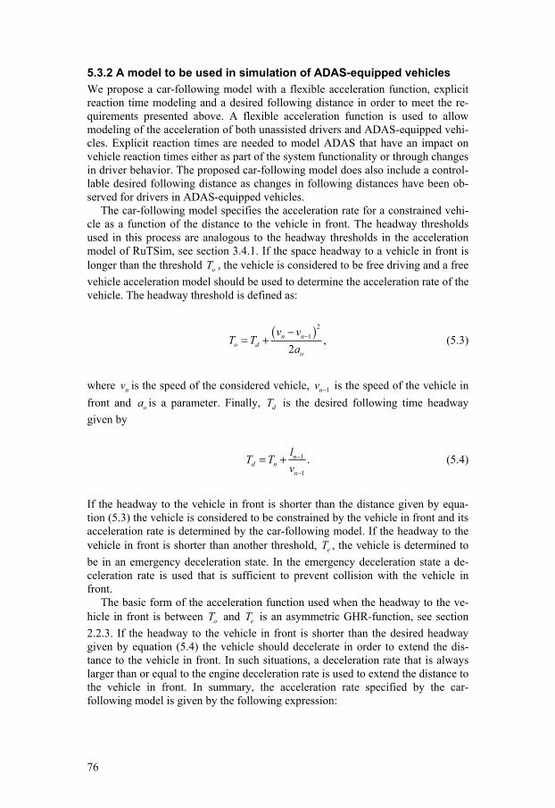
76

5.3.2 A model to be used in simulation of ADAS-equipped vehicles We propose a car-following model with a flexible acceleration function, explicit reaction time modeling and a desired following distance in order to meet the re-quirements presented above. A flexible acceleration function is used to allow modeling of the acceleration of both unassisted drivers and ADAS-equipped vehi-cles. Explicit reaction times are needed to model ADAS that have an impact on vehicle reaction times either as part of the system functionality or through changes in driver behavior. The proposed car-following model does also include a control-lable desired following distance as changes in following distances have been ob-served for drivers in ADAS-equipped vehicles.

The car-following model specifies the acceleration rate for a constrained vehi-cle as a function of the distance to the vehicle in front. The headway thresholds used in this process are analogous to the headway thresholds in the acceleration model of RuTSim, see section 3.4.1. If the space headway to a vehicle in front is longer than the threshold oT , the vehicle is considered to be free driving and a free vehicle acceleration model should be used to determine the acceleration rate of the vehicle. The headway threshold is defined as:

( )21 ,

2n n

o do

v vT T

a−−

= + (5.3)

where nv is the speed of the considered vehicle, 1nv − is the speed of the vehicle in front and oa is a parameter. Finally, dT is the desired following time headway given by

1

1

.nd n

n

lT Tv

−

−

= + (5.4)

If the headway to the vehicle in front is shorter than the distance given by equa-tion (5.3) the vehicle is considered to be constrained by the vehicle in front and its acceleration rate is determined by the car-following model. If the headway to the vehicle in front is shorter than another threshold, eT , the vehicle is determined to be in an emergency deceleration state. In the emergency deceleration state a de-celeration rate is used that is sufficient to prevent collision with the vehicle in front.

The basic form of the acceleration function used when the headway to the ve-hicle in front is between oT and eT is an asymmetric GHR-function, see section 2.2.3. If the headway to the vehicle in front is shorter than the desired headway given by equation (5.4) the vehicle should decelerate in order to extend the dis-tance to the vehicle in front. In such situations, a deceleration rate that is always larger than or equal to the engine deceleration rate is used to extend the distance to the vehicle in front. In summary, the acceleration rate specified by the car-following model is given by the following expression:

77

( )( )

( )( )

1

1 1

1

1 1

min , ,

( )

, ,

n n enginen n e d

n n nn n

n nn d o

n n n

v vv d T T T

x x la t

v vv T T T

x x l

βγ

βγ

ατ

α

−

− −

−

− −

− ≤ <

− − + = − ≤ ≤ − −

(5.5)

where T is the current headway to the vehicle in front, nx is the position of the considered vehicle, 1nx − is the position of the vehicle in front, 1nl − is the length of the vehicle in front, engine

nd is the engine deceleration rate and ,α β and γ are model parameters. Different parameter values are used for acceleration and decel-eration situations, i.e. acceleration parameters are used if ( )1sgn 0n nv v− − ≥ and deceleration parameters are used otherwise.

If the acceleration rate given by equation (5.5) is larger than the acceleration rate prescribed by the free vehicle acceleration model used in the simulation it is not desirable for the follower to adopt the car-following acceleration rate. In such cases the acceleration rate specified by the free vehicle acceleration model is ap-plied even though the headway to the vehicle in front is shorter than the threshold given by equation (5.3). Moreover, if the vehicle is moving faster than its desired speed it is not desirable to accelerate although equation (5.5) prescribes a positive acceleration rate. The free vehicle acceleration model is therefore used to deceler-ate vehicles in such situations.

In simulations including ADAS-equipped vehicles the parameters of equation (5.5) should be set to reflect the acceleration behavior of the modeled ADAS. Dis-tributions of desired following time gaps and reaction times for vehicles equipped with specific ADAS should also be utilized. It may also be appropriate to use dif-ferent driver/vehicle behavior for different traffic situations, e.g. based on vehicle speeds. These behavioral driver/vehicle data can be obtained from the system specifications of the ADAS to be simulated together with driving simulator or instrumented vehicle studies of drivers in ADAS-equipped vehicles.

5.4 Computational Results The car-following model described in the previous section has been included in RuTSim. The standard car-following model of RuTSim is replaced by the pro-posed car-following model for ADAS evaluation.

Simulation runs with varying driver reaction times and desired following dis-tances have then been performed using the extended RuTSim model to study the importance of changes in driver behavior when simulating traffic including ADAS-equipped vehicles for safety evaluation purposes. The aim of the simula-tion study is to investigate the potential to use traffic simulation for ADAS safety evaluation and to study necessary features of a traffic simulation model to be used for this task. The safety impacts of different reaction times and following dis-tances has been studied through the extended time-to-collision safety measures presented above in equations (5.1) and (5.2), i.e. TET and TIT . The TET and TIT measures where chosen due to their ability to indicate road safety on a stretch of road. Other measures based on, for example, maximum deceleration rate could also have been appropriate for this task. Values of the car-following model pa-

78

rameters ,α β and γ in equation (5.5) published by Yang (1997) were used in all simulations.

In order to permit simulation of traffic including vehicles with different behav-ior, the traffic generation process of RuTSim has been modified to allow individ-ual vehicle reaction times and desired following time gaps. For each vehicle type, i.e. cars and different types of trucks, the model allows specification of distinct categories with different reaction time and desired following time gap distribu-tions. Vehicles are then generated according to these specifications. In a future simulation of traffic including vehicles equipped with different types of ADAS, different vehicle categories can be used to represent the impact of the ADAS.

5.4.1 Implementation Driver reaction times are explicitly accounted for in the implementation. In a given time step the model computes and stores the acceleration rate given by the car-following model and the acceleration rate stored one reaction time earlier is assigned to the vehicle under consideration. This procedure is used for all situa-tions in which reaction times should be applied. When a following vehicle attains the speed of the vehicle in front and the distance to the leader is longer than the distance corresponding to the following vehicle’s desired following time gap, ac-celeration rate zero is assigned to the following vehicle. The next reaction of the following vehicle is analogously delayed one reaction time, i.e. the acceleration rates given by the car-following model is stored and acceleration rate zero is used until one reaction time has passed. The following vehicle is allowed to react im-mediately in emergency deceleration situations to avoid collisions between vehi-cles. In such situations, reaction time is not applied until the distance to the leader is longer than the desired following distance.

5.4.2 Simulation runs The 8 km long two-lane rural road studied in the previous chapter has been mod-eled in the extended RuTSim model. Traffic volumes of the average hour 2004 were used for all simulation runs. The traffic flow contained cars and three types of trucks with and without trailer. The truck percentage of the traffic was ap-proximately 15 %. The critical time-to-collision threshold used for calculation of the TET and TIT indicators has been set to 3 seconds in all simulations. This value was chosen based on literature, see e.g. (Minderhoud and Bovy, 2001; Archer, 2005), to distinguish safety critical situations from situations in which the driver remained in control.

Simulation runs with varying reaction times for cars was performed to isolate the impact of different reaction times on the safety indicators. Different reaction times can be thought of as corresponding to different types of ADAS. The reac-tion times of trucks were held constant at one second. This value was chosen to correspond to the reaction times of drivers without assistance of any ADAS. As a consequence, an indication of the impact of ADAS on surrounding unequipped vehicles is given by the relationship between the safety indicators for trucks and the reaction time of cars.

Figure 20 contains the resulting relationships between reaction time and the safety indicators. The TET indicator shown in the left-hand side of Figure 20 has been normalized by average journey time, jT , for the corresponding vehicle type.

79

The TET indicator shown in the graph is therefore the percentage of the journey time traveled with sub-critical time-to-collision to the vehicle in front. In similar fashion, the TIT indicator displayed in the right-hand side of Figure 20 has been normalized by the average journey time times the critical time to collision thresh-old, *

jT TTC⋅ . As a consequence, the TIT indicator shown in Figure 20 is a per-centage of the maximum attainable TIT . The error-bars shown in the graphs indicate 90 %-confidence intervals for the measures derived from the simulation. These confidence intervals have been constructed by assuming normally distrib-uted output from simulations with different random number seeds. The difference in confidence interval width between vehicle types is due to the smaller propor-tion of trucks in the traffic stream. As a consequence fewer trucks have been ob-served and the resulting confidence intervals become wider.

0 0.5 10

0.05

0.1

0.15

0.2

0.25

0.3

0.35

0.4

0.45

0.5

Reaction time (Cars) [s]

TET/

T j [%]

0 0.5 10

0.05

0.1

0.15

0.2

Reaction time (Cars) [s]

TIT/

(Tj ⋅

TTC* ) [

%]

CarsTrucks

Figure 20 TET for cars and trucks as a function of the reaction time of cars (left) and TIT for cars and trucks as a function of the reaction time of cars (right)

The left-hand side of Figure 20 indicates a linear relationship between TET and reaction time for cars. The time traveled with a sub-critical time-to-collision is proportional to the reaction time. Hence, shorter reaction times will increase safety and ADAS that shorten reaction times may therefore improve road safety. Trucks do not appear to be influenced by changes in the reaction time of cars ex-cept for small reaction times. This indicates that an ADAS that reduces driver reaction time will have restricted impact on surrounding unequipped vehicles. However, ADAS that result in very short reaction times may also have an impact on the safety of surrounding unequipped vehicles. One reason for this effect can be that if ADAS-equipped vehicles react very fast to situations ahead there is more time for unequipped vehicles traveling behind to react before the critical situation is reached.

80

The right-hand side of Figure 20 shows similar relationships between TIT and reaction time. Consequently, as TIT can be viewed as a measure of the severity of the critical situations, the longer reaction times the more severe critical situations. The severity of the critical situations for trucks is not influenced by changes in the reaction time of cars except for short reaction times. There is a tendency that the TIT indicator for trucks decreases with decreasing car reaction time for short reac-tion times. This indicates, as discussed above, that ADAS that result in short reac-tion times may improve safety not only for the equipped vehicles but also for surrounding unequipped vehicles. The relationship between TIT and reaction time together with the evident relationship between reaction time and TET shown in left-hand side of Figure 20 indicates the importance of explicit reaction time modeling in a traffic simulation model to be used for ADAS safety evaluation.

Simulation runs with varying desired following time gaps for cars has also been performed to study the impact of this behavioral parameter. As in the ex-periment with varying reaction times presented above, different desired following time gaps can also be thought of as corresponding to different ADAS. Default desired following time gap distributions was used for trucks to allow interpreta-tion of the safety indicator for trucks as an indicator of the impact on surrounding unequipped vehicles.

Figure 21 contains the resulting relationships between desired following time gap for cars and the safety indicators. The TET and TIT indicators shown in the right- and left-hand sides of Figure 21 respectively have been normalized in the same way as the indicators shown in Figure 20. The confidence intervals ex-pressed by the error-bars in Figure 21 have also been constructed in the same way as the confidence intervals shown in Figure 20.

81

1 1.5 2 2.5 30

0.05

0.1

0.15

0.2

0.25

0.3

0.35

0.4

0.45

0.5

Desired following time gap (Cars) [s]

TET/

T j [%]

1 1.5 2 2.5 30

0.05

0.1

0.15

0.2

Desired following time gap (Cars) [s]

TIT/

(Tj ⋅

TTC* ) [

%]

CarsTrucks

Figure 21 TET for cars and trucks as a function of the desired following time gap of cars (left) and TIT for cars and trucks as a function of the desired following time gap of cars (right)

The TET indicator increases exponentially with decreasing desired following dis-tance. This indicates the importance of desired following time gap as a determin-ing factor for the time traveled with sub-critical time-to-collision. As a consequence, ADAS that result in decreased following distances may also result in safety reductions if the decrease in following distance is not combined with, for example, a shortening of the reaction time. The TET indicator for trucks does not appear to be influenced by reduced desired following time gaps of cars except for short desired following time gaps. The graph indicates that the TET for trucks may increase as the desired following time gaps of cars decrease for short desired following time gaps. For this reason, ADAS that result very short following dis-tances may also reduce safety for surrounding unequipped vehicles. This effect may be due to the fact that if an ADAS-equipped vehicle travels closer to its leader then the vehicle behind the equipped vehicle is also likely to be closer to the vehicle in front of the equipped vehicle. The vehicle behind the ADAS-equipped vehicle will therefore also have shorter time to react to any critical situa-tion that may occur. As a consequence, care should be taken when designing ADAS that result in shortened following distances. It becomes very important to assess the effects on the traffic system as a whole in such situations.

The relationship between TIT and desired following time gap is shown in the right-hand side of Figure 21. The graph indicates that the severity of the critical situations increase exponentially with decreasing desired following time gaps. Trucks are not to any large extent influenced by decreased desired following time gaps of cars. As in the previously presented graphs there is an indication that trucks may be affected by short desired following time gaps of cars. As both

82

TET and TIT for cars increase exponentially with decreasing desired following time gaps, one may conclude that controllable desired following time gaps is an important feature of a traffic simulation model to be used for ADAS safety evaluation.

We have also studied average journey speed for cars as a function of reaction time and desired following time gap to compare the sensitivity of the TIT and TET indicators to the sensitivity of standard level-of-service measures derived from traffic simulation models. Figure 22 contains these relationships between journey speed and driver behavior expressed as reaction time and desired follow-ing time gap. The confidence intervals shown in Figure 22 have been constructed in the same way as the confidence intervals in the two previous figures.

0 0.5 124.5

24.6

24.7

24.8

24.9

25

25.1

25.2

25.3

25.4

25.5

Ave

rage

jour

ney

spee

d [m

/s]

Reaction time (Cars) [s]1 1.5 2 2.5 3

24.5

24.6

24.7

24.8

24.9

25

25.1

25.2

25.3

25.4

25.5

Desired following time gap (Cars) [s]

Figure 22 Average journey speed for cars as a function of the reaction time of cars (left) and the desired following time gap of cars (right)

As can be seen in the left-hand side of Figure 22, there is no clear relationship between reaction time and average journey speed. Therefore, it is not possible to draw conclusions on road safety due to changes in reaction time based on average journey speed. In addition, ADAS that only affect reaction times will not have any major consequences for the journey speed. The right-hand side of Figure 22 shows a tendency that increased desired following time gaps result in decreased journey speed. As a consequence, one may conclude that ADAS that have an im-pact on following distances will result in some changes in average journey speeds. However, the weak relationship indicates that average journey speed will be a blunt tool for safety assessments of ADAS that affect the desired following dis-tance.

In summary, the results of the simulation runs indicate clear relationships be-tween both reaction time and desired following time gap and the derived safety indicators. These findings indicate that traffic simulation will be of use in assess-

83

ments of the safety effects of ADAS that have an impact on driver behavior and the traffic flow properties.

5.5 Conclusions Necessary features of a traffic simulation model to be used for safety evaluations of ADAS have been described. ADAS have an impact on traffic through the ac-tual system functionalities and through changes in driver behavior due to the ADAS. A traffic simulation model to be used for simulation of traffic including ADAS-equipped vehicles should therefore include both of these aspects. Changes in reaction times, following distances and speeds have been observed for drivers in vehicles equipped with longitudinal control ADAS. The car-following model used for simulation of longitudinal control ADAS should consequently allow modeling of these behavioral changes.

A car-following model including a flexible acceleration function, explicit reac-tion time and a desired following distance has been proposed for use in simula-tions of traffic including ADAS-equipped vehicles. Simulation runs with the proposed car-following model have been performed to study the impact of differ-ent driver/vehicle behavior on safety related traffic measures derived from the simulation. The results show that driver/vehicle behavior has a substantial impact on the derived safety measures. Modeling of driver/vehicle behavior is therefore essential for reliable safety evaluations of ADAS.

The simulation runs presented in this work give inspiration for other tests. For example, it will be of interest to study different ADAS penetration levels by intro-ducing additional vehicle categories with different driver behavior. Another find-ing that demands further analysis is the observed changes in the safety indicators for other vehicle categories, i.e. trucks in figures above, for short reaction times and following time gaps of cars. This may indicate that ADAS that shorten reac-tion times sufficiently also provides safety benefits for surrounding unequipped vehicles. Analogously, ADAS that result in shorter desired following time gaps may also reduce safety for unequipped vehicles if not combined with a counterac-tive system that, for example, reduce driver reaction times. The effect of many ADAS is likely to increase with increasing traffic volumes as increasing traffic volumes also imply increasing interactions between vehicles. A study of the safety implications of ADAS under different traffic conditions would therefore be of interest. As reaction times and following distances are shown to have substantial impacts on the safety indicators it would also be interesting to study the impact of different values on the car-following model parameters. Modeling and simulation of specific ADAS is also subjects for future research. This work includes incorpo-ration of system functionalities and observed driver behavior in the simulation model. The work described in this paper has focused on longitudinal control ADAS and requirements imposed on the car-following model. On two-lane rural roads without separation of oncoming lanes, there is also a potential to improve safety with ADAS that support overtakings carried through in the oncoming lane. The extended RuTSim model will be used to simulate traffic including such over-taking aids to assess this potential.

85

6. Concluding Remarks and Future Research A traffic simulation framework for rural road environments has been developed. The developed model, RuTSim, draws upon the modeling logic originally devel-oped for VTISim (Brodin and Carlsson, 1986). VTISim is a proven model for simulation of uninterrupted traffic on two-lane rural roads. RuTSim extends the area of application for rural road traffic simulation and it handles both undivided two-lane highways and highways with separated oncoming lanes. Impacts of un-signalized intersections and roundabouts are also accounted for. The model has been implemented in a modular way to allow extension and/or modification of the model for future areas of application. Possible future areas of application besides level-of-service studies include assessments of the environmental impact of traffic and simulation based road safety evaluations.

The RuTSim framework has been applied in a study of four rural road design alternatives. This simulation study illustrates how the RuTSim model can be ap-plied in level-of-service studies. Within the simulation study, the model is cali-brated and validated for an existing two-lane highway in the southern part of Sweden. A good general agreement between the simulation results and the field data is established. Some difficulties are identified in connection with simulation scenarios including large traffic volumes. There is a need to improve the gap ac-ceptance logic and the lane drop merging algorithms used in heavy traffic condi-tions. The RuTSim model is also currently calibrated and validated for additional Swedish rural highways with as well as without separated oncoming lanes.

The use of traffic simulation for studies of the road safety impact of Advanced Driver Assistance Systems (ADAS) is investigated in the last part of this work. Necessary features of a simulation model to be used for ADAS evaluation are identified and a car-following model suitable for simulation of traffic including vehicles equipped with longitudinal control ADAS is proposed. The proposed car-following model has been implemented in the RuTSim framework to study the importance of some important model properties. The result of this study is that it is important to consider the ADAS system functionality as well as the driver be-havior in ADAS-equipped vehicles. Safety related traffic measures should also be derived from the simulation output. The extended RuTSim model will be a useful tool for future studies of the effects of ADAS in rural environments.

Subjects for future research include developments of improved models for simulation of large traffic volumes. This includes improvement of the gap-acceptance logic for vehicles entering the road at intersections and enhancement of the lane drop merging algorithm. There is also a possibility to improve the model by introducing stochastic elements in the car-following model to account for imperfect reactions of the following vehicle.

One of the most interesting subjects for future research is however further work on traffic simulation for road safety evaluations in general and evaluations of the effects of ITS and ADAS in particular. The next steps on the path outlined by this work are studies of the effect of different ADAS penetration levels and the impact of ADAS under different traffic conditions. The overall safety effect of ADAS is likely largely dependent on the penetration level. It is for this reason interesting to investigate the relationship between road safety and the ADAS penetration in the traffic system. The work in this thesis has also indicated that vehicles may be in-fluenced by surrounding ADAS-equipped vehicles. This effect may be important for the overall benefit of an ADAS and should consequently be investigated prior

86

to the introduction of the ADAS in the traffic system. The effect of ADAS is also likely to increase with increasing traffic volumes since this, in general, will imply an increased number of critical situations. A study of the effect of ADAS under different traffic conditions is therefore important to assess the ADAS road safety effect. Modeling and simulation of specific longitudinal control ADAS are also subjects for future research. This includes modeling of ADAS system functional-ities and driver behavior in ADAS-equipped vehicles. The driver behavior in ADAS-equipped vehicles may be obtained from driving simulator or instrumented vehicle studies.

Another area for future research is simulation of lateral control ADAS. The safety on narrow two-lane rural highways is discussed in an ongoing debate. It is not possible to separate the oncoming lanes on a narrow carriageway. Other safety improving countermeasures must therefore be investigated. Examples of such countermeasures are lateral control ADAS, e.g. overtaking aids, and rumble strips installed in the center line of the carriageway. The RuTSim framework will in the near future be used to study the traffic effects on rural roads with center line rum-ble strips and other overtaking aids.

87

References Allen, R. W., D. Harwood, J. P. Christos and W. D. Glauz (2000). The Capability

and Enhancement of VDANL and TWOPAS for Analyzing Vehicle Per-formance on Upgrades and Downgrades Within IHSDM. Federal Highway Administration, McLean, VA.

Archer, J. (2005). Indicators for Traffic Safety Assessment and Prediction and Their Application in Micro-Simulation Modelling: A Study of Urban and Suburban Intersections. Department of Infrastructure, Royal Institute of Technology, Stockholm.

Barceló, J. and J. Casas (2002). Dynamic Network Simulation with Aimsun. Inter-national Symposium on Transport Simulation, Yokohama

Barceló, J., A.-G. Dumont, L. Montero, J. Perarnau and A. Torday (2003). Safety Indicators for Microsimulation-Based Assessments. Transportation Re-search Board Annual Meeting 2003, Washington D.C.

Bolling, A. and O. Junghard (1988). Dokumentation av program i VTIs trafik-simuleringsmodell (Documentation of Programs in the VTI Traffic Simula-tion Model, in Swedish). Swedish National Road and Transport Research Institute, Linköping.

Botha, J. L., X. Zeng and E. C. Sullivan (1993). Comparison of the Performance of TWOPAS and TRARR Models When Simulating Traffic on Two-Lane Highways with Low Design Speeds. Transportation Research Record 1398: 7-16.

Brackstone, M. and M. McDonald (1999). Car-Following: A Historical Review. Transportation Research Part F 2: 181-196.

Branston, D. (1976). Model of Single Lane Time Headway Distributions. Trans-portation Science 10(2): 125-148.

Brodin, A. and A. Carlsson (1986). The VTI Traffic Simulation Model. Swedish National Road and Transport Research Institute, Linköping.

Burghout, W. (2004). Hybrid Microscopic-Mesoscopic Traffic Simulation. De-partment of Infrastructure, Royal Institute of Technology, Stockholm.

Cambridge Systematics (2004). NGSIM Task E.1-1: Core Algorithms Assessment (Final Report). Oakland.

Carlsson, A. (1990). Trafikantbeteende på 13 m-väg. Studie av passeringar och omkörningar (Road-User Behaviour on 13 m-Roads. A study of Overtak-ings and Passages, in Swedish). Swedish National Road and Transport Re-search Institute, Linköping.

Carlsson, A. (1991). Trafikantbeteende på 8-9 m-väg. Studie av omkörningar (Road-User Behaviour on 8-9 m-Roads. A Study of Overtakings, in Swed-ish). Swedish National Road and Transport Research Institute, Linköping.

Carlsson, A. (1993a). Beskrivning av VTIs trafiksimuleringsmodell (Description of the VTI Traffic Simulation Model, in Swedish). Swedish National Road and Transport Research Institute, Linköping.

Carlsson, A. (1993b). Linjeföring och omkörningssikt (Road Alignment and Over-taking Sight, in Swedish). Swedish National and Transport Research Insti-tute, Linköping.

Carlsson, A. and U. Björketun (2005). Trafikvariation över året (Traffic Variation During the Year, in Swedish). Swedish National Road and Transport Re-search Institute, Linköping.

Carlsson, A. and U. Brüde (2003). Uppföljning av mötesfria vägar. Halvårsrap-port 2002:1 (Evaluation of Roads without Oncoming Traffic. Half-Yearly

88

Statement 2002:1, in Swedish). Swedish National Road and Transport Re-search Institute, Linköping.

Carlsson, A. and U. Brüde (2005). Uppföljning av mötesfria vägar. Halvårsrap-port 2004:2 (Evaluation of Roads without Oncoming Traffic. Half-Yearly Statement 2004:2, in Swedish). Swedish National Road and Transport Re-search Institute, Linköping.

Carlsson, A. and A. Tapani (2005a). Framkomlighet och fördröjningar på E22 Fjälkinge-Gualöv (Accessibility and Delays on the E22 Fjälkinge-Gualöv, in Swedish). Swedish National Road and Transport Research Institute, Linköping.

Carlsson, A. and A. Tapani (2005b). Rural Highway Design Analysis through Traffic Micro-simulation. Submitted for presentation at the 5th Interna-tional Symposium on Highway Capacity and Quality of Service, Yoko-hama

Daganzo, C. (1994). The Cell Transmission Model: A Dynamic Representation of Highway Traffic Consistent with the Hydrodynamic Theory. Transporta-tion Research B 28(4).

Daganzo, C. (1995). The Cell Transmission Model Part II: Network Traffic. Transportation Research B 29(2): 79-93.

Ehmanns, D. and H. Spannheimer (2004). ADASE II Roadmap (ADASE Deliver-able D2D Roadmap Development). Information Society Technologies, Brussels.

Flodas, N., A. Admitis, A. Keinath, K. Bengler and A. Engeln (2005). Review and Taxonomy of IVIS/ADAS Applications (AIDE Deliverable D2.1.2). Infor-mation Society Technologies, Brussels.

Fritzsche, H.-T. (1994). A Model for Traffic Simulation. Traffic Engineering and Control 5: 317 - 321.

Gazis, D. C., R. Herman and R. B. Potts (1959). Car-Following Theory of Steady-State Traffic Flow. Operations Research 7: 499-505.

Gazis, D. C., R. Herman and R. W. Rothery (1961). Nonlinear Follow-the-leader Models of Traffic Flow. Operations Research 9: 545-567.

Gettman, D. and L. Head (2003). Surrogate Safety Measures from Traffic Simula-tion Models. Transportation Research Record 1840: 104-115.

Gilliam, C. D. (1978). A Model for the Generation of various Traffic Characteris-tics. UK Department of Transport,

Gipps, P. G. (1981). A Behavioural Car-Following Model for Computer Simula-tion. Transportation Research B 15: 105-111.

Gipps, P. G. (1986). A Model for the Structure of Lane-changing Decisions. Transportation Research Part B 20(5): 403-414.

Harwood, D. W., A. D. May, I. B. Anderson, L. Lieman and A. R. Archilla (1999). Capacity and Quality of Service of Two-Lane Highways. Midwest Research Institute and University of California-Berkeley,

Hoban, C. J., R. J. Shepherd, G. J. Fawcett and G. K. Robinson (1991). A Model for Simulating Traffic on Two-Lane Rural Roads: User guide and manual for TRARR version 3.2. Australian Road Research Board, Victoria.

Hoogendoorn, S., P. and P. H. L. Bovy (2001). State-of-the-art of Vehicular Traf-fic Flow Modelling. Journal of Systems and Control Engineering 215(4): 283-303.

Hoogendoorn, S. P. (2005). ADAS Safety Impact on Rural and Urban Highways. Transportation Research Board Annual Meeting 2005, Washington D.C.

89

ITS Leeds (2000). SMARTEST. Institute for Transportation Studies, University of Leeds, Leeds.

Koorey, G. (2002). Assesment of Rural Road Simulation Modelling Tools. IPENZ Transportation Group Technical Conference, New Zealand

Leiman, L., A. R. Archilla and A. D. May (1998). Twopas Model Improvements. University of California, Berkeley California,

Leutzbach, W. (1988). Introduction to the Theory of Traffic Flow. Springer Ver-lag, Berlin.

Liu, R. and J. Tate (2004). Network Effects of Intelligent Speed Adaptation Sys-tems. Transportation 31: 297-325.

Lundgren, J. and A. Tapani (2005). Evaluation of Safety Effects of Driver Assis-tance Systems through Traffic Simulation. Submitted for presentation and publication to the Transportation Research Board, Washington D.C.

May, A. D. (1990). Traffic Flow Fundamentals. Prentice Hall, Upper Saddle River.

McLean, J. R. (1989). Two-Lane Highway Traffic Operations. Gordon and Breach Science Publishers, Amsterdam.

Messmer, A. and M. Papageorgiou (1990). Metanet: A Macroscopic Simulation Program for Motorway Networks. Traffic Engineering and Control 31: 466-470.

Miller, A. J. (1961). A Queuing Model Road Traffic Flow. Journal of the Royal Statistical Society 23(1): 64-75.

Miller, A. J. (1967). Queueing in Rural Traffic. Vehicular Traffic Science: 122-137. Elsevier, New York.

Minderhoud, M. M. and P. H. L. Bovy (2001). Extended Time-to-Collision Meas-ures for Road Traffic Safety Assessment. Accident Analysis and Preven-tion 33: 89-97.

PTV, VISSIM. http://www.english.ptv.de/cgi-bin/traffic/traf_vissim.pl, accessed Mar. 7, 2004.

Quadstone, Quadstone Paramics. http://www.paramics-online.com, accessed Mar. 8, 2004.

Saad, F., M. Hjälmdahl, J. Cañas, M. Alonso, P. Garayo, L. Macchi, F. Nathan, L. Ojeda, V. Papakostopoulos, M. Panou and E. Bekiaris (2004). Literature Review of Behavioural Effects (AIDE Deliverable D1.2.1). Information Society Technologies, Brussels.

SIKA (2000). Prognos för godstransporter 2010 (Freight Traffic Forecast 2010, in Swedish). Swedish Institute for Transport and Communications Analy-sis, Stockholm.

SIKA (2002). Persontransporternas utveckling till 2010 (The Development of Passenger Traffic Until 2010, in Swedish). Swedish Institute for Transport and Communications Analysis, Stockholm.

SRA (1995). CAPCAL 2 Model Description of Intersections without Signal Con-trol. Swedish Road Administration, Borlänge.

SRA (2001). Effektsamband 2000 (Effect Relationships 2000, in Swedish). Swed-ish Road Administration, Borlänge.

SRA (2004). Vägars och gators utformning (Road and Street Design, in Swedish). Swedish Road Administration, Borlänge.

Strömgren, P. (2002). Mikrosimulering av trafik i vägkorsning (Micro-Simulation of Intersection Traffic, in Swedish). Department of Infrastructure, Royal Institute of Technology, Stockholm.

90

Tanner, J. C. (1961). Delays on a Two-lane Road. Journal of the Royal Statistical Society 23(1): 38-63.

Tapani, A. (2005a). Traffic Simulation for Road Safety Assessment of Intelligent Transportation Systems. Modeling and Simulation for Public Safety (Sim-Safe 2005), Linköping, The Programming Environments Laboratory, De-partment of Computer and Information Science, Linköping University.

Tapani, A. (2005b). A Versatile Model for Rural Road Traffic Simulation. Ac-cepted for publication in Transportation Research Record.

Taylor, N. B. (2003). The CONTRAM Dynamic Traffic Assignment Model. Net-works and Spatial Economics 3: 297-322.

TSS, AIMSUN. http://www.aimsun.com, accessed Mar. 8, 2004. Wiedemann, R. and U. Reiter (1992). Microscopic Traffic Simulation: The Simu-

lation System MISSION, Background and Actual State (Project ICARUS (V1052) Final Report). CEC, Brussels.

Yang, Q. (1997). A Simulation Laboratory for Evaluation of Dynamic Traffic Management Systems. Massachusetts Institute of Technology, Cambridge.

Appendix A Page 1(2)

A. Overtaking Parameters

A k Overtaken vehicle Road width

Sight limitation

Type of overtaking

3.30 0.00350 Car < 70 km/h < 11 m Natural Accelerating11.8 0.01220 Car < 70 km/h < 11 m Natural Flying 11.0 0.00460 Car < 70 km/h < 11 m Oncoming Accelerating11.5 0.00988 Car < 70 km/h < 11 m Oncoming Flying 6.30 0.00910 Car < 70 km/h ≥ 11 m Natural Accelerating2.30 0.01430 Car < 70 km/h ≥ 11 m Natural Flying 7.50 0.00700 Car < 70 km/h ≥ 11 m Oncoming Accelerating2.30 0.01403 Car < 70 km/h ≥ 11 m Oncoming Flying 3.78 0.00334 Car < 90 km/h < 11 m Natural Accelerating11.8 0.01220 Car < 90 km/h < 11 m Natural Flying 11.0 0.00430 Car < 90 km/h < 11 m Oncoming Accelerating11.5 0.00988 Car < 90 km/h < 11 m Oncoming Flying 6.90 0.00867 Car < 90 km/h ≥ 11 m Natural Accelerating3.00 0.01207 Car < 90 km/h ≥ 11 m Natural Flying 7.50 0.00664 Car < 90 km/h ≥ 11 m Oncoming Accelerating3.00 0.01207 Car < 90 km/h ≥ 11 m Oncoming Flying 4.30 0.00317 Car ≥ 90 km/h < 11 m Natural Accelerating11.8 0.01220 Car ≥ 90 km/h < 11 m Natural Flying 11.0 0.00399 Car ≥ 90 km/h < 11 m Oncoming Accelerating11.5 0.00988 Car ≥ 90 km/h < 11 m Oncoming Flying 7.50 0.00822 Car ≥ 90 km/h ≥ 11 m Natural Accelerating6.00 0.00988 Car ≥ 90 km/h ≥ 11 m Natural Flying 7.50 0.00664 Car ≥ 90 km/h ≥ 11 m Oncoming Accelerating6.00 0.00988 Car ≥ 90 km/h ≥ 11 m Oncoming Flying

6.10 0.00440 Truck or Buss < 70 km/h < 11 m Natural Accelerating

37.0 0.01480 Truck or Buss < 70 km/h < 11 m Natural Flying

11.65 0.00430 Truck or Buss < 70 km/h < 11 m Oncoming Accelerating

13.74 0.00920 Truck or Buss < 70 km/h < 11 m Oncoming Flying

3.30 0.00510 Truck or Buss < 70 km/h ≥ 11 m Natural Accelerating

1.40 0.01270 Truck or Buss < 70 km/h ≥ 11 m Natural Flying

4.20 0.00370 Truck or Buss < 70 km/h ≥ 11 m Oncoming Accelerating

1.40 0.01270 Truck or Buss < 70 km/h ≥ 11 m Oncoming Flying

6.90 0.00420 Truck or Buss < 90 km/h < 11 m Natural Accelerating

37.0 0.01480 Truck or Buss < 90 km/h < 11 m Natural Flying

Appendix A Page 2(2)

11.65 0.00403 Truck or Buss < 90 km/h < 11 m Oncoming Accelerating

13.74 0.00920 Truck or Buss < 90 km/h < 11 m Oncoming Flying

3.60 0.00484 Truck or Buss < 90 km/h ≥ 11 m Natural Accelerating

1.61 0.01074 Truck or Buss < 90 km/h ≥ 11 m Natural Flying

4.20 0.00347 Truck or Buss < 90 km/h ≥ 11 m Oncoming Accelerating

1.61 0.01074 Truck or Buss < 90 km/h ≥ 11 m Oncoming Flying

6.90 0.00420 Truck or Buss ≥ 90 km/h < 11 m Natural Accelerating

37.0 0.01480 Truck or Buss ≥ 90 km/h < 11 m Natural Flying

11.65 0.00403 Truck or Buss ≥ 90 km/h < 11 m Oncoming Accelerating

13.74 0.00920 Truck or Buss ≥ 90 km/h < 11 m Oncoming Flying

3.60 0.00484 Truck or Buss ≥ 90 km/h ≥ 11 m Natural Accelerating

1.61 0.01074 Truck or Buss ≥ 90 km/h ≥ 11 m Natural Flying

4.20 0.00347 Truck or Buss ≥ 90 km/h ≥ 11 m Oncoming Accelerating

1.61 0.01074 Truck or Buss ≥ 90 km/h ≥ 11 m Oncoming Flying

6.90 0.00331 Truck with trailer - < 11 m Natural Accelerating

37.0 0.01480 Truck with trailer - < 11 m Natural Flying

14.0 0.00353 Truck with trailer - < 11 m Oncoming Accelerating

13.74 0.00920 Truck with trailer - < 11 m Oncoming Flying

4.20 0.00484 Truck with trailer - ≥ 11 m Natural Accelerating

2.08 0.00532 Truck with trailer - ≥ 11 m Natural Flying

4.20 0.00347 Truck with trailer - ≥ 11 m Oncoming Accelerating

2.08 0.00532 Truck with trailer - ≥ 11 m Oncoming Flying

Source: Carlsson (1993a)

Appendix B Page 1(1)

B. Critical Time Gaps Main road speed limit 50 km/h 70 km/h 90 km/h

Intersection control Yield Stop Yield Stop Yield Stop

Main road left 4.8 s 4.8 s 5.7 s 5.7 s 6.7 s 6.7 s

Minor road right 5.0 s 5.7 s 5.9 s 6.6 s 6.9 s 7.5 s Turn

Movement Minor road left 5.3 s 6.0 s 6.2 s 6.9 s 7.2 s 7.8 s

Source: SRA (1995)

Appendix C Page 1(2)

C. Default Parameter Values Scalars Parameter Value Dimension Page

0v 30.83 [ ]/m s 26

carλ 0 - 27

truckλ 0.3 - 27

(3 4 )truck with trailer axlesλ − 0.5 - 27

( 5 )truck with trailer axlesλ ≥ 0.5 - 27 81

mv 27.75 [ ]/m s 27 a 0.042 [ ]s 27 b 0.15 2 /s m 28 d 0.050 - 29

1q 0.6 - 30

2q -0.8 - 30

3q -0.2 - 30

normala 0.5 2/m s 32 A

CarC 30.331 10−⋅ 1m− 35 A

TruckC 30.170 10−⋅ 1m− 35

(3 4 )A

Truck with trailer axlesC − 30.140 10−⋅ 1m− 35

( 5 )A

Truck with trailer axlesC ≥ 30.105 10−⋅ 1m− 35 1R

CarC 0.106 2/m s 35 1R

TruckC 0.056 2/m s 35 1

(3 4 )RTruck with trailer axlesC − 0.052 2/m s 35

1( 5 )

RTruck with trailer axlesC ≥ 0.051 2/m s 35

2RCarC 0.0 1s− 35

2RTruckC 0.0 1s− 35

2(3 4 )

RTruck with trailer axlesC − 0.0 1s− 35

2( 5 )

RTruck with trailer axlesC ≥ 0.0 1s− 35

mind 5.0 [ ]s 37

oa 3.0 2/m s 41

CFS 1.5 - 41

minT 0.5 [ ]s 43 engined 0.5 2/m s 43

Appendix C Page 2(2)

maxd 7.0 2/m s 43 ξ 50 [ ]m 43

maxovtkl 1000 [ ]m 45

minovtkv∆ 0.5 [ ]/m s 45

restovtkl 200 [ ]m 46

minflyings 100 [ ]m 46

minaccs 200 [ ]m 46

η 0.6 - 46 desovtkv 6.0 [ ]/m s 47 redpassedv 0.9 - 47 turnnormala 1.5 2/m s 50

intersecmint 2.0 [ ]s 50 truckgapt 0.5 [ ]s 51 follow

gapt 0.6 - 53 Distributions Parameter Mean Standard

deviationMin Max Dimension Page

0Carv 30.83 3.19 22.85 38.81 [ ]/m s 26

0Truckv 26.53 2.92 19.23 33.83 [ ]/m s 26

0 (3 4 )Truck with trailer axlesv − 24.31 1.50 20.81 28.81 [ ]/m s 26

0 ( 5 )Truck with trailer axlesv ≥ 24.31 1.50 20.81 28.81 [ ]/m s 26

Carp 19.0 7.0 5.0 41.0 2 3/m s 35

Truckp 11.5 2.5 3.0 25.0 2 3/m s 35

(3 4 )Truck with trailer axlesp − 6.5 1.5 2.0 14.0 2 3/m s 35

( 5 )Truck with trailer axlesp ≥ 5.5 1.0 2.0 12.0 2 3/m s 35

CarT 2.0 1.0 - - [ ]s 35

TruckT 2.25 1.1 - - [ ]s 35

(3 4 )Truck with trailer axlesT − 2.5 1.2 - - [ ]s 35

( 5 )Truck with trailer axlesT ≥ 2.5 1.2 - - [ ]s 35