A Time Series Weather Radar Simulator Based on High

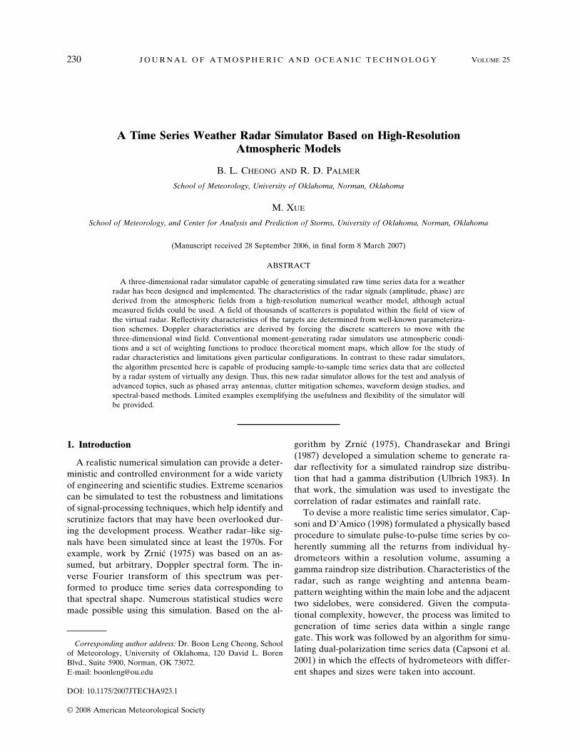
A Time Series Weather Radar Simulator Based on High-ResolutionAtmospheric Models

B. L. CHEONG AND R. D. PALMER

School of Meteorology, University of Oklahoma, Norman, Oklahoma

M. XUE

School of Meteorology, and Center for Analysis and Prediction of Storms, University of Oklahoma, Norman, Oklahoma

(Manuscript received 28 September 2006, in final form 8 March 2007)

ABSTRACT

A three-dimensional radar simulator capable of generating simulated raw time series data for a weatherradar has been designed and implemented. The characteristics of the radar signals (amplitude, phase) arederived from the atmospheric fields from a high-resolution numerical weather model, although actualmeasured fields could be used. A field of thousands of scatterers is populated within the field of view ofthe virtual radar. Reflectivity characteristics of the targets are determined from well-known parameteriza-tion schemes. Doppler characteristics are derived by forcing the discrete scatterers to move with thethree-dimensional wind field. Conventional moment-generating radar simulators use atmospheric condi-tions and a set of weighting functions to produce theoretical moment maps, which allow for the study ofradar characteristics and limitations given particular configurations. In contrast to these radar simulators,the algorithm presented here is capable of producing sample-to-sample time series data that are collectedby a radar system of virtually any design. Thus, this new radar simulator allows for the test and analysis ofadvanced topics, such as phased array antennas, clutter mitigation schemes, waveform design studies, andspectral-based methods. Limited examples exemplifying the usefulness and flexibility of the simulator willbe provided.

1. Introduction

A realistic numerical simulation can provide a deter-ministic and controlled environment for a wide varietyof engineering and scientific studies. Extreme scenarioscan be simulated to test the robustness and limitationsof signal-processing techniques, which help identify andscrutinize factors that may have been overlooked dur-ing the development process. Weather radar–like sig-nals have been simulated since at least the 1970s. Forexample, work by Zrnic (1975) was based on an as-sumed, but arbitrary, Doppler spectral form. The in-verse Fourier transform of this spectrum was per-formed to produce time series data corresponding tothat spectral shape. Numerous statistical studies weremade possible using this simulation. Based on the al-

gorithm by Zrnic (1975), Chandrasekar and Bringi(1987) developed a simulation scheme to generate ra-dar reflectivity for a simulated raindrop size distribu-tion that had a gamma distribution (Ulbrich 1983). Inthat work, the simulation was used to investigate thecorrelation of radar estimates and rainfall rate.

To devise a more realistic time series simulator, Cap-soni and D’Amico (1998) formulated a physically basedprocedure to simulate pulse-to-pulse time series by co-herently summing all the returns from individual hy-drometeors within a resolution volume, assuming agamma raindrop size distribution. Characteristics of theradar, such as range weighting and antenna beam-pattern weighting within the main lobe and the adjacenttwo sidelobes, were considered. Given the computa-tional complexity, however, the process was limited togeneration of time series data within a single rangegate. This work was followed by an algorithm for simu-lating dual-polarization time series data (Capsoni et al.2001) in which the effects of hydrometeors with differ-ent shapes and sizes were taken into account.

Corresponding author address: Dr. Boon Leng Cheong, Schoolof Meteorology, University of Oklahoma, 120 David L. BorenBlvd., Suite 5900, Norman, OK 73072.E-mail: [email protected]

230 J O U R N A L O F A T M O S P H E R I C A N D O C E A N I C T E C H N O L O G Y VOLUME 25

DOI: 10.1175/2007JTECHA923.1

© 2008 American Meteorological Society

JTECH2128

For numerous applications, it is often not necessaryto generate time series data when realistic momentmaps would suffice. For example, Krajewski et al.(1993) used a simulation scheme to generate radar-estimated rainfall fields without simulating time seriesdata. Radar measurements, that is, reflectivity and dif-ferential reflectivity, were directly derived from a two-dimensional stochastic space–time model of rainfallevents and drop size distribution. These radar-derivedmeasurements were then used to estimate rainfall rate.Anagnostou and Krajewski (1997) presented a similarsimulation procedure, with the addition of verticalstructure making a true three-dimensional model. Theantenna beam pattern within the 3-dB beamwidth ofthe main lobe was considered in the process of gener-ating the radar-estimated field.

Recently, May et al. (2007) developed a radar mo-ment simulator using output from a physically modeledthree-dimensional volume that is characterized by mul-tiple atmospheric fields. The simulated atmosphericvolume was generated from the high-resolution nu-merical weather simulations using the Advanced Re-gional Prediction System (ARPS; Xue et al. 2000,2001), in which the microphysical species including therainwater content is parameterized with a Marshall–Palmer drop size distribution (Marshall and Palmer1948). Similar to Capsoni et al. (2001), range and an-tenna weighting were considered. However, May et al.(2007) simulated a full three-dimensional volume, al-though just for spectral moments. Atmospheric effectssuch as anomalous propagation and attenuationthrough rain were investigated in detail. This simulatorprovides a powerful tool for the design and optimiza-tion of radar experiments under realistic atmosphericscenarios. Another recent example of a radar simulatorbased on atmospheric model output is the work of Cau-mont et al. (2006). This simulator was designed to be anintegral part of the high-resolution Meso-NH modeland has been used for sensitivity studies with the goal ofthe optimization of reflectivity assimilation. As such,the simulator was not designed with either Doppler orpolarimetric capabilities.

In the present work, the development of a radarsimulator, capable of generating realistic, three-dimensional, time series data, is presented. The simu-lator uses a Lagrangian framework with thousands ofscatterers moving with the wind field produced from ahigh-resolution atmospheric numerical model. The mo-tion of the targets causes variations in radar phase pro-ducing a Doppler shift. The radar signals are generatedby appropriately weighted integration of all targetswithin the resolution volume of the radar. A full three-dimensional view is possible by scanning this volume to

any desired location. This Lagrangian approach was in-spired by the work of Holdsworth and Reid (1995) inwhich radar time series for a very high frequency(VHF) wind profiler was generated using hundreds ofdiscrete point scatterers. Recent work by Cheong et al.(2004a) illustrated a more efficient and flexible ap-proach to incorporate realistic atmospheric parametersinto the simulator. In that work, a table lookup andfour-dimensional linear interpolation approach wereused to extract and infuse a set of pregenerated atmo-spheric parameters into the process of generating timeseries data. A similar approach is adopted here but forthe case of side-looking weather radars instead of aprofiler.

The next section provides the overall structure of theradar simulator in addition to an overview of the nu-merical weather prediction model used. Useful com-ments on the use of interpolation and the proposedtable lookup procedures are outlined in section 3. Ex-amples using the simulator for two distinct radar con-figurations are provided in section 4. Finally, conclu-sions drawn from this research are given in the lastsection.

2. Algorithmic structure of the radar simulator

The proposed simulator produces time series samplesof a radar by coherently adding thousands of discretesignals from a simulation domain. Each discrete signalrepresents a reflection from a point scatterer, which isan amplitude-attenuated and phase-shifted replica ofthe transmitted pulse. In this simulator, the primarygoal is to derive realistic radar returns given an arbi-trary but known reflectivity field from the atmosphericmodel ARPS. The reflectivity factor of each point scat-terer is set to be a function of its position within thesimulation domain while the phase is a function of itstwo-way path distance relative to the radar.

a. Overview of simulated atmospheric fields

The model-simulated dataset used to test our radarsimulator was produced by the ARPS model (Xue et al.2000, 2001), which was also used by May et al. (2007).The simulation used here has twice as much horizontalresolution, however. The ARPS is a fully compressibleand nonhydrostatic prediction model and its prognosticstate variables include wind components u, �, w, poten-tial temperature �, pressure p, the mixing ratios forwater vapor q�, cloud water qc, rainwater qr, cloud iceqi, snow qs, and hail qh, plus the turbulent kinetic en-ergy used by the 1.5-order subgrid-scale turbulent clo-sure scheme (see Xue et al. 2000, 2001, 2003 for details).

FEBRUARY 2008 C H E O N G E T A L . 231

For the current simulation, only the Kessler-type warm-rain microphysics is used. The simulation had a hori-zontal grid spacing of 25 m over a 48 km � 48 kmdomain during the period of time that data are usedhere, and the vertical grid is stretched and has a verticalspacing of 20 m at the surface. The simulation was fora tornadic supercell thunderstorm, and the storm wasinitiated by a thermal bubble in a horizontally homo-geneous environment defined by the 20 May 1977 DelCity, Oklahoma, sounding reported in Ray et al. (1981).

For the ARPS simulation, a horizontal resolution of50 m was first used and the entire simulation length wasover 4 h. An intense tornado developed after 3.5 h intothe simulation on the 50-m grid. Over a half-hour pe-riod centering on the time of the most intense tornado,a simulation using a 25-m resolution is performed, start-ing from an initial condition interpolated from the 50-mgrid. On this grid, an F4–F5 intensity tornado with amaximum ground-relative wind speed of over 120 m s�1

was obtained, with a pressure drop of over 80 hPa at thecenter of the tornado vortex. The simulated tornadovortex is about 200 m in diameter near the ground.Because of the small size and great intensity of thetornado vortex, spatial and temporal variabilities asso-ciated with the tornado are extreme. Gridded outputswith all model fields are available at 1-s intervals fromthis simulation. Detailed analysis of the simulated tor-nado is not very important here and will be reportedelsewhere.

In Xue et al. (2007), a single time output from thesame 25-m simulation near the time of most intensetornado was sampled by a simple Gaussian beam-pattern-based radar simulator to create simulated ra-dial velocity data for testing a variational velocityanalysis scheme combined with azimuthal oversam-pling. Liu et al. (2007) further used the dataset to test awavelet-based tornado detection algorithm.

In the proposed time series simulator, at any giveninstance in time, we will use two time level outputs fromthis 25-m model simulation as input to our radar emu-lator to create simulated observations.

b. Spatial/temporal evolution of scatterers

The radar echo from a transmitted pulse is a complexfunction of continuous fields of reflectivity and velocity,which depend on the true atmospheric conditions andare thus impractical for analytical solution. However, itis possible to approximate this function by using a largenumber of discrete scatterers that are randomly distrib-uted over the domain of interest. This is essentially aspatial sampling problem and the composite signal isobtained by coherently integrating the reflected signalsfrom each discrete scatterer. Compared to the volume-

scattering case, the returned signal from a single dis-crete scatterer is much simpler and analytical solutionsexist. Volume scattering is approximated by summingthe returned echoes from tens of thousands of discretescatterers that exist within the field of view of the radar.This process is termed Monte Carlo integration (Me-tropolis and Ulam 1949).

The coherently integrated signal from of all the dis-crete scatterers is referred to as the composite signal.Each sample of the composite signal is a complex sumof the baseband signal from all the individual scatterers,which can be expressed mathematically as follows:

x � �k�0

N�1

A�k� exp�j��k� � N , �1�

where superscript (·)(k) indicates the index of the dis-crete scatterers, N is the total number of scatterers, A(k)

represents the amplitude of the signal from the kth scat-terer, �(k) represents the phase of the kth scatterer, andN represents additive white Gaussian noise signal.Equation (1) is the general form for producing the com-posite signal and can be readily extended to simulatesystems that use multiple receivers, multiple frequen-cies, and/or multiple pulse repetition times (PRTs), forexample.

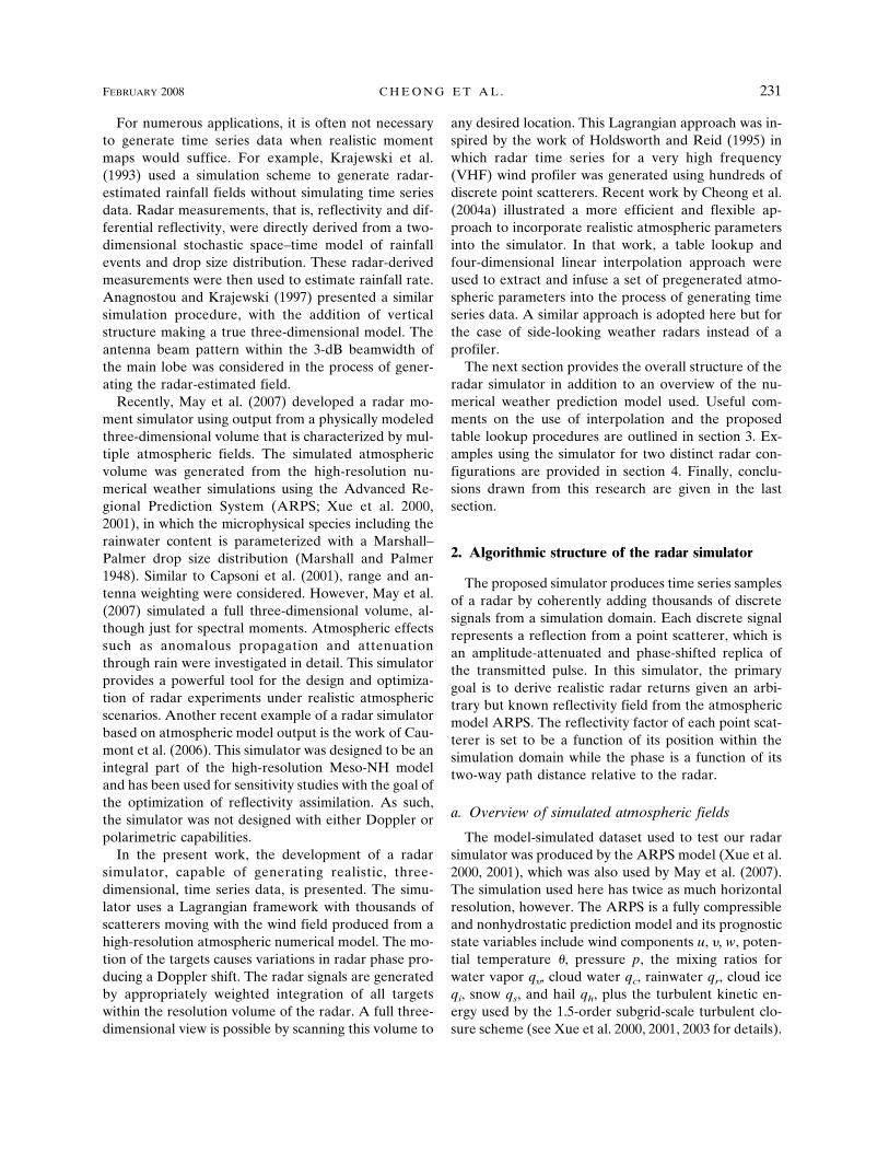
Figure 1 is an artist’s depiction of the general struc-ture of the proposed weather radar simulator algo-rithm. To initialize the simulator, an enclosing volumeis defined that includes the radar’s field of view plus asmall margin to mitigate undesirable effects caused atthe fringes of the volume. A set of scatterers (typicallythousands) is randomly positioned within this enclosingvolume, with a uniform distribution. At each sampletime (PRT), the composite returned signal is derivedusing Eq. (1). As time progresses, the position of eachdiscrete scatterer is updated based on its velocity andPRT. There are two components in updating and re-placing the scatterers. First, scatterers that exit the en-closing volume (due to the position update) are re-placed with randomly positioned new scatterers. Itshould be emphasized here that in order to properlyemulate the composite signal using Monte Carlo inte-gration, the spatial uniformity of the scatterer distribu-tion must be maintained. Second, in order to avoid thescenario in which convergent (or divergent) flows clus-ter together (or spread apart) the scatterers, it was nec-essary to implement a random replacement routine.Clearly, this strategy depends on the wind field struc-ture. For example, for radar simulations from a verti-cally pointing radar, with dominant transverse wind(horizontal), such a routine would not be necessary


(Holdsworth and Reid 1995; Yu et al. 2000). In ourcase, however, random replacement was needed giventhe flows present in the storm simulation fields. Ran-domly replacing scatterers at each sampling time, suchthat all targets are replaced every 5 s, provides satisfac-tory results. This process is equivalent to consideringthat each discrete scatterer has a limited lifetime.

The positions of each scatterer are updated with theinstantaneous velocity field and a random componentthat relates to subgrid turbulent kinetic energy (TKE).The velocity and TKE fields are extracted and interpo-lated from a set of pregenerated fields, which will bediscussed later. The position update can be mathemati-cally described as follows:

X�k��n� � X�k��n � 1� � V�k��n � 1�Ts, �2�

where X(k)(n) � [x y z] represents the position vector ofthe kth scatterer at time n, and V(k) � [u � w] representsthe velocity vector of the kth scatterer and Ts repre-

sents the sampling interval, that is, the PRT of the radarsystem.

As mentioned previously, each velocity component isobtained from the wind velocity and subgrid TKEfields. They are described as follows:

u � u � ��23

TKE, �3�

� � � � ��23

TKE, �4�

w � w � ��23

TKE, �5�

where the second term of Eqs. (3), (4), and (5) repre-sents an instantaneous perturbation of velocity vectorsdue to the subgrid TKE. It is obtained by scaling theoutput of a random number generator that has a nor-mal distribution and unity variance.

In Eq. (1), the phase of the backscattered signal fromeach discrete scatterer depends on the number of cyclesthe signal has gone through during its travel from theradar to the target and back to the radar. To be moreprecise, the phase is also a function of backscatteredcomplex amplitude of each particle, but this complica-tion is not necessary to realistically simulate the radialvelocity of the scatterer. In other words, we want toproduce time series data that carry the signatures of aDoppler spectrum that is representative of the windfield distributions from the ARPS model. Thus, onlythe phase change from pulse to pulse is needed and notthe phase due to the scatterer. The phase is given by thefollowing equation:

��k� �2�D�k�

�, �6�

where D(k) represents the two-way distance of the kthscatterer and � represents the wavelength of the radarsystem. It is easily justified to assume that the initialphase of the transmit signal is zero. The Doppler shiftof each target is created by the change of phase withtime, which is controlled by the position update Eq. (2).

In the following sections, the important amplitudeterm in Eq. (1) will be discussed. The spatial weightingfunctions (range and angle), used in the Monte Carlointegration process, will first be presented. Then, thereflectivity parameterization scheme will be provided.

c. Weighting functions

Ignoring system losses, the amplitude of the kth scat-terer A(k) depends on the transmit power, antenna pat-tern, range weighting function, reflectivity, and range.

FIG. 1. Conceptual diagram of the time series radar simulator.Each point scatterer represents a discrete position from which thetransmit pulse is reflected. Meteorological parameters from theARPS model are used to derive the reflectivity and velocity ofeach discrete scatterer. All reflected echoes are integrated to ob-tain the composite returned signal. As the number of points in-creases, the composite returned signal approximates well thatwhich would be expected from volume scattering.


The weighting functions (angle and range) account forthe varied contribution from each scatterer at a specificangle and range. The reflectivity of each scatterer is afunction of atmospheric conditions, which is derivedfrom realistic physical parameters, and will be de-scribed in the next section. Radar parameters that areshared among all discrete scatterers, such as transmitpower and antenna gain, are set constant. Given theperfect calibration possible with simulations, thesecommon parameters are considered relatively unimpor-tant in the process of computing the amplitude. Theamplitude for a scatterer at an arbitrary location (x, y,z) can be described as

A�x, y, z� � � 1

r4 wawrZe��1�2�

, �7�

where r represents the range of the scatterer from theradar, wa is the angular weighting function of the two-way beam pattern, wr is the range weighting function,and Ze represents the parameterized equivalent reflec-tivity factor. For notational convenience, the depen-dence of wa, wr, and Z on position (x, y, z) is not ex-plicitly stated but is assumed throughout this paper. Itshould be emphasized that the backscattered power isinversely proportional to r4 since point targets are usedin the simulator. Through the Monte Carlo integrationprocess, however, the range dependence will be re-duced to r2 given the volume integration performed.

The range weighting function, shown in Fig. 1, simu-lates the effect of pulse shape and receiver filtering oneach scatterer. Scatterers near the center of the rangegate and near the boresight of the radar will have themaximum weighting. For a narrowband receiver with atime–bandwidth product equal to unity, the (power)range weighting function can be sufficiently approxi-mated with a Gaussian function centered around thedesired range r0 and is given by Doviak and Zrnic(1993):

wr � exp��r � r0�2

2�r2 �, �8�

where �r � 0.35�r in which �r represents the rangeresolution given by

�r �c

2. �9�

The speed of light is denoted by c (3 � 108 m s�1) and� is the pulse duration.

For a typical parabolic dish antenna, the normalizedone-way transmit beam pattern has a sine functionalitywith the largest gain concentrated on the main lobe of

the pattern. This function is well approximated by thefollowing equation (Doviak and Zrnic 1993):

wtx�� 8J2��D sin��

��D sin��2 �2

. �10�

The angular distance from the beam axis (boresight) isgiven by � and J2 is the Bessel function of the first kind(second order). For a monostatic radar system that usesthe same antenna for transmit and receive, the power-normalized two-way beam pattern is simply the squareof Eq. (10), given by

wa�� wtx��wrx��, �11�

where wtx and wrx would be equal, in this case. Formore advanced applications, such as phased array an-tennas and imaging radars, the simulator has been de-signed to allow for the case of different transmit andreceive beam patterns. Examples from each case will bepresented in section 4.

d. Parameterization of reflectivity

The fundamental control of each discrete scatterer isgoverned by the ARPS-generated atmospheric fields.However, reflectivity factor in Eq. (7) is not a standardoutput parameter of the ARPS model and must there-fore be calculated from known model microphysical pa-rameters. Based on the work of Smith et al. (1975) andfor the purpose of radar data assimilation, Tong andXue (2005) developed the scheme that is used here tocharacterize the equivalent reflectivity factor of the in-dividual scatterers under the Rayleigh assumption. Inthat work, the total equivalent reflectivity factor wasgiven by

Ze � Zr � Zs � Zh, �12�

where Zr, Zs, and Zh represent the reflectivity factorsfrom the three precipitating hydrometeors, that is, therainwater, snow, and hail, respectively. Of course, it ismore standard to present reflectivity factor in units ofdBZ, which can be calculated using the following equa-tion:

ZdBZ � 10 log10� Ze

1 mm6 m�3�. �13�

In the work of Tong and Xue (2005), the rainwatercomponent of the equivalent reflectivity factor was de-termined to have the following form:

Zr �1018 � 720��qr�

1.75

�1.75Nr0.75�r

1.75 , �14�

where � is the air density (kg m�3), qr is the rainwatermixing ratio (kg kg�1), and Nr � 8.0 � 106 m�1 is the


intercept parameter in the assumed Marshall–Palmerexponential raindrop size distribution. Regions withsnow have possible contributions to Ze from both dryand wet snow. In such cases, a 0°C threshold in airtemperature is used to distinguish the respective con-tributions. This component of the total equivalent re-flectivity factor due to snow has been shown to have thefollowing form (Tong and Xue 2005):

Zs � �1018 � 720 |Ki |

2�s0.25��qs�

1.75

�1.75 |Kr |2Ns0.75�i

2T � 0 C

1018 � 720��qs�1.75

�1.75Ns0.75�s

1.75T � 0 C,

�15�

where �s � 100 kg m�3 is the density of snow, �i � 917kg m�3 is the density of ice, Ns � 3.0 � 106 m�4 is the

intercept parameter for snow, |Ki |2 � 0.176 is the di-

electric factor for ice, and |Kr |2 � 0.93 is the dielectricfactor for water. Finally, for the case of hail, the wet hailformation is used and given by Smith et al. (1975):

Zh � � 1018 � 720

�1.75Nh0.75�h

1.75�0.95

, �16�

where �h � 913 kg m�3 is the density of hail, and Nh �4.0 � 104 m�4 is the intercept parameter of hail.

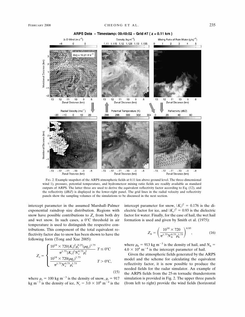
Given the atmospheric fields generated by the ARPSmodel and the scheme for calculating the equivalentreflectivity factor, it is now possible to produce theneeded fields for the radar simulator. An example ofthe ARPS fields from the 25-m tornadic thunderstormsimulation is provided in Fig. 2. The upper three panels(from left to right) provide the wind fields (horizontal

FIG. 2. Example snapshot of the ARPS atmospheric fields at 0.11 km above ground level. The three-dimensionalwind 1), pressure, potential temperature, and hydrometeor mixing ratio fields are readily available as standardoutputs of ARPS. The latter three are used to derive the equivalent reflectivity factor according to Eq. (12), andthe reflectivity (dBZ) is displayed in the lower-right panel. The grid lines in the radial velocity and reflectivitypanels show the sampling volumes of the simulations to be discussed in the next section.


wind vectors plus vertical velocity in shades), air den-sity, and rainwater mixing ratio, respectively. Assuminga simulated radar position to the right of the displayedfields, the radial velocity (Fig. 2d) is derived from thethree-dimensional wind by simple projection. The po-tential temperature is shown in Fig 2e. Equivalent re-flectivity factor derived from the ARPS fields is shownin Fig. 2f. Note that even though our reflectivity simu-lation can handle the effect of ice species, our currentdataset does not contain ice. As expected, regions ofhigh Ze follow regions with high rainwater mixing ratio.These fields are used in Eq. (1) to produce time seriesdata. Therefore, we will consider the data in Fig. 2 asground truth, with the resolution provided by the in-herent grid spacing of the ARPS output.

3. Quad-linear spatial and temporal interpolation

The atmospheric fields, which control the flow anddictate the characteristics of the scatterers, are typicallygenerated separately from the actual radar simulation.In other words, the pregenerated atmospheric fields donot directly affect the algorithmic flow of the simula-tion. Given the input fields, it is essential to grid thedata with a format that can be readily fed into the simu-lator. For efficiency, a lookup procedure and linear in-terpolation are used to extract the atmospheric param-eters corresponding to individual discrete scatterers(Cheong et al. 2004a). Using this technique, the simu-lator has the flexibility to incorporate atmosphericfields previously generated by a variety of models.

Therefore, it is not necessary to regenerate the fieldsfor each run of the simulator.

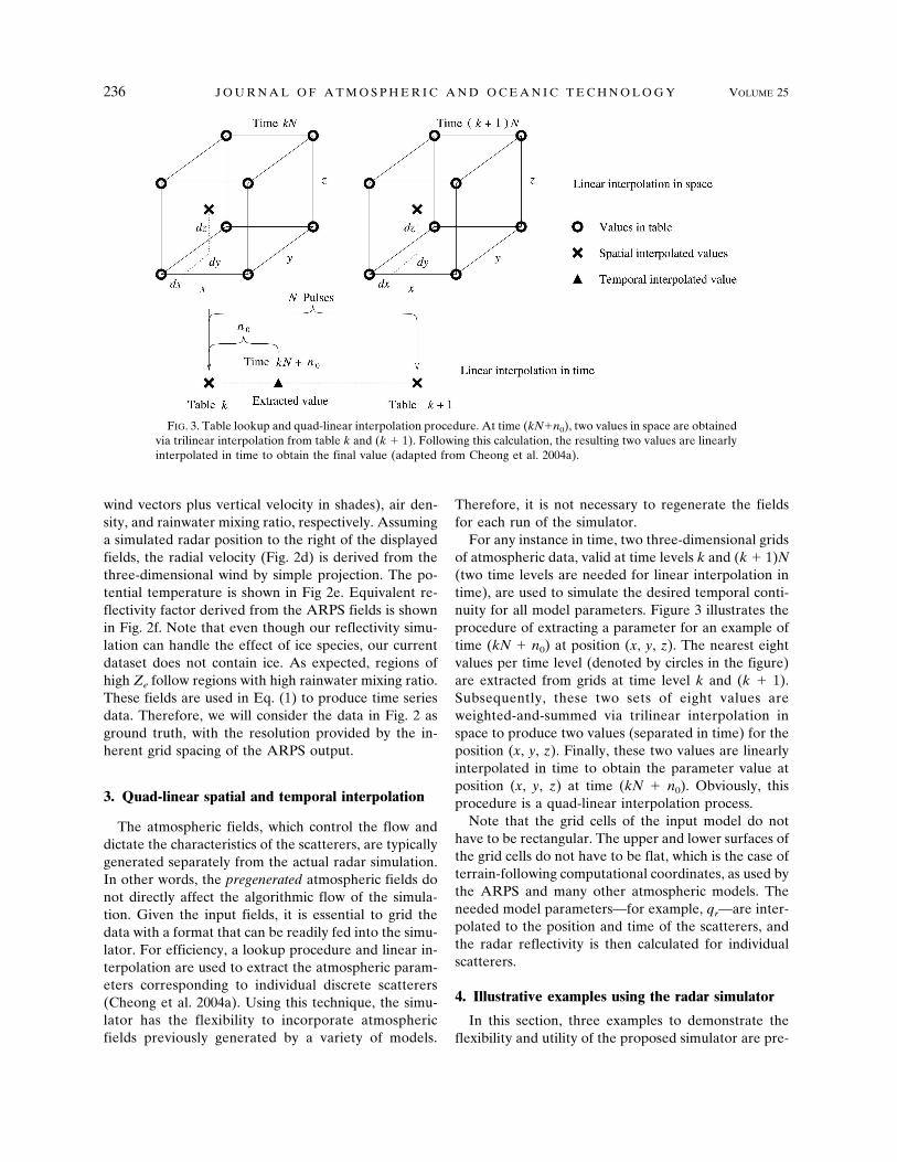
For any instance in time, two three-dimensional gridsof atmospheric data, valid at time levels k and (k � 1)N(two time levels are needed for linear interpolation intime), are used to simulate the desired temporal conti-nuity for all model parameters. Figure 3 illustrates theprocedure of extracting a parameter for an example oftime (kN � n0) at position (x, y, z). The nearest eightvalues per time level (denoted by circles in the figure)are extracted from grids at time level k and (k � 1).Subsequently, these two sets of eight values areweighted-and-summed via trilinear interpolation inspace to produce two values (separated in time) for theposition (x, y, z). Finally, these two values are linearlyinterpolated in time to obtain the parameter value atposition (x, y, z) at time (kN � n0). Obviously, thisprocedure is a quad-linear interpolation process.

Note that the grid cells of the input model do nothave to be rectangular. The upper and lower surfaces ofthe grid cells do not have to be flat, which is the case ofterrain-following computational coordinates, as used bythe ARPS and many other atmospheric models. Theneeded model parameters—for example, qr—are inter-polated to the position and time of the scatterers, andthe radar reflectivity is then calculated for individualscatterers.

4. Illustrative examples using the radar simulator

In this section, three examples to demonstrate theflexibility and utility of the proposed simulator are pre-

FIG. 3. Table lookup and quad-linear interpolation procedure. At time (kN�n0), two values in space are obtainedvia trilinear interpolation from table k and (k � 1). Following this calculation, the resulting two values are linearlyinterpolated in time to obtain the final value (adapted from Cheong et al. 2004a).


sented. As discussed previously, the radar simulatoruses Monte Carlo integration to emulate volume scat-tering. Because of the inherent sampling process, it isimportant that the number of scatterers be sufficientlylarge. By balancing adequate sampling of the desiredatmospheric features and computational cost, a generalrule has been determined that each simulated resolu-tion volume (gridded region in Fig. 2) should contain atleast 20 scatterers.

For a range of r, an approximation of the size of theresolution volume is given by

�V � r2��r�, �17�

where �� and �� represent the two angular beam-widths of the antenna in azimuth and elevation, respec-tively. This approximation will be used later to deter-mine the required number of scatterers for each simu-lation.

a. Single range gate canonical example

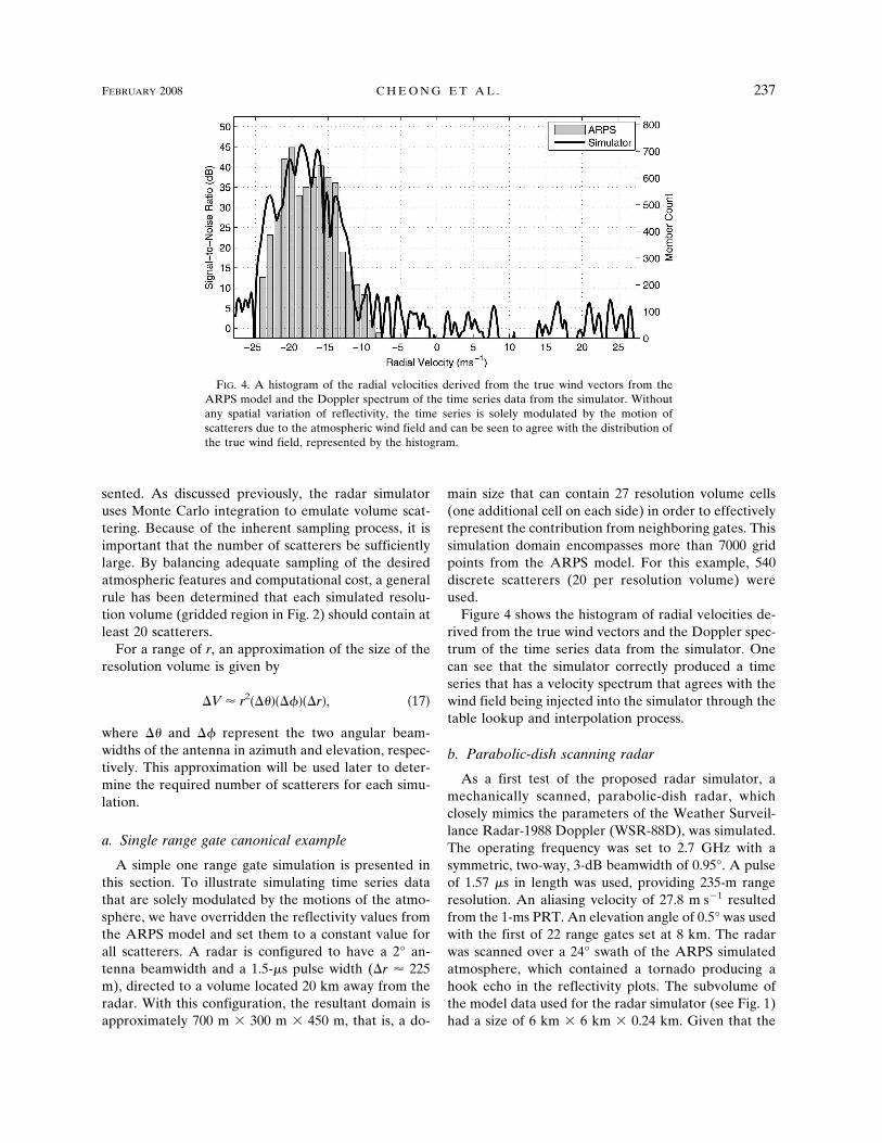
A simple one range gate simulation is presented inthis section. To illustrate simulating time series datathat are solely modulated by the motions of the atmo-sphere, we have overridden the reflectivity values fromthe ARPS model and set them to a constant value forall scatterers. A radar is configured to have a 2° an-tenna beamwidth and a 1.5-�s pulse width (�r � 225m), directed to a volume located 20 km away from theradar. With this configuration, the resultant domain isapproximately 700 m � 300 m � 450 m, that is, a do-

main size that can contain 27 resolution volume cells(one additional cell on each side) in order to effectivelyrepresent the contribution from neighboring gates. Thissimulation domain encompasses more than 7000 gridpoints from the ARPS model. For this example, 540discrete scatterers (20 per resolution volume) wereused.

Figure 4 shows the histogram of radial velocities de-rived from the true wind vectors and the Doppler spec-trum of the time series data from the simulator. Onecan see that the simulator correctly produced a timeseries that has a velocity spectrum that agrees with thewind field being injected into the simulator through thetable lookup and interpolation process.

b. Parabolic-dish scanning radar

As a first test of the proposed radar simulator, amechanically scanned, parabolic-dish radar, whichclosely mimics the parameters of the Weather Surveil-lance Radar-1988 Doppler (WSR-88D), was simulated.The operating frequency was set to 2.7 GHz with asymmetric, two-way, 3-dB beamwidth of 0.95°. A pulseof 1.57 �s in length was used, providing 235-m rangeresolution. An aliasing velocity of 27.8 m s�1 resultedfrom the 1-ms PRT. An elevation angle of 0.5° was usedwith the first of 22 range gates set at 8 km. The radarwas scanned over a 24° swath of the ARPS simulatedatmosphere, which contained a tornado producing ahook echo in the reflectivity plots. The subvolume ofthe model data used for the radar simulator (see Fig. 1)had a size of 6 km � 6 km � 0.24 km. Given that the

FIG. 4. A histogram of the radial velocities derived from the true wind vectors from theARPS model and the Doppler spectrum of the time series data from the simulator. Withoutany spatial variation of reflectivity, the time series is solely modulated by the motion ofscatterers due to the atmospheric wind field and can be seen to agree with the distribution ofthe true wind field, represented by the histogram.


resolution volume at 10 km (middle of the domain) isapproximately 6.46 � 106 m3, at least 2.67 � 104 scat-terers are needed in order to meet the aforementionedcondition of 20 scatterers per resolution volume. There-fore, 30 000 discrete scatterers were used for this ex-ample. The radar was scanned over the 24° angularregion with a 1° azimuthal sampling interval, althoughfiner sampling could easily be achieved. The antennarotation rate was set to produce 50 samples for eachazimuth angle with a 50-ms dwell time. Gaussian-distributed, complex noise was added to the time seriesdata in order to simulate electronic receiver noise.Since the noise floor should be approximately constantfor a particular radar system, the additive noise powerwas chosen to produce an average signal-to-noise ratio(SNR) of 70 dB over the entire domain (azimuth anglesand range) scanned by the radar.

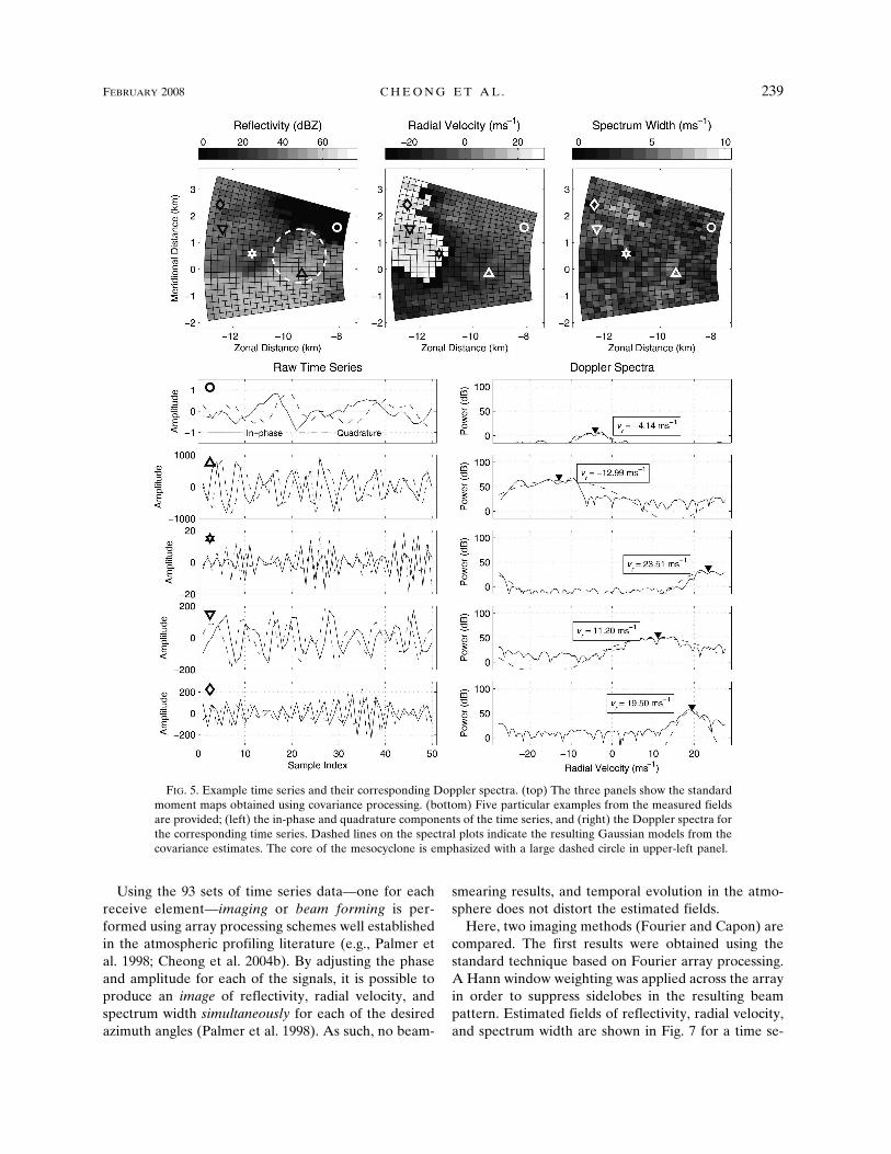
Using the 50 time series samples, the autocorrelationfunction at lags 0, 1, and 2 were estimated for eachrange gate and azimuth angle. These results were usedwith covariance processing to produce estimates of re-flectivity, radial velocity, and spectrum width, which areshown in the top three panels of Fig. 5. The simulatedradar is located to the right of the figure, which de-termined the orientation of the radial velocity. Thelimits of plot axes indicate the size of the input data gridor enclosing volume. As can be seen, the enclosing vol-ume is larger than the actual simulated region, whichmitigates artifacts caused by boundary effects as scat-terers enter/exit the volume (Holdsworth and Reid1995).

Markers on the moment fields indicate the locations,for which time series and corresponding Doppler spec-tral estimates are shown at the bottom of the figure.Five examples were chosen to sample a variety of at-mospheric conditions. The first example (denoted by acircle) corresponds to an extremely low-SNR case withthe expected flat spectral shape. The time series showlow-amplitude fluctuations typical of noise-dominatedsignals. Note that the axis scales for the time series plotsare not constant. The next example (denoted by a tri-angle) has the strongest backscattered power from theset and shows an inbound velocity of approximately�11.78 m s�1. The reflectivity is over 60 dBZ near thecore of the mesocyclone as indicated by large dashedcircle in upper-left panel. The last three examples pro-vide illustrations of partial aliasing, due to the 27.8m s�1 unambiguous velocity and various reflectivitylevels. In general, the estimated Doppler spectra have ashape (Gaussian) that is expected from volume-filledatmospheric scatter, lending credibility to the MonteCarlo integration scheme used.

c. Phased array imaging radar

As another example of the utility of the radar simu-lator, a more advanced radar design is now used. Here,a phased array radar system has been simulated with atransmit frequency of 3.2 GHz, a pulse width of 1.57 �s(�r � 235 m), and a PRT of 1 ms. The radar is scanningat an elevation angle of 1.5° at a range of 10 km for thefirst gate. Twenty-two (22) range gates are used with an18° azimuthal coverage (0.75° sampling) to observe thecyclonic circulation present in the ARPS data. To testaircraft clutter mitigation using adaptive beam formingand to illustrate the flexibility of the radar simulator, astrong point target (aircraft) has been inserted into theatmospheric fields of the ARPS model, flying towardthe northeast within the field of view, at a speed of 28m s�1. For simplicity, the reflectivity of the aircraft hasbeen chosen to be an arbitrarily high value of 80 dBZ inorder to have a target that obscures the weather signals.The enclosing volume for this simulation is approxi-mately 6 km � 5.2 km � 0.5 km.

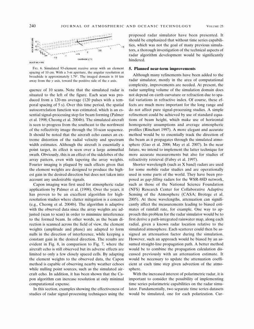
The simulated radar uses a spoiled transmit beamthat has a uniform 18° azimuth coverage. In practice,this can be accomplished by either using a subset oftransmit elements that is closer to the center of thearray, or an independent transmitter that has a widebeam pattern. In elevation, the transmit beam has abeamwidth (��) of 1.5° with a Gaussian weighting ap-plied so that scatterers on the scanning elevation planecontribute most significantly. Such a radar design willallow the scanned region to be simultaneously observedfrom all directions. The 93 receive elements of the arrayare shown in Fig. 6 and are assumed to be omnidirec-tional. In this case of an imaging radar, the simulatorwill produce time series data for each of the receiveelements. The azimuthal resolution can be estimatedusing (Stoica and Moses 1997)

�� sin�1� 1L�, �18�

where L � (m � 1)d/� is the array length measured inwavelengths, m is the number of elements across thelongest aperture, that is, m � 31, and d is the elementspacing, which is 10 cm for this particular configuration.The azimuthal angular resolution (�� ) is therefore ap-proximately 1.79°. Using a similar procedure to the pre-vious example to calculate the average number of scat-terers for the closest range gate and assuming that theelevation weighting limits the resolution volume as�� 1.5°, �V � r2(��)(�� )(�r) � 1.92 � 107 m3.Therefore, at least 1.62 � 104 discrete scatterers areneeded for proper sampling. The number of scattererswas set to 20 000 to provide some margin of error.


Using the 93 sets of time series data—one for eachreceive element—imaging or beam forming is per-formed using array processing schemes well establishedin the atmospheric profiling literature (e.g., Palmer etal. 1998; Cheong et al. 2004b). By adjusting the phaseand amplitude for each of the signals, it is possible toproduce an image of reflectivity, radial velocity, andspectrum width simultaneously for each of the desiredazimuth angles (Palmer et al. 1998). As such, no beam-

smearing results, and temporal evolution in the atmo-sphere does not distort the estimated fields.

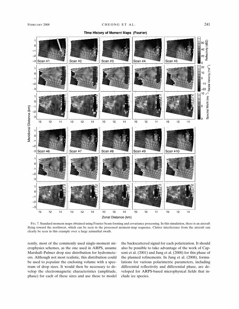
Here, two imaging methods (Fourier and Capon) arecompared. The first results were obtained using thestandard technique based on Fourier array processing.A Hann window weighting was applied across the arrayin order to suppress sidelobes in the resulting beampattern. Estimated fields of reflectivity, radial velocity,and spectrum width are shown in Fig. 7 for a time se-

FIG. 5. Example time series and their corresponding Doppler spectra. (top) The three panels show the standardmoment maps obtained using covariance processing. (bottom) Five particular examples from the measured fieldsare provided; (left) the in-phase and quadrature components of the time series, and (right) the Doppler spectra forthe corresponding time series. Dashed lines on the spectral plots indicate the resulting Gaussian models from thecovariance estimates. The core of the mesocyclone is emphasized with a large dashed circle in upper-left panel.


quence of 10 scans. Note that the simulated radar issituated to the left of the figure. Each scan was pro-duced from a 120-ms average (120 pulses with a tem-poral spacing of 5 s). Over this time period, the spatialautocorrelation function was estimated, which is an es-sential signal-processing step for beam forming (Palmeret al. 1998; Cheong et al. 2004b). The simulated aircraftis seen to progress from the southeast to the northwestof the reflectivity image through the 10-scan sequence.It should be noted that the aircraft echo causes an ex-treme distortion of the radial velocity and spectrumwidth estimates. Although the aircraft is essentially apoint target, its effect is seen over a large azimuthalswath. Obviously, this is an effect of the sidelobes of thearray pattern, even with tapering the array weights.Fourier imaging is plagued by such effects given thatthe element weights are designed to produce the high-est gain in the desired direction but does not taken intoaccount any undesirable signals.

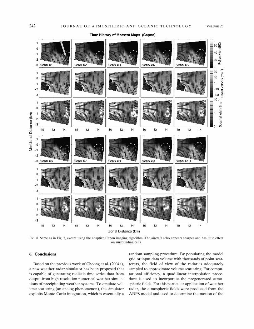
Capon imaging was first used for atmospheric radarapplications by Palmer et al. (1998). Over the years, ithas proven to be an excellent algorithm for high-resolution studies where clutter mitigation is a concern(e.g., Cheong et al. 2004b). The algorithm is adaptivewith the observed data since the array weights are ad-justed (scan to scan) in order to minimize interferenceto the formed beam. In other words, as the beam di-rection is scanned across the field of view, the elementweights (amplitude and phase) are adapted to formnulls in the direction of interference, while keeping aconstant gain in the desired direction. The results areevident in Fig. 8, in comparison to Fig. 7, where theaircraft echo is still observed but its adverse effects arelimited to only a few closely spaced cells. By adaptingthe element weights to the observed data, the Caponmethod is capable of observing nearby weather echoeswhile nulling point sources, such as the simulated air-craft echo. In addition, it has been shown that the Ca-pon algorithm can increase resolution at only minimalcomputational expense.

In this section, examples showing the effectiveness ofstudies of radar signal-processing techniques using the

proposed radar simulator have been presented. Itshould be emphasized that without time series capabili-ties, which was not the goal of many previous simula-tors, a thorough investigation of the technical aspects ofradar algorithm development would be significantlyhindered.

5. Planned near-term improvements

Although many refinements have been added to theradar simulator, mostly in the area of computationalcomplexity, improvements are needed. At present, theradar sampling volume of the simulation domain doesnot depend on earth curvature or refraction due to spa-tial variations in refractive index. Of course, these ef-fects are much more important for the long range anddo not affect pure signal-processing studies. A simplerefinement could be achieved by use of standard equa-tions of beam height, which make use of horizontalhomogeneity assumptions and average atmosphericprofiles (Rinehart 1997). A more elegant and accuratemethod would be to essentially track the direction ofthe beam as it propagates through the simulated atmo-sphere (Gao et al. 2006; May et al. 2007). In the nearfuture, we intend to implement the latter technique formore accurate measurements but also for studies ofrefractivity retrieval (Fabry et al. 1997).

Shorter wavelength (such as X band) radars are usedfor some mobile radar studies and are operationallyused in some parts of the world. They have been pro-posed as gap-filling radars for the WSR-88D network,such as those of the National Science Foundation(NFS) Research Center for Collaborative AdaptiveSensing of the Atmosphere (CASA; Brotzge et al.2005). At these wavelengths, attenuation can signifi-cantly affect the measurements leading to biased esti-mates of rainfall rate, for example. One way to ap-proach this problem for the radar simulator would be tofirst derive a path-integrated rainwater map, along eachradial, given a known radar location relative to thesimulated atmosphere. Each scatterer could then be as-signed an attenuation factor during the simulation.However, such an approach would be biased by an as-sumed straight-line propagation path. A better methodwould be to combine the propagation calculation dis-cussed previously with an attenuation estimate. Itwould be necessary to update the attenuation coeffi-cient at each time step given advection of the atmo-sphere.

With the increased interest of polarimetric radar, it isimportant to consider the possibility of implementingtime series polarimetric capabilities on the radar simu-lator. Fundamentally, two separate time series datasetswould be simulated, one for each polarization. Cur-

FIG. 6. Simulated 93-element receive array with an elementspacing of 10 cm. With a 3-m aperture, the angular resolution atbroadside is approximately 1.79°. The imaged domain is 10 kmaway from the y axis, toward the positive side of the x axis.


rently, most of the commonly used single-moment mi-crophysics schemes, as the one used in ARPS, assumeMarshall–Palmer drop size distribution for hydromete-ors. Although not most realistic, this distribution couldbe used to populate the enclosing volume with a spec-trum of drop sizes. It would then be necessary to de-velop the electromagnetic characteristics (amplitude,phase) for each of these sizes and use these to model

the backscattered signal for each polarization. It shouldalso be possible to take advantage of the work of Cap-soni et al. (2001) and Jung et al. (2008) for this phase ofthe planned refinements. In Jung et al. (2008), formu-lations for various polarimetric parameters, includingdifferential reflectivity and differential phase, are de-veloped for ARPS-based microphysical fields that in-clude ice species.

FIG. 7. Standard moment maps obtained using Fourier beam forming and covariance processing. In this simulation, there is an aircraftflying toward the northwest, which can be seen in the processed moment-map sequence. Clutter interference from the aircraft canclearly be seen in this example over a large azimuthal swath.


6. Conclusions

Based on the previous work of Cheong et al. (2004a),a new weather radar simulator has been proposed thatis capable of generating realistic time series data fromoutput from high-resolution numerical weather simula-tions of precipitating weather systems. To emulate vol-ume scattering (an analog phenomenon), the simulatorexploits Monte Carlo integration, which is essentially a

random sampling procedure. By populating the modelgrid or input data volume with thousands of point scat-terers, the field of view of the radar is adequatelysampled to approximate volume scattering. For compu-tational efficiency, a quad-linear interpolation proce-dure is used to incorporate the pregenerated atmo-spheric fields. For this particular application of weatherradar, the atmospheric fields were produced from theARPS model and used to determine the motion of the

FIG. 8. Same as in Fig. 7, except using the adaptive Capon imaging algorithm. The aircraft echo appears sharper and has little effecton surrounding cells.


point scatterers and their reflectivity. Two exampleswere provided to illustrate the flexibility and capabili-ties of the simulator. First, a radar system similar to ascanning WSR-88D was investigated. Time series dataand their corresponding Doppler spectra were gener-ated for a variety of locations within the data grid. Itwas evident that realistic radar data were generated.Second, an advanced imaging radar was simulated,where a wide transmit beam was used with 93 indepen-dent receiving elements. By array processing (beamforming or imaging), it was possible to simultaneouslyimage the radar field of view. Advantages for suchphased array systems, in addition to the overall useful-ness of the proposed radar simulator, will be investi-gated in future publications.

Acknowledgments. This work was partially supportedby the National Severe Storms Laboratory (NOAA/NSSL) under Cooperative Agreement NA17RJ1227.Ming Xue was also supported by NFS Grants EEC-0313747 and ATM-0530814.

REFERENCES

Anagnostou, E. N., and W. F. Krajewski, 1997: Simulation of ra-dar reflectivity fields: Algorithm formulation and evaluation.Water Resour. Res., 33, 1419–1428.

Brotzge, J. A., K. Brewster, B. Johnson, B. Philips, M. Preston, D.Westbrook, and M. Zink, 2005: CASA’s first test bed: Inte-grative Project #1. Preprints, 32nd Conf. on Radar Meteorol-ogy, Albuquerque, NM, Amer. Meteor. Soc., 14R.2.

Capsoni, C., and M. D’Amico, 1998: A physically based radarsimulator. J. Atmos. Oceanic Technol., 15, 593–598.

——, ——, and R. Nebuloni, 2001: A multiparameter polarimetricradar simulator. J. Atmos. Oceanic Technol., 18, 1799–1809.

Caumont, O., and Coauthors, 2006: A radar simulator for high-resolution nonhydrostatic models. J. Atmos. Oceanic Tech-nol., 23, 1049–1067.

Chandrasekar, V., and V. N. Bringi, 1987: Simulation of radarreflectivity and surface measurements of rainfall. J. Atmos.Oceanic Technol., 4, 464–478.

Cheong, B. L., M. W. Hoffman, and R. D. Palmer, 2004a: Effi-cient atmospheric simulation for high-resolution radar imag-ing applications. J. Atmos. Oceanic Technol., 21, 374–378.

——, ——, ——, S. J. Frasier, and F. J. López-Dekker, 2004b:Pulse pair beamforming and the effects of reflectivity fieldvariations on imaging radars. Radio Sci., 39, RS3014,doi:10.1029/2002RS002843.

Doviak, R. J., and D. S. Zrnic, 1993: Doppler Radar and WeatherObservations. 2nd ed. Academic Press, 562 pp.

Fabry, F., C. Frush, I. Zawadzki, and A. Kilambi, 1997: On theextraction of near-surface index of refraction using radarphase measurements from ground targets. J. Atmos. OceanicTechnol., 14, 978–987.

Gao, J., K. Brewster, and M. Xue, 2006: A comparison of theradar ray path equations and approximations for use in radardata assimilations. Adv. Atmos. Sci., 23, 190–198.

Holdsworth, D. A., and I. M. Reid, 1995: A simple model of at-mospheric radar backscatter: Description and application to

the full correlation analysis of spaced antenna data. RadioSci., 30, 1263–1280.

Jung, Y., M. Xue, G. Zhang, and J. Straka, 2008: Assimilation ofsimulated polarimetric radar data for a convective storm us-ing ensemble Kalman filter. Part I: Observation operators forreflectivity and polarimetric variables. Mon. Wea. Rev., inpress.

Krajewski, W. F., R. Raghavan, and V. Chandrasekar, 1993:Physically based simulation of radar rainfall data using aspace–time rainfall model. J. Appl. Meteor., 32, 268–283.

Liu, S., M. Xue, and Q. Xu, 2007: Using wavelet analysis to detecttornadoes from Doppler radar radial-velocity observations. J.Atmos. Oceanic Technol., 24, 344–359.

Marshall, J. S., and W. M. Palmer, 1948: The distribution of rain-drops with size. J. Meteor., 5, 165–166.

May, R. M., M. I. Biggerstaff, and M. Xue, 2007: A Doppler radaremulator with an application to the detectability of tornadicsignatures. J. Atmos. Oceanic Technol., 24, 1973–1996.

Metropolis, N., and S. Ulam, 1949: The Monte Carlo method. J.Amer. Stat. Assoc., 44, 335–341.

Palmer, R. D., S. Gopalam, T. Yu, and S. Fukao, 1998: Coherentradar imaging using Capon’s method. Radio Sci., 33, 1585–1598.

Ray, P. S., B. C. Johnson, K. W. Johnson, J. S. Bradberry, J. J.Stephens, K. K. Wagner, and J. B. Klemp, 1981: The mor-phology of severe tornadic storms on 20 May 1997. J. Atmos.Sci., 38, 1643–1663.

Rinehart, R. E., 1997: Radar for Meteorologists. 3rd ed. RinehartPublications, 482 pp.

Smith, P. L., Jr., C. G. Myers, and H. D. Orville, 1975: Radar re-flectivity factor calculations in numerical cloud models usingbulk parameterization of precipitation. J. Appl. Meteor., 14,1156–1165.

Stoica, P., and R. Moses, 1997: Introduction to Spectral Analysis.Prentice-Hall, 319 pp.

Tong, M., and M. Xue, 2005: Ensemble Kalman filter assimilationof Doppler radar data with a compressible nonhydrostaticmodel: OSS experiments. Mon. Wea. Rev., 133, 1789–1807.

Ulbrich, C. W., 1983: Natural variations in the analytical form ofraindrop size distribution. J. Climate Appl. Meteor., 22, 1764–1775.

Xue, M., K. K. Droegemeier, and V. Wong, 2000: The AdvancedRegional Prediction System (ARPS)—A multiscale nonhy-drostatic atmospheric simulation and prediction tool. Part I:Model dynamics and verification. Meteor. Atmos. Phys., 75,161–193.

——, and Coauthors, 2001: The Advanced Regional PredictionSystem (ARPS)—A multiscale nonhydrostatic atmosphericsimulation and prediction tool. Part II: Model physics andapplications. Meteor. Atmos. Phys., 76, 143–165.

——, D.-H. Wang, J.-D. Gao, K. Brewster, and K. K. Droege-meier, 2003: The Advanced Regional Prediction System(ARPS), storm-scale numerical weather prediction and dataassimilation. Meteor. Atmos. Phys., 82, 139–170.

——, S. Liu, and T. Yu, 2007: Variational analysis of oversampleddual-Doppler radial velocity data and application to theanalysis of tornado circulations. J. Atmos. Oceanic Technol.,24, 403–414.

Yu, T.-Y., R. D. Palmer, and D. L. Hysell, 2000: A simulationstudy of coherent radar imaging. Radio Sci., 35, 1129–1141.

Zrnic, D. S., 1975: Simulation of weatherlike Doppler spectra andsignals. J. Appl. Meteor., 14, 619–620.


Documents

A Time Series Weather Radar Simulator Based on High