Embed Size (px)
Citation preview

i
A Three-Dimensional Ray Tracing Simulation of a Synthetic Aperture
Ground Penetrating Radar System
By
James W. Jeter III
A Thesis Submitted
in Partial Fulfillment of the
Requirements for the Degree of
MASTER OF SCIENCE
In
Electrical Engineering
Approved by theThesis Committee:
____________________________Dr. Vincent J. Amuso, Thesis Adviser
___________________________Dr. Sohail A. Dianat, Member
___________________________Dr. Raghuveer Rao, Member
___________________________Dr. John Schott, Member
___________________________Dr. Robert J. Bowman, Department Chairman
Rochester Institute of TechnologyRochester, New York
August 2002

Report Documentation Page
Report Date 04OCT2002
Report Type N/A
Dates Covered (from... to) -
Title and Subtitle A Three-Dimensional Ray Tracing Simulation of aSynthetic Aperture Ground Penetrating Radar System
Contract Number
Grant Number
Program Element Number
Author(s) Jeter III, James W.
Project Number
Task Number
Work Unit Number
Performing Organization Name(s) and Address(es) Rochester Institute of Technology
Performing Organization Report Number
Sponsoring/Monitoring Agency Name(s) and Address(es) The Department of the Air Force AFIT/CIA, Bldg. 1252950 P Street Wright-Patterson AFB, OH 45433
Sponsor/Monitor’s Acronym(s)
Sponsor/Monitor’s Report Number(s)
Distribution/Availability Statement Approved for public release, distribution unlimited
Supplementary Notes
Abstract
Subject Terms
Report Classification unclassified
Classification of this page unclassified
Classification of Abstract unclassified
Limitation of Abstract UU
Number of Pages 145

ii
The views expressed in this thesis are those of the author and do notreflect the official policy or position of the United States Air Force, Departmentof Defense, or the U.S. Government.
I, James W. Jeter III, hereby grant permission to the Wallace Library ofthe Rochester Institute of Technology to reproduce my thesis in whole or in part.Any reproduction will not be for commercial use or profit.
Date:__________________ Signature of Author:______________________________

iii
Table of Contents
TABLE OF CONTENTS........................................................................................................................................... III
LIST OF TABLES .........................................................................................................................................................V
LIST OF FIGURES .................................................................................................................................................... VI
ACKNOWLEDGMENTS ......................................................................................................................................VIII
ABSTRACT.................................................................................................................................................................. IX
CHAPTER 1 ....................................................................................................................................................................1
INTRODUCTION .............................................................................................................................................................11.1 Problem Statement ...........................................................................................................................................11.2 Overview.............................................................................................................................................................2
CHAPTER 2 ....................................................................................................................................................................4
REVIEW OF LITERATURE ..............................................................................................................................................42.1 Finite Difference, Time Domain Technique.................................................................................................42.2 Ray-Tracing Technique ...................................................................................................................................9
CHAPTER 3 ................................................................................................................................................................. 14
THEORY........................................................................................................................................................................143.1 Electromagnetic Waves................................................................................................................................. 143.2 Electromagnetic Fields................................................................................................................................. 173.3 Antenna Reflection Characteristics............................................................................................................ 193.4 Physical and Geometrical Models.............................................................................................................. 203.5 Antenna Beam Forming................................................................................................................................ 253.6 Attenuation...................................................................................................................................................... 273.7 Radar ............................................................................................................................................................... 32
CHAPTER 4 ................................................................................................................................................................. 35
EXPERIMENTAL IMPLEMENTATION ..........................................................................................................................354.1 Surface Generation ....................................................................................................................................... 354.2 Ray Generation.............................................................................................................................................. 374.3 Intersection Detection................................................................................................................................... 394.4 Reflected and Transmitted Ray Calculation ............................................................................................. 484.5 Attenuation...................................................................................................................................................... 534.6 Synthetic Return Generation ....................................................................................................................... 554.7 Automatic Ray Generation........................................................................................................................... 55
CHAPTER 5 ................................................................................................................................................................. 59
DESCRIPTION OF SYSTEM..........................................................................................................................................595.1 Transmission and Reception........................................................................................................................ 595.2 Pre-Processing............................................................................................................................................... 625.3 SAR Processing.............................................................................................................................................. 665.4 GPR Simulation ............................................................................................................................................. 69
CHAPTER 6 ................................................................................................................................................................. 73
RESULTS.......................................................................................................................................................................73

iv
6.1 Automatic Ray Generation........................................................................................................................... 746.1.1 Transmitter Orientation...............................................................................................................................766.1.2 Receiver Orientation....................................................................................................................................80
6.2 Manually Generated Rays............................................................................................................................ 886.2.1 Target Position ............................................................................................................................................936.2.2 Resolution / Number of Rays....................................................................................................................102
6.3 Uniform Point Scatterer Simulation.........................................................................................................110
CHAPTER 7 ...............................................................................................................................................................114
DISCUSSION ...............................................................................................................................................................1147.1 Automatic Ray Generation.........................................................................................................................117
7.1.1 Transmitter Orientation.............................................................................................................................1197.1.2 Receiver Orientation..................................................................................................................................119
7.2 Manually Generated Rays..........................................................................................................................1227.2.1 Target Position ..........................................................................................................................................1237.2.2 Resolution / Number of Rays....................................................................................................................126
7.3 Uniform Point Scatterer Simulation.........................................................................................................127
CHAPTER 8 ...............................................................................................................................................................129
CONCLUSIONS............................................................................................................................................................1298.1 Simulation.....................................................................................................................................................1298.2 Assessment of Ray-Tracing Effects ...........................................................................................................1298.3 Future Work..................................................................................................................................................131
BIBLIOGRAPHY AND CITATION INDEX....................................................................................................133

v
List of Tables
TABLE 4.1 FACET DATA TABLE.....................................................................................................................................37TABLE 6.1 DATA SET 1 SCENE CONFIGURATION INFORMATION.............................................................................75TABLE 6.2 DATA SET 2 SCENE CONFIGURATION INFORMATION.............................................................................77TABLE 6.3 DATA SET 3 SCENE CONFIGURATION INFORMATION.............................................................................79TABLE 6.4 DATA SET 4 SCENE CONFIGURATION INFORMATION.............................................................................81TABLE 6.5 DATA SET 5 SCENE CONFIGURATION INFORMATION.............................................................................83TABLE 6.6 DATA SET 6 SCENE CONFIGURATION INFORMATION.............................................................................85TABLE 6.7 DATA SET 7 SCENE CONFIGURATION INFORMATION.............................................................................87TABLE 6.8 DATA SET 8 SCENE CONFIGURATION INFORMATION.............................................................................91TABLE 6.9 DATA SET 9 SCENE CONFIGURATION INFORMATION.............................................................................93TABLE 6.10 DATA SET 10 SCENE CONFIGURATION INFORMATION ........................................................................95TABLE 6.11DATA SET 11 SCENE CONFIGURATION INFORMATION .........................................................................97TABLE 6.12 DATA SET 12 SCENE CONFIGURATION INFORMATION ........................................................................99TABLE 6.13 DATA SET 13 SCENE CONFIGURATION INFORMATION ......................................................................101TABLE 6.14 DATA SET 14 SCENE CONFIGURATION INFORMATION ......................................................................103TABLE 6.15 DATA SET 15 SCENE CONFIGURATION INFORMATION ......................................................................105TABLE 6.16 DATA SET 16 SCENE CONFIGURATION INFORMATION ......................................................................107TABLE 6.17 DATA SET 17 SCENE CONFIGURATION INFORMATION ......................................................................109

vi
List of Figures
FIGURE 2.1: YEE CUBE...................................................................................................................................................5FIGURE 3.1: ELECTRIC AND MAGNETIC FIELD COMPONENTS OF AN EM WAVE...............................................17FIGURE 3.2: FEYNMAN'S QED ANALYSIS OF REFLECTION....................................................................................22FIGURE 3.3: SNELL'S LAW DEFINITION DIAGRAM..................................................................................................24FIGURE 3.4: ANTENNA BEAM PATTERN ....................................................................................................................27FIGURE 4.1: TRANSMITTED RAY ORIENTATION.....................................................................................................39FIGURE 4.2: COLLAPSED FACET DIAGRAM..............................................................................................................41FIGURE 4.3: VALID INTERSECTION DETERMINATION...........................................................................................43FIGURE 4.4: PROJECTED FACET IN X-Y DIMENSION..............................................................................................44FIGURE 4.5: INVALID INTERSECTION LINE EXAMPLES ..........................................................................................46FIGURE 4.6: LAW OF REFLECTION ............................................................................................................................49FIGURE 4.7: TRANSMITTED RAY CALCULATION DIAGRAM.................................................................................51FIGURE 4.8: AUTOMATIC RAY GENERATION EXAMPLE.........................................................................................56FIGURE 5.1: ROME LABS GPR CONFIGURATION.....................................................................................................59FIGURE 5.2: ROME LABS TRANSMITTER AND RECEIVER SYSTEM .......................................................................60FIGURE 5.3: ROME LABS PRE-PROCESSING SYSTEM ...............................................................................................62FIGURE 5.4-A: A TIME WINDOWEDSINUSOID...........................................................................................................65FIGURE 5.4-B: HANNING FILTER]...............................................................................................................................66FIGURE 5.4-C: HANNING FILTER ASSIGNED TO WINDOWED SIGNAL..................................................................66FIGURE 5.5: ROME LABS SAR PROCESSING SYSTEM...............................................................................................67FIGURE 6.1-A: DATA SET 1 SCENE CONFIGURATION IMAGE................................................................................75FIGURE 6.1-B: DATA SET 1 GPR PROCESSED IMAGE..............................................................................................76FIGURE 6.2-A: DATA SET 2 SCENE CONFIGURATION IMAGE................................................................................77FIGURE 6.2-B: DATA SET 2 GPR PROCESSED IMAGE..............................................................................................78FIGURE 6.3-A: DATA SET 3 SCENE CONFIGURATION IMAGE................................................................................79FIGURE 6.3-B: DATA SET 3 GPR PROCESSED IMAGE..............................................................................................80FIGURE 6.4-A: DATA SET 4 SCENE CONFIGURATION IMAGE................................................................................81FIGURE 6.4-B: DATA SET 4 GPR PROCESSED IMAGE..............................................................................................82FIGURE 6.5-A: DATA SET 5 SCENE CONFIGURATION IMAGE................................................................................83FIGURE 6.5-B: DATA SET 5 GPR PROCESSED IMAGE..............................................................................................84FIGURE 6.6-A: DATA SET 6 SCENE CONFIGURATION IMAGE................................................................................85FIGURE 6.6-B: DATA SET 6 GPR PROCESSED IMAGE..............................................................................................86FIGURE 6.7-A: DATA SET 7 SCENE CONFIGURATION IMAGE................................................................................87FIGURE 6.7-B: DATA SET 7 GPR PROCESSED IMAGE..............................................................................................88FIGURE 6.8-A: DATA SET 8 SCENE CONFIGURATION IMAGE................................................................................91FIGURE 6.8-B: DATA SET 8 GPR PROCESSED IMAGE..............................................................................................92FIGURE 6.9-A: DATA SET 9 SCENE CONFIGURATION IMAGE................................................................................93FIGURE 6.9-B: DATA SET 9 GPR PROCESSED IMAGE..............................................................................................94FIGURE 6.10-A: DATA SET 10 SCENE CONFIGURATION IMAGE............................................................................95FIGURE 6.10-B: DATA SET 10 GPR PROCESSED IMAGE..........................................................................................96FIGURE 6.11-A: DATA SET 11 SCENE CONFIGURATION IMAGE............................................................................97FIGURE 6.11-B: DATA SET 11 GPR PROCESSED IMAGE..........................................................................................98FIGURE 6.12-A: DATA SET 12 SCENE CONFIGURATION IMAGE............................................................................99FIGURE 6.12-B: DATA SET 12 GPR PROCESSED IMAGE........................................................................................100FIGURE 6.13-A: DATA SET 13 SCENE CONFIGURATION IMAGE..........................................................................101FIGURE 6.13-B: DATA SET 13 GPR PROCESSED IMAGE........................................................................................102FIGURE 6.14-A: DATA SET 14 SCENE CONFIGURATION IMAGE..........................................................................103FIGURE 6.14-B: DATA SET 14 GPR PROCESSED IMAGE........................................................................................104FIGURE 6.15-A: DATA SET 15 SCENE CONFIGURATION IMAGE..........................................................................105FIGURE 6.15-B: DATA SET 15 GPR PROCESSED IMAGE........................................................................................106

vii
FIGURE 6.16-A: DATA SET 16 SCENE CONFIGURATION IMAGE..........................................................................107FIGURE 6.16-B: DATA SET 16 GPR PROCESSED IMAGE........................................................................................108FIGURE 6.17-A: DATA SET 17 SCENE CONFIGURATION IMAGE..........................................................................109FIGURE 6.17-B: DATA SET 17 GPR PROCESSED IMAGE........................................................................................110FIGURE 6.18: DATA SET 18 GPR PROCESSED IMAGE............................................................................................111FIGURE 6.19: DATA SET 19 GPR PROCESSED IMAGE............................................................................................112FIGURE 6.20: DATA SET 20 GPR PROCESSED IMAGE.............................................................................................113FIGURE 7.1: GPR PROCESSING AMBIGUITY ELLIPSE..........................................................................................114FIGURE 7.2: TWO DIMENSIONAL REPRESENTATION OF GPR PROCESSED IMAGE IN X DIMENSION............115FIGURE 7.3: TWO DIMENSIONAL REPRESENTATION OF GPR PROCESSED IMAGE IN Y DIMENSION ............116FIGURE 7.4: X AND Y ELLIPSE REPRESENTATION OF DATA SET 1 ......................................................................118FIGURE 7.5: X AND Y ELLIPSE REPRESENTATION OF DATA SET 4 ......................................................................119FIGURE 7.6: X AND Y ELLIPSE REPRESENTATION OF DATA SET 5 ......................................................................120FIGURE 7.7: X AND Y ELLIPSE REPRESENTATION OF DATA SET 6 ......................................................................121FIGURE 7.8: X AND Y ELLIPSE REPRESENTATION OF DATA SET 7 ......................................................................122FIGURE 7.9: X AND Y ELLIPSE REPRESENTATION OF DATA SET 13....................................................................126FIGURE 8.1: NEVADA TEST SITE EXAMPLE IMAGE.............................................................................................132

viii
ACKNOWLEDGEMENTS
I would like to thank my thesis committee, for providing input and suggestions
throughout the writing process. I would also like to thank Douglas Lynch, Russell
Brown, James VanDamme, Michael Wicks, and Al George for giving me the opportunity
to work with their system and offering their expertise in teaching me about it. I would
especially like to thank Dr. Amuso for being patient and keeping me on track. I couldn’t
have asked for a better advisor and I wish you the best of luck in future endeavors.
Finally, I would like to thank my parents, who through this, as with everything else, have
given me the strength, advice and support I needed.

ix
ABSTRACT
Ground Penetrating Radar (GPR) is a useful tool for imaging the area below the
Earth’s surface. GPR works on the same principle as traditional radar, evaluating the
electromagnetic returns reflected from an object or scene of interest to determine
characteristics of the object that reflected the signal. Synthetic Aperture Radar (SAR) is
a technique which combines radar returns of a given scene collected at several positions.
By compiling the information contained in the returns, an image of a scene can be
generated. Combining these two concepts allows us to create an image of an
underground scene.
Air Force Research Lab, Rome, NY developed a ground penetrating, SAR system
with a resolution of approximately three feet capable of penetrating to depths of 150-160
feet into the ground. In order to assess the results obtained from this system, a simulation
was needed to generate expected returns from a user-defined synthetic scene.
Ray-tracing is a simulation technique that is frequently used to model radar and imaging
systems. In the ray-tracing model, the transmitted radar signal is simulated by a number
of straight lines, or rays, which propagate through the scene according to the principles of
electromagnetic theory. The data carried with each ray can be used to generate a
simulated radar return at the receiver.
This thesis describes a ray-tracing simulator, which was created to work in
conjunction with the Rome Labs GPR system. The ray-tracing simulation models the
transmissions and reflections from faceted target models using Snell’s law and the Law

x
of Reflection. The results obtained demonstrate the effects that different scene
orientations have upon the images generated by the Rome Labs system.

1
1. Introduction
When finding a needle in a haystack, it is helpful to know what the needle looks
like. Ground penetrating radar data often resembles the proverbial haystack. A layer of
ground with an unknown physical makeup obscures the target of interest, making it
difficult to discern if the target is being observed, or simply another piece of hay. The
unknown nature of the underground environment adds uncertainty as to how a valid
return should look for a given target. The data received from a target of interest is often
cluttered with returns from other objects around it, making it hard to interpret. It is useful
to have a means to generate a controlled return that is created in a scene composed of
material whose properties and dimensions are known. The control return can be used to
aid in interpreting the received data or as a diagnostic tool for the GPR system.
Control return data can be generated either from a controlled test environment or
a simulated scene. A controlled test environment is difficult to create in a GPR
environment because it must be submerged underground and uncovered whenever
changes are made to the scene’s configuration. This technique is not only labor intensive,
but prone to errors caused by soil property inconsistency. It is useful to have a means of
accurately generating synthetic data based upon a simulated scene that can be easily
manipulated. A simulated return from a synthetic scene provides this needed capability.
1.1 Problem Statement
This thesis presents a simulator that was developed to be used with a GPR system
designed by Rome Labs. The Rome Labs GPR system employs synthetic aperture radar

2
to image an underground scene. A signal is transmitted from a single transmitter location
and measured at several receiver locations within a receiver array grid. From these
returns an image is generated in a simulated scene space. Rome Labs also developed a
simulator in conjunction with their GPR system. The Rome Labs simulator models
targets as ideal point reflectors that reflect equally to every receiver location in the
receiver array grid. While this technique provides diagnostic validation of the GPR
system, it does not provide the flexibility to accurately model the physical properties of
different antenna and targets in the scene. The objective for this thesis is to develop a
simulator that simulates complex targets, can accurately simulate the electromagnetic
properties of the transmitted signal, is easily modified for different scenes, and is easily
upgradeable.
1.2 Overview
The purpose of this thesis is to describe the implementation of a simulation
technique that improves upon the simulator designed by Rome Labs. The document is
organized as described below:
Chapter 1: Introduce the problem and define the bounds of the solution.
Chapter 2: Reviews works researched in the area of ground penetrating radar.
Chapter 3: Describes the background theory necessary to adequately describe the
simulation technique.
Chapter 4: Describes the simulation approach used.
Chapter 5: Discusses the Rome Labs ground penetrating radar processing system.

3
Chapter 6: Describes the experimental implementation of the GPR simulator and
discusses the results.
Chapter 7: Summarizes conclusions made through experimentation and discusses
potential future activities.

4
2. Review of Literature
It is considerably more difficult to model a ground penetrating radar system than
to model a similar system designed for use above ground. Simulations used in ground
penetrating radar must account for phenomena that can be neglected in above ground
radar simulators. The dielectric properties of the ground can be varied, which can cause
unwanted clutter or ambiguous returns. Attenuation limits the depth of ground
penetration and affects the frequencies that can be used. The limited depth of penetration
and frequency requirements can also force the radar to operate in the near field. The
simulation technique used needs to account for these constraints. Two techniques that are
frequently used to simulate GPR systems are the finite difference, time domain (FDTD)
technique and the ray-tracing technique.
2.1 Finite Difference, Time Domain Technique
Maxwell’s equations rely upon initial temporal and spatial boundary conditions to
calculate the magnitude of an electromagnetic field. In a heterogeneous dielectric
medium, the dielectric properties vary considerably making Maxwell’s equations difficult
to solve. The FDTD technique was proposed by Kane S. Yee in his 1965 paper
‘Numerical Solutions of Initial Boundary Value Problems Involving Maxwell’s
Equations in Isotropic Media’ to solve Maxwell’s equations sequentially. Yee divides
the region of interest into a number of small cubic regions, using a discrete approach to
evaluate Maxwell’s equations at many points throughout the scene. Boundary conditions

5
for these regions are first defined and Maxwell’s equations are then solved sequentially
for each cube.
The first step in the FDTD technique involves dividing the region of interest into
a grid of cubic regions (see Figure 2.1). These cubes will be referred to as cells. The
dimensions of each cell in the grid must be a fraction of the wavelength of the transmitted
signal [1]. Boundary conditions are then defined for each cell in the grid. Yee assumes
the conducting surface to be a perfectly conducting surface and limits his calculations to
the transverse magnetic field case, where the magnetic component of the electromagnetic
field is parallel to the
Figure 2.1: Yee Cube
surface. The tangential components of the electric field and the normal component of the
magnetic field are therefore both zero. By using the X,Y, and Z directional components
of Maxwell’s equations, the electromagnetic field can be evaluated sequentially along all

6
of the discrete borders of the cells in the target scene. These modified versions of
Maxwell’s equations can be used to derive finite difference equations at the discrete cube
boundaries for the transverse electric (TE) field and transverse magnetic (TM) field
cases. [1]
TE case:
[ ]
[ ]
[ ]
[ ]0.)
)2/1,2/1()2/1,2/1()2/1,(.)
)2/1,2/1()2/1,2/1(),2/1(),2/1(.)
0.)
0.)
),2/1()1,2/1(1
)2/1,()2/1,1(1
)2/1,2/1()2/1,2/1(.)
2/12/11
2/12/11
2/12/1
=
+−−++∆∆
−=+
−+−++∆∆
++=+
=
=
+−++∆∆
+
+−++∆∆
−++=++
+++
+++
−+
z
nz
nz
ny
nz
nz
nx
nx
x
y
nx
nx
ny
ny
nz
nz
Ef
jiHjiHx
ZjiEe
jiHjiHy
ZjiEjiEd
Hc
Hb
jiEjiEyZ
jiEjiExZ
jiHjiHa
τ
τ
τ
τ
(2-1)
TM case:
[ ]
[ ]
[ ]
[ ]0.)
),(),1(1
),2/1(),2/1(.)
),()1,(1
)2/1,()2/1,(.)
0.)0.)
)2/1,()2/1,(
),2/1(),2/1(),(),(.)
2/12/1
2/12/1
2/12/1
2/12/11
=
−+∆∆
++=+
−+∆∆
−+=+
==
−−+∆∆
−
−−+∆∆
+=
−+
−+
++
+++
z
nz
nz
ny
ny
nz
nz
nx
nx
y
x
nx
nx
ny
ny
nz
nz
Hf
jiEjiExZ
jiHjiHe
jiEjiEyZ
jiHjiHd
EcEb
jiHjiHy
Z
jiHjiHx
ZjiEjiEa
τ
τ
τ
τ
(2-2)
Where

7
Intensity Field Electric EIntensity Field Magnetic H
region cubic of reference Numericaln timet
/10 x 2.9979 light, of speed The c 7-
=====
=
=
sm
ct
Z
τεµ
Note that for the transverse electric field case, the magnetic field components in the X
and Y direction and the electric field component in the Z direction are equal to zero as a
result of the assumption that the scatterer is a perfect conductor. Likewise, in the TM
case, the X and Y components of the electric field and the Z component of the magnetic
field are equal to zero. By performing Equations 2-1 or 2-2 for each cell in a scene from
the transmitter to the receiver, the simulated radar return can be calculated.
Several variations on Yee’s technique have been used to model a scene composed
of dispersive media. One technique uses the Perfectly Matched Layer (PML), which
defines the boundary conditions of the cells such that the cells maintain their dispersive
properties. It also allows the borders of the scene of interest to be modeled as an infinite
domain extending away from the scene. [2]
In order to accurately model a ground penetrating radar scene using the FDTD
technique, the entire region must be divided into cells and digitized. This includes the
transmitting and receiving antennas, as well as all scatterers in the scene. Some problems
can result from modeling the scene in this fashion. If the cells are large compared to the
width of the antenna material, it may be difficult to accurately represent the antenna using

8
cells. This problem is exacerbated if one of the antennas or another object in the scene
contains edges that are not at right angles. These objects must be modeled by cells
oriented diagonally to each other in a staircase fashion. The antennas used in the Rome
Labs GPR system are bow-tie antennas, which have diagonal components that are not
oriented at right angles. This makes them difficult to model using the FDTD technique.
This can be a source of significant error for simulations operating in the near field. [3]
Yasuhiro Nishioka et al used Yee’s FDTD technique to simulate a GPR scene that uses
bow-tie transmit and receive antennas. Nishioka modified the discrete versions of
Maxwell’s equations to include non-square cells, which could be used to more effectively
approximate the shape of the bow-tie antennas.
While the FDTD technique provides a very accurate simulation approach, it has
some significant problems. The FDTD technique steps through the entire scene and
sequentially calculates the electromagnetic field contributions at each cell along the way.
This enables the FDTD technique to accurately account for the cumulative dispersive
characteristics of each cell. It also allows a very complex scene to be modeled, and
makes the FDTD technique an effective simulator of both near field and far field antenna
gain patterns. However, using this approach also creates some problems. The size of the
cells is dictated by the frequency used by the transmitter. Yee recommends using cells
that are smaller than a wavelength, requiring the number of cells needed to model a large
scene to be very high. The number of calculations that must be performed and the
boundary conditions that must be defined are related to the number of cells in the scene.
The large number of calculations needed to model the scene can cause simulation run

9
times to be prohibitive. The FDTD technique also requires the transmit and receive
antennas to be modeled very accurately. The antenna shape must be re-created from
individual cells and the material properties of each cell must match those of the antenna.
To model different antenna gain patterns, the physical properties of the antenna must be
changed rather than simply altering the gain pattern.
2.2 Ray-tracing technique
The propagation of an electromagnetic field through a medium exhibits some
characteristics of a particle traveling through space and some characteristics of a wave.
The ray-tracing technique leverages upon the particle-like behavior of electromagnetic
fields, using straight, narrow beams, or rays, to represent electromagnetic fields. This
technique is also used to model optical systems. Ray-tracing is considered valid for
frequencies above 10MHz [4] and for objects that are larger than a wavelength. [5]
In the ray-tracing technique, rays are generated at a source and made to propagate
through a scene containing synthetically generated scatterers based upon the rules of
geometric physics. To determine if the rays intersect the scatterer, the scene must be
simulated spatially, with the objects in the scene represented by mathematical functions.
If the rays intersect a scatterer in the scene, a portion of the electromagnetic field will be
reflected from the surface of the scatterer and a portion will be transmitted through the
object.
The synthetic return is calculated based upon the rays that propagate to a given
observation point. The total distance traveled by the ray can be determined by summing
all of the path segments the ray takes between object intersections. The magnitude of the

10
rays can be calculated based upon path distance, dielectric properties of the scene, and the
number of reflections and transmissions a ray undergoes.
The ray-tracing technique can be approached with either a forward ray-tracing
technique, or a backward ray-tracing technique. The forward model projects rays from
the transmitter, models their propagation through a scene, and then measures the
parameters of the rays that arrive at a receiver location. In the backward model, rays are
projected from the receiver, made to propagate through a scene and then recorded if they
intersect the transmitter. It is generally easier to use a forward technique if the source is
small compared to the receiver. It is generally easier to use a backward modeling
technique if the source is large compared to the receiver.[6]
For the simulation to be effective the transmitter, receiver and targets in the scene
must be modeled mathematically and material properties of the objects in the scene must
be defined. Several techniques have been used to mathematically represent the scatterers
in the scene. Cai and McMechan demonstrated a method for the two-dimensional case,
which approximates the scatterers as continuous polynomial functions. The material
properties of the modeled scatterers are assigned to the function. [5] Another two-
dimensional technique, which was used by Goodman, requires the scene to be divided
into a grid and the target modeled as a series of piece-wise continuous functions within
each section of the grid. The material properties of the targets in this technique are
associated with each section of the grid. [7] In three-dimensional space, the targets can
be modeled as three-dimensional surfaces or using a series of triangular facets to

11
represent the surface. [6] The target’s material properties must be either assigned to the
surface, or assigned to each of the facets that make up the target.
After the targets have been defined in the scene, the direction of the rays must be
determined. For a ray-tracing model to accurately simulate a radar transmit antenna, the
number of rays, their origin and direction vectors must be chosen to reflect the
characteristics of the antenna. Antenna main and side lobes gain patterns can be modeled
using different directions and groupings of rays. A transmitter operating in the far field
can use a series of parallel rays to simulate its antenna gain pattern. The Fresnel field can
be represented by a series of rays fanning out from a single origin. [8]
The path distance of the rays as they propagate through the scene can be
calculated using Snell’s Law and the Law of Reflection to define the path the transmitted
and reflected rays will take when they come into contact with the scatterers in the scene.
Several different methods are used to calculate the ray’s path distance. In the two-
dimensional case used by Cai and McMechan, rays are traced in the incident and
reflected direction at evenly spaced points on the target curve. The angle between the
incident and reflected ray is varied, subject to the Law of Reflection until the offset of the
two rays on the surface is equal to the constant offset between the transmitter and
receiver. The technique used by Glassner in the three-dimensional case involves
calculating the reflected and transmitted ray based upon the incident ray and the angle it
makes with a line that is normal to the target surface.
While geometrical optics simulation approaches account for the particle-like
behavior of electromagnetic fields, the physical optical properties, which define a field’s

12
wave-like behavior are not adequately accounted for. Diffraction, dispersion, and diffuse
reflections are examples of some wave-like behavior that are not modeled in standard
ray-tracing techniques. Several simulation techniques have been used to account for
these effects. Sato, Wakayama and Takemura modeled diffracted rays by adding
additional rays to the outer edge of a target when a ray came in contact with the edge of
the target. [9] Goodman proposed combining the results of several different ray trace
runs with different material parameter settings to simulate dispersion. [7]
The ray’s attenuation can be determined by keeping track of the types of material
it travels through and the number of times it interacts with another material. Goodman
and Cai et al proposed similar techniques for measuring attenuation. Both considered the
amplitude of the transmitted signal, effects of path attenuation, as well as attenuation
caused by the reflection and transmission of the rays.
Ray-tracing provides a simple, intuitive method to model an electromagnetic
system. The targets can be easily modeled using facets at varying degrees of detail, and
can be moved around the scene with relative ease. The antenna gain pattern can be
changed intuitively by adjusting the direction and origin of the rays. Wavelike
characteristics of the field can be included, although it may introduce additional
complexity. While the computer system requirements of a complex scene can be
substantial, it is dependent upon the number of rays in the scene, allowing a low fidelity
model to be performed using fewer rays.
The objective for modifying the Rome Labs GPR simulator was to develop a
model that simulates complex targets, can accurately simulate the electromagnetic

13
properties of the transmitted signal, is easily modified for different scenes, and is
upgradeable. The ray-tracing technique was selected for the simulator because it satisfied
these objectives and was readily compatible with the current system.

14
3. Theory
3.1 Electromagnetic Waves
Radar is similar in concept to a sound wave echoing from a canyon wall. By
measuring the elapsed time between when the sound is produced and when it is heard, the
distance to the canyon wall can be calculated using simple kinematics and the speed of
sound. The behavior of electromagnetic waves in radar is analogous to the sound wave’s
behavior in the echo example described above. In radar, the elapsed time of an
electromagnetic wave is measured as it is transmitted, reflected from a target, and
received by a receiver. Electromagnetic waves exhibit many of the characteristics of
sound waves, except that while sound waves are created by amplitude fluctuations of air,
an electromagnetic wave is created by fluctuations of electric and magnetic fields.
When two charged particles are introduced into an environment, they tend to exert
either an attractive or repulsive force on each other. Two positively or negatively
charged particles will repel each other, while a positive and a negative charge exert an
attractive force. These forces are caused by an electric field, which is present whenever
two or more charges exert an attractive or repulsive force upon each other. [10] The
electric field can be quantized with the units of volts/meter and is a measure of the force
per unit charge created by the interaction between several electrical charges. [11] When
more than one charged particle is present, the electric field generated is the sum of the
fields created by all of the charges present.
In addition to the forces exerted on charges by an electric field, an additional
force acts upon charges when they are moved through a voltage gradient. This force is

15
known as a Lorentz force and is caused by a magnetic field. A current is formed when a
charge is moved along a voltage gradient, therefore, when a current is present, it creates a
magnetic field.
While electric and magnetic fields are separate entities, they do have a symbiotic
interrelationship. The relation between the electric and magnetic fields was quantified by
Maxwell and expressed in the form of Equations (3-1)a-d. These equations are known
collectively as Maxwell’s equations.
idt
dldd
dtd
ldc
db
qda
E
B
000
0
.)
.)
0.)
.)
µεµ
ε
+Φ
=⋅
Φ−=⋅
=⋅
=⋅
∫
∫
∫
∫
B
E
SB
SE
(3-1)
Where E is the electric field, S is a volume, q is the charge, B is the magnetic flux
density, l is a linear surface, ΦE is the electric flux, ΦB is the magnetic flux and µ and ε
represent the magnetic permeability and dielectric permittivity of the material the wave is
propagateing through. The magnetic flux is the total net amount of magnetic flux density
entering or leaving a volume. Similarly, the electric flux is the total net magnitude of
electric field density entering or leaving a volume. The magnetic permeability and
dielectric permittivity are parameters that describe the properties of the material the
electromagnetic wave is propagateing through, and will be discussed in more detail later.
Equation (3-1)a states that the total flux of electric field leaving a closed volume is equal
to the charge in the volume. Equation (3-1)b is analogous to Equation (3-1)a for the

16
magnetic field case. It states that the net amount of magnetic flux density leaving a
closed volume is zero. Therefore, the net magnetic flux is zero.
Equation (3-1)c quantitatively states that an electric field is created by a time-
varying magnetic field. Conversely, Equation (3-1)d shows that a magnetic field can be
created by electric currents or a time-varying electric field. [12]
When a charged particle is accelerated, a time varying electric field is created
which begins in the vicinity of the charge’s acceleration and propagates radially away
from it. This induces a time-varying magnetic field, which in turn contributes to the
electric field. In this manner, the electromagnetic field propagates away from the
accelerated charge. This phenomenon is known as an electromagnetic wave. From this
point on, the electric field will be annotated by the vector E and the magnetic field will be
referred to as the vector B.
The E and B components of the electromagnetic wave are mutually orthogonal.
The electromagnetic wave propagates in the direction of the Poynting Vector, S, which is
defined as
BESrrr
×= (3-2)
The Poynting Vector is equal to the rate of energy flow per unit area. The directional
relationship between the Poynting Vector and the E and B fields is pictured in Figure
3.1.[13]

17
Figure 3.1. Electric and Magnetic Field components of an EM wave
The time varying nature of the E and B components of the electromagnetic wave give
rise to the electromagnetic wave equation, Equation (3-3).
])(Re[),(.)
])(Re[),(.)
tj
tj
erHtrHb
erEtrEa
ω
ω
∧
∧
=
=(3-3)
where r is distance, t is time, and ω is angular frequency.[11]
3.2 Electromagnetic fields
When a rock is dropped into a smooth surface of water, the waves ripple away
radially from the disturbance. Right after the rock hits the water, the wave moves away
from it in a very tight circle. As the ripple moves away from the disturbance, the circular
ripple grows larger and larger in radius. At a sufficient distance from the point where the
rock impacted the water, the radius will be so large that the ripple will almost look flat (if
18
only a small section is observed). Continuing the water ripple metaphor, the ripple can
be said to make a wavefront as it moves through the water away from the disturbance. A
wavefront is a line connecting all equal phase points of a wave.
Electromagnetic waves behave similarly to the waves caused by the rock in the
pool. In Section 3.1, we discussed electromagnetic behavior in a single direction. They
actually move in every direction at once, similar to a ripple in a still body of water. As
with the water ripple example, the wavefront is different depending on the target’s
distance from the antenna. The further the wavefront travels from the origin of the wave,
the closer a small section is to being flat. Three range regions have been identified to
classify the wavefront at different distances: the Fraunhofer (far-field) region, the Fresnel
region, and the near-field region. The Fraunhofer region is valid for targets at distances
that are greater than D2/? from the transmitter, where D represents aperture size and ? is
the wavelength of the transmitted electromagnetic wave (defined by Equation (3-4)).
fc
=λ (3-4)
This region is far enough from the antenna that the spherical wave fronts transmitted
from the antenna can accurately be approximated by a plane. The field is the same at all
points at an equal distance from the transmitter. The wavefront of antennas operating in
this region can be modeled by a series of planar wave fronts. The Fresnel region extends
from D2 /4λ to the point D2/? from the transmitter. The Fresnel region is not far enough
from the antenna that the effect of the curvature of the spherical wave fronts transmitted
by the antenna can be negated. In this region, the antenna pattern is not constant over a

19
certain distance. The gain pattern of antennas operating in this region can be modeled by
a series of spherical wave fronts. [8] The near field extends from the transmitter to a
distance D2 /4λ from the aperture. [14] The near field region is close enough to the
transmit antenna that the effects of different lobes of the antenna in this region affect the
emissions along the length of the antenna.[15]
3.3 Antenna reflection characteristics
Electromagnetic waves behave differently depending upon the material properties
and size of the medium they are propagating through. The material properties of a
medium can be characterized by three parameters: magnetic permeability (µ), dielectric
permeability (e), and electric conductivity (s). [16] Magnetic permeability is a measure
of a medium’s magnetic properties. The dielectric permeability is a measure of the
medium’s relative capacitance. [10] Dielectric permeability is proportional to the
current caused by the displacement of bound charges and has its greatest effect upon the
field at higher frequencies. [16] The electric conductivity describes a material’s currents
caused by free charge flow and affects the field most strongly at lower frequencies. The
velocity of an electromagnetic wave through a medium is a function of the medium’s
dielectric permittivity and magnetic permeability. The equation for calculating the
velocity of an electromagnetic wave through a medium is
εµc
v = (3-5)

20
It is possible that the values of e and µ will vary for different frequencies. This will cause
the velocity of propagation to change based upon the frequency of the electromagnetic
field. This effect is known as dispersion. [17]
3.4 Physical and Geometric Models
In the previous sections, electromagnetic waves have been compared to sound
waves and waves in the water. While electromagnetic waves exhibit wave-like behavior,
under some circumstances, they also exhibit behavior that is similar to a particle traveling
in a straight line. Under these circumstances, its path can be approximated by a narrow,
straight line that extends perpendicularly to the wavefront, or a ray. [4] The ray’s
behavior is governed by specific rules as it reflects and passes through the surfaces of
objects it comes into contact with. The technique of using rays to represent the path of an
electromagnetic wave’s propagation is known as a geometrical model. The geometrical
model is an approximation of the exact behavior of the electromagnetic wave, but is valid
if the electromagnetic wave is impeded only by objects that are much larger than a
wavelength and if a great degree of accuracy is not needed around the sharp edges of the
objects in the scene. [4] In cases where the geometrical model approximation is not
valid, the electromagnetic wave can be modeled according to its wave-like behavior as it
propagates and comes into contact with other objects around it. This technique is known
as a physical model. The following section will discuss the interaction of an
electromagnetic wave with objects in its path, both from the physical and geometrical
perspectives.
21
The interaction of an electromagnetic wave with objects in its path will first be
described using the physical model. When a field propagates through a homogenous
medium, it is generally directed away from the transmitter. When the wave encounters a
transition from one medium to another, it causes the field to change directions.[10] If a
field propagates through a vacuum, it will continue on unimpeded indefinitely. When the
incident field propagates through a constant medium, it oscillates the charges associated
with the free electrons in the medium. These oscillations create a field emanating from
each atom in the medium. Assuming the material is fairly constant, the field emanates
from each atom similar to a point source. This creates a series of spherical wave fronts
propagating from each point along the surface. Each of the spherical wave fronts causes
constructive or destructive interference with the wave fronts surrounding it. When the
field encounters an object of a different material, the pattern of the molecules will also
change. This results in a change in the spherical wave fronts emitted from the atoms
within the material. The spherical wave fronts will be directed both into the new material
and also away from it. This phenomena is known as reflection and transmission. At
distances very close to any sharp edges of the object, diffraction occurs. The spherical
waves from the molecules on the edges of the object will not combine with the same
number of spherical waves as a molecule in the center of the object. This causes the
electromagnetic wave to propagate in a slightly curved fashion around the edge of the
object.
If the size of the object is large compared to the wavelength of the incident field,
the reflected and transmitted components can be described using the geometrical model.

22
Richard B. Feynman describes the geometrical model in his book QED The Strange
Theory of Light and Matter.
Figure 3.2 Feynman’s QED Analysis of Reflection
Feynman’s technique involves tracing a number of lines to represent possible
routes that the field can take from point A to point B in Figure 3.2. Point A represents
the transmitter and B the receiver. These paths are numbered according to the spot where
they intersect the surface. Each path requires the field to propagate a slightly different
distance. The distance along path 1 and 12 is longer than the distance along paths 6 and
7. Because the paths are being used to represent an EM field that varies sinusoidally as a
function of distance, each path can be associated with a magnitude and phase component
of the EM field. If a long array of reflective paths is observed along the length of an
object, countless different paths can be taken. The distribution of the phases associated
with the different paths is found to be centered around the shortest path distance. The
phase differences associated with the paths closer to the edges of the medium (paths
AB
21 3 4 5 6 7 8 9 10 11 12

23
1,2,11, and 12) are further apart than the phases associated with 5 and 6. Because of
superposition, the signal observed at point B will be the sum of the electromagnetic field
contribution from each of these paths. The mean of the distances of all the possible paths
the field can take is the path where the angle made between the incident path and the
normal to the surface is equal to the angle made by the reflected path and the line normal
to the surface. When the phases of all of the different possible paths are added, all phases
except that belonging to the shortest distance will cancel out. The shortest path distance
from A to B occurs when the angle made between the incident ray and the line normal to
the surface is the same as the angle made between the reflected ray and the normal line.
[18]
The idea of an electromagnetic wave taking the shortest path between points was
originally proposed by Hero of Alexandria, who lived between 150 B.C. and 250 A.D. to
explain the reflective properties of light.[10] This approximation held, provided the two
points are in the same medium, as is the case in the reflected example described above.
In 1657, Fermat expanded on this idea, proposing that the path taken by an
electromagnetic wave was actually the path of least propagation time. [10] Fermat’s
hypothesis applies not only to the reflected case where the wave propagates through one
medium, but also to the transmitted case, where the wave must propagate through more
than one medium to get from point to point. The speed of propagation is affected by the
dielectric properties of the incident medium and the medium the field is incident upon.
Similar to the reflective case above, the phases of all of the possible paths will cancel
except for the path having the least propagation time. As discussed by Eugene Hecht in

24
Optics, Figure 3.3 is useful in describing the calculation of the path of shortest
propagation time through an interface between two mediums.
Figure 3.3 Snell’s Law Definition Diagram
In this example, the path of shortest propagation time will be calculated from point S to
point P. The horizontal axis line represents a transition from the incident medium to the
transmitting medium. The vertical axis line represents a line normal to the surface of the
medium interface. Because the two mediums have different dielectric properties, the
electromagnetic wave will propagate at different speeds through the two materials.
Using the equation time = distance/velocity the total time it takes for the wave to
propagate from point S to point P via point O is equal to

25
ti vPO
vOS
t += (3-6)
where vi and vt represent the velocity of the wave through the incident and transmitting
medium, respectively. Assuming that the points S and P are given, the path propagation
time is dependent upon x. Equation (3-6) can be written in the form
ti vxab
vxh
xt])([)(
)(2222 −+
++
= (3-7)
Taking the derivative of Equation (3-7) with respect to x and setting it equal zero will
give the relative minimum time of propagation.
0])([
)()( 2/1222/122
=−+−−
++
=xabv
xaxhv
xdtdx
ti
(3-8)
From Figure 3.3, we can see that
t
t
i
i
vv)sin()sin( θθ
= (3-9)
By multiplying both sides of Equation (3-9) by the speed of light, c and making the
substitution ?=c/v, Equation (3-9) can be rewritten as
)sin()sin( ttii θηθη = (3-10)
Equation (3-10) is known as Snell’s Law. The variable ? represents the index of
refraction and is a property of materials.[10]
3.5 Antenna Beam FormingElectromagnetic waves are generated by time-varying current in a transmitting
antenna. The time-varying current causes time-varying electric and magnetic field
components, resulting in an electromagnetic wave. When an alternating voltage is

26
applied to an antenna, the voltage travels down the length of the antenna. When the end
of the antenna is reached, the sinusoid is reflected back towards the source of the voltage.
The reflected voltage sinusoid interferes with the applied voltage, creating a standing
current wave along the length of the antenna. This time varying current through the
antenna creates a magnetic field and a corresponding electric field. The combined effect
of the electric and magnetic fields result in an electromagnetic field emitted from the
antenna. [19]
Different shaped antennas have a different current distribution along their length.
[20] The current distribution of the antenna causes the magnitude of the electromagnetic
field surrounding the antenna to vary according to the angle from normal and the distance
from the antenna. Points of equal electromagnetic field magnitude can be plotted in a
polar coordinate plane. This plot is known as an antenna’s antenna pattern. The size and
shape of the antenna affect the antenna pattern and therefore can be varied to generate a
desired antenna pattern. The antenna pattern varies as a function of the angle normal to
the antenna and distance from the antenna, and typically has several lobes occurring at
different angles to the antenna. These lobes are caused by constructive and destructive
interference along the length of the antenna. The lobe containing the maximum radiation
is known as the main lobe. Lobes that are not in the direction of maximum radiation are
referred to as side lobes. [20] A typical beam pattern is pictured in Figure 3.4.

27
Figure 3.4. Antenna Gain Pattern of A Hertzian Dipole Antenna 1
A receive antenna also has a gain pattern associated with it. The receive
antenna’s gain pattern shows the angular fluctuations and side lobes of its receiving
sensitivity. The reciprocity theorem states that the antenna pattern of a receive antenna is
the same as its transmit antenna pattern at the same frequency.[20]
3.6 AttenuationIn addition to causing the electromagnetic wave to change directions at a material
interface, the dielectric properties of a medium also cause attenuation as the signal
1 From Applied Electromagnetism, 2 Edition by Liang Chi Shen and Jin Au Kong, 1987, Reprinted with
permission of Brooks/Cole, an imprint of the Wadsworth Group, a division of Thomson Learning. Fax
(800)730-2215

28
propagates through it. As an electromagnetic wave propagates through a dielectric
medium, its magnitude attenuates as a function of the distance it propagates and the
dielectric properties of the medium. It is also attenuated by reflections and transmissions
with other materials it encounters. In an electromagnetic field, the electric and magnetic
components vary sinusoidally in position and in time, as described in Equations (3-11) a
and b:
])(Re[),(.)
])(Re[),(.)
tj
tj
erHtrHb
erEtrEa
ω
ω
∧
∧
=
=(3-11)
The careted variables are used to represent complex amplitudes that vary with position r.
The exponential components represent time variation. [11] By applying Maxwell’s
equations to the time-varying electromagnetic components in Equation (3-11)a and b,
Maxwell’s equations can be written for a field that varies sinusoidally in time:
0)(.)
/)()(.)
)()()(.)
)()(.)
=⋅∇
=⋅∇
−=∇
−=∇
∧
∧∧
∧∧
∧
rBd
rrEc
rEjrJrxHb
rHjrxEa
f
f
ερ
ωε
ωµ
(3-12)
When Equations (3-12)a-d are considered in only the Z direction and time, and the
assumption is made that there is no outside sources (?f = 0) they can be rewritten in the
form:

29
0.)
0.)
)(.)
.)
=∂
∂
=∂
∂
+−=∂∂
−−=∂
∂+
∂∂
−=∂
∂−=
∂∂
+∂
∂
zH
d
zE
c
EjwtE
Eiz
Hi
zH
b
Hjt
Hi
zE
iz
Ea
z
z
xxyx
xy
yx
xy
µ
ε
εσεσ
ωµµ
(3-13)
Where the variable i designates components of a unit vector. By separating the H and E
vectors in Equation (3-13)a and b into their X and Y directional components, we see that
Ex is related to Hy and Ey is related to Hx [11]
yx
xy
xy
yx
Ejwz
Hd
Ejwz
Hc
Hjz
Eb
Hjz
Ea
)(.)
)(.)
.)
.)
εσ
εσ
ωµ
ωµ
+−=∂
∂
+−=∂
∂
−=∂
∂
−=∂
∂
(3-14)
By differentiating Equation (3-14)a and substituting Equation (3-14)c, we have [21]
xyx Ejj
zH
jzE
)(2
2
ωεσωµωµ +=∂
∂−=
∂∂
(3-15)
Which is the wave equation for the electric field in the X direction. [11] Defining
βαωεσωµγ jjj +=+= )( (3-16)
The solution of Equation (3-15) is given by
zzx eEeEzE γγ
−−
+ +=)( (3-17)

30
Where E+ and E- are dependant upon initial conditions in time and boundary conditions in
space representing the case where z > 0 and z < 0, respectively. Adding a time variant
expression to Equation (3-17), we have
jwtzjwtzx eeEeeEtzE γγ
−−
+ +=),( (3-18)
By taking the cases where z > 0 and z < 0 separately, Equation (3-18) can be expressed as
<>
=+
−
−+
−
0);Re(0);Re(
),()(
)(
zeEezeEe
tzEztjz
ztjz
x βωα
βωα
(3-19)
The values for a and ß can be calculated from Equation (3-16): [21]
222
222
2.)
)(.)
)(.)
βαβαγ
βαεµωωµσγ
βαωεσωµγ
−+=
+=−=
+=+=
jc
jjb
jjja
(3-20)
The real and imaginary parts of Equation (3-20)b and c can be separated:
ωµσαβµεωα
=−=−
2.).) 222
bBa
(3-21)
By squaring Equations (3-21)a and b and adding them, and then taking the square root,
we have
22222222 1)2()(
+=+=+−
ωεσ
µεωβααβα B (3-22)
By combining Equations (3-21)a with Equation (3-22),
++=
++−=
2222
2222
121
.)
121
.)
ωεσ
µεωµεωβ
ωεσ
µεωµεωα
b
a
(3-23)

31
Therefore,
2/12
2/12
112
.)
112
.)
+
+=
−
+=
ωεσµεω
β
ωεσµεω
α
b
a
(3-24)
By plugging the values of α and β into the real portion of Equation (3-19), the path
attenuation can be calculated. [11]
The electromagnetic field also experiences attenuation when it is reflected or
transmitted from a scatterer. Conservation of energy requires that the amount of energy
going into the intersection must be equal to the amount leaving it. For a electromagnetic
field with a normal incidence onto the scatterer, [11]
211
.)
.)
ηηηtri
tri
EEEb
EEEa∧∧∧
∧∧∧
=+
=+(3-25)
Combining the above two equations and rearranging yields the reflective coefficient R
and the transmission coefficient T: [11]
12
2
12
12
2.)
.)
ηηη
ηηηη
+==
+−
==
∧
∧
∧
∧
i
t
i
r
E
ETb
E
ERa
(3-26)
Because the angles of incidence, reflection, and transmission are rarely zero, the index of
refraction must be scaled by the angle they make with the normal: [11]

32
ti
i
itti
t
ti
ti
it
it
i
r
E
ETb
E
ERa
θηθηθη
θη
θη
θ
η
θηθηθηθη
θη
θη
θη
θη
coscoscos2
coscoscos
2.)
coscoscoscos
coscos
coscos.)
12
2
12
2
12
12
12
12
+=
+
==
+−
=+
−==
∧
∧
∧
∧
(3-27)
3.7 Radar
Radar systems make use of the electromagnetic returns reflected from objects to
obtain information about their properties and location. By measuring the time delay
from the time of transmission to the time of reception of the reflected signal, the range to
the target can be calculated. The magnitude of the reflected return contains information
about the reflective material properties of the target.
In the simplest radar example, a short duration, single frequency pulse is used as
the transmitted signal. The distance to the target can be determined from the amount of
time it takes for the pulse to return after being reflected from the target. The amount of
power a pulse contains increases as the time duration of the pulse increases. The pulse
duration also has an inverse effect on range resolution. Small differences in range cannot
be distinguished in a long duration pulse because returns from targets that are close in
range will overlap in time. By frequency modulating the transmitted signal, the signal
power can be maximized, while not sacrificing range fidelity. [15]

33
A frequency modulated return signal can be demodulated by downconverting the
received signal using the transmitted signal as a reference. After demodulation, returns at
different ranges will contribute different range dependant frequency components to the
signal. Two return signals that overlap in time will still contribute different frequency
components to the downconverted signal. Therefore, a frequency modulated signal can
be long in duration, allowing for sufficient power and also allow for precise range
resolution.
It is important in radar to have a high fidelity of range resolution, but it is also
important to have directional information as well. Knowing the range very precisely does
not provide all of the information needed about the location of a target. If only range and
no directional information is known, a target could be anywhere within a sphere having a
radius of the calculated range. Target directional information can be obtained by having
an antenna with a very narrow beam and knowing the direction the antenna is pointing.
The resolution of an antenna can be calculated using
Bcr Rθδ = (3-28)
where θB is the width of the transmit beam and R is range. The width of an antenna’s
beam is
DkB /λθ = (3-29)
Where λ is wavelength and D is the antenna width. [15] An antenna with a narrow beam
width requires a large diameter. Large diameter antennas can be expensive to build and
difficult to transport. An alternative method for obtaining data with high spatial
resolution is through synthetic aperture processing. Synthetic aperture radar (SAR) uses

34
returns from an antenna with a wider beam taken at several locations within an area and
integrated to simulate the effect of a smaller beam antenna.
The small beam produced by SAR systems allows for very high resolution
returns. The resolution of SAR systems is small enough that the radar can be used to
generate pixels in an image. By combining many returns collected by the synthetic
aperture at several different angles, a number of pixels can be combined and an image
can be generated.
Directional information in a SAR system can be described using two terms: range
resolution and cross-range resolution. Range resolution describes resolution in the
direction of the main lobe of the antenna. Cross-range resolution describes the direction
perpendicular to the main lobe of the antenna. Different SAR processing techniques are
able to obtain different range and cross-range resolution.
The assumptions and techniques used in ray-tracing are based upon physical
properties of electromagnetic fields. The electromagnetic field, antenna, and radar
information discussion in this section provide the theory needed to describe the ray-
tracing simulation procedure. The following section will describe the ray-tracing
technique and discuss how its implementation mirrors the theory discussed in this
section.

35
4. Experimental Procedure
The ray-tracing technique offers an improvement over the existing uniform point
scatterer simulator in several areas. The ray-tracing technique is capable of modeling
complex three-dimensional faceted targets, while the uniform point scatterer models does
not accurately account for three-dimensional effects. Ray-tracing allows targets to have a
shadowing effect upon other targets, or on other portions of the same target, an effect that
was not modeled in the previous model. Ray-tracing also permits targets to be assigned
different dielectric properties and accounts for transmitter directivity, two features not
modeled with the uniform point source model.
In using the ray-tracing algorithm, several assumptions were made. First, the
electromagnetic wave in the underground environment was assumed to exhibit ray-like
characteristics. This assumption requires that the size of the target is large compared to
the wavelength and that the effects of diffraction can be disregarded. It was also assumed
that the dielectric permittivity was constant within a target and that the magnetic
permeability was constant throughout the scene. The effects of dispersion and non-
specular reflection were also not modeled.
4.1. Surface Generation
The Rome Labs GPR system was designed to operate in a wide variety of soil
conditions and target environments. In order to accurately recreate the target scene, the
synthetic scene must be flexible enough to model the varied shapes and material
properties of the dielectrics the electromagnetic waves propagate through. The
triangular faceted model used by Andrew S. Glassner in An Introduction to Ray Tracing

36
provided the flexibility needed. The contours of the surface of each object in the scene
are broken into a series of two-dimensional triangular target facets that cover the surface
of the target. The receiver array is modeled using the same triangular target facet
technique. This is a very versatile modeling approach, as it can be used to model both
highly textured targets and relatively flat ones.[6]
Each of the triangular target facets that make up the surface of an object are
specified by three target facet points that lie within a plane. This plane is referred to as
the target plane and can be expressed by the following equation:
0=+++ DCzByAx (4-1)
Where A,B,C and D are constants, and x,y, and z represent all Cartesian points in the
plane.
The target plane equation can be found by taking the cross product of the lines
that make up two of the legs of the triangular target facets of interest. This will give the
A, B, and C constants of the equation. The D constant can then be solved for by plugging
the Cartesian coordinates of one of the points in the target plane into the x, y and z
variables of Equation (4-1) and solving for D. [6] In this simulation, one of the target
facet points was used as this point. The [A B C] values of the target plane equation also
describe the x,y, and z unit directional coordinates of a vector that is normal to the target
plane.
All of the information associated with the targets is stored in a three dimensional
matrix. This includes the dielectric constant of the medium outside of the target (e
outside), the dielectric constant of the medium within the surface of the target object (e

37
inside), the x, y and z coordinates of the points in the target facet, and the A, B, C and D
constants of the plane equation. The A, B, and C coordinates of the plane are normalized
so the magnitude of the line normal to the target plane will be 1. The matrix dimensions
are Nx3x5, where N is the number of target facets. The first two target facets in the array
(N = 1,2) are used to designate the receiver array. For each target facet, there is a 3x5
two-dimensional matrix containing the following information:
1 2 3
1 Point 1 X Point 1 Y Point 1 Z
2 Point 2 X Point 2 Y Point 2 Z
3 Point 3 X Point 3 Y Point 3 Z
4 A value B value C value
5 D value e outside e inside
Table 4.1: Facet data table
4.2. Ray Generation
Glassner demonstrated a ray modeling technique that breaks down rays into line
equations in the X, Y, and Z directions, given their initial position and a direction unit
vector. The rays are characterized by Equations (4-2)a-c.[6]
tZZtZtYYtY
tXXtX
d
d
d
+=+=+=
0
0
0
)( c.)( b.)( a.
(4-2)
Where X(t), Y(t) and Z(t) represent the position of the ray at a given time, X0, Y0, and Z0
represent the origin of the ray in Cartesian coordinates, Xd, Yd, and Zd represent the
direction unit vector of the ray and t = distance traveled. At t = 0, the ray originates at the

38
point (X0,Y0,Z0). As t increases, the ray is extended in the X, Y, and Z direction
according to Equations (4-2) a-c.
Transmitters operating in the near field can be modeled using rays that originate
at the transmitter location and extend radially away from it.[8] Therefore, the transmitter
coordinates are selected as the ray origin point and the direction unit vector are selected
to create rays that extend away from the origin. The direction unit vectors of the
transmitted rays are converted from the polar coordinate inputs provided by the user to
the Cartesian coordinate system. The azimuth angle ?, and the declination angle, Φ
describe the direction of the center ray. The azimuth and declination spreading angles, ? a
and ? d describe the spread of the rays in the azimuth and declination direction (see Figure
4.1). The number of rays in the azimuth and declination directions is also specified. The
polar coordinates of the ray direction are then converted into the Cartesian coordinates
system and the origin (X0,Y0,Z0) and direction components (Xd,Yd,Zd) of the ray are
saved in the ray queue.

39
Figure 4.1 Transmitted Ray Orientation
4.3. Intersection Detection
After the target has been defined and the direction of the rays has been calculated,
the software detects whether the rays intersect with the target. Each ray must be
compared against each triangular facet of the target model to determine if the ray
intersects with the plane of the target facet. If the ray intersects with the target facet
plane, it must be determined if the point where the ray intersects the plane is within the
boundaries of the target facet. Glassner describes a technique for doing this by solving
Equations (4-2)a-c for each of the plane equations for the triangular target facets of the
target. This equation is then solved for the variable t, the distance of propagation.
For a ray described by the equations

40
tZZtZtYYtY
tXXtX
d
d
d
+=+=
+=
0
0
0
)( )( )(
(4-3)
and a triangular target facet described by the plane equation
0=+++ DCzByAx (4-4)
which has been normalized such that
1222 =++ CBA (4-5)
Equations(4-3)a-c can be substituted into the x, y and z variables of Equation (4-4). This
results in a plane equation as a function of t:
0)()()( 000 =++++++ DtZZCtYYBtXXA ddd (4-6)
Equation (4-6) can be solved for t. [6]
( )ddd CZBYAX
DCZBYAXt
+++++−
= 000 (4-7)
Equation (4-7) can be expressed more efficiently by using vector notation. As discussed
before, a vector having the direction components [A B C] is normal to the target plane of
interest. This normalized unit vector will be referred to as Pn . The origin of the X,Y,
and Z components of the ray, [X0 Y0 Z0] will be defined as R0 . Rd will be used to define
the X,Y, and Z direction components of the ray, [Xd Yd Zd]. Equation (4-7) can be
expressed in vector notation as
( )dn
0n
RPRP⋅
+⋅−=
Dt (4-8)
If the value calculated for t is greater than zero, then the ray intersects the target plane. If
t is less than zero, then the ray intersects prior to its origin, and it should be counted as

41
non-intersecting. If the t value calculated using Equation (4-8) is positive, the
coordinates of the ray’s intersection with the plane (Ri) can be calculated by substituting t
into Equation (4-3)a-c and arranging the result into the vector Ri= [Xi Yi Zi][6]
] Z [ 000 tZtYYtXX ddd +++=iR (4-9)
After the coordinates of the ray’s intersection with the target plane have been
calculated, it must be determined whether the intersection coordinates are within the
target facet. We will refer to a ray-target facet intersection where the intersection
coordinates are within the target facet as a valid intersection. The technique Glassner
uses to determine if a valid intersection occurs requires the triangular target facet in
question to be collapsed into two dimensions. (See Figure 4.2)
Figure 4.2- Collapsed Facet Diagram
If the intersection coordinates are within the target facet, they will also be within
the two dimensional projection of the facet. If the three target points share common
values in the dimension that the facet is collapsed in, the target facet collapses to a line

42
and it is impossible to determine if the intersection is within the facet. For instance, a
vertically oriented target cannot be collapsed to a plane parallel to the ground. To
prevent this, the collapsed dimension is selected such that the coordinates of the collapsed
dimension are not the same for all three target points in the target facet. The three sides
that make up the collapsed facet will be referred to as the facet boundary lines (see Figure
4.3).
To determine if a valid intersection occurred, a line is traced within the collapsed
facet in a single direction away from the intersection coordinates, Ri. This line will be
referred to as the intersection determination line. If the intersection determination line
crosses only one facet boundary line of the collapsed facet projection, then the
intersection coordinates can be considered within the target facet and the intersection can
be ruled valid. If the intersection determination line crosses zero or two facet boundary
lines, then the intersection coordinates are outside of the target facet and the intersection
is ruled invalid. (see Figure 4.3) In order to avoid ambiguities that may occur if the
intersection determination line crosses the vertex between two sides of the target facet,
the intersection determination line is traced parallel to one of the facet boundary lines.

43
Figure 4.3 Valid Intersection Determination
The following example describes a valid intersection determination. The three
vertices of the target facet are defined as:
),,(),,(
),,(
333
222
111
ZYXZYXZYX
(4-10)
The ray/target plane intersection coordinates, which were calculated using Equation (4-9)
are defined as
),,( iii ZYX (4-11)
For this example, the target is assumed to be collapsed in the Z direction. Therefore, the
Z dimension can be neglected in the valid intersection determination. The projection in
the X and Y dimensions is pictured in Figure 4.4.

44
Figure 4.4 Projected Facet In X-Y Dimension
The X and Y components of the facet boundary lines can be written in terms of the
vertices using the following line equations:
uYYYuLfuXXXuLe
uYYYuLduXXXuLc
uYYYuLb
uXXXuLa
Y
X
Y
X
Y
X
)()(.))()(.)
)()(.))()(.)
)()(.)
)()(.)
23332
23332
12221
12221
13331
13331
−+=−+=
−+=−+=
−+=
−+=
(4-12)
Where u is a linearly increasing function from zero to infinity. Equations (4-12)a-f are
linear equations that have their origin at the facet boundary line vertices and a direction
component defined by the difference between the two end points of the facet boundary
line. In this example, the intersection determination line will be traced parallel to line
L32. Therefore, the X and Y components of the intersection determination line’s slope will
be equal to that of L32X and L32Y . The X and Y line equations of the intersection
determination line are:
tYYYtLb
tXXXtLa
iiY
iiX
)()(.)
)()(.)
23
23
−+=
−+=(4-13)
(X2,Y2)(X3,Y3)
(X1,Y1)
(Xi,Yi)
L31
L32
L21
X
Y

45
Where t is a linearly increasing function from zero to infinity. Similar to the facet
boundary line equations, the intersection determination line equations contain an origin at
the point where the ray intersects the target facet plane and a direction component parallel
to Equation (4-12)e and f. Because line L32 and the intersection determination line are
parallel, the two lines will never cross. Therefore, it is only necessary to determine if
lines L31 and line L21 crosses the intersection determination line. To determine if the
intersection determination line crosses the facet boundary lines, the intersection
determination and facet boundary line equations are set equal to each other:
uYYYtYYYd
uXXXtXXXcuYYYtYYYb
uXXXtXXXa
i
i
i
i
)()(.)
)()(.))()(.)
)()(.)
12223
12223
13323
13323
−+=−+
−+=−+−+=−+
−+=−+
(4-14)
After rearranging, Equations (4-14)a-d can be written in the form:
uYYtYYYYd
uXXtXXXXcuYYtYYYYb
uXXtXXXXa
i
i
i
i
)()(.)
)()(.))()(.)
)()(.)
12232
12232
13233
13233
−+−−=−
−+−−=−−+−−=−
−+−−=−
(4-15)
Equations (4-15)a-d can be expressed in vector notation
−−
=
−−−−−−
−−
=
−−−−−−
)()(
)()()()(
.)
)()(
)()()()(
.)
2
2
1223
1223
2
2
1323
1323
YYXX
ut
YYYYXXXX
b
YYXX
ut
YYYYXXXX
a
i
i
i
i
(4-16)
Equation (4-16)a and b can be solved by premultiplying both sides of the equation by the
inverse of the leftmost bracketed expression. This expression is forced to be invertible
because the target facet is collapsed in a dimension where all of the X, Y or Z values are

46
not the same. If the determinate of the matrix is determined to be zero, an infinitesimal
amount is added to allow the calculation. The values of t and u are the products of
premultiplication. The t and u values represent the distance that the intersection
determination line and the line defining the sides of the target facet travel before they
cross.
The next step is to count the number of times the intersection determination line
crosses the facet boundary lines and determine if the intersection coordinates truly lie
within the target facet. To get a positive count, two criteria must be verified. First, the
value of t must be greater than zero to ensure that the intersection determination line was
only traced in one direction.
Figure 4.5(a+b) Invalid Intersection Determination Line Examples
If it was traced in both the positive and negative direction, extraneous intersections may
be counted (See Figure 4.5a.). Second, the value of u must be between one and zero.
Any two lines in a plane that are not parallel will cross at some point in the plane. The

47
crossing point must be within the boundaries of the target facet boundary line (see Figure
4.5b). In defining the boundary lines of the target facet, the slope of the line was
calculated by subtracting the vertex points of the sides (See Equation (4-12)a-f). By
defining the slope this way, if the intersection determination line crosses within the facet
boundary line, it will have a value of u between one and zero. Take, for example,
Equation (4-17):
uYYYuLbuXXXuLa
Y
X
)()(.))()(.)
13331
13331
−+=−+=
(4-17)
If u = 0, then the equation is equal to the origin, one of the extremes of the target
boundary line. If u = 1, then the equation is equal to X3+(X3-X1), which is equal to the X
coordinates of the vertex at the other end of the target facet boundary line.
Using the criteria described above, the number of crossings between the
intersection determination line and the target facet boundaries are counted. This
information is used to determine if the ray/target intersection is valid. Zero or two
crosses of the target facet boundary lines and the intersection determination line represent
an invalid intersection between the ray and the target facet, while one crossing of the
target facet boundary lines and the intersection determination line represent a valid
intersection between the ray and the target facet. [6]
It is possible for a single ray to intersect with several target facets, or no target
facets at all. Therefore, for each ray, the ray/target facet intersection test must be
performed on every target facet, regardless of whether the ray has had previous
intersections. The distance the ray travels to each intersecting target facet is then logged.

48
If the ray does not intersect with any target facets, then that ray is discarded. If the ray
intersected with several target facets, the target facet with the shortest distance traveled
by the ray corresponds to the valid target facet intersection.
The intersection of rays with the receiver array represents a special case of the
standard target intersection determination. The receiver array is assigned target facet
numbers 1 and 2. If a ray intersects with one of these facets, the intersection coordinates
are logged. The scene coordinates are oriented parallel to the sides of the receiver array,
so the receiver array and the scene coordinates can be expressed on the same axes. If the
dimensions and location of the receivers within the receiver array are known, the rays can
be grouped by individual receiver based upon a linear transformation between the ray’s
intersection coordinates and the relative receiver positions in the receiver array.
4.4 Reflected and Transmitted Ray Calculation
After it has been determined that a ray has made a valid intersection with a target
facet, a new ray is generated and logged in the ray queue with an origin at the intersection
coordinates and directional components in the direction of a reflected ray. If applicable,
another ray representing the transmitted component of the original ray is generated and
added to the ray queue. The next step in the modeling process is to compute the direction
component of the newly formed reflected and transmitted ray. Glassner’s technique for
calculating the reflected and transmitted direction components involves the use of the
Law of Reflection and Snell’s Law.
The Law of Reflection states that the angle that an incident ray makes with a line
normal to the surface of the target facet and the angle the reflected ray makes with the

49
same normal line are equal. (See Figure 4.6) To use the Law of Reflection, information
about the direction and origin of the normal line and incident ray is needed. In our case,
the incident ray direction equation and origin points are known, and the normal line is
described by the vector [A B C]. The direction components of the normal line in the X,
Y, and Z coordinates are equal to the normalized A, B, and C coordinates of the plane
equation calculated in Equation (4-1). The origin of the normal line is the target facet
intersection coordinates. The normal line and the incident ray must be on the same side
of the target facet. To verify this, the dot product of the incident ray and the normal line
is taken. If the answer is negative, the direction of the normal line must be reversed.
Figure 4.6 Law of Reflection
Two rules of physical optics will be used to determine the equation of the
reflected ray. First, because the incident ray, I, the normal line, N, and the reflected ray,
R are all in the same plane, R is a linear combination of I and N [6]. The equation for R
can therefore be written as
R = aI+ßN (4-18)
?r?i
I R
N

50
where a and ß are linear functions. Second, the law of reflection states that the incident
angle is equal to the reflected angle, ?i = ?r .
Taking the cosine of ?i will give the projection of the incident ray along the
normal. The cosine of ?r will give the projection of the reflected ray along the normal
direction. This can be expressed as a dot product in the following format:
RNbNIa
i
r
⋅=⋅−=
)cos(.))cos(.)
θθ
(4-19)
The negative of I is used because the vectors must be arranged tail to tail to perform the
dot product. Because ?i = ?r it is also true that cos(?i) = cos(?r). Therefore, Equations
(4-19) a and b can be set equal to each other.
RNNI ⋅=⋅− (4-20)
By substituting the equation for the reflected ray, R = aI+ßN into Equation (4-20), it can
be rewritten as
)ßNaI( +⋅=⋅− NNI (4-21)
After distribution,
)Nß(NI)a(N ⋅+⋅=⋅− NI (4-22)
Because the normal vector was normalized to a magnitude of 1, N·N is equal to 1.
ßI)a(N +⋅=⋅− NI (4-23)
Equation (4-23) is a function of two variables, a and ß, so we can arbitrarily set a to 1
and solve the equation in terms of β . Leaving
)(2 IN ⋅−=β (4-24)
Equation (4-24) can be substituted into Equation (4-18)

51
NINIR )(2 ⋅−= (4-25)
Equation (4-25) is used to calculate the equation of the reflected ray.[6]
Similar to the approach used to calculate the reflected ray, Glassner’s technique
uses physical laws to calculate the direction component of the transmitted ray. The first
physical law is Snell’s law, which states that the incident and transmitted angles are
related by the following equation:
)sin()sin( ttii θηθη = (4-26)
Where ?i is the index of refraction of the incident medium and ?t is the index of refraction
of the refractive medium. (See Figure 4.7)
Figure 4.7 Transmitted Ray Calculation Diagram
For the calculation of the transmitted ray, it is useful to use Snell’s law in the following
format:
iti
i
i
t ηηη
θθ
==)sin()sin(
(4-27)
?i
I
N
?t
T
?i
?t
-N’
I’

52
The second physical law used in determining the direction components of T is the fact
that, similar to the reflected ray, the transmitted ray is in the plane of the incident ray.
Therefore, the transmitted ray can be expressed linearly in terms of the incident ray, I and
the normal line, N:
NIT βα += (4-28)
Equation (4-27) can be rearranged and both sides squared, leaving:
)(sin)(sin 222iitt θηθ = (4-29)
Because sin2(?)+cos2(?)=1, Equation (4-29) can be rewritten
)](cos1[)](cos1[ 222titi θηθ −=− (4-30)
Equation (4-30) can be rewritten in the form
)(cos1)](cos1[ 222titi θηθ −=−− (4-31)
cos(?t) can be written in vector form, leaving:
]'[1)](cos1[ 22 TNiti ⋅−−=−− ηθ (4-32)
Substituting Equation (4-28) into Equation (4-32) yields
222 )]('[1)](cos1[ NINiti βαηθ +⋅−−=−− (4-33)
After distribution,
222 )]()([1)](cos1[ NNINiti ⋅−+⋅−−=−− βαηθ (4-34)
Because N was normalized to a magnitude of 1, Equation (4-34) can be rewritten as
222 ])cos([1)](cos1[ βθαηθ −−=−− iiti (4-35)
The transmitted ray direction vector should have a magnitude of 1, so
TT ⋅=1 (4-36)

53
Substituting Equation (4-28), yields
22
22
)cos(21.)
)()(2)(1.)
)()(1.)
βθαβα
βαβα
βαβα
+−=
⋅+⋅+⋅=
+⋅+=
ic
NNNIIIb
NINIa
(4-37)
By solving Equations (4-37)c and Equation (4-35) simultaneously for a and ß, and then
plugging into Equation (4-28), we find the equation for the direction vector of the
transmitted ray T to be [6]
NIT iitiitit ))1)((cos1()cos(( 22 −+−+= θηθηη (4-38)
The indices of refraction of the objects in the scene are defined by two variables
associated with each facet, the index of refraction inside of the closed target and the index
of refraction outside of the target. It is therefore necessary to count the number of
transmissions to determine if the ray is currently inside of the target or outside of the
target. If an odd number of transmissions have occurred, the ray is inside of the target. If
an even number or zero transmissions have occurred, then the ray is outside of the target.
If the ray is determined to be inside of the target, the indices of refraction are reversed, so
that the value originally used as the incident index of refraction is now the transmitted
value and vice versa.
4.5 Attenuation
As discussed in Section 3.7, an electromagnetic wave attenuates as it propagates
through a dielectric medium. The ray-tracing simulator assigns a magnitude to each
initial ray sent from the transmitter. The attenuation is a function of the path distance
traveled by the wave, the number of reflections and transmissions the wave is subjected

54
to, and the dielectric properties of the medium. The path distance attenuation is
calculated every time a ray intersects with a facet. The equation defining the attenuation
of the rays due to path length through the medium is
teEE α0= (4-39)
Where E0 is the original magnitude of the electromagnetic field, t is the distance of
propagation, and a is the attenuation function defined as
2/12
112
−
+=
ωεσµεω
α (4-40)
The attenuation caused by reflection and transmission are quantified by Equations
(4-41, a and b).[16]
ii
i
ii
ii
kkk
kkTb
kkk
kkkRa
θµθµ
θµ
θµθµ
θµθµ
221
22112
212
221
22112
221
22112
sincos
cos2.
sincos
sincos.
−+=
−+
−−=
(4-41)
The initial magnitude of the reflected and transmitted rays is calculated by applying
Equation (4-41)a to the magnitude of the reflected ray and Equation (4-41)b to the
magnitude of the transmitted ray. The cumulative effects of the path length
attenuation for the reflected and transmitted rays are applied on an intersection by
intersection basis. If the magnitude of the incident ray falls below a user-defined
level, additional reflected and transmitted rays will no longer be generated.
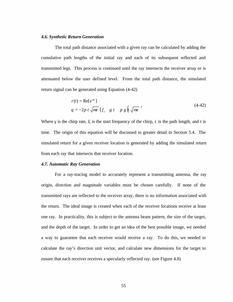
55
4.6. Synthetic Return Generation
The total path distance associated with a given ray can be calculated by adding the
cumulative path lengths of the initial ray and each of its subsequent reflected and
transmitted legs. This process is continued until the ray intersects the receiver array or is
attenuated below the user defined level. From the total path distance, the simulated
return signal can be generated using Equation (4-42)
( ) ( )22
]Re[)(
µετγπγµετπθ
θ
++−=
=
tf
etr
c
j
(4-42)
Where γ is the chirp rate, fc is the start frequency of the chirp, τ is the path length, and t is
time. The origin of this equation will be discussed in greater detail in Section 5.4. The
simulated return for a given receiver location is generated by adding the simulated return
from each ray that intersects that receiver location.
4.7. Automatic Ray Generation
For a ray-tracing model to accurately represent a transmitting antenna, the ray
origin, direction and magnitude variables must be chosen carefully. If none of the
transmitted rays are reflected to the receiver array, there is no information associated with
the return. The ideal image is created when each of the receiver locations receive at least
one ray. In practicality, this is subject to the antenna beam pattern, the size of the target,
and the depth of the target. In order to get an idea of the best possible image, we needed
a way to guarantee that each receiver would receive a ray. To do this, we needed to
calculate the ray’s direction unit vector, and calculate new dimensions for the target to
ensure that each receiver receives a specularly reflected ray. (see Figure 4.8)

56
Figure 4.8 Automatic Ray Generation Example
The available information is:
scoordinater Transmitte - ][tcoefficienequation planeTarget - D] C B[A
scoordinateReceiver - ][
TTT
RRR
ZYX
ZYX
The variables that must be solved for are:
factor scaling -k
scoordinateon Intersecti - ][ ppp ZYX
Applying Equation (4-1), the target facet plane equation to the unknown intersection
coordinates, we have
0=+++ DCZBYAX ppp (4-43)
Subtracting the intersection coordinates from the transmitter coordinates gives a direction
vector of the transmitter to intersection point ray. The reflected ray direction vector can
be calculated by subtracting the intersection coordinates from the receiver location. The
Law of Reflection states that the angle made by the incident and normal vector is the

57
same as the angle made by the reflected and normal vector. The dot product of the
incident and reflected rays and the normal vector will give the projection of the rays in
the normal vector direction. Because the incident and reflected rays are not normalized,
the dot products must be scaled by a factor, k.
[ ])()()()()()( pTpTpTpRpRpR ZZCYYBXXAkZZCYYBXXA −+−+−=−+−+−
(4-44)
Factoring Equation (4-44) and combining,
pTpTpTpRpRpR kCZkCZkBYkBYkAXkAXCZCZBYBYAXAX −+−+−=−+−+−
TTTRRRpppppp kCZkBYkAXCZBYAXCZkCZBYkBYAXkAX +++−−−=−+−+− )()()(
RRRTTTppp CZBYAXAXBYCZkkCZkBYkAX −−−++=−+−+− )()1()1()1(
])[][][][())(1( RRRTTTppp ZYXCBAZYXCBAkCZBYAXk ⋅−⋅=++− (4-45)
By substituting Equation (4-43),
])[][][][())(1( RRRTTT ZYXCBAZYXCBAkDk ⋅−⋅=−−
][][])[]([))(1( RRRTTT ZYXCBAZYXCBAkDk ⋅−=⋅−−−
][][])[]([ RRRTTT ZYXCBAZYXCBAkkDD ⋅−=⋅−−
][][])[][( RRRTTT ZYXCBADZYXCBADk ⋅−−=⋅−−
][][][][
TTT
RRR
ZYXCBADZYXCBAD
k⋅+⋅+
= (4-46)
By substituting NINIR )(2 ⋅−=
)()]()()([2)( pRTpTpTpTp XXkAZZCYYBXXAXX −=−+−+−−−
)()]()()([2)( pRTpTpTpTp YYkBZZCYYBXXAYY −=−+−+−−−

58
)()]()()([2)( pRTpTpTpTp ZZkCZZCYYBXXAZZ −=−+−+−−− (4-47)
Xp, Yp, and Zp are then solved for using the Matlab polynomial solver. These values are
calculated for each receiver location.
This section described the ray-tracing procedure used in the simulation. This
specific implementation was designed to generate a simulated received signal to be used
with the ground penetrating radar system developed by Rome Labs. The GPR system
interprets this signal and uses it to generate an image of the scene. In the following
section, the Rome Labs system will be described in detail and the image formation
technique will be discussed.

59
5. Description of System
The simulator described in this thesis was designed to be used with a GPR image
formation processor developed by Rome Labs, which will be described in this chapter.
The Rome Labs system combines the principles of synthetic aperture and ground
penetrating radar and was designed for deep soil penetration. The system uses a bow-tie
transmit antenna to transmit a linearly chirped signal into an underground medium. The
returns are measured at several locations within a receiver array grid using another bow-
tie antenna. By aligning the returns measured at each receiver location in range and
adding them coherently, an image of the underground scene can be generated. (See
Figure 5.1)
Figure 5.1 Rome Labs GPR Configuration
5.1. Transmission and Reception
Figure 5.2 is a block diagram representation of the Rome labs transmitter and
receiver system.
X
Y
Z
Transmitter
Receiver Array

60
Figure 5.2 Rome Labs Transmitter and Receiver System
The Rome labs system uses a linear frequency modulated continuous wave waveform.
This allows for accurate timing and control, while providing low peak power and high
dynamic range. [22] The signal is down-ramp linear frequency modulated from 66 to 6
MHz over 2 milliseconds. The frequency range was selected to achieve the desired 3 ft
resolution and avoid attenuation associated with the 160 ft maximum depth of ground
penetration. [22] The pulse is triggered by a first in, first out (FIFO) trigger through the
personal computer. The waveform is generated by an arbitrary waveform synthesizer and
amplified to 10 watts, as shown schematically in Figure 5.1. A linear weighting function
is applied at the waveform synthesizer to account for attenuation variations at different
frequencies and ensure a level transmitted signal.
The signal is transmitted by a 22 ft by 5 ft bow-tie antenna. The bow-tie antenna
was selected because it is wideband, directive, planar, efficient, and easily fabricated
Transmit Antenna Receive Antenna

61
[22]. The antennas are constructed of half-inch aluminum pipes and Plexiglas and rest
directly on the ground. A balun is added to the antenna and adjusted to match the
impedance of the feed cable. The receiver is a smaller bow-tie antenna, of dimensions 14
ft by 3 ft.
The received signal is demodulated by mixing it with a reference waveform that is
offset in frequency by 250 KHz. The reference and transmitted signals are both generated
by the arbitrary waveform synthesizer and triggered by the same FIFO trigger, ensuring
that the reference waveform and the transmitted waveform are coherent. The output of
the mixer is a signal containing a number of frequency components that are range
dependent. Each frequency component contained in the dechirped signal corresponds to
a return from a different scatterer in the scene. Mixing the received signal with a
frequency offset reference downconverts the signal to an intermediate frequency.
The analog dechirped signal is converted into a discrete signal using a 16-bit
analog to digital converter with a 1 MHz sample rate. The digital dechirped signal is then
interfaced into the personal computer.
To obtain data from the entire data grid, the receive antenna is moved to each
point in the receiver array grid. At each point, 2000 pulse samples are received and
averaged in the personal computer. The location of each receiver location relative to the
transmitter is measured and recorded using surveying equipment. After the averaged
return signal has been input into the computer, it is saved in a file that corresponds to
each receiver location. The relative position of each of the receiver locations is saved to
a file as well. This information is input into a GUI program developed by Rome labs to

62
perform the processing and generate an image of the scene. The GUI program can be
broken into two stages, the pre-processing stage, and the SAR processing stage.
5.2. Pre-Processing
After the input signal has been demodulated, each receiver location contains data
that is composed of distance dependant frequency components. Each of the frequency
components that comprise the demodulated signal correspond to a return from a different
scatterer in the scene. The objective of the pre-processing stage is to subject the
demodulated input data to several layers of signal processing to correct for undesired
effects. The block diagram of the pre-processing stage is shown as Figure 5.3.
Figure 5.3 Rome Labs Pre-Processing System
The first operation performed in the pre-processor is I and Q channel
demodulation. This step enables phase information to be taken from the received signal.
Two different I and Q demodulation techniques were used at different development
stages of the Rome Labs system. The first approach used separate channels to collect the
I and Q signals. The two different channels are sampled at the same frequency, 90
degrees out of phase of each other. The other approach involves using only one channel.

63
The input data signal is sampled at a rate four times above the 250KHz demodulation
frequency. Alternating data points of the sampled signal are then taken. A Hilbert
transform is performed on the signal, resulting in two signals, one corresponding to the I
channel and one to the Q channel, each containing half the number of samples of the
original signal.
The next step in the pre-processing stage is dispersion correction. The transmit
signal used in this system is linear frequency modulated from 66 to 6 Mhz. Within this
frequency range, the velocity of the transmitted signal through the medium is subject to
dispersion. The dispersion correction algorithm adds a phase component to the received
signal to compensate for the variation introduced by dispersion. The dispersion phase
correction is calculated as a function of chirp frequency and applied to each receiver
location. If dispersion is not adequately corrected for, the demodulated signal will retain
some frequency variation after it has been dechirped.
After the dispersion correction has been performed, the signal is high pass filtered
to remove direct path signal components. The transmit and receive antenna have a multi-
directional gain pattern and therefore are not directed solely into the ground. It is possible
for the receiver to receive a pulse from the transmitter that has traveled directly through
the air from the transmitter, without propagating through the ground. This is known as
direct path. Electromagnetic waves travel about four times faster through the air than
through the ground. Even if the difference in path distances between the direct path and a
valid path through the ground is similar, the direct path return will be received before
even the closest return from a valid ground path. After demodulation, the signal is

64
composed of many frequency components. The frequency of the signal components
varies directly with time delay. The time delay associated with a direct path signal is
significantly shorter than the time delay associated with a valid path. The frequency
components of the direct path signals are therefore much lower than the valid signal
returns. The frequency components of the signal caused by direct path can be removed
by means of a high pass filter.
After the signal has been filtered to remove the direct path signal component, the
magnitude of the signal is normalized to correct for attenuation. Attenuation is frequency
dependent, and therefore the higher frequency components of the chirped signal are more
affected by attenuation than the lower frequencies. The objective of the attenuation
correction is to correct the entire received signal to the same level, so the attenuation
correction must be frequency dependant. To calculate the normalization filter, the
magnitude of the attenuated signal is fit to a fifth order polynomial envelope function
across the entire received signal. The envelope function is calculated at each of the
receiver locations and then averaged. If a specific frequency range within the received
signal is consistently heavily attenuated, it will be reflected in the averaged envelope.
The incoming signal is then multiplied by the inverse of the averaged amplitude function.
If the envelope function is heavily attenuated over a certain frequency range, it will have
a lower magnitude in that range. By multiplying the input signal by the inverse of the
envelope function, heavily attenuated portions of the signal will be boosted more than
other portions with less attenuation.

65
To explain the Autoregressive Estimate and Hanning window blocks of the
preprocessing diagram, it is useful to review some signal processing concepts. When a
sinusoidal function is multiplied by a rect function in the time domain, it creates a sinc
function in the frequency domain. The smaller the rect function is, the higher the
sidelobes of the sinc function. A similar effect is occurring with the demodulated signal.
The sinusoidal signal of the demodulated signal is observed within a time window, which
has the same effect on the frequency components of the signal as a rect function. A
Hanning window is a signal processing technique that is frequently used to decrease the
sidelobes of the sinc function caused by multiplication of a sinusoidal signal by a rect
function. A Hanning window function is demonstrated in Figure 5.4(a-c).
Figure 5.4a A Time Windowed Sinusoid

66
Figure 5.4b Hanning Filter
Figure 5.4c Hanning Filter Applied to Windowed Signal
While the Hanning function improves the sidelobes of a function, it also removes some of
the information from the beginning and end of the signal, as can be seen in Figure 5.4c.
In order to insure that all of the input data is included in the Hanning window,
interpolated data is added to the beginning and end of the actual data.
5.3. SAR Processing
After the data has been conditioned and unfavorable effects have been removed, it
is sent to the SAR processor. The SAR processor separates the frequency components

67
received at each receiver location and sorts them according to which region of the scene
they were reflected from. It then generates an image based upon the location and
magnitude of the return.
The SAR processing procedure is described in Figure 5.5.
Figure 5.5 Rome Labs SAR Processing System
Before SAR processing takes place, the scene of interest, or user volume must be divided
into voxels, or three dimensional volume pixels. The user specifies the size of the voxels
used in the GUI. The first step of the SAR processing stage, in the bottom left corner of
Figure 5.5, is to select a voxel from the user volume. This voxel is referred to as the
voxel under test (VUT). We will call the first VUT selected in the scene VUT 1. An
initial receiver location within the receiver array is also selected, as pictured in the upper
left portion of Figure 5.5. We will call this receiver location Receiver 1. The Euclidean
1
2
5
3 4
6
7

68
distance from the transmitter to VUT1 to Receiver 1 is first calculated. This distance will
be referred to as the reference path distance, ∆(x,y,p). If the scene is to be referenced to a
point other than the transmitter, a correction can be added to the reference path distance.
The next step in SAR processing, depicted in the upper right portion of Figure 5.5
is to calculate the reference phase associated with the reference path distance. This is
done by first calculating the wavelength of the frequency and then using Equation (5-1).
( ) 22 τγπγτπϕ ⋅⋅++⋅⋅−= tfcr (5-1)
Where ϕr is the reference phase, τ is the time delay associated with the reference path
distance, fc is the frequency offset, and γ is the chirp rate. Equation (5-2) is then used to
shift the input data, gm,n(x,y,t) by the reference phase.
),,,(,,
,),,(),,,(' ptyxjnmnm
nmetyxgptyxg ϕ−⋅= (5-2)
If the signal at Receiver 1 contains a signal component from VUT 1, the exponential
function from Equation (5-2) will cancel with the time-varying portion of gm,n(x,y,t) and
there will be a large DC component of g’m,n(x,y,t,p). The samples of the received signal
are then summed, returning the DC value of the return.
After Equation (5-2) has been performed for VUT 1 and Receiver 1, the next
receiver location is selected, Receiver 2. A new reference path distance is calculated
from the transmitter to VUT 1 to Receiver 2. The new reference phase is calculated
using Equation (5-1) and g’m,n(x,y,t,p) is calculated using Equation (5-2). The new DC
value for g’m,n(x,y,t,p) at Receiver 2 is added to the DC value calculated at Receiver 1.
This process is continued for every receiver in the receiver array. After the last receiver

69
location has been calculated, the next VUT value (VUT 2) is selected and the process is
started again.
After a value has been obtained for every voxel in the scene, an image is
generated by assigning these values to a three-dimensional image representation of the
scene. Each VUT corresponds to a certain voxel in the image representation, and the
VUT value is assigned to that voxel.
5.4 GPR Simulation
To test the operation of the GPR software, Rome Labs developed a simulation
program that generates an ideal, analytical return from a perfectly diffuse point reflector
target. Perfectly diffuse point reflectors are reflectors of infinitesimal size that reflect a
transmitted signal equally in every direction. A target is generated by combining a
number of perfectly diffuse reflectors in a scene to approximate the target shape. Each of
these perfectly diffuse reflectors reflect an equal magnitude signal to each of the receivers
in the receiver array.
To create the simulation, the transmitted and received signal must be simulated
mathematically. The transmitted signal generated by the Rome labs GPR system is a
linear frequency modulated, sinusoidal signal. It can be expressed analytically using
Equation (5-3).
)2cos()( 20 ttfAts c γππ += (5-3)
In this equation, s(t) represents the transmitted signal, A0 represents the maximum
amplitude of the signal, fc is the starting frequency, t is time in seconds, and γ is the chirp

70
rate. Equation (5-3) is similar to a sinusoidally varying signal, except that the second
term in the cosine function increases the frequency as a function of time squared.
Assuming a loss-less environment, when the transmitted signal described by
Equation (5-3) is applied to a scene, the signal measured at the receiver will be equal to
the transmitted signal delayed in time. The length of the delay is determined by the
propagation time from the transmitter to the reflector, and then to the receive antenna.
This delay time is a factor of the distance traveled by the signal and the dielectric
properties of the material. If the signal takes τ seconds to travel from transmitter to
receiver, the received signal for a given scatterer can be expressed by Equation (5-2).
( ) ( )22cos()()( τγπτπ −+−= ttftatR c (5-4)
Where R(t) is the received signal as a function of time. The amplitude a(t) is expressed
as a function of time because the signal will experience greater attenuation as it travels
through a lossy medium. Because this attenuation is a function of distance or range, it is
also a function of time.
After the signal is received, it is demodulated. Demodulation involves removing
the original transmitted signal from the received signal. This is done by downconverting
the received signal. Downconversion is done by first multiplying the received signal,
which has been delayed in time, by the transmitted signal and then performing lowpass
filtering. The signal used to downconvert the received waveform is scaled in frequency
by an intermediate frequency, fif. Equations (5-5) through (5-9) show the
downconversion of the received signal. For convenience, the following substitutions can
be made for the transmit and received signals:

71
( ) ( )2
2
2
)2(
τγπτπβ
γππα
−+−=
−=
ttf
ttf
c
c (5-5)
[ ])cos()cos(21
)cos()cos()()(
βαβα
βα
++−=
=⋅ tRts (5-6)
The higher frequency component of this function is removed in the low pass filtering
leaving
)cos(21
)( βα −=tr (5-7)
Equation (5-7) can be simplified by substituting θ for (α-β), leaving
)Re(21
)cos(21
)( θθ jetr == (5-8)
where
(5-9)
Equation (5-7) can be broken down into three different terms:
( )
TermFrequency IF 2Term Phase Video Residual
TermsFrequency Range andDoppler 22
tf
tf
if
c
⋅⋅⋅
⋅+⋅−
πτγπ
γτπ
The intermediate frequency term can be removed by downconverting the signal
by the intermediate frequency term and then low pass filtering. Removal of the IF term
yields:
( ) 22 τγπγτπθ ++−= tf c (5-10)
( ) tftf ifc πτγπγτπβαθ 22)( 2 +++−=−=

72
Up to this point, it has been assumed that the signal measured at the receiver is the
result of a signal that was only reflected by a single scatterer. The actual system will
receive a signal at each receiver location that contains returns from many different
scatterers. The uniform point source simulated returns at a single receiver location
contain a return from each of the perfectly diffuse scatterers that make up the simulated
target. For each scatterer, there will be a different delay, τ. The effect of the individual
delays from each scatterer can be calculated using Equation (5-10). The received signal
for a given receiver location can be calculated by summing the returns from each of the
individual scatterers. For a given receiver, m and N scatterers, the received signal can be
expressed as:
(5-11)
Where n = {1…N} references each individual scatterer.
Equation (5-11) is a mathematical representation of a return signal received at one
of the receiver locations. The simulated signal contains all of the individual returns from
each of the scatterers in the scene. It can be subjected to the same SAR processing as an
actual received signal to extract the contribution of each scatterer in the scene.
This section described the processing involved in generating a scene using the
Rome Labs System. The simulated returns generated using the ray-tracing simulation
can be input into the GPR processing system to generate a simulated scene image. In the
following section, several images are generated using ray-tracing simulated returns and
the Rome Labs GPR system.
]Re[)( ,
1 ,
nmjN
n nmeta θ⋅∑
=

73
6. Results
To assess the performance of the ray-tracing simulator, several scene
configurations were created and run through the Rome Labs GPR processing software.
The scenes were selected to reflect different target, transmitter, and receiver array
locations and orientations. The size of the target, the size of the receiver array, and the
number of receivers in the receiver array were also varied. The transmitted ray direction
were either selected manually or using the automatic ray generator.
This section contains images showing the results of the data set runs. Two images
were generated for each data set: the scene configuration image and the GPR processed
image. The scene configuration images depict the transmitter, the faceted target, and the
receiver array. The transmitter is represented by a bow-tie shaped frame. The faceted
target appears as a three-dimensional box with the facets visible on the outside. The
receiver array is represented by a two-dimensional light blue rectangle. The rays are
represented by dark blue lines extending from the transmitter. For clarity, only rays that
propagate to a valid target are pictured, although additional rays may have been generated
in the simulation. The GPR processed image shows the image generated by the Rome
Labs GPR processing software. A reference target image has been superimposed upon
the GPR processed image to show the location and proportions of the actual target.
Throughout this section, the dimensions and positions of the transmitter, target,
and receiver arrays are specified in feet. They are expressed in Cartesian coordinates, as
(X dimensions, Y dimensions, Z dimensions) or (X location, Y location, Z location). The

74
relative dielectric permittivity of the target was set to 2 and the relative dielectric
permittivity of the surrounding scene was set to 15.
The Rome Labs system assigns a threshold to the voxels magnitude values in the
scene. The generated image is composed of each voxel in the scene that exceeds this
magnitude threshold. For the images in this section, the threshold was set to the top third
of the magnitude values of the voxels in the scene.
6.1 Automatic Ray Generation
The automatic ray generator was used to generate the rays used in data sets 1-7.
The automatic ray generator creates the ray equations such that a ray is received at every
receiver location, after being specularly reflected from the target. The target’s size and
location in the X and Y dimensions are also adjusted to ensure that each receiver in the
array receives a ray. The size and location of the target in the Z dimension are as
specified by the user. Automatic ray generation is a useful tool to observe certain
characteristics of scene configurations, ensuring that a sufficient number of rays are
received by the receiver array.

75
Data set 1:
Transmitter Origin:(0,50,0)
Ray Generation:Automatic
Receiver ArrayLocation:
(100,50,0)
Receiver ArrayDimensions:
(100,100,0)Receiver Spacing X:
10Receiver Spacing Y:
10Target Location:
(52.5, 52.5, -40)Target Size:
(52, 52, 20)Table 6.1: Data Set 1 Scene Configuration Information
Figure 6.1a. Data Set 1 Scene Configuration Image
The images generated with the scene orientation used in data set 1 are intended to
be a means of comparison of effects observable using the automatic ray generator. The
orientation of the projected rays can be observed in Figure 6.1a. Due to the use of the

76
automatic ray generator, the top of the target has a large number of reflections directly to
the receiver array. There are not any rays that transmit through the target.
The image generated by the Rome Labs GPR processing software for data set 1 is
depicted in Figure 6.2b. The processed image is fairly consistent with the superimposed
original target for about one half of the length of the target. Behind the target, there is a
tail that extends from the top of the target towards the transmitter.
Figure 6.1b. Data Set 1 GPR Processed Image
6.1.1 Transmitter Orientation
Data sets 2 and 3 were set up similarly to data set 1, except the position of the
transmitter was varied in the Y dimension. These data sets were performed to observe

77
the effects of varying the position of the transmitter laterally compared to the receiver
array.
Data set 2:
Transmitter Origin:(0,0,0)
Ray Generation:Automatic
Receiver ArrayLocation:
(100,50,0)
Receiver ArrayDimensions:
(100,100,0)Receiver Spacing X:
10Receiver Spacing Y:
10Target Location:
(52.5,27.5,-40)Target Size:
(52, 52, 20)Table 6.2: Data Set 2 Scene Configuration Information
Figure 6.2a. Data Set 2 Scene Configuration Image

78
The scene configuration and GPR processed images for data set 2 are depicted in
Figure 6.2(a-b). The configuration for this scene is the same as that for data set 1, except
that the transmitter has been shifted to the X, Y, and Z coordinates (0,0,0). The target
dimensions are (52, 52, 20) and the target is centered at (52.5, 27.5, -40). There are no
rays that are transmitted into the target.
The processed image is similar to the image in data set 1. There is a tail present
in the image that extends towards the transmitter, but the transmitter is located at the
origin, so the tail extends at an angle.
Figure 6.2b. Data Set 2 GPR Processed Image

79
Data set 3:
Transmitter Origin:(0,100,0)
Ray Generation:Automatic
Receiver ArrayLocation:
(100,50,0)
Receiver ArrayDimensions:
(100,100,0)Receiver Spacing X:
10Receiver Spacing Y:
10Target Location:
(52.5, 77.5, -40)Target Size:
(52, 52, 20)Table 6.3: Data Set 3 Scene Configuration Information
Figure 6.3a. Data Set 3 Scene Configuration Image
In data set 3, depicted in Figure 6.3(a-b), the transmitter is moved along the Y
axis to the edge of the receiver array at (0, 100, 0). The resulting target is positioned at

80
(52.5, 77.5, –40) and has dimensions of (52, 52, 20). Like sets 1 and 2, there are no rays
that transmit into the target.
Similar results were obtained in the GPR processed image as in data set 2. There
is a tail that extends from the top of the superimposed target towards the transmitter,
which is closer to the viewer as the image appears in Figure 6.3b.
Figure 6.3b. Data Set 3 GPR Processed Image
6.1.2 Receiver Orientation
In data sets 4-7, the size of the receiver array and the spacing between the
receivers was varied. The number of receivers in the array was calculated based upon the
size of the receiver array. Therefore, larger receiver arrays had a greater number of
receivers within them. The spacing between the receivers was also varied, making the
array either more or less densely populated with receivers.

81
Data set 4:
Transmitter Origin:(0,50,0)
Ray Generation:Automatic
Receiver ArrayLocation:
(100,50,0)
Receiver ArrayDimensions:
(100,100,0)Receiver Spacing X:
5Receiver Spacing Y:
5Target Location:
(51.25,51.25,-40)Target Size:
(52, 52, 20)Table 6.4: Data Set 4 Scene Configuration Information
Figure 6.4a. Data Set 4 Scene Configuration Image
The fourth data set was generated using a receiver array with a denser
concentration of receivers. The receivers in the array were spaced at 5 ft intervals in both
the X and Y dimensions. The target’s X and Y dimensions, generated by the automatic

82
ray generator, were found to be (52, 52, 20) and were centered at (51.25, 51.25, -40).
There are considerably more rays reflected from the top of the target, but there are no
rays that are transmitted into the target.
Figure 6.4b shows the GPR processed image generated using data set 4. There is
a very strong return reflected from the top of the target. As in previous data sets, there is
a tail extending from the target top towards the transmitter.
Figure 6.4b. Data Set 4 GPR Processed Image

83
Data Set 5:
Transmitter Origin:(0,50,0)
Ray Generation:Automatic
Receiver ArrayLocation:
(100,50,0)
Receiver ArrayDimensions:
(100,100,0)Receiver Spacing X:
20Receiver Spacing Y:
20Target Location:
(51.25,51.25,-40)Target Size:
(52, 52, 20)Table 6.5: Data Set 5 Scene Configuration Information
Figure 6.5a. Data Set 5 Scene Configuration Image
In data set 5, the simulation was run with a less densely populated receiver array,
with the receivers spaced at 20 ft intervals in the X and Y dimensions. The GPR
processed image for data set 5 is shown as Figure 6.5b. The image is clustered towards
the front of the superimposed target. Only a small percent of the generated image is

84
actually in the immediate area of the target. There is a pronounced tail extending towards
the transmitter.
Figure 6.5b. Data Set 5 GPR Processed Image

85
Data Set 6:
Transmitter Origin:(0,75,0)
Ray Generation:Automatic
Receiver ArrayLocation:
(100,75,0)
Receiver ArrayDimensions:
(100,150,0)Receiver Spacing X:
10Receiver Spacing Y:
10Target Location:
(52.5,77.5,-40)Target Size:
(52,77,20)Table 6.6: Data Set 6 Scene Configuration Information
Figure 6.6a. Data Set 6 Scene Configuration Image
In data set 6, the receiver array was expanded to 100 ft in the X direction and 150
ft in the Y direction. The receiver array is centered at (100, 75, 0). Because the receiver
array size was expanded and the spacing of the receivers was held constant, the number

86
of receivers increased from 121 to 176. The transmitter was moved to (0, 75, 0) so that it
would remain centered between the sides of the receiver array in the Y dimension.
Figures 6.6(a-b) shows the scene configuration of data set 6. The GPR processed
image for data set 6 is shown as Figure 6.6b. The image generated covers almost the
entire target in the Y direction, but less than half of the target in the X direction. A tail
extends from the top of the target towards the transmitter in the X direction.
Figure 6.6b. Data Set 6 GPR Processed Image

87
Data Set 7:
Transmitter Origin:(0,50,0)
Ray Generation:Automatic
Receiver ArrayLocation:
(100,50,0)
Receiver ArrayDimensions:
(150,100,0)Receiver Spacing X:
10Receiver Spacing Y:
10Target Location:
(52.5,52.5,-40)Target Size:
(77,52,20)Table 6.7: Data Set 7 Scene Configuration Information
Figure 6.7a. Data Set 7 Scene Configuration Image
In data set 7, the size of the receiver array was increased in the X direction. The
receiver array was of size (150, 100, 0) with receivers spaced every 10 ft in the Y
direction and every 10ft in the X direction. As can be seen in Figure 6.7a, several rays
reflected repeatedly from the top of the target and off of the bottom of the ground;
however, no rays were transmitted into the target.

88
The GPR processed image for data set 7 is shown as Figure 6.7b. The image
extends approximately halfway across the target. There is a tail that extends from the top
of the target towards the transmitter.
Figure 6.7b. Data Set 7 GPR Processed Image
6.2 Manually Generated Rays
In data sets 8-13, the size and position of the target was varied. In all of the data
sets in this section, the transmitter and receiver array orientation was the same. The
receiver array was a (100, 100, 0) ft square with receivers spaced at 10ft intervals in the
X and Y directions. The receiver array was centered at (100, 50, 0). In this data set, the
transmitted rays were sent from a transmitter located at (0, 50, 0) and generated manually
without the aid of automatic ray generator. It is recommended in the Xpatch manual that

89
10 rays are projected at a target per each unit of wavelength. It also states that for an
uncomplicated target, 3 rays per unit of wavelength are sufficient [8]. Because our target
is not complicated, 3 rays per unit of wavelength were used.
To determine the number of rays to use, it was first necessary to calculate the
wavelength of the transmitted signal. The wavelength can be calculated from:
εµλ
fc
= (6-1)
Where f is the frequency of the transmitted signal, ε is the relative dielectric permittivity
and µ is the relative magnetic permeability. The relative dielectric permittivity assumed
in the simulation was 15. This is a typical dielectric constant for granite or soil [23]. The
magnetic permeability is frequently assumed to be 1 in GPR simulations [7]. The
transmitted frequency was 66-6 MHz. We will use the higher frequency, which requires
a greater number of rays, as a worst-case scenario. The wavelength is calculated to be
1.17 m, or 3.84 ft.
The following example will demonstrate how the number of rays is chosen. Take,
for example a target of dimensions (20, 40, 20) ft. The dimensions in units of wavelength
are (5.20, 10.41, 5.20)λ. The maximum area of this object seen by the transmitter in the
scene configuration defined above is seen when the target is tilted at a 45-degree angle.
The maximum area is:
222 55.7641.1020.520.5 λ=×+ (6-2)

90
It is recommended that 3 rays per linear unit of wavelength are sent. In a two
dimensional area, 9 rays must be transmitted per unit of λ2 . This equates to 689 rays.
The wavelength and antenna dimensions can be used to calculate if the system is
operating in the Fresnel or far field. The extent of the Fresnel field is from D2 /4λ to D2
/λ. The far field extends past D2 /λ. Using the wavelength value calculated above and an
antenna diameter of 22 ft, we find that the Fresnel field extends from 38.5 ft to 126.2 ft
away from the transmitter. The far field extends past 126.2 ft from the transmitter. The
target positions used in this section are within the Fresnel field. As discussed in Section
4, transmitters operating in the near field can be modeled using rays that originate at the
transmitter location and extend radially away from it. This technique will be used to
model the transmitted signal in this section.

91
Data Set 8:
TransmitterOrigin: (0,50,0)
Ray Generation:Manual
Receiver ArrayLocation:
(100,50,0)
Receiver ArrayDimensions:
(100,100,0)Receiver SpacingX: 10
Receiver SpacingY: 10
Target Location:(50,50,-40)
Target Size:(20,40,20)
Ray Array Size: X26
Ray Array Size: Y26
Table 6.8: Data Set 8 Scene Configuration Information
Figure 6.8a Data Set 8 Scene Configuration Image
Data set 8, and the images associated with it were intended to be useful in
comparison of different scene orientations used with manually generated rays. In data set
8, the target is of dimensions (20, 40, 20) and is centered at (50, 50, -40). The transmitter

92
projects a 26 by 26 array of rays towards the target. As can be seen in Figure 6.8a, many
rays contact the side of the target and are not transmitted into the target. This is because
the rays are incident at a glancing angle. Snell’s law states that rays are more likely to
penetrate a target at a more direct angle. The rays that extend to the receiver array are
specularly reflected from the top of the target.
The GPR processed image for data set 8 shows a thick image, which covers the
majority of the top of the target. There is also a dense tail that extends from the top of the
target in the X dimension towards the transmitter.
Figure 6.8b Data Set 8 GPR Processed Image
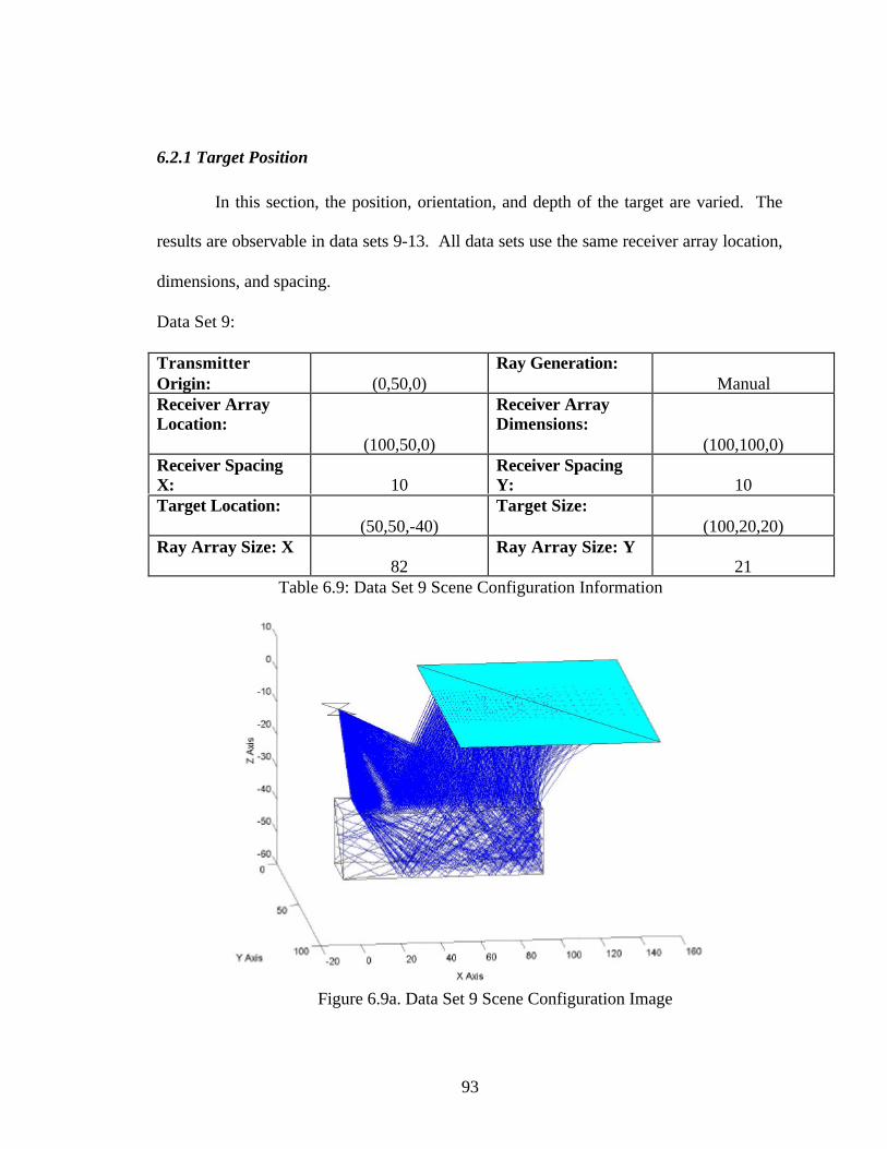
93
6.2.1 Target Position
In this section, the position, orientation, and depth of the target are varied. The
results are observable in data sets 9-13. All data sets use the same receiver array location,
dimensions, and spacing.
Data Set 9:
TransmitterOrigin: (0,50,0)
Ray Generation:Manual
Receiver ArrayLocation:
(100,50,0)
Receiver ArrayDimensions:
(100,100,0)Receiver SpacingX: 10
Receiver SpacingY: 10
Target Location:(50,50,-40)
Target Size:(100,20,20)
Ray Array Size: X82
Ray Array Size: Y21
Table 6.9: Data Set 9 Scene Configuration Information
Figure 6.9a. Data Set 9 Scene Configuration Image

94
In data set 9, the target is rectangular in shape with its longer dimension in the X
dimension. The target size is (100, 20, 20) and it is centered at (50, 50 ,-40). An 82 by
21 array of rays is transmitted at the target. A large number of rays are reflected from the
top of the target. There are also a large number that penetrate into the target. The
penetrating rays make several reflections within the target and many intersect the receiver
array. Some of the rays that are reflected from the top of the target are reflected towards
the receiver array, reflect from the bottom of the receiver array, and are reflected from the
target again towards the receiver array.
The GPR processed image of data set 9 shows a dense image located closest to
the transmitter in the X direction. There is a broken tail that extends from the top of the
target towards the transmitter in the X direction.
Figure 6.9b. Data Set 9 GPR Processed Image

95
Data Set 10:
TransmitterOrigin: (0,50,0)
Ray Generation:Manual
Receiver ArrayLocation:
(100,50,0)
Receiver ArrayDimensions:
(100,100,0)Receiver SpacingX: 10
Receiver SpacingY: 10
Target Location:(50,50,-40)
Target Size:(20,100,20)
Ray Array Size: X21
Ray Array Size: Y82
Table 6.10: Data Set 10 Scene Configuration Information
Figure 6.10a. Data Set 10 Scene Configuration Image
The same target dimensions used in data set 9 were used in data set 10, except the
orientation of the target is rotated so the longer dimension of the target is oriented in the
Y dimension. An array of 21 by 82 rays was transmitted at the target from the
transmitter. As in data set 8, many rays impact the side of the target and are not

96
transmitted into the target, making the only rays that extend to the receiver array those
that are reflected from the top of the target.
Figure 6.10b shows the GPR processed image of data set 10. The image
generated does not extend to the sides of the target, but is centered in the Y dimension.
There is a tail that extends from the top of the target towards the transmitter.
Figure 6.10b. Data Set 10 GPR Processed Image

97
Data Set 11:
TransmitterOrigin: (0,50,0)
Ray Generation:Manual
Receiver ArrayLocation:
(100,50,0)
Receiver ArrayDimensions:
(100,100,0)Receiver SpacingX: 10
Receiver SpacingY: 10
Target Location:(100,50,-40)
Target Size:(20,40,20)
Ray Array Size: X26
Ray Array Size: Y26
Table 6.11: Data Set 11 Scene Configuration Information
Figure 6.11a. Data Set 11 Scene Configuration Image
In data set 11, the target was moved to the location (100, 50, -40). Because the
target is positioned directly underneath the receiver, there are no rays reflected from the
top of the target. The distance separating the transmitter and receiver caused the rays that

98
are incident on the side of the target to be at a more direct angle, allowing them to
transmit into the target. These rays are subject to several reflections within the target,
and many are reflected towards the receiver array.
The GPR processed image for data set 11 shows a significant amount of clutter,
making it difficult to determine the exact location of the target. There is a hemispherical
shaped clutter pattern with its bottom at approximately the position of the target. There
are two distinct erroneous images immediately below the bottom of the hemisphere.
Figure 6.11b. Data Set 11 GPR Processed Image

99
Data Set 12:
TransmitterOrigin: (0,50,0)
Ray Generation:Manual
Receiver ArrayLocation:
(100,50,0)
Receiver ArrayDimensions:
(100,100,0)Receiver SpacingX: 10
Receiver SpacingY: 10
Target Location:(50,50,-100)
Target Size:(20,40,20)
Ray Array Size: X26
Ray Array Size: Y26
Table 6.12: Data Set 12 Scene Configuration Information
Figure 6.12a. Data Set 12 Scene Configuration Image
In data set 12, a (20, 40, 20) target was lowered in the Z direction to a location of
(50, 50, -100). Similar to data set 8, few of the rays were transmitted into the target.
The only rays that intersect with the receiver array are those reflected from the top of the
target.

100
The resulting GPR processed image is approximately the same dimensions as the
target. The image has a less pronounced tail extending towards the transmitter and a
slight overhang extending in the positive X direction.
Figure 6.12b. Data Set 12 GPR Processed Image

101
Data Set 13:
TransmitterOrigin: (0,50,0)
Ray Generation:Automatic
Receiver ArrayLocation:
(100,50,0)
Receiver ArrayDimensions:
(100,100,0)
Receiver SpacingX: 10
Receiver SpacingY: 10
Target Location:(52,52,-100)
Target Size:(52,52,20)
Table 6.13: Data Set 13 Scene Configuration Information
Figure 6.13a. Data Set 13 Scene Configuration Image
Data set 13 was set up similarly to data set 12, except automatic ray generator was
used to generate the rays and size the transmitter to ensure a specular reflection to all of
the receiver locations. The size and location of the target are almost identical to those for

102
data set 1, except the target in data set 13 is at a depth of –100ft. The orientation of this
target caused some of the rays to be transmitted into the target.
The GPR processed image generated by data set 13 is shown in Figure 6.13b.
The image is focused towards the front of the target. The tail that is apparent on many of
the other images is gone in this image.
Figure 6.13b. Data Set 13 GPR Processed Image
6.2.2 Resolution / Number of Rays
The resolution of the image was varied in data sets 14-17. Two methods were
used to change the resolution. The first method was to alter the number of rays
transmitted into the scene. The second method was to change the voxel size used to
generate the image in the GPR processing GUI. The scene used for these runs had the

103
transmitter located at (0, 50, 0). The target was located at (50, 50, -40) and its size was
(20, 40, 20). The receiver array was centered at (100, 50, 0) with a size of 100ft by 100
ft. The receivers in the array were spaced at 10 ft in the X direction and 10 ft in the Y
direction.
Data Set 14:
TransmitterOrigin: (0,50,0)
Ray Generation:Manual
Receiver ArrayLocation:
(100,50,0)
Receiver ArrayDimensions:
(100,100,0)Receiver SpacingX: 10
Receiver SpacingY: 10
Target Location:(50,50,-40)
Target Size:(20,40,20)
Ray Array Size: X26
Ray Array Size: Y26
Table 6.14: Data Set 14 Scene Configuration Information
Figure 6.14a. Data Set 14 Scene Configuration Image

104
In data set 14, the voxel size setting in the GPR processing GUI was changed from 5 ft to
10 ft. This caused the GPR processed image to be larger and less defined than data set 8,
where the voxel size was set to 5 ft. The GPR generated image has a broken tail that
extends towards the transmitter, similar to the effects seen in data set 8.
Figure 6.14b. Data Set 14 GPR Processed Image
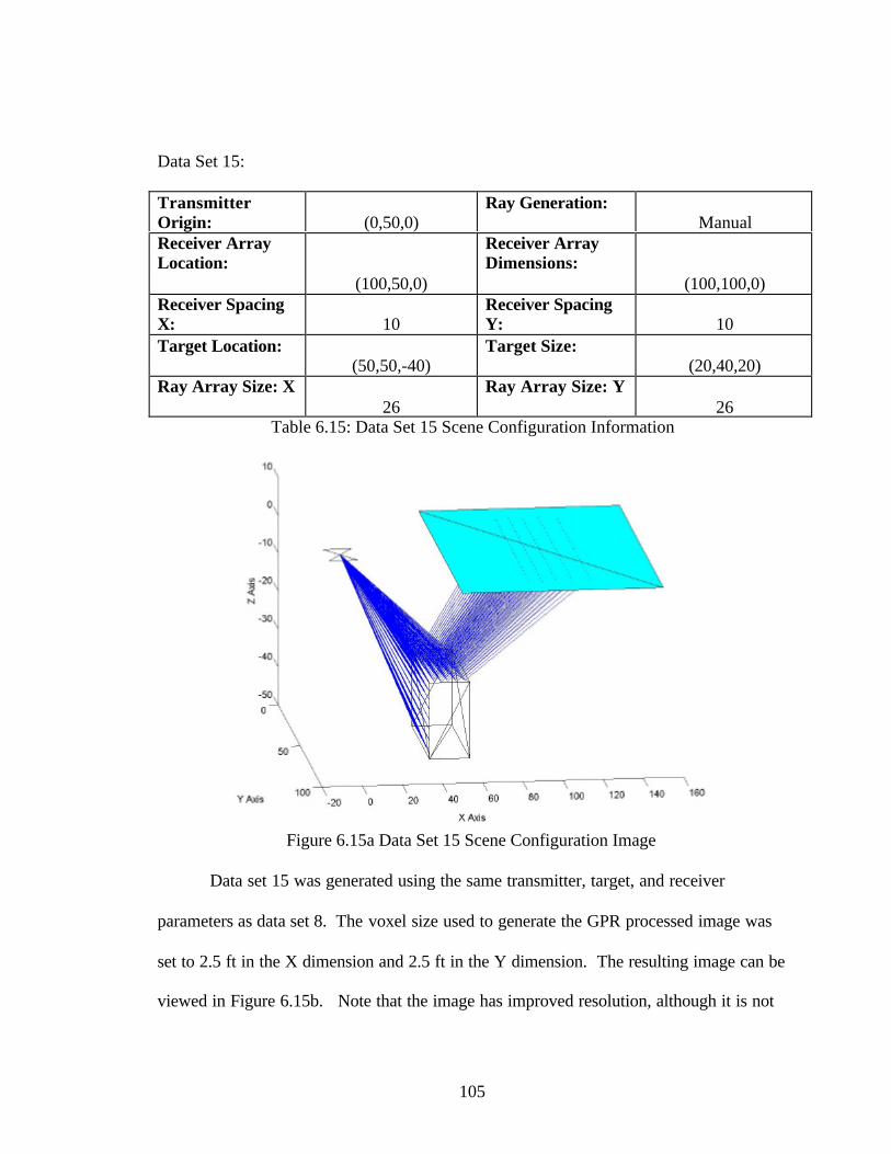
105
Data Set 15:
TransmitterOrigin: (0,50,0)
Ray Generation:Manual
Receiver ArrayLocation:
(100,50,0)
Receiver ArrayDimensions:
(100,100,0)Receiver SpacingX: 10
Receiver SpacingY: 10
Target Location:(50,50,-40)
Target Size:(20,40,20)
Ray Array Size: X26
Ray Array Size: Y26
Table 6.15: Data Set 15 Scene Configuration Information
Figure 6.15a Data Set 15 Scene Configuration Image
Data set 15 was generated using the same transmitter, target, and receiver
parameters as data set 8. The voxel size used to generate the GPR processed image was
set to 2.5 ft in the X dimension and 2.5 ft in the Y dimension. The resulting image can be
viewed in Figure 6.15b. Note that the image has improved resolution, although it is not

106
extremely different in shape than the image generated using data set 8.
Figure 6.15b. Data Set 15 GPR Processed Image

107
Data Set 16:
TransmitterOrigin: (0,50,0)
Ray Generation:Manual
Receiver ArrayLocation:
(100,50,0)
Receiver ArrayDimensions:
(100,100,0)Receiver SpacingX: 10
Receiver SpacingY: 10
Target Location:(50,50,-40)
Target Size:(20,40,20)
Ray Array Size: X52
Ray Array Size: Y52
Table 6.16: Data Set 16 Scene Configuration Information
Figure 6.16a. Data Set 16 Scene Configuration Image
Data set 16 was generated by using an array of 52 by 52 rays. Four times as many rays
were transmitted towards the target as compared to data set 8. The voxel size was reset to
5 ft. The resulting image, pictured in Figure 6.16b is very similar to the GPR processed
image generated using data set 8.

108
Figure 6.16b. Data Set 16 GPR Processed Image

109
Data Set 17:
TransmitterOrigin: (0,50,0)
Ray Generation:Manual
Receiver ArrayLocation:
(100,50,0)
Receiver ArrayDimensions:
(100,100,0)Receiver SpacingX: 10
Receiver SpacingY: 10
Target Location:(50,50,-40)
Target Size:(20,40,20)
Ray Array Size: X13
Ray Array Size: Y13
Table 6.17: Data Set 17 Scene Configuration Information
Figure 6.17a Data Set 17 Scene Configuration Image
In data set 17, a 13 by 13 ray array was used to generate the image. This is a
quarter of the rays transmitted in data set 8. The image generated can be viewed as

110
Figure 6.17b. The image is slightly less resolved, with some clutter in the front and rear
portions of the image.
Figure 6.17b Data Set 17 GPR Processed Image
6.3 Uniform Point Scatterer Simulation
In data sets 18-20, the uniform point scatterer simulator created by Rome Labs
was used to generate simulated images. The target used for these data sets consisted of a
two dimensional array of uniform point scatterers in the X and Y dimensions. The array
of scatterers was centered at (50, 50, -40). The dimensions of the array were 20 ft in the
X direction and 40 ft in the Y direction. The receiver array used in data sets 18-20 was of
dimensions 100 ft in the X direction and 100 ft in the Y direction, centered at (100, 50,
0). The receivers were spaced at 10 ft by 10 ft intervals within the receiver array.

111
In data set 18, the uniform point scatterers were spaced by 4 ft in the X direction
and by 8 ft in the Y direction. The GPR processed image shown in Figure 6.18 shows the
output of this run. The Image generated has a tail extending towards the transmitter in
the X direction and a jagged edge on the front portion of the image.
Figure 6.18. Data Set 18 GPR Processed Image
The scatterers were spaced by 2ft in the X direction and 4 ft in the Y direction in
data set 19. The GPR processed image generated from this run can be viewed as Figure
6.19. While the image has a tail extending towards the transmitter, the image from the
scatterer array is smooth and well resolved.

112
Figure 6.19. Data Set 19 GPR Processed Image
The final data set, data set 20, was generated using the uniform point scatterer
simulation with the scatterers spaced by 10 ft in the X direction and 20 ft in the Y
direction. The GPR processed image is shown in Figure 6.20. This image is
discontinuous in the Y dimension, showing several shapes from each line of scatterers in
the X direction.

113
Figure 6.20. Data Set 20 GPR Processed Image

114
7. Discussion
The images generated using the ray-tracing simulator in Section 6 are dependent
not only upon the size of the target, but also upon the configuration of the scene. This
section will discuss the characteristics of these images and the effects scene configuration
has upon them.
The path distance of each ray that is reflected from the target and received at a
receiver location is indicative of the range from the transmitter to the receiver via the
target. There is directional ambiguity associated with this range, as many points within
the scene can be associated with this same range value. The points of equal range for a
given transmitter location and receiver location form a three dimensional ellipse. This
ellipse is pictured in two dimensions in Figure 7.1. For a horizontally oriented target, the
bottom edge of the ellipse is located at the intersection point of the ray with the target.
The width of the ellipse is dictated by the range.
Figure 7.1 GPR Processing Directional Ambiguity Ellipse
Transmitter Receiver
Target

115
The directional ambiguity associated with each received ray scribes a different
ellipse. When a number of rays intersect the target in close proximity and are reflected
towards the receiver array, these ellipses may overlap. By combining several ellipses, the
directional ambiguity is reduced. In SAR processing, a magnitude value is assigned to
each voxel in the ellipse based upon the voltage of the received signal. The processed
image is created by additively combining the magnitude values of each voxel in the
ellipses.
One characteristic of many of the GPR processed images is a tail extending from
the top of the target towards the transmitter. This anomaly is caused by the overlap of
several ellipses that are spaced along the top of the target and steadily increasing in width
and will be referred to as the tail effect. This phenomenon is pictorially illustrated in
Figure 7.2, which shows a two dimensional representation in the X dimension.
Figure 7.2 Two Dimensional Representation of GPR Processed Image in X Dimension

116
The ellipses pictured are equally spaced at 5 units, and steadily increasing in width in the
X direction by 5 units, from left to right. In an imaged scene, the width of the ellipses
increase because the path distances are steadily increasing for specular reflections at
receiver locations further from the transmitter. The near proximity and overlap of these
ellipses cause a high magnitude value for the voxels in the area where the tail is formed.
Many of the images in Section 6 are shifted towards the side of the target closest
to the transmitter. This is also a function of the increasing focus of the ellipses. In Figure
7.2, several of the ellipses on the left side of the plot overlap. In an image generated
using the GPR processor, the magnitude of the voxels in this region would be greater than
the non-overlapping, wider ellipses on the right side of the image. This is the reason that
the transmitter side of the GPR processed image frequently has a greater magnitude than
the receiver side, an effect that will be referred to as range distortion.
Figure 7.3 Two Dimensional Representation of GPR Processed Image in Y Dimension

117
Figure 7.3 shows a two dimensional representation of increasing ellipses in the Y
dimension. The shortest path distance is associated with the center path in a scene that is
symmetric in the Y dimension. The path distances increase with increased deviation
from the center. In Figure 7.3, the ellipses are evenly spaced and steadily increasing in
width as they deviate from the center. In an image generated by the GPR processor, the
wider ellipses on either end would contribute to the narrow ellipse in the center, making
the magnitude of the voxels relatively high in the center of the image. There is a sparse
concentration of ellipses on the edges of the image, which would result in voxels of a
lower magnitude in that region. This effect will be referred to as cross-range distortion.
7.1 Automatic Ray Generation
The images in Section 6.1 were created using the automatic ray generator. The
direction of the transmitted rays and the size and position of the target were calculated to
ensure that each receiver in the receiver array received a ray that was reflected specularly
from the top of the target. Generating the rays this way allows the receiver array
parameters and target depth to be changed while ensuring that a resolvable scene will
result. It also generates a system of rays that are evenly spaced along the top of the
target, which is a useful way to observe the tail effect, range distortion, and cross-range
distortion.
The scene configuration used in data set 1 was selected to provide a basis for
comparison with other data sets in this section. As can be seen in Figure 6.1b, the image
generated in this data set have the characteristic tail and weighting on the transmitter side
of the target associated with the tail effect and range distortion. Figures 7.4 a and b

118
illustrate these effects in the X and Y dimensions. They show a two-dimensional
representation, although the actual generated ellipses are three-dimensional. The X
dimension representation shows a cut taken down the center of the scene at the
transmitter location. The Y dimension shows a cut taken along the first line of rays that
intersect with the target. These plots were not created using the GPR processing
software, but were generated using information from actual simulations. The foci and
spacing of the ellipses were calculated from the path distances of rays projected in data
set 1.
Figure 7.4 X and Y Ellipse Representation of Data Set 1
The actual ellipses effect that creates the scene are three dimensional, and can be
visualized by additively combining Figures 7.4 a and b. Figures 7.4a shows a high
density of ellipses in the X dimension along the top of the target and along the tail
extending in the direction of the transmitter. Figure 7.4b shows the ellipse diagram in the
Y dimension for data set 1. The ellipses are most concentrated at in the center of the
scene, a direct effect of cross-range distortion. This is consistent with the GPR processed
image of data set 1, Figure 6.1b.

119
7.1.1 Transmitter Orientation
The images created in Section 6.1.1 were generated by varying the position of the
transmitter relative to a fixed target and receiver location. The GPR processed images for
data sets 1,2, and 3 exhibit tail effect, range distortion, and cross-range distortion as a
result of the widening of the directional ambiguity ellipses. The shape of the generated
image is similar in each of the data sets, but the orientation is different. The tails
generated extend in the direction of the transmitting antenna. The generated images do
not extend to the side of the target opposite the transmitter.
7.1.2 Receiver Orientation
In data set 4, the density of receivers in the array was increased by a factor of four
over data set 1. Because the automatic ray generator was used, a greater concentration of
rays were reflected from the target and received at the receiver array. The ellipses
associated with these rays were spaced closer together than in data set 1. Figures 7.5 a
and b show the effect of decreasing the distance between ellipses.
Figure 7.5 X and Y Ellipse Representation of Data Set 4

120
Figure 7.5a is similar to Figure 7.4a, except the greater concentration of ellipses
extends along the target further in the X direction. The ellipses are also distributed over a
larger spacing in the Y dimension, resulting in less pronounced range and cross-range
distortion. Both of these features can be observed in Figure 6.4b, as the resolved image is
slightly larger compared to Figure 6.1b. The increased number of receivers in the array
created an image that was well resolved, following the contours of the target better than
the image generated using data set 1.
Figure 7.6 X and Y Ellipse Representation of Data Set 5
In data set 5, the decreased number of receivers within the receiver array has the
opposite effect. By using the automatic ray generator, one fourth of the rays used in data
set 1 were included in the scene. The ellipses generated in the image are spaced further
apart due to the spacing of the rays, as can be seen in Figure 7.6 a and b. By using the
automatic ray generator, one fourth of the rays used in data set 1 were included in the
scene. The ellipses generated in the image are spaced further apart due to the spacing of
the rays, as can be seen in Figure 7.6 a and b.

121
The GPR processed image, shown in Figure 6.5b has a less concentrated tail than
Figure 6.1b or 6.4b. The cumulative returns in the vicinity of the top of the target are
small compared to the relative magnitude along the tail of the image. The image is
concentrated in the Y dimension on the side of the target closest to the origin. This is
because there are more rays reflected towards the receiver array on that side of the target.
The size of the receiver array was varied in data sets 6 and 7. In data set 6, the
size of the receiver array was increased by 50 ft in the Y dimension. This added 55
additional receivers to the array, and consequently 55 additional rays to generate the
image. The GPR processed image generated can be viewed as Figure 6.6b. The image
created is wider in the Y dimension than the image created using the 100 ft by 100 ft
receiver array. The ellipse diagram for data set 6 is shown as Figure 7.7. The X
dimension cut is similar to that for data set 1 (shown as Figure 7.4a). The Y dimension
plot is similar to 7.5b, which was generated using a higher concentration of rays. The
Figure 7.7 X and Y Ellipse Representation of Data Set 6

122
increased receiver array size caused a greater number of ellipses in the Y dimension,
along with a greater spreading of the width of the ellipses.
In data set 7, the receiver array was extended in the X dimension. The GPR
processed image for this data set extends somewhat further in the X dimension than the
image generated in data set 1, although it is approximately the same size in the Y
dimension. Increasing the size of the receiver array caused a greater number of ellipses
in the X dimension with an increased range of ellipse widening. This effect is shown in
Figure 7.8.
Figure 7.8 X and Y Ellipse Representation of Data Set 7
7.2 Manual Ray Generation
Data sets 8-17 were formed using manual ray generation, which is required if a
specific antenna model is desired. The rays created by the manual ray generator are
evenly spaced in polar coordinates and aimed by the user. The rays therefore do not

123
intersect the top of the target at even Cartesian intervals, making it difficult to quantify
the tail effect, range distortion, and cross-range distortion, although these phenomena are
present. This section is used to demonstrate the image implications of different ray
parameters in the scene.
Data set 8 was used to provide a comparison benchmark for the other data sets in
the section. The image generated using data set 8 is included in Section 6 as Figure 6.8b.
Similar to the images in the previous section, data set 8’s image exhibits the tail effect.
The ray spacing when using manual ray generation is much smaller than when the
automatic ray generator is used, causing the generated image to cover the entire width of
the target in the Y dimension. The rays in the manual ray tracing runs are spaced at 3
rays per unit wavelength, while the automatically generated rays only include one ray per
receiver in the receiver array.
7.2.1 Target Position
The scene imaged in data set 9 includes a target that is stretched to cover the
entire scene of interest and rotated so the long dimension is in the X direction. There are
a large number of transmitted rays within the target, many of which eventually intersect
with the receiver array. There are also several rays that reflect repeatedly between the top
of the target and the ground / air interface, ultimately intersecting the receiver array.
These rays can cause some anomalies, as their path distance may be much longer than the
direct path distance to the target. The GPR processed image, shown in Figure 6.9b,
shows some anomalies in the upper left side of the image, however the anomalies are not
as extensive as would be expected from the number of rays that intersect the receiver

124
array as a result of multiple reflections. The reason these rays do not affect the image to
a greater extent is that many of their path distances are too large to be included in the
imaged scene. If the imaging window is extended to a lower depth, the effects of these
additional rays will be apparent.
Another characteristic of Figure 6.9b is that the image is clustered around the
transmitter side of the target. There is no image generated along the side of the target that
is furthest from the transmitter. While range distortion contributes to this effect, but it is
also caused by the spacing of the transmitted rays. The rays are spaced evenly in polar
coordinates, causing the rays to intersect the target quite densely close to the transmitter
and sparsely further from it. The closely spaced rays produce more densely spaced
ellipses closer to the transmitter, resulting in a higher magnitude voxels in that region.
In data set 10, the target is once again stretched to cover the entire imaging
window, but it is oriented so its longer dimension is in the Y direction. The resulting
image, shown in Figure 6.10b is focused in the center of the target, with no return from
either of the sides of the target. This is not expected, as the rays are transmitted along the
length of the target. The image in Figure 6.10b is actually smaller than the one generated
with data set 8, which used a smaller target.
The reason for these unexpected results is two-fold. First, while the rays are
extended along the entire length of the target, the orientation of the scene causes the rays
on either end of the target to extend past the width of the receiver array. The rays on
either end of the target were reflected beyond the boundaries of the receiver array. The
actual length of the target that provides a valid reflection towards the receiver array is

125
only a little larger than the target used in data set 8. Secondly, there is a higher
concentration of rays intersecting the valid section of the target, causing several rays to
be reflected to the same receiver location. This causes a high concentration of ellipses in
the center of the target, magnifying the effects of cross-range distortion.
The scene orientation selected for data set 11 insured that no rays were specularly
reflected from the top of the target to the receiver array. All of the rays that intersect the
array are first transmitted through the target, subject to several reflections within the
target, and then reflected back towards the receiver array. In data set 9, there were
several transmitted and multiple reflected rays in the scene, but their path distances were
too long to be included in the image. In data set 11, the distance traveled by the
transmitted rays is on the order of the path distances used to calculate the processed
image. The ellipses generated by these rays are therefore visible in the imaging window.
There are three distinct layers of the cluttered image generated in Figure 6.11b. These
are generated by groups of rays having similar reflected paths within the target. The
generated image is very cluttered and it would be nearly impossible to define the target
within it.
The depth of the target was increased to 100 ft below ground in data set 12. The
generated image, pictured as Figure 6.12b is well resolved, and the tail effect is less
defined. The tail is not as visible in this image because the overall path distance
difference is smaller for targets at greater depths. The tail effect is therefore diminished.
Figure 6.13b was generated using the automatic ray generator with a target at the same

126
depth as in data set 12 to further demonstrate this effect. Figure 7.9 a and b depict the
ellipses generated in the X and Y planes for data set 13.
Figure 7.9 X and Y Ellipse Representation of Data Set 13
As can be seen in Figure 7.9a, there is very little change in the width of the
ellipses in the X direction. The result of this can be viewed in Figure 6.13b.
7.2.2 Resolution / Number of Rays
In data sets 14 and 15, the size of the voxels used to divide the scene was varied.
These voxels are used to calculate the reference path length when creating the GPR
processed image. Increasing the size of the voxels will decrease the number of voxels
needed to cover a given scene. This degrades the image resolution because the size of the
voxels used in SAR processing are the same as the voxels used to generate the image. In
data set 14, the size of the voxels was increased to 10 ft. The resulting image is shown as
Figure 6.14b. While the scene configuration and rays used to generate the image were
identical to those used in data set 8, the GPR processed image is quite different. The
generated image does not follow the contours of the target as accurately as in Figure 6.8b.

127
In contrast, Figure 6.15b is well resolved and follows the contours of the target
very well. Data set 15 was generated by decreasing the size of the voxels, increasing the
number of voxels needed to cover a given scene. This provides higher spatial resolution
in the GPR processed image. The improved resolution can be observed in Figure 6.15b.
The number of rays used to illuminate the target was varied in data sets 16 and 17.
This was done to determine if additional rays improve the generated image. Figure 6.16b
represents an image that was created using four times the number of rays used in data set
8. The image is very similar in appearance to Figure 6.8b, which was generated with
much fewer rays. This suggests that the number of rays used in data set 8 was sufficient
to accurately illuminate the target.
In data set 17, the number of rays used to illuminate the scene was decimated by a
factor of four compared to data set 8. The image, appearing as Figure 6.17b follows the
contours of the target, but has additional clutter on the right and left sides of the image.
7.3 Uniform Point Scatterer Simulation
Figures 6.18 – 6.20 were generated to display the capabilities of the uniform point
scatterer simulation. These images were generated with a target model composed of a
two-dimensional point scatterer array. The spacing of the point scatterers was varied to
show different resolutions. In Figures 6.18 and 6.19, the processed image is well
resolved and conforms to the shape of the original target. There is a tail extending from
the main target return in the direction of the transmitter. Figure 6.20 is not as well
resolved as the others and the correct target shape is difficult to discern.

128
While the uniform point scatterer simulation is capable of generating well
resolved images, it does not account for the electromagnetic effects of the transmitter, or
the three-dimensional effects of the target. The uniform point scatterer simulation
assumes that each point in a scene reflects equally to every receiver location. The
reflection is actually dependent upon the orientation of the scene and the configuration of
the target. The images generated with this simulation are an idealized view of the best
possible image.

129
8. ConclusionsThere are two main areas to which this thesis has provided a contribution. The
first area of contribution is in creating an electromagnetic simulator for use with the
Rome Labs GPR system. The second is an assessment of how different ray-tracing scene
parameters impact the images generated by the Rome Labs GPR system. In this chapter,
the strengths and limitations of the simulator described in this thesis will be discussed.
We will also discuss future topics of research that could improve the ray-tracing GPR
simulator.
8.1 Simulation
The simulator presented in this thesis provides an additional functionality to the
Rome Labs GPR system. The capability of modeling a specularly reflected
electromagnetic signal was added through this effort. The target model was also
expanded to model complex, three-dimensional targets. The targets exhibit shadowing
and also have dielectric properties associated with them. More flexibility was added to
the transmitter model, allowing for antenna directivity and different antenna gain
patterns.
8.2 Assessment of Ray-Tracing Effects
To assess the effectiveness of the ray-tracing technique to simulate returns in the
Rome Labs GPR system, it is necessary to have a set of returns from a controlled
environment where the dielectric properties of the target and ground are known. This
information is not available; however, it is useful to observe the effects that the
simulation has upon the generated image to aid in assessing the results when this
information is available. There are several scene specific parameters that have an impact

130
on the generated image when implementing the ray-tracing simulation with the Rome
Labs GPR processing system. The scene configuration, ray orientation, and system
parameters must be considered, as they each have an affect upon the image.
The processed image is affected by scene configuration factors such as the size
and position of the target relative to the transmitter and receiver array. Targets at a
greater depth have less variation in their path distance, lessening the tail effect that is
prevalent in more shallow targets. Target surfaces that are at acute angles to the
transmitter are more likely to have rays that are transmitted into the surface of the target.
These transmitted rays can cause clutter as they are reflected within the target and back
towards the receiver. Multiple reflections between the target and the ground can also
cause anomalous returns in some orientations.
The manually selected rays must be chosen carefully to ensure that enough rays
are transmitted and that their orientation will make them useful. The density and spacing
of the transmitted rays must be chosen to reflect the size and complexity of the target. An
insufficient number of rays can result in decreased resolution. The configuration of the
scene must also be considered in selecting the swath of rays. If a small receiver array is
used, in conjunction with a large target, many of the specularly reflected rays may extend
beyond the size limits of the receiver array.
Other system parameters can also have an impact upon the generated image. The
voxel size of the imaged scene has an impact on the resolution of the image. The image
is also affected by the size and density of the receiver array.

131
8.3. Future Work
While this thesis provides the start of creating an effective simulator, the work is
by no means complete. Several assumptions were made in creating the ray-tracing
simulator described in this thesis. The effects of diffraction were disregarded, an
assumption that is valid if the return from the edges of the target are not determined to be
significant. [4] If the effect of these regions is of interest, additional rays in the vicinity of
the edges of the target can be generated to mimic the effects of diffraction.[9]
It was also assumed that the dielectric permittivity was constant within a target
and that the magnetic permeability was constant throughout the scene. The dielectric
permittivity can be varied within a specific target by dividing the target into smaller
concentric targets. These concentric targets can be assigned a different dielectric,
simulating the effects of a dielectric gradient.
The effects of dispersion were also not modeled. Goodman proposed combining
the results of several different ray trace runs with different material parameter settings to
simulate dispersion. [7]
The ray-tracing technique models specular reflections only. Schott discusses non-
specular reflection in Remote Sensing: The Image Chain Approach stating that the
reflection from a typical surface exhibits both diffuse and specular reflection
characteristics. It is possible to combine the Uniform Point Scatterer simulation, which
models perfectly diffuse reflections with the ray-tracing simulation, which models
perfectly specular reflections to model surfaces that exhibit properties of both.
Figure 8.1 shows an image generated by the Rome Labs system from a data set
that was collected at the Nevada Test Site facility outside of Las Vegas, Nevada. The

132
expected target is superimposed in the center of the image, with its longest dimension in
the Y direction. There are several areas in this image that exhibit similar phenomena to
those effects discussed in Section 7 of this thesis. With additional simulation analysis, it
is possible that other anomalies in the scene can be explained and used to better interpret
images in the future.
Figure 8.1 Nevada Test Site Example Image

133
BIBLIOGRAPHY AND CITATION INDEX
[1] Kane S. Yee, "Numerical Solution of Initial Boundary Value Problems InvolvingMaxwell’s Equations in Isotropic Media", IEEE Transactions on Antennas andPropagation, Vol. AP-14, No. 8 May, 1966.
[2] Jean-Pierre Berenger, “Three-Dimensional Perfectly Matched Layer for theAbsorption of Electromagnetic Waves”, Journal of Computational Physics, Vol.127 pp. 363-379, 1996.
[3] Yasuhiro Nishioka, Osamu Maeshima, Toru Uno, and Saburo Adachi, “FDTDAnalysis of Resistor-Loaded Bow-Tie Antennas Covered with Ferrite-CoatedConducting Cavity for Subsurface Radar”, IEEE Transactions on Antennas andPropagation, Vol. 47, No. 6, June 1999
[4] David Halliday and Robert Resnick, Fundamentals of Physics, John Wiley &Sons, Inc., New York, 1981.
[5] Jun Cai, and George A. McMechan, “Ray-Based Synthesis of Bistatic Ground-Penetrating Radar Profiles”, Geophysics, Vol. 60, No. 1, January-February 1995
[6] Andrew S. Glassner, Introduction to Ray Tracing Academic Press Inc., SanDiego, California, 1989.
[7] Dean Goodman, “Ground-Penetrating Radar Simulation in Engineering andArchaeology”, Geophysics, Vol. 59, No. 2, February 1994
[8] Users Manual for XPATCH, DEMACO, 100 Trade Centre Drive, Champaign IL,1993
[9] Toru Sato, Toshio Wakayama, and Kazuhisa Takemura, “An Imaging Algorithmof Objects Embedded in a Lossy Dispersive Medium for Subsurface Radar DataProcessing”, IEEE Transactions on Geoscience and Remote Sensing, Vol. 38, No.1, January 2000
[10] Eugene Hecht, Optics, Addison Wesley Longman, Inc., Reading Massachusetts,1998.
[11] Markus Zahn, Electromagnetic Field Theory: A Problem Solving Approach,Robert E. Krieger Publishing Company, Inc., Malabar, Florida, 1987
[12] Edward C. Jordan and Keith G. Balmain, Electromagnetic Waves and RadiatingSystems, Prentice Hall, Inc., Englewood Cliffs, New Jersey, 1968

134
[13] Liang Chi Shen, and Jin Au Kong, Applied Electromagnetism. PWS PublishingCompany, Boston, Massachusetts, 1987
[14] Occupational Health & Safety Administration. “Extent of Near Field Region.”http://www.oshaslc.gov/SLTC/radiofrequencyradiation/rfpresentation/microwavemeasure/non2.html, August 5, 2002. US Department of Labor.
[15] Merrill I. Skolnik, Introduction to Radar Systems, McGraw Hill, Boston,Massachusetts, 1980.
[16] Fabrice Hollender, and Sylvie Tillard, “Modeling Ground-Penetrating RadarWave Propagation and Reflection with the Jonscher Parameterization”,Geophysics, Vol. 63, No. 6, November-December, 1998.
[17] William B. Jones, Introduction to Optical Fiber Communication Systems. Holt,Rinehart and Winston, Inc., Fort Worth, Texas, 1988
[18] Richard P. Feynman, QED The Strange Theory of Light and Matter. PrincetonUniversity Press, Princeton, New Jersey, 1988
[19] Gary M. Miller, Modern Electronic Communciation. Prentice-Hall Inc.,Englewood Cliffs, New Jersey, 1996
[20] Warren L. Stutzman, and Gary A. Theile, Antenna Theory and Design. JohnWiley and Sons, New York, New York, 1981
[21] Narayana N. Rao, Elements of Engineering Electromagnetics. Printice-Hall, Inc.,Englewood Cliffs, New Jersey, 1977
[22] E. Douglas Lynch, Russell D. Brown, David D. Mokry, James M. VanDamme,Michael C. Wicks, “Experimental HF Radar for Sub-Surface Sensing”, 7th
International Conference on Ground-Penetrating Radar, 27-30 May, 1998
[23] Lawrence B. Conyers, and Dean Goodman, GROUND-PENETRATING RADAR:An Introduction for Archeologists. AltaMira Press, Walnut Creek, Cal, 1997
[24] John R. Schott, Remote Sensing The Image Chain Approach. Oxford UniversityPress, New York, New York, 1997
[25] Paul Lorrain, and Dale R. Corson, Electromagnetic Fields and Waves. W. H.Freeman and Company, San Francisco, California, 1970
[26] Christoph E. Baumann, and Edson E.S. Sampaio, “Electric Field of a HorizontalAntenna Above a Homogeneous Half-Space: Implications for GPR”, Geophysics,Vol. 65, No. 3, May-June 2000

135
[27] Jose M. Carcione, and Michael A. Schoenberg, “3-D Ground-Penetrating RadarSimulation and Plane-Wave theory in Anisotropic Media”, Geophysics, Vol. 65,No. 5, September-October 2000
[28] Ying Wang, Safieddin Safavi-Naeini, and Sujeet K. Chaudhuri, “A HybridTechnique Based on Combining Ray Tracing and FDTD Methods for Site-Specific Modeling of Indoor Radio Wave Propagation”, IEEE Transactions onAntennas and Propagation, Vol. 48, No. 5, May 2000
[29] George A. Deschamps, “Ray Techniques in Electromagnetics”, Proceedings ofthe IEEE, Vol. 60, No. 9, September 1972
[30] Albane C. Saintenoy and Albert Tarantola, “Ground-Penetrating Radar: Analysisof Point Diffractors for Modeling and Inversion”, Geophysics, Vol. 66, No. 2,March-April 2001
[31] Tsili Wang and Michael L. Oristaglio, “3-D Simulation of GPR Surveys OverPipes in Dispersive Soils”, Geophysics, Vol. 65, No. 5, September-October 2000
[32] George A. Deschamps, “Ray Techniques in Electromagnetics”, Proceedings ofthe IEEE, Vol. 60, No. 9, September 1972
[33] Shung Wu Lee, “Electromagnetic Reflection From a Conducting Surface:Geometrical Optics Solution”, IEEE Transactions on Antennas and Propagation,Vol. AP-23, No. 2, March 1974
[34] Xiaoxian Zeng, George A. McMechan, Jun Cai, and How-Wei Chen,“Comparison of Ray and Fourier Methods for Modeling Monostatic Ground-Penetrating Radar Profiles”, Geophysics, Vol. 60, No. 6, November-December1995