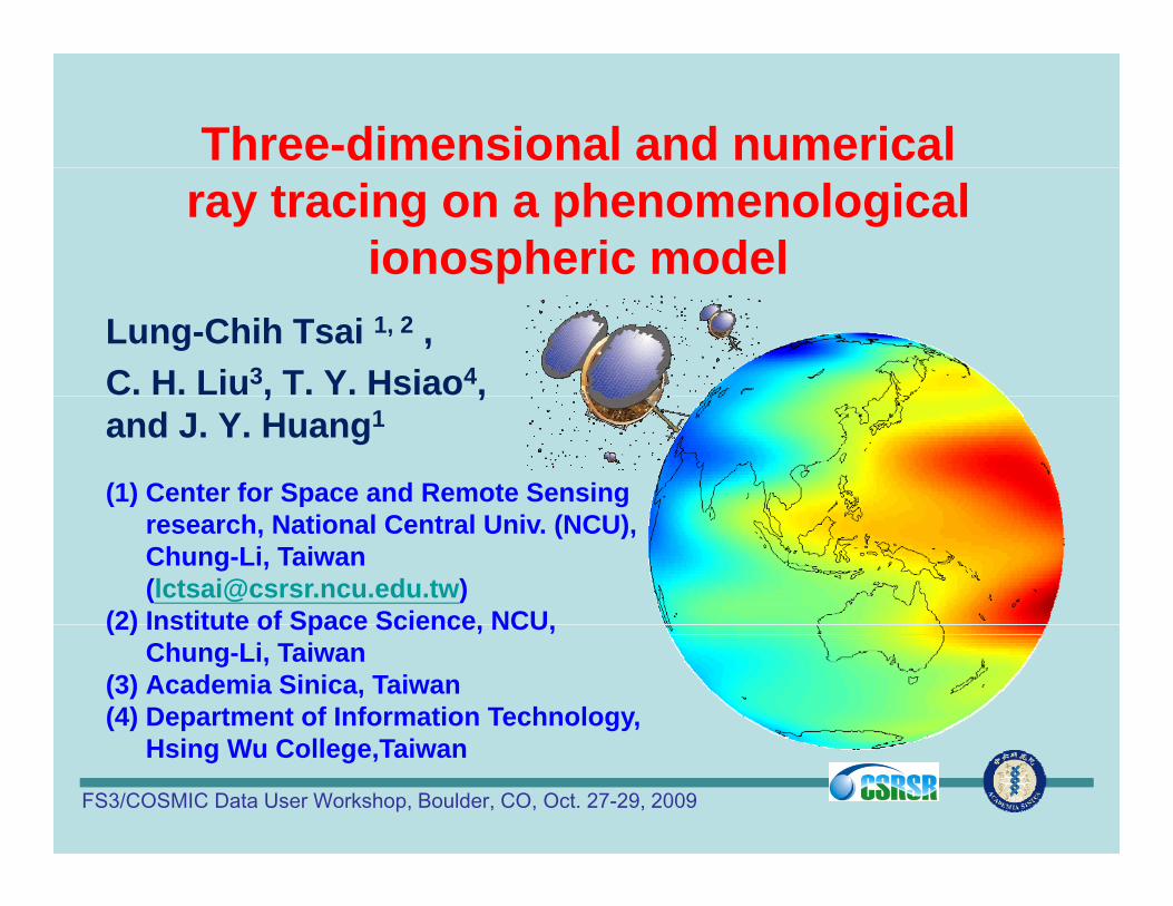
Three-dimensional and numerical ray tracing on a phenomenological

ionospheric modelpLung-Chih Tsai 1, 2 , C. H. Liu3, T. Y. Hsiao4, , ,and J. Y. Huang1

(1) Center for Space and Remote Sensing research, National Central Univ. (NCU), Chung-Li, Taiwan (lctsai@csrsr.ncu.edu.tw)

(2) Institute of Space Science NCU(2) Institute of Space Science, NCU, Chung-Li, Taiwan

(3) Academia Sinica, Taiwan(4) Department of Information Technology,

H i W C ll T iHsing Wu College,Taiwan

FS3/COSMIC Data User Workshop, Boulder, CO, Oct. 27-29, 2009

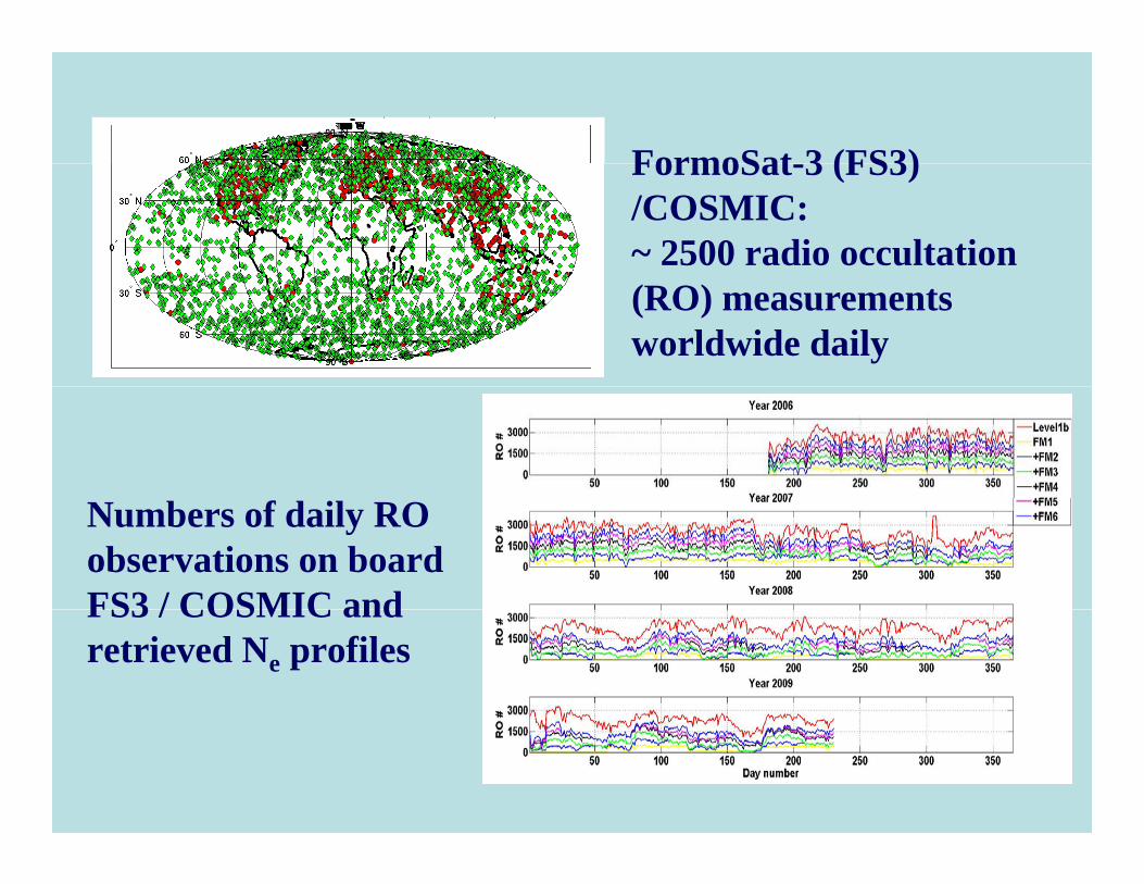
FormoSat 3 (FS3)FormoSat-3 (FS3) /COSMIC: ~ 2500 radio occultation (RO) measurementsworldwide daily

Numbers of daily RO observations on board FS3 / COSMIC andFS3 / COSMIC and retrieved Ne profiles

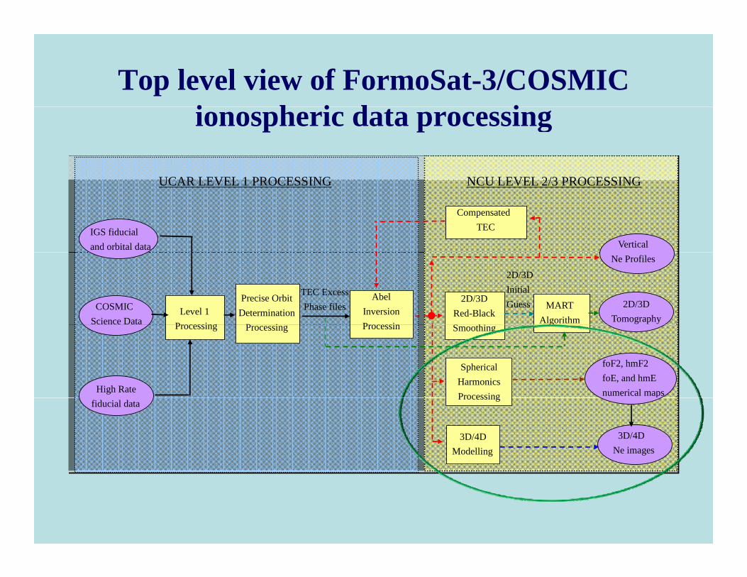
Top level view of FormoSat-3/COSMIC i h i d iionospheric data processing

UCAR LEVEL 1 PROCESSING NCU LEVEL 2/3 PROCESSING

IGS fiducial and orbital data

Compensated TEC

Vertical

UCAR LEVEL 1 PROCESSING NCU LEVEL 2/3 PROCESSING

COSMIC Science Data

Level 1 Processing

Precise Orbit Determination

P i

Abel Inversion Processin

2D/3D Red-Black S hi

MART Algorithm

Ne Profiles

2D/3D Tomography

TEC ExcessPhase files

2D/3DInitial Guess

High Rate

Processing Processing Processin

Spherical Harmonics Processing

Smoothingg

foF2, hmF2 foE, and hmE numerical maps

fiducial data Processing

3D/4D Modelling

3D/4D Ne images

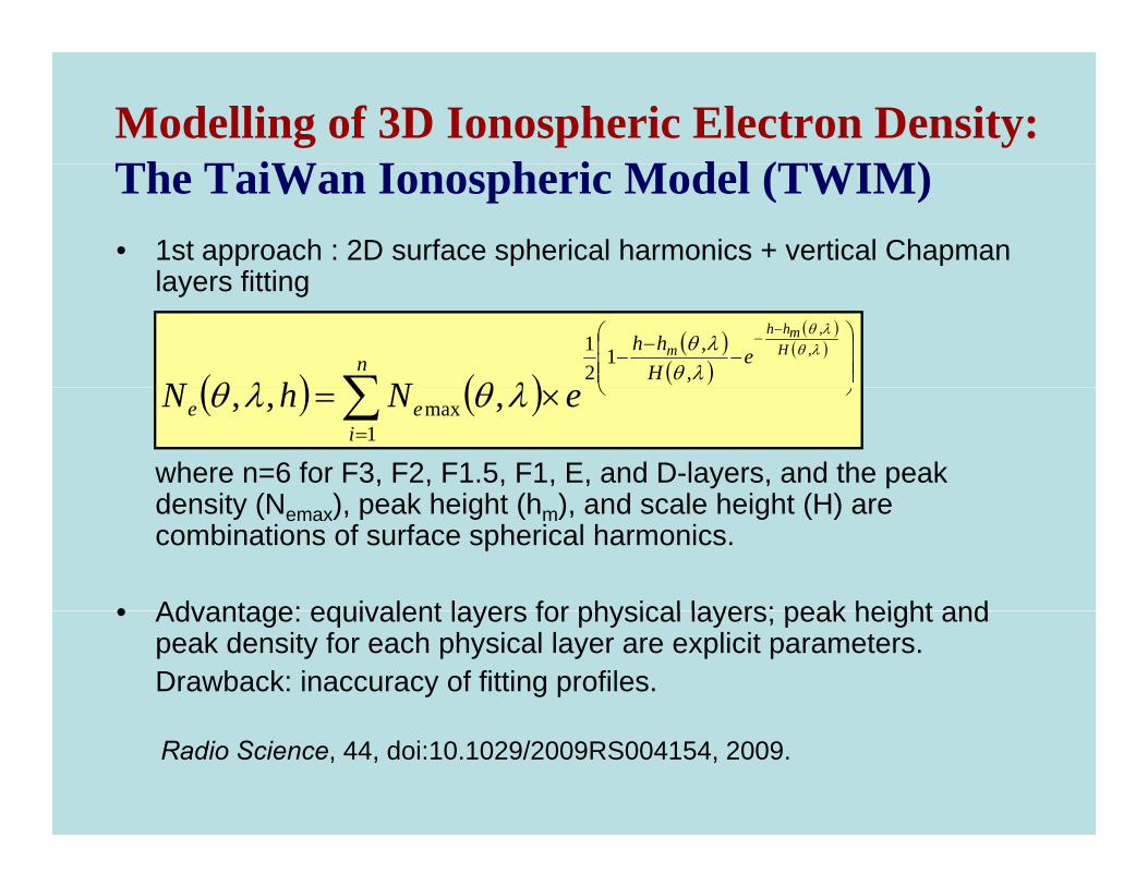
Modelling of 3D Ionospheric Electron Density:Th T iW I h i M d l (TWIM)The TaiWan Ionospheric Model (TWIM)• 1st approach : 2D surface spherical harmonics + vertical Chapman

l fittilayers fitting

n eHhh H

mhhm

NhN,

,121 ,

,

where n=6 for F3, F2, F1.5, F1, E, and D-layers, and the peak density (N ) peak height (h ) and scale height (H) are

i

ee eNhN1

max ,,,

density (Nemax), peak height (hm), and scale height (H) are combinations of surface spherical harmonics.

• Advantage: equivalent layers for physical layers; peak height and• Advantage: equivalent layers for physical layers; peak height and peak density for each physical layer are explicit parameters.Drawback: inaccuracy of fitting profiles.

Radio Science, 44, doi:10.1029/2009RS004154, 2009.

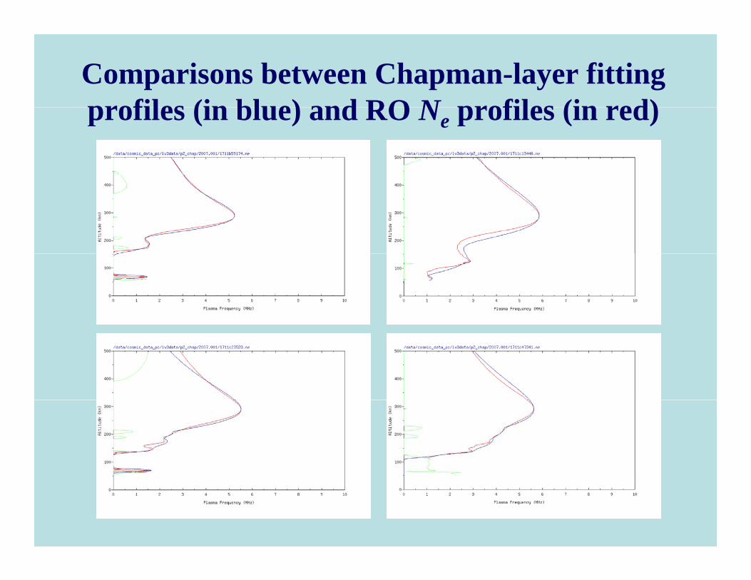
Comparisons between Chapman-layer fitting profiles (in blue) and RO N profiles (in red)profiles (in blue) and RO Ne profiles (in red)

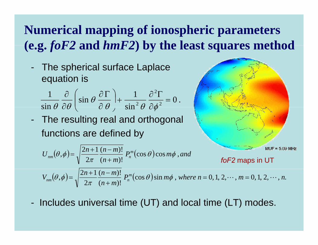
Numerical mapping of ionospheric parameters (e g foF2 and hmF2) by the least squares method(e.g. foF2 and hmF2) by the least squares method

- The spherical surface Laplace ti iequation is

.0sin

1sinsin

12

2

2

- The resulting real and orthogonal

functions are defined by

sinsin

y

,coscos)!()!(

212, andmP

mnmnnU m

nnm

foF2 maps in UT

I l d i l ti (UT) d l l ti (LT) d

.,,2,1,0,,2,1,0,sincos)!()!(

212, nmnwheremP

mnmnnV m

nnm

- Includes universal time (UT) and local time (LT) modes.

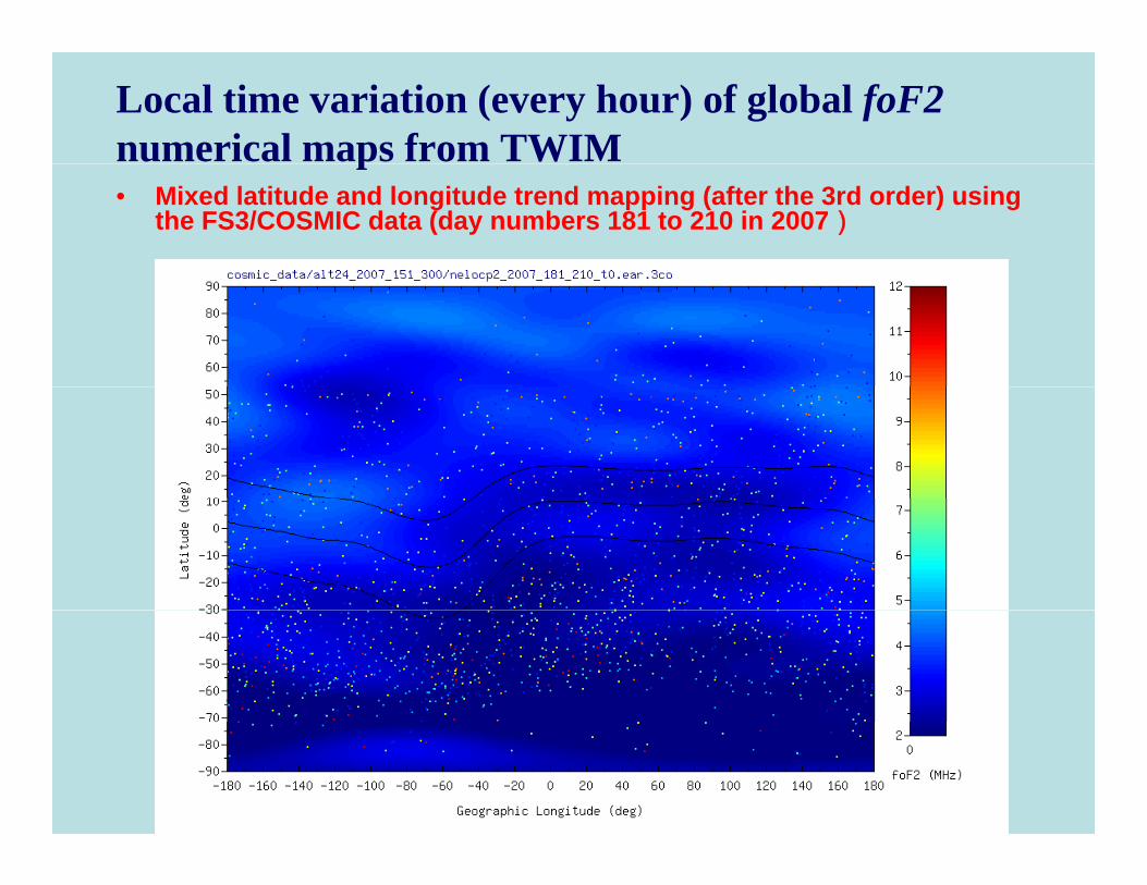
Local time variation (every hour) of global foF2numerical maps from TWIMp• Mixed latitude and longitude trend mapping (after the 3rd order) using

the FS3/COSMIC data (day numbers 181 to 210 in 2007）

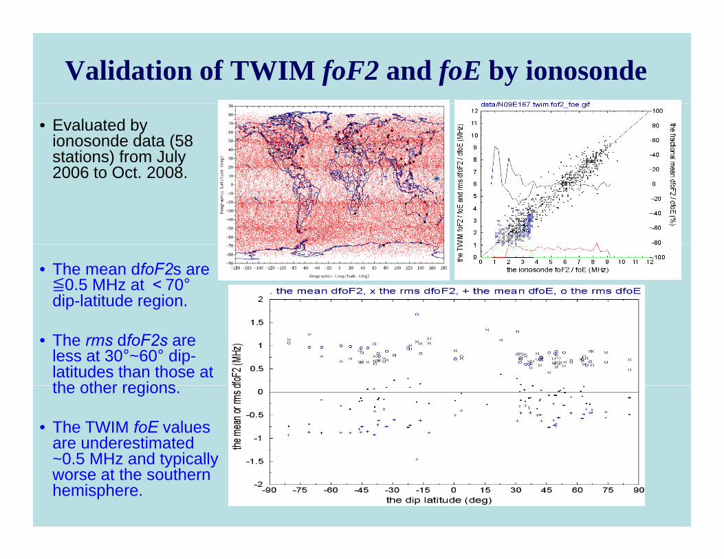
Validation of TWIM foF2 and foE by ionosonde

• Evaluated by ionosonde data (58 stations) from July 2006 to Oct 20082006 to Oct. 2008.

• The mean dfoF2s are 0.5 MHz at ＜70°

dip-latitude region.

• The rms dfoF2s are less at 30°~60° dip-latitudes than those at the other regionsthe other regions.

• The TWIM foE values are underestimated

0 5 MHz and typically~0.5 MHz and typically worse at the southern hemisphere.

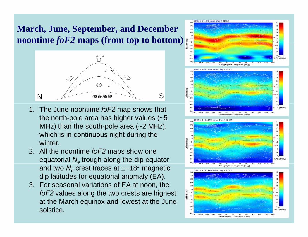
March, June, September, and December noontime foF2 maps (from top to bottom)f p ( p )

磁赤道線 SN

1. The June noontime foF2 map shows that the north-pole area has higher values (~5 MHz) than the south-pole area (~2 MHz), which is in continuous night during thewhich is in continuous night during the winter.

2. All the noontime foF2 maps show one equatorial Ne trough along the dip equator e g gand two Ne crest traces at ~18 magnetic dip latitudes for equatorial anomaly (EA).

3. For seasonal variations of EA at noon, the foF2 values along the two crests are highestfoF2 values along the two crests are highest at the March equinox and lowest at the June solstice.

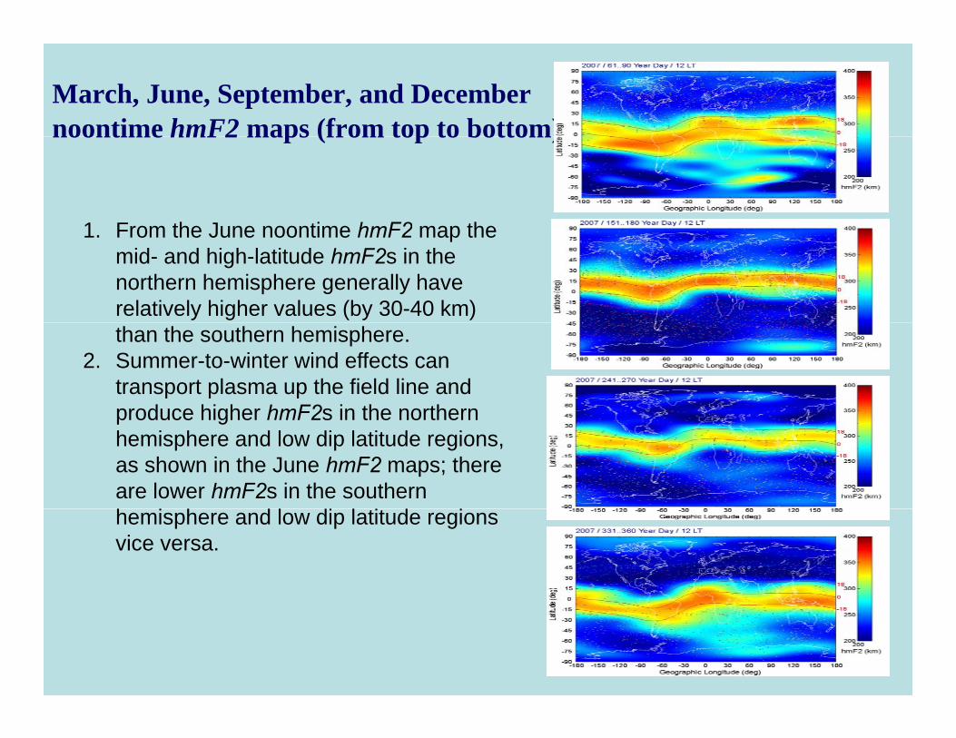
March, June, September, and December noontime hmF2 maps (from top to bottom)noontime hmF2 maps (from top to bottom)

1 From the June noontime hmF2 map the1. From the June noontime hmF2 map the mid- and high-latitude hmF2s in the northern hemisphere generally have relatively higher values (by 30-40 km) than the southern hemisphere.

2. Summer-to-winter wind effects can transport plasma up the field line and produce higher hmF2s in the northernproduce higher hmF2s in the northern hemisphere and low dip latitude regions, as shown in the June hmF2 maps; there are lower hmF2s in the southern h i h d l di l i d ihemisphere and low dip latitude regions vice versa.

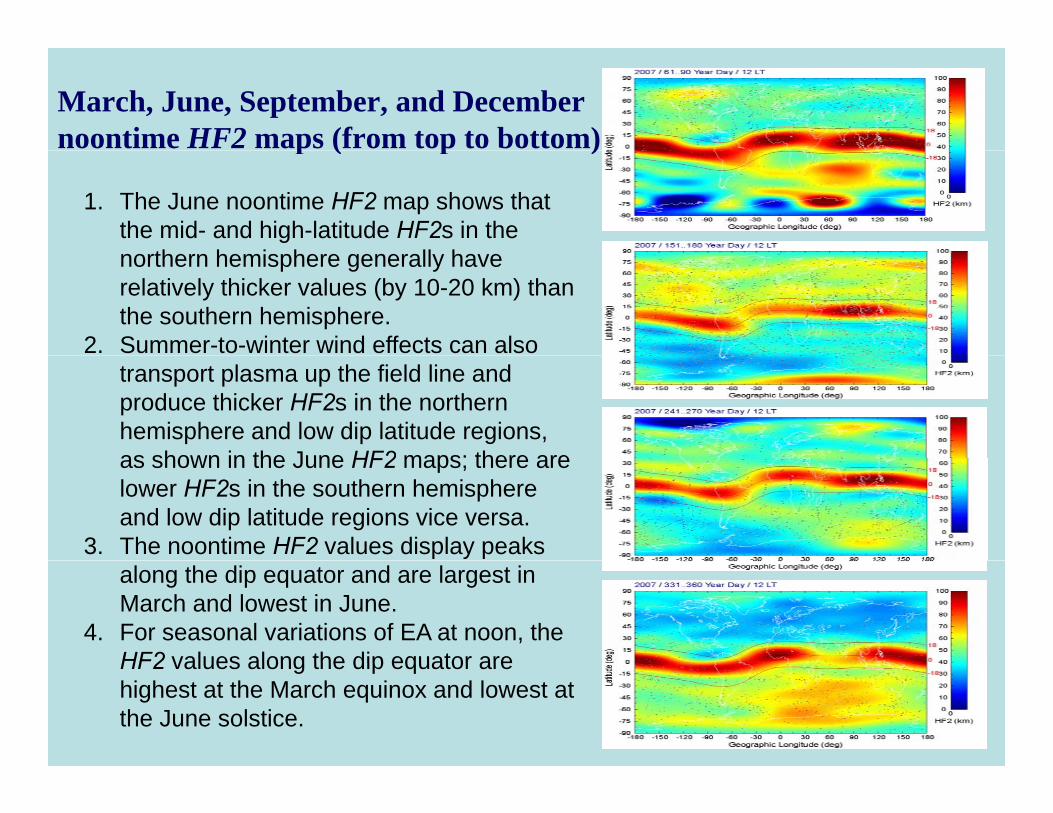
March, June, September, and December noontime HF2 maps (from top to bottom) p ( p )

1. The June noontime HF2 map shows that the mid- and high-latitude HF2s in the

th h i h ll hnorthern hemisphere generally have relatively thicker values (by 10-20 km) than the southern hemisphere.

2. Summer-to-winter wind effects can also transport plasma up the field line and produce thicker HF2s in the northern hemisphere and low dip latitude regions, as shown in the June HF2 maps; there areas shown in the June HF2 maps; there are lower HF2s in the southern hemisphere and low dip latitude regions vice versa.

3. The noontime HF2 values display peaks along the dip equator and are largest in March and lowest in June.

4. For seasonal variations of EA at noon, the HF2 values along the dip equator areHF2 values along the dip equator are highest at the March equinox and lowest at the June solstice.

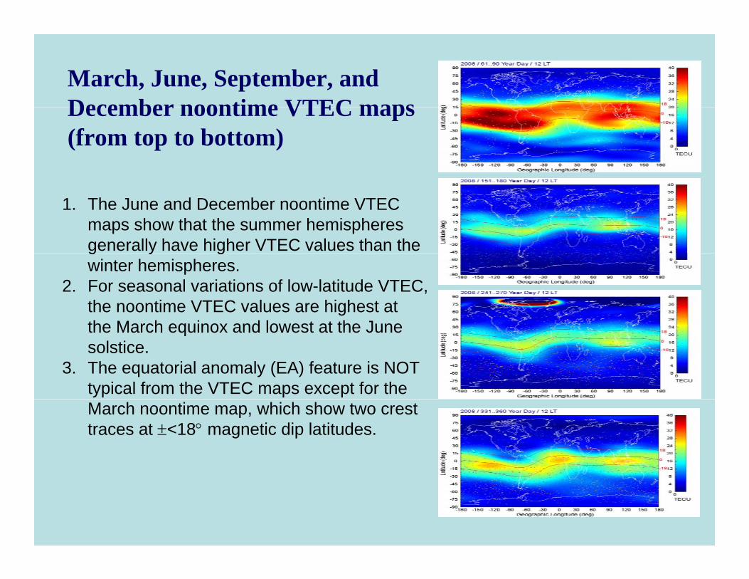
March, June, September, and December noontime VTEC mapsDecember noontime VTEC maps (from top to bottom)

1. The June and December noontime VTEC maps show that the summer hemispheres generally have higher VTEC values than the g y gwinter hemispheres.

2. For seasonal variations of low-latitude VTEC, the noontime VTEC values are highest at the March equinox and lowest at the Junethe March equinox and lowest at the June solstice.

3. The equatorial anomaly (EA) feature is NOT typical from the VTEC maps except for the March noontime map, which show two crest traces at <18 magnetic dip latitudes.

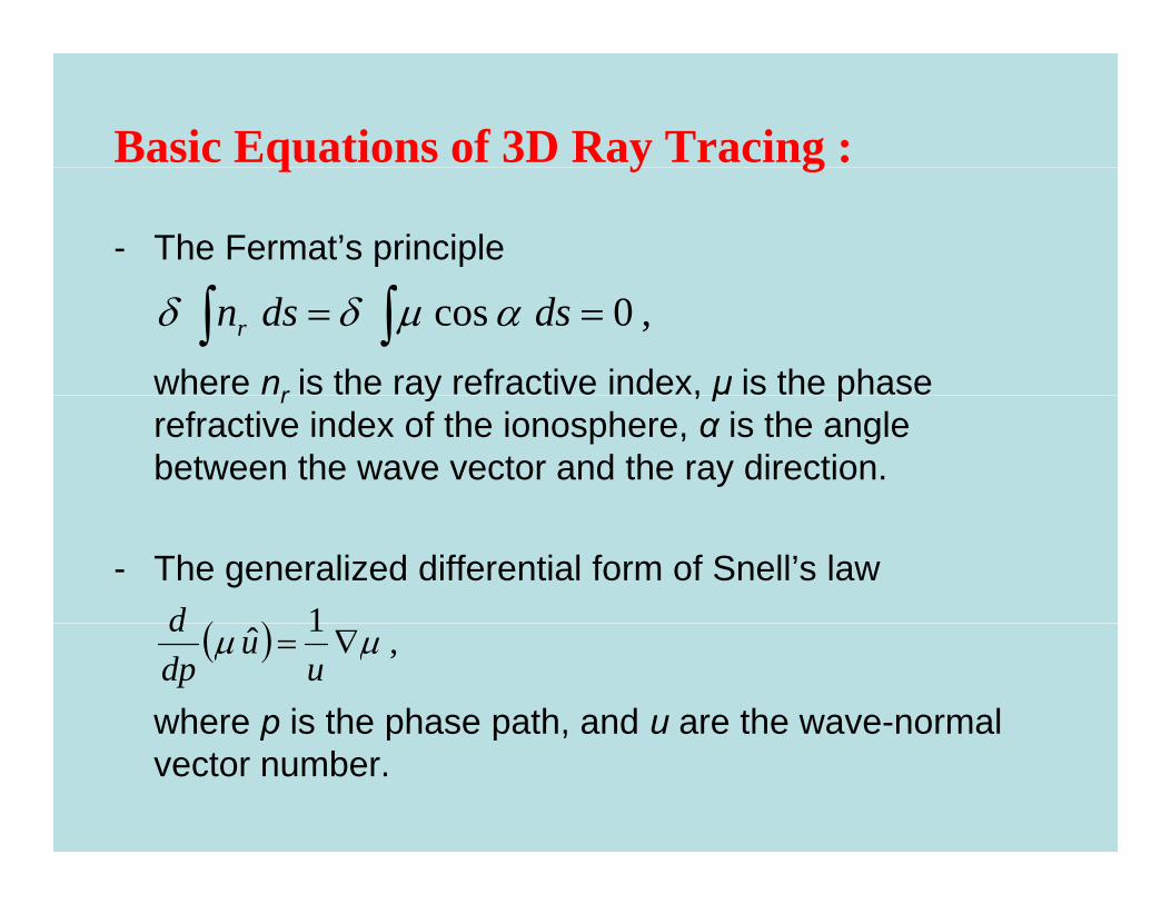
Basic Equations of 3D Ray Tracing :q y g

- The Fermat’s principle

where nr is the ray refractive index, μ is the phase ,0cos dsdsnr

r y , μ prefractive index of the ionosphere, α is the angle between the wave vector and the ray direction.

- The generalized differential form of Snell’s law

1d

where p is the phase path, and u are the wave-normal

,1ˆ u

udpd

p p p ,vector number.

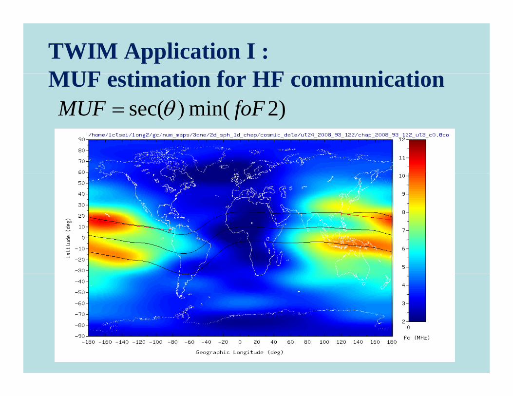
TWIM Application I : MUF ti ti f HF i tiMUF estimation for HF communication

)2min(sec( foFMUF

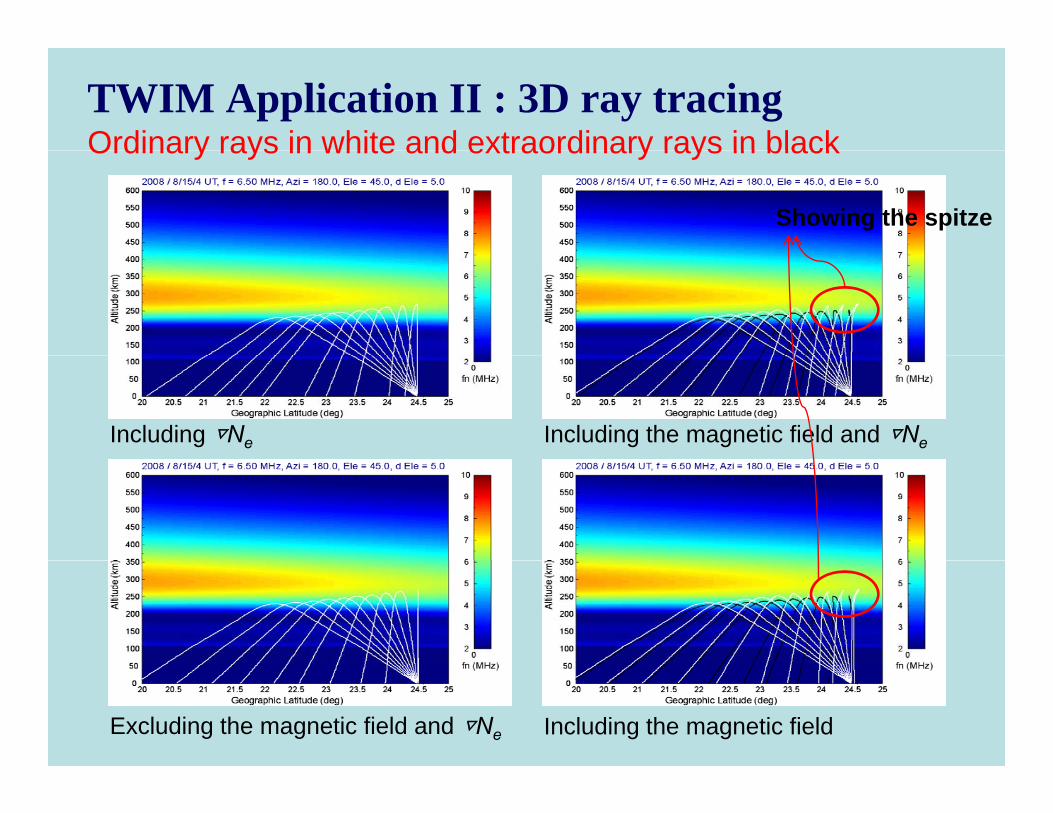
TWIM Application II : 3D ray tracingOrdinary rays in white and extraordinary rays in blackOrdinary rays in white and extraordinary rays in black

Showing the spitze

Including the magnetic field and ▽NeIncluding ▽Ne

Including the magnetic fieldExcluding the magnetic field and ▽Ne

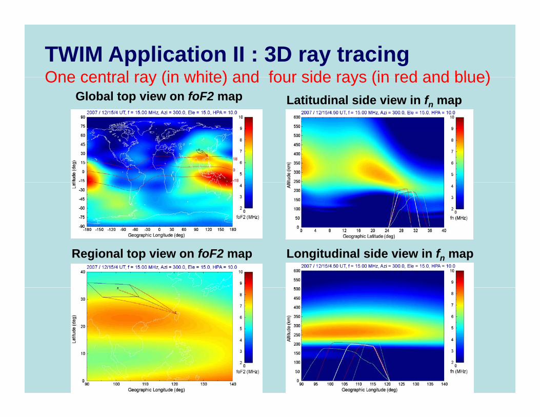
TWIM Application II : 3D ray tracingOne central ray (in white) and four side rays (in red and blue)

Global top view on foF2 map Latitudinal side view in fn map

One central ray (in white) and four side rays (in red and blue)

Regional top view on foF2 map Longitudinal side view in fn map

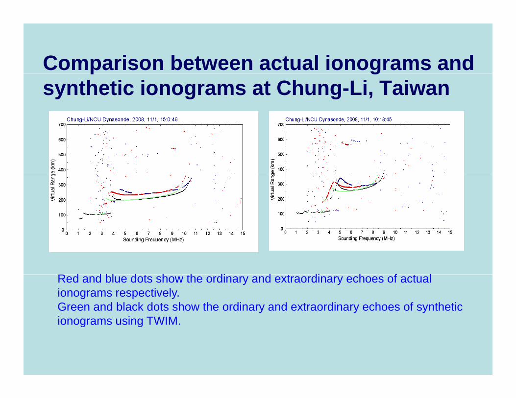
Comparison between actual ionograms and p gsynthetic ionograms at Chung-Li, Taiwan

R d d bl d t h th di d t di h f t lRed and blue dots show the ordinary and extraordinary echoes of actual ionograms respectively. Green and black dots show the ordinary and extraordinary echoes of synthetic ionograms using TWIM.ionograms using TWIM.

Final remarksFinal remarks• FormoSat-3/COSMIC has become a promising program for monitoring

the large-scale global ionosphere.g g p

• A 3D approach using vertical Chapman layers and surface spherical harmonics for modeling variations of ionospheric Ne have beenharmonics for modeling variations of ionospheric Ne have been proposed and implemented to be the TaiWan Ionospheric Model (TWIM).

• A numerical and stepped ray-tracing method on the TaiWan Ionospheric Model (TWIM) has been implemented including the Earth’s magnetic field and N gradient effectsEarth s magnetic field and Ne gradient effects.

Future works• The predictions of TWIM• The predictions of TWIM.