QUANTIFICATION OF UNCERTAINTY

IN LIFE CYCLE ANALYSIS

By

AMANINDER SINGH GILL

A thesis submitted in partial fulfillment of

the requirements for the degree of

MASTER OF SCIENCE IN MECHANICAL ENGINEERING

WASHINGTON STATE UNIVERSITY

School of Mechanical and Materials Engineering

MAY 2014

ii

To the faculty of Washington State University:

The members of the committee appointed to examine the

thesis of AMANINDER SINGH GILL find it satisfactory and recommend that

it be accepted.

_________________________________

Gaurav Ameta, Ph.D., Chair

__________________________________

Robert F. Richards, Ph.D.

___________________________________

Charles Pezeshki, Ph.D.

iii

ACKNOWLEDGEMENT

I cannot express enough thanks to my advisor for their continued support and

encouragement. I want to thank Dr. Ameta for providing me with enriching

learning opportunities during the course of my study.

I would not have been able to accomplish this project without the financial and

emotional support from my parents. They have been a continuous source of

encouragement. Without them, I would never have been able to make it to graduate

school.

I also express my heartfelt gratitude to all the peers I came across during the course

of my studies at Washington State University.

iv

QUANTIFICATION OF UNCERTAINTY

IN LIFE CYCLE ANALYSIS

Abstract

by Amaninder Singh Gill, M.S.

Washington State University

May, 2014

Chair: Gaurav Ameta

The aim of this thesis is to accumulate uncertainty in Life Cycle Analysis (LCA).

LCA is a technique to identify environmental impacts of processes and thereby

product’s life cycle from material extraction to product disposal. An important

aspect of LCA is that it is not always feasible to measure the environmental impact

of individual processes occurring during a product life cycle. Therefore, data from

similar processes from different time frame, different geographic location, different

process technology, etc., is utilized. Such approximate data introduces

uncertainties in the results of LCA.

The uncertainty in LCA is usually a mix of two types of uncertainty; aleatory,

arising from natural process variability, and epistemic, arising due to lack of

information regarding the process and related environmental impact. Aleatory

v

uncertainty has been applied and implemented in LCA software using Monte-Carlo

Simulations. To the best of our knowledge, epistemic uncertainty or mixed

uncertainty has not been applied in a LCA

In order to apply epistemic or mixed uncertainty in LCA, a model is developed

based on evidence theory and random sets. A specific variation of evidence theory,

called Dempster-Shafer theory is utilized in creating the model. Random sets help

in quantifying uncertainties from multiple data sources regarding the same process.

These sets may have statistical distribution and will have belief and plausibility

functions associated with them. In the model the random sets with distributions,

belief and plausibility functions from multiple processes in the product life cycle

are accumulated to provide statistical distribution and mean for the resultant

environmental impact.

To apply this theory, a test case of TV Remote Control was taken. As a first step,

the environmental impacts obtained from product’s LCA (environmental impacts)

of individual life cycle stage were modeled with epistemic uncertainty as random

sets. The uncertainties were then discretized into corresponding belief and

plausibility functions. Then, a cumulative distribution was created from the

random sets to accumulate the results. Results in terms of statistical variation and

mean can then be obtained from the accumulated cumulative distribution functions.

vi

TABLE OF CONTENTS

Page

ACKNOWLEDGEMENTS…………………………………………………….…III

ABSTRACT……………………………………………………………………....IV

LIST OF FIGURES……………………………………………………………….VI

CHAPTER

1. INTRODUCTION……………………………………………………….…….1

1.1 Life Cycle Analysis …………………………………………………….1

1.2 Goal Definition and Scoping……………………………………………3

1.3 Life Cycle Inventory…………………………………………….………5

1.4 Life Cycle Impact Assessment………………………………………...9

1.5 Uncertainty…………………………………………………………….10

1.6 Sources of Uncertainty………………………………………………...10

1.6.1 Types of Uncertainty………………………………………………...10

1.6.2 Quantification and Accumulation of Uncertainty………………..….12

vii

1.7 Problem Statement……………………………………………………..12

1.8 Outline………………………………………………………………….13

2. REVIEW OF LITERATURE…………………………………………………..14

2.1 Uncertainty in LCA……………………………………………………14

2.1.1 Epistemic Uncertainty and Aleatory Uncertainty……………………15

2.2.2 Sources of Epistemic Uncertainty…………………………………..16

2.2.3 Sources of Aleatory Uncertainty…………………………………….17

2.3 Research Efforts on Aleatory and Epistemic Uncertainty…………….21

2.4 Need of Research in Mixed Uncertainty in LCA……………………...31

3. METHODOLOGY……………………………………………………………..32

3.1 Introduction…………………………………………………………….32

3.2 Deficiencies in Classical Probability Theory………………………….32

3.3 Quantifying Uncertainty……………………………………………….36

3.3.1 Data Sources………………………………………………………….37

3.3.2 Random Sets…………………………………………………………37

3.3.3 Evidence Model………………………………………………………39

viii

3.3.4 Statistical Methods…………………………………………………...45

3.3.5 Aggregation Uncertainty…………………………………………….46

3.4 Algorithm…………………………...………………………………….47

3.4.1 LCA……………………………………………………………..……48

3.4.2 Outputs…………………………………………………….…………48

3.4.3 Uncertainty………………………………………………….………. 49

3.4.4 Random Sets in Conjunction with Dempster Shafer Theory………...49

3.4.5 Six Uncertainties and Expert Opinions.……………………………...49

3.4.6 Belief and Plausibility………………………………………………..50

3.4.7 CDF………………………………………………………………..…50

3.4.8 Conclusion…………………………………………………………....51

4. CALCULATIONS………………………………………..……………………52

4.1 Input Data Sets…………………………………………………………52

4.2 Creating Random Sets and Belief and Plausibility Functions…….…...53

4.2.1 Manufacturing Phase…………………………………………………56

ix

4.2.2 Product Delivery Phase………………………………………………57

4.2.3 Disposal Delivery Phase……………………………………………...58

4.2.4 Use Phase…………………………………………………………….59

4.5 Mean and Variance……………………………………………………..61

4.6 Conclusion……………………………………………………………...61

5. CONTRIBUTIONS AND FUTURE WORK………………………………….62

5.1 Contributions…………………………………………………………...62

5.2 Future Work……………………………………………………………63

6. REFERENCES…………………………………………………………………65

x

LIST OF FIGURES

Figure 1: An overview of LCA Framework……………………………………….3

Figure 2: Laying out boundary systems while scoping…………………………….4

Fig 3.1 A schematic of the tools used to quantify uncertainty……………………36

Fig 3.2: Algorithm for quantifying uncertainty…………………………………...47

Fig 4.1 CDF for Manufacturing Phase……………………………………………57

Fig 4.2 CDF for Product Delivery Phase…………………………………………58

Fig 4.3 CDF for Disposal Delivery Phase……………………..…………………59

Fig 4.4 CDF for Use Phase………………………………………………………60

xi

LIST OF TABLES

Table 4.1: Output from LCA of TV remote control………………………………53

Table 4.2 Discretization of Manufacturing Phase output ………………………...56

Table 4.3 Discretization of Product Delivery Phase output………………………57

Table 4.4 Discretization of Disposal Delivery Phase output……………………...58

Table 4.5 Discretization of Use Phase output……………………………………59

Table 4.6 Average and Standard Deviation of CDF……………………………..61

1

CHAPTER 1

INTRODUCTION

Due to global warming issues, sustainable design, manufacturing, use and disposal

of products is being considered by design and manufacturing firms everywhere.

Mitigating environmental impacts from all the processes during the entire life of a

product is one important aspect being considered in design of sustainable products.

In the design stage, planning related all other stages of product life is performed. It

is also stipulated that almost 70% of the products cost is incurred based on the

decisions made in the design stage [1]. Therefore, it is pertinent to consider various

design choices in order to estimate and mitigate environmental impacts of these

choices. One of the common methods of estimating environmental impacts at the

end of the design stage is called Life-Cycle Analysis.

1.1 Life Cycle Analysis

Environmental Protection Agency (EPA) defines Life Cycle Analysis ( LCA ) as

technique to assess the environmental aspects and potential impacts associated

with a product, process, or service, by:

• Compiling an inventory of relevant energy and material inputs and environmental

releases

2

• Evaluating the potential environmental impacts associated with identified inputs

and releases

• Interpreting the results to help decision-makers make a more informed decision.”

[1]

LCA is conduct utilizing four major steps. The first one is called Goal Definition

and Scoping. In this step, the product or activity being analyzed is defined and

system boundaries are specified. System boundaries pertain to what all processes

will be included and analyzed in the LCA study. The next step is Inventory

Analysis. In this step, an inventory of all the materials and energy being used in all

the products and processes is . The next step is Impact Assessment. In this step, all

the environmental impacts caused by the materials and processes are calculated.

These impacts are usually in the form of equivalent CO2 produced and also in the

form of harmful gases and water pollutants. The last and final step in the LCA is

Interpretation. In this step, the results of the impact assessment are evaluated and

interpreted. Figure 1 shows all the four steps in LCA [1] and demonstrates the flow

of information between these steps. In the next few paragraphs, all the steps

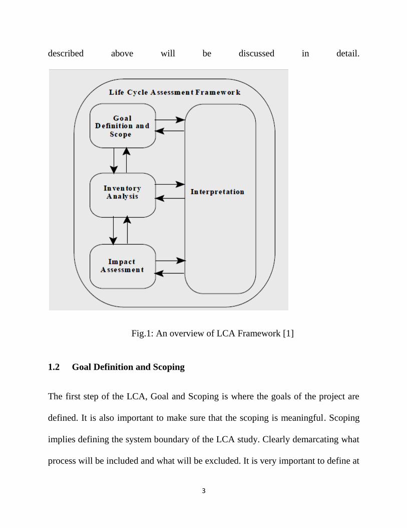
3

described above will be discussed in detail.

Fig.1: An overview of LCA Framework [1]

1.2 Goal Definition and Scoping

The first step of the LCA, Goal and Scoping is where the goals of the project are

defined. It is also important to make sure that the scoping is meaningful. Scoping

implies defining the system boundary of the LCA study. Clearly demarcating what

process will be included and what will be excluded. It is very important to define at

4

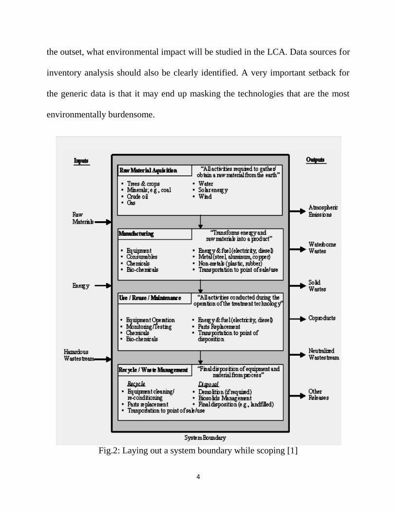
the outset, what environmental impact will be studied in the LCA. Data sources for

inventory analysis should also be clearly identified. A very important setback for

the generic data is that it may end up masking the technologies that are the most

environmentally burdensome.

Fig.2: Laying out a system boundary while scoping [1]

5

The scope definition must also ensure that the quantity of the two products being

compared is the same. The most important stages that are usually defined in the

scope definition are raw materials acquisition, manufacturing, use phase, supply

chain, maintenance and end-of-life. Scope definition also implies defining a

functional unit that will be used to evaluate the impact. Functional unit is basically

a unit of measure. For an example of LCA of a coffee machine, a functional unit

can be defined as a cup of coffee, 1 run of the coffee machine or the entire life of 1

coffee machine.

1.3 Life Cycle Inventory

The second step of the LCA is Inventory Analysis. Life Cycle Inventory (LCI) is a

process of quantifying energy and raw material requirements, atmospheric

emissions, waterborne emissions, solid wastes, and other releases for the entire life

cycle of the product, process and activity [1]. There are 4 important sub-stages of

LCI: Develop the flow diagram of the processes being evaluated, develop data

collection plan, collect data, evaluate and report results.

Flow diagrams depict all the individual steps (called subsystems) that have been

included in the analysis. Which steps will be included in the diagram is decided by

goal and scope definition. To quantify the amount of materials and energy being

used by each of the step, data must be collected from the manufacturing facility

6

itself. Data Quality Indicators (DQIs) also need to be included with the data so that

the analysts can get an idea about the accuracy, precision, representativeness and

completeness of the data.

In the second step, the data collection plan needs to be developed. Initially, the data

quality goals have to be defined. An accurate example of this would be that using

data which is geographically, temporally and technologically nearest to the

situation being analyzed.

The types of data and sources from which the data can be obtained has been

specified by the Environmental Protection Agency (EPA) [5]. The types of data

include data that can be measured, modeled, sampled and obtained from a vendor.

Logically, the next step is data collection. Data collection can be done by a lot of

different methods – site visits and direct contact with the experts are considered the

most accurate ways of collecting data. There are secondary ways of collecting data

i.e. obtain non site specific inventory data. Every process is a stream of materials

and energy coming in and going out. There are some ISO rules for collecting data

to ensure there is a complete and accurate collection of data. Besides that, there are

also some thumb rules for data collection. All the relevant data must be included,

no matter how minor the quantity seems. The term relevant data refers to all the

data that can be included in the goal and scope definition. Apart from the matter

7

coming in and out, there is also energy being used in all the processes. To account

for all the energy being used, it can be divided into three categories for the purpose

of quantifying it. These categories are: process, transportation and energy of the

material resources.

Process Energy can be understood as the energy used to perform the various

subsystem items like heat exchangers, pumps, etc. Transport Energy can be

thought of as the energy used to transport all the materials from one place to

another.

Since the processes do take in inputs, it is very apparent that there will be some

outputs as well. There are three categories of environmental releases: atmospheric

emission, water borne waste and solid waste. These outputs have been explained in

detail in the following paragraph.

Atmospheric pollution is defined as all the substances released into the air as a

result of the process in question. The amount of atmospheric pollution is reported

in units of weight. The common atmospheric pollutants are oxides of carbon, sulfur

and nitrogen. Some aldehydes, ammonia, lead and organic compounds are also

considered as pollutants.

Waterborne wasted are defined as those unwanted by-products of the process

which are released into a water stream, usually in a liquid or a semi-solid form.

8

The liquids that can typically be considered a waterborne waste are usually defined

by regulatory agencies under specific legislations, such as the Resource

Conservation and Recovery Act. Some of the common waterborne wastes are

suspended solids, dissolved solids, cyanides, fluorides, phosphates and phenols.

Solid wastes are defined as those unwanted by-products of the process which are

released into a water stream in a solid form. Fuel combustion residues, mineral

extraction wastes, and solids from utility air control devices can be common

examples of solid wastes.

The most important outcome of the process and this whole system is the product.

The product can be an outcome of the sub system, which will be the raw material

for the consecutive sub system, or the final product of the whole system.

Another very important part of the Life Cycle is transportation. Transportation

includes all movement of raw material from its initial to its final stages. That

includes shipping the raw material to the manufacturing/processing facility, the

transportations inside the facility and the final transportation of the finished

product form the facility to the market. The transportation is measures as the

distance travelled. Since the total fuel consumption would not just depend on the

distance moved but also the amount of weight/volume moved too; the calculations

are based off of weight (volume)-distance units. It must be kept in mind that there

9

can certainly be overlaps in calculating the total weight transported and distance

travelled.

Other very important factors that have to be accounted for in the LCI are the

temporal and geographic factors. It is very important that the data being used must

either come from the same temporal and geographic locations to ensure an accurate

analysis. If it is not possible to get the data from a relevant temporal and

geographic source, some method must be used to compensate for this effect.

1.4 Life Cycle Impact Assessment

Life Cycle Impact Assessment is defined as the phase in which the evaluation of

potential human health and environmental impacts of the process undertaken are

quantified and analyzed. Impacts are usually categorized as global, regional and

local. Global impacts include global warming, ozone depletion and resource

depletion. Regional impacts are usually photochemical smog and acidification.

Local impacts are characterized by impact on human health, terrestrial toxicity,

aquatic toxicity, eutrophication, increased land and water use for disposing off

wastes. Impact indicators are calculated as:

Inventory Data × Characterization Factor = Impact Indicators [1]

10

1.5 Uncertainty

Uncertainty in simple terms can be defined as something which is not certain,

hence by definition difficult to define precisely [3]. The sources, types and

definitions of the various uncertainties that can arise in an LCA are discussed in

the sections below. A more detailed study of uncertainty and its effects on LCA

have been discussed in Chapter-2.

1.6 Sources of Uncertainty

Uncertainty can stem from a variety of reasons and the source of uncertainty can

be many. Some of them are listed here. Random error, statistical variation,

linguistic imprecision, variability, inherent randomness and approximation can be

some of the reasons why uncertainty. [2]

1.6.1 Types of Uncertainty

In the course of this study, the uncertainty has been looked at using a very different

criterion. For the purpose of this research, uncertainty can of two types: variability

and imprecision [3]. Variability is defined as a naturally random behavior of a

physical process due to its inherent properties. Such an uncertainty stemming from

variability is also called as aleatory uncertainty. It can also be attributed to random

error or statistical variation. It is always present, but can be minimized.

11

The second type of uncertainty in this study is the one which stems from

imprecision. It arises due to the inherent lack of knowledge of a process. In theory,

it might be possible to measure those specific values, but in reality it is not. Such

an uncertainty which stems form imprecision is called as epistemic uncertainty.

For this study, only the above stated two types of uncertainties will be considered.

But, for the purpose of simplicity, many researchers tend to categorize

uncertainties using specific emphasis on the importance on different issues. Baker

et al. [4] while recognizing the two main types of uncertainties as database

uncertainty, model uncertainty, statistical error, uncertainty in preference and

uncertainty in a future physical system.

Database uncertainty is attributed to differences in calculated environmental

impact value due to geographical and temporal parameters. Model uncertainty can

be attributed to over simplification of models which in turn are no longer capable

of capturing the cause and effect mechanism partly or fully. Statistical error is

attributed to measurement error. Uncertainty in preferences usually arises from the

selection of goal and scope definition. Uncertainty in future physical system can

arise due to lack of knowledge of future material, design failures or human error.

12

1.6.2 Quantification and Accumulation of Uncertainty

Once the sources and types of uncertainty have been identified, it is important to

discuss how we can measure the uncertainty. Measuring uncertainty is also called

quantification [2]. In the simplistic cases, classical tools of probability and

statistics can be used. The target variables, usually database or input variables are

identified and the tools of uncertainty quantification are used on them. Apart from

input variables, database values are also of importance for uncertainty

quantification. Monte Carlo method is also used to quantify uncertainty. The

details of these methods will be discussed in Chapter -2 and the new algorithm will

be discussed in Chapter -3.

1.7 Problem Statement

In LCA, both types of uncertainties are involved. Uncertainty due to imprecision

can be easily quantified and accumulated. But aleatory uncertainty has not yet been

quantified and accumulated in LCA.

The purpose of this study is to (a) create a methodology for utilizing aleatory

uncertainty in LCA (b) demonstrate the application of aleatory uncertainty in LCA

through a case study.

13

1.8 OUTLINE

This chapter describes the need for quantifying uncertainty in LCA. A holistic

review of literature will be done in Chapter – 2. This will examine the techniques

being currently used to quantify uncertainty and their limitations and drawbacks.

Chapter – 3 will consist of the methodology using which this research proposes to

quantify uncertainty. Lastly, Chapter – 4 will consist of all the calculations that

have been undertaken to quantify uncertainty.

14

CHAPTER – 2

REVIEW OF LITERATURE

Uncertainty in Life Cycle Analysis is well known. As stated in the Introduction

chapter, there are various ways to look at uncertainty and define it.

2.1 Uncertainty in LCA

In this chapter, classification of uncertainty will be deal in detail. In addition a

holistic review of literature will be done to see how uncertainty is being handled in

various applications by different authors. As has been discussed before, there are

many kinds of uncertainty, but for the sake of this study, only Epistemic and

Aleatory will be considered as two broad types of uncertainty and all the other

types will be clubbed under these two broad types. Moreover, the nature of

uncertainty and how they are dealt with depends on the context

2.2 Categorization and Characterization of Uncertainty

This section will deal with definitions of the two types of uncertainties and their

mathematical characterization. The advantage of separating the uncertainties into

aleatory and epistemic is that we thereby make clear which uncertainties can be

reduced and which uncertainties are less prone to reduction, at least in the near-

term, i.e., before major advances occur in scientific knowledge. This categorization

15

helps in allocation of resources and in developing engineering models.

Furthermore, better understanding of the categorization of uncertainties is essential

in order to properly formulate risk or reliability problems [28].

2.1.1 Epistemic Uncertainty and Aleatory Uncertainty

The word epistemic derives from the Greek (episteme), which means

knowledge. Thus, an epistemic uncertainty is one that is presumed as being caused

by lack of knowledge (or data). It is mostly associated with derived parameters, i.e.

those parameters which have not been measured directly [28].

The word aleatory derives from the Latin alea, which means the rolling of dice.

Thus, an aleatoric uncertainty is one that is presumed to be the intrinsic

randomness of a phenomenon. Aleatory Uncertainty is associated with measured

that are measured directly [28].

To elaborate on the difference between these two uncertainties, consider the

following example. Let the annual maximum wind velocity be the variable of

interest in design of a tower. The modeler can either consider this quantity as a

basic variable o as an aleatory uncertainty. For representing the variable as an

aleatory uncertainty, the modeler would have to fit a probabilistic sub-model,

possibly selected from a standard recommendation. This will help him/her to

empirically obtained annual maximum wind velocity data. Also, the modeler may

16

choose to use a predictive sub-model for the wind velocity derived from more

basic meteorological data. In that case, the annual wind velocity is a derived

variable of the form Y = gxθg where x denotes the input basic meteorological

variables and gxθg denotes the predictive sub-model of the wind velocity. The

uncertainty in the wind model now is a mixture of aleatory and epistemic model

uncertainties [28].

2.2.2 Sources of Epistemic Uncertainty

In this section the sources of epistemic uncertainty will be discussed. Uncertain

modeling errors, resulting from selection of the physical sub-models, gi(x,θg) i =

1,2,. . . ,m, used to describe the derived variables. Uncertain errors involved in

measuring of observations, based on which the parameters θf and θg are estimated.

These errors specifically pertain to indirect measurement of parameters. Epistemic

uncertainty will also arise from numerical approximations and truncations, which

we could know about in theory, but know little about in practice [28]. Parameter

uncertainties are normally epistemic in nature, because the uncertainty in the

estimation might asymptotically vanish with increasing quantity and quality of

data. In many cases, the amount of additional information to gather, e.g., the

sample size, is a decision problem itself, and usually the optimal decision is one

that leaves some residual parameter uncertainty [28].

17

2.2.3 Sources of Aleatory Uncertainty

Uncertainty also occurs in an aleatory sense. This section will explore the sources

for aleatory uncertainty. In basic random variables X, uncertainty is an inherent

property by virtue of errors that occur in directly measured values. Uncertainty will

also arise from statistical uncertainty in the estimation of the parameters θf of the

probabilistic sub-model. Statistical uncertainty has also to be factored in during the

estimation of the parameters θg of the physical sub-models. Model errors will also

contribute to aleatory uncertainty occurring in basic variables [28]. The parameters

(θg, ΣE) of the physical sub-models and θf of the distribution sub-model are

estimated by statistical analysis of observed data. Specifically, (θg, ΣE) are

estimated based on pairwise observations of Y and X, and θf are estimated based

on observations of X. The preferred approach is the Bayesian analysis which

allows incorporation of prior information on the parameters, possibly in the form

subjective expert opinion. The uncertainty in the parameter estimates, often called

statistical uncertainty or aleatory uncertainty [28].

2.1.3 Characterization of Uncertainty

Aleatory and Epistemic Uncertainties seldom occur separately. They occur

together and have to be characterized together. Consider this probabilistic

18

model Y = gxθg. In this model, E accounts for the uncertain effects of the

missing variables z as well as the potentially inaccurate form of the model. In this

sense, the uncertainty E is categorized as at least partly epistemic and gxθg) is

categorized as at least partly aleatory. However, the limited state of scientific

knowledge does not allow us to further refine the model [28].

A generic review of literature shows that the presence of uncertainty is

acknowledged by most researchers working on LCA. For this research,

several research papers that talk about various approaches to understand

and account for uncertainty in LCA were reviewed.

One of the most seminal works in quantification of uncertainty has been

done by M.A.J. Huijbregts as part of his doctoral research [6]. Huijbregts’

work deals with uncertainty and variability. By uncertainty he means

epistemic uncertainty and by variability he means aleatory uncertainty. His

work deals with uncertainty caused by parameters, choices and model.

Typically, a preset distribution is used to quantify uncertainty. The

downside of using a preset distribution is that it leads to quantifying a very

large amount of uncertainty, which is not at all helpful in making a

decision.

19

Another papers reviewed was authored by Anna E. Bjorklund [7]. In this

paper, the author has traced the sources of uncertainty to be Data

Inaccuracy, Data Gaps, Unrepresentative Data, Model Uncertainty, and

Uncertainty due to choices, spatial variability, temporal variability,

variability between sources and objects, epistemological uncertainty,

mistakes and estimation of uncertainty. In the next section, the author talks

about qualitative and quantitative ways to improve data quality and

availability. The author suggests using acceptable ISO standards. Another

very important quantitative suggestion made by the author is to use those

databases in which data is provided in such a way that the provider reveals

proprietary information. DQGs can also be used to describe the desirable

qualities in the data. As per ISO standards it is mandatory for DQG to

specify uncertainty of information. In addition to DQGs, DQIs (Data

Quality Indicators) can be used to ensure the data quality. DQI is

characterized by accuracy, bias, completeness, precision, uncertainty,

amongst others. The author further suggests using Validation of Data and

Parameter Estimation Techniques to minimize and remove uncertainty.

Also, additional measurements, higher resolution models and critical review

would also further help to reduce uncertainty in the data set. Apart from

20

these measures, sensitivity and uncertainty analysis can help in estimation

of effects on a study of uncertainty that is carried out using a set of data and

algorithms. Sensitivity is defined as “the influence that one parameter has

on the value of the other parameter, both of which may be either continuous

or discrete”. The author has also listed several kind of sensitivity analysis

that can be performed so that the effect of assumptions, methods and data

can be understood. Theses analysis can be one-way, scenario, factorial

design (multivariate analysis), ratio sensitivity and critical error factor.

Further, an uncertainty importance analysis can also be carried out to see

how the parameter uncertainty contributes to the total uncertainty of the

result. The uncertainty importance analysis can be qualitative or

quantitative in nature. The higher the uncertainty of a parameter the more

important is it to address it.

Another important study to document the various approaches undertaken to

estimate uncertainty quantification in LCA has been done by Heijungs et al

[19]. The authors have identified parameter analysis, sampling methods and

analytical methods to deal with uncertainty. In sampling methods, the

authors have identified using distributions ( normal, lognormal etc ) used to

sample input parameters. Many researchers have also used Monte Carlo

21

analysis to tackle uncertainty. Also, input, process and output uncertainties

have been dealt with separately by most researchers.

2.3 Research Efforts on Epistemic and Aleatory Uncertainty

In this section we will go over the various types of uncertainties, Epistemic,

Aleatory or both, that have been dealt with by the respective researchers.

Various authors have also worked on quantifying uncertainty via

mathematical models. One such study is done by Huijbregts et al [8].The

author classified data uncertainty as data inaccuracy and lack of specific

data. Lack of Data is further classified as Data gaps and Unrepresentative

data. The author specifically states that setting the unknown parameter to

zero while doing an LCI makes the LCA biased. The author also

emphasizes that the inter-processes must also be taken into account either

by using the original data. Substitution of lesser known material data with

better known analogous material data is also acceptable to a certain degree.

The author further suggests that keeping track of process outputs is very

important. Although law of mass balance can be used to predict outputs,

using this technique can result in underestimation of pollutants which are

created as a by-product of chemical reactions in particular. The author has

also talked about a systematic bias that gets introduced in an LCI when

22

unrepresentative data is used. To deal with this bias it is suggested that

uncertainty factors (UF) be for non-representative data be included in LCIs.

This UF works just like assessment factor in risk analysis techniques. The

next big factor inducing uncertainty is Data Inaccuracy. Data inaccuracy is

simply caused by errors in measurement. Fuzzy logic and stochastic

modeling (like Monte Carlo) are one of the most popular methods to deal

with uncertainty arising out of data inaccuracy. The author recommends

that before doing any kind of stochastic modeling, the researcher must first

do a sensitivity analysis to determine which parameters cause the most

uncertainty. As a good practice, this step is followed by a second sensitivity

analysis to further bring in out in more detail, the exact amount of

sensitivity of the selected parameters.

Another important study to deal with uncertainty in LCA has been done by

Baker and Lepech [9]. This study mainly deals with methods for

“quantifying uncertainty and methods for propagating input and model

uncertainties”. The study then discusses the advantages of a transparent

LCA in which the uncertainty has been quantified. Advantage of such an

LCA would be that it would help in making the right decisions. With a large

percentage of uncertainty, the study becomes less transparent as different

LCA approaches could lead to different results and it would be hard to pick

23

which one is right. Also, once sensitivity analysis defines what parameters

are the most prone to influence uncertainty the most, information gathering

exercises can be carefully planned to gain more data on those specific

parameters. This certainty also classifies uncertainty as epistemic or

aleatory. Various types of uncertainty - Data uncertainty, Model

uncertainty, Statistical error, Uncertainty in preference, and Uncertainty in a

future physical system, relative to the designed system - are also discussed.

The author discusses quantifying uncertainties and concludes that basic

variables should be the basis for modeling rather than derived variables. It

is also emphasized that in a qualitatively graded database, only those data

point be used which are graded A or B. The tools recommended for

characterizing uncertainty are: Monte Carlo analysis, sensitivity analysis

and approximate analytical methods like Taylor series. Another very

important aspect of this study is that an application has been done to show

how uncertainty can impact LCA results and decisions. A case study of

LCA of a standard US home is taken over a period of 50 years. Computing

the total energy consumption and global warming potential are calculated.

This LCA takes into account merely the greenhouse effects of an average

US home electricity consumption. Here the author points out that not using

specific geographic data like weather conditions and source of electricity

24

production have a severe effect on LCA results. Towards the end challenges

in uncertainty are discussed. They are quantifying inputs and

standardization.

It is now clear that uncertainty is detrimental to accurate LCA studies and

can render it completely useless. Researchers have also come up with

specific mathematical models to calculate uncertainty. The most simplistic

models are statistical. The next section will be focused on a few of these

studies.

Heijungs and Frischknecht [20] have used frequently representations of

statistical distributions to quantify uncertainty. These distributions are

uniform, triangular, Gaussian and lognormal. The author has basically listed

out the mean and variance of all the distributions, a method used by

EcoSpold and has used the width and variance formulae as used by the

CMLCA. Ecospold is a popular format of exchanging and reporting

inventory data. CMLCA is another format of doing the same. In this study

the author has basically compared the results of solving these statistical

distributions using the two different formats. Both the software interprets

the same Gaussian distribution in different ways. The author then concludes

that there is an urgent need to standardize the data of LCIs, so that more

accurate LCAs can be obtained by minimizing the scope of uncertainty.

25

Statistical methods have also been applied for carbon footprint calculation

by Roos et al [11]. The data parameters were divided into activity and

emission factors. Several analytical methods were applied on the data to

calculate mean value, sensitivity and uncertainty importance analysis.

Epistemic:

A pioneering approach to deal with epistemic uncertainty was devised by

Schlosser and Paredis [12]. These methods are used to determine how much

additional information will be required to satisfy an uncertain quantity in an

analysis. The author has tried formulating and calculating a payoff

functions using the decision analysis technique. This payoff function is

necessary to make sure that the cost for collecting the missing data will

offset the cost of taking and implementing a decision with the uncertainty in

data. This payoff due to uncertainty is calculated using PBA (Probability

Bounds Analysis). This study further proposes an algorithm as a strategy

for reducing epistemic uncertainty.

Mixed:

Another very important study by Johnson et al [13] has emphasized that not

taking uncertainty into account while calculating the Green House Gas

26

(GHG) emission might have disastrous consequences. This study reiterates

how important it is to quantify uncertainty. The authors have pointed out

that chiefly three types of uncertainty come into play while calculating

CUBE, namely Model uncertainty, Scenario uncertainty and Data

uncertainty. It is important to note that Model uncertainty arises due to four

different reasons. Defining system boundaries is problematic because it is

still unclear whether indirect emissions should be included or not. And in

case they have to be included, should second and third order effects be

counted as well. Similarly, allocation of emissions between co-products is a

problematic area because sometimes the co-product mass can be

disproportionately greater than its economic value

Aleatory:

An important study has been done by Ciroth et al [13] to quantify aleatory

uncertainty in LCA. Since the term uncertainty was defined by the author as

random errors. The term error is further defined as the difference between

the measured value and the true value. The author further argues that this

error propagated throughout the calculation and should appear as the

average of the errors. The model that the author has proposed focuses at

investigating uncertainties in LCA and finding an approach for calculating

uncertainties. The very first step will be the calculation of process factors,

27

followed by aggregation of process factors. After values from the

elementary flows have been obtained, calculation of process balance s is

done, followed by aggregation of process balances. Next all this data is

classified into impact categories and a classification is done. Finally

normalization is done and valuation of differences is carried out.

The error propagation formula used is actually from Gauss in which random

error is calculated by the sum of partial first order derivatives multiplied by

uncertainty estimates. Further, a matrix and sequential method is used to

extend the above approach. However for cases with large uncertainty the

results from Monte Carlo are no longer linear, which is undesirable. The

drawbacks are that the model does does not include any type of data

correlations. The approach has been found to be effective for the arbitrary

values used in the study but not on real life values.

Generic:

In an attempt to study the the different types of uncertainties and classify

has been made by Williams et al [15]. The iterative hybrid approach that the

28

author proposes at the end of the study is to select a hybrid method such as

EIO LCA to assess uncertainty.

Aleatory:

A practical study to understand and apply aleatory uncertainty has been

done by Hong et al. [16]. The basic approach taken by the author is that

Taylor series method is used in conjunction with Monte Carlo method. The

author has chosen to use a `lognormal distributed variable, so that the

distribution could be characterized as a geometric mean and the geometric

standard deviation was also calculated. The influence of each input

parameter was characterized relative sensitivity and geometric standard

deviation. The author has also recommended that the LCA practioners

should calculate the degree of confidence in the variables.

The goal of the study is to test the mounted elements on the front panel of

the car and to compare it with the stiffness of another material over the life

cycle of a car i.e. 200.000 miles. The study concluded that the results

obtained form Taylor series is very similar to the Monte Carlo simulation.

The major advantage of this method over Monte Carlo is that it deals with

every parameter in a very transparent way. The author has also strongly

29

recommended that further studies be carried out to study these two

approaches in further detail to study their exact domain of validity.

Mixed:

One of the very rare study comparing epistemic and aleatory uncertainty

has been done by Segalman et al [17]. The paper starts of with a theme that

model uncertainty is usually counted under aleatory uncertainty, whereas

there should be a separate category for model uncertainty. The author has

proposed a simple experiment. A bowl full of spherical objects is presented

to an automatic caliper, which hen picks up these objects at random and

tries to calculate the volume of the bowl. The second set of experiment is

conducted in which water displacement was used to calculate volume. This

experiment was dome to make sure that the reader understands that the

model uncertainty is a separate form of uncertainty and must be taken into

account. The next problem chosen is that of a non-linear vibration. The

problem was postulated using a true equation and an equation using curve

fitting (linearised model). The linearised model showed much more

uncertainty than the true model and this uncertainty can easily be classified

as aleatory. The key points emphasized are that incorrect models lead to

incorrect results, Curve fitting usually leads to a large aleatory uncertainty.

30

Aleatory:

Another important study to account for uncertainty in the design of end of

life model has been done by Behdad et al [18]. The study has been done

keeping in view the various take back legislations and inititiatives started by

several consumer electronics companies in many of the U.S. states. The

authors have acknowledged the uncertainty in their model to stem from

quality of data from manufacturing operations, value of recovered

components and retirement age. The Stock and Flow diagram is used to

show dynamics of the systems. The aging process is assumed to vary from

2 to 3 years and in some cases from 11 to 15. On the basis of this, a decay

function is formulated. Similarly a failure function is formulated using

failure age as 3 to 5 years. Next, an average in storage function is based on

the time consumer uses the product before returning it for recycling. But it

is emphasized that the most important uncertainty variables in this case are

disassembly time and damage during the disassembly. The author claims

that the tools presented herein have the capability to be used in other

scenarios as well.

31

2.4 Need of research on mixed uncertainty in LCA

The review of literature clearly reveals that there has been some work some

work done on handling mixed uncertainties. But most of these algorithms

have a drawback that they deal with input, process and output uncertainties

differently. In addition some of the models have a drawback that the

uncertainty percentages or values are too big to give a reasonable enough

quantification to make decisions off of it. Moreover, most of the techniques

discussed above require a lot of computational resources. Chapter – 3 will

introduce a methodology that is currently being used in risk assessment and

reliability engineering techniques. This technique has proved itself to be

more intuitive, accurate and computationally less expensive.

32

CHAPTER – 3

METHODOLOGY

3.1 Introduction

In chapter 2 we have discussed the various techniques used by researchers in

various fields to deal with uncertainty. Most of the methodologies presented herein

have dealt mostly with aleatory uncertainty and some have dealt with epistemic

uncertainty. In most of the cases, regular probability theory and Monte Carlo

methods have been used. However, in the current study, a combination of the

variants of Dempster Shaffer Theory has been used. Only very recently, the

scientific and engineering community has begun to recognize the utility of defining

multiple types of uncertainty. The increased computational power of computers has

made researchers better equipped to handle complex analyses [19].

More importantly, the scientific community has undergone a paradigm shift in its

understanding of uncertainty. Earlier, the community was of the view that

uncertainty is inherently undesirable and must be kept out at all costs. The view

has now shifted to one of tolerance. Uncertainty is now considered to be of great

utility [3]. The study of physical processes at the molecular level led to the need

for quantifying uncertainty. This area of study was called statistical mechanics. It

was contrary to Newtonian mechanics in the sense that specific values were

33

replaced by statistical averages connected to the appropriate macroscopic variables

[21].

3.2 Deficiencies in Classical Probability Theory

The single most important deficiency in the classical probability theory is that, it

fails to take into account the incompleteness and imprecision of knowledge. There

are several reasons for this, which will be discussed here. Probability Theory does

not take into account the very concept of a random event and hence, does not take

the real world data into account [18]. An additional assumption in classical

probability is entailed by the axiom of additivity where all probabilities that satisfy

specific properties must add to 1. This forces the conclusion that knowledge of an

event necessarily entails knowledge of the complement of an event, i.e., knowledge

of the probability of the likelihood of the occurrence of an event can be translated

into the knowledge of the likelihood of that event not occurring.

As a very simple demonstration of this, the probability of rain on a cloudy day can

be either zero or one. But, it is a random event, where real world data is very

important. It is common knowledge that if the clouds are dark and low it will

surely rain; if not then there are lesser chances of rain. While Dempster Shaffer

Theory can incorporate such knowledge, classical probability theory does not have

34

the capability do the same [20]. To put it simply, the classical probability theory

describes the chances of occurrence of an event as a discrete value of either zero or

one.

Probability Theory cannot also account for language based quantifiers, or

knowledge indicators. These indicators are usually expressed in the day to day

language as most, usually, many, not likely etc. For example, a frequent question

can be, “It is likely that gas prices will go up in the next few weeks”. In this case,

probability theory cannot sufficiently represent the language based knowledge

indicators. Probability Theory has no method to incorporate evidence. Hence, the

limited scope of classical probability theory makes it difficult to analyze data that

can otherwise be handled well with Dempster Shaffer Theory [20].

In the case of mechanical engineering, uncertainty is a very important factor as far

as design of products is concerned. Design is the preliminary stage for any future

product. It has been recognized very aptly that early stages of design are far more

important than the later stages, because it is in the earlier stages that the values of

all parameters are decided and fixed. One part of an eco friendly design is that its

materials and processes must produce the minimum amount of environmental side

effects.

35

As described earlier, variables involved in the engineering design are usually

referred to as parameters. These parameters can be classified as input parameters

(or design parameters) and output parameters. Input parameters are usually the one

whose value is decided in the beginning of the design process. An example of input

parameter could be the weight of different components of the product. This weight

will decide how much pollutants will the processing of the product produces.

Another input parameter can be the required processes to get the final finished

product. If those processes are chosen which will result in reducing the amount of

pollutants, a more environmental friendly product will come out. But there is

always an uncertainty in the information that will be used to determine the input

parameters. As a result, when the Life Cycle Analysis (LCA) of the whole product

is done, the results that come out can be totally wrong. The results might show that

the product is eco-friendly, but in reality it might be the opposite. But we will

never get to know about such errors because we have not even considered the

possibility that the information we input into the LCA is partially or totally wrong.

So, the whole point of finding out uncertainty and quantifying it is to make sure

that LCA results really matter.

Because there is more than one kind of uncertainty and probability theory may not

apply to every situation involving uncertainty, many theories of generalized

uncertainty based information have been developed. For the purpose of this

36

research paper, uncertainty has been defined by using the criteria of epistemic and

aleatory uncertainty. The overall approach to application of Dempster – Shaffer

Theory has been described in the next section of this chapter.

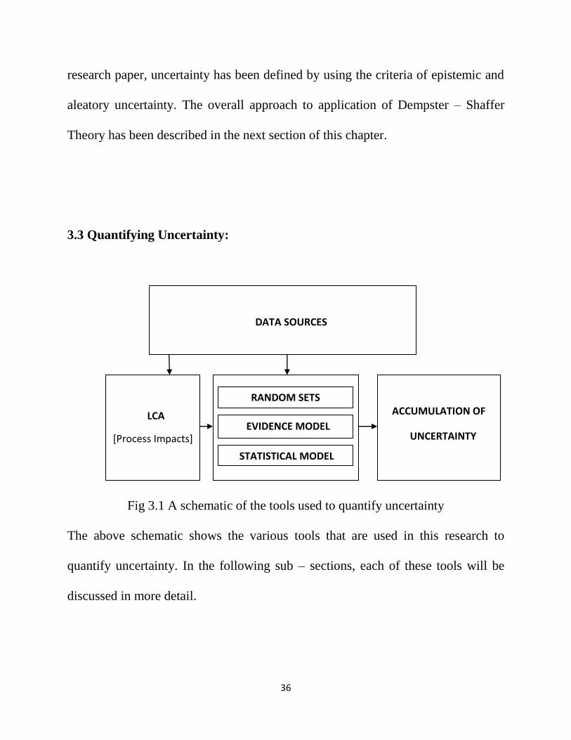
3.3 Quantifying Uncertainty:

Fig 3.1 A schematic of the tools used to quantify uncertainty

The above schematic shows the various tools that are used in this research to

quantify uncertainty. In the following sub – sections, each of these tools will be

discussed in more detail.

DATA SOURCES

LCA

[Process Impacts]

RANDOM SETS

EVIDENCE MODEL

STATISTICAL MODEL

ACCUMULATION OF

UNCERTAINTY

37

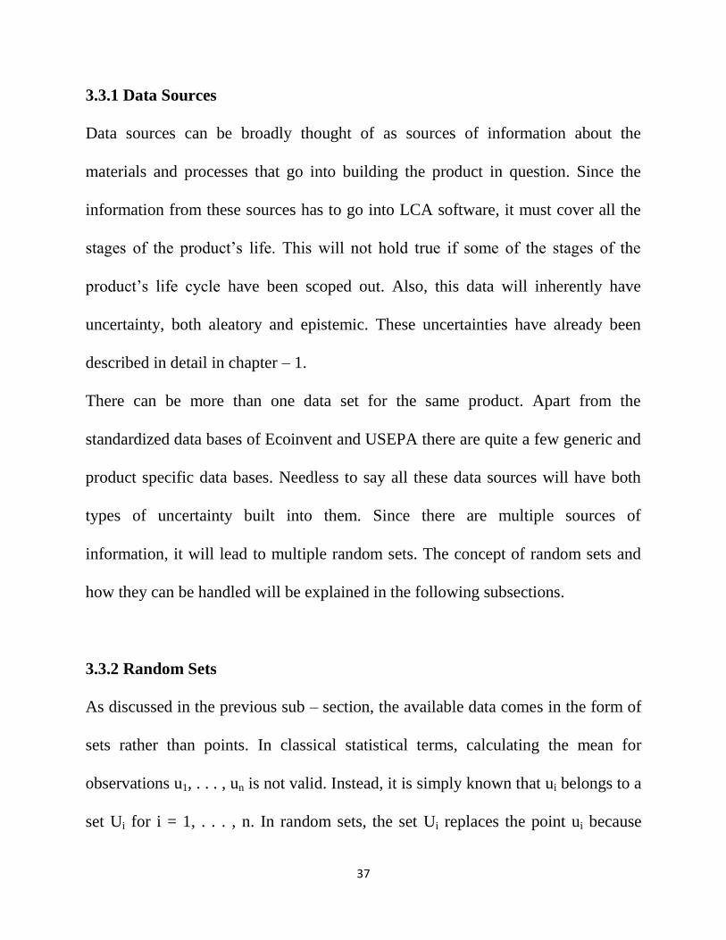
3.3.1 Data Sources

Data sources can be broadly thought of as sources of information about the

materials and processes that go into building the product in question. Since the

information from these sources has to go into LCA software, it must cover all the

stages of the product’s life. This will not hold true if some of the stages of the

product’s life cycle have been scoped out. Also, this data will inherently have

uncertainty, both aleatory and epistemic. These uncertainties have already been

described in detail in chapter – 1.

There can be more than one data set for the same product. Apart from the

standardized data bases of Ecoinvent and USEPA there are quite a few generic and

product specific data bases. Needless to say all these data sources will have both

types of uncertainty built into them. Since there are multiple sources of

information, it will lead to multiple random sets. The concept of random sets and

how they can be handled will be explained in the following subsections.

3.3.2 Random Sets

As discussed in the previous sub – section, the available data comes in the form of

sets rather than points. In classical statistical terms, calculating the mean for

observations u1, . . . , un is not valid. Instead, it is simply known that ui belongs to a

set Ui for i = 1, . . . , n. In random sets, the set Ui replaces the point ui because

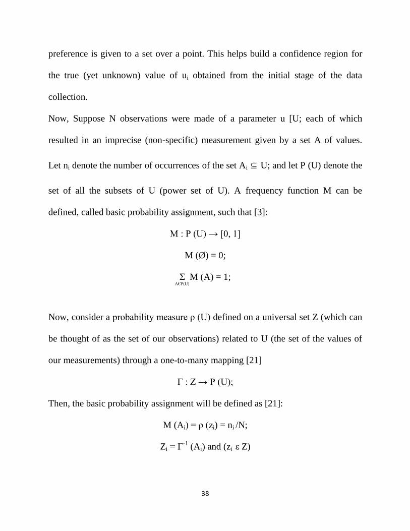
38

preference is given to a set over a point. This helps build a confidence region for

the true (yet unknown) value of ui obtained from the initial stage of the data

collection.

Now, Suppose N observations were made of a parameter u [U; each of which

resulted in an imprecise (non-specific) measurement given by a set A of values.

Let ni denote the number of occurrences of the set Ai ⊆ U; and let P (U) denote the

set of all the subsets of U (power set of U). A frequency function M can be

defined, called basic probability assignment, such that [3]:

M : P (U) → [0, 1]

M (Ø) = 0;

Σ M (A) = 1; AЄP(U)

Now, consider a probability measure ρ (U) defined on a universal set Z (which can

be thought of as the set of our observations) related to U (the set of the values of

our measurements) through a one-to-many mapping [21]

Γ : Z → P (U);

Then, the basic probability assignment will be defined as [21]:

M (Ai) = ρ (zi) = ni /N;

Zi = Γ-1

(Ai) and (zi ε Z)

39

3.3.3. Evidence Model

As stated initially, the classical probability theory cannot take the evidence into

account. But, since we want to take evidence into account, we will have to use the

Evidence Theory, also called Dempster – Shaffer theory. The significant

innovation of this framework is that it allows for the allocation of a probability

mass to sets or intervals. In traditional probability theory, evidence is associated

with only one possible event. In Dempster Shaffer Theory, evidence can be

associated with multiple possible events, e.g., sets of events. As a result, evidence

in DST can be meaningful at a higher level of abstraction without having to resort

to assumptions about the events within the evidential set [19]. Where the evidence

is sufficient enough to permit the assignment of probabilities to single events, the

Dempster-Shafer model collapses to the traditional probabilistic formulation. So, in

other words, the classical probability theory is a special case of the Dempster

Shafer Theory.

Since Dempster Shafer theory is a generalization of Bayesian Theory of subjective

probability, it is important to briefly explain Bayesian’s Theory. Bayesian Decision

Theory is a fundamental statistical approach that quantifies the tradeoffs between

various decisions using probabilities and costs that accompany such decisions. It is

based on Baye’s Rule [21]:

P (wi|x) = [P (x|wi) P (wi)] / P (x)

40

Bayesian interpretation of probability is a theorem to express how a subjective

degree of belief should rationally change to account for evidence. In other words,

Bayes' theorem then links the degree of belief in a proposition before and after

accounting for evidence. In this formula, P (wi) is the prior, i.e. the initial degree of

belief in A; P (wi|x), is the posterior i.e. the degree of belief, and the quotient

P(x|wi)/P(x) is the support B provides for A [23].

The basic probability assignment (bpa) is a primitive of evidence theory. Generally

speaking, the term “basic probability assignment” does not refer to probability in

the classical sense. The bpa, represented by m, defines a mapping of the power set

to the interval between 0 and 1, where the bpa of the null set is 0 and the

summation of the bpa’s of all the subsets of the power set is 1. The value of the bpa

for a given set A (represented as m(A)), expresses the proportion of all relevant and

available evidence that supports the claim that a particular element of X (the

universal set) belongs to the set A but to no particular subset of A. From the basic

probability assignment, the upper and lower bounds of an interval can be defined.

This interval contains the precise probability of a set of interest (in the classical

sense) and is bounded by two nonadditive continuous measures called Belief and

Plausibility. The lower bound Belief for a set A is defined as the sum of all the

basic probability assignments of the proper subsets (B) of the set of interest (A) (B Í

41

A). The upper bound, Plausibility, is the sum of all the basic probability

assignments of the sets (B) that intersect the set of interest (A) ().

Formally, for all sets A that are elements of the power set

Since Dempster Shafer theory is a generalization of Bayesian Theory of subjective

probability, it is important to briefly explain Bayesian’s Theory. Bayesian Decision

Theory is a fundamental statistical approach that quantifies the tradeoffs between

various decisions using probabilities and costs that accompany such decisions. It is

based on Baye’s Rule [21]:

P (wi|x) = [P (x|wi) P (wi)] / P (x)

Bayesian interpretation of probability is a theorem to express how a subjective

degree of belief should rationally change to account for evidence. In other words,

Bayes' theorem then links the degree of belief in a proposition before and after

accounting for evidence. In this formula, P (wi) is the prior, i.e. the initial degree of

belief in A; P (wi|x), is the posterior i.e. the degree of belief, and the quotient

P(x|wi)/P(x) is the support B provides for A [22].

Belief functions have been proposed for modeling someone’s degrees of belief.

They provide alternatives to the models based on probability functions or on

possibility functions. Dempster–Shafer theory covers several models that use the

42

mathematical object called ‘belief function’. Usually their aim is in the modeling of

someone’s degrees of belief, where a degree of belief is understood as a strength of

opinion. Beliefs result from uncertainty. Uncertainty sometimes results from a

random process (the objective probability case), it sometimes results only from the

lack of information that induces some ‘belief’ (‘belief’ must be contrasted to

‘knowledge’ as what is believed can be false) [23].

The next few paragraphs will describe the how belief function is quantified. We

start from a finite set of worlds which are called the “frame of discernment”.

Assume one of its words, ω0, corresponds to the actual world. An agent, denotes

You (it can correspond to a robot, a piece of software, or even something non-

tangible), does not know the world in which Ω corresponds to the actual world ω0.

So for every subset A of Ω, You can express the strength of Your opinion that the

actual world ω0 belongs to A. This strength is denoted belief(A), and belief means

(weighted) opinions. The larger the belief(A), the stronger You believe ω0 є A [23].

We suppose a finite propositional language L, supplemented by the tautology and

the contradiction. Let Ω denote the set of worlds that correspond to the

interpretations of L. It is built in such a way that no two worlds in Ω denote

logically equivalent propositions, i.e., for every pair of worlds in Ω, there exists a

43

proposition in the language L that is true in one world and false in the other.

Among the worlds in Ω, a particular one corresponds to the actual world ω0.

Because the data available to You are imperfect, You do not know exactly which

world in a set of possible worlds is the actual world ω0. All You can express is

Your ‘opinion’, represented by belief(A) for A ⊆ Ω, about the fact that the actual

world ω0 belongs to the various subsets A of Ω. The major problem is in the choice

of the properties that the function ‘belief’ should satisfy. We first assume that for

every pair of subsets A and B of Ω, belief(A) and belief(B) are comparable, i.e.,

belief(A) ≤ belief(B) or belief(A) ≥ belief(B) [24].

To simplify the above example, using basic probability assignment, the upper and

lower bounds of an interval can be defined. This interval contains the precise

probability of a set of interest (in the classical sense) and is bounded by two

nonadditive continuous measures called Belief and Plausibility. The lower bound

Belief for a set A is defined as the sum of all the basic probability assignments of

the proper subsets (B) of the set of interest (A) (B ⊆ A) [19]. The upper bound,

Plausibility, is the sum of all the basic probability assignments of the sets (B) that

intersect the set of interest Formally, for all sets A that are

elements of the power set [19]

44

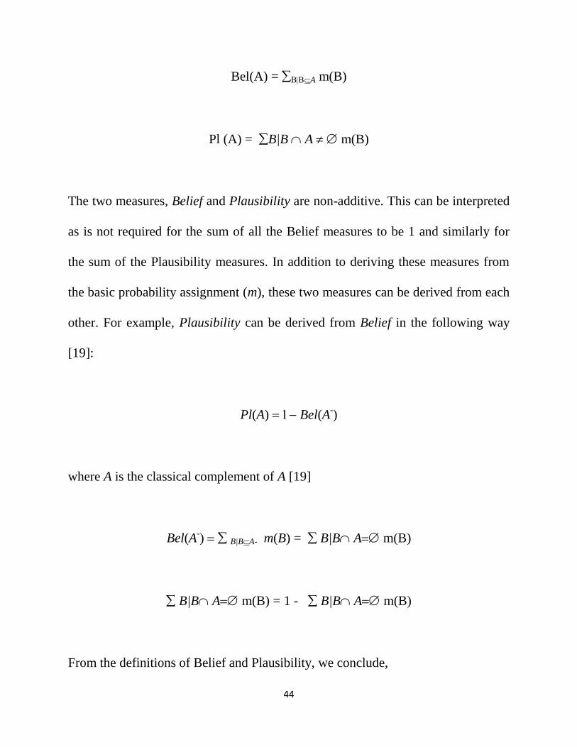
Bel(A) = A m(B)

Pl (A) = B|B A m(B)

The two measures, Belief and Plausibility are non-additive. This can be interpreted

as is not required for the sum of all the Belief measures to be 1 and similarly for

the sum of the Plausibility measures. In addition to deriving these measures from

the basic probability assignment (m), these two measures can be derived from each

other. For example, Plausibility can be derived from Belief in the following way

[19]:

Pl(A) Bel(A-)

where A is the classical complement of A [19]

Bel(A-) B|BA- m(B) =B|BAm(B)

B|BAm(B) = 1 - B|BAm(B)

From the definitions of Belief and Plausibility, we conclude,

45

Pl(A) = 1- Bel(A)

If one is given values of either (m(A) or Bel(A) or Pl(A)), it is possible to calculate

the values of the other two measures. The precise probability of an event (in the

classical sense) lies within the lower and upper bounds of Belief and Plausibility,

respectively.

Bel(A) = P(A) = Pl(A)

The probability is uniquely determined if Bel (A) = Pl(A). In this case, which

corresponds to classical probability, all the probabilities, P(A) are uniquely

determined for all subsets A of the universal set. Otherwise, Bel (A) and Pl(A) may

be viewed as lower and upper bounds on probabilities, respectively, where the

actual probability is contained in the interval described by the bounds. Upper and

lower probabilities derived by the other frameworks in generalized information

theory can not be directly interpreted as Belief and Plausibility functions [19].

3.3.4 Statistical Methods

Statistical Methods can only deal with aleatory uncertainty. They have already

been discussed in detail in Chapter – 2.

46

3.3.5 Aggregation of Uncertainty

The purpose of aggregation of information is to meaningfully summarize and

simplify a corpus of data whether the data is coming from a single source or

multiple sources. Familiar examples of aggregation techniques include arithmetic

averages, geometric averages, harmonic averages, maximum values, and minimum

values. Combination rules are the special types of aggregation methods for data

obtained from multiple sources. These multiple sources provide different

assessments for the same frame of discernment and Dempster-Shafer theory is

based on the assumption that these sources are independent. The requirement for

establishing the independence of sources is an important philosophical question.

There are multiple operators available in each category of pooling by which a

corpus of data can be combined. One means of comparison of combination rules is

by comparing the algebraic properties they satisfy. With the tradeoff type of

combination operations, less information is assumed than in a Bayesian approach

and the precision of the result may suffer as a consequence. On the other hand, a

precise answer obtained via the Bayesian approach does not express any

uncertainty associated with it and may have hidden assumptions of additivity or

Principle of Insufficient Reason. In keeping with this general notion of a

continuum of combination operations, there are multiple possible ways in which

47

evidence can be combined in Dempster Shaffer Theory, but in this case

Cumulative Distribution Function will be used [19].

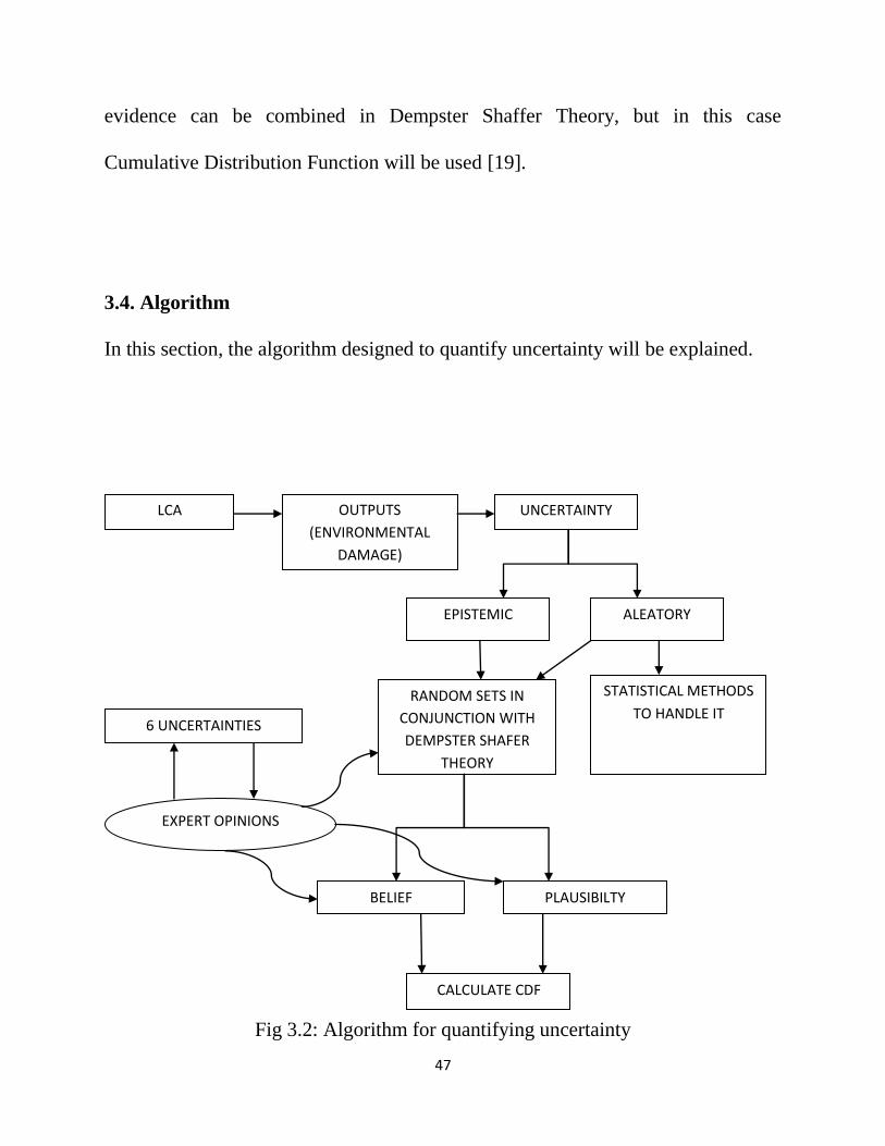
3.4. Algorithm

In this section, the algorithm designed to quantify uncertainty will be explained.

Fig 3.2: Algorithm for quantifying uncertainty

LCA OUTPUTS

(ENVIRONMENTAL

DAMAGE)

UNCERTAINTY

EPISTEMIC ALEATORY

6 UNCERTAINTIES

RANDOM SETS IN

CONJUNCTION WITH

DEMPSTER SHAFER

THEORY

STATISTICAL METHODS

TO HANDLE IT

EXPERT OPINIONS

BELIEF PLAUSIBILTY

CALCULATE CDF

48

3.4.1 LCA

A Life Cycle Analysis on the given product is done using the data available. The

analysis is done using the software SimaPro. Other commonly used software for

LCA is GaBi. The material quantity has to be input. For this particular research, a

TV remote control has been used. The data and disassembly techniques for the TV

remote control have been discussed in detail by Yang et al [25]. SimaPro has been

used for the LCA of this remote.

3.4.2 Outputs

The result of an LCA is environmental damage. Typically, LCA gives out how the

amount of harmful fluids and solids released into the atmosphere. Usually these

fluids and solids are measured by mass. Some examples of this might be carbon

dioxide, carcinogens, carbon monoxide and oxides of sulfur. In addition, the LCA

also gives out specific impacts caused by manufacturing that particular product.

These impacts are adverse impacts and the lesser their values, the more

environmentally benign the product is. Some examples of these impacts are global

warming, acidification, respiratory effects, eutrophication, ozone depletion, eco-

toxicity and smog. These impacts are categorized according to the stage of the

LCA in which they occurred. For example, the LCA software categorizes each of

49

the above mentioned impact types according to manufacturing stage, product

delivery stage, disposal delivery stage, end-of-life stage and use stage.

3.4.3 Uncertainty

It is known that there is some uncertainty in these results. It is so because the input

data used to calculate these results contains uncertainty. SimaPro does have an

option to quantify uncertainty using Monte Carlo analysis. Uncertainty is broadly

categorized as aleatory and epistemic. Both these types have been described in

detail in chapter – 1.

3.4.4 Random Sets in Conjunction with Dempster-Shafer Theory

The theory for random sets and D-S theory have been explained in detail in the

previous sections of this paper. Since, Yang et al provide single values for

environmental impacts, random sets have to be constructed.

3.4.5 Six Uncertainties and Expert Opinions

Aside from the broad categorization of uncertainty as epistemic and aleatory, many

researchers also believe that an uncertainty factor can rise due to the six following

reason: reliability, completeness, temporal correlation, geographic correlation,

technological considerations, sample size [26]. A rubric or a “pedigree matrix” can

then be constructed off of this knowledge. This helps in estimation of uncertainty.

50

The simplified approach includes a qualitative assessment of data quality

indicators based on a pedigree matrix. The pedigree matrix is based on “expert

opinions”. Each characteristic is divided into five quality levels with a score

between 1 and 5, based on this opinion. 1 refers to the most precise knowledge of

the characteristic in question and 5 refers to the least well known characteristic.

3.4.6 Belief and Plausibility

The theory for belief and plausibility functions has been described in the previous

sections of this paper. In this section we will discuss how it is relevant to this

algorithm. As has been defined, pedigree matrix is a means to express expert

opinion. It is this expert opinion that will influence the plausibility and belief

functions. The plausibility and belief functions will in turn impact how random sets

for this particular problem are defined.

3.4.7 Calculate CDF

CDF is the acronym for Cumulative Distribution Function. It is used to aggregate

the uncertainty.

51

3.4.8 Conclusion

In this chapter, an algorithm has been developed to quantify uncertainty. All of its

various elements have been explained in great detail. In addition its working has

also been discussed. In the next chapter, a demonstration of this theorem will be

given.

52

CHAPTER – 4

CALCULATIONS

In Chapter – 3, the methodology for quantification of uncertainty has been

discussed in great detail. This chapter will focus on a test case for the

demonstration of the methodology. As mentioned earlier, the inputs will be taken

from Yang et al [26] and the methodology has been inspired from Tonon [21]. The

concept of random sets and Dempster-Shaffer theory has already been discussed in

chapter – 3.

4.1 Input Data Sets

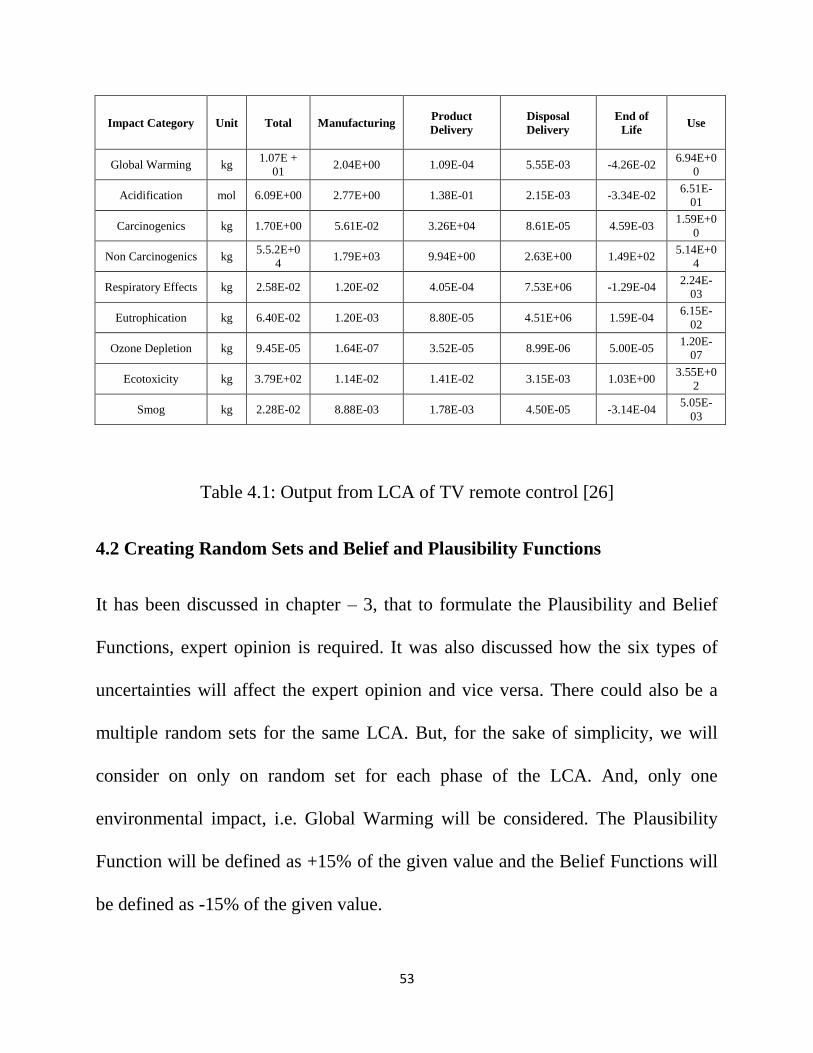
The input data is the environmental impacts obtained from LCA of TV remote

control [26]. The data is presented in a tabulated format in this section. The impact

categories considered here are Global Warming, Acidification, Carcinogenics, Non

Carcinogenics, Respiratory Effects, Eutrophication, Ozone Depletion, Ecotoxicity

and Smog. They are represented in the first column. The next columns contain the

contribution of each phase of the life cycle to these environmental impacts. The

phases in consideration here are: Manufacturing, Product Delivery, Disposal

Delivery and End of Life.

53

Impact Category Unit Total Manufacturing Product

Delivery

Disposal

Delivery

End of

Life Use

Global Warming kg 1.07E +

01 2.04E+00 1.09E-04 5.55E-03 -4.26E-02

6.94E+0

0

Acidification mol 6.09E+00 2.77E+00 1.38E-01 2.15E-03 -3.34E-02 6.51E-

01

Carcinogenics kg 1.70E+00 5.61E-02 3.26E+04 8.61E-05 4.59E-03 1.59E+0

0

Non Carcinogenics kg 5.5.2E+0

4 1.79E+03 9.94E+00 2.63E+00 1.49E+02

5.14E+0

4

Respiratory Effects kg 2.58E-02 1.20E-02 4.05E-04 7.53E+06 -1.29E-04 2.24E-

03

Eutrophication kg 6.40E-02 1.20E-03 8.80E-05 4.51E+06 1.59E-04 6.15E-

02

Ozone Depletion kg 9.45E-05 1.64E-07 3.52E-05 8.99E-06 5.00E-05 1.20E-

07

Ecotoxicity kg 3.79E+02 1.14E-02 1.41E-02 3.15E-03 1.03E+00 3.55E+0

2

Smog kg 2.28E-02 8.88E-03 1.78E-03 4.50E-05 -3.14E-04 5.05E-

03

Table 4.1: Output from LCA of TV remote control [26]

4.2 Creating Random Sets and Belief and Plausibility Functions

It has been discussed in chapter – 3, that to formulate the Plausibility and Belief

Functions, expert opinion is required. It was also discussed how the six types of

uncertainties will affect the expert opinion and vice versa. There could also be a

multiple random sets for the same LCA. But, for the sake of simplicity, we will

consider on only on random set for each phase of the LCA. And, only one

environmental impact, i.e. Global Warming will be considered. The Plausibility

Function will be defined as +15% of the given value and the Belief Functions will

be defined as -15% of the given value.

54

We know that

Bel(E) ≤ Pro(E) ≤ Pl(E) [2]

Where, Bel(E) is the Belief Function, Pro(E) is the Probability Function, and Pl(E)

is the Plausibility Function. Probability Function is defined by a Probability

Distribution Function (PDF).

The Random set is now discretized into intervals (Mfg min, Mfg mod) and (Mfg mod,

Mfg min) and into n1, and n2 subintervals Amfg, i = (ai, bi) respectively. Here Amfg, i is

the focal element. Also, p(mfg) is the PDF of Manufacturing phase and Fmfg (mfg)

is the Cumulative Distribution Function (CDF) for Manufacturing phase. The basic

probability assignment Mmfg(Amfg) is calculated for the focal element, Amfg,i, using

the following equations [21]:

Mmfg(Amfg) = ∫ Amfg,i p(m)dm = Fmfg (bi) - Fmfg (ai)

With the assigned numerical values, we get,

Mmfg(Amfg) = ½[(bi – 3.4680)*bi – (ai - 3.4680)*ai]

If Amfg,i є [Mfg min, Mfg mod]

And, Mmfg(Amfg) = ½[(- bi + 4.6920)]* bi + (ai - 4.6920)]* ai]

55

If Amfg,i є (Mfg mod, Mfg min)

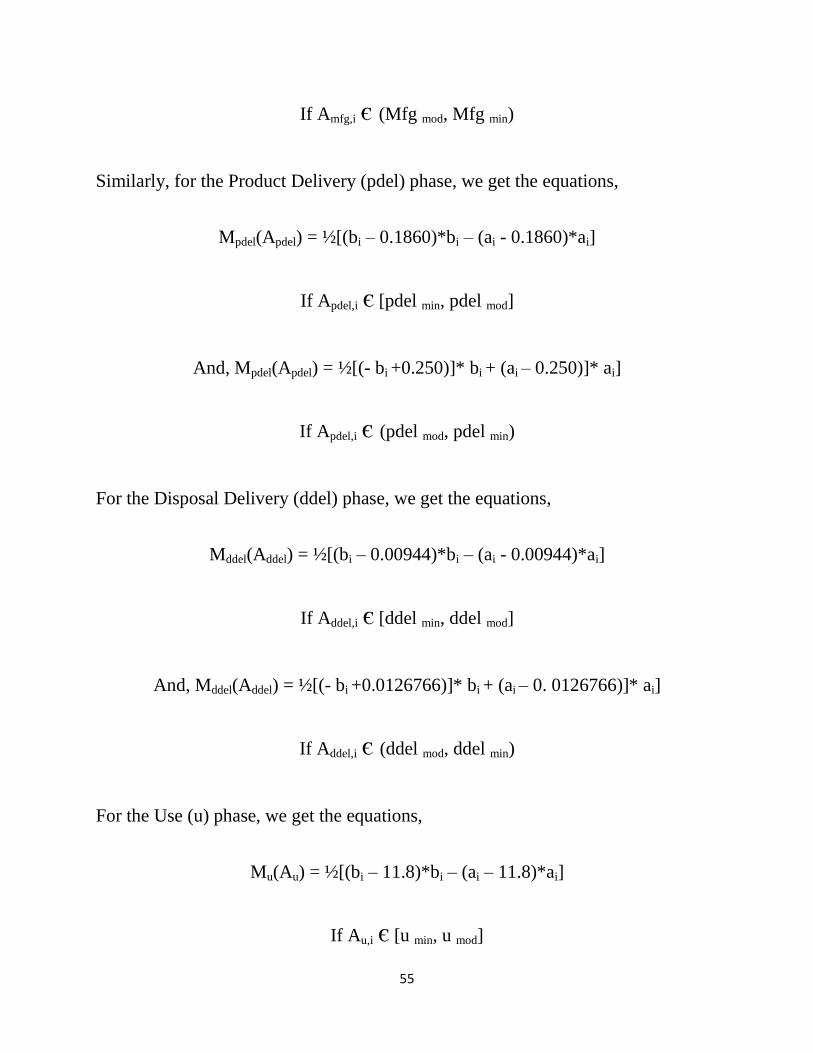
Similarly, for the Product Delivery (pdel) phase, we get the equations,

Mpdel(Apdel) = ½[(bi – 0.1860)*bi – (ai - 0.1860)*ai]

If Apdel,i є [pdel min, pdel mod]

And, Mpdel(Apdel) = ½[(- bi +0.250)]* bi + (ai – 0.250)]* ai]

If Apdel,i є (pdel mod, pdel min)

For the Disposal Delivery (ddel) phase, we get the equations,

Mddel(Addel) = ½[(bi – 0.00944)*bi – (ai - 0.00944)*ai]

If Addel,i є [ddel min, ddel mod]

And, Mddel(Addel) = ½[(- bi +0.0126766)]* bi + (ai – 0. 0126766)]* ai]

If Addel,i є (ddel mod, ddel min)

For the Use (u) phase, we get the equations,

Mu(Au) = ½[(bi – 11.8)*bi – (ai – 11.8)*ai]

If Au,i є [u min, u mod]

56

And, Mu(Au) = ½[(- bi + 15.96)]* bi + (ai – 15.96)]* ai]

If Au,i є (u mod, u min)

Once, the random sets are discretized, the respective Cumulative Distribution

Functions are calculated. These Cumulative Distribution functions give an

aggregation of probability. The calculation is done by summing up the weights

(Basic Probability Assignment) i.e. Mmfg(Ai) etc separately for each phase. The

calculations for discretization of random sets and the corresponding CDFs have

been shown in the following subsections.

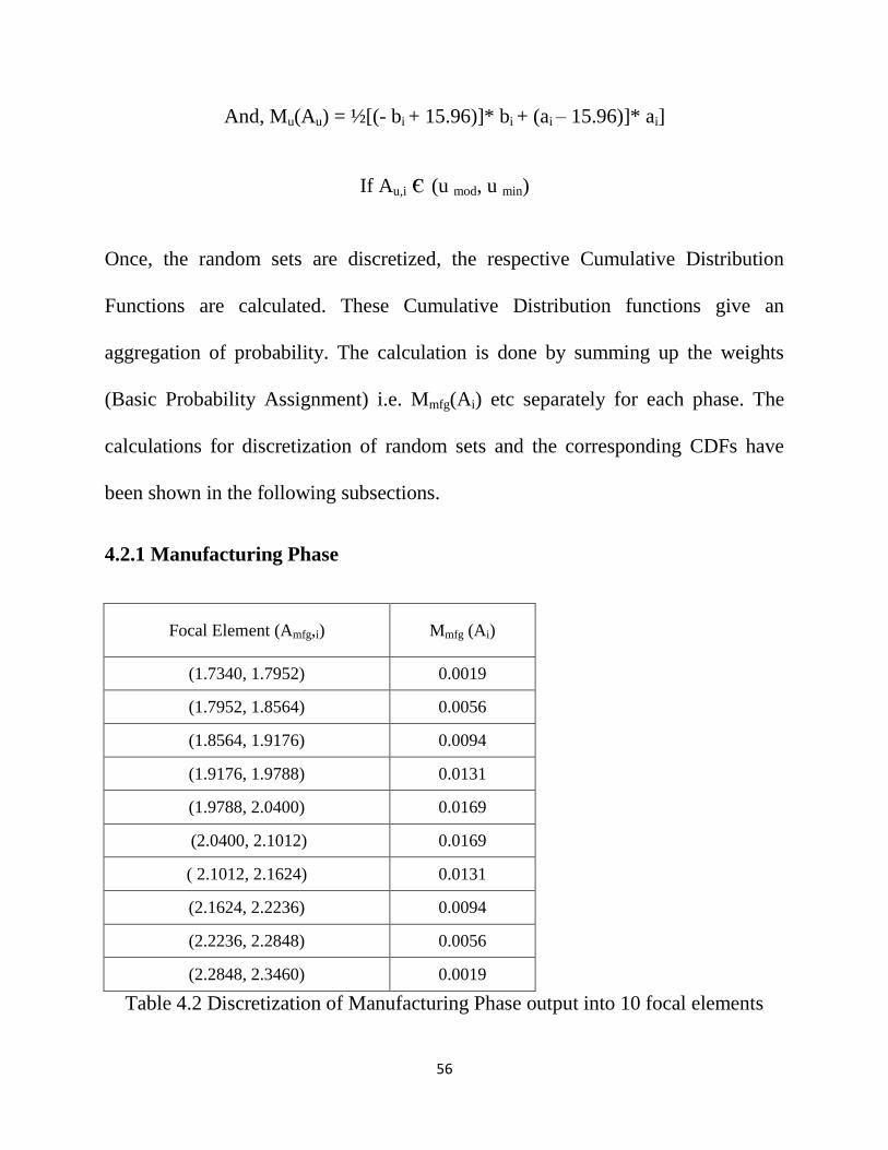
4.2.1 Manufacturing Phase

Focal Element (Amfg,i) Mmfg (Ai)

(1.7340, 1.7952) 0.0019

(1.7952, 1.8564) 0.0056

(1.8564, 1.9176) 0.0094

(1.9176, 1.9788) 0.0131

(1.9788, 2.0400) 0.0169

(2.0400, 2.1012) 0.0169

( 2.1012, 2.1624) 0.0131

(2.1624, 2.2236) 0.0094

(2.2236, 2.2848) 0.0056

(2.2848, 2.3460) 0.0019

Table 4.2 Discretization of Manufacturing Phase output into 10 focal elements

57

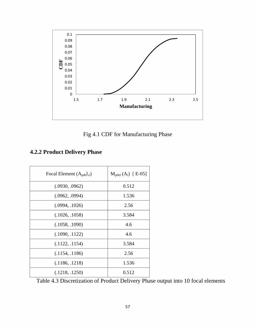
Fig 4.1 CDF for Manufacturing Phase

4.2.2 Product Delivery Phase

Focal Element (Apdel,i) Mpdel (Ai) [ E-05]

(.0930, .0962) 0.512

(.0962, .0994) 1.536

(.0994, .1026) 2.56

(.1026, .1058) 3.584

(.1058, .1090) 4.6

(.1090, .1122) 4.6

(.1122, .1154) 3.584

(.1154, .1186) 2.56

(.1186, .1218) 1.536

(.1218, .1250) 0.512

Table 4.3 Discretization of Product Delivery Phase output into 10 focal elements

0

0.01

0.02

0.03

0.04

0.05

0.06

0.07

0.08

0.09

0.1

1.5 1.7 1.9 2.1 2.3 2.5

CD

F

Manufacturing

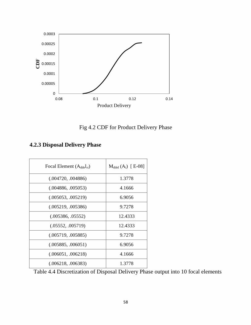
58

Fig 4.2 CDF for Product Delivery Phase

4.2.3 Disposal Delivery Phase

Focal Element (Addel,i) Mddel (Ai) [ E-08]

(.004720, .004886) 1.3778

(.004886, .005053) 4.1666

(.005053, .005219) 6.9056

(.005219, .005386) 9.7278

(.005386, .05552) 12.4333

(.05552, .005719) 12.4333

(.005719, .005885) 9.7278

(.005885, .006051) 6.9056

(.006051, .006218) 4.1666

(.006218, .006383) 1.3778

Table 4.4 Discretization of Disposal Delivery Phase output into 10 focal elements

0

0.00005

0.0001

0.00015

0.0002

0.00025

0.0003

0.08 0.1 0.12 0.14

CD

F

Product Delivery

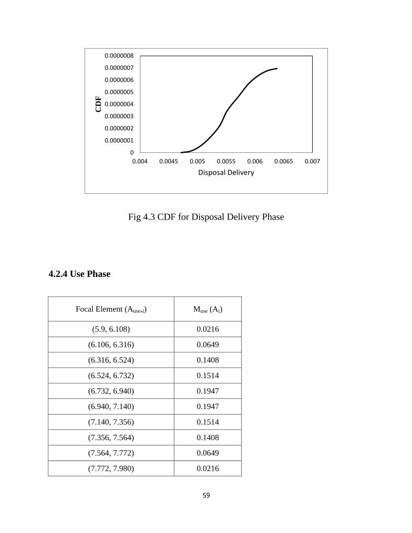
59

Fig 4.3 CDF for Disposal Delivery Phase

4.2.4 Use Phase

Focal Element (Ause,i) Muse (Ai)

(5.9, 6.108) 0.0216

(6.106, 6.316) 0.0649

(6.316, 6.524) 0.1408

(6.524, 6.732) 0.1514

(6.732, 6.940) 0.1947

(6.940, 7.140) 0.1947

(7.140, 7.356) 0.1514

(7.356, 7.564) 0.1408

(7.564, 7.772) 0.0649

(7.772, 7.980) 0.0216

0

0.0000001

0.0000002

0.0000003

0.0000004

0.0000005

0.0000006

0.0000007

0.0000008

0.004 0.0045 0.005 0.0055 0.006 0.0065 0.007

CD

F

Disposal Delivery

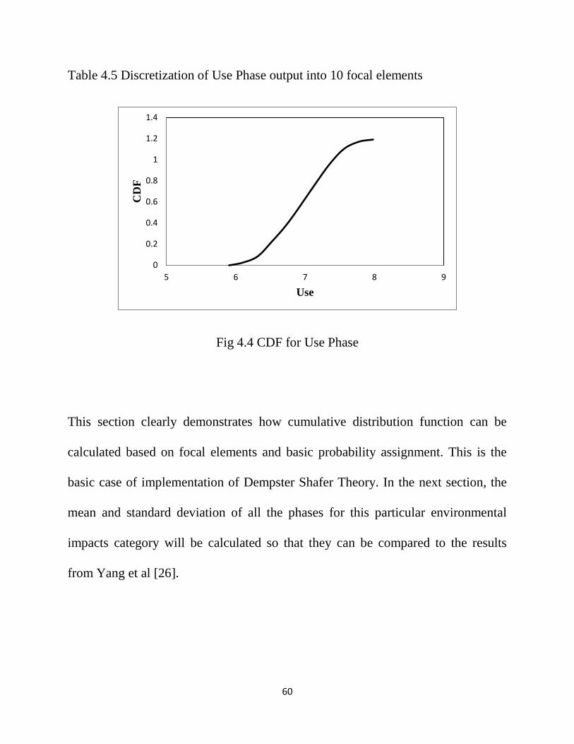
60

Table 4.5 Discretization of Use Phase output into 10 focal elements

Fig 4.4 CDF for Use Phase

This section clearly demonstrates how cumulative distribution function can be

calculated based on focal elements and basic probability assignment. This is the

basic case of implementation of Dempster Shafer Theory. In the next section, the

mean and standard deviation of all the phases for this particular environmental

impacts category will be calculated so that they can be compared to the results

from Yang et al [26].

0

0.2

0.4

0.6

0.8

1

1.2

1.4

5 6 7 8 9

CD

F

Use

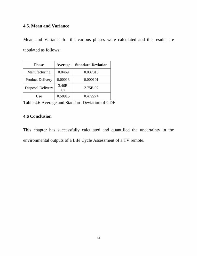
61

4.5. Mean and Variance

Mean and Variance for the various phases were calculated and the results are

tabulated as follows:

Phase Average Standard Deviation

Manufacturing 0.0469 0.037316

Product Delivery 0.00013 0.000101

Disposal Delivery 3.46E-

07 2.75E-07

Use 0.58915 0.472274

Table 4.6 Average and Standard Deviation of CDF

4.6 Conclusion

This chapter has successfully calculated and quantified the uncertainty in the

environmental outputs of a Life Cycle Assessment of a TV remote.

62

CHAPTER - 5

CONTRIBUTIONS AND FUTURE WORK

This study was set out to explore various existing techniques to quantify

uncertainty in Life Cycle Analysis (LCA). Quantifying uncertainty in LCA is

necessary to ensure that designers obtain meaningful information on the reliability

of results from LCA. The contributions of this thesis are highlighted below

followed by future work.

5.1 Contributions

This research has successfully

Developed a model utilizing evidence theory and random sets to incorporate

epistemic uncertainty in Life cycle analysis.

Combined epistemic and aleatory uncertainty by utilizing Dempster Shafer

Theory with distributions on random sets in the model.

Incorporated the use of 6 types of epistemic uncertainty highlighted in the

literature.

Developed an algorithm and implemented in Matlab based on the proposed

model.

63

Demonstrated the application of the algorithm and the proposed model

through a preliminary example of LCA study and uncertainty analysis of a

TV remote.

Although, there are many environmental impact categories which form the output

of any LCA, for the purpose of this study the impact category of Global Warming

was considered. The study found that the uncertainty values calculated using

Dempster Shafer Theory are more realistic, unlike the results calculated using

Monte Carlo Analysis which is built in SimaPro. The reason for this is that

Dempster Shafer Theory inherently takes into account the evidence for the degree

of accuracy of the data. The study has also successfully proved that uncertainty in

LCA can be quantified by calculating it in conjunction with Dempster Shafer

Theory.

5.2 Future work

It is also the author’s belief that there are also some areas where this model needs

expansion and more work. A few improvements that can be made are

Utilizing a rubric for generating belief and plausibility functions based on 6

sources of uncertainty in LCA data

64

Demonstrating the model for each process in LCA rather than stage of life

cycle

Comparing the computational complexity of the proposed model with

monte-carlo simulations.

Exploring combinations of epistemic and aleatory uncertainty that has

correlated environmental impacts when statistical information (aleatory

portion) is available.

65

References:

1.) Life Cycle Assessment: Principles and Practice; 2006, U.S. Environmental

Protection Agency

2.) Lloyd, S. M., & Ries, R. (2007). Characterizing, Propagating, and Analyzing

Uncertainty in Life‐Cycle Assessment: A Survey of Quantitative Approaches.

Journal of Industrial Ecology, 11(1), 161-179.

3.) Schlosser, J., & Paredis, C. J. (2007, April). Managing multiple sources of

epistemic uncertainty in engineering decision making. In Proceedings of the

society of automotive engineering world congress, Detroit, MI (pp. 16-19).

4.) Baker, J. W., & Lepech, M. D. (2009, September). Treatment of uncertainties

in life cycle assessment. In Intl. Congress on Structral Safety and Reliability.

5.) EPA Website http://www.epa.gov/

6.) Huijbregts, Mark Antonius Jan, “Uncertainty and variability in

environmental life – cycle assessment”, Academic Proefschrift – 2001

7.) Björklund, A.E. Survey of Approaches to Improve Reliability in LCA.

International Journal of Life Cycle Assessment 7: 2 (2002), 64-72.

8.) Huijbregts, Mark A., Norris, Gregory, Bretz, Rolf, Ciroth Andreas, Maurice,

Benoit, Bahr, Bo von, Weidema, Bo, “Framework for Modeling Data Uncertainty

66

in Life Cycle Inventories” The International Journal of Life Cycle Assessment.May

2001, Volume 6, Issue 3, pp 127-132

9.) Baker, Jack W., Lepech, Michael D. “Treatment of Uncertainties in

Life Cycle Assessment” Stanford University, Stanford, USA, 2009

10.) Heijungs, Reinout, Frischknecht, Rolf, “Representing Statistical Distributions

for Uncertain Parameters in LCA: Relationships between mathematical forms,

their representations in Ecospold, and heir representations in CMLCA”

International Journal of Life Cycle Assessment May 2005, Volume 10, Issue 4, pp

248-254

11.) Roos, Elin, Sandberg, Cecilla, Hansson, Per-Anders, “Uncertainties in

the carbon footprint of food products : a case study on table potatoes”

Emerald Group Publishing Limited, 2011

12.) Schlosser, J., & Paredis, C. J. (2007, April). Managing multiple sources of

epistemic uncertainty in engineering decision making. In Proceedings of the

society of automotive engineering world congress, Detroit, MI (pp. 16-19).

13.) Costello, A., Abbas, M., Allen, A., Ball, S., Bell, S., Bellamy, R., ... &

Patterson, C. (2009). Managing the health effects of climate change: lancet and

University College London Institute for Global Health Commission. The Lancet,

373(9676), 1693-1733.

67

14.) Ciroth, A., Fleischer, G., & Steinbach, J. (2004). Uncertainty calculation in

life cycle assessments. The International Journal of Life Cycle Assessment, 9(4),

216-226.

15.) Williams, E. D., Weber, C. L., & Hawkins, T. R. (2009). Hybrid framework

for managing uncertainty in life cycle inventories. Journal of Industrial Ecology,

13(6), 928-944.

16.) Hong, J., Shaked, S., Rosenbaum, R. K., & Jolliet, O. (2010). Analytical

uncertainty propagation in life cycle inventory and impact assessment: application

to an automobile front panel. The International Journal of Life Cycle Assessment,

15(5), 499-510.

17.) Segalman, D. J., Brake, M. R., Bergman, L. A., Vakakis, A., & Willner, K.

(2013). Epistemic and Aleatoric Uncertainty in Modeling (No. SAND2013-

0674C). Sandia National Laboratories.

18.) Behdad, S., Joseph, A. T., & Thurston, D. (2013, August). Systems Simulation

of Design for End-of-Life Recovery Under Uncertainty. In ASME 2013

International Design Engineering Technical Conferences and Computers and

Information in Engineering Conference (pp. V004T05A029-V004T05A029).

American Society of Mechanical Engineers.

68

19.) Sentz, Karl and Ferson, Scott “Combination of Evidence in Dempster Shafer

Theory” (2002) Sandia Report SAND2002-0835

20.) Zadeh, Lotfi A., (1995) “Discussion: Probability Theory and Fuzzy Logic are

Complimentary Rather Than Competitive” Technometrics, August 1995, Vol. 37,

No. 3

21.) Tonon, Fulvio, (2004) “Using random set theory to propagate epistemic

uncertainty through a mechanical system” Reliability Engineering and System

Safety 85 (2004) 169–181

23.) Berger, J. (1985), Statistical Decision Theory and Bayesian Analysis.

24.) Smets, P., "Belief Functions and the Transferable Belief Model." Available at

http://ippserv.rug.ac.be. The Imprecise Probabilities Project.

25.) Shafer, G., & Logan, R. (1987). Implementing Dempster's rule for hierarchical

evidence. Artificial Intelligence, 33(3), 271-298.

26.) Hu, Y., & Ameta, G. (2013, August). Life Cycle Assessment and Eco-Design

of a Wireless TV/VCR Remote. In ASME 2013 International Design Engineering

Technical Conferences and Computers and Information in Engineering

Conference (pp. V02AT02A049-V02AT02A049). American Society of

Mechanical Engineers.

69

27.) Frischknecht, R., Jungbluth, N., Althaus, H. J., Doka, G., Heck, T., Hellweg,

S., & Wernet, G. (2007). Overview and methodology. Ecoinvent Rep, 1, 237.