Embed Size (px)
Citation preview
AN ANALYZING MODEL OF STRESS-RELATED WELLBORE STRENGTHENING
TECHNIQUES
A Thesis
by
HUSSAIN IBRAHIM H ALBAHRANI
Submitted to the Office of Graduate and Professional Studies of
Texas AampM University
in partial fulfillment of the requirements for the degree of
MASTER OF SCIENCE
Chair of Committee Samuel F Noynaert
Committee Members Jerome J Schubert
Marcelo Sanchez
Head of Department A Daniel Hill
August 2015
Major Subject Petroleum Engineering
Copyright 2015 Hussain Ibrahim H AlBahrani
ii
ABSTRACT
One of the major causes of nonproductive time (NPT) and the resulting
additional costs during drilling operations is lost circulation The problem of lost
circulation is an ever growing concern to the operators for several reasons including the
continuous depletion of reservoirs and the naturally occurring narrow drilling window
due to an abnormally pressured interval or simply the low fracture pressure gradient of
the formation rock To deal with the issue of lost circulation the concept of wellbore
strengthening was introduced The ultimate goal of this concept is to increase the drilling
fluid pressure required to fracture the formation thus eliminating lost circulation and
NPT and reducing the costs Numerous wellbore strengthening techniques were created
for this purpose over the years Those techniques vary in their applicability to different
scenarios and their effectiveness Therefore there is a clear need for a tool that will help
to define the most suitable wellbore strengthening technique for a well-defined scenario
The model described in this study aims to provide a practical tool that evaluates
and predicts the performance of wellbore strengthening techniques in practical
situations The wellbore strengthening techniques covered by the model use stress
changes around the wellbore as the primary criteria for enhancing the fracture pressure
and effectively enlarging the drilling window The model uses geometric principles
basic rock mechanics data linear elasticity plane stress theory drilling fluid data and
geological data to evaluate and predict the performance of a wellbore strengthening
iii
technique Another important objective of the model is the proper selection of candidates
for wellbore strengthening To achieve that goal the model creates all of the possible
scenarios in terms of well placement surface location and trajectory based on the input
data to emphasize the scenario that will yield maximum results using a specific wellbore
strengthening technique
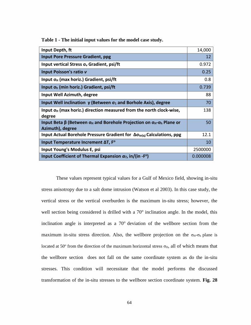
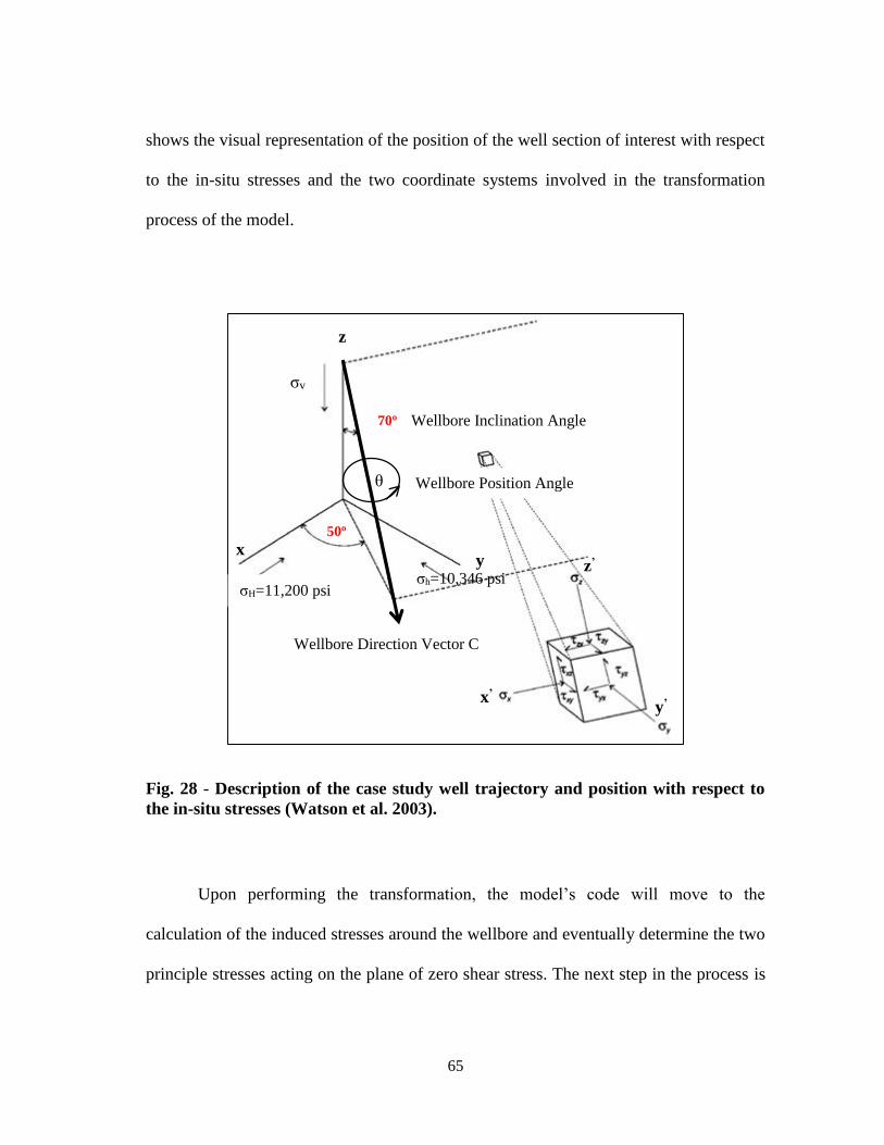
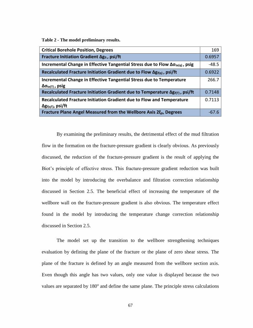
The use of the model is illustrated through the use of a case study The results of
the case study show practical advantages of applying the model in the well planning
phase The analysis performed using the model will demonstrate the applicability of a
certain wellbore strengthening technique the effectiveness of the technique and the best
parameters for the technique Therefore the analysis shows not only the best case
scenario for applying a wellbore strengthening technique but it also illustrates the cases
where applying the technique should be avoided due to an expected unsatisfactory
performance
iv
DEDICATIONS
I would like to dedicate this work to my family especially my father for passing
his work ethics on to me and my mother for all her devotion and sacrifice I would also
like to dedicate this work to my fianceacutee Sara who remained patient and supportive of
this endeavor from overseas for two long years
v
ACKNOWLEDGEMENTS
I would like to acknowledge the following for their invaluable contributions to
the process of completing this work and for supporting me throughout this undertaking
I would first like to acknowledge my committee chair Dr Samuel F Noynaert
for his support guidance and most importantly for providing me with the best possible
environment to do this work I would also like to thank my committee members Dr
Jerome J Schubert and Dr Marcelo Sanchez for being the source for many of the ideas
used to accomplish this work through their taught courses and for their time and effort
spent in making sure this research is accurate
I would also like to express my deep appreciation for Mr Fred Dupriest for
inspiring me the main idea of this research and for his instrumental contributions that
followed
I would be remiss if I did not acknowledge my sponsor and my employers Saudi
Aramco especially my supervisor Mr Nasser Khanferi for believing in me and giving
me this tremendous opportunity to expand my knowledge and improve my skills as a
researcher
Finally my sincere and everlasting gratitude for all the help I received from all
the faculty students and staff in the Texas AampM University Petroleum Engineering
Department especially my great friend Zuhair Al-yousef
vi
TABLE OF CONTENTS
Page
ABSTRACT ii
DEDICATIONS iv
ACKNOWLEDGEMENTS v
TABLE OF CONTENTS vi
LIST OF FIGURES viii
LIST OF TABLES xiii
11 INTRODUCTION 1
11 Wellbore Strengthening Definition 1 12 Objectives 4
22 MODEL DESCRIPTION 6
21 Model Introduction 6 22 In-Situ Stress Transformation 7
221 In-Situ Stress Description 7 222 The Transformation to the Wellbore Coordinates 11
23 Induced Borehole Stresses 16 24 Plane Stress Transformation 20 25 Model Assumptions and the Corresponding Implications and Corrections 31 26 The Evaluation of Fracture-Pressure Gradient Enhancement 41
261 Evaluation of Wellbore Strengthening Techniques from Basic Rock Mechanics 44
27 Model Interface 52
33 MODEL RESULTS AND ANALYSIS (CASE STUDY SCENARIO) 63
31 The Case Study Setup 63 32 The Preliminary Results 66 33 Wellbore Strengthening Evaluation Data and Preliminary Results 68 34 Parametric Analysis 70
341 First Stage Parametric Analysis 72
vii
3411 First stage Poissonrsquos ratio analysis 73 3412 First stage Youngrsquos modulus analysis 75 3413 First stage wellbore azimuth analysis 78 3414 First stage wellbore inclination analysis 79
342 Second Stage Parametric Analysis 83 3421 Second stage Poissonrsquos ratio analysis 83 3422 Second stage Youngrsquos modulus analysis 87 3423 Second stage wellbore inclination analysis 89 3424 Second stage wellbore diameter analysis 92 3425 Second stage fracture aperture analysis 94 3426 Second stage fracture toughness analysis 97 3427 Second stage fracture plug placement analysis 99 3428 Second stage fracture-pressure buildup analysis 101
343 Well Placement Evaluation 104
44 CONCLUSIONS 118
NOMENCLATURE 120
REFERENCES 126
viii
LIST OF FIGURES
Page
Fig 1 - A general illustration of a drilling window (Mitchell et al 2011) 2
Fig 2 - The world in-situ stress map showing direction and magnitude of stresses
(Tingay et al 2006) 8
Fig 3 - The pattern of borehole breakout and induced fractures on reference to the
direction of the earth in-situ stresses direction (Dupreist et al 2008) 9
Fig 4 - The estimation of the maximum horizontal stress based on the shape of the
borehole (Duffadar et al 2013) 10
Fig 5 - The relationship between the in-situ stresses reference frame and the defined
wellbore section reference frame (Watson et al 2003) 12
Fig 6 - The concentration of stress due to the presence of a wellbore 16
Fig 7 - The illustration of the resulting induced stress acting on an element of the
wellbore (Amadei et al 1997b) 20
Fig 8 - The contrast between determining the direction of the fracture in a vertical
section and in a horizontal section 22
Fig 9 - The relationship between the induced stresses reference frame and the plane
stresses reference frame 24
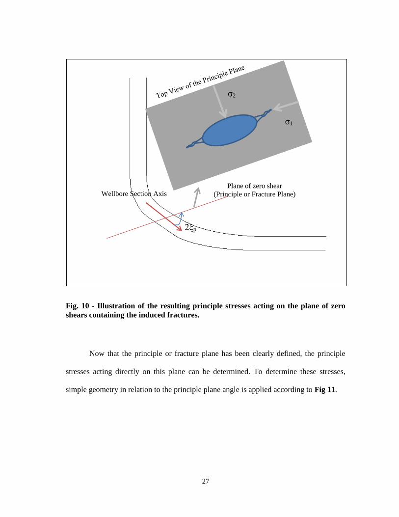
Fig 10 - Illustration of the resulting principle stresses acting on the plane of zero
shears containing the induced fractures 27
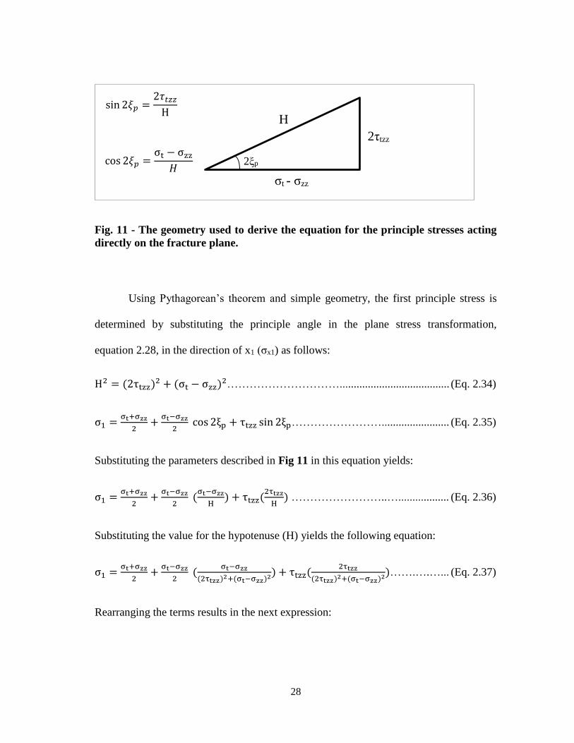
Fig 11 - The geometry used to derive the equation for the principle stresses acting
directly on the fracture plane 28
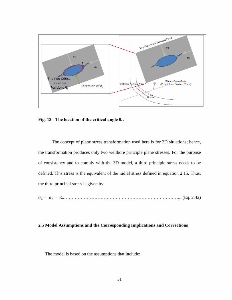
Fig 12 - The location of the critical angle θc 31
Fig 13 - The effect of in-situ earth stress field on the shape of the borehole (Duffadar
et al 2013) 34
ix
Fig 14 - The local change to the pore pressure due to mud filtration (Watson et al
2003) 35
Fig 15 - Illustration of the change undergone by the effective hoop stress as a result
of wellbore wall flow due to overbalance 37
Fig 16 - Illustration of the effect of the buildup of filter-cake as a drop in pressure
from the wellbore to the sand face due to its impermeable nature 38
Fig 17 -The contrast between the bottomhole formation and bottomhole fluid
temperatures and the temperature of the drilling fluid (Raymond 1969) 39
Fig 18 - The resulting narrower drilling window due to reservoir depletion 42
Fig 19 - The three mode of fracture loadings or openings according to fracture
mechanics (Jaeger et al 2007) 45
Fig 20 - The description of the sealed fracture scenario of particle and fracture
interaction in wellbore strengthening (Morita et al 2012) 47
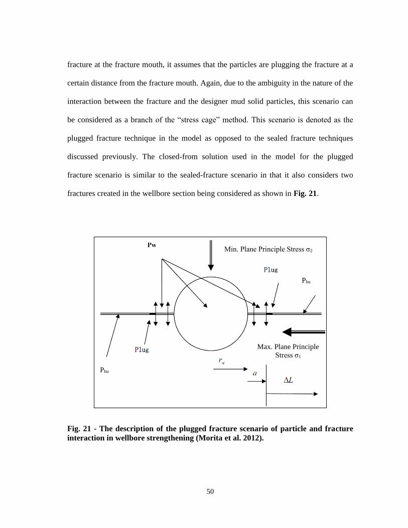
Fig 21 - The description of the plugged fracture scenario of particle and fracture
interaction in wellbore strengthening (Morita et al 2012) 50
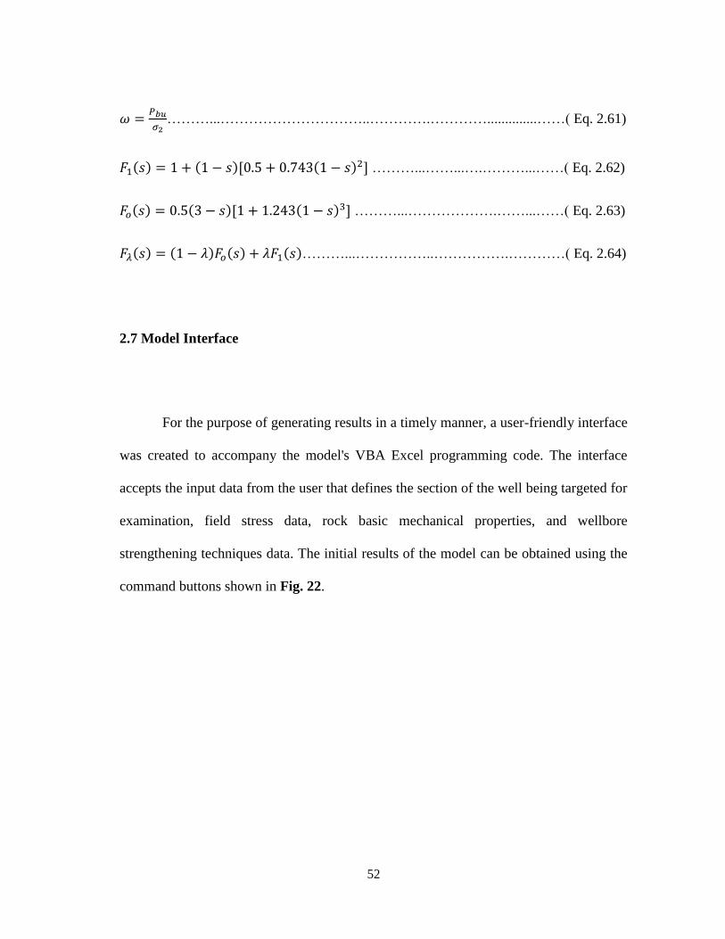
Fig 22 - The command buttons used in the model to obtain the initial results 53
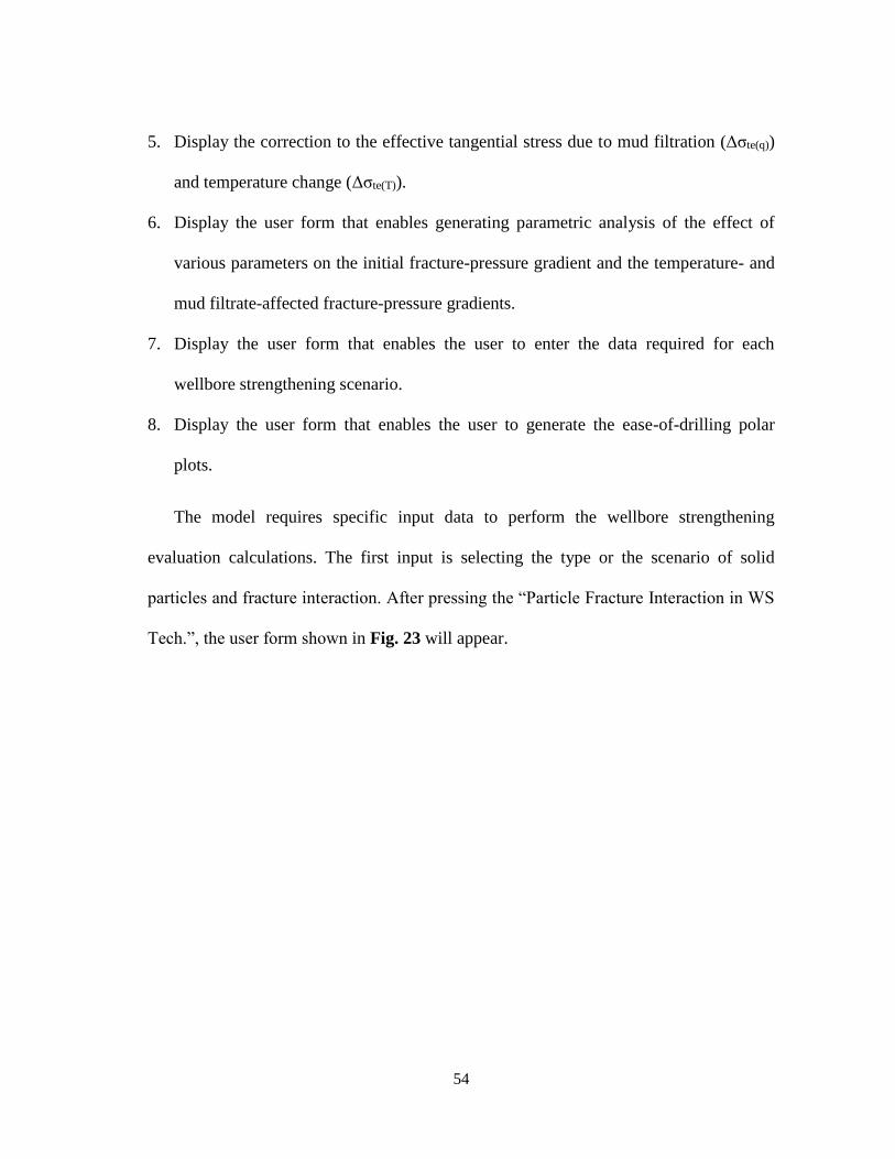
Fig 23 - The user form that enables the model to select the particle and fracture
interaction scenario and input the data for each scenario 55
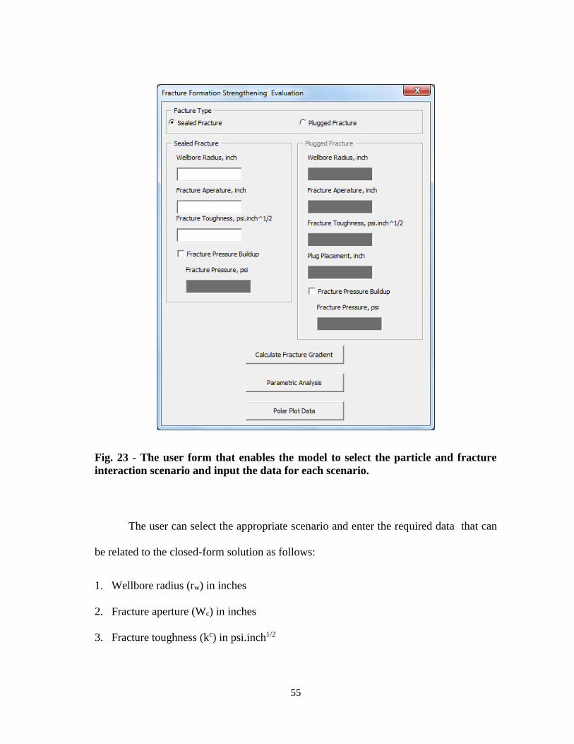
Fig 24 - The user form that enables selecting the base variable for the initial
parametric analysis 56
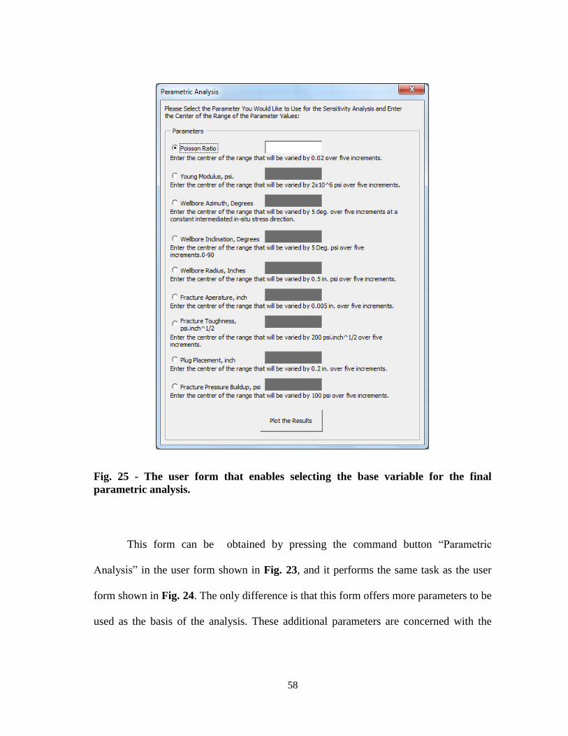
Fig 25 - The user form that enables selecting the base variable for the final
parametric analysis 58
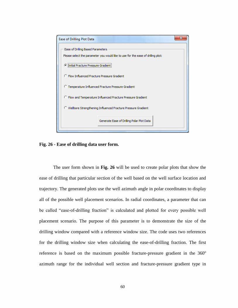
Fig 26 - Ease of drilling data user form 60
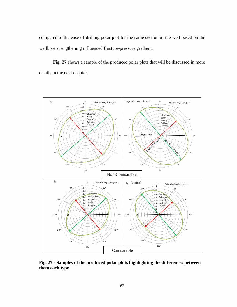
Fig 27 - Samples of the produced polar plots highlighting the differences between
them each type 62
Fig 28 - Description of the case study well trajectory and position with respect to the
in-situ stresses (Watson et al 2003) 65
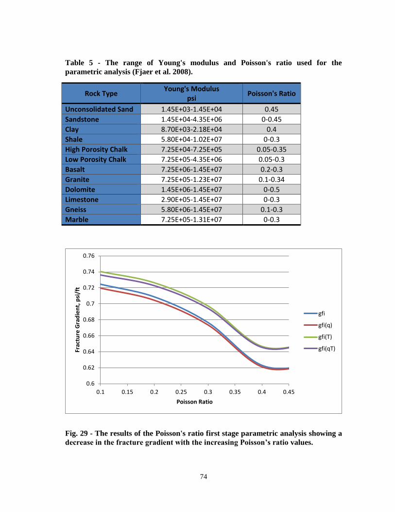
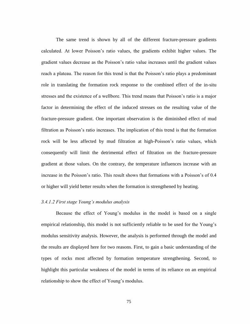
Fig 29 - The results of the Poissons ratio first stage parametric analysis showing a
decrease in the fracture gradient with the increasing Poissonrsquos ratio values 74
x
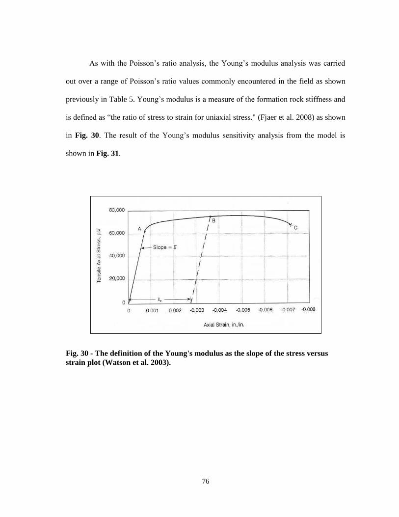
Fig 30 - The definition of the Youngs modulus as the slope of the stress versus strain
plot (Watson et al 2003) 76
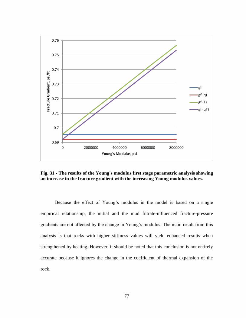
Fig 31 - The results of the Youngs modulus first stage parametric analysis showing
an increase in the fracture gradient with the increasing Young modulus values 77
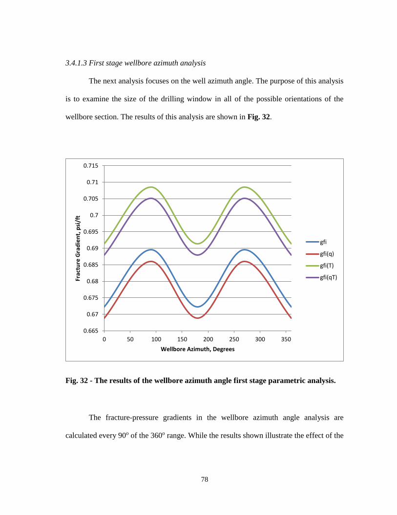
Fig 32 - The results of the wellbore azimuth angle first stage parametric analysis 78
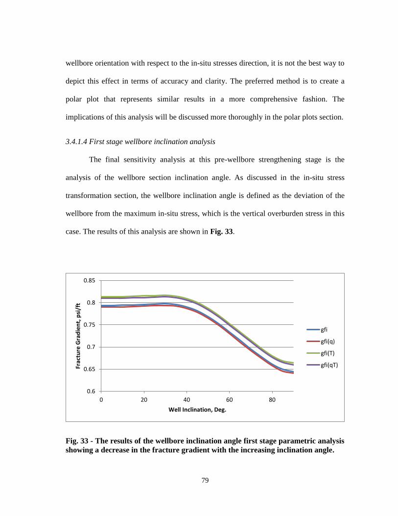
Fig 33 - The results of the wellbore inclination angle first stage parametric analysis
showing a decrease in the fracture gradient with the increasing inclination
angle 79
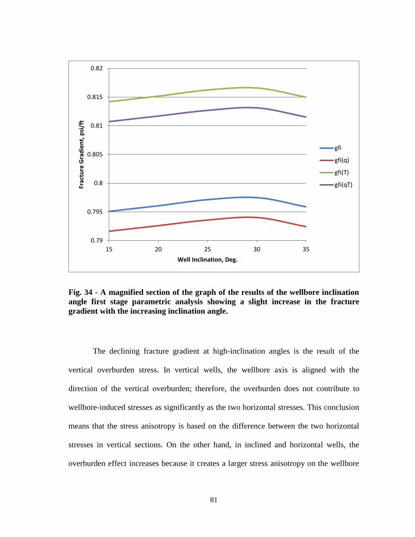
Fig 34 - A magnified section of the graph of the results of the wellbore inclination
angle first stage parametric analysis showing a slight increase in the fracture
gradient with the increasing inclination angle 81
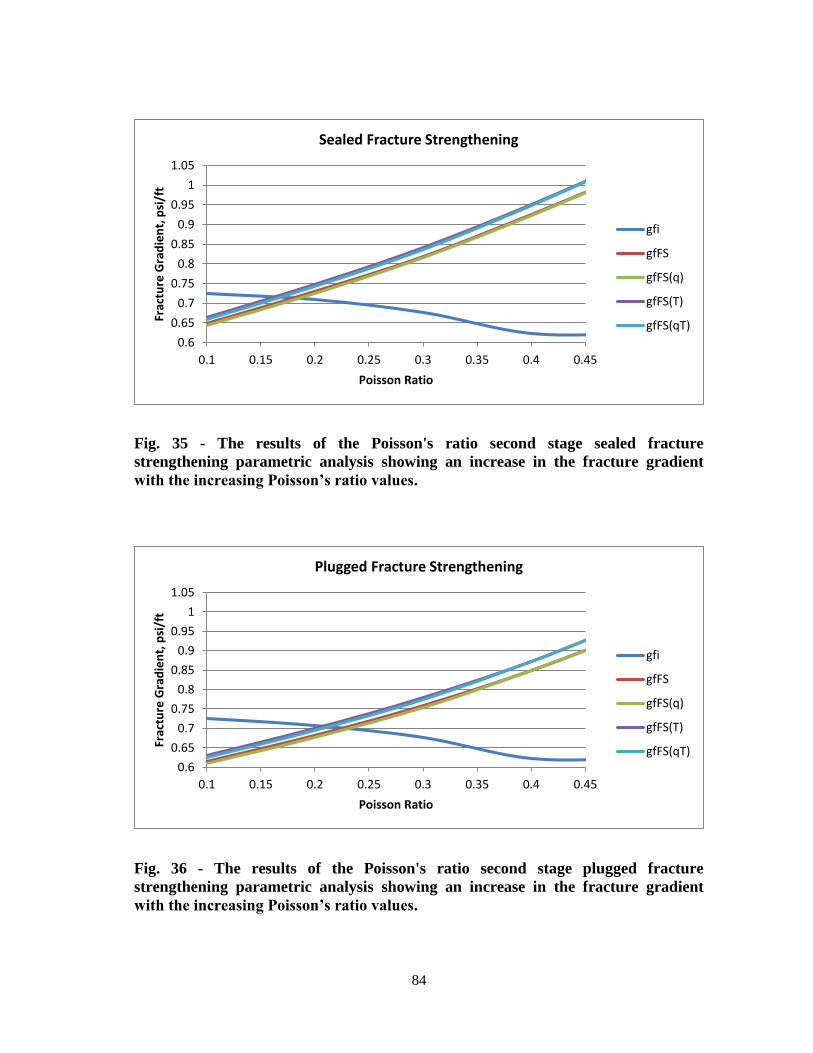
Fig 35 - The results of the Poissons ratio second stage sealed fracture strengthening
parametric analysis showing an increase in the fracture gradient with the
increasing Poissonrsquos ratio values 84
Fig 36 - The results of the Poissons ratio second stage plugged fracture
strengthening parametric analysis showing an increase in the fracture gradient
with the increasing Poissonrsquos ratio values 84
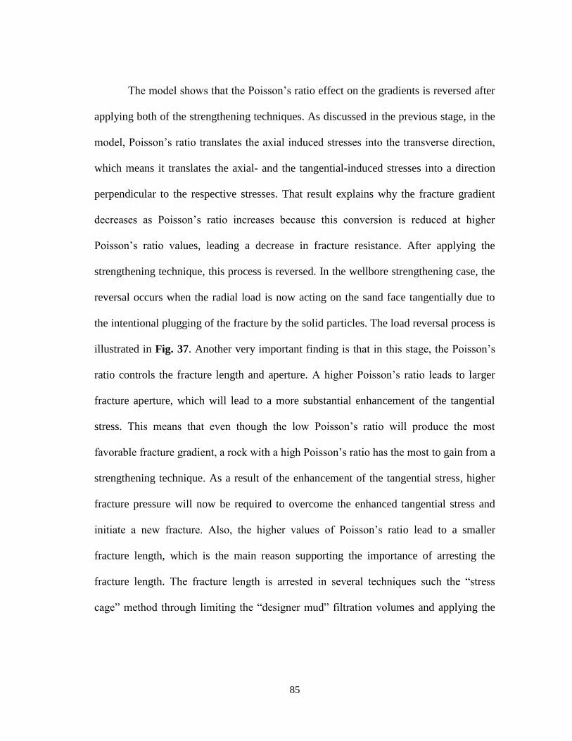
Fig 37 - The illustration of the load reversal after applying the wellbore
strengthening technique due to the action of the Poisson ratio 86
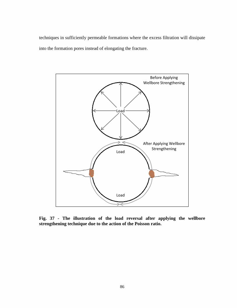
Fig 38 - The results of the Youngs modulus second stage sealed fracture
strengthening parametric analysis showing an increase in the fracture gradient
with the increasing Young modulus values 87
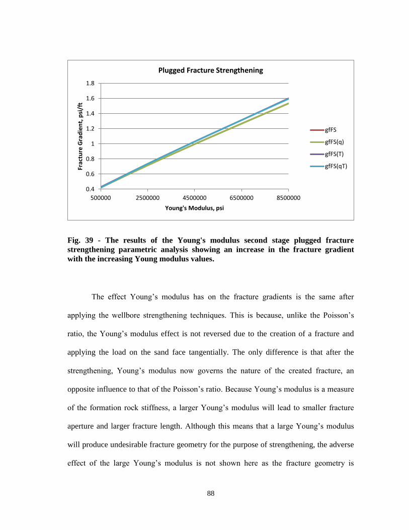
Fig 39 - The results of the Youngs modulus second stage plugged fracture
strengthening parametric analysis showing an increase in the fracture gradient
with the increasing Young modulus values 88
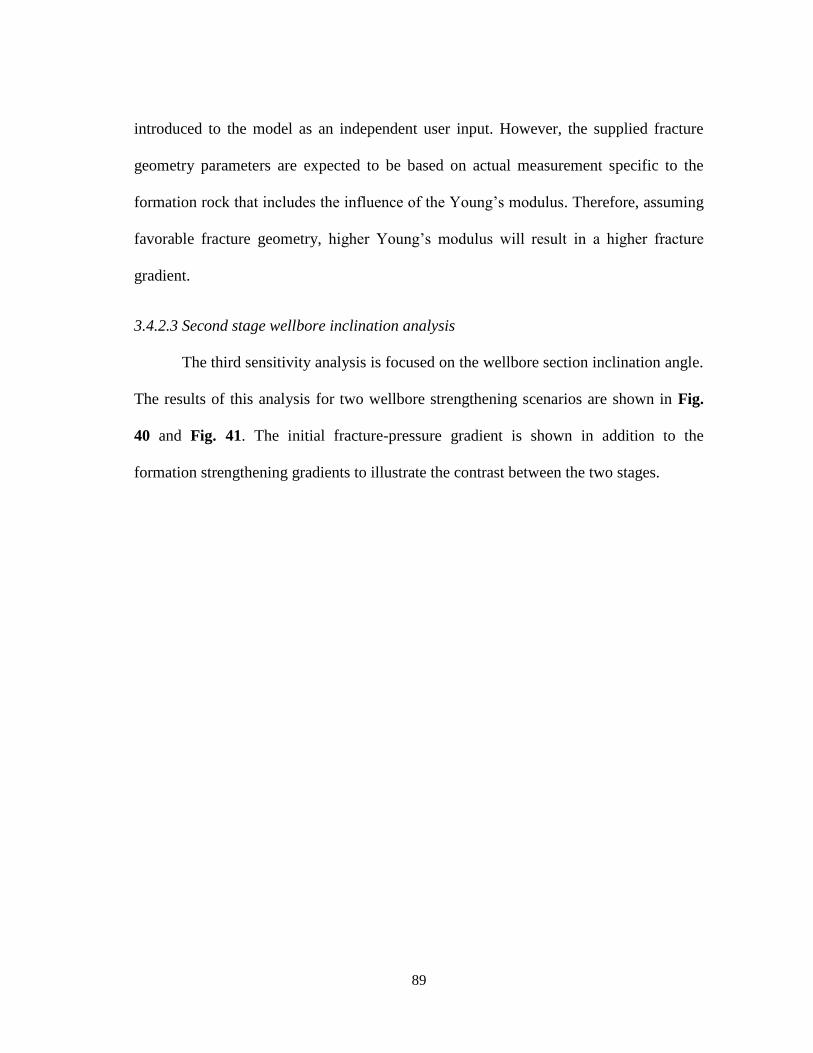
Fig 40 - The results of the wellbore inclination angle second stage sealed fracture
strengthening parametric analysis 90
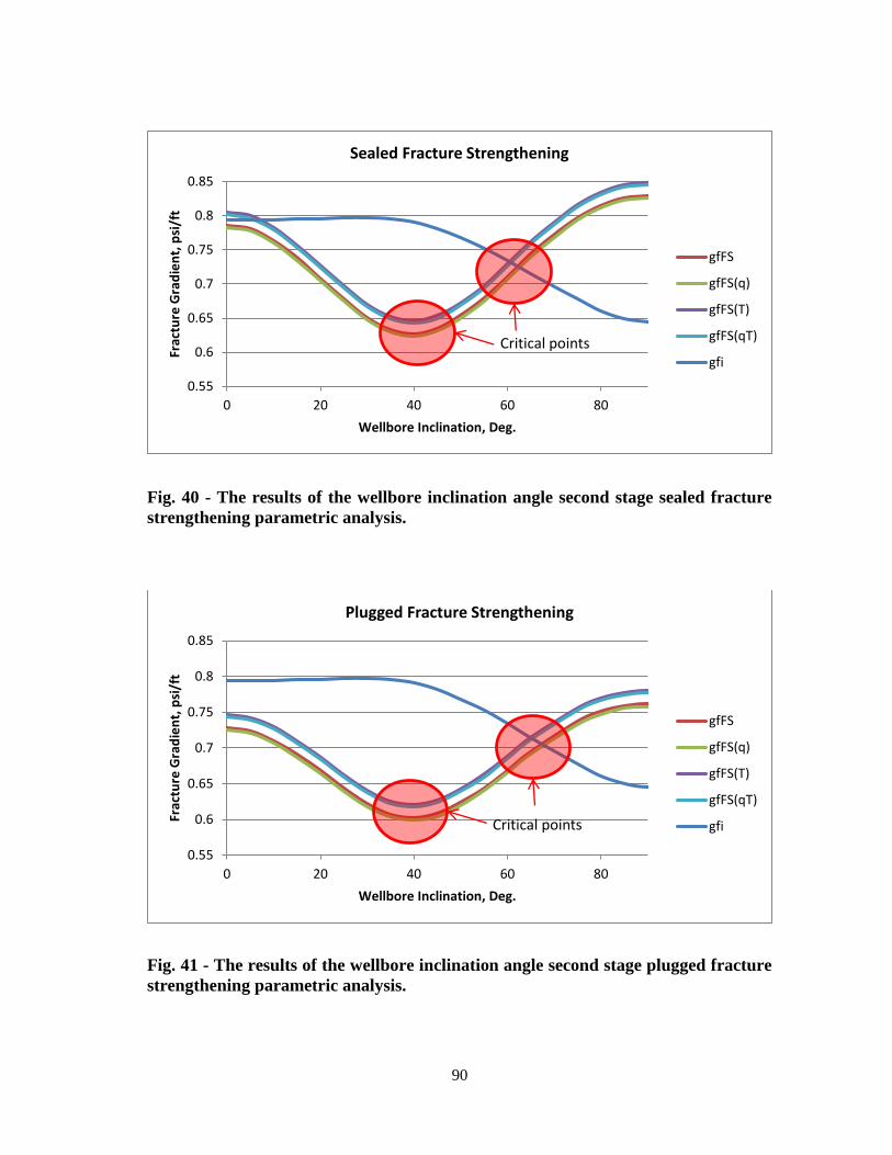
Fig 41 - The results of the wellbore inclination angle second stage plugged fracture
strengthening parametric analysis 90
xi
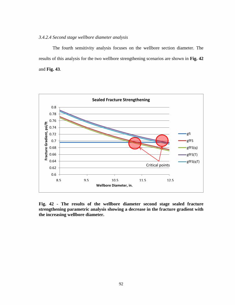
Fig 42 - The results of the wellbore diameter second stage sealed fracture
strengthening parametric analysis showing a decrease in the fracture gradient
with the increasing wellbore diameter 92
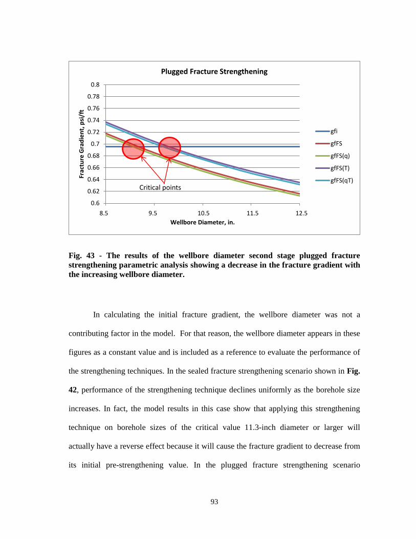
Fig 43 - The results of the wellbore diameter second stage plugged fracture
strengthening parametric analysis showing a decrease in the fracture gradient
with the increasing wellbore diameter 93
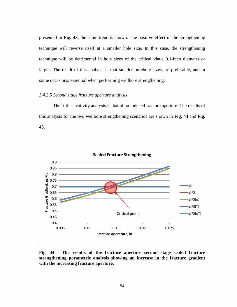
Fig 44 - The results of the fracture aperture second stage sealed fracture
strengthening parametric analysis showing an increase in the fracture gradient
with the increasing fracture aperture 94
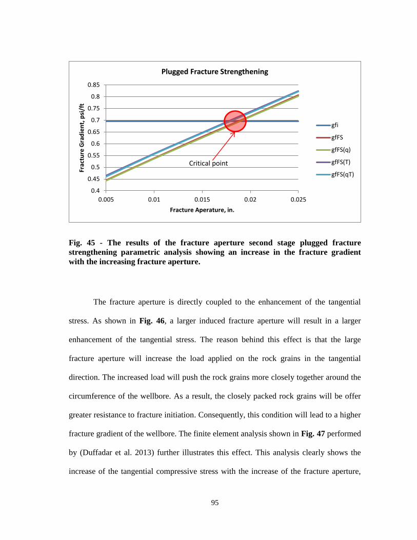
Fig 45 - The results of the fracture aperture second stage plugged fracture
strengthening parametric analysis showing an increase in the fracture gradient
with the increasing fracture aperture 95
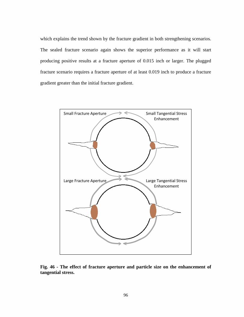
Fig 46 - The effect of fracture aperture and particle size on the enhancement of
tangential stress 96
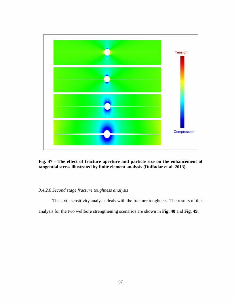
Fig 47 - The effect of fracture aperture and particle size on the enhancement of
tangential stress illustrated by finite element analysis (Duffadar et al 2013) 97
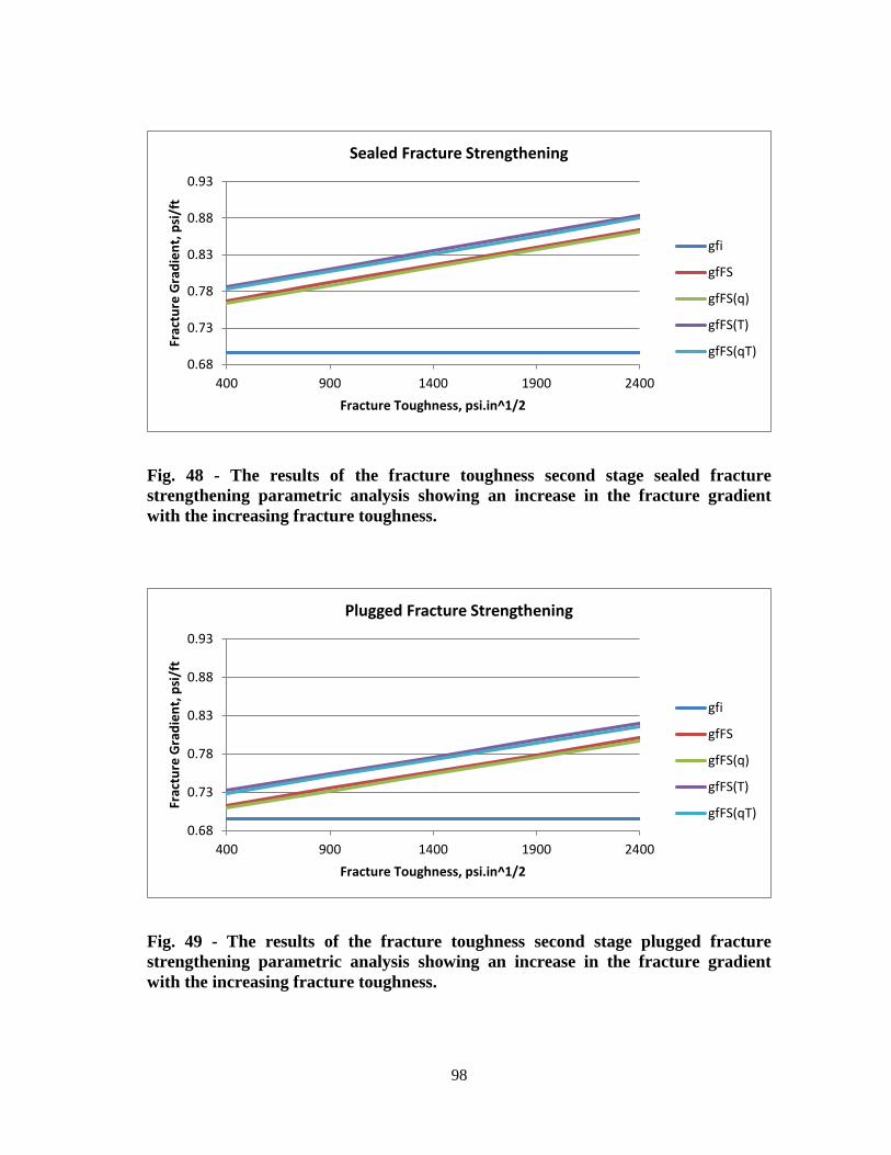
Fig 48 - The results of the fracture toughness second stage sealed fracture
strengthening parametric analysis showing an increase in the fracture gradient
with the increasing fracture toughness 98
Fig 49 - The results of the fracture toughness second stage plugged fracture
strengthening parametric analysis showing an increase in the fracture gradient
with the increasing fracture toughness 98
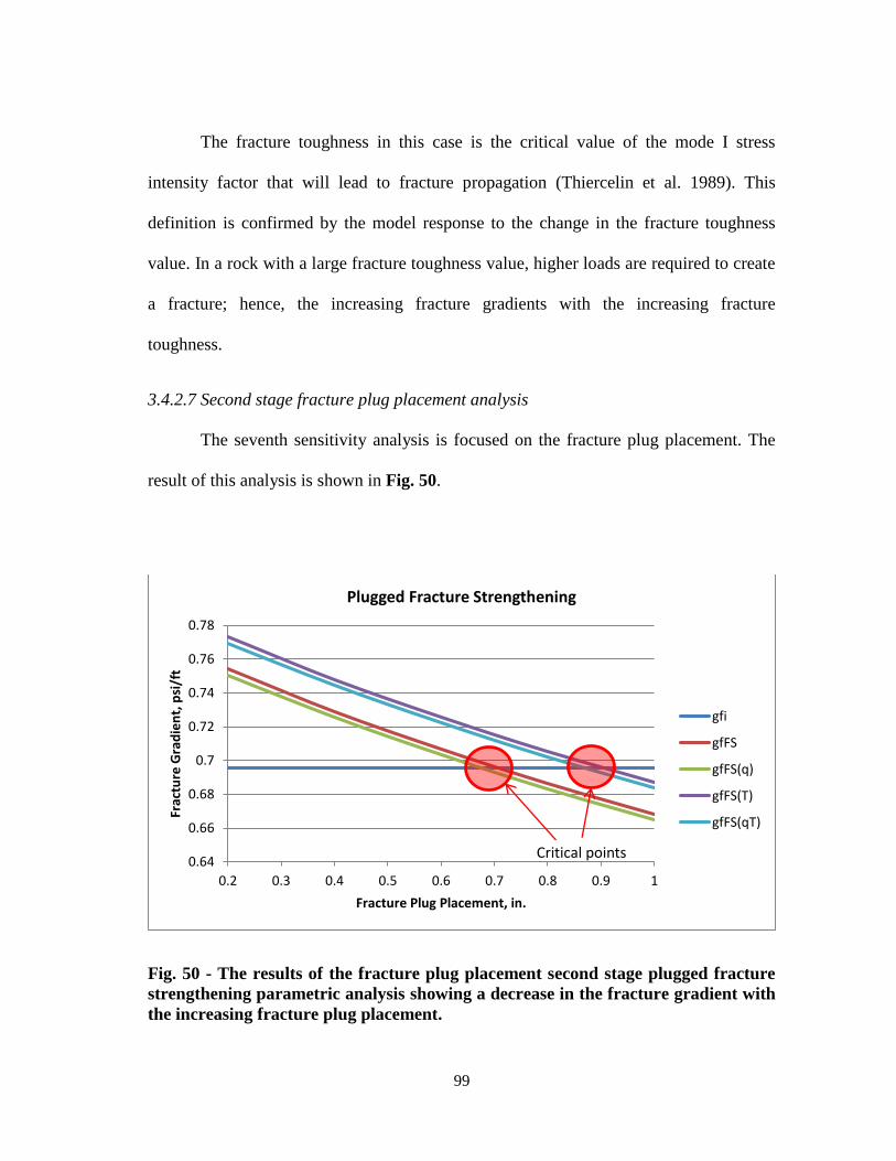
Fig 50 - The results of the fracture plug placement second stage plugged fracture
strengthening parametric analysis showing a decrease in the fracture gradient
with the increasing fracture plug placement 99
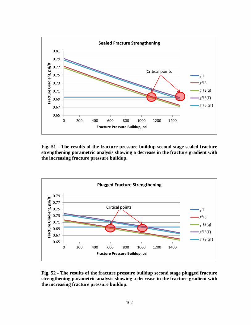
Fig 51 - The results of the fracture pressure buildup second stage sealed fracture
strengthening parametric analysis showing a decrease in the fracture gradient
with the increasing fracture pressure buildup 102
Fig 52 - The results of the fracture pressure buildup second stage plugged fracture
strengthening parametric analysis showing a decrease in the fracture gradient
with the increasing fracture pressure buildup 102
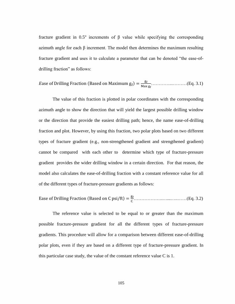
Fig 53 - The resulting ease of drilling plot based on a maximum gradient for the
initial fracture pressure gradient 106
xii
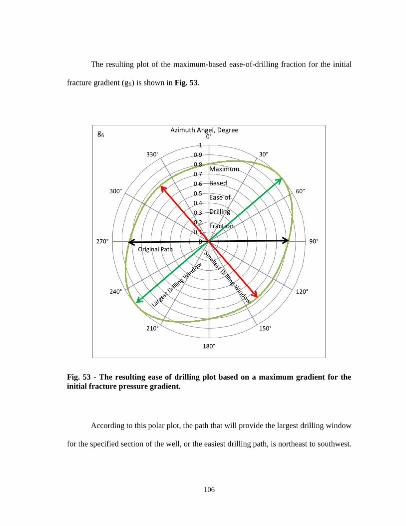
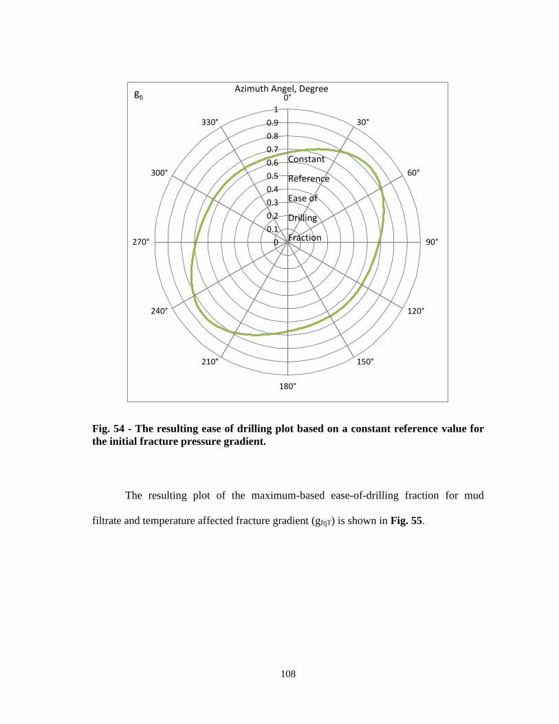
Fig 54 - The resulting ease of drilling plot based on a constant reference value for
the initial fracture pressure gradient 108
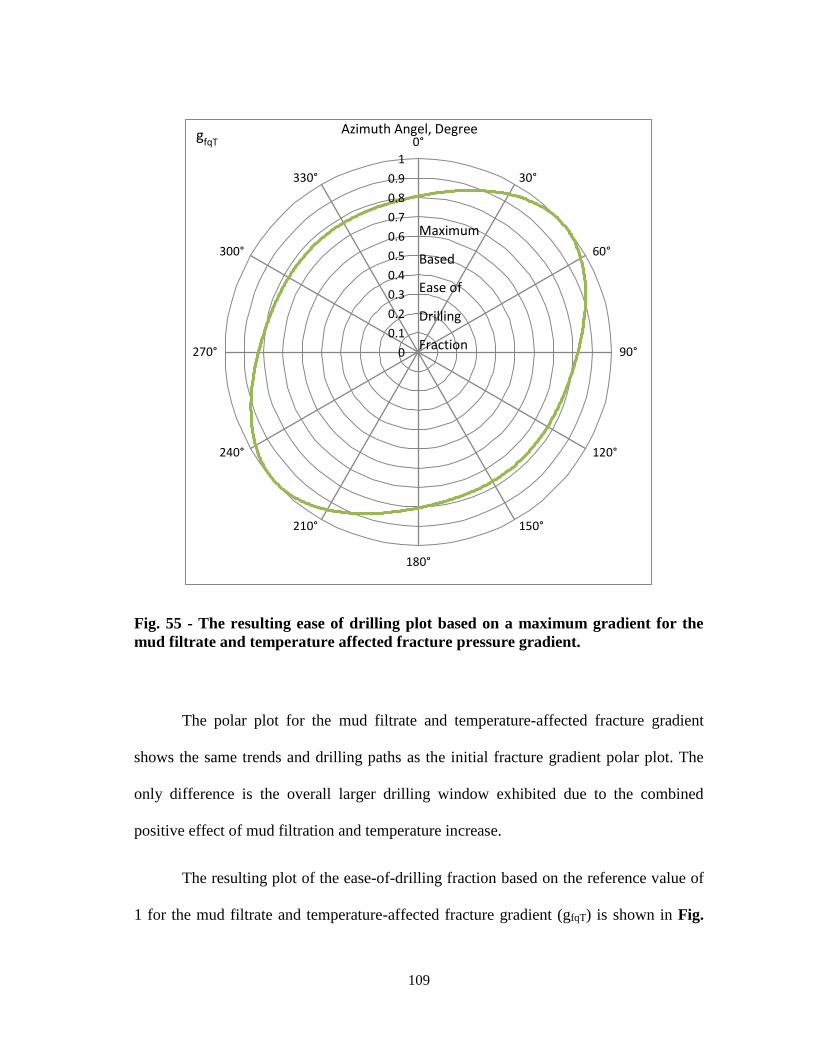
Fig 55 - The resulting ease of drilling plot based on a maximum gradient for the
mud filtrate and temperature affected fracture pressure gradient 109
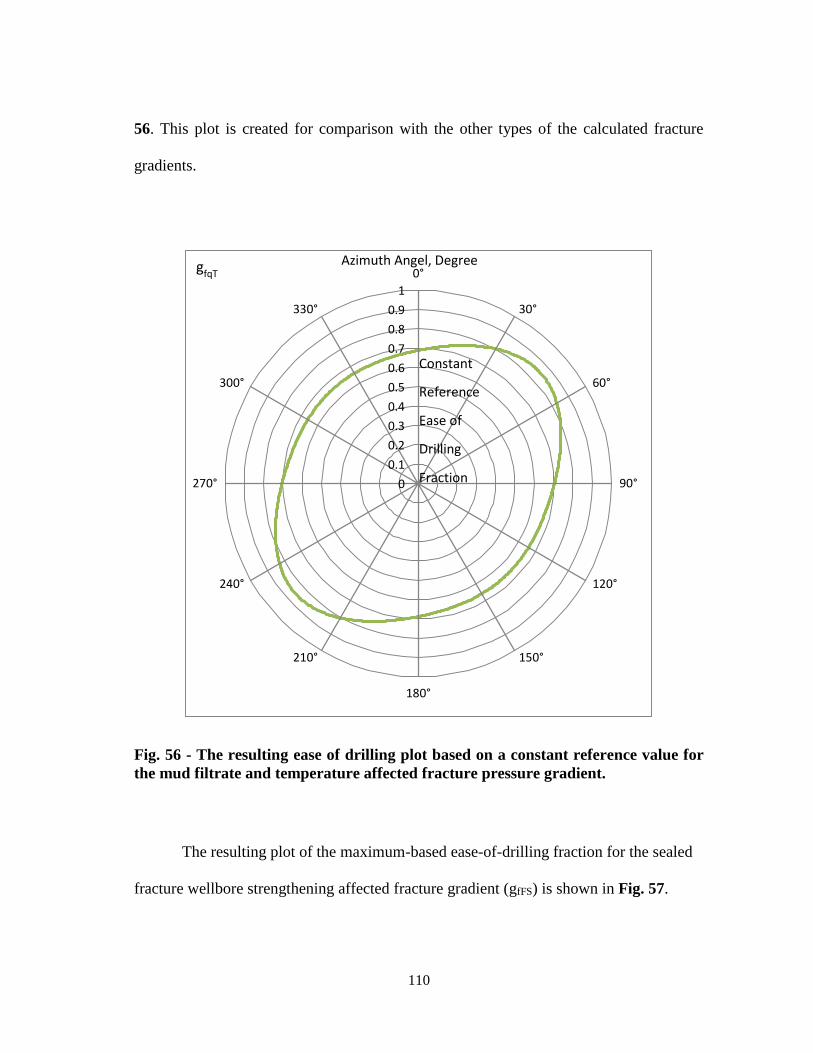
Fig 56 - The resulting ease of drilling plot based on a constant reference value for
the mud filtrate and temperature affected fracture pressure gradient 110
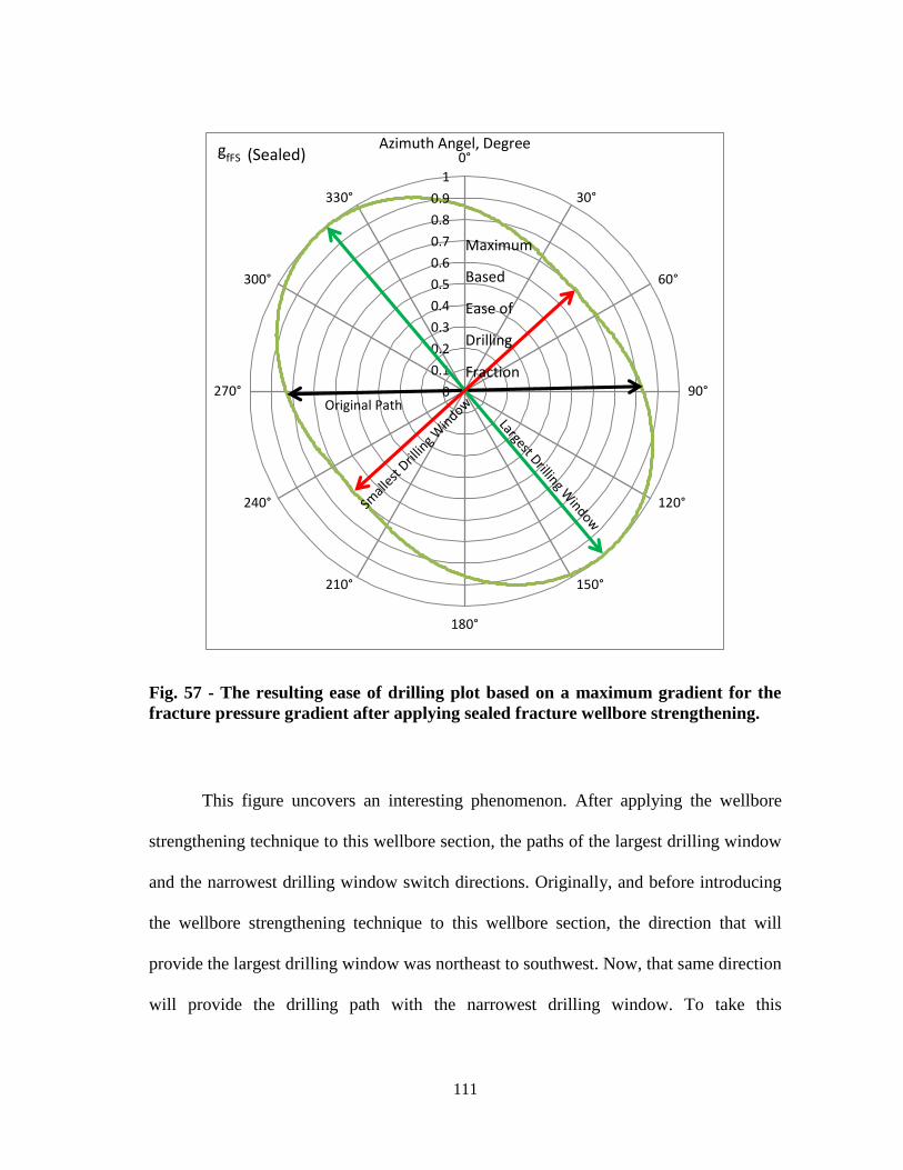
Fig 57 - The resulting ease of drilling plot based on a maximum gradient for the
fracture pressure gradient after applying sealed fracture wellbore
strengthening 111
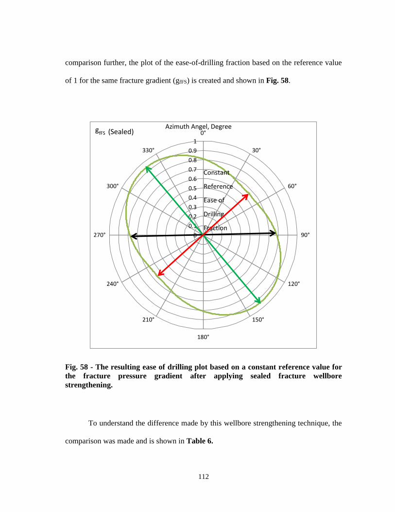
Fig 58 - The resulting ease of drilling plot based on a constant reference value for
the fracture pressure gradient after applying sealed fracture wellbore
strengthening 112
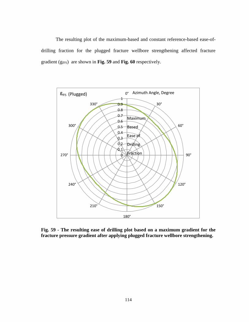
Fig 59 - The resulting ease of drilling plot based on a maximum gradient for the
fracture pressure gradient after applying plugged fracture wellbore
strengthening 114
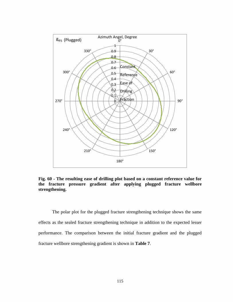
Fig 60 - The resulting ease of drilling plot based on a constant reference value for
the fracture pressure gradient after applying plugged fracture wellbore
strengthening 115
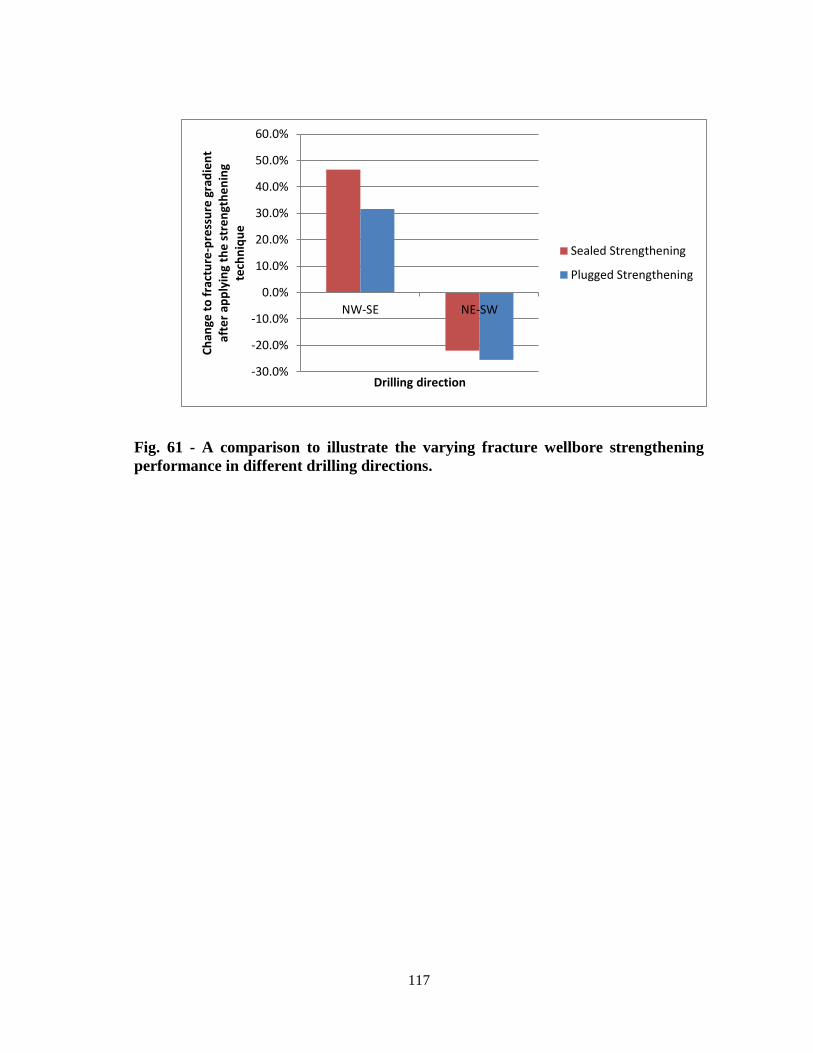
Fig 61 - A comparison to illustrate the varying fracture wellbore strengthening
performance in different drilling directions 117
xiii
LIST OF TABLES
Page
Table 1 - The initial input values for the model case study 64
Table 2 - The model preliminary results 67
Table 3 - Input data describing the interaction between the induced fractures and the
solid particles for the wellbore strengthening part of the model case study 69
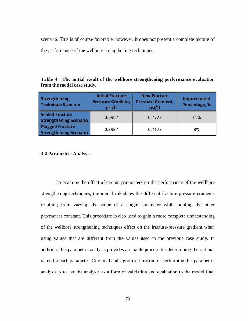
Table 4 - The initial result of the wellbore strengthening performance evaluation
from the model case study 70
Table 5 - The range of Youngs modulus and Poissons ratio used for the parametric
analysis (Fjaer et al 2008) 74
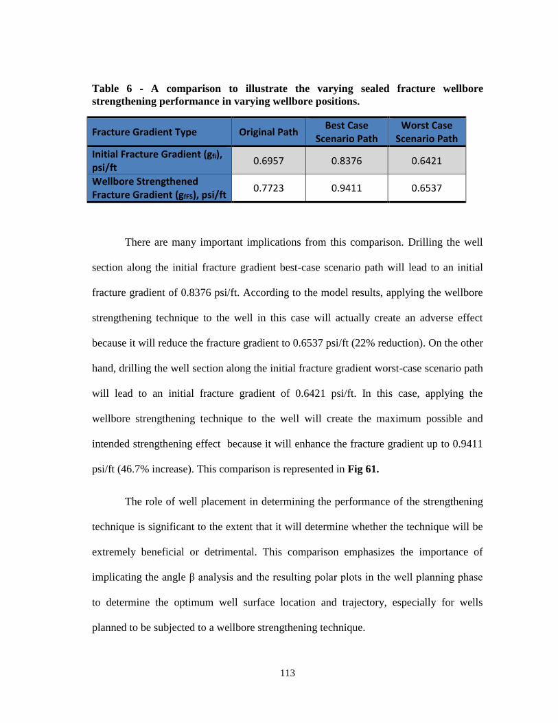
Table 6 - A comparison to illustrate the varying sealed fracture wellbore
strengthening performance in varying wellbore positions 113
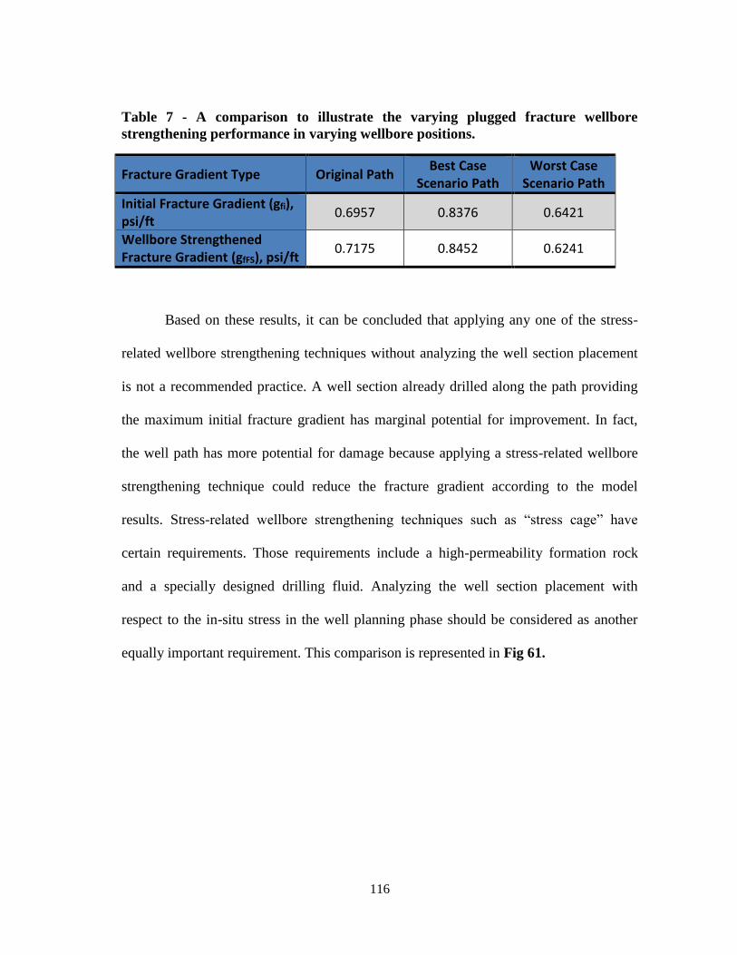
Table 7 - A comparison to illustrate the varying plugged fracture wellbore
strengthening performance in varying wellbore positions 116
1
1 INTRODUCTION
11 Wellbore Strengthening Definition
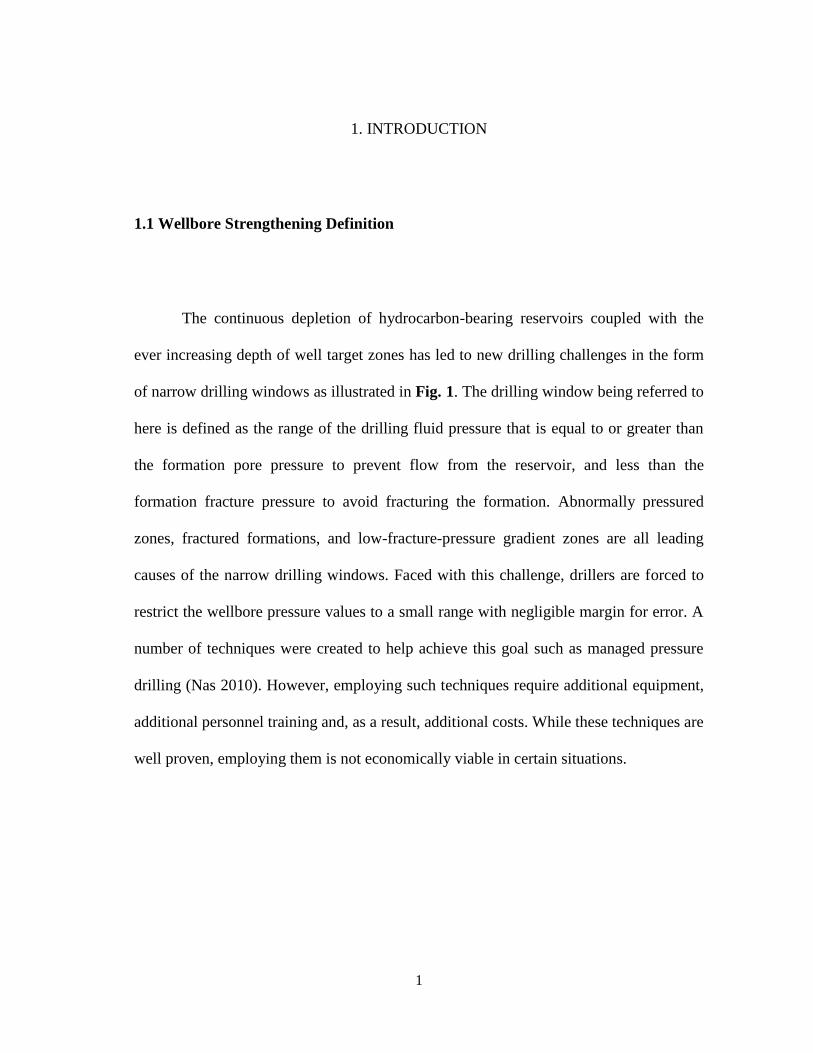
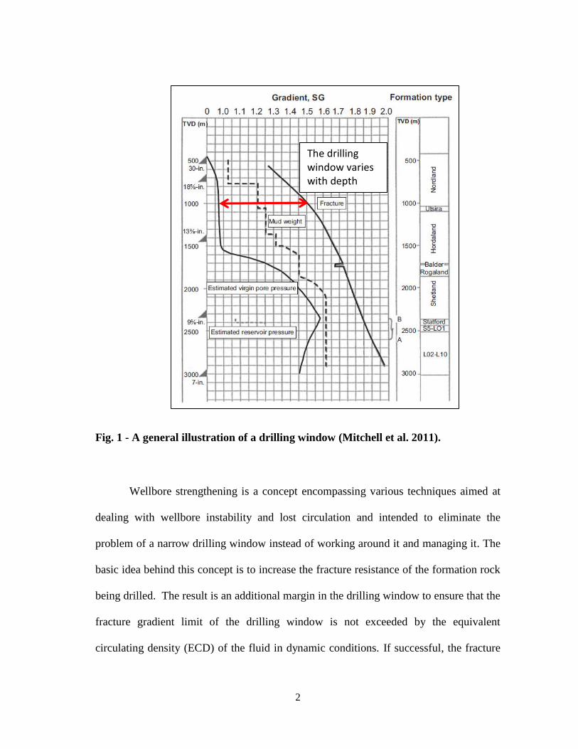
The continuous depletion of hydrocarbon-bearing reservoirs coupled with the
ever increasing depth of well target zones has led to new drilling challenges in the form
of narrow drilling windows as illustrated in Fig 1 The drilling window being referred to
here is defined as the range of the drilling fluid pressure that is equal to or greater than
the formation pore pressure to prevent flow from the reservoir and less than the
formation fracture pressure to avoid fracturing the formation Abnormally pressured
zones fractured formations and low-fracture-pressure gradient zones are all leading
causes of the narrow drilling windows Faced with this challenge drillers are forced to
restrict the wellbore pressure values to a small range with negligible margin for error A
number of techniques were created to help achieve this goal such as managed pressure
drilling (Nas 2010) However employing such techniques require additional equipment
additional personnel training and as a result additional costs While these techniques are
well proven employing them is not economically viable in certain situations
2
Fig 1 - A general illustration of a drilling window (Mitchell et al 2011)
Wellbore strengthening is a concept encompassing various techniques aimed at
dealing with wellbore instability and lost circulation and intended to eliminate the
problem of a narrow drilling window instead of working around it and managing it The
basic idea behind this concept is to increase the fracture resistance of the formation rock
being drilled The result is an additional margin in the drilling window to ensure that the
fracture gradient limit of the drilling window is not exceeded by the equivalent
circulating density (ECD) of the fluid in dynamic conditions If successful the fracture
The drilling window varies with depth
3
gradient is sufficiently enhanced to allow for employing drilling fluid with a higher mud
weight
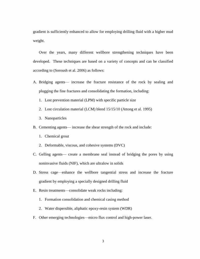
Over the years many different wellbore strengthening techniques have been
developed These techniques are based on a variety of concepts and can be classified
according to (Soroush et al 2006) as follows
A Bridging agentsmdash increase the fracture resistance of the rock by sealing and
plugging the fine fractures and consolidating the formation including
1 Lost prevention material (LPM) with specific particle size
2 Lost circulation material (LCM) blend 151510 (Attong et al 1995)
3 Nanoparticles
B Cementing agentsmdash increase the shear strength of the rock and include
1 Chemical grout
2 Deformable viscous and cohesive systems (DVC)
C Gelling agentsmdash create a membrane seal instead of bridging the pores by using
noninvasive fluids (NIF) which are ultralow in solids
D Stress cagemdashenhance the wellbore tangential stress and increase the fracture
gradient by employing a specially designed drilling fluid
E Resin treatmentsmdashconsolidate weak rocks including
1 Formation consolidation and chemical casing method
2 Water dispersible aliphatic epoxy-resin system (WDR)
F Other emerging technologiesmdashmicro flux control and high-power laser
4
12 Objectives
This work focuses on a certain range of wellbore strengthening techniques This
range includes all of the wellbore strengthening techniques that use the stress state
around the wellbore as the main criteria for enhancing the fracture gradient These
wellbore strengthening techniques include bridging agents and LCM the stress cage
concept and wellbore drilling fluid temperature variations
The main goal of this work is to examine the performance of the defined
wellbore strengthening techniques and predict the final results from implementing these
techniques The evaluation of their performance is based on geometric principles basic
rock mechanics data linear elasticity plane stress theory drilling fluid data and
geological data A code and a user-friendly interface is created in VBA Excelreg
programming language based on the sets of data and principles listed previously in
addition to the use of a recent and reputable numerical solution
The secondary objective in this work is to provide a practical and accessible tool
to be used in evaluating and predicting the performance of a specific wellbore
strengthening technique in a particular section of a well The tool is intended to be used
in the well planning phase on a well section expected to cause drilling troubles such as
lost circulation and hole stability issues due to a narrow drilling window It will help to
determine the applicability of a particular wellbore strengthening technique Another
important goal is reducing the cost of drilling problems either by defining the most
5
applicable wellbore strengthening technique for the situation or by avoiding the use of a
particular wellbore strengthening technique due to predicted poor performance
The final goal is to enable the proper selection of well candidates for wellbore
strengthening based on a thorough study of different scenarios These scenarios are
created to reveal the best well candidate for wellbore strengthening in a certain field
based on its placement trajectory and surface location This method will help to obtain
the maximum possible performance out of the selected wellbore strengthening
techniques
6
2 MODEL DESCRIPTION
21 Model Introduction
The purpose of this model is to combine the use of geometric principles rock
mechanics linear elasticity plane stress theory and geological data to estimate the initial
virgin fracture-pressure gradient in a certain section of a well The model is then
extended to evaluate the stress state and stress-related wellbore strengthening techniques
through the use of recently available and reputable numerical solutions
This model relies primarily on the tangential (hoop stress) concept first described
by (Kirsch 1898) The model is based on the concept that a fracture in a wellbore is first
initiated when the effective tangential stress or hoop stress is reduced to zero by the
wellbore pressure provided the wellbore pressure overcomes the additional and usually
marginal rock tensile strength This concept is the main principle used to estimate the
initial virgin fracture-pressure gradient and the affect In the next step fundamental
wellbore parameters including change in temperature due to the drilling fluid and
wellbore rock contact and change in local pore pressure due to filtration are examined to
illustrate their effect on tangential stress and consequently on the fracture-pressure
gradient
7
Another concept used in the model is the fracture propagation concept
According to this concept an already initiated fracture can propagate when the wellbore
pressure exceeds the minimum field stress and the additional fracture toughness This the
main basis for the wellbore strengthening techniques evaluation portion of the model
A programming code is created to combine these concepts into a single model
that can be used to evaluate the wellbore strengthening (fracture-pressure gradient
enhancement) potential and applicability in a particular section of a well specifically
defined by its depth pore pressure in-situ stress rock properties inclination azimuth
and position with respect to the in-situ stress field
22 In-Situ Stress Transformation
221 In-Situ Stress Description
For the purpose of quantifying the initial or virgin fracture-pressure gradient the
earth in-situ stresses are transformed to the wellbore coordinate system First the earth
in-situ stresses need to be measured or estimated and described Due to the fact that rock
masses are rarely homogeneous as well as the fact that the state of the stress is the result
of consequential past geological events in-situ stresses are almost impossible to measure
precisely and are always changing with time (Amadei et al 1997a) Therefore
8
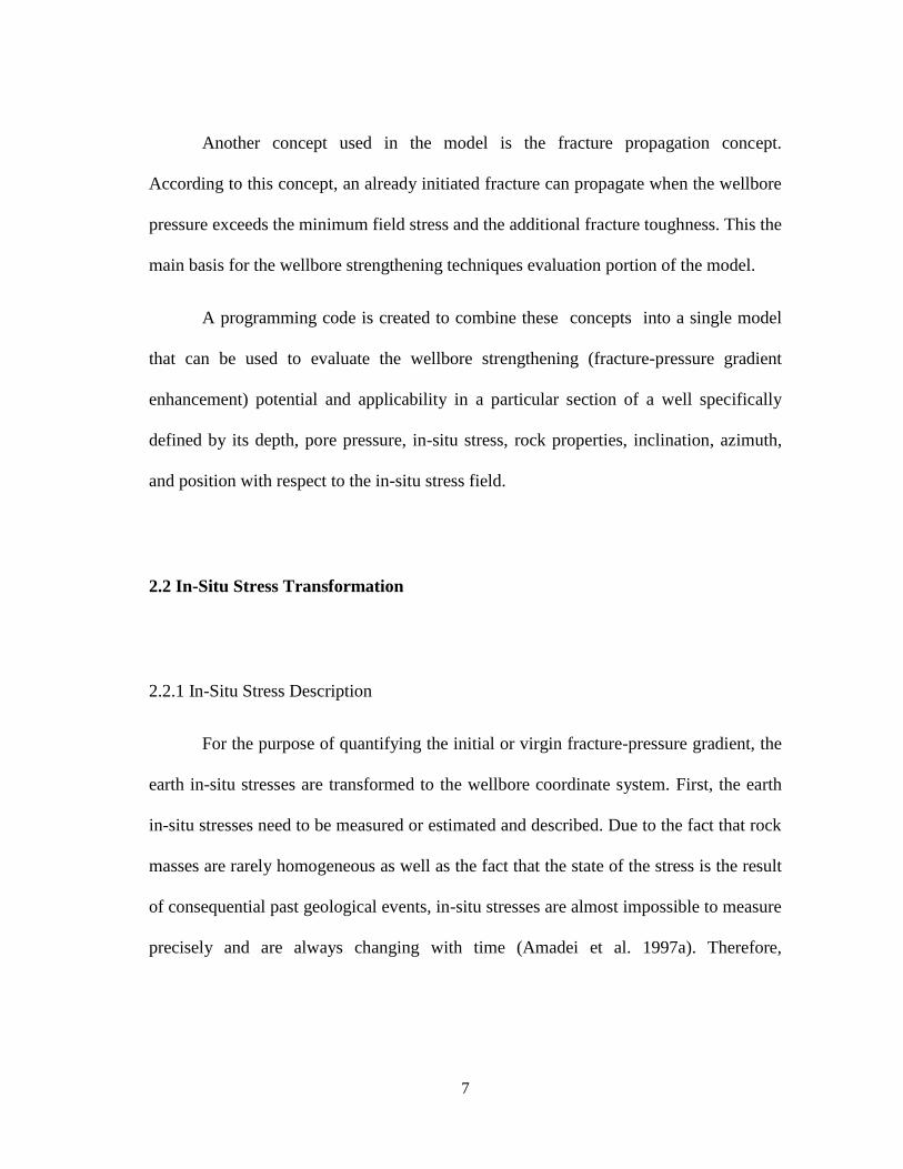
estimating those stresses from stress versus depth relationships is a more common
process than actually measuring them
Fig 2 - The world in-situ stress map showing direction and magnitude of stresses
(Tingay et al 2006)
A good starting point for achieving the goal of describing in-situ stresses is to use
a stress map of the region of interest Through a stress map similar to the one shown in
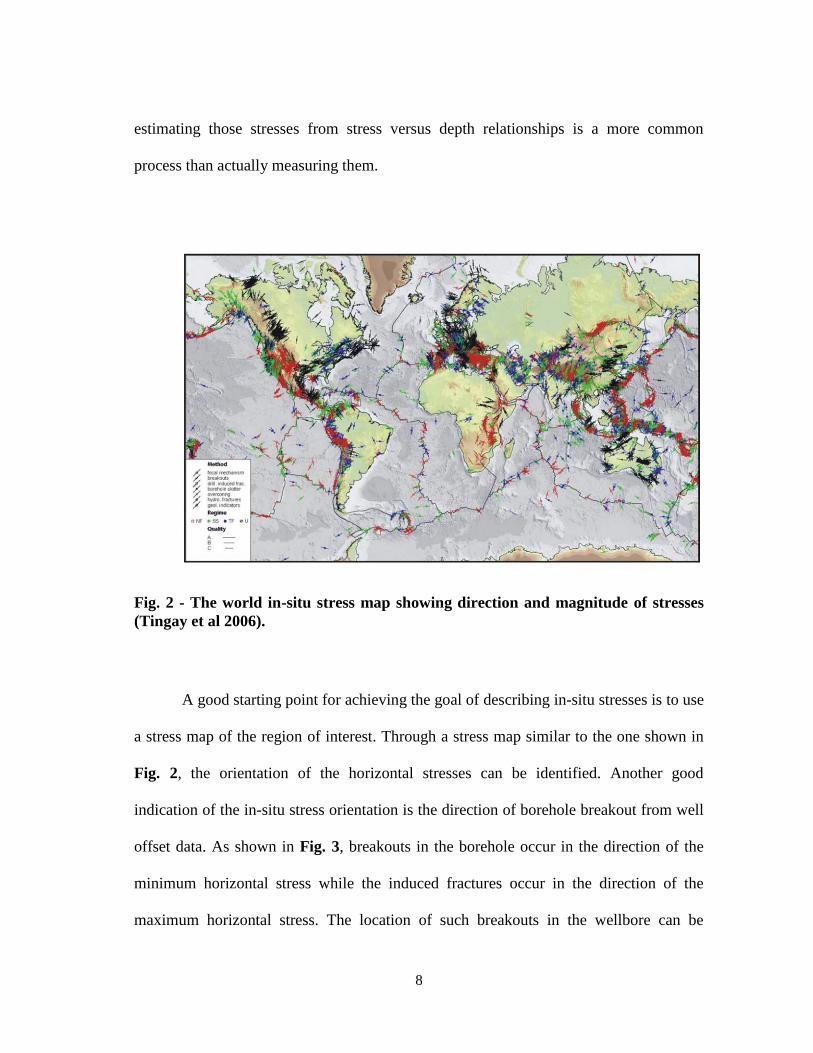
Fig 2 the orientation of the horizontal stresses can be identified Another good
indication of the in-situ stress orientation is the direction of borehole breakout from well
offset data As shown in Fig 3 breakouts in the borehole occur in the direction of the
minimum horizontal stress while the induced fractures occur in the direction of the
maximum horizontal stress The location of such breakouts in the wellbore can be
9
obtained using various types of caliper logs and image logs Well logs perform an
important role in determining the magnitude of the in-situ stresses in addition to the
orientation Density logs provide useful data for estimating the vertical or overburden
stress by calculating the vertical weight above the zone of interest As for the magnitude
of the two horizontal stresses there are countless methods available for obtaining the
magnitude of the two horizontal stresses One method uses the overburden stress pore
pressure and the Poissonrsquos ratio to calculate a single and theoretical nominal value for
the horizontal stress as follows according to (Watson et al 2003)
σH =v
1minusv(σV minus Pp) + Pphelliphelliphelliphelliphelliphelliphelliphelliphelliphelliphelliphelliphelliphelliphelliphelliphelliphelliphelliphellip(Eq 21)
Fig 3 - The pattern of borehole breakout and induced fractures on reference to the
direction of the earth in-situ stresses direction (Dupreist et al 2008)
10
However the method which uses equation 21 is insufficient particularly in
fields with high-horizontal stress anisotropy A more accurate and practical method
involves using borehole opening pressure from the available leakoff test data to estimate
the minimum horizontal stress It is noteworthy that the magnitude of the maximum
horizontal stress is the one that usually has the highest uncertainty of the three in-situ
stresses especially when estimated from the hole ovality (deviation from a circular
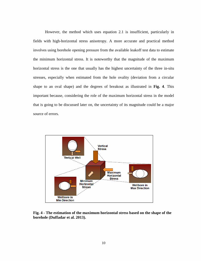
shape to an oval shape) and the degrees of breakout as illustrated in Fig 4 This
important because considering the role of the maximum horizontal stress in the model
that is going to be discussed later on the uncertainty of its magnitude could be a major
source of errors
Fig 4 - The estimation of the maximum horizontal stress based on the shape of the
borehole (Duffadar et al 2013)
11
All of the aforementioned methods should suffice for the purpose of this model
However it should be noted that the in-situ stress values supplied for the model are
expected to be major sources of error and deviation from the actual field values for the
simulated fracture-pressure gradient and the estimation of its enhancement For the
purpose of this model the magnitude and orientation of the earth in-situ stresses are
assumed to be provided
222 The Transformation to the Wellbore Coordinates
The simplest case that the model considers is when the wellbore axis is parallel
to the maximum in-situ stress which in most cases is the vertical overburden pressure
In this case the section of the well being considered is vertical and no in-situ stress
transformation is required because all of the stresses vertical and horizontal are aligned
conveniently with the wellbore axis However for the more common cases where the
wellbore axis in the section being considered deviates at an angle of inclination from the
maximum in-situ stress or the less common cases where the maximum in-situ stress is
not the vertical overburden as in the shallower sections of the well the stresses need to
be converted or transformed to the wellbore coordinate system This transformation
enables the model to quantify the principle in-situ stress components in the direction of
the wellbore axis in the form of converted stresses acting orthogonally to the wellbore
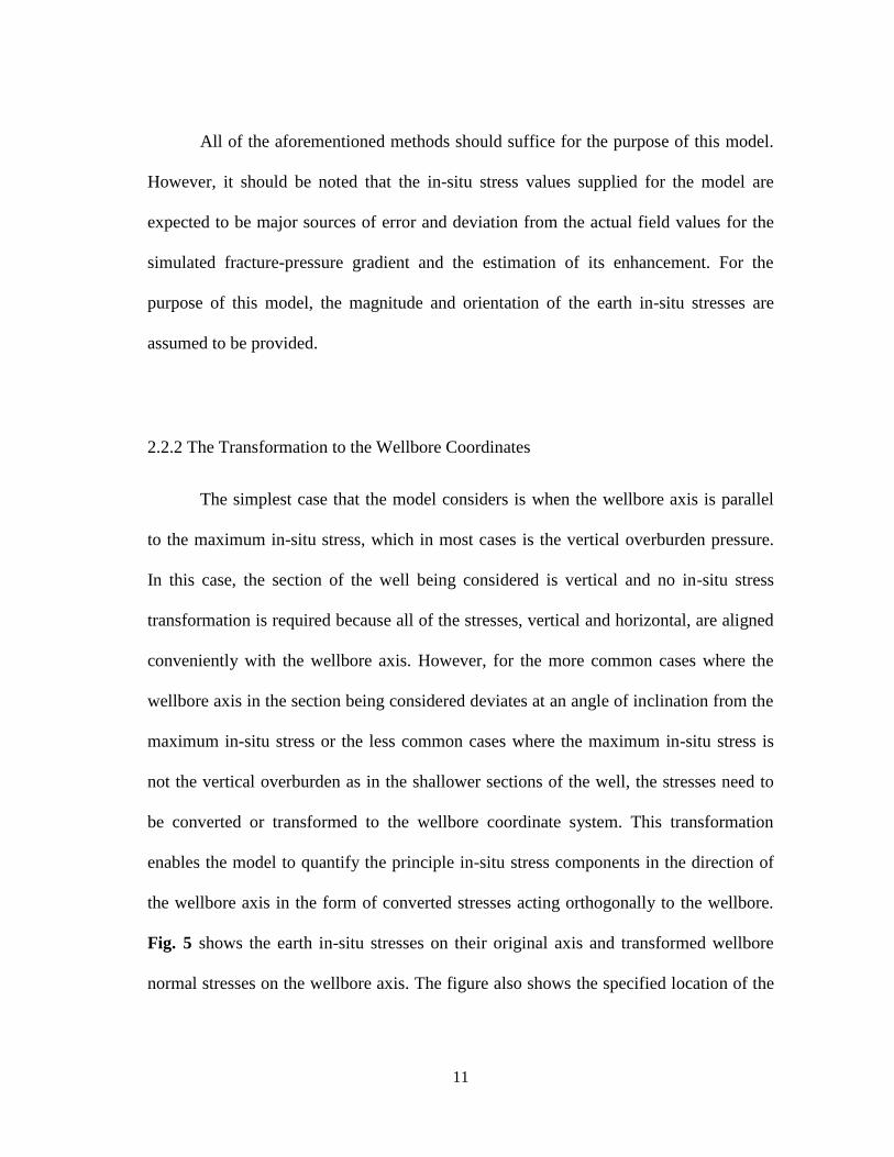
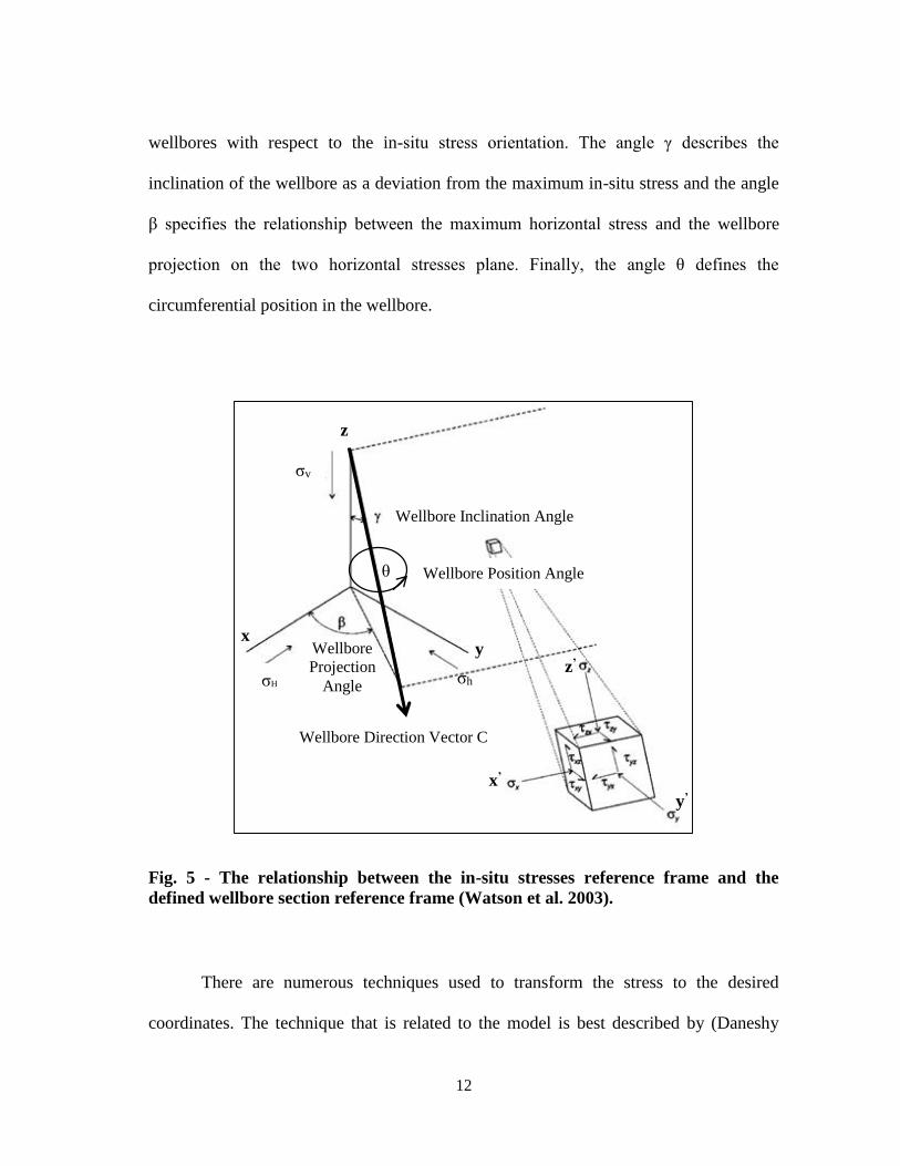
Fig 5 shows the earth in-situ stresses on their original axis and transformed wellbore
normal stresses on the wellbore axis The figure also shows the specified location of the
12
wellbores with respect to the in-situ stress orientation The angle γ describes the
inclination of the wellbore as a deviation from the maximum in-situ stress and the angle
β specifies the relationship between the maximum horizontal stress and the wellbore
projection on the two horizontal stresses plane Finally the angle θ defines the
circumferential position in the wellbore
Fig 5 - The relationship between the in-situ stresses reference frame and the
defined wellbore section reference frame (Watson et al 2003)
There are numerous techniques used to transform the stress to the desired
coordinates The technique that is related to the model is best described by (Daneshy
Wellbore Direction Vector C
σv
Wellbore Inclination Angle
σH σh
Wellbore
Projection
Angle
θ Wellbore Position Angle
z
x y
zrsquo
yrsquo
xrsquo
13
1973) and (Richardson 1983) Using the angles and the coordinate systems described in
Fig 5 the relationship between the in-situ stress coordinates (x y z) and the wellbore
coordinates (xrsquo yrsquo zrsquo) can be established C is the unit vector acting along the wellbore
axis The matrix [σ] defines the in-situ stress components to be transformed What
follows is Richardsonrsquos transformation slightly modified and applied to fit the purpose
of the model
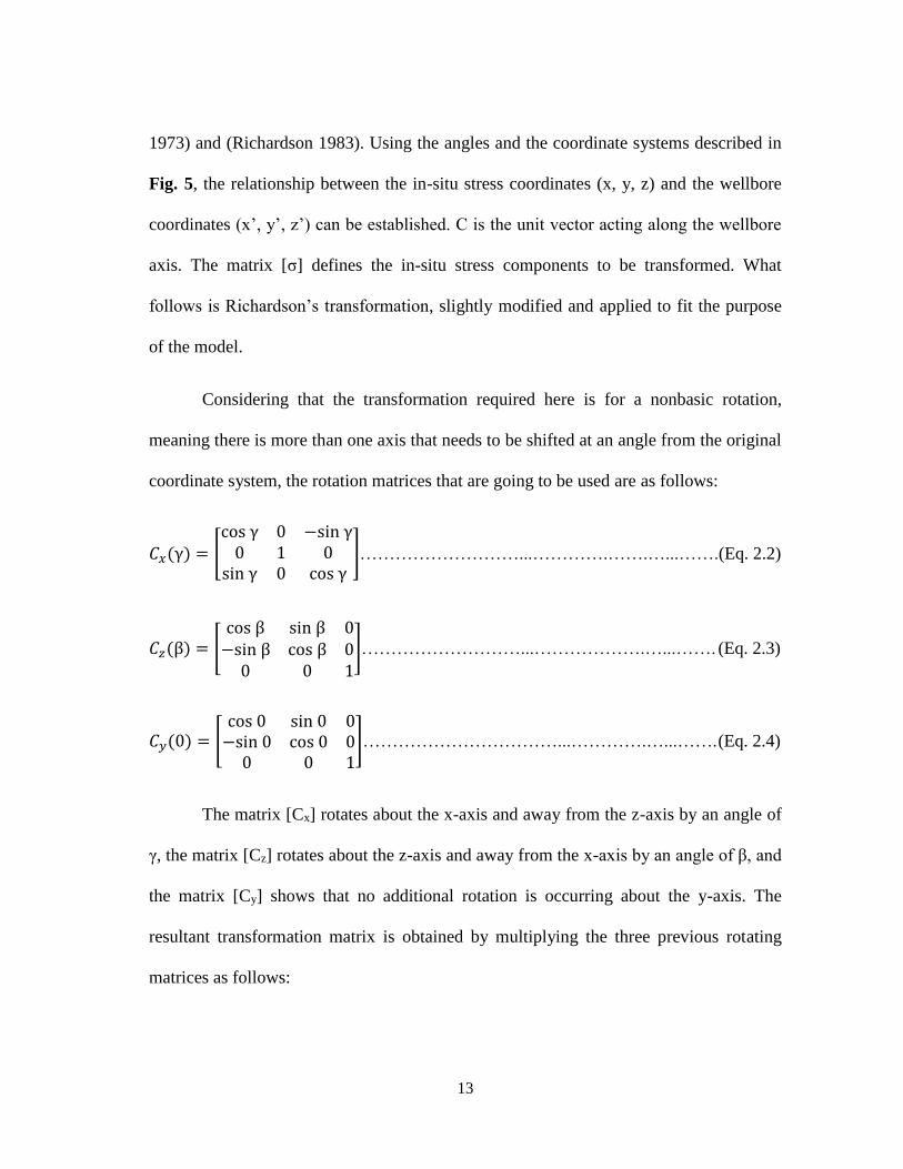
Considering that the transformation required here is for a nonbasic rotation
meaning there is more than one axis that needs to be shifted at an angle from the original
coordinate system the rotation matrices that are going to be used are as follows
119862119909(γ) = [cos γ 0 minussin γ
0 1 0sin γ 0 cos γ
]helliphelliphelliphelliphelliphelliphelliphelliphelliphelliphelliphelliphelliphelliphelliphelliphelliphellip(Eq 22)
119862119911(β) = [cos β sin β 0
minussin β cos β 00 0 1
]helliphelliphelliphelliphelliphelliphelliphelliphelliphelliphelliphelliphelliphelliphelliphelliphelliphellip (Eq 23)
119862119910(0) = [cos 0 sin 0 0
minussin 0 cos 0 00 0 1
]helliphelliphelliphelliphelliphelliphelliphelliphelliphelliphelliphelliphelliphelliphelliphelliphelliphellip (Eq 24)
The matrix [Cx] rotates about the x-axis and away from the z-axis by an angle of
γ the matrix [Cz] rotates about the z-axis and away from the x-axis by an angle of β and
the matrix [Cy] shows that no additional rotation is occurring about the y-axis The
resultant transformation matrix is obtained by multiplying the three previous rotating
matrices as follows
14
[C] = [Cy][Cz][Cx]helliphelliphelliphelliphelliphelliphelliphelliphelliphelliphelliphelliphelliphelliphelliphelliphelliphelliphelliphelliphelliphelliphellip(Eq 25)
Therefore
[cos 0 sin 0 0
minussin 0 cos 0 00 0 1
] [cos γ 0 minussin γ
0 1 0sin γ 0 cos γ
] [cos β sin β 0
minussin β cos β 00 0 1
] =
[
cos γ cos β cos γ sin β minussin γminussin β cos β 0
sin γ cos β sin 120574 sin β cos γ]helliphelliphelliphelliphelliphelliphelliphelliphelliphelliphelliphelliphelliphelliphelliphelliphellip (Eq 26)
The matrix [C] is the second-order transformation for a Cartesian tensor The
final resultant matrix is [σc] which defines the normal wellbore transformed stresses
This matrix can be determined using Cauchyrsquos transformation rule of the stress tensor
According to this rule the stress component in the secondary coordinate system the
wellbore coordinate can be calculated by multiplying the required transformation matrix
[C] by the stress in the original coordinate system matrix the in-situ stress matrix [σ]
and by the transpose of the transformation matrix [C]T as shown in the following
equation
[σc] = [C][σ][C]119879helliphelliphelliphelliphelliphelliphelliphelliphelliphelliphelliphelliphelliphelliphelliphelliphelliphelliphelliphelliphelliphelliphelliphellip (Eq 27)
Therefore
[
σx τxy τxz
τxy σy τyz
τxz τyz σz
] = [
cos γ cos β cos γ sin β minussin γminussin β cos β 0
sin γ cos β sin 120574 sin β cos γ] [
σH 0 00 σh 00 0 σV
]
[
cos γ cos β minussin β sin γ cos βcos γ sin β cos β sin 120574 sin β
minussin γ 0 cos γ]helliphelliphelliphelliphelliphelliphelliphelliphelliphelliphelliphelliphelliphelliphelliphelliphellip(Eq 28)
15
The resulting equations from Cauchyrsquos transformation for each stress term are as
follows
σx = σv sin2γ + (σH cos2 β + σhsin2 β)cos2γhelliphelliphelliphelliphelliphelliphelliphelliphelliphelliphellip (Eq 29)
σy = σHsin2 β + σh cos2 βhelliphelliphelliphelliphelliphelliphelliphelliphelliphelliphelliphelliphelliphelliphelliphelliphelliphellip (Eq 210)
σz = σv cos2γ + (σH cos2 β + σhsin2 β)sin2γhelliphelliphelliphelliphelliphelliphelliphelliphelliphelliphellip (Eq 211)
τyz =σHminusσh
2sin(2120573) sin 120574helliphelliphelliphelliphelliphelliphelliphelliphelliphelliphelliphelliphelliphelliphelliphelliphelliphelliphellip (Eq 212)
τxz =1
2(σH cos2 β + σhsin2 β) sin(2120574)helliphelliphelliphelliphelliphelliphelliphelliphelliphelliphelliphelliphelliphellip (Eq 213)
τxy =σHminusσh
2sin(2120573) cos2γhelliphelliphelliphelliphelliphelliphelliphelliphelliphelliphelliphelliphelliphelliphelliphelliphelliphellip (Eq 214)
These equations do not take into account the effect of rock excavation and the existence
of a borehole they merely transform the in-situ stresses into normal stresses in the
direction of the section of interest in the borehole The removal of the rock through the
drilling process causes a concentration of these wellbore normal stresses in the rock
surrounding the borehole Therefore these stresses are not sufficient for the model to
quantify the fracture-pressure gradient
16
23 Induced Borehole Stresses
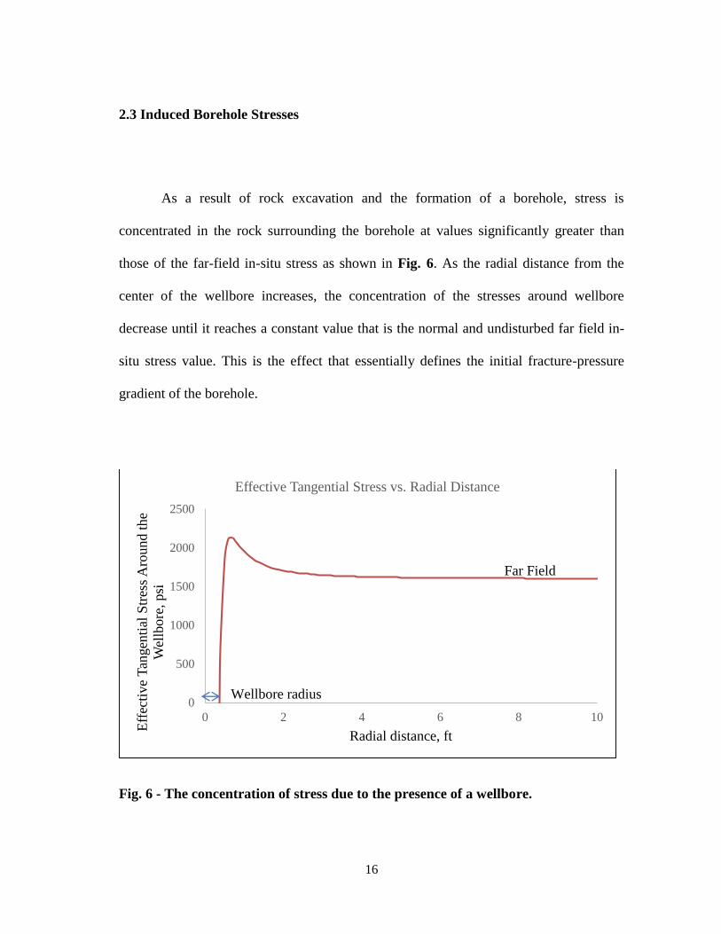
As a result of rock excavation and the formation of a borehole stress is
concentrated in the rock surrounding the borehole at values significantly greater than
those of the far-field in-situ stress as shown in Fig 6 As the radial distance from the
center of the wellbore increases the concentration of the stresses around wellbore
decrease until it reaches a constant value that is the normal and undisturbed far field in-
situ stress value This is the effect that essentially defines the initial fracture-pressure
gradient of the borehole
Fig 6 - The concentration of stress due to the presence of a wellbore
0
500
1000
1500
2000
2500
0 2 4 6 8 10
Eff
ecti
ve
Tan
gen
tial
Str
ess
Aro
und t
he
Wel
lbore
psi
Radial distance ft
Effective Tangential Stress vs Radial Distance
Wellbore radius
(rw)
Far Field
Stress
17
For the purpose of the model these induced stresses need to be quantified based
on the previously determined transformed normal wellbore stresses There are numerous
solutions available for quantifying the induced stresses however the solution required
for this model should agree with its most important rock mechanics assumption which is
linear elasticity In his work published in 1987 Aadonoy provided such a solution
(Aadnoy 1987) It should also be noted that the solution given by the model should yield
a value of induced stresses at the wall of the borehole This point is noteworthy because
there are several solutions available that agree with the model assumption yet they
slightly disagree with models purpose because they aim to determine the induced
stresses of various radial values rather than at the borehole wall This justifies the
selection of the Aadnoyrsquos solution Those solutions are similar to the one used to
produce the plot in Fig 6 (Jaeger et al 2007)
According to Aadnoyrsquos derivation the induced stress should be considered in
three directions It is very important that these directions agree with borehole coordinate
system defined in the previous section for the in-situ stress transformation As a result of
this agreement the value for the transformed stresses can now be used in the model to
quantify the induced stresses instead of directly using the in-situ stresses which would
prove to be substantially in error
The first direction of induced stress is the radial stress which acts on the
borehole walls perpendicular from the center of the borehole The radial stress results
from the hydraulic forces exerted by the drilling fluid occupying the borehole
Therefore the radial stress can be stated simply as the pressure of the wellbore
18
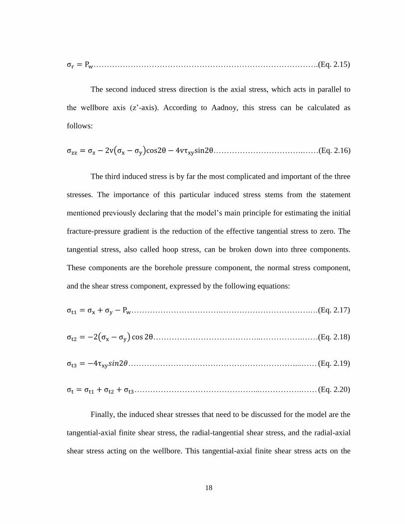
σr = Pwhelliphelliphelliphelliphelliphelliphelliphelliphelliphelliphelliphelliphelliphelliphelliphelliphelliphelliphelliphelliphelliphelliphelliphelliphelliphelliphelliphellip (Eq 215)
The second induced stress direction is the axial stress which acts in parallel to
the wellbore axis (zrsquo-axis) According to Aadnoy this stress can be calculated as
follows
σzz = σz minus 2v(σx minus σy)cos2θ minus 4vτxysin2θhelliphelliphelliphelliphelliphelliphelliphelliphelliphelliphelliphelliphellip(Eq 216)
The third induced stress is by far the most complicated and important of the three
stresses The importance of this particular induced stress stems from the statement
mentioned previously declaring that the modelrsquos main principle for estimating the initial
fracture-pressure gradient is the reduction of the effective tangential stress to zero The
tangential stress also called hoop stress can be broken down into three components
These components are the borehole pressure component the normal stress component
and the shear stress component expressed by the following equations
σt1 = σx + σy minus Pwhelliphelliphelliphelliphelliphelliphelliphelliphelliphelliphelliphelliphelliphelliphelliphelliphelliphelliphelliphelliphelliphelliphellip(Eq 217)
σt2 = minus2(σx minus σy) cos 2θhelliphelliphelliphelliphelliphelliphelliphelliphelliphelliphelliphelliphelliphelliphelliphelliphelliphelliphelliphellip(Eq 218)
σt3 = minus4τxy1199041198941198992120579helliphelliphelliphelliphelliphelliphelliphelliphelliphelliphelliphelliphelliphelliphelliphelliphelliphelliphelliphelliphelliphelliphellip (Eq 219)
σt = σt1 + σt2 + σt3helliphelliphelliphelliphelliphelliphelliphelliphelliphelliphelliphelliphelliphelliphelliphelliphelliphelliphelliphelliphelliphellip (Eq 220)
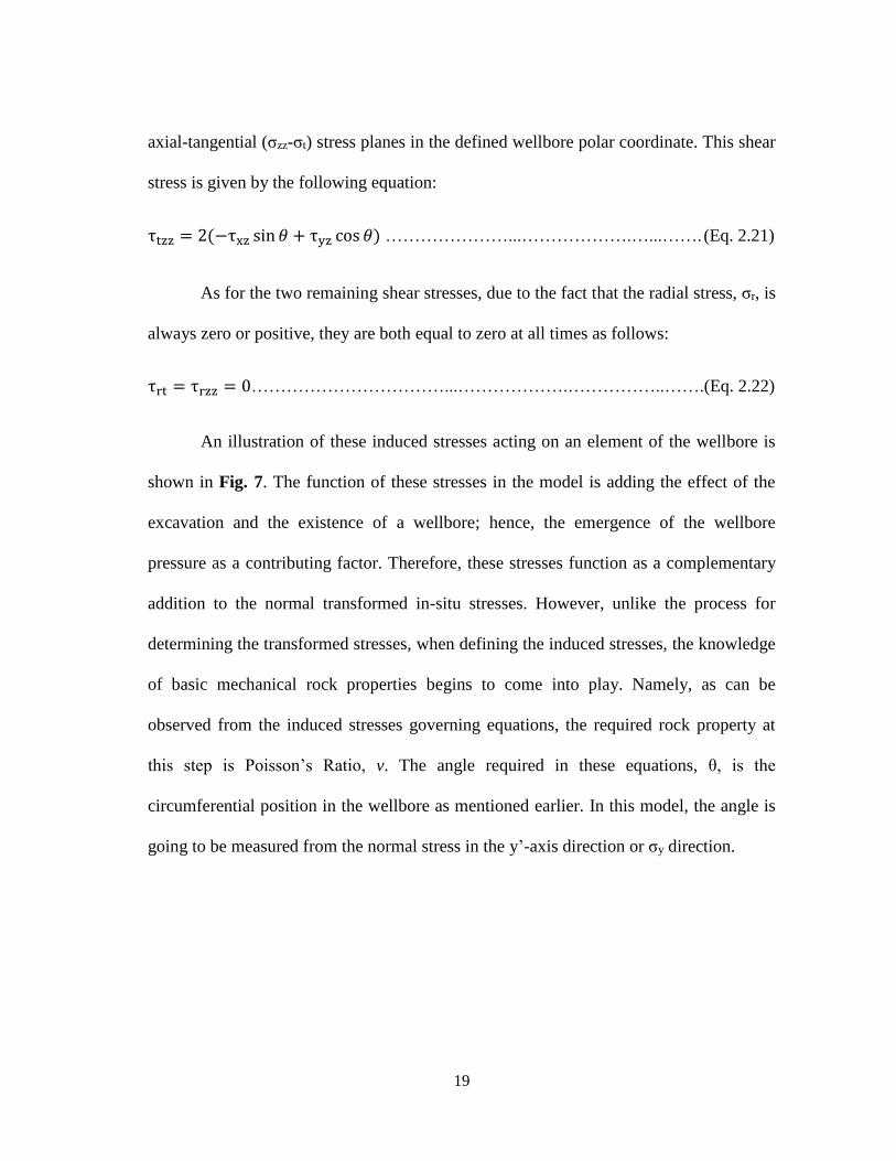
Finally the induced shear stresses that need to be discussed for the model are the
tangential-axial finite shear stress the radial-tangential shear stress and the radial-axial
shear stress acting on the wellbore This tangential-axial finite shear stress acts on the
19
axial-tangential (σzz-σt) stress planes in the defined wellbore polar coordinate This shear
stress is given by the following equation
τtzz = 2(minusτxz sin 120579 + τyz cos 120579) helliphelliphelliphelliphelliphelliphelliphelliphelliphelliphelliphelliphelliphelliphelliphellip (Eq 221)
As for the two remaining shear stresses due to the fact that the radial stress σr is
always zero or positive they are both equal to zero at all times as follows
τrt = τrzz = 0helliphelliphelliphelliphelliphelliphelliphelliphelliphelliphelliphelliphelliphelliphelliphelliphelliphelliphelliphelliphelliphelliphelliphellip(Eq 222)
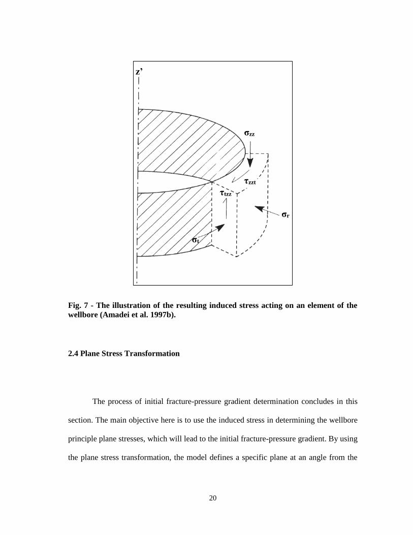
An illustration of these induced stresses acting on an element of the wellbore is
shown in Fig 7 The function of these stresses in the model is adding the effect of the
excavation and the existence of a wellbore hence the emergence of the wellbore
pressure as a contributing factor Therefore these stresses function as a complementary
addition to the normal transformed in-situ stresses However unlike the process for
determining the transformed stresses when defining the induced stresses the knowledge
of basic mechanical rock properties begins to come into play Namely as can be
observed from the induced stresses governing equations the required rock property at
this step is Poissonrsquos Ratio v The angle required in these equations θ is the
circumferential position in the wellbore as mentioned earlier In this model the angle is
going to be measured from the normal stress in the yrsquo-axis direction or σy direction
20
Fig 7 - The illustration of the resulting induced stress acting on an element of the
wellbore (Amadei et al 1997b)
24 Plane Stress Transformation
The process of initial fracture-pressure gradient determination concludes in this
section The main objective here is to use the induced stress in determining the wellbore
principle plane stresses which will lead to the initial fracture-pressure gradient By using
the plane stress transformation the model defines a specific plane at an angle from the
σzz
σt
σr
τtzz
τzzt
zrsquo
21
wellbore axis (2ξp) This plane is the plane of zero shear in the formation which is the
plane that will accommodate the two induced fractures The advantage in adding this
step to the model is that it enables the determination the two stresses (principle stresses
mentioned previously) acting directly on the fracture plane The first of the two stresses
will act perpendicularly to the direction of the induced fractures on the fracture plane
and the second stress will act in the same direction as the induced fractures Recalling
the simple approach undertaken to determine the direction or the position of the wellbore
fracture and wellbore breakout based on the direction of the earth in-situ stresses this
condition can only exist in the case of a simple vertical wellbore with the overburden as
the maximum in-situ stress However changing the wellbore inclination and changing its
position with respect to the in-situ stress renders this approach as being inaccurate at
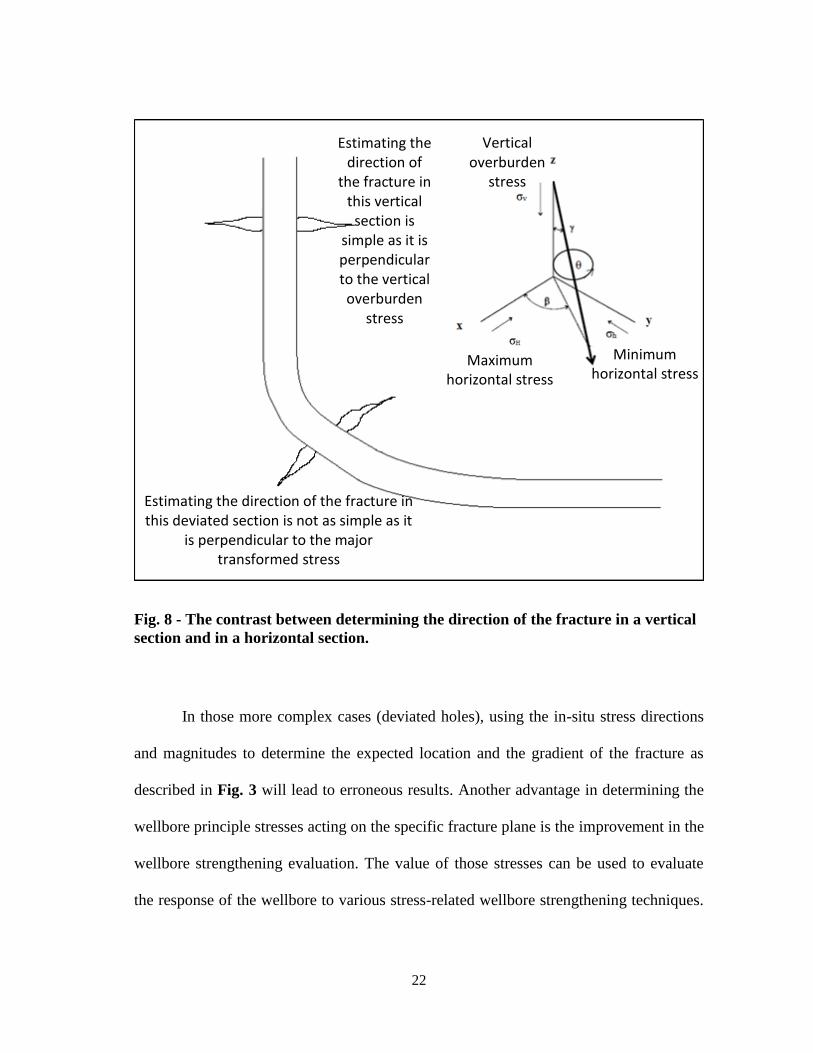
best This contrast between those two scenarios is illustrated in Fig 8
22
Fig 8 - The contrast between determining the direction of the fracture in a vertical
section and in a horizontal section
In those more complex cases (deviated holes) using the in-situ stress directions
and magnitudes to determine the expected location and the gradient of the fracture as
described in Fig 3 will lead to erroneous results Another advantage in determining the
wellbore principle stresses acting on the specific fracture plane is the improvement in the
wellbore strengthening evaluation The value of those stresses can be used to evaluate
the response of the wellbore to various stress-related wellbore strengthening techniques
Maximum horizontal stress
Minimum horizontal stress
Vertical overburden
stress
Estimating the direction of
the fracture in this vertical
section is simple as it is perpendicular to the vertical overburden
stress
Estimating the direction of the fracture in this deviated section is not as simple as it
is perpendicular to the major transformed stress
23
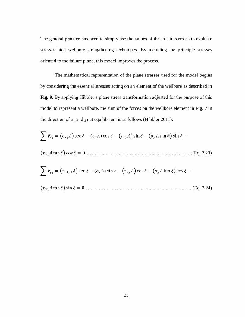
The general practice has been to simply use the values of the in-situ stresses to evaluate
stress-related wellbore strengthening techniques By including the principle stresses
oriented to the failure plane this model improves the process
The mathematical representation of the plane stresses used for the model begins
by considering the essential stresses acting on an element of the wellbore as described in
Fig 9 By applying Hibblerrsquos plane stress transformation adjusted for the purpose of this
model to represent a wellbore the sum of the forces on the wellbore element in Fig 7 in
the direction of x1 and y1 at equilibrium is as follows (Hibbler 2011)
sum 1198651199091= (1205901199091
119860) sec 120585 minus (120590119909119860) cos 120585 minus (120591119909119910119860) sin 120585 minus (120590119910119860 tan 120579) sin 120585 minus
(120591119910119909119860 tan 120585) cos 120585 = 0helliphelliphelliphelliphelliphelliphelliphelliphelliphelliphelliphelliphelliphelliphelliphelliphelliphelliphelliphellip (Eq 223)
sum 1198651199101= (12059111990911199101119860) sec 120585 minus (120590119909119860) sin 120585 minus (120591119909119910119860) cos 120585 minus (120590119910119860 tan 120585) cos 120585 minus
(120591119910119909119860 tan 120585) sin 120585 = 0helliphelliphelliphelliphelliphelliphelliphelliphelliphelliphelliphelliphelliphelliphelliphelliphelliphelliphelliphellip(Eq 224)
24
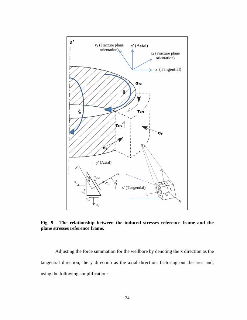
Fig 9 - The relationship between the induced stresses reference frame and the
plane stresses reference frame
Adjusting the force summation for the wellbore by denoting the x direction as the
tangential direction the y direction as the axial direction factoring out the area and
using the following simplification
x (Tangential)
y (Axial) zrsquo
σzz
τzzt
θ
σt
σr
τtzz
x1 (Fracture plane
orientation)
ξ
ξ ξ
y1 (Fracture plane
orientation)
x (Tangential)
y (Axial)
25
τxy = τyx = τtzzhelliphelliphelliphelliphelliphelliphelliphelliphelliphelliphelliphelliphelliphelliphelliphelliphelliphelliphelliphelliphelliphelliphellip (Eq 225)
The force summation can be stated as follows
σx1= σt cos2 ξ + σzz sin2 ξ + 2 τtzz sin ξ cos ξhelliphelliphelliphelliphelliphelliphelliphelliphelliphellip(Eq 226)
τx1y1 = minus(σt minus σzz) sin ξ cos ξ + τtzz(cos2 ξ minus sin2 ξ)helliphelliphelliphelliphelliphelliphelliphellip (Eq 227)
Using trigonometric identities leads to the following form
σx1=
σt+σzz
2+
σtminusσzz
2 cos 2ξ + τtzz sin 2ξhelliphelliphelliphelliphelliphelliphelliphelliphelliphellip(Eq 228)
τx1y1 = minusσtminusσzz
2 sin 2ξ + τtzz cos 2ξhelliphelliphelliphelliphelliphelliphelliphelliphelliphellip (Eq 229)
For the y1 (axial) direction ξ is replaced by ξ+90o as follows
σy1=
σt+σzz
2minus
σtminusσzz
2 cos 2ξ minus τtzz sin 2ξhelliphelliphelliphelliphelliphelliphelliphelliphelliphelliphelliphelliphelliphellip (Eq 230)
These equations transform the plane stresses affecting the wellbore which are
the tangential the axial and the shear stress to a specified circumferential borehole
position Through these stresses the principle (fracture) plane can be defined One
important point regarding these stresses is that according to plane stress transformation
rules the sum of transformed plane stresses in both directions (x1 and y1) is equal to the
sum of the pretransformed stresses which are in this case the tangential stress and the
axial stress This relationship is expressed as follows
σx1+ σy1
= σt + σzzhelliphelliphelliphelliphelliphelliphelliphelliphelliphelliphelliphelliphelliphelliphelliphelliphelliphelliphelliphelliphelliphellip (Eq 231)
26
This relationship will be of use when the principle stresses need to be
determined
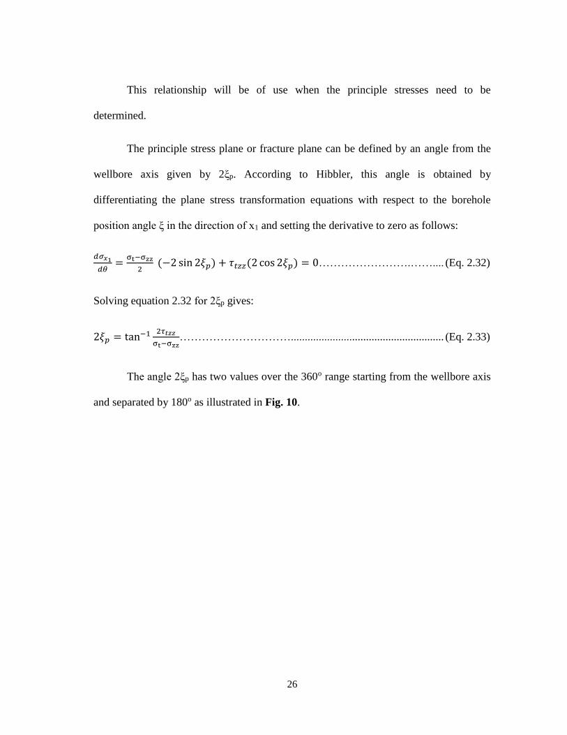
The principle stress plane or fracture plane can be defined by an angle from the
wellbore axis given by 2ξp According to Hibbler this angle is obtained by
differentiating the plane stress transformation equations with respect to the borehole
position angle ξ in the direction of x1 and setting the derivative to zero as follows
1198891205901199091
119889120579=
σtminusσzz
2 (minus2 sin 2120585119901) + 120591119905119911119911(2 cos 2120585119901) = 0helliphelliphelliphelliphelliphelliphelliphelliphelliphellip (Eq 232)
Solving equation 232 for 2ξp gives
2120585119901 = tanminus1 2120591119905119911119911
σtminusσzzhelliphelliphelliphelliphelliphelliphelliphelliphelliphellip (Eq 233)
The angle 2ξp has two values over the 360o range starting from the wellbore axis
and separated by 180o as illustrated in Fig 10
27
Fig 10 - Illustration of the resulting principle stresses acting on the plane of zero
shears containing the induced fractures
Now that the principle or fracture plane has been clearly defined the principle
stresses acting directly on this plane can be determined To determine these stresses
simple geometry in relation to the principle plane angle is applied according to Fig 11
Wellbore Section Axis Plane of zero shear
(Principle or Fracture Plane)
2ξp
σ1
σ2
28
Fig 11 - The geometry used to derive the equation for the principle stresses acting
directly on the fracture plane
Using Pythagoreanrsquos theorem and simple geometry the first principle stress is
determined by substituting the principle angle in the plane stress transformation
equation 228 in the direction of x1 (σx1) as follows
H2 = (2τtzz)2 + (σt minus σzz)2helliphelliphelliphelliphelliphelliphelliphelliphelliphellip (Eq 234)
σ1 =σt+σzz
2+
σtminusσzz
2 cos 2ξp + τtzz sin 2ξphelliphelliphelliphelliphelliphelliphelliphellip (Eq 235)
Substituting the parameters described in Fig 11 in this equation yields
σ1 =σt+σzz
2+
σtminusσzz
2 (
σtminusσzz
H) + τtzz(
2τtzz
H) helliphelliphelliphelliphelliphelliphelliphelliphellip (Eq 236)
Substituting the value for the hypotenuse (H) yields the following equation
σ1 =σt+σzz
2+
σtminusσzz
2 (
σtminusσzz
(2τtzz)2+(σtminusσzz)2) + τtzz(
2τtzz
(2τtzz)2+(σtminusσzz)2)helliphelliphelliphellip (Eq 237)
Rearranging the terms results in the next expression
2ξp
2τtzz
σt - σzz
H
sin 2120585119901 =2120591119905119911119911
H
cos 2120585119901 =σt minus σzz
119867
29
σ1 =σt+σzz
2+ radic(
σtminusσzz
2)2 minus τtzz
2helliphelliphelliphelliphelliphelliphelliphelliphelliphelliphelliphelliphelliphelliphelliphelliphellip (Eq 238)
This is the expression for the maximum wellbore principle plane stress acting
perpendicular to the fracture plane as described in Fig 10 To determine the second
principle stress the relationship between transformed plane stresses in both directions
(x1 and y1) and the pretransformed stresses must be recalled (Eq 231) The same
relationship applies to wellbore principle plane stresses ie the sum of the wellbore
principle plane stresses is equal to the sum of the pretransformed stresses (σt and σzz) and
expressed as follows
σ1 + σ2 = σt + σzzhelliphelliphelliphelliphelliphelliphelliphelliphelliphelliphelliphelliphelliphelliphelliphelliphelliphelliphelliphelliphelliphellip (Eq 239)
Therefore the following two equations follow
σ2 = σt + σzz minus σ1helliphelliphelliphelliphelliphelliphelliphelliphelliphelliphelliphelliphelliphelliphelliphelliphelliphelliphelliphelliphellip(Eq 240)
σ2 =σt+σzz
2minus radic(
σtminusσzz
2)2 minus τtzz
2helliphelliphelliphelliphelliphelliphelliphelliphelliphelliphelliphelliphelliphelliphelliphelliphellip(Eq 241)
Eq 241 is the expression for the minimum wellbore principle plane stress acting
parallel to the fracture on the fracture plane as described in Fig 10
In many references the expression for the maximum wellbore principle plane
stress (σ1) is denoted as the ldquomaximum tensile stressrdquo (Amadei 1997b Watson et al
2003) The reason for this denotation is that the maximum wellbore principle plane
stress is the deciding factor in the process of determining the initial fracture-pressure
gradient which means that the applied pressure must exceed this value for the fracture to
30
initiate However a complication arises from the fact that this principle stress changes
value around the circumference of the borehole This complication means that the model
cannot advance until a critical value of the maximum wellbore principle plane stress is
defined
The role of the model is to determine the location of the borehole wall where the
maximum wellbore principle plane stress is at its minimum value Determining the
location of this critical value requires that the model run the calculations at all points
around the borehole circumference until the minimum value is determined Then this
borehole location is denoted as the critical borehole position angle (θc) as illustrated in
Fig 12 The model will then run the calculation at this critical angle with ascending
values of the wellbore pressure The purpose of this step is to determine the value of the
wellbore pressure sufficient to reduce the maximum wellbore principle plane stress to
zero which means that the wellbore pressure exerted by the drilling fluid has exceeded
the maximum tensile stress of the formation Therefore the fracture will be initiated and
the value of the targeted fracture pressure is equal to the wellbore pressure that was
capable of reducing the maximum tensile stress to zero
31
Fig 12 - The location of the critical angle θc
The concept of plane stress transformation used here is for 2D situations hence
the transformation produces only two wellbore principle plane stresses For the purpose
of consistency and to comply with the 3D model a third principle stress needs to be
defined This stress is the equivalent of the radial stress defined in equation 215 Thus
the third principal stress is given by
σ3 = σr = Pwhelliphelliphelliphelliphelliphelliphelliphelliphelliphelliphelliphelliphelliphelliphelliphelliphelliphelliphelliphelliphelliphelliphelliphelliphellip(Eq 242)
25 Model Assumptions and the Corresponding Implications and Corrections
The model is based on the assumptions that include
32
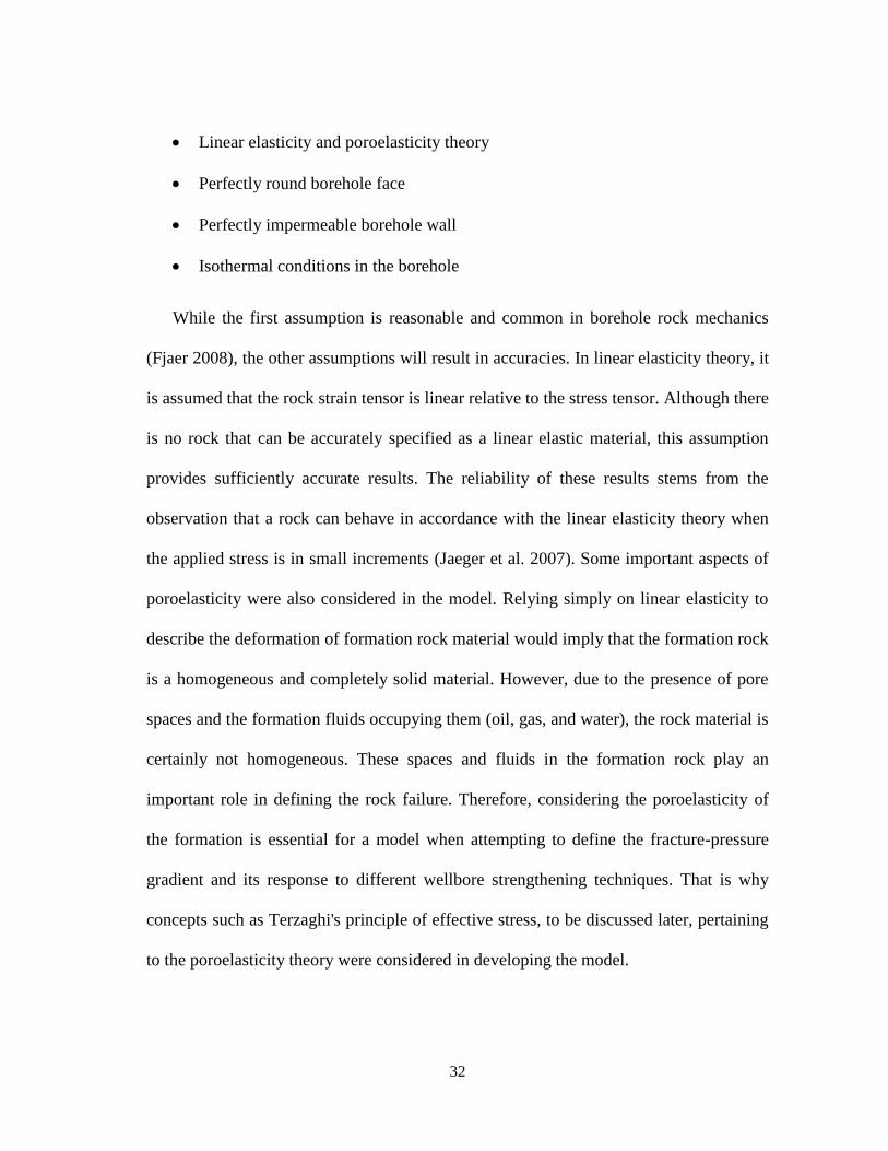
Linear elasticity and poroelasticity theory
Perfectly round borehole face
Perfectly impermeable borehole wall
Isothermal conditions in the borehole
While the first assumption is reasonable and common in borehole rock mechanics
(Fjaer 2008) the other assumptions will result in accuracies In linear elasticity theory it
is assumed that the rock strain tensor is linear relative to the stress tensor Although there
is no rock that can be accurately specified as a linear elastic material this assumption
provides sufficiently accurate results The reliability of these results stems from the
observation that a rock can behave in accordance with the linear elasticity theory when
the applied stress is in small increments (Jaeger et al 2007) Some important aspects of
poroelasticity were also considered in the model Relying simply on linear elasticity to
describe the deformation of formation rock material would imply that the formation rock
is a homogeneous and completely solid material However due to the presence of pore
spaces and the formation fluids occupying them (oil gas and water) the rock material is
certainly not homogeneous These spaces and fluids in the formation rock play an
important role in defining the rock failure Therefore considering the poroelasticity of
the formation is essential for a model when attempting to define the fracture-pressure
gradient and its response to different wellbore strengthening techniques That is why
concepts such as Terzaghis principle of effective stress to be discussed later pertaining
to the poroelasticity theory were considered in developing the model
33
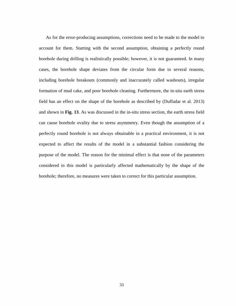
As for the error-producing assumptions corrections need to be made to the model to
account for them Starting with the second assumption obtaining a perfectly round
borehole during drilling is realistically possible however it is not guaranteed In many
cases the borehole shape deviates from the circular form due to several reasons
including borehole breakouts (commonly and inaccurately called washouts) irregular
formation of mud cake and poor borehole cleaning Furthermore the in-situ earth stress
field has an effect on the shape of the borehole as described by (Duffadar et al 2013)
and shown in Fig 13 As was discussed in the in-situ stress section the earth stress field
can cause borehole ovality due to stress asymmetry Even though the assumption of a
perfectly round borehole is not always obtainable in a practical environment it is not
expected to affect the results of the model in a substantial fashion considering the
purpose of the model The reason for the minimal effect is that none of the parameters
considered in this model is particularly affected mathematically by the shape of the
borehole therefore no measures were taken to correct for this particular assumption
34
Fig 13 - The effect of in-situ earth stress field on the shape of the borehole
(Duffadar et al 2013)
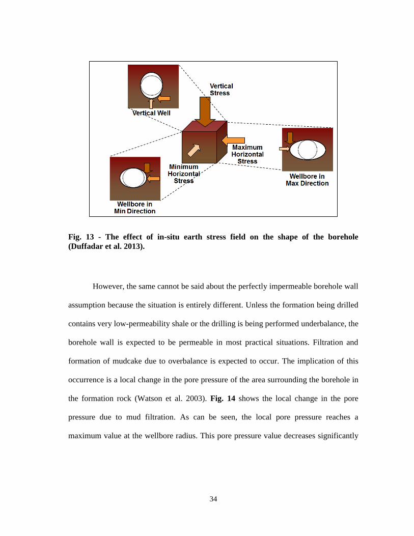
However the same cannot be said about the perfectly impermeable borehole wall
assumption because the situation is entirely different Unless the formation being drilled
contains very low-permeability shale or the drilling is being performed underbalance the
borehole wall is expected to be permeable in most practical situations Filtration and
formation of mudcake due to overbalance is expected to occur The implication of this
occurrence is a local change in the pore pressure of the area surrounding the borehole in
the formation rock (Watson et al 2003) Fig 14 shows the local change in the pore
pressure due to mud filtration As can be seen the local pore pressure reaches a
maximum value at the wellbore radius This pore pressure value decreases significantly
35
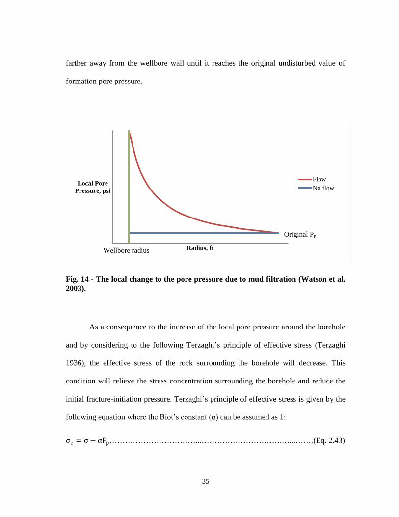
farther away from the wellbore wall until it reaches the original undisturbed value of
formation pore pressure
Fig 14 - The local change to the pore pressure due to mud filtration (Watson et al
2003)
As a consequence to the increase of the local pore pressure around the borehole
and by considering to the following Terzaghirsquos principle of effective stress (Terzaghi
1936) the effective stress of the rock surrounding the borehole will decrease This
condition will relieve the stress concentration surrounding the borehole and reduce the
initial fracture-initiation pressure Terzaghirsquos principle of effective stress is given by the
following equation where the Biotrsquos constant (α) can be assumed as 1
σe = σ minus αPphelliphelliphelliphelliphelliphelliphelliphelliphelliphelliphelliphelliphelliphelliphelliphelliphelliphelliphelliphelliphelliphelliphelliphellip (Eq 243)
Local Pore
Pressure psi
Radius ft
Flow
No flow
Original Pp
Wellbore radius
36
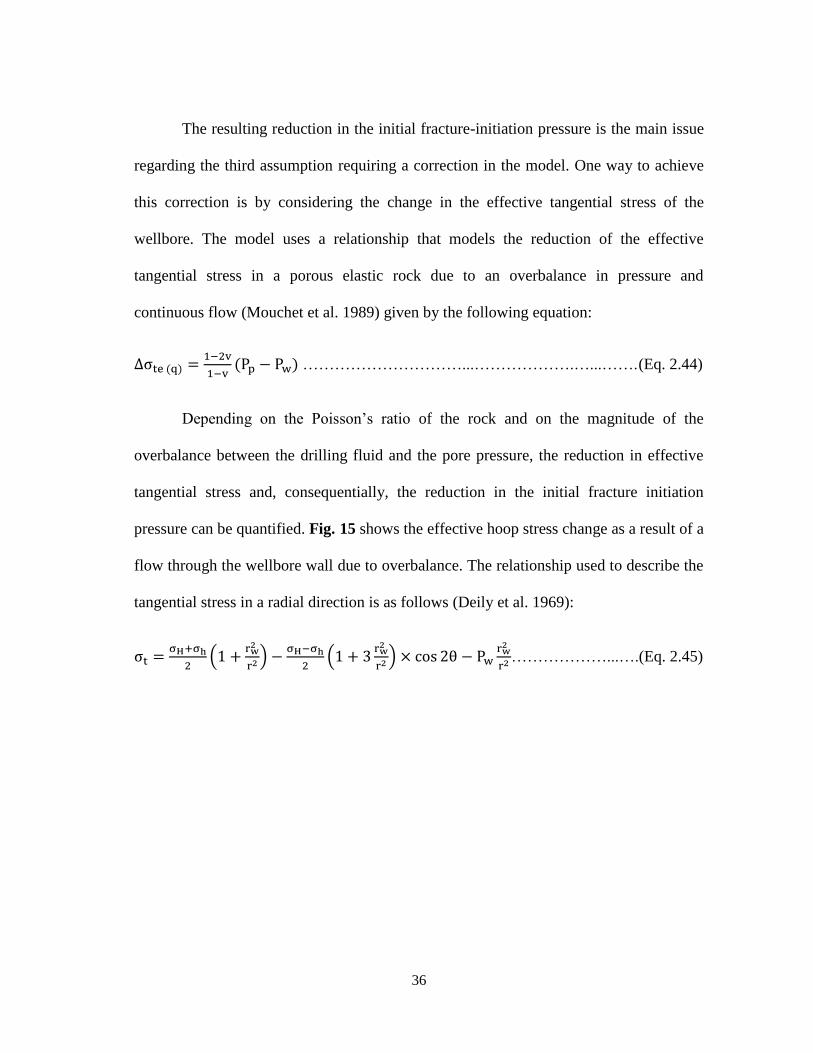
The resulting reduction in the initial fracture-initiation pressure is the main issue
regarding the third assumption requiring a correction in the model One way to achieve
this correction is by considering the change in the effective tangential stress of the
wellbore The model uses a relationship that models the reduction of the effective
tangential stress in a porous elastic rock due to an overbalance in pressure and
continuous flow (Mouchet et al 1989) given by the following equation
∆σte (q) =1minus2v
1minusv(Pp minus Pw) helliphelliphelliphelliphelliphelliphelliphelliphelliphelliphelliphelliphelliphelliphelliphelliphelliphelliphellip (Eq 244)
Depending on the Poissonrsquos ratio of the rock and on the magnitude of the
overbalance between the drilling fluid and the pore pressure the reduction in effective
tangential stress and consequentially the reduction in the initial fracture initiation
pressure can be quantified Fig 15 shows the effective hoop stress change as a result of a
flow through the wellbore wall due to overbalance The relationship used to describe the
tangential stress in a radial direction is as follows (Deily et al 1969)
σt =σH+σh
2(1 +
rw2
r2 ) minusσHminusσh
2(1 + 3
rw2
r2 ) times cos 2θ minus Pwrw
2
r2 helliphelliphelliphelliphelliphelliphellip(Eq 245)
37
Fig 15 - Illustration of the change undergone by the effective hoop stress as a result
of wellbore wall flow due to overbalance
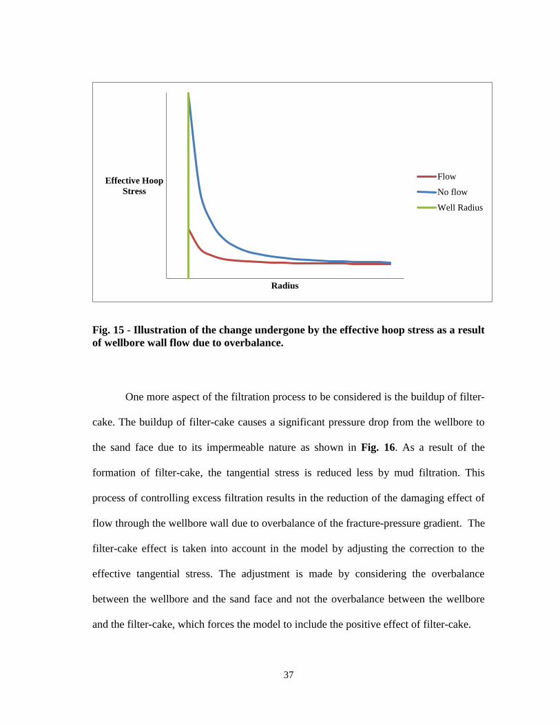
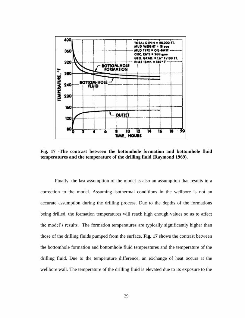
One more aspect of the filtration process to be considered is the buildup of filter-
cake The buildup of filter-cake causes a significant pressure drop from the wellbore to
the sand face due to its impermeable nature as shown in Fig 16 As a result of the
formation of filter-cake the tangential stress is reduced less by mud filtration This
process of controlling excess filtration results in the reduction of the damaging effect of
flow through the wellbore wall due to overbalance of the fracture-pressure gradient The
filter-cake effect is taken into account in the model by adjusting the correction to the
effective tangential stress The adjustment is made by considering the overbalance
between the wellbore and the sand face and not the overbalance between the wellbore
and the filter-cake which forces the model to include the positive effect of filter-cake
Effective Hoop
Stress
Radius
Flow
No flow
Well Radius
38
Fig 16 - Illustration of the effect of the buildup of filter-cake as a drop in pressure
from the wellbore to the sand face due to its impermeable nature
Local Pore
Pressure
Radius
With No Mud Cake
With Mud Cake
Wellbore
radius
Filter-cake
thickness
rw
Pw
With no filter-cake
With filter-cake
39
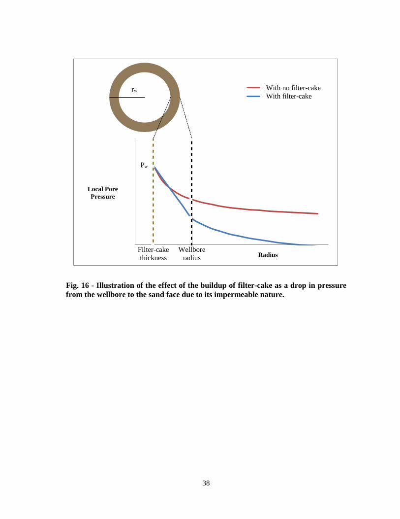
Fig 17 -The contrast between the bottomhole formation and bottomhole fluid
temperatures and the temperature of the drilling fluid (Raymond 1969)
Finally the last assumption of the model is also an assumption that results in a
correction to the model Assuming isothermal conditions in the wellbore is not an
accurate assumption during the drilling process Due to the depths of the formations
being drilled the formation temperatures will reach high enough values so as to affect
the modelrsquos results The formation temperatures are typically significantly higher than
those of the drilling fluids pumped from the surface Fig 17 shows the contrast between
the bottomhole formation and bottomhole fluid temperatures and the temperature of the
drilling fluid Due to the temperature difference an exchange of heat occurs at the
wellbore wall The temperature of the drilling fluid is elevated due to its exposure to the
40
formation rock and most importantly the formation rock temperature decreases due to
its exposure to the colder fluid The formation rock exposure to the lower temperature
can alter its stress state This change in the rock stress state is logical when considering
the physical effect a sudden temperature change can have on material such as rocks The
resulting physical expansion or contraction in the rock is the driving force behind the
change of the stress state In the case of deep wells where the geothermal gradient causes
the formation rock to be of higher in temperature than the drilling fluid the drilling fluid
will act to cool the formation rock with circulation time The result of this interaction
will be contraction of the formation rock over time due to cooling which will have a
detrimental effect on fracture-pressure gradient in the form of a decrease In the
opposite case of shallow wells or of high-temperature drilling fluid the colder formation
rock will absorb heat from the drilling fluid This will cause an expansion of the
formation rock volume and an increase in the fracture-pressure gradient
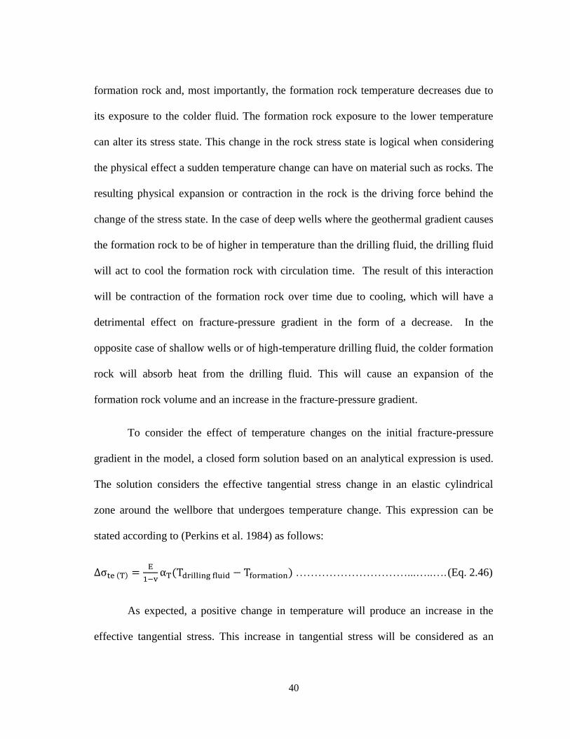
To consider the effect of temperature changes on the initial fracture-pressure
gradient in the model a closed form solution based on an analytical expression is used
The solution considers the effective tangential stress change in an elastic cylindrical
zone around the wellbore that undergoes temperature change This expression can be
stated according to (Perkins et al 1984) as follows
∆σte (T) =E
1minusvαT(Tdrilling fluid minus Tformation) helliphelliphelliphelliphelliphelliphelliphelliphelliphelliphelliphellip (Eq 246)
As expected a positive change in temperature will produce an increase in the
effective tangential stress This increase in tangential stress will be considered as an
41
incremental gain to the total fracture-pressure gradient in the model Likewise a
negative change in temperature will decrease the effective tangential stress This
reduction of the tangential stress will be considered a reduction in the total fracture-
pressure gradient in the model
26 The Evaluation of Fracture-Pressure Gradient Enhancement
Due to the continuous maturation and depletion of reservoirs worldwide the
drilling window is narrowing significantly in many fields The reduction in the drilling
window can be attributed to falling pore pressures and the consequent decrease in the
minimum horizontal in-situ stress as described by this relationship
σH =v
1minusv(σV minus Pp) + Pp helliphelliphelliphelliphelliphelliphelliphelliphelliphelliphelliphelliphelliphelliphelliphelliphelliphelliphellip(Eq 247)
42
Fig 18 - The resulting narrower drilling window due to reservoir depletion
The decrease in the minimum horizontal stress leads to a reduction in the
fracture-pressure gradient The resulting narrower drilling window as described in Fig
18 presents various challenges to drilling operations A drilling fluid can typically be
designed to accommodate both the fracture gradient and the pore pressure gradient in
static conditions However in dynamic conditions where the equivalent circulation
density is higher than the static mud weight due to annual friction pressure the fracture
gradient can easily be exceeded resulting in lost circulation Plus there is no guarantee
that such a drilling fluid which was designed for the restriction condition of the narrow
Dep
th
ft
Pressure psi
Fracture Pressure
Pore Pressure
New Pore Pressure Gradient
New Fracture Pressure Gradient
Narrowing down of drilling
window due to depletion
43
drilling window can provide wellbore stability One tool which can give a wider drilling
window is wellbore strengthening techniques
Over the years various wellbore strengthening techniques were developed to
increase the fracture-pressure gradient and widen the drilling window The benefits of
these techniques could also include the elimination of lost circulation and sand
production The wellbore strengthening techniques can be classified according to the
type of their interaction with targeted formation rock as follows (Barrett et al 2010)
1 Physical methodsmdashreduce the fluid rock interaction by means of plastering
2 Chemical methodsmdashchemical grouting dictating the dynamics of the formation
fluid through osmotic mechanisms and using deformable viscous and cohesive
systems (DVC)
3 Thermal methodsmdashincrease the temperature of the rock in the wellbore wall
through heat transfer from the drilling fluid to cause rock expansion and an
increase in the tangential stress
4 Mechanical methodsmdashenhance the tangential stress of the wellbore by inducing
fractures and plugging or sealing them in what is known as ldquostress cagingrdquo
(Aston et al 2004)
The focus of this work will be on techniques that deal directly with rock stresses as
the driving force for enhancing the fracture-pressure gradient Those techniques include
the wellbore strengthening techniques that stabilize the rocks existing or induced
fractures either by plugging or sealing to change the stress state around the wellbore
44
They also include the techniques that use wellbore temperature variations to alter the
stress around the wellbore
261 Evaluation of Wellbore Strengthening Techniques from Basic Rock Mechanics
The model requires a mathematical representation of the induced stress alteration
due to the action of the different wellbore strengthening techniques Building the model
on an analytical or exact solution would be the ideal case however there is no such
solution available where the stress state alteration is quantified due to the effects of
different wellbore strengthening techniques as reported in the literature Therefore the
model relies on an approximate solution to achieve this This solution was developed by
Nobuo Morita (Morita et al 2012) as a closed-form solution based on a boundary
element model According to Moritarsquos laboratory work the model accuracy in its
different variations ranges from 02 to 5 hence it was deemed suitable for the
purpose of the model being developed for this work
The main advantage of the selected solution is that it relies on basic rock
mechanics principles to determine the enhancement to the fracture-pressure gradient
These basic rock mechanics principles make the solution more accessible from an
operation point of view The data used to describe these principles are easily obtainable
through the cooperation of the drilling engineer and the field geologist Also this
solution is particularly useful for the purpose of the model being constructed by applying
it to actual field data Moritarsquos approach to addressing the evaluation of wellbore
45
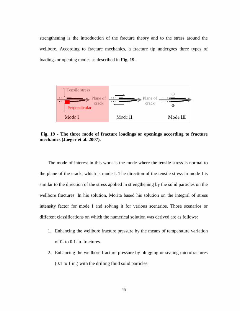
strengthening is the introduction of the fracture theory and to the stress around the
wellbore According to fracture mechanics a fracture tip undergoes three types of
loadings or opening modes as described in Fig 19
Fig 19 - The three mode of fracture loadings or openings according to fracture
mechanics (Jaeger et al 2007)
The mode of interest in this work is the mode where the tensile stress is normal to
the plane of the crack which is mode I The direction of the tensile stress in mode I is
similar to the direction of the stress applied in strengthening by the solid particles on the
wellbore fractures In his solution Morita based his solution on the integral of stress
intensity factor for mode I and solving it for various scenarios Those scenarios or
different classifications on which the numerical solution was derived are as follows
1 Enhancing the wellbore fracture pressure by the means of temperature variation
of 0- to 01-in fractures
2 Enhancing the wellbore fracture pressure by plugging or sealing microfractures
(01 to 1 in) with the drilling fluid solid particles
Plane of
crack
Plane of
crack
Tensile stress
Perpendicular
46
3 Enhancing the wellbore fracture pressure by plugging or sealing macrofractures
(1 to 2 ft) with the drilling fluid solid particles in what is known as the stress
cage method
4 Enhancing the wellbore fracture pressure by plugging or sealing large fractures
(more than 10 ft) with the drilling fluid solid particles in what is known as the tip
screening method
Based on those scenarios mathematical relationships of fracture-pressure
enhancement were derived These relationships were added to the model to quantify the
change to the initial virgin fracture-pressure gradient in a specific section of the well
when different wellbore strengthening techniques are implemented
The first scenario of wellbore strengthening in the model deals with the resultant
fracture-pressure enhancement when a naturally existing or induced microfacture is
purposely sealed at the fracture mouth by solid particles from a ldquodesigner mudrdquo This
scenario can be considered as a branch of the ldquostress cagerdquo method In the ldquostress cagerdquo
method an induced fracture is created and kept open by solid particles from a ldquodesigner
mudrdquo for the purpose of increasing the hoop stress of the wellbore Field applications
showed that applying this method does indeed enhance the fracture pressure in the
wellbore section where it is applied (Aston et al 2004) However there is no clear
physical evidence of what the nature of the interaction between the solid particles from
the ldquodesigner mudrdquo and the induced fracture actually is For this reason the model takes
into account these different scenarios to examine this particular wellbore strengthening
technique For the purpose of the model this scenario of fracture and solid particle
47
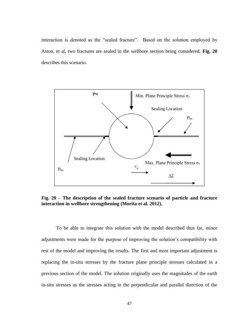
interaction is denoted as the ldquosealed fracturerdquo Based on the solution employed by
Aston et al two fractures are sealed in the wellbore section being considered Fig 20
describes this scenario
Fig 20 ndash The description of the sealed fracture scenario of particle and fracture
interaction in wellbore strengthening (Morita et al 2012)
To be able to integrate this solution with the model described thus far minor
adjustments were made for the purpose of improving the solutionrsquos compatibility with
rest of the model and improving the results The first and most important adjustment is
replacing the in-situ stresses by the fracture plane principle stresses calculated in a
previous section of the model The solution originally uses the magnitudes of the earth
in-situ stresses as the stresses acting in the perpendicular and parallel direction of the
Sealing Location
Sealing Location Max Plane Principle Stress σ1
Min Plane Principle Stress σ2
Pbu
Pbu
48
fractures The model seeks to improve the use of this particular aspect of the solution by
considering the principle stresses acting on the specific plane of the fractures (the plane
of zero shear) as the stresses acting in the perpendicular and parallel direction of the
fractures As such the model will take the magnitude of these stresses in the solution
instead of the magnitude of the earth in-situ stresses which means that the minimum
fracture plane principle stress will act in the perpendicular direction to the fracture and
prevent its propagation
The second change to the solution is made for the sole purpose of its
compatibility with the rest of the model In the original solution the signs for the stresses
were assigned as positive for tension and negative for compression This sign assignment
will not work with the rest of the model Nevertheless all of the stresses being
considered in all of the previous sections of the model were compressive thus the
solution was adjusted so that all of the stresses used will be a positive value for
compression
In Fig 20 describing this first scenario of wellbore strengthening Pbu is the
pressure inside of the fracture or the buildup pressure This value will be equal to the
pore pressure in the majority of cases The reason for this condition is that one of the
main requirements for applying the ldquostress cagerdquo method is high-rock permeability The
high permeability is required because it will allow the ldquodesigner mudrdquo filtrate to flow
into the formation and prevent further and unwanted fracture propagation Therefore the
high permeability will aid in arresting the fracture growth to a desired length and will
dissipate the pressure inside of the fracture until it reaches the original pore pressure of
49
the rock In the less probable case of a low-permeability rock the filtrate is expected to
create a pressure buildup in the fracture The result would be a higher pressure inside of
the fracture than the original pore pressure of the rock
After making the required adjustments to the solution the final equation for the
enhanced fracturing pressure for the first scenario that will be used in the model will be
as follows
119875119891minus119890119899ℎ119886119899119888119890119889 =
119896119888
radic120587∆119871+1205902119865120582(119904)minus119875119887119906[1+(1minus119904)(minus0137+0258(1minus119904)2minus041199042(1minus119904))]
(1minus119904)[0637+0485(1minus119904)2+041199042(1minus119904)helliphelliphellip(Eq 248)
Where
∆119871 =119882119888119864
4(1minus1199072)(1205902minus119875119887119906)helliphelliphelliphelliphelliphelliphelliphelliphelliphelliphelliphelliphelliphelliphelliphelliphelliphelliphelliphelliphelliphellip( Eq 249)
120582 =1205901
1205902helliphelliphelliphelliphelliphelliphelliphelliphelliphelliphelliphelliphelliphelliphelliphelliphelliphelliphelliphelliphelliphelliphelliphelliphelliphelliphellip( Eq 250)
119904 =∆119871
(119903119908+∆119871)helliphelliphelliphelliphelliphelliphelliphelliphelliphelliphelliphelliphelliphelliphelliphelliphelliphelliphelliphelliphelliphelliphelliphelliphellip( Eq 251)
120596 =119875119887119906
1205902helliphelliphelliphelliphelliphelliphelliphelliphelliphelliphelliphelliphelliphelliphelliphelliphelliphelliphelliphelliphelliphelliphelliphelliphelliphellip( Eq 252)
1198651(119904) = 1 + (1 minus 119904)[05 + 0743(1 minus 119904)2]helliphelliphelliphelliphelliphelliphelliphelliphelliphelliphelliphellip( Eq 253)
119865119900(119904) = 05(3 minus 119904)[1 + 1243(1 minus 119904)3] helliphelliphelliphelliphelliphelliphelliphelliphelliphelliphelliphelliphellip( Eq 254)
119865120582(119904) = (1 minus 120582)119865119900(119904) + 1205821198651(119904)helliphelliphelliphelliphelliphelliphelliphelliphelliphelliphelliphelliphelliphelliphelliphellip( Eq 255)
The second scenario considers a different type of solid particle and fracture
interaction Instead of assuming that the solid particles from the ldquodesigner mudrdquo seal the
50
fracture at the fracture mouth it assumes that the particles are plugging the fracture at a
certain distance from the fracture mouth Again due to the ambiguity in the nature of the
interaction between the fracture and the designer mud solid particles this scenario can
be considered as a branch of the ldquostress cagerdquo method This scenario is denoted as the
plugged fracture technique in the model as opposed to the sealed fracture techniques
discussed previously The closed-from solution used in the model for the plugged
fracture scenario is similar to the sealed-fracture scenario in that it also considers two
fractures created in the wellbore section being considered as shown in Fig 21
Fig 21 - The description of the plugged fracture scenario of particle and fracture
interaction in wellbore strengthening (Morita et al 2012)
Min Plane Principle Stress σ2
Max Plane Principle
Stress σ1
Pbu
Pbu
51
The same changes that were applied to the sealed-fracture scenario solution were
also applied to the plugged-fracture solution to ensure its compatibility with the rest of
the model and to achieve the desired improvements However there are some notable
differences between the descriptions of the two scenarios In this scenario the parameter
ldquoardquo defines the distance at which the solid particles plug the fracture and the parameter
ΔL defines the length of the fracture excluding the plugging distance In the sealed-
fracture scenario ΔL defines the length of the fracture as a whole Also the solution
considers the pressure buildup Pbu to be in effect behind the plugging particles only
After making the required adjustments to the solution the final equation for the
enhanced fracturing pressure for the second scenario that will be used in the model will
be as follows
119875119891minus119890119899ℎ119886119899119888119890119889 =
119896119888
radic120587(119886+∆119871)+1205902119865120582(119904)minus2119871
119875119887119906
radic120587(119886+∆119871)radic120587119871[119886119903119888119904119894119899radic
∆119871
2119871minus119886119903119888119904119894119899radic
2119871minus∆119871
2119871+
120587
2]
1+(1minus119904)(05+0743(1minus119904)2)minus21198711
radic120587(119886+∆119871)radic120587119871[119886119903119888119904119894119899radic
∆119871
2119871minus119886119903119888119904119894119899radic
2119871minus∆119871
2119871+
120587
2]
(Eq 256)
Where
∆119871 =119882119888119864
4(1minus1199072)(1205902minus119875119887119906)helliphelliphelliphelliphelliphelliphelliphelliphelliphelliphelliphelliphelliphelliphelliphelliphelliphelliphelliphelliphellip( Eq 257)
120582 =1205901
1205902helliphelliphelliphelliphelliphelliphelliphelliphelliphelliphelliphelliphelliphelliphelliphelliphelliphelliphelliphelliphelliphelliphelliphelliphelliphellip( Eq 258)
119904 =119886+∆119871
(119903119908+119886+∆119871)helliphelliphelliphelliphelliphelliphelliphelliphelliphelliphelliphelliphelliphelliphelliphelliphelliphelliphelliphelliphelliphelliphellip( Eq 259)
119871 = 119903119908 + 119886 + ∆119871helliphelliphelliphelliphelliphelliphelliphelliphelliphelliphelliphelliphelliphelliphelliphelliphelliphelliphelliphelliphelliphellip( Eq 260)
52
120596 =119875119887119906
1205902helliphelliphelliphelliphelliphelliphelliphelliphelliphelliphelliphelliphelliphelliphelliphelliphelliphelliphelliphelliphelliphelliphellip( Eq 261)
1198651(119904) = 1 + (1 minus 119904)[05 + 0743(1 minus 119904)2] helliphelliphelliphelliphelliphelliphelliphelliphelliphelliphellip( Eq 262)
119865119900(119904) = 05(3 minus 119904)[1 + 1243(1 minus 119904)3] helliphelliphelliphelliphelliphelliphelliphelliphelliphelliphelliphelliphellip( Eq 263)
119865120582(119904) = (1 minus 120582)119865119900(119904) + 1205821198651(119904)helliphelliphelliphelliphelliphelliphelliphelliphelliphelliphelliphelliphelliphelliphelliphelliphellip( Eq 264)
27 Model Interface
For the purpose of generating results in a timely manner a user-friendly interface
was created to accompany the models VBA Excel programming code The interface
accepts the input data from the user that defines the section of the well being targeted for
examination field stress data rock basic mechanical properties and wellbore
strengthening techniques data The initial results of the model can be obtained using the
command buttons shown in Fig 22
53
Fig 22 - The command buttons used in the model to obtain the initial results
These command buttons perform the initial calculations of the model and display the
results in the form of a message box and on an Excel spreadsheet The commands
performed are as follows
1 Display the value of the critical angle (θc) which defines the circumferential position
of fracture initiation in the wellbore wall
2 Display the full calculations performed at every degree of the wellbore
circumference
3 Display the value of the initial fracture gradient (gfi) corresponding to the section of
the well being examined
4 Display the angle of the zero shear plane (2ξp)
54
5 Display the correction to the effective tangential stress due to mud filtration (Δσte(q))
and temperature change (Δσte(T))
6 Display the user form that enables generating parametric analysis of the effect of
various parameters on the initial fracture-pressure gradient and the temperature- and
mud filtrate-affected fracture-pressure gradients
7 Display the user form that enables the user to enter the data required for each
wellbore strengthening scenario
8 Display the user form that enables the user to generate the ease-of-drilling polar
plots
The model requires specific input data to perform the wellbore strengthening
evaluation calculations The first input is selecting the type or the scenario of solid
particles and fracture interaction After pressing the ldquoParticle Fracture Interaction in WS
Techrdquo the user form shown in Fig 23 will appear
55
Fig 23 - The user form that enables the model to select the particle and fracture
interaction scenario and input the data for each scenario
The user can select the appropriate scenario and enter the required data that can
be related to the closed-form solution as follows
1 Wellbore radius (rw) in inches
2 Fracture aperture (Wc) in inches
3 Fracture toughness (kc) in psiinch12
56
4 Fracture-pressure buildup (Pub) in psi if left blank assumed to be zero
5 Plug placement distance from the mouth of the fracture (a) in inches (applies to the
plugged fracture option only)
This will enable obtaining the fracture-pressure gradient resulting from applying the
selected wellbore strengthening technique
The ldquoParametric Analysisrdquo command button shown in Fig 22 will prompt the form
shown in Fig 24
Fig 24 - The user form that enables selecting the base variable for the initial
parametric analysis
57
This user form produces different plots that show the effect of the four
parameters listed on
1 The initial fracture-pressure gradient (gfi)
2 The temperature-influenced fracture-pressure gradient (gfi(T))
3 The mud filtrate-influenced fracture-pressure gradient (gfi(q))
4 The combined temperature and mud filtrate- influenced fracture-pressure gradient
(gfi(qT))
The user form allows for entering a value for a parameter that will be the base
for the parametric analysis This input value will be used as the center of a range of
values of the particular parameter Then the code will calculate the different types of
the fracture-pressure gradient at each value of the parameter and will plot the results
graphically in a separate Excel worksheet
A similar analysis can be performed on the wellbore strengthening influenced
fracture-pressure gradient using the form shown in Fig 25
58
Fig 25 - The user form that enables selecting the base variable for the final
parametric analysis
This form can be obtained by pressing the command button ldquoParametric
Analysisrdquo in the user form shown in Fig 23 and it performs the same task as the user
form shown in Fig 24 The only difference is that this form offers more parameters to be
used as the basis of the analysis These additional parameters are concerned with the
59
solid particle and fracture interaction type The produced plots will show the trend
exhibited by the following
1 Initial fracture-pressure gradient gfi
2 Wellbore strengthening influenced fracture-pressure gradient gfFS
3 Temperature and wellbore strengthening influenced fracture-pressure gradient gfFS(T)
4 Mud filtrate and wellbore strengthening influenced fracture-pressure gradient gfFS(q)
5 Temperature mud filtrated and wellbore strengthening combined influenced
fracture-pressure gradient gfFS(qT)
For the purpose of analyzing the performance of wellbore strengthening techniques
based on the well section placement with respect to the field in-situ stresses the options
shown in Fig 26 were created
60
Fig 26 - Ease of drilling data user form
The user form shown in Fig 26 will be used to create polar plots that show the
ease of drilling that particular section of the well based on the well surface location and
trajectory The generated plots use the well azimuth angle in polar coordinates to display
all of the possible well placement scenarios In radial coordinates a parameter that can
be called ldquoease-of-drilling fractionrdquo is calculated and plotted for every possible well
placement scenario The purpose of this parameter is to demonstrate the size of the
drilling window compared with a reference window size The code uses two references
for the drilling window size when calculating the ease-of-drilling fraction The first
reference is based on the maximum possible fracture-pressure gradient in the 360o
azimuth range for the individual well section and fracture-pressure gradient type in
61
consideration Based on this fracture-pressure gradient the ease-of-drilling fraction will
be calculated for each 05o of the 360o azimuth as follows
Ease of Drilling Fraction (Based on Maximum gf) =gf
Max gfhelliphelliphelliphelliphelliphelliphellip(Eq 265)
This calculation is done for all of the different types of fracture-pressure
gradients which include the initial fracture-pressure gradient gfi the temperature-
influenced fracture-pressure gradient gf(T) the mud filtrate-influenced fracture-pressure
gradient gf(q) and the temperature and mud filtrate combined influenced fracture-
pressure gradient gf(qT) Because the ease-of-drilling polar plot is based on a specific
and unique to the plot reference value (the maximum possible fracture-pressure gradient
in the 360o azimuth range) two different polar plots cannot be compared to each other to
decide which type of fracture-pressure gradient provides the wider drilling window in a
certain direction For that reason the code calculates the ease-of-drilling fraction with a
constant reference value for all the different types of fracture-pressure gradients as
follows
Ease of Drilling Fraction (Based on C psift) =gf
C helliphelliphelliphelliphelliphelliphelliphelliphelliphellip(Eq 266)
The reference value for the ease-of-drilling-fraction is selected to be equal to or
greater than the maximum possible value of the fracture-pressure gradient This
assumption will make it possible to compare different ease-of-drilling polar plots even if
they are based on different types of fracture-pressure gradients For example using the
constant reference in the ease-of-drilling fraction the ease-of-drilling polar plot for a
particular section of the well based on the initial fracture-pressure gradient can be
62
compared to the ease-of-drilling polar plot for the same section of the well based on the
wellbore strengthening influenced fracture-pressure gradient
Fig 27 shows a sample of the produced polar plots that will be discussed in more
details in the next chapter
Fig 27 - Samples of the produced polar plots highlighting the differences between
them each type
Non-Comparable
Comparable
63
3 MODEL RESULTS AND ANALYSIS (CASE STUDY SCENARIO)
31 The Case Study Setup
For the model to produce the targeted results there is a set of input data required
The input data is aimed at defining the following
The targeted wellbore section in terms of its position with respect to the field in-
situ stresses trajectory and depth
The field in-situ stresses in terms of magnitude and direction
The targeted formation pore pressure
The targeted formation basic rock mechanic parameters including Poissonrsquos
ratio Youngrsquos modulus and the thermal expansion coefficient
The drilling fluid properties including the pressure overbalance it provides and
the temperature change it brings to the wellbore
For the purpose of evaluating the general performance of the formation strengthening
techniques previously presented a case study is created based on typical and common
input parameter values The modelrsquos code accepts the input values and yields realistic
values as long as the input values for each parameter are within a reasonable range
Table 1 shows the values selected for this particular case study
64
Table 1 - The initial input values for the model case study
Input Depth ft 14000
Input Pore Pressure Gradient ppg 12
Input vertical Stress σv Gradient psift 0972
Input Poissons ratio ν 025
Input σH (max horiz) Gradient psift 08
Input σh (min horiz) Gradient psift 0739
Input Well Azimuth degree 88
Input Well inclination γ (Between σ1 and Borhole Axis) degree 70
Input σH (max horiz) direction measured from the north clock-wise degree
138
Input Beta β (Between σH and Borehole Projection on σH-σh Plane or Azimuth) degree
50
Input Actual Borehole Pressure Gradient for Δσte(q) Calculations ppg 121
Input Temperature Increment ΔT Fo 10
Input Youngs Modulus E psi 2500000
Input Coefficient of Thermal Expansion αT in(in -Fo) 0000008
These values represent typical values for a Gulf of Mexico field showing in-situ
stress anisotropy due to a salt dome intrusion (Watson et al 2003) In this case study the
vertical stress or the vertical overburden is the maximum in-situ stress however the
well section being considered is drilled with a 70o inclination angle In the model this
inclination angle is interpreted as a 70o deviation of the wellbore section from the
maximum in-situ stress direction Also the wellbore projection on the σH-σh plane is
located at 50o from the direction of the maximum horizontal stress σH all of which means that
the wellbore section does not fall on the same coordinate system as do the in-situ
stresses This condition will necessitate that the model performs the discussed
transformation of the in-situ stresses to the wellbore section coordinate system Fig 28
65
shows the visual representation of the position of the well section of interest with respect
to the in-situ stresses and the two coordinate systems involved in the transformation
process of the model
Fig 28 - Description of the case study well trajectory and position with respect to
the in-situ stresses (Watson et al 2003)
Upon performing the transformation the modelrsquos code will move to the
calculation of the induced stresses around the wellbore and eventually determine the two
principle stresses acting on the plane of zero shear stress The next step in the process is
Wellbore Direction Vector C
σv
σH=11200 psi σh=10346 psi
Wellbore Inclination Angle
θ Wellbore Position Angle
z
x y zrsquo
yrsquo xrsquo
70o
50o
66
determining the critical angle of the circumferential position of the wellbore which is
defined by the minimum value of the minimum principle stress The final step that the
model performs at this stage is defining the minimum wellbore pressure that has the
ability to set the effective minimum principle stress to zero This value of wellbore
pressure will be considered as the initial fracture pressure of formation
32 The Preliminary Results
In preparation for evaluating the wellbore strengthening techniques the model
produces the preliminary results as shown in Table 2 These values explain the fracture
system in the wellbore before applying any wellbore strengthening procedure The
values also depict the initial reaction of the fracture system to a wellbore pressure
overbalance resulting in mud filtration and to the wellbore wall exposure to drilling
fluid resulting in a change in the temperature The most important value in the
preliminary results is the initial fracture-pressure gradient This is the value that is going
to be used as a reference when the model reaches the wellbore strengthening techniques
evaluation portion and the well placement and trajectory evaluation portion
67
Table 2 - The model preliminary results
Critical Borehole Position Degrees 169
Fracture Initiation Gradient Δgfi psift 06957
Incremental Change in Effective Tangential Stress due to Flow Δσte(q) psig -485
Recalculated Fracture Initiation Gradient due to Flow Δgf(q) psift 06922
Incremental Change in Effective Tangential Stress due to Temperature Δσte(T) psig
2667
Recalculated Fracture Initiation Gradient due to Temperature Δgf(T) psift 07148
Recalculated Fracture Initiation Gradient due to Flow and Temperature Δgf(qT) psift
07113
Fracture Plane Angel Measured from the Wellbore Axis 2ξp Degrees -676
By examining the preliminary results the detrimental effect of the mud filtration
flow in the formation on the fracture-pressure gradient is clearly obvious As previously
discussed the reduction of the fracture-pressure gradient is the result of applying the
Biotrsquos principle of effective stress This fracture-pressure gradient reduction was built
into the model by introducing the overbalance and filtration correction relationship
discussed in Section 25 The beneficial effect of increasing the temperature of the
wellbore wall on the fracture-pressure gradient is also obvious The temperature effect
found in the model by introducing the temperature change correction relationship
discussed in Section 25
The model set up the transition to the wellbore strengthening techniques
evaluation by defining the plane of the fracture or the plane of zero shear stress The
plane of the fracture is defined by an angle measured from the wellbore section axis
Even though this angle has two values only one value is displayed because the two
values are separated by 180o and define the same plane The principle stress calculations
68
are performed in this stage of the model The model analyzes these calculations and
defines the value of the two principle stresses acting on the plane of zero shear stress at
the defined critical angle These are the stresses that will be used in evaluating the
wellbore strengthening techniquesrsquo performance
33 Wellbore Strengthening Evaluation Data and Preliminary Results
Additional input data are required for the evaluation These data describe the
nature of the interaction between the drilling fluid solid particles intended to be used for
the treatment and the initiated fractures A drilling engineer is not expected to have a
sufficient knowledge or access to this type data Therefore cooperation between a
drilling engineer a field geologist and a rock mechanics lab technician is required
Starting with the fracture aperture parameter it can be estimated based on the applied
stress as discussed in (Kulatilake et al 2006) As for the fracture toughness it can be
assigned a value based on the type of rock being treated Zhao et al and Senseny et al
discuss the process of fracture toughness determination and list typical values for the
parameter based on the rock type (Zhao et al 1993) (Senseny et al 1984) The plug
placement is determined based on the size of the drilling fluid bridging particle which
should be obtainable by the drilling engineer and the fracture aperture Finally pressure
buildup behind the plug can be estimated based on the permeability of the formation
rock As the rock permeability increases as the value of the pressure buildup approaches
69
zero It is preferable as will be discussed in the pressure buildup parametric analysis
that the buildup is kept at a minimum to avoid the undesired fracture elongation That is
the reason behind assuming this value to be a zero for both scenarios in this particular
case scenario
As discussed previously there are two scenarios for the interaction between the
drilling fluid solid particles For this case study typical values will be used for the
required parameters for each scenario These values are the same values used by (Morita
et al 2012) in their paper that discuss the closed form solution to the integral of the
stress intensity factor Table 3 shows theses values for each scenario
Table 3 - Input data describing the interaction between the induced fractures and
the solid particles for the wellbore strengthening part of the model case study
Scenario Fracture Plugged at the
Mouth (Sealed) Fracture Plugged at a
Distance
Wellbore Radius rw inch 425 425
Fracture Aperture Wc inch 002 002
Fracture Toughness kc psiinch12
500 500
Plug Placement a inch 0 05
Pressure Build up Behind the Plug Pbu psi
0 0
The results from applying these parameters in the model are shown in Table 4 In
this particular case the model shows that the fracture-pressure gradient is enhanced by
11 when considering the first scenario and by 3 when considering the second
70
scenario This is of course favorable however it does not present a complete picture of
the performance of the wellbore strengthening techniques
Table 4 - The initial result of the wellbore strengthening performance evaluation
from the model case study
Strengthening Technique Scenario
Initial Fracture Pressure Gradient
psift
New Fracture Pressure Gradient
psift
Improvement Percentage
Sealed Fracture Strengthening Scenario
06957 07723 11
Plugged Fracture Strengthening Scenario
06957 07175 3
34 Parametric Analysis
To examine the effect of certain parameters on the performance of the wellbore
strengthening techniques the model calculates the different fracture-pressure gradients
resulting from varying the value of a single parameter while holding the other
parameters constant This procedure is also used to gain a more complete understanding
of the wellbore strengthening techniques effect on the fracture-pressure gradient when
using values that are different from the values used in the previous case study In
addition this parametric analysis provides a reliable process for determining the optimal
value for each parameter One final and significant reason for performing this parametric
analysis is to use the analysis as a form of validation and evaluation to the model final
71
results There are typical trends in the fracture-pressure gradient which can be found in
literature and published field experience This analysis should provide a tool for a
preliminary evaluation of the model performance and eventually highlight its
weaknesses
The analysis is performed in two stages first before and then after applying the
wellbore strengthening techniques In the first stage a sensitivity analysis will be
performed for the following parameters
1 Poissonrsquos ratio
2 Youngrsquos modulus
3 Wellbore placement with respect to the in-situ stresses and azimuth
4 Wellbore section inclination and trajectory
This is to examine their effect on the
1 The initial fracture-pressure gradient (gfi)
2 The temperature-influenced fracture-pressure gradient (gfi(T))
3 The mud filtrate-influenced fracture-pressure gradient (gfi(q))
4 The combined temperature and mud filtrate- influenced fracture-pressure gradient
(gfi(qT))
In the second stage a sensitivity analysis will be performed for the following
selected parameters that include the parameters used to describe the nature of interaction
between the drilling fluid solid particles
72
1 Poissonrsquos ratio
2 Youngrsquos modulus
3 Wellbore placement with respect to the in-situ stresses and azimuth
4 Wellbore section inclination and trajectory
5 Wellbore diameter
6 Fracture aperture
7 Fracture toughness
8 Plug placement
9 Fracture-pressure buildup
In this stage the following will be examined
1 Initial fracture-pressure gradient gfi
2 Wellbore strengthening influenced fracture-pressure gradient gfFS
3 Temperature and wellbore strengthening influenced fracture-pressure gradient gfFS(T)
4 Mud filtrate and wellbore strengthening influenced fracture-pressure gradient gfFS(q)
5 Temperature mud filtrated and wellbore strengthening combined influenced
fracture-pressure gradient gfFS(qT)
341 First Stage Parametric Analysis
The purpose of this stage is to gain a better understanding of the effect of the
selected parameters on the model results before taking into consideration the effect of
the fracture and particle interaction Comparing the results produced in this stage to the
73
results produced in the next stage will be beneficial to the process of strengthening
candidate selection This is because the comparison will highlight the main
characteristics of a well that has the potential to undergo a successful strengthening
treatment
3411 First stage Poissonrsquos ratio analysis
The first sensitivity analysis is performed to examine the change in the fracture-
pressure gradients as the Poissonrsquos ratio value is varied Poissonrsquos ratio is one of the two
parameters that govern the formation rock mechanical response to applied stress in the
model along with the Youngrsquos modulus Considering that the definition of the Poissonrsquos
ratio is ldquothe ratio of lateral expansion to longitudinal contraction for a rock under a
uniaxial stress condition (Fjaer et al 2008) the model uses this parameter to translate
the formation rock response to the combined effect of the in-situ stresses and the
existence of a wellbore The model also uses this parameter to translate the formation
rock response to changes in effective stress as a result of the temperature variation or
mud filtration The sensitivity analysis is performed over a range of Poissonrsquos ratio
values commonly encountered in formations as shown in Table 5 The result of the
Poissonrsquos ratio sensitivity analysis using the model is shown in Fig 29
74
Table 5 - The range of Youngs modulus and Poissons ratio used for the
parametric analysis (Fjaer et al 2008)
Rock Type Youngs Modulus
psi Poissons Ratio
Unconsolidated Sand 145E+03-145E+04 045
Sandstone 145E+04-435E+06 0-045
Clay 870E+03-218E+04 04
Shale 580E+04-102E+07 0-03
High Porosity Chalk 725E+04-725E+05 005-035
Low Porosity Chalk 725E+05-435E+06 005-03
Basalt 725E+06-145E+07 02-03
Granite 725E+05-123E+07 01-034
Dolomite 145E+06-145E+07 0-05
Limestone 290E+05-145E+07 0-03
Gneiss 580E+06-145E+07 01-03
Marble 725E+05-131E+07 0-03
Fig 29 - The results of the Poissons ratio first stage parametric analysis showing a
decrease in the fracture gradient with the increasing Poissonrsquos ratio values
06
062
064
066
068
07
072
074
076
01 015 02 025 03 035 04 045
Frac
ture
Gra
die
nt
psi
ft
Poisson Ratio
gfi
gfi(q)
gfi(T)
gfi(qT)
75
The same trend is shown by all of the different fracture-pressure gradients
calculated At lower Poissonrsquos ratio values the gradients exhibit higher values The
gradient values decrease as the Poissonrsquos ratio value increases until the gradient values
reach a plateau The reason for this trend is that the Poissonrsquos ratio plays a predominant
role in translating the formation rock response to the combined effect of the in-situ
stresses and the existence of a wellbore This trend means that Poissonrsquos ratio is a major
factor in determining the effect of the induced stresses on the resulting value of the
fracture-pressure gradient One important observation is the diminished effect of mud
filtration as Poissonrsquos ratio increases The implication of this trend is that the formation
rock will be less affected by mud filtration at high-Poissonrsquos ratio values which
consequently will limit the detrimental effect of filtration on the fracture-pressure
gradient at those values On the contrary the temperature influences increase with an
increase in the Poissonrsquos ratio This result shows that formations with a Poissonrsquos of 04
or higher will yield better results when the formation is strengthened by heating
3412 First stage Youngrsquos modulus analysis
Because the effect of Youngrsquos modulus in the model is based on a single
empirical relationship this model is not sufficiently reliable to be used for the Youngrsquos
modulus sensitivity analysis However the analysis is performed through the model and
the results are displayed here for two reasons First to gain a basic understanding of the
types of rocks most affected by formation temperature strengthening Second to
highlight this particular weakness of the model in terms of its reliance on an empirical
relationship to show the effect of Youngrsquos modulus
76
As with the Poissonrsquos ratio analysis the Youngrsquos modulus analysis was carried
out over a range of Poissonrsquos ratio values commonly encountered in the field as shown
previously in Table 5 Youngrsquos modulus is a measure of the formation rock stiffness and
is defined as ldquothe ratio of stress to strain for uniaxial stress (Fjaer et al 2008) as shown
in Fig 30 The result of the Youngrsquos modulus sensitivity analysis from the model is
shown in Fig 31
Fig 30 - The definition of the Youngs modulus as the slope of the stress versus
strain plot (Watson et al 2003)
77
Fig 31 - The results of the Youngs modulus first stage parametric analysis showing
an increase in the fracture gradient with the increasing Young modulus values
Because the effect of Youngrsquos modulus in the model is based on a single
empirical relationship the initial and the mud filtrate-influenced fracture-pressure
gradients are not affected by the change in Youngrsquos modulus The main result from this
analysis is that rocks with higher stiffness values will yield enhanced results when
strengthened by heating However it should be noted that this conclusion is not entirely
accurate because it ignores the change in the coefficient of thermal expansion of the
rock
069
07
071
072
073
074
075
076
0 2000000 4000000 6000000 8000000
Frac
ture
Gra
die
nt
psi
ft
Youngs Modulus psi
gfi
gfi(q)
gfi(T)
gfi(qT)
78
3413 First stage wellbore azimuth analysis
The next analysis focuses on the well azimuth angle The purpose of this analysis
is to examine the size of the drilling window in all of the possible orientations of the
wellbore section The results of this analysis are shown in Fig 32
Fig 32 - The results of the wellbore azimuth angle first stage parametric analysis
The fracture-pressure gradients in the wellbore azimuth angle analysis are
calculated every 90o of the 360o range While the results shown illustrate the effect of the
0665
067
0675
068
0685
069
0695
07
0705
071
0715
0 50 100 150 200 250 300 350
Frac
ture
Gra
die
nt
psi
ft
Wellbore Azimuth Degrees
gfi
gfi(q)
gfi(T)
gfi(qT)
79
wellbore orientation with respect to the in-situ stresses direction it is not the best way to
depict this effect in terms of accuracy and clarity The preferred method is to create a
polar plot that represents similar results in a more comprehensive fashion The
implications of this analysis will be discussed more thoroughly in the polar plots section
3414 First stage wellbore inclination analysis
The final sensitivity analysis at this pre-wellbore strengthening stage is the
analysis of the wellbore section inclination angle As discussed in the in-situ stress
transformation section the wellbore inclination angle is defined as the deviation of the
wellbore from the maximum in-situ stress which is the vertical overburden stress in this
case The results of this analysis are shown in Fig 33
Fig 33 - The results of the wellbore inclination angle first stage parametric analysis
showing a decrease in the fracture gradient with the increasing inclination angle
06
065
07
075
08
085
0 20 40 60 80
Frac
ture
Gra
die
nt
psi
ft
Well Inclination Deg
gfi
gfi(q)
gfi(T)
gfi(qT)
80
The different fracture-pressure gradient trends show that the changing wellbore
inclination angle is greatly affected by the orientation of the in-situ stresses As
expected the fracture gradients show a substantial decrease at the higher inclination
angles The decrease continues until the fracture gradients reach their minimum value at
the horizontal wellbore This result is typical as the horizontal sections of a well show a
narrower drilling window frequent lost circulation and hole stability problems due to the
reduced fracture pressure In this particular case the gradients show a very slight and
practically insignificant but interesting increase as the wellbore inclination shifts from
the vertical to approximately 29o where they reach their maximum value Fig 34 shows
a magnified version of that trend
81
Fig 34 - A magnified section of the graph of the results of the wellbore inclination
angle first stage parametric analysis showing a slight increase in the fracture
gradient with the increasing inclination angle
The declining fracture gradient at high-inclination angles is the result of the
vertical overburden stress In vertical wells the wellbore axis is aligned with the
direction of the vertical overburden therefore the overburden does not contribute to
wellbore-induced stresses as significantly as the two horizontal stresses This conclusion
means that the stress anisotropy is based on the difference between the two horizontal
stresses in vertical sections On the other hand in inclined and horizontal wells the
overburden effect increases because it creates a larger stress anisotropy on the wellbore
079
0795
08
0805
081
0815
082
15 20 25 30 35
Frac
ture
Gra
die
nt
psi
ft
Well Inclination Deg
gfi
gfi(q)
gfi(T)
gfi(qT)
82
as described previously in Fig 4 The result of that trend is a decrease in fracture
pressure
The slight increase in the fracture gradients which is around 00035 psift in this
particular case at the beginning of the inclination is more complicated A possible
explanation is that the stress anisotropy changes favorably at the beginning of the
inclination because the contribution of the overburden stress is still minimal compared
with the two horizontal stresses This favorable change in stress anisotropy continues
until the inclination angle reaches a critical value which is approximately 29o in this
case At this critical value the fracture gradient reaches its maximum value This critical
inclination angle can be used to adjust the trajectory of a well to avoid exceeding this
inclination if possible in problematic sections such as depleted formations where lost
circulation and hole stability are concerns
The conclusion of the parametric analysis at this stage is that the type of
formation producing the widest drilling window is one with a low-Poissonrsquos ratio and
high-Youngrsquos modulus This conclusion means according to the values displayed in
Table 4 that shale is least favorable option while limestone is the most favorable From
the operational perspective to maximize the fracture gradient through adjusting the well
trajectory optimally the suspect region will be drilled at a 29o inclination This type of
analysis can be carried out for any well during the well planning phase to evaluate
whether applying these parameters is an economically sound decision
83
342 Second Stage Parametric Analysis
The purpose of performing sensitivity analysis in the second stage is to examine
the effect the different parameters have on the performance of the stress-related wellbore
strengthening techniques The same parameters used in the previous stage will be used in
this analysis in addition to the parameters describing the interaction between the fracture
and the mud solid particles This analysis will help define the optimum value for each
parameter to achieve the best possible result from the formation strengthening process
3421 Second stage Poissonrsquos ratio analysis
The first sensitivity analysis is focused on the Poissonrsquos ratio The analysis was
performed over the same range described in the previous stage and the results of this
analysis for the two wellbore strengthening scenarios described in Fig 20 and Fig 21
are shown in Fig 35 and Fig 36 The initial fracture-pressure gradient is shown with
formation strengthening gradients to illustrate the contrast in the effect of the Poissonrsquos
ratio on the gradients before and after applying the formation strengthening technique
84
Fig 35 - The results of the Poissons ratio second stage sealed fracture
strengthening parametric analysis showing an increase in the fracture gradient
with the increasing Poissonrsquos ratio values
Fig 36 - The results of the Poissons ratio second stage plugged fracture
strengthening parametric analysis showing an increase in the fracture gradient
with the increasing Poissonrsquos ratio values
06
065
07
075
08
085
09
095
1
105
01 015 02 025 03 035 04 045
Frac
ture
Gra
die
nt
psi
ft
Poisson Ratio
Sealed Fracture Strengthening
gfi
gfFS
gfFS(q)
gfFS(T)
gfFS(qT)
06
065
07
075
08
085
09
095
1
105
01 015 02 025 03 035 04 045
Frac
ture
Gra
die
nt
psi
ft
Poisson Ratio
Plugged Fracture Strengthening
gfi
gfFS
gfFS(q)
gfFS(T)
gfFS(qT)
85
The model shows that the Poissonrsquos ratio effect on the gradients is reversed after
applying both of the strengthening techniques As discussed in the previous stage in the
model Poissonrsquos ratio translates the axial induced stresses into the transverse direction
which means it translates the axial- and the tangential-induced stresses into a direction
perpendicular to the respective stresses That result explains why the fracture gradient
decreases as Poissonrsquos ratio increases because this conversion is reduced at higher
Poissonrsquos ratio values leading a decrease in fracture resistance After applying the
strengthening technique this process is reversed In the wellbore strengthening case the
reversal occurs when the radial load is now acting on the sand face tangentially due to
the intentional plugging of the fracture by the solid particles The load reversal process is
illustrated in Fig 37 Another very important finding is that in this stage the Poissonrsquos
ratio controls the fracture length and aperture A higher Poissonrsquos ratio leads to larger
fracture aperture which will lead to a more substantial enhancement of the tangential
stress This means that even though the low Poissonrsquos ratio will produce the most
favorable fracture gradient a rock with a high Poissonrsquos ratio has the most to gain from a
strengthening technique As a result of the enhancement of the tangential stress higher
fracture pressure will now be required to overcome the enhanced tangential stress and
initiate a new fracture Also the higher values of Poissonrsquos ratio lead to a smaller
fracture length which is the main reason supporting the importance of arresting the
fracture length The fracture length is arrested in several techniques such the ldquostress
cagerdquo method through limiting the ldquodesigner mudrdquo filtration volumes and applying the
86
techniques in sufficiently permeable formations where the excess filtration will dissipate
into the formation pores instead of elongating the fracture
Fig 37 - The illustration of the load reversal after applying the wellbore
strengthening technique due to the action of the Poisson ratio
Before Applying Wellbore Strengthening
After Applying Wellbore Strengthening
Load
Load
Load
87
3422 Second stage Youngrsquos modulus analysis
The next analysis is performed for the Youngrsquos modulus over the same range
specified in the pre-wellbore strengthening stage The results of this analysis for two
wellbore strengthening scenarios are shown in Fig 38 and Fig 39
Fig 38 - The results of the Youngs modulus second stage sealed fracture
strengthening parametric analysis showing an increase in the fracture gradient
with the increasing Young modulus values
04
06
08
1
12
14
16
18
500000 2500000 4500000 6500000 8500000
Frac
ture
Gra
die
nt
psi
ft
Youngs Modulus psi
Sealed Fracture Strengthening
gfFS
gfFS(q)
gfFS(T)
gfFS(qT)
88
Fig 39 - The results of the Youngs modulus second stage plugged fracture
strengthening parametric analysis showing an increase in the fracture gradient
with the increasing Young modulus values
The effect Youngrsquos modulus has on the fracture gradients is the same after
applying the wellbore strengthening techniques This is because unlike the Poissonrsquos
ratio the Youngrsquos modulus effect is not reversed due to the creation of a fracture and
applying the load on the sand face tangentially The only difference is that after the
strengthening Youngrsquos modulus now governs the nature of the created fracture an
opposite influence to that of the Poissonrsquos ratio Because Youngrsquos modulus is a measure
of the formation rock stiffness a larger Youngrsquos modulus will lead to smaller fracture
aperture and larger fracture length Although this means that a large Youngrsquos modulus
will produce undesirable fracture geometry for the purpose of strengthening the adverse
effect of the large Youngrsquos modulus is not shown here as the fracture geometry is
04
06
08
1
12
14
16
18
500000 2500000 4500000 6500000 8500000
Frac
ture
Gra
die
nt
psi
ft
Youngs Modulus psi
Plugged Fracture Strengthening
gfFS
gfFS(q)
gfFS(T)
gfFS(qT)
89
introduced to the model as an independent user input However the supplied fracture
geometry parameters are expected to be based on actual measurement specific to the
formation rock that includes the influence of the Youngrsquos modulus Therefore assuming
favorable fracture geometry higher Youngrsquos modulus will result in a higher fracture
gradient
3423 Second stage wellbore inclination analysis
The third sensitivity analysis is focused on the wellbore section inclination angle
The results of this analysis for two wellbore strengthening scenarios are shown in Fig
40 and Fig 41 The initial fracture-pressure gradient is shown in addition to the
formation strengthening gradients to illustrate the contrast between the two stages
90
Fig 40 - The results of the wellbore inclination angle second stage sealed fracture
strengthening parametric analysis
Fig 41 - The results of the wellbore inclination angle second stage plugged fracture
strengthening parametric analysis
055
06
065
07
075
08
085
0 20 40 60 80
Frac
ture
Gra
die
nt
psi
ft
Wellbore Inclination Deg
Sealed Fracture Strengthening
gfFS
gfFS(q)
gfFS(T)
gfFS(qT)
gfi
Critical points
055
06
065
07
075
08
085
0 20 40 60 80
Frac
ture
Gra
die
nt
psi
ft
Wellbore Inclination Deg
Plugged Fracture Strengthening
gfFS
gfFS(q)
gfFS(T)
gfFS(qT)
gfiCritical points
91
When observing the trend of the different fracture gradients with the changing
wellbore inclination in the sealed fracture strengthening scenario shown in Fig 40 it can
be seen that the fracture gradients all follow the predicted decreasing paths with
increasing inclination However this trend reverses itself at a certain critical point 40o in
this case This change in trend is caused by the change in in-situ stress anisotropy
working in favor of the strengthening process Another important observation is that
when comparing the pre-wellbore strengthening or initial fracture gradient to the
strengthened gradients it can be seen that applying this strengthening technique at low-
inclination angles lower than the critical point of 65o in this case will actually be
detrimental by reducing the fracture gradient
In the plugged fracture strengthening scenario shown in Fig 41 the same trends
are observed however there are two important differences First this strengthening
technique begins to show beneficial results only at inclination angles greater than 75o
compared with 65o in the sealed fracture strengthening scenario Second the detrimental
effect that this strengthening technique has on the fracture gradient at low-inclination
angles is more exacerbated when compared with the sealed fracture strengthening
scenario
Based on this analysis it can be concluded that the strengthening techniques
discussed here are only suitable for highly inclined and horizontal wellbores
92
3424 Second stage wellbore diameter analysis
The fourth sensitivity analysis focuses on the wellbore section diameter The
results of this analysis for the two wellbore strengthening scenarios are shown in Fig 42
and Fig 43
Fig 42 - The results of the wellbore diameter second stage sealed fracture
strengthening parametric analysis showing a decrease in the fracture gradient with
the increasing wellbore diameter
06
062
064
066
068
07
072
074
076
078
08
425 475 525 575 625
Frac
ture
Gra
die
nt
psi
ft
Wellbore Diameter in
Sealed Fracture Strengthening
gfi
gfFS
gfFS(q)
gfFS(T)
gfFS(qT)Critical points
85 95 105 115 125
93
Fig 43 - The results of the wellbore diameter second stage plugged fracture
strengthening parametric analysis showing a decrease in the fracture gradient with
the increasing wellbore diameter
In calculating the initial fracture gradient the wellbore diameter was not a
contributing factor in the model For that reason the wellbore diameter appears in these
figures as a constant value and is included as a reference to evaluate the performance of
the strengthening techniques In the sealed fracture strengthening scenario shown in Fig
42 performance of the strengthening technique declines uniformly as the borehole size
increases In fact the model results in this case show that applying this strengthening
technique on borehole sizes of the critical value 113-inch diameter or larger will
actually have a reverse effect because it will cause the fracture gradient to decrease from
its initial pre-strengthening value In the plugged fracture strengthening scenario
06
062
064
066
068
07
072
074
076
078
08
425 475 525 575 625
Frac
ture
Gra
die
nt
psi
ft
Wellbore Diameter in
Plugged Fracture Strengthening
gfi
gfFS
gfFS(q)
gfFS(T)
gfFS(qT)Critical points
85 95 105 115 125
94
presented in Fig 43 the same trend is shown The positive effect of the strengthening
technique will reverse itself at a smaller hole size In this case the strengthening
technique will be detrimental in hole sizes of the critical vlaue 91-inch diameter or
larger The result of this analysis is that smaller borehole sizes are preferable and in
some occasions essential when performing wellbore strengthening
3425 Second stage fracture aperture analysis
The fifth sensitivity analysis is that of an induced fracture aperture The results of
this analysis for the two wellbore strengthening scenarios are shown in Fig 44 and Fig
45
Fig 44 - The results of the fracture aperture second stage sealed fracture
strengthening parametric analysis showing an increase in the fracture gradient
with the increasing fracture aperture
04
045
05
055
06
065
07
075
08
085
09
0005 001 0015 002 0025
Frac
ture
Gra
die
nt
psi
ft
Fracture Aperature in
Sealed Fracture Strengthening
gfi
gfFS
gfFS(q)
gfFS(T)
gfFS(qT)Critical point
95
Fig 45 - The results of the fracture aperture second stage plugged fracture
strengthening parametric analysis showing an increase in the fracture gradient
with the increasing fracture aperture
The fracture aperture is directly coupled to the enhancement of the tangential
stress As shown in Fig 46 a larger induced fracture aperture will result in a larger
enhancement of the tangential stress The reason behind this effect is that the large
fracture aperture will increase the load applied on the rock grains in the tangential
direction The increased load will push the rock grains more closely together around the
circumference of the wellbore As a result the closely packed rock grains will be offer
greater resistance to fracture initiation Consequently this condition will lead to a higher
fracture gradient of the wellbore The finite element analysis shown in Fig 47 performed
by (Duffadar et al 2013) further illustrates this effect This analysis clearly shows the
increase of the tangential compressive stress with the increase of the fracture aperture
04
045
05
055
06
065
07
075
08
085
0005 001 0015 002 0025
Frac
ture
Gra
die
nt
psi
ft
Fracture Aperature in
Plugged Fracture Strengthening
gfi
gfFS
gfFS(q)
gfFS(T)
gfFS(qT)
Critical point
96
which explains the trend shown by the fracture gradient in both strengthening scenarios
The sealed fracture scenario again shows the superior performance as it will start
producing positive results at a fracture aperture of 0015 inch or larger The plugged
fracture scenario requires a fracture aperture of at least 0019 inch to produce a fracture
gradient greater than the initial fracture gradient
Fig 46 - The effect of fracture aperture and particle size on the enhancement of
tangential stress
Small Fracture Aperture Small Tangential Stress Enhancement
Large Fracture Aperture Large Tangential Stress Enhancement
97
Fig 47 - The effect of fracture aperture and particle size on the enhancement of
tangential stress illustrated by finite element analysis (Duffadar et al 2013)
3426 Second stage fracture toughness analysis
The sixth sensitivity analysis deals with the fracture toughness The results of this
analysis for the two wellbore strengthening scenarios are shown in Fig 48 and Fig 49
98
Fig 48 - The results of the fracture toughness second stage sealed fracture
strengthening parametric analysis showing an increase in the fracture gradient
with the increasing fracture toughness
Fig 49 - The results of the fracture toughness second stage plugged fracture
strengthening parametric analysis showing an increase in the fracture gradient
with the increasing fracture toughness
068
073
078
083
088
093
400 900 1400 1900 2400
Frac
ture
Gra
die
nt
psi
ft
Fracture Toughness psiin^12
Sealed Fracture Strengthening
gfi
gfFS
gfFS(q)
gfFS(T)
gfFS(qT)
068
073
078
083
088
093
400 900 1400 1900 2400
Frac
ture
Gra
die
nt
psi
ft
Fracture Toughness psiin^12
Plugged Fracture Strengthening
gfi
gfFS
gfFS(q)
gfFS(T)
gfFS(qT)
99
The fracture toughness in this case is the critical value of the mode I stress
intensity factor that will lead to fracture propagation (Thiercelin et al 1989) This
definition is confirmed by the model response to the change in the fracture toughness
value In a rock with a large fracture toughness value higher loads are required to create
a fracture hence the increasing fracture gradients with the increasing fracture
toughness
3427 Second stage fracture plug placement analysis
The seventh sensitivity analysis is focused on the fracture plug placement The
result of this analysis is shown in Fig 50
Fig 50 - The results of the fracture plug placement second stage plugged fracture
strengthening parametric analysis showing a decrease in the fracture gradient with
the increasing fracture plug placement
064
066
068
07
072
074
076
078
02 03 04 05 06 07 08 09 1
Frac
ture
Gra
die
nt
psi
ft
Fracture Plug Placement in
Plugged Fracture Strengthening
gfi
gfFS
gfFS(q)
gfFS(T)
gfFS(qT)
Critical points
100
The placement of the drilling fluid plugging particle in the fracture is a major
factor in determining the results of a fracture-related wellbore strengthening technique
From the previous analyses it is clear that a fracture plugged at the mouth leads to
improved wellbore strengthening There are many factors that determine the placement
of a fracture plug including but not limited to the following
1 Size of the designed solid plugging particle
2 Induced fracture aperture
3 Induced fracture length
4 Designer mud filtration rate
5 Magnitude of the wellbore overbalance pressure
There is no analytical solution available for determining the influence these
factors have on the plugging particle placement However there are many experimental
studies done to examine the effect of these factors One of the most prominent and
common study is the study of the influence of the size distribution of the bridging
particles The general goal of those studies is to select the optimum bridging particle size
distribution to minimize formation damage (He et al 2011 Dick et al 2000) A more
specific study that relates to the wellbore strengthening technique known as ldquothe stress
cagerdquo (Aston et al 2004) uses a ldquodesigner mudrdquo to create bridging particles at the
fracture mouth The reason for selecting this placement of the bridging particles is clear
when observing the analysis shown in Fig 44 The resulting fracture-pressure gradient
decreases as the plugging particle is placed farther from the fracture mouth
101
One likely explanation of this relationship between the plugging particle
placement and the fracture gradient is that the plugging particle is supposed to create
pressure isolation between the wellbore and the fracture Placing the plug farther from
the fracture mouth exposes a section of the fracture to the wellbore pressure As the plug
placement distance increases the length of the exposed fracture section increases which
will lead to poorer pressure isolation The exposed fracture section will undergo
continuous pressure buildup from the wellbore The result of the pressure buildup is
increased local pore pressure which will have an adverse effect on the tangential stress
enhancement
3428 Second stage fracture-pressure buildup analysis
The final sensitivity analysis deals with the fracture-pressure buildup The results
of this analysis for the two wellbore strengthening scenarios are shown in Fig 51 and
Fig 52
102
Fig 51 - The results of the fracture pressure buildup second stage sealed fracture
strengthening parametric analysis showing a decrease in the fracture gradient with
the increasing fracture pressure buildup
Fig 52 - The results of the fracture pressure buildup second stage plugged fracture
strengthening parametric analysis showing a decrease in the fracture gradient with
the increasing fracture pressure buildup
065
067
069
071
073
075
077
079
081
0 200 400 600 800 1000 1200 1400
Frac
ture
Gra
die
nt
psi
ft
Fracture Pressure Buildup psi
Sealed Fracture Strengthening
gfi
gfFS
gfFS(q)
gfFS(T)
gfFS(qT)
065
067
069
071
073
075
077
079
0 200 400 600 800 1000 1200 1400
Frac
ture
Gra
die
nt
psi
ft
Fracture Pressure Buildup psi
Plugged Fracture Strengthening
gfi
gfFS
gfFS(q)
gfFS(T)
gfFS(qT)
Critical points
Critical points
103
The pressure buildup being analyzed here is the pressure behind the plugging
particle For the same reasons discussed in the effect of drilling fluid filtration and in the
plug placement increasing the pressure buildup will reduce the fracture gradient The
only difference in this case is that the permeability of the formation rock plays a major
role As mentioned previously one of the main purposes of the plugging particles is to
create pressure isolation between the wellbore and the fracture which is why the created
bridge should be of low permeability However the bridging particles will have no effect
on the mud filtrate that preceded them to create the fracture Excessive pressure buildup
behind the plug will lead to an increase in the fracture elongation which is as discussed
preciously not undesirable For that reason high-rock permeability is a requirement for
performing this type of wellbore strengthening technique The high-formation rock
permeability should allow the mud filtrate to flow into the formation and the pressure
buildup behind the fracture to dissipate On the contrary low-formation rock
permeability will trap the filtrate which will lead to two possible scenarios ie either
the filtrate will continue to elongate the fracture or it will flow back and remove the
plug One solution to this issue was proposed by (Aston et al 2007) in which the
bridging particles solidified the fracture and adhered to the shale preventing its removal
by the flow back from the build pressure
104
343 Well Placement Evaluation
Based on the results discussed thus far it is reasonable to conclude that the
placement of the wellbore section with respect to the in-situ stresses is an important
factor in determining both the size of the drilling window and the efficiency of the
wellbore strengthening techniques that have been presented For a certain section of a
well where the size of the drilling window is a major concern due to various reasons
such as low-fracture-pressure gradient resulting from reservoir depletion adjusting the
surface location and trajectory of the well can drastically change the size of the drilling
window and improve the performance of the wellbore strengthening techniques In terms
of the model changing the surface location or trajectory of the well is the practical way
to adjust the value of the β angle which specifies the deviation of the wellbore
projection on the two horizontal stress planes from the maximum horizontal stress For
this purpose polar plots were created using the model to evaluate the resulting fracture
gradient and drilling window size over the range of possible well surface location and
trajectory
The effect of β is largely overlooked in the well planning phase In cases where
adjusting the well surface location and trajectory is a viable option such that it will not
compromise the target of the well or add substantial footage and cost optimizing the
value of β is an effective tool The effect of β is even more predominant in wells where
applying one of the wellbore strengthening techniques discussed is planned To illustrate
this effect the model calculates the resulting fracture gradients over the 360o range of β
and the wellbore azimuth To achieve this goal the model calculates the resulting
105
fracture gradient in 05o increments of β value while specifying the corresponding
azimuth angle for each β increment The model then determines the maximum resulting
fracture gradient and uses it to calculate a parameter that can be denoted ldquothe ease-of-
drilling fractionrdquo as follows
119864ase of Drilling Fraction (Based on Maximum gf) =gf
Max gfhelliphelliphelliphelliphelliphelliphellip(Eq 31)
The value of this fraction is plotted in polar coordinates with the corresponding
azimuth angle to show the direction that will yield the largest possible drilling window
or the direction that provide the easiest drilling path hence the name ease-of-drilling
fraction and plot However by using this fraction two polar plots based on two different
types of fracture gradient (eg non-strengthened gradient and strengthened gradient)
cannot be compared with each other to determine which type of fracture-pressure
gradient provides the wider drilling window in a certain direction For that reason the
model also calculates the ease-of-drilling fraction with a constant reference value for all
of the different types of fracture-pressure gradients as follows
Ease of Drilling Fraction (Based on C psift) =gf
C helliphelliphelliphelliphelliphelliphelliphelliphelliphellip(Eq 32)
The reference value is selected to be equal to or greater than the maximum
possible fracture-pressure gradient for all the different types of fracture-pressure
gradients This procedure will allow for a comparison between different ease-of-drilling
polar plots even if they are based on a different type of fracture-pressure gradient In
this particular case study the value of the constant reference value C is 1
106
The resulting plot of the maximum-based ease-of-drilling fraction for the initial
fracture gradient (gfi) is shown in Fig 53
Fig 53 - The resulting ease of drilling plot based on a maximum gradient for the
initial fracture pressure gradient
According to this polar plot the path that will provide the largest drilling window
for the specified section of the well or the easiest drilling path is northeast to southwest
0deg
30deg
60deg
90deg
120deg
150deg
180deg
210deg
240deg
270deg
300deg
330deg
0
01
02
03
04
05
06
07
08
09
1
gfiAzimuth Angel Degree
Maximum
Based
Ease of
Drilling
Fraction
Original Path
107
The original drilling path set for this case is at 88o azimuth Adjusting the well surface
location and trajectory will result an increase of 014 psift in fracture gradient which is
a 204 improvement on the original fracture gradient and drilling window Such
improvement is sufficiently substantial to eliminate the need for other costly techniques
aimed at tackling the issue of a narrow drilling window such as managed pressure
drilling The fracture gradient changes over the 360o azimuth range by a maximum
percentage of 305 This result leads to the worst case scenario in which the decision
was made to drill the well northwest to southeast without considering the effect of β In
this case the fracture gradient will decrease 005 psift (84) from the original path and
by 02 psift (305) from the best drilling path The effect of the wellbore orientation
with respect to the in-situ stress on the initial fracture gradient proves the significance of
considering it in the well planning phase where the well surface location and trajectory
are flexible
The resulting plot of the ease-of-drilling fraction based on the reference value of
1 for initial fracture gradient (gfi) is shown in Fig 54 This plot is created for comparison
purposes with the other types of the calculated fracture gradients to be discussed later on
108
Fig 54 - The resulting ease of drilling plot based on a constant reference value for
the initial fracture pressure gradient
The resulting plot of the maximum-based ease-of-drilling fraction for mud
filtrate and temperature affected fracture gradient (gfqT) is shown in Fig 55
0deg
30deg
60deg
90deg
120deg
150deg
180deg
210deg
240deg
270deg
300deg
330deg
0
01
02
03
04
05
06
07
08
09
1
Azimuth Angel Degree
Constant
Reference
Ease of
Drilling
Fraction
gfi
109
Fig 55 - The resulting ease of drilling plot based on a maximum gradient for the
mud filtrate and temperature affected fracture pressure gradient
The polar plot for the mud filtrate and temperature-affected fracture gradient
shows the same trends and drilling paths as the initial fracture gradient polar plot The
only difference is the overall larger drilling window exhibited due to the combined
positive effect of mud filtration and temperature increase
The resulting plot of the ease-of-drilling fraction based on the reference value of
1 for the mud filtrate and temperature-affected fracture gradient (gfqT) is shown in Fig
0deg
30deg
60deg
90deg
120deg
150deg
180deg
210deg
240deg
270deg
300deg
330deg
0
01
02
03
04
05
06
07
08
09
1
Azimuth Angel Degree
Maximum
Based
Ease of
Drilling
Fraction
gfqT
110
56 This plot is created for comparison with the other types of the calculated fracture
gradients
Fig 56 - The resulting ease of drilling plot based on a constant reference value for
the mud filtrate and temperature affected fracture pressure gradient
The resulting plot of the maximum-based ease-of-drilling fraction for the sealed
fracture wellbore strengthening affected fracture gradient (gfFS) is shown in Fig 57
0deg
30deg
60deg
90deg
120deg
150deg
180deg
210deg
240deg
270deg
300deg
330deg
0
01
02
03
04
05
06
07
08
09
1
Azimuth Angel Degree gfqT
Constant
Reference
Ease of
Drilling
Fraction
111
Fig 57 - The resulting ease of drilling plot based on a maximum gradient for the
fracture pressure gradient after applying sealed fracture wellbore strengthening
This figure uncovers an interesting phenomenon After applying the wellbore
strengthening technique to this wellbore section the paths of the largest drilling window
and the narrowest drilling window switch directions Originally and before introducing
the wellbore strengthening technique to this wellbore section the direction that will
provide the largest drilling window was northeast to southwest Now that same direction
will provide the drilling path with the narrowest drilling window To take this
0deg
30deg
60deg
90deg
120deg
150deg
180deg
210deg
240deg
270deg
300deg
330deg
0
01
02
03
04
05
06
07
08
09
1
Azimuth Angel Degree
Maximum
Based
Ease of
Drilling
Fraction
gfFS (Sealed)
Original Path
112
comparison further the plot of the ease-of-drilling fraction based on the reference value
of 1 for the same fracture gradient (gfFS) is created and shown in Fig 58
Fig 58 - The resulting ease of drilling plot based on a constant reference value for
the fracture pressure gradient after applying sealed fracture wellbore
strengthening
To understand the difference made by this wellbore strengthening technique the
comparison was made and is shown in Table 6
0deg
30deg
60deg
90deg
120deg
150deg
180deg
210deg
240deg
270deg
300deg
330deg
0
01
02
03
04
05
06
07
08
09
1
Azimuth Angel Degree gfFS (Sealed)
Constant
Reference
Ease of
Drilling
Fraction
113
Table 6 - A comparison to illustrate the varying sealed fracture wellbore
strengthening performance in varying wellbore positions
Fracture Gradient Type Original Path Best Case
Scenario Path Worst Case
Scenario Path
Initial Fracture Gradient (gfi) psift
06957 08376 06421
Wellbore Strengthened Fracture Gradient (gfFS) psift
07723 09411 06537
There are many important implications from this comparison Drilling the well
section along the initial fracture gradient best-case scenario path will lead to an initial
fracture gradient of 08376 psift According to the model results applying the wellbore
strengthening technique to the well in this case will actually create an adverse effect
because it will reduce the fracture gradient to 06537 psift (22 reduction) On the other
hand drilling the well section along the initial fracture gradient worst-case scenario path
will lead to an initial fracture gradient of 06421 psift In this case applying the
wellbore strengthening technique to the well will create the maximum possible and
intended strengthening effect because it will enhance the fracture gradient up to 09411
psift (467 increase) This comparison is represented in Fig 61
The role of well placement in determining the performance of the strengthening
technique is significant to the extent that it will determine whether the technique will be
extremely beneficial or detrimental This comparison emphasizes the importance of
implicating the angle β analysis and the resulting polar plots in the well planning phase
to determine the optimum well surface location and trajectory especially for wells
planned to be subjected to a wellbore strengthening technique
114
The resulting plot of the maximum-based and constant reference-based ease-of-
drilling fraction for the plugged fracture wellbore strengthening affected fracture
gradient (gfFS) are shown in Fig 59 and Fig 60 respectively
Fig 59 - The resulting ease of drilling plot based on a maximum gradient for the
fracture pressure gradient after applying plugged fracture wellbore strengthening
0deg
30deg
60deg
90deg
120deg
150deg
180deg
210deg
240deg
270deg
300deg
330deg
0
01
02
03
04
05
06
07
08
09
1
Maximum
Based
Ease of
Drilling
Fraction
gfFS (Plugged) Azimuth Angle Degree
115
Fig 60 - The resulting ease of drilling plot based on a constant reference value for
the fracture pressure gradient after applying plugged fracture wellbore
strengthening
The polar plot for the plugged fracture strengthening technique shows the same
effects as the sealed fracture strengthening technique in addition to the expected lesser
performance The comparison between the initial fracture gradient and the plugged
fracture wellbore strengthening gradient is shown in Table 7
0deg
30deg
60deg
90deg
120deg
150deg
180deg
210deg
240deg
270deg
300deg
330deg
0
01
02
03
04
05
06
07
08
09
1
Azimuth Angel Degree gfFS (Plugged)
Constant
Reference
Ease of
Drilling
Fraction
116
Table 7 - A comparison to illustrate the varying plugged fracture wellbore
strengthening performance in varying wellbore positions
Fracture Gradient Type Original Path Best Case
Scenario Path Worst Case
Scenario Path
Initial Fracture Gradient (gfi) psift
06957 08376 06421
Wellbore Strengthened Fracture Gradient (gfFS) psift
07175 08452 06241
Based on these results it can be concluded that applying any one of the stress-
related wellbore strengthening techniques without analyzing the well section placement
is not a recommended practice A well section already drilled along the path providing
the maximum initial fracture gradient has marginal potential for improvement In fact
the well path has more potential for damage because applying a stress-related wellbore
strengthening technique could reduce the fracture gradient according to the model
results Stress-related wellbore strengthening techniques such as ldquostress cagerdquo have
certain requirements Those requirements include a high-permeability formation rock
and a specially designed drilling fluid Analyzing the well section placement with
respect to the in-situ stress in the well planning phase should be considered as another
equally important requirement This comparison is represented in Fig 61
117
Fig 61 - A comparison to illustrate the varying fracture wellbore strengthening
performance in different drilling directions
-300
-200
-100
00
100
200
300
400
500
600
NW-SE NE-SW
Ch
ange
to
fra
ctu
re-p
ress
ure
gra
die
nt
afte
r ap
ply
ing
the
str
en
gth
en
ing
tech
niq
ue
Drilling direction
Sealed Strengthening
Plugged Strengthening
118
4 CONCLUSIONS
Several aspects of the model can be improved to yield more reliable results The
first area with a potential for improvement is the assumptions on which the model was
built These assumptions can be addressed more thoroughly on an individual basis
Beginning with the isothermal borehole conditions assumption implementing a more
complex heat conduction relationship between the drilling fluid and the formation rock
in the model code is expected show the detailed effect of temperature change on the
fracture gradient and on the wellbore strengthening performance over a specified period
of time This should result in an improvement in the use of a single correlation for that
purpose Likewise the same improvement can be achieved regarding the correction for
mud filtrate flow in the formation More advanced hydraulic fracturing modeling
principles are required to be added in the model code to show the detailed effect on the
fracture gradient and on the wellbore strengthening performance over a specified period
of time
Investigating the nature of the tangential stress enhancement in the wellbore
strengthening techniques using computer aided design software is an another topic
recommended for future research Through the use of suitable software the effect on the
tangential stress when the fracture is propped or sealed by different particles varying in
size placement within the fracture and the nature of their interaction with rock can be
monitored to obtain a better understanding of the actual mechanisms behind the wellbore
119
strengthening effect This approach can help in determining the more likely cause of the
strengthening from two possible explanations The first of the two explanations is that
the strengthening is purely due to an enhancement of the tangential stress The second
explanation is that the strengthening is due to sealing or propping the fracture and which
renders initiating a new fracture a more challenging task effectively working as a lost-
circulation material Gaining this understanding will help in deciding whether applying a
wellbore strengthening technique or protecting the tangential stress from wellbore flow
and other disturbances is a more viable direction of action
120
NOMENCLATURE
119860 = Area ft2
a = Plugging particle placement depth in the fracture inch
[C] = The resultant transformation matrix of the second order transformation for a
Cartesian tensor dimensioless
[Cx] = Rotation matrix about the x-axis by a constant angle dimensionless
[Cy] = Rotation matrix about the y-axis by a constant angle dimensionless
[Cz] = Rotation matrix about the z-axis by a constant angle dimensionless
E = Youngrsquos modulus psi
ECD = Equivalent Circulation Density ppg
F1(s) = First function of the ratio of fracture length to fracture length and wellbore
radius dimensionless
Fo(s) = Second function of the ratio of fracture length to fracture length and wellbore
radius dimensionless
Fλ(s) = Function of stress anisotropy and the ratio of fracture length to fracture length
and wellbore radius dimensionless
121
Fx1 = Forces resulting from normal and shear stresses acting in the direction of the
rotated axis x1 for principle plane stresses determination lb
Fy1 = Forces resulting from normal and shear stresses acting in the direction of the
rotated axis y1 for principle plane stresses determination lb
gf = The fracture pressure gradient pisft
gfi = The initial undisturbed fracture pressure gradient pisft
gfi(T) = The temperature influenced fracture pressure gradient pisft
gfi(q) = The mud filtrate influenced fracture pressure gradient pisft
gfi(qT) = The temperature and mud filtrated combined influenced fracture pressure
gradient pisft
gfFS = The wellbore strengthening influenced fracture pressure gradient pisft
gfFS(T) = The temperature and wellbore strengthening influenced fracture pressure
gradient pisft
gfFS(q) = The mud filtrate and wellbore strengthening influenced fracture pressure
gradient pisft
gfFS(qT) = The temperature mud filtrated and wellbore strengthening combined influenced
fracture pressure gradient pisft
H = Length of the hypotenuse ft
kc = Fracture toughness psiinch12
122
L = Total length of plug placement fracture length and wellbore radius inch
Pbu = Build up pressure in the fracture psi
Pfminusenhanced = Enhanced wellbore fracture pressure psi
Pp = Pore pressure psi
Pw = Wellbore pressure psi
r = Radial distance from the wellbore axis inch
rw = Wellbore radius in
s = Ratio of fracture length to fracture length and wellbore radius dimensionless
Tdrilling fluid = Temperature of the drilling fluid Fo
Tformation = Temperature of the formation Fo
v = Poissonrsquos ratio dimensionless
Wc = Fracture aperture inch
α = Biotrsquos constant dimensionless
αT = Coefficient of thermal expansion in(in-Fo)
β = Wellbore projection angle on the horizontal stresses plane degree
∆L = Fracture length inch
123
∆σte (q)= Change of the effective tangential stress due to an overbalance in pressure and
continuous flow psi
∆σte (T)= Change of the effective tangential stress due to temperature variations psi
γ = Wellbore inclination angle degree
λ = Stress anisotropy ratio dimensionless
ω = Build up pressure to the minimum principle stress ratio dimensionless
σ = Normal stress psi
[σ] = The stresses in the original coordinate system matrix psi
[σc] = The resulting transformed stresses in the wellbore reference coordinate system
matrix psi
σ1 = Maximum wellbore principle plane stress acting perpendicularly on the
fracture plane psi
σ2 = Minimum wellbore principle plane stress acting parallel on the fracture plane
psi
σ3 = Third wellbore principle plane stress acting radially on the fracture plane psi
σe = Effective normal stress psi
σH = Maximum horizontal stress psi
σh = Minimum horizontal stress psi
124
σr = Radial induced wellbore stress psi
σt = Total tangential induced wellbore stress psi
σt1 = First component of the tangential induced wellbore stress psi
σt2 = Second component of the tangential induced wellbore stress psi
σt3 = Third component of the tangential induced wellbore stress psi
σV = Vertical stress psi
σx = Normal stress in the x-axis direction of the wellbore reference coordinates psi
σx1 = Normal stress in the direction of the rotated axis x1 for principle plane stresses
determination psi
σy = Normal stress in the y-axis direction of the wellbore reference coordinates psi
σy1 = Normal stress in the direction of the rotated axis y1 for principle plane stresses
determination psi
σz = Normal stress in the z-axis direction of the wellbore reference coordinates psi
σzz = Axial induced wellbore stress psi
τ = Shear stress psi
τrt = Radial-tangential induced shear stress acting on the axial-tangential (σr-σt)
stresses planes psi
125
τrzz = Radial-axial induced shear stress acting on the axial-tangential (σr-σzz) stresses
planes psi
τtzz = Tangential-axial induced shear stress acting on the axial-tangential (σzz-σt)
stresses planes psi
τyz = Shear stress on the yz plane of the wellbore reference coordinates psi
τxz = Shear stress on the xz plane of the wellbore reference coordinates psi
τxy = Shear stress on the xy plane of the wellbore reference coordinates psi
τx1y1 = Shear stress on the x1y1 plane of the rotated coordinates for principle plane
stresses determination psi
θ = Wellbore circumferential position angle degree
θc = Critical wellbore circumferential position angle degree
ξ = Angle of deviation from the wellbore axis degree
ξp = Angle of deviation of the principle or fracture plane from the wellbore axis
degree
126
REFERENCES
Aadnoy B S 1987 Stresses Around Horizontal Boreholes Drilled In Sedimentary
Rocks Society of Petroleum Engineers SPE-17119-MS
Amadei B and Stephansson O 1997 Estimating In Situ Stresses In Rock Stress And
Its Measurement first edition Chap 2 23-41 London Chapman and Hall
httpdxdoiorg101007978-94-011-5346-1
Amadei B and Stephansson O 1997 Hydraulic Methods In Rock Stress And Its
Measurement first edition Chap 4 157-160 London Chapman and Hall
httpdxdoiorg101007978-94-011-5346-1
Aston M S Alberty M W Duncum S D et al 2007 A New Treatment for
Wellbore Strengthening in Shale Paper SPE 110713 presented at the SPE Annual
Technical Conference and Exhibition Anaheim California 11-14 November
httpdxdoiorg102118110713-MS
Aston M S Alberty M W McLean M R et al 2004 Drilling Fluids for Wellbore
Strengthening Paper SPE 87130 presented at IADCSPE Drilling Conference Dallas
Texas 2-4 March httpdxdoiorg10211887130-MS
Attong D J Singh U B and Teixeira G 1995 Successful Use of a Modified MWD
Tool in a High-Concentration LCM Mud System SPE Drilling amp Completion 10 (1)
22-26 SPE-25690-PA httpdxdoi10211825690-PA
Barrett S Manescu G Vasquez Cueva G E and Growcock F 2010 Wellbore
Strengthening Where Field Application Meets Theory Paper SPE 139167 presented at
the SPE Latin American and Caribbean Petroleum Engineering Conference Lima Peru
1-3 December httpdxdoiorg102118139167-MS
Daneshy A A 1973 A Study of Inclined Hydraulic Fractures Society of Petroleum
Engineers Journal 13 (2) 61-68 SPE-4062-PA httpdxdoiorg1021184062-PA
Deily F H and Owens T C 1969 Stress Around A Wellbore Paper SPE 2557
presented at the Fall Meeting of the Society of Petroleum Engineers of AIME Denver
Colorado 28 September-1 October httpdxdoiorg1021182557-MS
Dick M A Heinz T J Svoboda C F amp Aston M 2000 Optimizing the Selection
of Bridging Particles for Reservoir Drilling Fluids Paper SPE 58793 presented at the
127
SPE International Symposium on Formation Damage Control Lafayette Louisiana 23-
24 February httpdxdoi10211858793-MS
Duffadar R D Dupriest F E and Zeilinger S C 2013 Practical Guide to Lost
Returns Treatment Selection Based on a Holistic Model of the State of the Near
Wellbore Stresses Paper SPE 163481 presented at SPEIADC Drilling Conference
Amsterdam The Netherlands 5-7 March httpdxdoiorg102118163481-MS
Dupriest F E Smith M V et al 2008 Method To Eliminate Lost Returns and Build
Integrity Continuously With High-Filtration-Rate Fluid Paper SPE 112656 presented at
the IADCSPE Drilling Conference Orlando Florida 4-6 March
httpdxdoiorg102118112656-MS
Fjaer E Holt R M Horsrud P et al 2008 Petroleum Related Rock Mechanics second
edition Amsterdam Elsevier
He W and Stephens M P 2011 Bridging Particle Size Distribution in Drilling Fluid
and Formation Damage Paper SPE 143497 presented at the SPE European Formation
Damage Conference Noordwijk The Netherlands 7-10 June
httpdxdoi102118143497-MS
Hibbler R C 2011 Stress Transformation In Mechanics of Materials eighth edition
Chap 9 445-460 Boston Pearson Prentice Hall
Jaeger JC Cook NGW and Zimmerman R W 2007 Fundamentals of Rock
Mechanics fourth edition London Blackwell Publishing
Kirsch EG 1898 Die Theorie der Elastizitaumlt und die Beduumlrfnisse der
Festigkeitslehre Zeitschrift des Vereines deutscher Ingenieure 42 797ndash807
Kulatilake P Balasingam P Park J et al 2006 Natural Rock Fracture Aperture
Properties through Fractals American Rock Mechanics Association Paper presented at
the Golden Rocks the 41st US Symposium on Rock Mechanics (USRMS) Golden
Colorado 17-21 June ARMA-06-936
Mitchell R and Miska S 2011Fundamentals of Drilling Engineering Vol12 60
Richardson Texas Textbook Series SPE
Morita N and Fuh G-F 2012 Parametric Analysis of Wellbore-Strengthening
Methods From Basic Rock Mechanics SPE Drilling amp Completion 27 (2) 315-327
SPE-145765-PA httpdxdoiorg102118145765-PA
128
Mouchet JP and Mitchell A 1989 Quantitative Pressure Evaluation In Abnormal
Pressures while Drilling - Origins Prediction Detection Evaluation Chap 4 224-227
Paris Editions Technip
Nas S W 2010 Deepwater Managed Pressure Drilling Applications Paper SPE
132049 presented at the International Oil and Gas Conference and Exhibition in Beijing
China 8-10 June httpdxdoiorg102118132049-MS
Perkins T K and Gonzalez J A 1984 Changes in Earth Stresses Around a Wellbore
Caused by Radially Symmetrical Pressure and Temperature Gradients Society of
Petroleum Engineers Journal 24 (2) 129-140 SPE-10080-PA
httpdxdoiorg10211810080-PA
Raymond L R 1969 Temperature Distribution in a Circulating Drilling Fluid Journal
of Petroleum Technology 21 (3) 333-341 SPE-2320-PA
httpdxdoiorg1021182320-PA
Richardson R M 1983 Hydraulic Fracture in Arbitrary Oriented Boreholes An
Analytic Approach In Hydraulic Fracturing Stress Measurements Chap 3 167-175
Washington DC National Academy Press
Senseny P E and Pfeifle T W 1984 Fracture Toughness of Sandstones and Shales
Paper presented at the 25th US Symposium on Rock Mechanics (USRMS) Evanston
Illinois 25-27 June ARMA-84-0390
Soroush H Sampaio J H B et al 2006 Investigation into Strengthening Methods for
Stabilizing Wellbores in Fractured Formations Paper SPE 101802 presented at the SPE
Annual Technical Conference and Exhibition San Antonio Texas 24-27 September
httpdxdoiorg102118101802-MS
Terzaghi K 1936 The Shear Resistance of Saturated Soils and the angle between the
planes of shear In Proceedings of 1st International Conference of Soil Mechanics
Found Engineering 1 (1) 54ndash56
Thiercelin M Jeffrey R G and Naceur K B 1989 Influence of Fracture Toughness
on the Geometry of Hydraulic Fractures SPE Production Engineering 4 (4) 435-442
SPE-16431-PA httpdxdoiorg10211816431-PA
Tingay M Muller B Reinecker J et al O 2006 State and Origin of the Present-Day
Stress Field in Sedimentary Basins New Results from the World Stress Map Project
Paper presented at the Golden Rocks the 41st US Symposium on Rock Mechanics
(USRMS) Golden Colorado 17-21 June ARMA-06-1049
129
Watson D Brittenham T and Moore P 2003 Advanced Well Control Vol 10 98ndash
112 Richardson Texas Textbook Series SPE
Zhao X L and Roegiers J C 1993 Determination of In-Situ Fracture Toughness
Paper presented at the 34th US Symposium on Rock Mechanics (USRMS) Madison
Wisconsin 28-30 June ARMA-93-0668

ii
ABSTRACT
One of the major causes of nonproductive time (NPT) and the resulting
additional costs during drilling operations is lost circulation The problem of lost
circulation is an ever growing concern to the operators for several reasons including the
continuous depletion of reservoirs and the naturally occurring narrow drilling window
due to an abnormally pressured interval or simply the low fracture pressure gradient of
the formation rock To deal with the issue of lost circulation the concept of wellbore
strengthening was introduced The ultimate goal of this concept is to increase the drilling
fluid pressure required to fracture the formation thus eliminating lost circulation and
NPT and reducing the costs Numerous wellbore strengthening techniques were created
for this purpose over the years Those techniques vary in their applicability to different
scenarios and their effectiveness Therefore there is a clear need for a tool that will help
to define the most suitable wellbore strengthening technique for a well-defined scenario
The model described in this study aims to provide a practical tool that evaluates
and predicts the performance of wellbore strengthening techniques in practical
situations The wellbore strengthening techniques covered by the model use stress
changes around the wellbore as the primary criteria for enhancing the fracture pressure
and effectively enlarging the drilling window The model uses geometric principles
basic rock mechanics data linear elasticity plane stress theory drilling fluid data and
geological data to evaluate and predict the performance of a wellbore strengthening
iii
technique Another important objective of the model is the proper selection of candidates
for wellbore strengthening To achieve that goal the model creates all of the possible
scenarios in terms of well placement surface location and trajectory based on the input
data to emphasize the scenario that will yield maximum results using a specific wellbore
strengthening technique
The use of the model is illustrated through the use of a case study The results of
the case study show practical advantages of applying the model in the well planning
phase The analysis performed using the model will demonstrate the applicability of a
certain wellbore strengthening technique the effectiveness of the technique and the best
parameters for the technique Therefore the analysis shows not only the best case
scenario for applying a wellbore strengthening technique but it also illustrates the cases
where applying the technique should be avoided due to an expected unsatisfactory
performance
iv
DEDICATIONS
I would like to dedicate this work to my family especially my father for passing
his work ethics on to me and my mother for all her devotion and sacrifice I would also
like to dedicate this work to my fianceacutee Sara who remained patient and supportive of
this endeavor from overseas for two long years
v
ACKNOWLEDGEMENTS
I would like to acknowledge the following for their invaluable contributions to
the process of completing this work and for supporting me throughout this undertaking
I would first like to acknowledge my committee chair Dr Samuel F Noynaert
for his support guidance and most importantly for providing me with the best possible
environment to do this work I would also like to thank my committee members Dr
Jerome J Schubert and Dr Marcelo Sanchez for being the source for many of the ideas
used to accomplish this work through their taught courses and for their time and effort
spent in making sure this research is accurate
I would also like to express my deep appreciation for Mr Fred Dupriest for
inspiring me the main idea of this research and for his instrumental contributions that
followed
I would be remiss if I did not acknowledge my sponsor and my employers Saudi
Aramco especially my supervisor Mr Nasser Khanferi for believing in me and giving
me this tremendous opportunity to expand my knowledge and improve my skills as a
researcher
Finally my sincere and everlasting gratitude for all the help I received from all
the faculty students and staff in the Texas AampM University Petroleum Engineering
Department especially my great friend Zuhair Al-yousef
vi
TABLE OF CONTENTS
Page
ABSTRACT ii
DEDICATIONS iv
ACKNOWLEDGEMENTS v
TABLE OF CONTENTS vi
LIST OF FIGURES viii
LIST OF TABLES xiii
11 INTRODUCTION 1
11 Wellbore Strengthening Definition 1 12 Objectives 4
22 MODEL DESCRIPTION 6
21 Model Introduction 6 22 In-Situ Stress Transformation 7
221 In-Situ Stress Description 7 222 The Transformation to the Wellbore Coordinates 11
23 Induced Borehole Stresses 16 24 Plane Stress Transformation 20 25 Model Assumptions and the Corresponding Implications and Corrections 31 26 The Evaluation of Fracture-Pressure Gradient Enhancement 41
261 Evaluation of Wellbore Strengthening Techniques from Basic Rock Mechanics 44
27 Model Interface 52
33 MODEL RESULTS AND ANALYSIS (CASE STUDY SCENARIO) 63
31 The Case Study Setup 63 32 The Preliminary Results 66 33 Wellbore Strengthening Evaluation Data and Preliminary Results 68 34 Parametric Analysis 70
341 First Stage Parametric Analysis 72
vii
3411 First stage Poissonrsquos ratio analysis 73 3412 First stage Youngrsquos modulus analysis 75 3413 First stage wellbore azimuth analysis 78 3414 First stage wellbore inclination analysis 79
342 Second Stage Parametric Analysis 83 3421 Second stage Poissonrsquos ratio analysis 83 3422 Second stage Youngrsquos modulus analysis 87 3423 Second stage wellbore inclination analysis 89 3424 Second stage wellbore diameter analysis 92 3425 Second stage fracture aperture analysis 94 3426 Second stage fracture toughness analysis 97 3427 Second stage fracture plug placement analysis 99 3428 Second stage fracture-pressure buildup analysis 101
343 Well Placement Evaluation 104
44 CONCLUSIONS 118
NOMENCLATURE 120
REFERENCES 126
viii
LIST OF FIGURES
Page
Fig 1 - A general illustration of a drilling window (Mitchell et al 2011) 2
Fig 2 - The world in-situ stress map showing direction and magnitude of stresses
(Tingay et al 2006) 8
Fig 3 - The pattern of borehole breakout and induced fractures on reference to the
direction of the earth in-situ stresses direction (Dupreist et al 2008) 9
Fig 4 - The estimation of the maximum horizontal stress based on the shape of the
borehole (Duffadar et al 2013) 10
Fig 5 - The relationship between the in-situ stresses reference frame and the defined
wellbore section reference frame (Watson et al 2003) 12
Fig 6 - The concentration of stress due to the presence of a wellbore 16
Fig 7 - The illustration of the resulting induced stress acting on an element of the
wellbore (Amadei et al 1997b) 20
Fig 8 - The contrast between determining the direction of the fracture in a vertical
section and in a horizontal section 22
Fig 9 - The relationship between the induced stresses reference frame and the plane
stresses reference frame 24
Fig 10 - Illustration of the resulting principle stresses acting on the plane of zero
shears containing the induced fractures 27
Fig 11 - The geometry used to derive the equation for the principle stresses acting
directly on the fracture plane 28
Fig 12 - The location of the critical angle θc 31
Fig 13 - The effect of in-situ earth stress field on the shape of the borehole (Duffadar
et al 2013) 34
ix
Fig 14 - The local change to the pore pressure due to mud filtration (Watson et al
2003) 35
Fig 15 - Illustration of the change undergone by the effective hoop stress as a result
of wellbore wall flow due to overbalance 37
Fig 16 - Illustration of the effect of the buildup of filter-cake as a drop in pressure
from the wellbore to the sand face due to its impermeable nature 38
Fig 17 -The contrast between the bottomhole formation and bottomhole fluid
temperatures and the temperature of the drilling fluid (Raymond 1969) 39
Fig 18 - The resulting narrower drilling window due to reservoir depletion 42
Fig 19 - The three mode of fracture loadings or openings according to fracture
mechanics (Jaeger et al 2007) 45
Fig 20 - The description of the sealed fracture scenario of particle and fracture
interaction in wellbore strengthening (Morita et al 2012) 47
Fig 21 - The description of the plugged fracture scenario of particle and fracture
interaction in wellbore strengthening (Morita et al 2012) 50
Fig 22 - The command buttons used in the model to obtain the initial results 53
Fig 23 - The user form that enables the model to select the particle and fracture
interaction scenario and input the data for each scenario 55
Fig 24 - The user form that enables selecting the base variable for the initial
parametric analysis 56
Fig 25 - The user form that enables selecting the base variable for the final
parametric analysis 58
Fig 26 - Ease of drilling data user form 60
Fig 27 - Samples of the produced polar plots highlighting the differences between
them each type 62
Fig 28 - Description of the case study well trajectory and position with respect to the
in-situ stresses (Watson et al 2003) 65
Fig 29 - The results of the Poissons ratio first stage parametric analysis showing a
decrease in the fracture gradient with the increasing Poissonrsquos ratio values 74
x
Fig 30 - The definition of the Youngs modulus as the slope of the stress versus strain
plot (Watson et al 2003) 76
Fig 31 - The results of the Youngs modulus first stage parametric analysis showing
an increase in the fracture gradient with the increasing Young modulus values 77
Fig 32 - The results of the wellbore azimuth angle first stage parametric analysis 78
Fig 33 - The results of the wellbore inclination angle first stage parametric analysis
showing a decrease in the fracture gradient with the increasing inclination
angle 79
Fig 34 - A magnified section of the graph of the results of the wellbore inclination
angle first stage parametric analysis showing a slight increase in the fracture
gradient with the increasing inclination angle 81
Fig 35 - The results of the Poissons ratio second stage sealed fracture strengthening
parametric analysis showing an increase in the fracture gradient with the
increasing Poissonrsquos ratio values 84
Fig 36 - The results of the Poissons ratio second stage plugged fracture
strengthening parametric analysis showing an increase in the fracture gradient
with the increasing Poissonrsquos ratio values 84
Fig 37 - The illustration of the load reversal after applying the wellbore
strengthening technique due to the action of the Poisson ratio 86
Fig 38 - The results of the Youngs modulus second stage sealed fracture
strengthening parametric analysis showing an increase in the fracture gradient
with the increasing Young modulus values 87
Fig 39 - The results of the Youngs modulus second stage plugged fracture
strengthening parametric analysis showing an increase in the fracture gradient
with the increasing Young modulus values 88
Fig 40 - The results of the wellbore inclination angle second stage sealed fracture
strengthening parametric analysis 90
Fig 41 - The results of the wellbore inclination angle second stage plugged fracture
strengthening parametric analysis 90
xi
Fig 42 - The results of the wellbore diameter second stage sealed fracture
strengthening parametric analysis showing a decrease in the fracture gradient
with the increasing wellbore diameter 92
Fig 43 - The results of the wellbore diameter second stage plugged fracture
strengthening parametric analysis showing a decrease in the fracture gradient
with the increasing wellbore diameter 93
Fig 44 - The results of the fracture aperture second stage sealed fracture
strengthening parametric analysis showing an increase in the fracture gradient
with the increasing fracture aperture 94
Fig 45 - The results of the fracture aperture second stage plugged fracture
strengthening parametric analysis showing an increase in the fracture gradient
with the increasing fracture aperture 95
Fig 46 - The effect of fracture aperture and particle size on the enhancement of
tangential stress 96
Fig 47 - The effect of fracture aperture and particle size on the enhancement of
tangential stress illustrated by finite element analysis (Duffadar et al 2013) 97
Fig 48 - The results of the fracture toughness second stage sealed fracture
strengthening parametric analysis showing an increase in the fracture gradient
with the increasing fracture toughness 98
Fig 49 - The results of the fracture toughness second stage plugged fracture
strengthening parametric analysis showing an increase in the fracture gradient
with the increasing fracture toughness 98
Fig 50 - The results of the fracture plug placement second stage plugged fracture
strengthening parametric analysis showing a decrease in the fracture gradient
with the increasing fracture plug placement 99
Fig 51 - The results of the fracture pressure buildup second stage sealed fracture
strengthening parametric analysis showing a decrease in the fracture gradient
with the increasing fracture pressure buildup 102
Fig 52 - The results of the fracture pressure buildup second stage plugged fracture
strengthening parametric analysis showing a decrease in the fracture gradient
with the increasing fracture pressure buildup 102
Fig 53 - The resulting ease of drilling plot based on a maximum gradient for the
initial fracture pressure gradient 106
xii
Fig 54 - The resulting ease of drilling plot based on a constant reference value for
the initial fracture pressure gradient 108
Fig 55 - The resulting ease of drilling plot based on a maximum gradient for the
mud filtrate and temperature affected fracture pressure gradient 109
Fig 56 - The resulting ease of drilling plot based on a constant reference value for
the mud filtrate and temperature affected fracture pressure gradient 110
Fig 57 - The resulting ease of drilling plot based on a maximum gradient for the
fracture pressure gradient after applying sealed fracture wellbore
strengthening 111
Fig 58 - The resulting ease of drilling plot based on a constant reference value for
the fracture pressure gradient after applying sealed fracture wellbore
strengthening 112
Fig 59 - The resulting ease of drilling plot based on a maximum gradient for the
fracture pressure gradient after applying plugged fracture wellbore
strengthening 114
Fig 60 - The resulting ease of drilling plot based on a constant reference value for
the fracture pressure gradient after applying plugged fracture wellbore
strengthening 115
Fig 61 - A comparison to illustrate the varying fracture wellbore strengthening
performance in different drilling directions 117
xiii
LIST OF TABLES
Page
Table 1 - The initial input values for the model case study 64
Table 2 - The model preliminary results 67
Table 3 - Input data describing the interaction between the induced fractures and the
solid particles for the wellbore strengthening part of the model case study 69
Table 4 - The initial result of the wellbore strengthening performance evaluation
from the model case study 70
Table 5 - The range of Youngs modulus and Poissons ratio used for the parametric
analysis (Fjaer et al 2008) 74
Table 6 - A comparison to illustrate the varying sealed fracture wellbore
strengthening performance in varying wellbore positions 113
Table 7 - A comparison to illustrate the varying plugged fracture wellbore
strengthening performance in varying wellbore positions 116
1
1 INTRODUCTION
11 Wellbore Strengthening Definition
The continuous depletion of hydrocarbon-bearing reservoirs coupled with the
ever increasing depth of well target zones has led to new drilling challenges in the form
of narrow drilling windows as illustrated in Fig 1 The drilling window being referred to
here is defined as the range of the drilling fluid pressure that is equal to or greater than
the formation pore pressure to prevent flow from the reservoir and less than the
formation fracture pressure to avoid fracturing the formation Abnormally pressured
zones fractured formations and low-fracture-pressure gradient zones are all leading
causes of the narrow drilling windows Faced with this challenge drillers are forced to
restrict the wellbore pressure values to a small range with negligible margin for error A
number of techniques were created to help achieve this goal such as managed pressure
drilling (Nas 2010) However employing such techniques require additional equipment
additional personnel training and as a result additional costs While these techniques are
well proven employing them is not economically viable in certain situations
2
Fig 1 - A general illustration of a drilling window (Mitchell et al 2011)
Wellbore strengthening is a concept encompassing various techniques aimed at
dealing with wellbore instability and lost circulation and intended to eliminate the
problem of a narrow drilling window instead of working around it and managing it The
basic idea behind this concept is to increase the fracture resistance of the formation rock
being drilled The result is an additional margin in the drilling window to ensure that the
fracture gradient limit of the drilling window is not exceeded by the equivalent
circulating density (ECD) of the fluid in dynamic conditions If successful the fracture
The drilling window varies with depth
3
gradient is sufficiently enhanced to allow for employing drilling fluid with a higher mud
weight
Over the years many different wellbore strengthening techniques have been
developed These techniques are based on a variety of concepts and can be classified
according to (Soroush et al 2006) as follows
A Bridging agentsmdash increase the fracture resistance of the rock by sealing and
plugging the fine fractures and consolidating the formation including
1 Lost prevention material (LPM) with specific particle size
2 Lost circulation material (LCM) blend 151510 (Attong et al 1995)
3 Nanoparticles
B Cementing agentsmdash increase the shear strength of the rock and include
1 Chemical grout
2 Deformable viscous and cohesive systems (DVC)
C Gelling agentsmdash create a membrane seal instead of bridging the pores by using
noninvasive fluids (NIF) which are ultralow in solids
D Stress cagemdashenhance the wellbore tangential stress and increase the fracture
gradient by employing a specially designed drilling fluid
E Resin treatmentsmdashconsolidate weak rocks including
1 Formation consolidation and chemical casing method
2 Water dispersible aliphatic epoxy-resin system (WDR)
F Other emerging technologiesmdashmicro flux control and high-power laser
4
12 Objectives
This work focuses on a certain range of wellbore strengthening techniques This
range includes all of the wellbore strengthening techniques that use the stress state
around the wellbore as the main criteria for enhancing the fracture gradient These
wellbore strengthening techniques include bridging agents and LCM the stress cage
concept and wellbore drilling fluid temperature variations
The main goal of this work is to examine the performance of the defined
wellbore strengthening techniques and predict the final results from implementing these
techniques The evaluation of their performance is based on geometric principles basic
rock mechanics data linear elasticity plane stress theory drilling fluid data and
geological data A code and a user-friendly interface is created in VBA Excelreg
programming language based on the sets of data and principles listed previously in
addition to the use of a recent and reputable numerical solution
The secondary objective in this work is to provide a practical and accessible tool
to be used in evaluating and predicting the performance of a specific wellbore
strengthening technique in a particular section of a well The tool is intended to be used
in the well planning phase on a well section expected to cause drilling troubles such as
lost circulation and hole stability issues due to a narrow drilling window It will help to
determine the applicability of a particular wellbore strengthening technique Another
important goal is reducing the cost of drilling problems either by defining the most
5
applicable wellbore strengthening technique for the situation or by avoiding the use of a
particular wellbore strengthening technique due to predicted poor performance
The final goal is to enable the proper selection of well candidates for wellbore
strengthening based on a thorough study of different scenarios These scenarios are
created to reveal the best well candidate for wellbore strengthening in a certain field
based on its placement trajectory and surface location This method will help to obtain
the maximum possible performance out of the selected wellbore strengthening
techniques
6
2 MODEL DESCRIPTION
21 Model Introduction
The purpose of this model is to combine the use of geometric principles rock
mechanics linear elasticity plane stress theory and geological data to estimate the initial
virgin fracture-pressure gradient in a certain section of a well The model is then
extended to evaluate the stress state and stress-related wellbore strengthening techniques
through the use of recently available and reputable numerical solutions
This model relies primarily on the tangential (hoop stress) concept first described
by (Kirsch 1898) The model is based on the concept that a fracture in a wellbore is first
initiated when the effective tangential stress or hoop stress is reduced to zero by the
wellbore pressure provided the wellbore pressure overcomes the additional and usually
marginal rock tensile strength This concept is the main principle used to estimate the
initial virgin fracture-pressure gradient and the affect In the next step fundamental
wellbore parameters including change in temperature due to the drilling fluid and
wellbore rock contact and change in local pore pressure due to filtration are examined to
illustrate their effect on tangential stress and consequently on the fracture-pressure
gradient
7
Another concept used in the model is the fracture propagation concept
According to this concept an already initiated fracture can propagate when the wellbore
pressure exceeds the minimum field stress and the additional fracture toughness This the
main basis for the wellbore strengthening techniques evaluation portion of the model
A programming code is created to combine these concepts into a single model
that can be used to evaluate the wellbore strengthening (fracture-pressure gradient
enhancement) potential and applicability in a particular section of a well specifically
defined by its depth pore pressure in-situ stress rock properties inclination azimuth
and position with respect to the in-situ stress field
22 In-Situ Stress Transformation
221 In-Situ Stress Description
For the purpose of quantifying the initial or virgin fracture-pressure gradient the
earth in-situ stresses are transformed to the wellbore coordinate system First the earth
in-situ stresses need to be measured or estimated and described Due to the fact that rock
masses are rarely homogeneous as well as the fact that the state of the stress is the result
of consequential past geological events in-situ stresses are almost impossible to measure
precisely and are always changing with time (Amadei et al 1997a) Therefore
8
estimating those stresses from stress versus depth relationships is a more common
process than actually measuring them
Fig 2 - The world in-situ stress map showing direction and magnitude of stresses
(Tingay et al 2006)
A good starting point for achieving the goal of describing in-situ stresses is to use
a stress map of the region of interest Through a stress map similar to the one shown in
Fig 2 the orientation of the horizontal stresses can be identified Another good
indication of the in-situ stress orientation is the direction of borehole breakout from well
offset data As shown in Fig 3 breakouts in the borehole occur in the direction of the
minimum horizontal stress while the induced fractures occur in the direction of the
maximum horizontal stress The location of such breakouts in the wellbore can be
9
obtained using various types of caliper logs and image logs Well logs perform an
important role in determining the magnitude of the in-situ stresses in addition to the
orientation Density logs provide useful data for estimating the vertical or overburden
stress by calculating the vertical weight above the zone of interest As for the magnitude
of the two horizontal stresses there are countless methods available for obtaining the
magnitude of the two horizontal stresses One method uses the overburden stress pore
pressure and the Poissonrsquos ratio to calculate a single and theoretical nominal value for
the horizontal stress as follows according to (Watson et al 2003)
σH =v
1minusv(σV minus Pp) + Pphelliphelliphelliphelliphelliphelliphelliphelliphelliphelliphelliphelliphelliphelliphelliphelliphelliphelliphelliphellip(Eq 21)
Fig 3 - The pattern of borehole breakout and induced fractures on reference to the
direction of the earth in-situ stresses direction (Dupreist et al 2008)
10
However the method which uses equation 21 is insufficient particularly in
fields with high-horizontal stress anisotropy A more accurate and practical method
involves using borehole opening pressure from the available leakoff test data to estimate
the minimum horizontal stress It is noteworthy that the magnitude of the maximum
horizontal stress is the one that usually has the highest uncertainty of the three in-situ
stresses especially when estimated from the hole ovality (deviation from a circular
shape to an oval shape) and the degrees of breakout as illustrated in Fig 4 This
important because considering the role of the maximum horizontal stress in the model
that is going to be discussed later on the uncertainty of its magnitude could be a major
source of errors
Fig 4 - The estimation of the maximum horizontal stress based on the shape of the
borehole (Duffadar et al 2013)
11
All of the aforementioned methods should suffice for the purpose of this model
However it should be noted that the in-situ stress values supplied for the model are
expected to be major sources of error and deviation from the actual field values for the
simulated fracture-pressure gradient and the estimation of its enhancement For the
purpose of this model the magnitude and orientation of the earth in-situ stresses are
assumed to be provided
222 The Transformation to the Wellbore Coordinates
The simplest case that the model considers is when the wellbore axis is parallel
to the maximum in-situ stress which in most cases is the vertical overburden pressure
In this case the section of the well being considered is vertical and no in-situ stress
transformation is required because all of the stresses vertical and horizontal are aligned
conveniently with the wellbore axis However for the more common cases where the
wellbore axis in the section being considered deviates at an angle of inclination from the
maximum in-situ stress or the less common cases where the maximum in-situ stress is
not the vertical overburden as in the shallower sections of the well the stresses need to
be converted or transformed to the wellbore coordinate system This transformation
enables the model to quantify the principle in-situ stress components in the direction of
the wellbore axis in the form of converted stresses acting orthogonally to the wellbore
Fig 5 shows the earth in-situ stresses on their original axis and transformed wellbore
normal stresses on the wellbore axis The figure also shows the specified location of the
12
wellbores with respect to the in-situ stress orientation The angle γ describes the
inclination of the wellbore as a deviation from the maximum in-situ stress and the angle
β specifies the relationship between the maximum horizontal stress and the wellbore
projection on the two horizontal stresses plane Finally the angle θ defines the
circumferential position in the wellbore
Fig 5 - The relationship between the in-situ stresses reference frame and the
defined wellbore section reference frame (Watson et al 2003)
There are numerous techniques used to transform the stress to the desired
coordinates The technique that is related to the model is best described by (Daneshy
Wellbore Direction Vector C
σv
Wellbore Inclination Angle
σH σh
Wellbore
Projection
Angle
θ Wellbore Position Angle
z
x y
zrsquo
yrsquo
xrsquo
13
1973) and (Richardson 1983) Using the angles and the coordinate systems described in
Fig 5 the relationship between the in-situ stress coordinates (x y z) and the wellbore
coordinates (xrsquo yrsquo zrsquo) can be established C is the unit vector acting along the wellbore
axis The matrix [σ] defines the in-situ stress components to be transformed What
follows is Richardsonrsquos transformation slightly modified and applied to fit the purpose
of the model
Considering that the transformation required here is for a nonbasic rotation
meaning there is more than one axis that needs to be shifted at an angle from the original
coordinate system the rotation matrices that are going to be used are as follows
119862119909(γ) = [cos γ 0 minussin γ
0 1 0sin γ 0 cos γ
]helliphelliphelliphelliphelliphelliphelliphelliphelliphelliphelliphelliphelliphelliphelliphelliphelliphellip(Eq 22)
119862119911(β) = [cos β sin β 0
minussin β cos β 00 0 1
]helliphelliphelliphelliphelliphelliphelliphelliphelliphelliphelliphelliphelliphelliphelliphelliphelliphellip (Eq 23)
119862119910(0) = [cos 0 sin 0 0
minussin 0 cos 0 00 0 1
]helliphelliphelliphelliphelliphelliphelliphelliphelliphelliphelliphelliphelliphelliphelliphelliphelliphellip (Eq 24)
The matrix [Cx] rotates about the x-axis and away from the z-axis by an angle of
γ the matrix [Cz] rotates about the z-axis and away from the x-axis by an angle of β and
the matrix [Cy] shows that no additional rotation is occurring about the y-axis The
resultant transformation matrix is obtained by multiplying the three previous rotating
matrices as follows
14
[C] = [Cy][Cz][Cx]helliphelliphelliphelliphelliphelliphelliphelliphelliphelliphelliphelliphelliphelliphelliphelliphelliphelliphelliphelliphelliphelliphellip(Eq 25)
Therefore
[cos 0 sin 0 0
minussin 0 cos 0 00 0 1
] [cos γ 0 minussin γ
0 1 0sin γ 0 cos γ
] [cos β sin β 0
minussin β cos β 00 0 1
] =
[
cos γ cos β cos γ sin β minussin γminussin β cos β 0
sin γ cos β sin 120574 sin β cos γ]helliphelliphelliphelliphelliphelliphelliphelliphelliphelliphelliphelliphelliphelliphelliphelliphellip (Eq 26)
The matrix [C] is the second-order transformation for a Cartesian tensor The
final resultant matrix is [σc] which defines the normal wellbore transformed stresses
This matrix can be determined using Cauchyrsquos transformation rule of the stress tensor
According to this rule the stress component in the secondary coordinate system the
wellbore coordinate can be calculated by multiplying the required transformation matrix
[C] by the stress in the original coordinate system matrix the in-situ stress matrix [σ]
and by the transpose of the transformation matrix [C]T as shown in the following
equation
[σc] = [C][σ][C]119879helliphelliphelliphelliphelliphelliphelliphelliphelliphelliphelliphelliphelliphelliphelliphelliphelliphelliphelliphelliphelliphelliphelliphellip (Eq 27)
Therefore
[
σx τxy τxz
τxy σy τyz
τxz τyz σz
] = [
cos γ cos β cos γ sin β minussin γminussin β cos β 0
sin γ cos β sin 120574 sin β cos γ] [
σH 0 00 σh 00 0 σV
]
[
cos γ cos β minussin β sin γ cos βcos γ sin β cos β sin 120574 sin β
minussin γ 0 cos γ]helliphelliphelliphelliphelliphelliphelliphelliphelliphelliphelliphelliphelliphelliphelliphelliphellip(Eq 28)
15
The resulting equations from Cauchyrsquos transformation for each stress term are as
follows
σx = σv sin2γ + (σH cos2 β + σhsin2 β)cos2γhelliphelliphelliphelliphelliphelliphelliphelliphelliphelliphellip (Eq 29)
σy = σHsin2 β + σh cos2 βhelliphelliphelliphelliphelliphelliphelliphelliphelliphelliphelliphelliphelliphelliphelliphelliphelliphellip (Eq 210)
σz = σv cos2γ + (σH cos2 β + σhsin2 β)sin2γhelliphelliphelliphelliphelliphelliphelliphelliphelliphelliphellip (Eq 211)
τyz =σHminusσh
2sin(2120573) sin 120574helliphelliphelliphelliphelliphelliphelliphelliphelliphelliphelliphelliphelliphelliphelliphelliphelliphelliphellip (Eq 212)
τxz =1
2(σH cos2 β + σhsin2 β) sin(2120574)helliphelliphelliphelliphelliphelliphelliphelliphelliphelliphelliphelliphelliphellip (Eq 213)
τxy =σHminusσh
2sin(2120573) cos2γhelliphelliphelliphelliphelliphelliphelliphelliphelliphelliphelliphelliphelliphelliphelliphelliphelliphellip (Eq 214)
These equations do not take into account the effect of rock excavation and the existence
of a borehole they merely transform the in-situ stresses into normal stresses in the
direction of the section of interest in the borehole The removal of the rock through the
drilling process causes a concentration of these wellbore normal stresses in the rock
surrounding the borehole Therefore these stresses are not sufficient for the model to
quantify the fracture-pressure gradient
16
23 Induced Borehole Stresses
As a result of rock excavation and the formation of a borehole stress is
concentrated in the rock surrounding the borehole at values significantly greater than
those of the far-field in-situ stress as shown in Fig 6 As the radial distance from the
center of the wellbore increases the concentration of the stresses around wellbore
decrease until it reaches a constant value that is the normal and undisturbed far field in-
situ stress value This is the effect that essentially defines the initial fracture-pressure
gradient of the borehole
Fig 6 - The concentration of stress due to the presence of a wellbore
0
500
1000
1500
2000
2500
0 2 4 6 8 10
Eff
ecti
ve
Tan
gen
tial
Str
ess
Aro
und t
he
Wel
lbore
psi
Radial distance ft
Effective Tangential Stress vs Radial Distance
Wellbore radius
(rw)
Far Field
Stress
17
For the purpose of the model these induced stresses need to be quantified based
on the previously determined transformed normal wellbore stresses There are numerous
solutions available for quantifying the induced stresses however the solution required
for this model should agree with its most important rock mechanics assumption which is
linear elasticity In his work published in 1987 Aadonoy provided such a solution
(Aadnoy 1987) It should also be noted that the solution given by the model should yield
a value of induced stresses at the wall of the borehole This point is noteworthy because
there are several solutions available that agree with the model assumption yet they
slightly disagree with models purpose because they aim to determine the induced
stresses of various radial values rather than at the borehole wall This justifies the
selection of the Aadnoyrsquos solution Those solutions are similar to the one used to
produce the plot in Fig 6 (Jaeger et al 2007)
According to Aadnoyrsquos derivation the induced stress should be considered in
three directions It is very important that these directions agree with borehole coordinate
system defined in the previous section for the in-situ stress transformation As a result of
this agreement the value for the transformed stresses can now be used in the model to
quantify the induced stresses instead of directly using the in-situ stresses which would
prove to be substantially in error
The first direction of induced stress is the radial stress which acts on the
borehole walls perpendicular from the center of the borehole The radial stress results
from the hydraulic forces exerted by the drilling fluid occupying the borehole
Therefore the radial stress can be stated simply as the pressure of the wellbore
18
σr = Pwhelliphelliphelliphelliphelliphelliphelliphelliphelliphelliphelliphelliphelliphelliphelliphelliphelliphelliphelliphelliphelliphelliphelliphelliphelliphelliphelliphellip (Eq 215)
The second induced stress direction is the axial stress which acts in parallel to
the wellbore axis (zrsquo-axis) According to Aadnoy this stress can be calculated as
follows
σzz = σz minus 2v(σx minus σy)cos2θ minus 4vτxysin2θhelliphelliphelliphelliphelliphelliphelliphelliphelliphelliphelliphelliphellip(Eq 216)
The third induced stress is by far the most complicated and important of the three
stresses The importance of this particular induced stress stems from the statement
mentioned previously declaring that the modelrsquos main principle for estimating the initial
fracture-pressure gradient is the reduction of the effective tangential stress to zero The
tangential stress also called hoop stress can be broken down into three components
These components are the borehole pressure component the normal stress component
and the shear stress component expressed by the following equations
σt1 = σx + σy minus Pwhelliphelliphelliphelliphelliphelliphelliphelliphelliphelliphelliphelliphelliphelliphelliphelliphelliphelliphelliphelliphelliphelliphellip(Eq 217)
σt2 = minus2(σx minus σy) cos 2θhelliphelliphelliphelliphelliphelliphelliphelliphelliphelliphelliphelliphelliphelliphelliphelliphelliphelliphelliphellip(Eq 218)
σt3 = minus4τxy1199041198941198992120579helliphelliphelliphelliphelliphelliphelliphelliphelliphelliphelliphelliphelliphelliphelliphelliphelliphelliphelliphelliphelliphelliphellip (Eq 219)
σt = σt1 + σt2 + σt3helliphelliphelliphelliphelliphelliphelliphelliphelliphelliphelliphelliphelliphelliphelliphelliphelliphelliphelliphelliphelliphellip (Eq 220)
Finally the induced shear stresses that need to be discussed for the model are the
tangential-axial finite shear stress the radial-tangential shear stress and the radial-axial
shear stress acting on the wellbore This tangential-axial finite shear stress acts on the
19
axial-tangential (σzz-σt) stress planes in the defined wellbore polar coordinate This shear
stress is given by the following equation
τtzz = 2(minusτxz sin 120579 + τyz cos 120579) helliphelliphelliphelliphelliphelliphelliphelliphelliphelliphelliphelliphelliphelliphelliphellip (Eq 221)
As for the two remaining shear stresses due to the fact that the radial stress σr is
always zero or positive they are both equal to zero at all times as follows
τrt = τrzz = 0helliphelliphelliphelliphelliphelliphelliphelliphelliphelliphelliphelliphelliphelliphelliphelliphelliphelliphelliphelliphelliphelliphelliphellip(Eq 222)
An illustration of these induced stresses acting on an element of the wellbore is
shown in Fig 7 The function of these stresses in the model is adding the effect of the
excavation and the existence of a wellbore hence the emergence of the wellbore
pressure as a contributing factor Therefore these stresses function as a complementary
addition to the normal transformed in-situ stresses However unlike the process for
determining the transformed stresses when defining the induced stresses the knowledge
of basic mechanical rock properties begins to come into play Namely as can be
observed from the induced stresses governing equations the required rock property at
this step is Poissonrsquos Ratio v The angle required in these equations θ is the
circumferential position in the wellbore as mentioned earlier In this model the angle is
going to be measured from the normal stress in the yrsquo-axis direction or σy direction
20
Fig 7 - The illustration of the resulting induced stress acting on an element of the
wellbore (Amadei et al 1997b)
24 Plane Stress Transformation
The process of initial fracture-pressure gradient determination concludes in this
section The main objective here is to use the induced stress in determining the wellbore
principle plane stresses which will lead to the initial fracture-pressure gradient By using
the plane stress transformation the model defines a specific plane at an angle from the
σzz
σt
σr
τtzz
τzzt
zrsquo
21
wellbore axis (2ξp) This plane is the plane of zero shear in the formation which is the
plane that will accommodate the two induced fractures The advantage in adding this
step to the model is that it enables the determination the two stresses (principle stresses
mentioned previously) acting directly on the fracture plane The first of the two stresses
will act perpendicularly to the direction of the induced fractures on the fracture plane
and the second stress will act in the same direction as the induced fractures Recalling
the simple approach undertaken to determine the direction or the position of the wellbore
fracture and wellbore breakout based on the direction of the earth in-situ stresses this
condition can only exist in the case of a simple vertical wellbore with the overburden as
the maximum in-situ stress However changing the wellbore inclination and changing its
position with respect to the in-situ stress renders this approach as being inaccurate at
best This contrast between those two scenarios is illustrated in Fig 8
22
Fig 8 - The contrast between determining the direction of the fracture in a vertical
section and in a horizontal section
In those more complex cases (deviated holes) using the in-situ stress directions
and magnitudes to determine the expected location and the gradient of the fracture as
described in Fig 3 will lead to erroneous results Another advantage in determining the
wellbore principle stresses acting on the specific fracture plane is the improvement in the
wellbore strengthening evaluation The value of those stresses can be used to evaluate
the response of the wellbore to various stress-related wellbore strengthening techniques
Maximum horizontal stress
Minimum horizontal stress
Vertical overburden
stress
Estimating the direction of
the fracture in this vertical
section is simple as it is perpendicular to the vertical overburden
stress
Estimating the direction of the fracture in this deviated section is not as simple as it
is perpendicular to the major transformed stress
23
The general practice has been to simply use the values of the in-situ stresses to evaluate
stress-related wellbore strengthening techniques By including the principle stresses
oriented to the failure plane this model improves the process
The mathematical representation of the plane stresses used for the model begins
by considering the essential stresses acting on an element of the wellbore as described in
Fig 9 By applying Hibblerrsquos plane stress transformation adjusted for the purpose of this
model to represent a wellbore the sum of the forces on the wellbore element in Fig 7 in
the direction of x1 and y1 at equilibrium is as follows (Hibbler 2011)
sum 1198651199091= (1205901199091
119860) sec 120585 minus (120590119909119860) cos 120585 minus (120591119909119910119860) sin 120585 minus (120590119910119860 tan 120579) sin 120585 minus
(120591119910119909119860 tan 120585) cos 120585 = 0helliphelliphelliphelliphelliphelliphelliphelliphelliphelliphelliphelliphelliphelliphelliphelliphelliphelliphelliphellip (Eq 223)
sum 1198651199101= (12059111990911199101119860) sec 120585 minus (120590119909119860) sin 120585 minus (120591119909119910119860) cos 120585 minus (120590119910119860 tan 120585) cos 120585 minus
(120591119910119909119860 tan 120585) sin 120585 = 0helliphelliphelliphelliphelliphelliphelliphelliphelliphelliphelliphelliphelliphelliphelliphelliphelliphelliphelliphellip(Eq 224)
24
Fig 9 - The relationship between the induced stresses reference frame and the
plane stresses reference frame
Adjusting the force summation for the wellbore by denoting the x direction as the
tangential direction the y direction as the axial direction factoring out the area and
using the following simplification
x (Tangential)
y (Axial) zrsquo
σzz
τzzt
θ
σt
σr
τtzz
x1 (Fracture plane
orientation)
ξ
ξ ξ
y1 (Fracture plane
orientation)
x (Tangential)
y (Axial)
25
τxy = τyx = τtzzhelliphelliphelliphelliphelliphelliphelliphelliphelliphelliphelliphelliphelliphelliphelliphelliphelliphelliphelliphelliphelliphelliphellip (Eq 225)
The force summation can be stated as follows
σx1= σt cos2 ξ + σzz sin2 ξ + 2 τtzz sin ξ cos ξhelliphelliphelliphelliphelliphelliphelliphelliphelliphellip(Eq 226)
τx1y1 = minus(σt minus σzz) sin ξ cos ξ + τtzz(cos2 ξ minus sin2 ξ)helliphelliphelliphelliphelliphelliphelliphellip (Eq 227)
Using trigonometric identities leads to the following form
σx1=
σt+σzz
2+
σtminusσzz
2 cos 2ξ + τtzz sin 2ξhelliphelliphelliphelliphelliphelliphelliphelliphelliphellip(Eq 228)
τx1y1 = minusσtminusσzz
2 sin 2ξ + τtzz cos 2ξhelliphelliphelliphelliphelliphelliphelliphelliphelliphellip (Eq 229)
For the y1 (axial) direction ξ is replaced by ξ+90o as follows
σy1=
σt+σzz
2minus
σtminusσzz
2 cos 2ξ minus τtzz sin 2ξhelliphelliphelliphelliphelliphelliphelliphelliphelliphelliphelliphelliphelliphellip (Eq 230)
These equations transform the plane stresses affecting the wellbore which are
the tangential the axial and the shear stress to a specified circumferential borehole
position Through these stresses the principle (fracture) plane can be defined One
important point regarding these stresses is that according to plane stress transformation
rules the sum of transformed plane stresses in both directions (x1 and y1) is equal to the
sum of the pretransformed stresses which are in this case the tangential stress and the
axial stress This relationship is expressed as follows
σx1+ σy1
= σt + σzzhelliphelliphelliphelliphelliphelliphelliphelliphelliphelliphelliphelliphelliphelliphelliphelliphelliphelliphelliphelliphelliphellip (Eq 231)
26
This relationship will be of use when the principle stresses need to be
determined
The principle stress plane or fracture plane can be defined by an angle from the
wellbore axis given by 2ξp According to Hibbler this angle is obtained by
differentiating the plane stress transformation equations with respect to the borehole
position angle ξ in the direction of x1 and setting the derivative to zero as follows
1198891205901199091
119889120579=
σtminusσzz
2 (minus2 sin 2120585119901) + 120591119905119911119911(2 cos 2120585119901) = 0helliphelliphelliphelliphelliphelliphelliphelliphelliphellip (Eq 232)
Solving equation 232 for 2ξp gives
2120585119901 = tanminus1 2120591119905119911119911
σtminusσzzhelliphelliphelliphelliphelliphelliphelliphelliphelliphellip (Eq 233)
The angle 2ξp has two values over the 360o range starting from the wellbore axis
and separated by 180o as illustrated in Fig 10
27
Fig 10 - Illustration of the resulting principle stresses acting on the plane of zero
shears containing the induced fractures
Now that the principle or fracture plane has been clearly defined the principle
stresses acting directly on this plane can be determined To determine these stresses
simple geometry in relation to the principle plane angle is applied according to Fig 11
Wellbore Section Axis Plane of zero shear
(Principle or Fracture Plane)
2ξp
σ1
σ2
28
Fig 11 - The geometry used to derive the equation for the principle stresses acting
directly on the fracture plane
Using Pythagoreanrsquos theorem and simple geometry the first principle stress is
determined by substituting the principle angle in the plane stress transformation
equation 228 in the direction of x1 (σx1) as follows
H2 = (2τtzz)2 + (σt minus σzz)2helliphelliphelliphelliphelliphelliphelliphelliphelliphellip (Eq 234)
σ1 =σt+σzz
2+
σtminusσzz
2 cos 2ξp + τtzz sin 2ξphelliphelliphelliphelliphelliphelliphelliphellip (Eq 235)
Substituting the parameters described in Fig 11 in this equation yields
σ1 =σt+σzz
2+
σtminusσzz
2 (
σtminusσzz
H) + τtzz(
2τtzz
H) helliphelliphelliphelliphelliphelliphelliphelliphellip (Eq 236)
Substituting the value for the hypotenuse (H) yields the following equation
σ1 =σt+σzz
2+
σtminusσzz
2 (
σtminusσzz
(2τtzz)2+(σtminusσzz)2) + τtzz(
2τtzz
(2τtzz)2+(σtminusσzz)2)helliphelliphelliphellip (Eq 237)
Rearranging the terms results in the next expression
2ξp
2τtzz
σt - σzz
H
sin 2120585119901 =2120591119905119911119911
H
cos 2120585119901 =σt minus σzz
119867
29
σ1 =σt+σzz
2+ radic(
σtminusσzz
2)2 minus τtzz
2helliphelliphelliphelliphelliphelliphelliphelliphelliphelliphelliphelliphelliphelliphelliphelliphellip (Eq 238)
This is the expression for the maximum wellbore principle plane stress acting
perpendicular to the fracture plane as described in Fig 10 To determine the second
principle stress the relationship between transformed plane stresses in both directions
(x1 and y1) and the pretransformed stresses must be recalled (Eq 231) The same
relationship applies to wellbore principle plane stresses ie the sum of the wellbore
principle plane stresses is equal to the sum of the pretransformed stresses (σt and σzz) and
expressed as follows
σ1 + σ2 = σt + σzzhelliphelliphelliphelliphelliphelliphelliphelliphelliphelliphelliphelliphelliphelliphelliphelliphelliphelliphelliphelliphelliphellip (Eq 239)
Therefore the following two equations follow
σ2 = σt + σzz minus σ1helliphelliphelliphelliphelliphelliphelliphelliphelliphelliphelliphelliphelliphelliphelliphelliphelliphelliphelliphelliphellip(Eq 240)
σ2 =σt+σzz
2minus radic(
σtminusσzz
2)2 minus τtzz
2helliphelliphelliphelliphelliphelliphelliphelliphelliphelliphelliphelliphelliphelliphelliphelliphellip(Eq 241)
Eq 241 is the expression for the minimum wellbore principle plane stress acting
parallel to the fracture on the fracture plane as described in Fig 10
In many references the expression for the maximum wellbore principle plane
stress (σ1) is denoted as the ldquomaximum tensile stressrdquo (Amadei 1997b Watson et al
2003) The reason for this denotation is that the maximum wellbore principle plane
stress is the deciding factor in the process of determining the initial fracture-pressure
gradient which means that the applied pressure must exceed this value for the fracture to
30
initiate However a complication arises from the fact that this principle stress changes
value around the circumference of the borehole This complication means that the model
cannot advance until a critical value of the maximum wellbore principle plane stress is
defined
The role of the model is to determine the location of the borehole wall where the
maximum wellbore principle plane stress is at its minimum value Determining the
location of this critical value requires that the model run the calculations at all points
around the borehole circumference until the minimum value is determined Then this
borehole location is denoted as the critical borehole position angle (θc) as illustrated in
Fig 12 The model will then run the calculation at this critical angle with ascending
values of the wellbore pressure The purpose of this step is to determine the value of the
wellbore pressure sufficient to reduce the maximum wellbore principle plane stress to
zero which means that the wellbore pressure exerted by the drilling fluid has exceeded
the maximum tensile stress of the formation Therefore the fracture will be initiated and
the value of the targeted fracture pressure is equal to the wellbore pressure that was
capable of reducing the maximum tensile stress to zero
31
Fig 12 - The location of the critical angle θc
The concept of plane stress transformation used here is for 2D situations hence
the transformation produces only two wellbore principle plane stresses For the purpose
of consistency and to comply with the 3D model a third principle stress needs to be
defined This stress is the equivalent of the radial stress defined in equation 215 Thus
the third principal stress is given by
σ3 = σr = Pwhelliphelliphelliphelliphelliphelliphelliphelliphelliphelliphelliphelliphelliphelliphelliphelliphelliphelliphelliphelliphelliphelliphelliphelliphellip(Eq 242)
25 Model Assumptions and the Corresponding Implications and Corrections
The model is based on the assumptions that include
32
Linear elasticity and poroelasticity theory
Perfectly round borehole face
Perfectly impermeable borehole wall
Isothermal conditions in the borehole
While the first assumption is reasonable and common in borehole rock mechanics
(Fjaer 2008) the other assumptions will result in accuracies In linear elasticity theory it
is assumed that the rock strain tensor is linear relative to the stress tensor Although there
is no rock that can be accurately specified as a linear elastic material this assumption
provides sufficiently accurate results The reliability of these results stems from the
observation that a rock can behave in accordance with the linear elasticity theory when
the applied stress is in small increments (Jaeger et al 2007) Some important aspects of
poroelasticity were also considered in the model Relying simply on linear elasticity to
describe the deformation of formation rock material would imply that the formation rock
is a homogeneous and completely solid material However due to the presence of pore
spaces and the formation fluids occupying them (oil gas and water) the rock material is
certainly not homogeneous These spaces and fluids in the formation rock play an
important role in defining the rock failure Therefore considering the poroelasticity of
the formation is essential for a model when attempting to define the fracture-pressure
gradient and its response to different wellbore strengthening techniques That is why
concepts such as Terzaghis principle of effective stress to be discussed later pertaining
to the poroelasticity theory were considered in developing the model
33
As for the error-producing assumptions corrections need to be made to the model to
account for them Starting with the second assumption obtaining a perfectly round
borehole during drilling is realistically possible however it is not guaranteed In many
cases the borehole shape deviates from the circular form due to several reasons
including borehole breakouts (commonly and inaccurately called washouts) irregular
formation of mud cake and poor borehole cleaning Furthermore the in-situ earth stress
field has an effect on the shape of the borehole as described by (Duffadar et al 2013)
and shown in Fig 13 As was discussed in the in-situ stress section the earth stress field
can cause borehole ovality due to stress asymmetry Even though the assumption of a
perfectly round borehole is not always obtainable in a practical environment it is not
expected to affect the results of the model in a substantial fashion considering the
purpose of the model The reason for the minimal effect is that none of the parameters
considered in this model is particularly affected mathematically by the shape of the
borehole therefore no measures were taken to correct for this particular assumption
34
Fig 13 - The effect of in-situ earth stress field on the shape of the borehole
(Duffadar et al 2013)
However the same cannot be said about the perfectly impermeable borehole wall
assumption because the situation is entirely different Unless the formation being drilled
contains very low-permeability shale or the drilling is being performed underbalance the
borehole wall is expected to be permeable in most practical situations Filtration and
formation of mudcake due to overbalance is expected to occur The implication of this
occurrence is a local change in the pore pressure of the area surrounding the borehole in
the formation rock (Watson et al 2003) Fig 14 shows the local change in the pore
pressure due to mud filtration As can be seen the local pore pressure reaches a
maximum value at the wellbore radius This pore pressure value decreases significantly
35
farther away from the wellbore wall until it reaches the original undisturbed value of
formation pore pressure
Fig 14 - The local change to the pore pressure due to mud filtration (Watson et al
2003)
As a consequence to the increase of the local pore pressure around the borehole
and by considering to the following Terzaghirsquos principle of effective stress (Terzaghi
1936) the effective stress of the rock surrounding the borehole will decrease This
condition will relieve the stress concentration surrounding the borehole and reduce the
initial fracture-initiation pressure Terzaghirsquos principle of effective stress is given by the
following equation where the Biotrsquos constant (α) can be assumed as 1
σe = σ minus αPphelliphelliphelliphelliphelliphelliphelliphelliphelliphelliphelliphelliphelliphelliphelliphelliphelliphelliphelliphelliphelliphelliphelliphellip (Eq 243)
Local Pore
Pressure psi
Radius ft
Flow
No flow
Original Pp
Wellbore radius
36
The resulting reduction in the initial fracture-initiation pressure is the main issue
regarding the third assumption requiring a correction in the model One way to achieve
this correction is by considering the change in the effective tangential stress of the
wellbore The model uses a relationship that models the reduction of the effective
tangential stress in a porous elastic rock due to an overbalance in pressure and
continuous flow (Mouchet et al 1989) given by the following equation
∆σte (q) =1minus2v
1minusv(Pp minus Pw) helliphelliphelliphelliphelliphelliphelliphelliphelliphelliphelliphelliphelliphelliphelliphelliphelliphelliphellip (Eq 244)
Depending on the Poissonrsquos ratio of the rock and on the magnitude of the
overbalance between the drilling fluid and the pore pressure the reduction in effective
tangential stress and consequentially the reduction in the initial fracture initiation
pressure can be quantified Fig 15 shows the effective hoop stress change as a result of a
flow through the wellbore wall due to overbalance The relationship used to describe the
tangential stress in a radial direction is as follows (Deily et al 1969)
σt =σH+σh
2(1 +
rw2
r2 ) minusσHminusσh
2(1 + 3
rw2
r2 ) times cos 2θ minus Pwrw
2
r2 helliphelliphelliphelliphelliphelliphellip(Eq 245)
37
Fig 15 - Illustration of the change undergone by the effective hoop stress as a result
of wellbore wall flow due to overbalance
One more aspect of the filtration process to be considered is the buildup of filter-
cake The buildup of filter-cake causes a significant pressure drop from the wellbore to
the sand face due to its impermeable nature as shown in Fig 16 As a result of the
formation of filter-cake the tangential stress is reduced less by mud filtration This
process of controlling excess filtration results in the reduction of the damaging effect of
flow through the wellbore wall due to overbalance of the fracture-pressure gradient The
filter-cake effect is taken into account in the model by adjusting the correction to the
effective tangential stress The adjustment is made by considering the overbalance
between the wellbore and the sand face and not the overbalance between the wellbore
and the filter-cake which forces the model to include the positive effect of filter-cake
Effective Hoop
Stress
Radius
Flow
No flow
Well Radius
38
Fig 16 - Illustration of the effect of the buildup of filter-cake as a drop in pressure
from the wellbore to the sand face due to its impermeable nature
Local Pore
Pressure
Radius
With No Mud Cake
With Mud Cake
Wellbore
radius
Filter-cake
thickness
rw
Pw
With no filter-cake
With filter-cake
39
Fig 17 -The contrast between the bottomhole formation and bottomhole fluid
temperatures and the temperature of the drilling fluid (Raymond 1969)
Finally the last assumption of the model is also an assumption that results in a
correction to the model Assuming isothermal conditions in the wellbore is not an
accurate assumption during the drilling process Due to the depths of the formations
being drilled the formation temperatures will reach high enough values so as to affect
the modelrsquos results The formation temperatures are typically significantly higher than
those of the drilling fluids pumped from the surface Fig 17 shows the contrast between
the bottomhole formation and bottomhole fluid temperatures and the temperature of the
drilling fluid Due to the temperature difference an exchange of heat occurs at the
wellbore wall The temperature of the drilling fluid is elevated due to its exposure to the
40
formation rock and most importantly the formation rock temperature decreases due to
its exposure to the colder fluid The formation rock exposure to the lower temperature
can alter its stress state This change in the rock stress state is logical when considering
the physical effect a sudden temperature change can have on material such as rocks The
resulting physical expansion or contraction in the rock is the driving force behind the
change of the stress state In the case of deep wells where the geothermal gradient causes
the formation rock to be of higher in temperature than the drilling fluid the drilling fluid
will act to cool the formation rock with circulation time The result of this interaction
will be contraction of the formation rock over time due to cooling which will have a
detrimental effect on fracture-pressure gradient in the form of a decrease In the
opposite case of shallow wells or of high-temperature drilling fluid the colder formation
rock will absorb heat from the drilling fluid This will cause an expansion of the
formation rock volume and an increase in the fracture-pressure gradient
To consider the effect of temperature changes on the initial fracture-pressure
gradient in the model a closed form solution based on an analytical expression is used
The solution considers the effective tangential stress change in an elastic cylindrical
zone around the wellbore that undergoes temperature change This expression can be
stated according to (Perkins et al 1984) as follows
∆σte (T) =E
1minusvαT(Tdrilling fluid minus Tformation) helliphelliphelliphelliphelliphelliphelliphelliphelliphelliphelliphellip (Eq 246)
As expected a positive change in temperature will produce an increase in the
effective tangential stress This increase in tangential stress will be considered as an
41
incremental gain to the total fracture-pressure gradient in the model Likewise a
negative change in temperature will decrease the effective tangential stress This
reduction of the tangential stress will be considered a reduction in the total fracture-
pressure gradient in the model
26 The Evaluation of Fracture-Pressure Gradient Enhancement
Due to the continuous maturation and depletion of reservoirs worldwide the
drilling window is narrowing significantly in many fields The reduction in the drilling
window can be attributed to falling pore pressures and the consequent decrease in the
minimum horizontal in-situ stress as described by this relationship
σH =v
1minusv(σV minus Pp) + Pp helliphelliphelliphelliphelliphelliphelliphelliphelliphelliphelliphelliphelliphelliphelliphelliphelliphelliphellip(Eq 247)
42
Fig 18 - The resulting narrower drilling window due to reservoir depletion
The decrease in the minimum horizontal stress leads to a reduction in the
fracture-pressure gradient The resulting narrower drilling window as described in Fig
18 presents various challenges to drilling operations A drilling fluid can typically be
designed to accommodate both the fracture gradient and the pore pressure gradient in
static conditions However in dynamic conditions where the equivalent circulation
density is higher than the static mud weight due to annual friction pressure the fracture
gradient can easily be exceeded resulting in lost circulation Plus there is no guarantee
that such a drilling fluid which was designed for the restriction condition of the narrow
Dep
th
ft
Pressure psi
Fracture Pressure
Pore Pressure
New Pore Pressure Gradient
New Fracture Pressure Gradient
Narrowing down of drilling
window due to depletion
43
drilling window can provide wellbore stability One tool which can give a wider drilling
window is wellbore strengthening techniques
Over the years various wellbore strengthening techniques were developed to
increase the fracture-pressure gradient and widen the drilling window The benefits of
these techniques could also include the elimination of lost circulation and sand
production The wellbore strengthening techniques can be classified according to the
type of their interaction with targeted formation rock as follows (Barrett et al 2010)
1 Physical methodsmdashreduce the fluid rock interaction by means of plastering
2 Chemical methodsmdashchemical grouting dictating the dynamics of the formation
fluid through osmotic mechanisms and using deformable viscous and cohesive
systems (DVC)
3 Thermal methodsmdashincrease the temperature of the rock in the wellbore wall
through heat transfer from the drilling fluid to cause rock expansion and an
increase in the tangential stress
4 Mechanical methodsmdashenhance the tangential stress of the wellbore by inducing
fractures and plugging or sealing them in what is known as ldquostress cagingrdquo
(Aston et al 2004)
The focus of this work will be on techniques that deal directly with rock stresses as
the driving force for enhancing the fracture-pressure gradient Those techniques include
the wellbore strengthening techniques that stabilize the rocks existing or induced
fractures either by plugging or sealing to change the stress state around the wellbore
44
They also include the techniques that use wellbore temperature variations to alter the
stress around the wellbore
261 Evaluation of Wellbore Strengthening Techniques from Basic Rock Mechanics
The model requires a mathematical representation of the induced stress alteration
due to the action of the different wellbore strengthening techniques Building the model
on an analytical or exact solution would be the ideal case however there is no such
solution available where the stress state alteration is quantified due to the effects of
different wellbore strengthening techniques as reported in the literature Therefore the
model relies on an approximate solution to achieve this This solution was developed by
Nobuo Morita (Morita et al 2012) as a closed-form solution based on a boundary
element model According to Moritarsquos laboratory work the model accuracy in its
different variations ranges from 02 to 5 hence it was deemed suitable for the
purpose of the model being developed for this work
The main advantage of the selected solution is that it relies on basic rock
mechanics principles to determine the enhancement to the fracture-pressure gradient
These basic rock mechanics principles make the solution more accessible from an
operation point of view The data used to describe these principles are easily obtainable
through the cooperation of the drilling engineer and the field geologist Also this
solution is particularly useful for the purpose of the model being constructed by applying
it to actual field data Moritarsquos approach to addressing the evaluation of wellbore
45
strengthening is the introduction of the fracture theory and to the stress around the
wellbore According to fracture mechanics a fracture tip undergoes three types of
loadings or opening modes as described in Fig 19
Fig 19 - The three mode of fracture loadings or openings according to fracture
mechanics (Jaeger et al 2007)
The mode of interest in this work is the mode where the tensile stress is normal to
the plane of the crack which is mode I The direction of the tensile stress in mode I is
similar to the direction of the stress applied in strengthening by the solid particles on the
wellbore fractures In his solution Morita based his solution on the integral of stress
intensity factor for mode I and solving it for various scenarios Those scenarios or
different classifications on which the numerical solution was derived are as follows
1 Enhancing the wellbore fracture pressure by the means of temperature variation
of 0- to 01-in fractures
2 Enhancing the wellbore fracture pressure by plugging or sealing microfractures
(01 to 1 in) with the drilling fluid solid particles
Plane of
crack
Plane of
crack
Tensile stress
Perpendicular
46
3 Enhancing the wellbore fracture pressure by plugging or sealing macrofractures
(1 to 2 ft) with the drilling fluid solid particles in what is known as the stress
cage method
4 Enhancing the wellbore fracture pressure by plugging or sealing large fractures
(more than 10 ft) with the drilling fluid solid particles in what is known as the tip
screening method
Based on those scenarios mathematical relationships of fracture-pressure
enhancement were derived These relationships were added to the model to quantify the
change to the initial virgin fracture-pressure gradient in a specific section of the well
when different wellbore strengthening techniques are implemented
The first scenario of wellbore strengthening in the model deals with the resultant
fracture-pressure enhancement when a naturally existing or induced microfacture is
purposely sealed at the fracture mouth by solid particles from a ldquodesigner mudrdquo This
scenario can be considered as a branch of the ldquostress cagerdquo method In the ldquostress cagerdquo
method an induced fracture is created and kept open by solid particles from a ldquodesigner
mudrdquo for the purpose of increasing the hoop stress of the wellbore Field applications
showed that applying this method does indeed enhance the fracture pressure in the
wellbore section where it is applied (Aston et al 2004) However there is no clear
physical evidence of what the nature of the interaction between the solid particles from
the ldquodesigner mudrdquo and the induced fracture actually is For this reason the model takes
into account these different scenarios to examine this particular wellbore strengthening
technique For the purpose of the model this scenario of fracture and solid particle
47
interaction is denoted as the ldquosealed fracturerdquo Based on the solution employed by
Aston et al two fractures are sealed in the wellbore section being considered Fig 20
describes this scenario
Fig 20 ndash The description of the sealed fracture scenario of particle and fracture
interaction in wellbore strengthening (Morita et al 2012)
To be able to integrate this solution with the model described thus far minor
adjustments were made for the purpose of improving the solutionrsquos compatibility with
rest of the model and improving the results The first and most important adjustment is
replacing the in-situ stresses by the fracture plane principle stresses calculated in a
previous section of the model The solution originally uses the magnitudes of the earth
in-situ stresses as the stresses acting in the perpendicular and parallel direction of the
Sealing Location
Sealing Location Max Plane Principle Stress σ1
Min Plane Principle Stress σ2
Pbu
Pbu
48
fractures The model seeks to improve the use of this particular aspect of the solution by
considering the principle stresses acting on the specific plane of the fractures (the plane
of zero shear) as the stresses acting in the perpendicular and parallel direction of the
fractures As such the model will take the magnitude of these stresses in the solution
instead of the magnitude of the earth in-situ stresses which means that the minimum
fracture plane principle stress will act in the perpendicular direction to the fracture and
prevent its propagation
The second change to the solution is made for the sole purpose of its
compatibility with the rest of the model In the original solution the signs for the stresses
were assigned as positive for tension and negative for compression This sign assignment
will not work with the rest of the model Nevertheless all of the stresses being
considered in all of the previous sections of the model were compressive thus the
solution was adjusted so that all of the stresses used will be a positive value for
compression
In Fig 20 describing this first scenario of wellbore strengthening Pbu is the
pressure inside of the fracture or the buildup pressure This value will be equal to the
pore pressure in the majority of cases The reason for this condition is that one of the
main requirements for applying the ldquostress cagerdquo method is high-rock permeability The
high permeability is required because it will allow the ldquodesigner mudrdquo filtrate to flow
into the formation and prevent further and unwanted fracture propagation Therefore the
high permeability will aid in arresting the fracture growth to a desired length and will
dissipate the pressure inside of the fracture until it reaches the original pore pressure of
49
the rock In the less probable case of a low-permeability rock the filtrate is expected to
create a pressure buildup in the fracture The result would be a higher pressure inside of
the fracture than the original pore pressure of the rock
After making the required adjustments to the solution the final equation for the
enhanced fracturing pressure for the first scenario that will be used in the model will be
as follows
119875119891minus119890119899ℎ119886119899119888119890119889 =
119896119888
radic120587∆119871+1205902119865120582(119904)minus119875119887119906[1+(1minus119904)(minus0137+0258(1minus119904)2minus041199042(1minus119904))]
(1minus119904)[0637+0485(1minus119904)2+041199042(1minus119904)helliphelliphellip(Eq 248)
Where
∆119871 =119882119888119864
4(1minus1199072)(1205902minus119875119887119906)helliphelliphelliphelliphelliphelliphelliphelliphelliphelliphelliphelliphelliphelliphelliphelliphelliphelliphelliphelliphelliphellip( Eq 249)
120582 =1205901
1205902helliphelliphelliphelliphelliphelliphelliphelliphelliphelliphelliphelliphelliphelliphelliphelliphelliphelliphelliphelliphelliphelliphelliphelliphelliphelliphellip( Eq 250)
119904 =∆119871
(119903119908+∆119871)helliphelliphelliphelliphelliphelliphelliphelliphelliphelliphelliphelliphelliphelliphelliphelliphelliphelliphelliphelliphelliphelliphelliphelliphellip( Eq 251)
120596 =119875119887119906
1205902helliphelliphelliphelliphelliphelliphelliphelliphelliphelliphelliphelliphelliphelliphelliphelliphelliphelliphelliphelliphelliphelliphelliphelliphelliphellip( Eq 252)
1198651(119904) = 1 + (1 minus 119904)[05 + 0743(1 minus 119904)2]helliphelliphelliphelliphelliphelliphelliphelliphelliphelliphelliphellip( Eq 253)
119865119900(119904) = 05(3 minus 119904)[1 + 1243(1 minus 119904)3] helliphelliphelliphelliphelliphelliphelliphelliphelliphelliphelliphelliphellip( Eq 254)
119865120582(119904) = (1 minus 120582)119865119900(119904) + 1205821198651(119904)helliphelliphelliphelliphelliphelliphelliphelliphelliphelliphelliphelliphelliphelliphelliphellip( Eq 255)
The second scenario considers a different type of solid particle and fracture
interaction Instead of assuming that the solid particles from the ldquodesigner mudrdquo seal the
50
fracture at the fracture mouth it assumes that the particles are plugging the fracture at a
certain distance from the fracture mouth Again due to the ambiguity in the nature of the
interaction between the fracture and the designer mud solid particles this scenario can
be considered as a branch of the ldquostress cagerdquo method This scenario is denoted as the
plugged fracture technique in the model as opposed to the sealed fracture techniques
discussed previously The closed-from solution used in the model for the plugged
fracture scenario is similar to the sealed-fracture scenario in that it also considers two
fractures created in the wellbore section being considered as shown in Fig 21
Fig 21 - The description of the plugged fracture scenario of particle and fracture
interaction in wellbore strengthening (Morita et al 2012)
Min Plane Principle Stress σ2
Max Plane Principle
Stress σ1
Pbu
Pbu
51
The same changes that were applied to the sealed-fracture scenario solution were
also applied to the plugged-fracture solution to ensure its compatibility with the rest of
the model and to achieve the desired improvements However there are some notable
differences between the descriptions of the two scenarios In this scenario the parameter
ldquoardquo defines the distance at which the solid particles plug the fracture and the parameter
ΔL defines the length of the fracture excluding the plugging distance In the sealed-
fracture scenario ΔL defines the length of the fracture as a whole Also the solution
considers the pressure buildup Pbu to be in effect behind the plugging particles only
After making the required adjustments to the solution the final equation for the
enhanced fracturing pressure for the second scenario that will be used in the model will
be as follows
119875119891minus119890119899ℎ119886119899119888119890119889 =
119896119888
radic120587(119886+∆119871)+1205902119865120582(119904)minus2119871
119875119887119906
radic120587(119886+∆119871)radic120587119871[119886119903119888119904119894119899radic
∆119871
2119871minus119886119903119888119904119894119899radic
2119871minus∆119871
2119871+
120587
2]
1+(1minus119904)(05+0743(1minus119904)2)minus21198711
radic120587(119886+∆119871)radic120587119871[119886119903119888119904119894119899radic
∆119871
2119871minus119886119903119888119904119894119899radic
2119871minus∆119871
2119871+
120587
2]
(Eq 256)
Where
∆119871 =119882119888119864
4(1minus1199072)(1205902minus119875119887119906)helliphelliphelliphelliphelliphelliphelliphelliphelliphelliphelliphelliphelliphelliphelliphelliphelliphelliphelliphelliphellip( Eq 257)
120582 =1205901
1205902helliphelliphelliphelliphelliphelliphelliphelliphelliphelliphelliphelliphelliphelliphelliphelliphelliphelliphelliphelliphelliphelliphelliphelliphelliphellip( Eq 258)
119904 =119886+∆119871
(119903119908+119886+∆119871)helliphelliphelliphelliphelliphelliphelliphelliphelliphelliphelliphelliphelliphelliphelliphelliphelliphelliphelliphelliphelliphelliphellip( Eq 259)
119871 = 119903119908 + 119886 + ∆119871helliphelliphelliphelliphelliphelliphelliphelliphelliphelliphelliphelliphelliphelliphelliphelliphelliphelliphelliphelliphelliphellip( Eq 260)
52
120596 =119875119887119906
1205902helliphelliphelliphelliphelliphelliphelliphelliphelliphelliphelliphelliphelliphelliphelliphelliphelliphelliphelliphelliphelliphelliphellip( Eq 261)
1198651(119904) = 1 + (1 minus 119904)[05 + 0743(1 minus 119904)2] helliphelliphelliphelliphelliphelliphelliphelliphelliphelliphellip( Eq 262)
119865119900(119904) = 05(3 minus 119904)[1 + 1243(1 minus 119904)3] helliphelliphelliphelliphelliphelliphelliphelliphelliphelliphelliphelliphellip( Eq 263)
119865120582(119904) = (1 minus 120582)119865119900(119904) + 1205821198651(119904)helliphelliphelliphelliphelliphelliphelliphelliphelliphelliphelliphelliphelliphelliphelliphelliphellip( Eq 264)
27 Model Interface
For the purpose of generating results in a timely manner a user-friendly interface
was created to accompany the models VBA Excel programming code The interface
accepts the input data from the user that defines the section of the well being targeted for
examination field stress data rock basic mechanical properties and wellbore
strengthening techniques data The initial results of the model can be obtained using the
command buttons shown in Fig 22
53
Fig 22 - The command buttons used in the model to obtain the initial results
These command buttons perform the initial calculations of the model and display the
results in the form of a message box and on an Excel spreadsheet The commands
performed are as follows
1 Display the value of the critical angle (θc) which defines the circumferential position
of fracture initiation in the wellbore wall
2 Display the full calculations performed at every degree of the wellbore
circumference
3 Display the value of the initial fracture gradient (gfi) corresponding to the section of
the well being examined
4 Display the angle of the zero shear plane (2ξp)
54
5 Display the correction to the effective tangential stress due to mud filtration (Δσte(q))
and temperature change (Δσte(T))
6 Display the user form that enables generating parametric analysis of the effect of
various parameters on the initial fracture-pressure gradient and the temperature- and
mud filtrate-affected fracture-pressure gradients
7 Display the user form that enables the user to enter the data required for each
wellbore strengthening scenario
8 Display the user form that enables the user to generate the ease-of-drilling polar
plots
The model requires specific input data to perform the wellbore strengthening
evaluation calculations The first input is selecting the type or the scenario of solid
particles and fracture interaction After pressing the ldquoParticle Fracture Interaction in WS
Techrdquo the user form shown in Fig 23 will appear
55
Fig 23 - The user form that enables the model to select the particle and fracture
interaction scenario and input the data for each scenario
The user can select the appropriate scenario and enter the required data that can
be related to the closed-form solution as follows
1 Wellbore radius (rw) in inches
2 Fracture aperture (Wc) in inches
3 Fracture toughness (kc) in psiinch12
56
4 Fracture-pressure buildup (Pub) in psi if left blank assumed to be zero
5 Plug placement distance from the mouth of the fracture (a) in inches (applies to the
plugged fracture option only)
This will enable obtaining the fracture-pressure gradient resulting from applying the
selected wellbore strengthening technique
The ldquoParametric Analysisrdquo command button shown in Fig 22 will prompt the form
shown in Fig 24
Fig 24 - The user form that enables selecting the base variable for the initial
parametric analysis
57
This user form produces different plots that show the effect of the four
parameters listed on
1 The initial fracture-pressure gradient (gfi)
2 The temperature-influenced fracture-pressure gradient (gfi(T))
3 The mud filtrate-influenced fracture-pressure gradient (gfi(q))
4 The combined temperature and mud filtrate- influenced fracture-pressure gradient
(gfi(qT))
The user form allows for entering a value for a parameter that will be the base
for the parametric analysis This input value will be used as the center of a range of
values of the particular parameter Then the code will calculate the different types of
the fracture-pressure gradient at each value of the parameter and will plot the results
graphically in a separate Excel worksheet
A similar analysis can be performed on the wellbore strengthening influenced
fracture-pressure gradient using the form shown in Fig 25
58
Fig 25 - The user form that enables selecting the base variable for the final
parametric analysis
This form can be obtained by pressing the command button ldquoParametric
Analysisrdquo in the user form shown in Fig 23 and it performs the same task as the user
form shown in Fig 24 The only difference is that this form offers more parameters to be
used as the basis of the analysis These additional parameters are concerned with the
59
solid particle and fracture interaction type The produced plots will show the trend
exhibited by the following
1 Initial fracture-pressure gradient gfi
2 Wellbore strengthening influenced fracture-pressure gradient gfFS
3 Temperature and wellbore strengthening influenced fracture-pressure gradient gfFS(T)
4 Mud filtrate and wellbore strengthening influenced fracture-pressure gradient gfFS(q)
5 Temperature mud filtrated and wellbore strengthening combined influenced
fracture-pressure gradient gfFS(qT)
For the purpose of analyzing the performance of wellbore strengthening techniques
based on the well section placement with respect to the field in-situ stresses the options
shown in Fig 26 were created
60
Fig 26 - Ease of drilling data user form
The user form shown in Fig 26 will be used to create polar plots that show the
ease of drilling that particular section of the well based on the well surface location and
trajectory The generated plots use the well azimuth angle in polar coordinates to display
all of the possible well placement scenarios In radial coordinates a parameter that can
be called ldquoease-of-drilling fractionrdquo is calculated and plotted for every possible well
placement scenario The purpose of this parameter is to demonstrate the size of the
drilling window compared with a reference window size The code uses two references
for the drilling window size when calculating the ease-of-drilling fraction The first
reference is based on the maximum possible fracture-pressure gradient in the 360o
azimuth range for the individual well section and fracture-pressure gradient type in
61
consideration Based on this fracture-pressure gradient the ease-of-drilling fraction will
be calculated for each 05o of the 360o azimuth as follows
Ease of Drilling Fraction (Based on Maximum gf) =gf
Max gfhelliphelliphelliphelliphelliphelliphellip(Eq 265)
This calculation is done for all of the different types of fracture-pressure
gradients which include the initial fracture-pressure gradient gfi the temperature-
influenced fracture-pressure gradient gf(T) the mud filtrate-influenced fracture-pressure
gradient gf(q) and the temperature and mud filtrate combined influenced fracture-
pressure gradient gf(qT) Because the ease-of-drilling polar plot is based on a specific
and unique to the plot reference value (the maximum possible fracture-pressure gradient
in the 360o azimuth range) two different polar plots cannot be compared to each other to
decide which type of fracture-pressure gradient provides the wider drilling window in a
certain direction For that reason the code calculates the ease-of-drilling fraction with a
constant reference value for all the different types of fracture-pressure gradients as
follows
Ease of Drilling Fraction (Based on C psift) =gf
C helliphelliphelliphelliphelliphelliphelliphelliphelliphellip(Eq 266)
The reference value for the ease-of-drilling-fraction is selected to be equal to or
greater than the maximum possible value of the fracture-pressure gradient This
assumption will make it possible to compare different ease-of-drilling polar plots even if
they are based on different types of fracture-pressure gradients For example using the
constant reference in the ease-of-drilling fraction the ease-of-drilling polar plot for a
particular section of the well based on the initial fracture-pressure gradient can be
62
compared to the ease-of-drilling polar plot for the same section of the well based on the
wellbore strengthening influenced fracture-pressure gradient
Fig 27 shows a sample of the produced polar plots that will be discussed in more
details in the next chapter
Fig 27 - Samples of the produced polar plots highlighting the differences between
them each type
Non-Comparable
Comparable
63
3 MODEL RESULTS AND ANALYSIS (CASE STUDY SCENARIO)
31 The Case Study Setup
For the model to produce the targeted results there is a set of input data required
The input data is aimed at defining the following
The targeted wellbore section in terms of its position with respect to the field in-
situ stresses trajectory and depth
The field in-situ stresses in terms of magnitude and direction
The targeted formation pore pressure
The targeted formation basic rock mechanic parameters including Poissonrsquos
ratio Youngrsquos modulus and the thermal expansion coefficient
The drilling fluid properties including the pressure overbalance it provides and
the temperature change it brings to the wellbore
For the purpose of evaluating the general performance of the formation strengthening
techniques previously presented a case study is created based on typical and common
input parameter values The modelrsquos code accepts the input values and yields realistic
values as long as the input values for each parameter are within a reasonable range
Table 1 shows the values selected for this particular case study
64
Table 1 - The initial input values for the model case study
Input Depth ft 14000
Input Pore Pressure Gradient ppg 12
Input vertical Stress σv Gradient psift 0972
Input Poissons ratio ν 025
Input σH (max horiz) Gradient psift 08
Input σh (min horiz) Gradient psift 0739
Input Well Azimuth degree 88
Input Well inclination γ (Between σ1 and Borhole Axis) degree 70
Input σH (max horiz) direction measured from the north clock-wise degree
138
Input Beta β (Between σH and Borehole Projection on σH-σh Plane or Azimuth) degree
50
Input Actual Borehole Pressure Gradient for Δσte(q) Calculations ppg 121
Input Temperature Increment ΔT Fo 10
Input Youngs Modulus E psi 2500000
Input Coefficient of Thermal Expansion αT in(in -Fo) 0000008
These values represent typical values for a Gulf of Mexico field showing in-situ
stress anisotropy due to a salt dome intrusion (Watson et al 2003) In this case study the
vertical stress or the vertical overburden is the maximum in-situ stress however the
well section being considered is drilled with a 70o inclination angle In the model this
inclination angle is interpreted as a 70o deviation of the wellbore section from the
maximum in-situ stress direction Also the wellbore projection on the σH-σh plane is
located at 50o from the direction of the maximum horizontal stress σH all of which means that
the wellbore section does not fall on the same coordinate system as do the in-situ
stresses This condition will necessitate that the model performs the discussed
transformation of the in-situ stresses to the wellbore section coordinate system Fig 28
65
shows the visual representation of the position of the well section of interest with respect
to the in-situ stresses and the two coordinate systems involved in the transformation
process of the model
Fig 28 - Description of the case study well trajectory and position with respect to
the in-situ stresses (Watson et al 2003)
Upon performing the transformation the modelrsquos code will move to the
calculation of the induced stresses around the wellbore and eventually determine the two
principle stresses acting on the plane of zero shear stress The next step in the process is
Wellbore Direction Vector C
σv
σH=11200 psi σh=10346 psi
Wellbore Inclination Angle
θ Wellbore Position Angle
z
x y zrsquo
yrsquo xrsquo
70o
50o
66
determining the critical angle of the circumferential position of the wellbore which is
defined by the minimum value of the minimum principle stress The final step that the
model performs at this stage is defining the minimum wellbore pressure that has the
ability to set the effective minimum principle stress to zero This value of wellbore
pressure will be considered as the initial fracture pressure of formation
32 The Preliminary Results
In preparation for evaluating the wellbore strengthening techniques the model
produces the preliminary results as shown in Table 2 These values explain the fracture
system in the wellbore before applying any wellbore strengthening procedure The
values also depict the initial reaction of the fracture system to a wellbore pressure
overbalance resulting in mud filtration and to the wellbore wall exposure to drilling
fluid resulting in a change in the temperature The most important value in the
preliminary results is the initial fracture-pressure gradient This is the value that is going
to be used as a reference when the model reaches the wellbore strengthening techniques
evaluation portion and the well placement and trajectory evaluation portion
67
Table 2 - The model preliminary results
Critical Borehole Position Degrees 169
Fracture Initiation Gradient Δgfi psift 06957
Incremental Change in Effective Tangential Stress due to Flow Δσte(q) psig -485
Recalculated Fracture Initiation Gradient due to Flow Δgf(q) psift 06922
Incremental Change in Effective Tangential Stress due to Temperature Δσte(T) psig
2667
Recalculated Fracture Initiation Gradient due to Temperature Δgf(T) psift 07148
Recalculated Fracture Initiation Gradient due to Flow and Temperature Δgf(qT) psift
07113
Fracture Plane Angel Measured from the Wellbore Axis 2ξp Degrees -676
By examining the preliminary results the detrimental effect of the mud filtration
flow in the formation on the fracture-pressure gradient is clearly obvious As previously
discussed the reduction of the fracture-pressure gradient is the result of applying the
Biotrsquos principle of effective stress This fracture-pressure gradient reduction was built
into the model by introducing the overbalance and filtration correction relationship
discussed in Section 25 The beneficial effect of increasing the temperature of the
wellbore wall on the fracture-pressure gradient is also obvious The temperature effect
found in the model by introducing the temperature change correction relationship
discussed in Section 25
The model set up the transition to the wellbore strengthening techniques
evaluation by defining the plane of the fracture or the plane of zero shear stress The
plane of the fracture is defined by an angle measured from the wellbore section axis
Even though this angle has two values only one value is displayed because the two
values are separated by 180o and define the same plane The principle stress calculations
68
are performed in this stage of the model The model analyzes these calculations and
defines the value of the two principle stresses acting on the plane of zero shear stress at
the defined critical angle These are the stresses that will be used in evaluating the
wellbore strengthening techniquesrsquo performance
33 Wellbore Strengthening Evaluation Data and Preliminary Results
Additional input data are required for the evaluation These data describe the
nature of the interaction between the drilling fluid solid particles intended to be used for
the treatment and the initiated fractures A drilling engineer is not expected to have a
sufficient knowledge or access to this type data Therefore cooperation between a
drilling engineer a field geologist and a rock mechanics lab technician is required
Starting with the fracture aperture parameter it can be estimated based on the applied
stress as discussed in (Kulatilake et al 2006) As for the fracture toughness it can be
assigned a value based on the type of rock being treated Zhao et al and Senseny et al
discuss the process of fracture toughness determination and list typical values for the
parameter based on the rock type (Zhao et al 1993) (Senseny et al 1984) The plug
placement is determined based on the size of the drilling fluid bridging particle which
should be obtainable by the drilling engineer and the fracture aperture Finally pressure
buildup behind the plug can be estimated based on the permeability of the formation
rock As the rock permeability increases as the value of the pressure buildup approaches
69
zero It is preferable as will be discussed in the pressure buildup parametric analysis
that the buildup is kept at a minimum to avoid the undesired fracture elongation That is
the reason behind assuming this value to be a zero for both scenarios in this particular
case scenario
As discussed previously there are two scenarios for the interaction between the
drilling fluid solid particles For this case study typical values will be used for the
required parameters for each scenario These values are the same values used by (Morita
et al 2012) in their paper that discuss the closed form solution to the integral of the
stress intensity factor Table 3 shows theses values for each scenario
Table 3 - Input data describing the interaction between the induced fractures and
the solid particles for the wellbore strengthening part of the model case study
Scenario Fracture Plugged at the
Mouth (Sealed) Fracture Plugged at a
Distance
Wellbore Radius rw inch 425 425
Fracture Aperture Wc inch 002 002
Fracture Toughness kc psiinch12
500 500
Plug Placement a inch 0 05
Pressure Build up Behind the Plug Pbu psi
0 0
The results from applying these parameters in the model are shown in Table 4 In
this particular case the model shows that the fracture-pressure gradient is enhanced by
11 when considering the first scenario and by 3 when considering the second
70
scenario This is of course favorable however it does not present a complete picture of
the performance of the wellbore strengthening techniques
Table 4 - The initial result of the wellbore strengthening performance evaluation
from the model case study
Strengthening Technique Scenario
Initial Fracture Pressure Gradient
psift
New Fracture Pressure Gradient
psift
Improvement Percentage
Sealed Fracture Strengthening Scenario
06957 07723 11
Plugged Fracture Strengthening Scenario
06957 07175 3
34 Parametric Analysis
To examine the effect of certain parameters on the performance of the wellbore
strengthening techniques the model calculates the different fracture-pressure gradients
resulting from varying the value of a single parameter while holding the other
parameters constant This procedure is also used to gain a more complete understanding
of the wellbore strengthening techniques effect on the fracture-pressure gradient when
using values that are different from the values used in the previous case study In
addition this parametric analysis provides a reliable process for determining the optimal
value for each parameter One final and significant reason for performing this parametric
analysis is to use the analysis as a form of validation and evaluation to the model final
71
results There are typical trends in the fracture-pressure gradient which can be found in
literature and published field experience This analysis should provide a tool for a
preliminary evaluation of the model performance and eventually highlight its
weaknesses
The analysis is performed in two stages first before and then after applying the
wellbore strengthening techniques In the first stage a sensitivity analysis will be
performed for the following parameters
1 Poissonrsquos ratio
2 Youngrsquos modulus
3 Wellbore placement with respect to the in-situ stresses and azimuth
4 Wellbore section inclination and trajectory
This is to examine their effect on the
1 The initial fracture-pressure gradient (gfi)
2 The temperature-influenced fracture-pressure gradient (gfi(T))
3 The mud filtrate-influenced fracture-pressure gradient (gfi(q))
4 The combined temperature and mud filtrate- influenced fracture-pressure gradient
(gfi(qT))
In the second stage a sensitivity analysis will be performed for the following
selected parameters that include the parameters used to describe the nature of interaction
between the drilling fluid solid particles
72
1 Poissonrsquos ratio
2 Youngrsquos modulus
3 Wellbore placement with respect to the in-situ stresses and azimuth
4 Wellbore section inclination and trajectory
5 Wellbore diameter
6 Fracture aperture
7 Fracture toughness
8 Plug placement
9 Fracture-pressure buildup
In this stage the following will be examined
1 Initial fracture-pressure gradient gfi
2 Wellbore strengthening influenced fracture-pressure gradient gfFS
3 Temperature and wellbore strengthening influenced fracture-pressure gradient gfFS(T)
4 Mud filtrate and wellbore strengthening influenced fracture-pressure gradient gfFS(q)
5 Temperature mud filtrated and wellbore strengthening combined influenced
fracture-pressure gradient gfFS(qT)
341 First Stage Parametric Analysis
The purpose of this stage is to gain a better understanding of the effect of the
selected parameters on the model results before taking into consideration the effect of
the fracture and particle interaction Comparing the results produced in this stage to the
73
results produced in the next stage will be beneficial to the process of strengthening
candidate selection This is because the comparison will highlight the main
characteristics of a well that has the potential to undergo a successful strengthening
treatment
3411 First stage Poissonrsquos ratio analysis
The first sensitivity analysis is performed to examine the change in the fracture-
pressure gradients as the Poissonrsquos ratio value is varied Poissonrsquos ratio is one of the two
parameters that govern the formation rock mechanical response to applied stress in the
model along with the Youngrsquos modulus Considering that the definition of the Poissonrsquos
ratio is ldquothe ratio of lateral expansion to longitudinal contraction for a rock under a
uniaxial stress condition (Fjaer et al 2008) the model uses this parameter to translate
the formation rock response to the combined effect of the in-situ stresses and the
existence of a wellbore The model also uses this parameter to translate the formation
rock response to changes in effective stress as a result of the temperature variation or
mud filtration The sensitivity analysis is performed over a range of Poissonrsquos ratio
values commonly encountered in formations as shown in Table 5 The result of the
Poissonrsquos ratio sensitivity analysis using the model is shown in Fig 29
74
Table 5 - The range of Youngs modulus and Poissons ratio used for the
parametric analysis (Fjaer et al 2008)
Rock Type Youngs Modulus
psi Poissons Ratio
Unconsolidated Sand 145E+03-145E+04 045
Sandstone 145E+04-435E+06 0-045
Clay 870E+03-218E+04 04
Shale 580E+04-102E+07 0-03
High Porosity Chalk 725E+04-725E+05 005-035
Low Porosity Chalk 725E+05-435E+06 005-03
Basalt 725E+06-145E+07 02-03
Granite 725E+05-123E+07 01-034
Dolomite 145E+06-145E+07 0-05
Limestone 290E+05-145E+07 0-03
Gneiss 580E+06-145E+07 01-03
Marble 725E+05-131E+07 0-03
Fig 29 - The results of the Poissons ratio first stage parametric analysis showing a
decrease in the fracture gradient with the increasing Poissonrsquos ratio values
06
062
064
066
068
07
072
074
076
01 015 02 025 03 035 04 045
Frac
ture
Gra
die
nt
psi
ft
Poisson Ratio
gfi
gfi(q)
gfi(T)
gfi(qT)
75
The same trend is shown by all of the different fracture-pressure gradients
calculated At lower Poissonrsquos ratio values the gradients exhibit higher values The
gradient values decrease as the Poissonrsquos ratio value increases until the gradient values
reach a plateau The reason for this trend is that the Poissonrsquos ratio plays a predominant
role in translating the formation rock response to the combined effect of the in-situ
stresses and the existence of a wellbore This trend means that Poissonrsquos ratio is a major
factor in determining the effect of the induced stresses on the resulting value of the
fracture-pressure gradient One important observation is the diminished effect of mud
filtration as Poissonrsquos ratio increases The implication of this trend is that the formation
rock will be less affected by mud filtration at high-Poissonrsquos ratio values which
consequently will limit the detrimental effect of filtration on the fracture-pressure
gradient at those values On the contrary the temperature influences increase with an
increase in the Poissonrsquos ratio This result shows that formations with a Poissonrsquos of 04
or higher will yield better results when the formation is strengthened by heating
3412 First stage Youngrsquos modulus analysis
Because the effect of Youngrsquos modulus in the model is based on a single
empirical relationship this model is not sufficiently reliable to be used for the Youngrsquos
modulus sensitivity analysis However the analysis is performed through the model and
the results are displayed here for two reasons First to gain a basic understanding of the
types of rocks most affected by formation temperature strengthening Second to
highlight this particular weakness of the model in terms of its reliance on an empirical
relationship to show the effect of Youngrsquos modulus
76
As with the Poissonrsquos ratio analysis the Youngrsquos modulus analysis was carried
out over a range of Poissonrsquos ratio values commonly encountered in the field as shown
previously in Table 5 Youngrsquos modulus is a measure of the formation rock stiffness and
is defined as ldquothe ratio of stress to strain for uniaxial stress (Fjaer et al 2008) as shown
in Fig 30 The result of the Youngrsquos modulus sensitivity analysis from the model is
shown in Fig 31
Fig 30 - The definition of the Youngs modulus as the slope of the stress versus
strain plot (Watson et al 2003)
77
Fig 31 - The results of the Youngs modulus first stage parametric analysis showing
an increase in the fracture gradient with the increasing Young modulus values
Because the effect of Youngrsquos modulus in the model is based on a single
empirical relationship the initial and the mud filtrate-influenced fracture-pressure
gradients are not affected by the change in Youngrsquos modulus The main result from this
analysis is that rocks with higher stiffness values will yield enhanced results when
strengthened by heating However it should be noted that this conclusion is not entirely
accurate because it ignores the change in the coefficient of thermal expansion of the
rock
069
07
071
072
073
074
075
076
0 2000000 4000000 6000000 8000000
Frac
ture
Gra
die
nt
psi
ft
Youngs Modulus psi
gfi
gfi(q)
gfi(T)
gfi(qT)
78
3413 First stage wellbore azimuth analysis
The next analysis focuses on the well azimuth angle The purpose of this analysis
is to examine the size of the drilling window in all of the possible orientations of the
wellbore section The results of this analysis are shown in Fig 32
Fig 32 - The results of the wellbore azimuth angle first stage parametric analysis
The fracture-pressure gradients in the wellbore azimuth angle analysis are
calculated every 90o of the 360o range While the results shown illustrate the effect of the
0665
067
0675
068
0685
069
0695
07
0705
071
0715
0 50 100 150 200 250 300 350
Frac
ture
Gra
die
nt
psi
ft
Wellbore Azimuth Degrees
gfi
gfi(q)
gfi(T)
gfi(qT)
79
wellbore orientation with respect to the in-situ stresses direction it is not the best way to
depict this effect in terms of accuracy and clarity The preferred method is to create a
polar plot that represents similar results in a more comprehensive fashion The
implications of this analysis will be discussed more thoroughly in the polar plots section
3414 First stage wellbore inclination analysis
The final sensitivity analysis at this pre-wellbore strengthening stage is the
analysis of the wellbore section inclination angle As discussed in the in-situ stress
transformation section the wellbore inclination angle is defined as the deviation of the
wellbore from the maximum in-situ stress which is the vertical overburden stress in this
case The results of this analysis are shown in Fig 33
Fig 33 - The results of the wellbore inclination angle first stage parametric analysis
showing a decrease in the fracture gradient with the increasing inclination angle
06
065
07
075
08
085
0 20 40 60 80
Frac
ture
Gra
die
nt
psi
ft
Well Inclination Deg
gfi
gfi(q)
gfi(T)
gfi(qT)
80
The different fracture-pressure gradient trends show that the changing wellbore
inclination angle is greatly affected by the orientation of the in-situ stresses As
expected the fracture gradients show a substantial decrease at the higher inclination
angles The decrease continues until the fracture gradients reach their minimum value at
the horizontal wellbore This result is typical as the horizontal sections of a well show a
narrower drilling window frequent lost circulation and hole stability problems due to the
reduced fracture pressure In this particular case the gradients show a very slight and
practically insignificant but interesting increase as the wellbore inclination shifts from
the vertical to approximately 29o where they reach their maximum value Fig 34 shows
a magnified version of that trend
81
Fig 34 - A magnified section of the graph of the results of the wellbore inclination
angle first stage parametric analysis showing a slight increase in the fracture
gradient with the increasing inclination angle
The declining fracture gradient at high-inclination angles is the result of the
vertical overburden stress In vertical wells the wellbore axis is aligned with the
direction of the vertical overburden therefore the overburden does not contribute to
wellbore-induced stresses as significantly as the two horizontal stresses This conclusion
means that the stress anisotropy is based on the difference between the two horizontal
stresses in vertical sections On the other hand in inclined and horizontal wells the
overburden effect increases because it creates a larger stress anisotropy on the wellbore
079
0795
08
0805
081
0815
082
15 20 25 30 35
Frac
ture
Gra
die
nt
psi
ft
Well Inclination Deg
gfi
gfi(q)
gfi(T)
gfi(qT)
82
as described previously in Fig 4 The result of that trend is a decrease in fracture
pressure
The slight increase in the fracture gradients which is around 00035 psift in this
particular case at the beginning of the inclination is more complicated A possible
explanation is that the stress anisotropy changes favorably at the beginning of the
inclination because the contribution of the overburden stress is still minimal compared
with the two horizontal stresses This favorable change in stress anisotropy continues
until the inclination angle reaches a critical value which is approximately 29o in this
case At this critical value the fracture gradient reaches its maximum value This critical
inclination angle can be used to adjust the trajectory of a well to avoid exceeding this
inclination if possible in problematic sections such as depleted formations where lost
circulation and hole stability are concerns
The conclusion of the parametric analysis at this stage is that the type of
formation producing the widest drilling window is one with a low-Poissonrsquos ratio and
high-Youngrsquos modulus This conclusion means according to the values displayed in
Table 4 that shale is least favorable option while limestone is the most favorable From
the operational perspective to maximize the fracture gradient through adjusting the well
trajectory optimally the suspect region will be drilled at a 29o inclination This type of
analysis can be carried out for any well during the well planning phase to evaluate
whether applying these parameters is an economically sound decision
83
342 Second Stage Parametric Analysis
The purpose of performing sensitivity analysis in the second stage is to examine
the effect the different parameters have on the performance of the stress-related wellbore
strengthening techniques The same parameters used in the previous stage will be used in
this analysis in addition to the parameters describing the interaction between the fracture
and the mud solid particles This analysis will help define the optimum value for each
parameter to achieve the best possible result from the formation strengthening process
3421 Second stage Poissonrsquos ratio analysis
The first sensitivity analysis is focused on the Poissonrsquos ratio The analysis was
performed over the same range described in the previous stage and the results of this
analysis for the two wellbore strengthening scenarios described in Fig 20 and Fig 21
are shown in Fig 35 and Fig 36 The initial fracture-pressure gradient is shown with
formation strengthening gradients to illustrate the contrast in the effect of the Poissonrsquos
ratio on the gradients before and after applying the formation strengthening technique
84
Fig 35 - The results of the Poissons ratio second stage sealed fracture
strengthening parametric analysis showing an increase in the fracture gradient
with the increasing Poissonrsquos ratio values
Fig 36 - The results of the Poissons ratio second stage plugged fracture
strengthening parametric analysis showing an increase in the fracture gradient
with the increasing Poissonrsquos ratio values
06
065
07
075
08
085
09
095
1
105
01 015 02 025 03 035 04 045
Frac
ture
Gra
die
nt
psi
ft
Poisson Ratio
Sealed Fracture Strengthening
gfi
gfFS
gfFS(q)
gfFS(T)
gfFS(qT)
06
065
07
075
08
085
09
095
1
105
01 015 02 025 03 035 04 045
Frac
ture
Gra
die
nt
psi
ft
Poisson Ratio
Plugged Fracture Strengthening
gfi
gfFS
gfFS(q)
gfFS(T)
gfFS(qT)
85
The model shows that the Poissonrsquos ratio effect on the gradients is reversed after
applying both of the strengthening techniques As discussed in the previous stage in the
model Poissonrsquos ratio translates the axial induced stresses into the transverse direction
which means it translates the axial- and the tangential-induced stresses into a direction
perpendicular to the respective stresses That result explains why the fracture gradient
decreases as Poissonrsquos ratio increases because this conversion is reduced at higher
Poissonrsquos ratio values leading a decrease in fracture resistance After applying the
strengthening technique this process is reversed In the wellbore strengthening case the
reversal occurs when the radial load is now acting on the sand face tangentially due to
the intentional plugging of the fracture by the solid particles The load reversal process is
illustrated in Fig 37 Another very important finding is that in this stage the Poissonrsquos
ratio controls the fracture length and aperture A higher Poissonrsquos ratio leads to larger
fracture aperture which will lead to a more substantial enhancement of the tangential
stress This means that even though the low Poissonrsquos ratio will produce the most
favorable fracture gradient a rock with a high Poissonrsquos ratio has the most to gain from a
strengthening technique As a result of the enhancement of the tangential stress higher
fracture pressure will now be required to overcome the enhanced tangential stress and
initiate a new fracture Also the higher values of Poissonrsquos ratio lead to a smaller
fracture length which is the main reason supporting the importance of arresting the
fracture length The fracture length is arrested in several techniques such the ldquostress
cagerdquo method through limiting the ldquodesigner mudrdquo filtration volumes and applying the
86
techniques in sufficiently permeable formations where the excess filtration will dissipate
into the formation pores instead of elongating the fracture
Fig 37 - The illustration of the load reversal after applying the wellbore
strengthening technique due to the action of the Poisson ratio
Before Applying Wellbore Strengthening
After Applying Wellbore Strengthening
Load
Load
Load
87
3422 Second stage Youngrsquos modulus analysis
The next analysis is performed for the Youngrsquos modulus over the same range
specified in the pre-wellbore strengthening stage The results of this analysis for two
wellbore strengthening scenarios are shown in Fig 38 and Fig 39
Fig 38 - The results of the Youngs modulus second stage sealed fracture
strengthening parametric analysis showing an increase in the fracture gradient
with the increasing Young modulus values
04
06
08
1
12
14
16
18
500000 2500000 4500000 6500000 8500000
Frac
ture
Gra
die
nt
psi
ft
Youngs Modulus psi
Sealed Fracture Strengthening
gfFS
gfFS(q)
gfFS(T)
gfFS(qT)
88
Fig 39 - The results of the Youngs modulus second stage plugged fracture
strengthening parametric analysis showing an increase in the fracture gradient
with the increasing Young modulus values
The effect Youngrsquos modulus has on the fracture gradients is the same after
applying the wellbore strengthening techniques This is because unlike the Poissonrsquos
ratio the Youngrsquos modulus effect is not reversed due to the creation of a fracture and
applying the load on the sand face tangentially The only difference is that after the
strengthening Youngrsquos modulus now governs the nature of the created fracture an
opposite influence to that of the Poissonrsquos ratio Because Youngrsquos modulus is a measure
of the formation rock stiffness a larger Youngrsquos modulus will lead to smaller fracture
aperture and larger fracture length Although this means that a large Youngrsquos modulus
will produce undesirable fracture geometry for the purpose of strengthening the adverse
effect of the large Youngrsquos modulus is not shown here as the fracture geometry is
04
06
08
1
12
14
16
18
500000 2500000 4500000 6500000 8500000
Frac
ture
Gra
die
nt
psi
ft
Youngs Modulus psi
Plugged Fracture Strengthening
gfFS
gfFS(q)
gfFS(T)
gfFS(qT)
89
introduced to the model as an independent user input However the supplied fracture
geometry parameters are expected to be based on actual measurement specific to the
formation rock that includes the influence of the Youngrsquos modulus Therefore assuming
favorable fracture geometry higher Youngrsquos modulus will result in a higher fracture
gradient
3423 Second stage wellbore inclination analysis
The third sensitivity analysis is focused on the wellbore section inclination angle
The results of this analysis for two wellbore strengthening scenarios are shown in Fig
40 and Fig 41 The initial fracture-pressure gradient is shown in addition to the
formation strengthening gradients to illustrate the contrast between the two stages
90
Fig 40 - The results of the wellbore inclination angle second stage sealed fracture
strengthening parametric analysis
Fig 41 - The results of the wellbore inclination angle second stage plugged fracture
strengthening parametric analysis
055
06
065
07
075
08
085
0 20 40 60 80
Frac
ture
Gra
die
nt
psi
ft
Wellbore Inclination Deg
Sealed Fracture Strengthening
gfFS
gfFS(q)
gfFS(T)
gfFS(qT)
gfi
Critical points
055
06
065
07
075
08
085
0 20 40 60 80
Frac
ture
Gra
die
nt
psi
ft
Wellbore Inclination Deg
Plugged Fracture Strengthening
gfFS
gfFS(q)
gfFS(T)
gfFS(qT)
gfiCritical points
91
When observing the trend of the different fracture gradients with the changing
wellbore inclination in the sealed fracture strengthening scenario shown in Fig 40 it can
be seen that the fracture gradients all follow the predicted decreasing paths with
increasing inclination However this trend reverses itself at a certain critical point 40o in
this case This change in trend is caused by the change in in-situ stress anisotropy
working in favor of the strengthening process Another important observation is that
when comparing the pre-wellbore strengthening or initial fracture gradient to the
strengthened gradients it can be seen that applying this strengthening technique at low-
inclination angles lower than the critical point of 65o in this case will actually be
detrimental by reducing the fracture gradient
In the plugged fracture strengthening scenario shown in Fig 41 the same trends
are observed however there are two important differences First this strengthening
technique begins to show beneficial results only at inclination angles greater than 75o
compared with 65o in the sealed fracture strengthening scenario Second the detrimental
effect that this strengthening technique has on the fracture gradient at low-inclination
angles is more exacerbated when compared with the sealed fracture strengthening
scenario
Based on this analysis it can be concluded that the strengthening techniques
discussed here are only suitable for highly inclined and horizontal wellbores
92
3424 Second stage wellbore diameter analysis
The fourth sensitivity analysis focuses on the wellbore section diameter The
results of this analysis for the two wellbore strengthening scenarios are shown in Fig 42
and Fig 43
Fig 42 - The results of the wellbore diameter second stage sealed fracture
strengthening parametric analysis showing a decrease in the fracture gradient with
the increasing wellbore diameter
06
062
064
066
068
07
072
074
076
078
08
425 475 525 575 625
Frac
ture
Gra
die
nt
psi
ft
Wellbore Diameter in
Sealed Fracture Strengthening
gfi
gfFS
gfFS(q)
gfFS(T)
gfFS(qT)Critical points
85 95 105 115 125
93
Fig 43 - The results of the wellbore diameter second stage plugged fracture
strengthening parametric analysis showing a decrease in the fracture gradient with
the increasing wellbore diameter
In calculating the initial fracture gradient the wellbore diameter was not a
contributing factor in the model For that reason the wellbore diameter appears in these
figures as a constant value and is included as a reference to evaluate the performance of
the strengthening techniques In the sealed fracture strengthening scenario shown in Fig
42 performance of the strengthening technique declines uniformly as the borehole size
increases In fact the model results in this case show that applying this strengthening
technique on borehole sizes of the critical value 113-inch diameter or larger will
actually have a reverse effect because it will cause the fracture gradient to decrease from
its initial pre-strengthening value In the plugged fracture strengthening scenario
06
062
064
066
068
07
072
074
076
078
08
425 475 525 575 625
Frac
ture
Gra
die
nt
psi
ft
Wellbore Diameter in
Plugged Fracture Strengthening
gfi
gfFS
gfFS(q)
gfFS(T)
gfFS(qT)Critical points
85 95 105 115 125
94
presented in Fig 43 the same trend is shown The positive effect of the strengthening
technique will reverse itself at a smaller hole size In this case the strengthening
technique will be detrimental in hole sizes of the critical vlaue 91-inch diameter or
larger The result of this analysis is that smaller borehole sizes are preferable and in
some occasions essential when performing wellbore strengthening
3425 Second stage fracture aperture analysis
The fifth sensitivity analysis is that of an induced fracture aperture The results of
this analysis for the two wellbore strengthening scenarios are shown in Fig 44 and Fig
45
Fig 44 - The results of the fracture aperture second stage sealed fracture
strengthening parametric analysis showing an increase in the fracture gradient
with the increasing fracture aperture
04
045
05
055
06
065
07
075
08
085
09
0005 001 0015 002 0025
Frac
ture
Gra
die
nt
psi
ft
Fracture Aperature in
Sealed Fracture Strengthening
gfi
gfFS
gfFS(q)
gfFS(T)
gfFS(qT)Critical point
95
Fig 45 - The results of the fracture aperture second stage plugged fracture
strengthening parametric analysis showing an increase in the fracture gradient
with the increasing fracture aperture
The fracture aperture is directly coupled to the enhancement of the tangential
stress As shown in Fig 46 a larger induced fracture aperture will result in a larger
enhancement of the tangential stress The reason behind this effect is that the large
fracture aperture will increase the load applied on the rock grains in the tangential
direction The increased load will push the rock grains more closely together around the
circumference of the wellbore As a result the closely packed rock grains will be offer
greater resistance to fracture initiation Consequently this condition will lead to a higher
fracture gradient of the wellbore The finite element analysis shown in Fig 47 performed
by (Duffadar et al 2013) further illustrates this effect This analysis clearly shows the
increase of the tangential compressive stress with the increase of the fracture aperture
04
045
05
055
06
065
07
075
08
085
0005 001 0015 002 0025
Frac
ture
Gra
die
nt
psi
ft
Fracture Aperature in
Plugged Fracture Strengthening
gfi
gfFS
gfFS(q)
gfFS(T)
gfFS(qT)
Critical point
96
which explains the trend shown by the fracture gradient in both strengthening scenarios
The sealed fracture scenario again shows the superior performance as it will start
producing positive results at a fracture aperture of 0015 inch or larger The plugged
fracture scenario requires a fracture aperture of at least 0019 inch to produce a fracture
gradient greater than the initial fracture gradient
Fig 46 - The effect of fracture aperture and particle size on the enhancement of
tangential stress
Small Fracture Aperture Small Tangential Stress Enhancement
Large Fracture Aperture Large Tangential Stress Enhancement
97
Fig 47 - The effect of fracture aperture and particle size on the enhancement of
tangential stress illustrated by finite element analysis (Duffadar et al 2013)
3426 Second stage fracture toughness analysis
The sixth sensitivity analysis deals with the fracture toughness The results of this
analysis for the two wellbore strengthening scenarios are shown in Fig 48 and Fig 49
98
Fig 48 - The results of the fracture toughness second stage sealed fracture
strengthening parametric analysis showing an increase in the fracture gradient
with the increasing fracture toughness
Fig 49 - The results of the fracture toughness second stage plugged fracture
strengthening parametric analysis showing an increase in the fracture gradient
with the increasing fracture toughness
068
073
078
083
088
093
400 900 1400 1900 2400
Frac
ture
Gra
die
nt
psi
ft
Fracture Toughness psiin^12
Sealed Fracture Strengthening
gfi
gfFS
gfFS(q)
gfFS(T)
gfFS(qT)
068
073
078
083
088
093
400 900 1400 1900 2400
Frac
ture
Gra
die
nt
psi
ft
Fracture Toughness psiin^12
Plugged Fracture Strengthening
gfi
gfFS
gfFS(q)
gfFS(T)
gfFS(qT)
99
The fracture toughness in this case is the critical value of the mode I stress
intensity factor that will lead to fracture propagation (Thiercelin et al 1989) This
definition is confirmed by the model response to the change in the fracture toughness
value In a rock with a large fracture toughness value higher loads are required to create
a fracture hence the increasing fracture gradients with the increasing fracture
toughness
3427 Second stage fracture plug placement analysis
The seventh sensitivity analysis is focused on the fracture plug placement The
result of this analysis is shown in Fig 50
Fig 50 - The results of the fracture plug placement second stage plugged fracture
strengthening parametric analysis showing a decrease in the fracture gradient with
the increasing fracture plug placement
064
066
068
07
072
074
076
078
02 03 04 05 06 07 08 09 1
Frac
ture
Gra
die
nt
psi
ft
Fracture Plug Placement in
Plugged Fracture Strengthening
gfi
gfFS
gfFS(q)
gfFS(T)
gfFS(qT)
Critical points
100
The placement of the drilling fluid plugging particle in the fracture is a major
factor in determining the results of a fracture-related wellbore strengthening technique
From the previous analyses it is clear that a fracture plugged at the mouth leads to
improved wellbore strengthening There are many factors that determine the placement
of a fracture plug including but not limited to the following
1 Size of the designed solid plugging particle
2 Induced fracture aperture
3 Induced fracture length
4 Designer mud filtration rate
5 Magnitude of the wellbore overbalance pressure
There is no analytical solution available for determining the influence these
factors have on the plugging particle placement However there are many experimental
studies done to examine the effect of these factors One of the most prominent and
common study is the study of the influence of the size distribution of the bridging
particles The general goal of those studies is to select the optimum bridging particle size
distribution to minimize formation damage (He et al 2011 Dick et al 2000) A more
specific study that relates to the wellbore strengthening technique known as ldquothe stress
cagerdquo (Aston et al 2004) uses a ldquodesigner mudrdquo to create bridging particles at the
fracture mouth The reason for selecting this placement of the bridging particles is clear
when observing the analysis shown in Fig 44 The resulting fracture-pressure gradient
decreases as the plugging particle is placed farther from the fracture mouth
101
One likely explanation of this relationship between the plugging particle
placement and the fracture gradient is that the plugging particle is supposed to create
pressure isolation between the wellbore and the fracture Placing the plug farther from
the fracture mouth exposes a section of the fracture to the wellbore pressure As the plug
placement distance increases the length of the exposed fracture section increases which
will lead to poorer pressure isolation The exposed fracture section will undergo
continuous pressure buildup from the wellbore The result of the pressure buildup is
increased local pore pressure which will have an adverse effect on the tangential stress
enhancement
3428 Second stage fracture-pressure buildup analysis
The final sensitivity analysis deals with the fracture-pressure buildup The results
of this analysis for the two wellbore strengthening scenarios are shown in Fig 51 and
Fig 52
102
Fig 51 - The results of the fracture pressure buildup second stage sealed fracture
strengthening parametric analysis showing a decrease in the fracture gradient with
the increasing fracture pressure buildup
Fig 52 - The results of the fracture pressure buildup second stage plugged fracture
strengthening parametric analysis showing a decrease in the fracture gradient with
the increasing fracture pressure buildup
065
067
069
071
073
075
077
079
081
0 200 400 600 800 1000 1200 1400
Frac
ture
Gra
die
nt
psi
ft
Fracture Pressure Buildup psi
Sealed Fracture Strengthening
gfi
gfFS
gfFS(q)
gfFS(T)
gfFS(qT)
065
067
069
071
073
075
077
079
0 200 400 600 800 1000 1200 1400
Frac
ture
Gra
die
nt
psi
ft
Fracture Pressure Buildup psi
Plugged Fracture Strengthening
gfi
gfFS
gfFS(q)
gfFS(T)
gfFS(qT)
Critical points
Critical points
103
The pressure buildup being analyzed here is the pressure behind the plugging
particle For the same reasons discussed in the effect of drilling fluid filtration and in the
plug placement increasing the pressure buildup will reduce the fracture gradient The
only difference in this case is that the permeability of the formation rock plays a major
role As mentioned previously one of the main purposes of the plugging particles is to
create pressure isolation between the wellbore and the fracture which is why the created
bridge should be of low permeability However the bridging particles will have no effect
on the mud filtrate that preceded them to create the fracture Excessive pressure buildup
behind the plug will lead to an increase in the fracture elongation which is as discussed
preciously not undesirable For that reason high-rock permeability is a requirement for
performing this type of wellbore strengthening technique The high-formation rock
permeability should allow the mud filtrate to flow into the formation and the pressure
buildup behind the fracture to dissipate On the contrary low-formation rock
permeability will trap the filtrate which will lead to two possible scenarios ie either
the filtrate will continue to elongate the fracture or it will flow back and remove the
plug One solution to this issue was proposed by (Aston et al 2007) in which the
bridging particles solidified the fracture and adhered to the shale preventing its removal
by the flow back from the build pressure
104
343 Well Placement Evaluation
Based on the results discussed thus far it is reasonable to conclude that the
placement of the wellbore section with respect to the in-situ stresses is an important
factor in determining both the size of the drilling window and the efficiency of the
wellbore strengthening techniques that have been presented For a certain section of a
well where the size of the drilling window is a major concern due to various reasons
such as low-fracture-pressure gradient resulting from reservoir depletion adjusting the
surface location and trajectory of the well can drastically change the size of the drilling
window and improve the performance of the wellbore strengthening techniques In terms
of the model changing the surface location or trajectory of the well is the practical way
to adjust the value of the β angle which specifies the deviation of the wellbore
projection on the two horizontal stress planes from the maximum horizontal stress For
this purpose polar plots were created using the model to evaluate the resulting fracture
gradient and drilling window size over the range of possible well surface location and
trajectory
The effect of β is largely overlooked in the well planning phase In cases where
adjusting the well surface location and trajectory is a viable option such that it will not
compromise the target of the well or add substantial footage and cost optimizing the
value of β is an effective tool The effect of β is even more predominant in wells where
applying one of the wellbore strengthening techniques discussed is planned To illustrate
this effect the model calculates the resulting fracture gradients over the 360o range of β
and the wellbore azimuth To achieve this goal the model calculates the resulting
105
fracture gradient in 05o increments of β value while specifying the corresponding
azimuth angle for each β increment The model then determines the maximum resulting
fracture gradient and uses it to calculate a parameter that can be denoted ldquothe ease-of-
drilling fractionrdquo as follows
119864ase of Drilling Fraction (Based on Maximum gf) =gf
Max gfhelliphelliphelliphelliphelliphelliphellip(Eq 31)
The value of this fraction is plotted in polar coordinates with the corresponding
azimuth angle to show the direction that will yield the largest possible drilling window
or the direction that provide the easiest drilling path hence the name ease-of-drilling
fraction and plot However by using this fraction two polar plots based on two different
types of fracture gradient (eg non-strengthened gradient and strengthened gradient)
cannot be compared with each other to determine which type of fracture-pressure
gradient provides the wider drilling window in a certain direction For that reason the
model also calculates the ease-of-drilling fraction with a constant reference value for all
of the different types of fracture-pressure gradients as follows
Ease of Drilling Fraction (Based on C psift) =gf
C helliphelliphelliphelliphelliphelliphelliphelliphelliphellip(Eq 32)
The reference value is selected to be equal to or greater than the maximum
possible fracture-pressure gradient for all the different types of fracture-pressure
gradients This procedure will allow for a comparison between different ease-of-drilling
polar plots even if they are based on a different type of fracture-pressure gradient In
this particular case study the value of the constant reference value C is 1
106
The resulting plot of the maximum-based ease-of-drilling fraction for the initial
fracture gradient (gfi) is shown in Fig 53
Fig 53 - The resulting ease of drilling plot based on a maximum gradient for the
initial fracture pressure gradient
According to this polar plot the path that will provide the largest drilling window
for the specified section of the well or the easiest drilling path is northeast to southwest
0deg
30deg
60deg
90deg
120deg
150deg
180deg
210deg
240deg
270deg
300deg
330deg
0
01
02
03
04
05
06
07
08
09
1
gfiAzimuth Angel Degree
Maximum
Based
Ease of
Drilling
Fraction
Original Path
107
The original drilling path set for this case is at 88o azimuth Adjusting the well surface
location and trajectory will result an increase of 014 psift in fracture gradient which is
a 204 improvement on the original fracture gradient and drilling window Such
improvement is sufficiently substantial to eliminate the need for other costly techniques
aimed at tackling the issue of a narrow drilling window such as managed pressure
drilling The fracture gradient changes over the 360o azimuth range by a maximum
percentage of 305 This result leads to the worst case scenario in which the decision
was made to drill the well northwest to southeast without considering the effect of β In
this case the fracture gradient will decrease 005 psift (84) from the original path and
by 02 psift (305) from the best drilling path The effect of the wellbore orientation
with respect to the in-situ stress on the initial fracture gradient proves the significance of
considering it in the well planning phase where the well surface location and trajectory
are flexible
The resulting plot of the ease-of-drilling fraction based on the reference value of
1 for initial fracture gradient (gfi) is shown in Fig 54 This plot is created for comparison
purposes with the other types of the calculated fracture gradients to be discussed later on
108
Fig 54 - The resulting ease of drilling plot based on a constant reference value for
the initial fracture pressure gradient
The resulting plot of the maximum-based ease-of-drilling fraction for mud
filtrate and temperature affected fracture gradient (gfqT) is shown in Fig 55
0deg
30deg
60deg
90deg
120deg
150deg
180deg
210deg
240deg
270deg
300deg
330deg
0
01
02
03
04
05
06
07
08
09
1
Azimuth Angel Degree
Constant
Reference
Ease of
Drilling
Fraction
gfi
109
Fig 55 - The resulting ease of drilling plot based on a maximum gradient for the
mud filtrate and temperature affected fracture pressure gradient
The polar plot for the mud filtrate and temperature-affected fracture gradient
shows the same trends and drilling paths as the initial fracture gradient polar plot The
only difference is the overall larger drilling window exhibited due to the combined
positive effect of mud filtration and temperature increase
The resulting plot of the ease-of-drilling fraction based on the reference value of
1 for the mud filtrate and temperature-affected fracture gradient (gfqT) is shown in Fig
0deg
30deg
60deg
90deg
120deg
150deg
180deg
210deg
240deg
270deg
300deg
330deg
0
01
02
03
04
05
06
07
08
09
1
Azimuth Angel Degree
Maximum
Based
Ease of
Drilling
Fraction
gfqT
110
56 This plot is created for comparison with the other types of the calculated fracture
gradients
Fig 56 - The resulting ease of drilling plot based on a constant reference value for
the mud filtrate and temperature affected fracture pressure gradient
The resulting plot of the maximum-based ease-of-drilling fraction for the sealed
fracture wellbore strengthening affected fracture gradient (gfFS) is shown in Fig 57
0deg
30deg
60deg
90deg
120deg
150deg
180deg
210deg
240deg
270deg
300deg
330deg
0
01
02
03
04
05
06
07
08
09
1
Azimuth Angel Degree gfqT
Constant
Reference
Ease of
Drilling
Fraction
111
Fig 57 - The resulting ease of drilling plot based on a maximum gradient for the
fracture pressure gradient after applying sealed fracture wellbore strengthening
This figure uncovers an interesting phenomenon After applying the wellbore
strengthening technique to this wellbore section the paths of the largest drilling window
and the narrowest drilling window switch directions Originally and before introducing
the wellbore strengthening technique to this wellbore section the direction that will
provide the largest drilling window was northeast to southwest Now that same direction
will provide the drilling path with the narrowest drilling window To take this
0deg
30deg
60deg
90deg
120deg
150deg
180deg
210deg
240deg
270deg
300deg
330deg
0
01
02
03
04
05
06
07
08
09
1
Azimuth Angel Degree
Maximum
Based
Ease of
Drilling
Fraction
gfFS (Sealed)
Original Path
112
comparison further the plot of the ease-of-drilling fraction based on the reference value
of 1 for the same fracture gradient (gfFS) is created and shown in Fig 58
Fig 58 - The resulting ease of drilling plot based on a constant reference value for
the fracture pressure gradient after applying sealed fracture wellbore
strengthening
To understand the difference made by this wellbore strengthening technique the
comparison was made and is shown in Table 6
0deg
30deg
60deg
90deg
120deg
150deg
180deg
210deg
240deg
270deg
300deg
330deg
0
01
02
03
04
05
06
07
08
09
1
Azimuth Angel Degree gfFS (Sealed)
Constant
Reference
Ease of
Drilling
Fraction
113
Table 6 - A comparison to illustrate the varying sealed fracture wellbore
strengthening performance in varying wellbore positions
Fracture Gradient Type Original Path Best Case
Scenario Path Worst Case
Scenario Path
Initial Fracture Gradient (gfi) psift
06957 08376 06421
Wellbore Strengthened Fracture Gradient (gfFS) psift
07723 09411 06537
There are many important implications from this comparison Drilling the well
section along the initial fracture gradient best-case scenario path will lead to an initial
fracture gradient of 08376 psift According to the model results applying the wellbore
strengthening technique to the well in this case will actually create an adverse effect
because it will reduce the fracture gradient to 06537 psift (22 reduction) On the other
hand drilling the well section along the initial fracture gradient worst-case scenario path
will lead to an initial fracture gradient of 06421 psift In this case applying the
wellbore strengthening technique to the well will create the maximum possible and
intended strengthening effect because it will enhance the fracture gradient up to 09411
psift (467 increase) This comparison is represented in Fig 61
The role of well placement in determining the performance of the strengthening
technique is significant to the extent that it will determine whether the technique will be
extremely beneficial or detrimental This comparison emphasizes the importance of
implicating the angle β analysis and the resulting polar plots in the well planning phase
to determine the optimum well surface location and trajectory especially for wells
planned to be subjected to a wellbore strengthening technique
114
The resulting plot of the maximum-based and constant reference-based ease-of-
drilling fraction for the plugged fracture wellbore strengthening affected fracture
gradient (gfFS) are shown in Fig 59 and Fig 60 respectively
Fig 59 - The resulting ease of drilling plot based on a maximum gradient for the
fracture pressure gradient after applying plugged fracture wellbore strengthening
0deg
30deg
60deg
90deg
120deg
150deg
180deg
210deg
240deg
270deg
300deg
330deg
0
01
02
03
04
05
06
07
08
09
1
Maximum
Based
Ease of
Drilling
Fraction
gfFS (Plugged) Azimuth Angle Degree
115
Fig 60 - The resulting ease of drilling plot based on a constant reference value for
the fracture pressure gradient after applying plugged fracture wellbore
strengthening
The polar plot for the plugged fracture strengthening technique shows the same
effects as the sealed fracture strengthening technique in addition to the expected lesser
performance The comparison between the initial fracture gradient and the plugged
fracture wellbore strengthening gradient is shown in Table 7
0deg
30deg
60deg
90deg
120deg
150deg
180deg
210deg
240deg
270deg
300deg
330deg
0
01
02
03
04
05
06
07
08
09
1
Azimuth Angel Degree gfFS (Plugged)
Constant
Reference
Ease of
Drilling
Fraction
116
Table 7 - A comparison to illustrate the varying plugged fracture wellbore
strengthening performance in varying wellbore positions
Fracture Gradient Type Original Path Best Case
Scenario Path Worst Case
Scenario Path
Initial Fracture Gradient (gfi) psift
06957 08376 06421
Wellbore Strengthened Fracture Gradient (gfFS) psift
07175 08452 06241
Based on these results it can be concluded that applying any one of the stress-
related wellbore strengthening techniques without analyzing the well section placement
is not a recommended practice A well section already drilled along the path providing
the maximum initial fracture gradient has marginal potential for improvement In fact
the well path has more potential for damage because applying a stress-related wellbore
strengthening technique could reduce the fracture gradient according to the model
results Stress-related wellbore strengthening techniques such as ldquostress cagerdquo have
certain requirements Those requirements include a high-permeability formation rock
and a specially designed drilling fluid Analyzing the well section placement with
respect to the in-situ stress in the well planning phase should be considered as another
equally important requirement This comparison is represented in Fig 61
117
Fig 61 - A comparison to illustrate the varying fracture wellbore strengthening
performance in different drilling directions
-300
-200
-100
00
100
200
300
400
500
600
NW-SE NE-SW
Ch
ange
to
fra
ctu
re-p
ress
ure
gra
die
nt
afte
r ap
ply
ing
the
str
en
gth
en
ing
tech
niq
ue
Drilling direction
Sealed Strengthening
Plugged Strengthening
118
4 CONCLUSIONS
Several aspects of the model can be improved to yield more reliable results The
first area with a potential for improvement is the assumptions on which the model was
built These assumptions can be addressed more thoroughly on an individual basis
Beginning with the isothermal borehole conditions assumption implementing a more
complex heat conduction relationship between the drilling fluid and the formation rock
in the model code is expected show the detailed effect of temperature change on the
fracture gradient and on the wellbore strengthening performance over a specified period
of time This should result in an improvement in the use of a single correlation for that
purpose Likewise the same improvement can be achieved regarding the correction for
mud filtrate flow in the formation More advanced hydraulic fracturing modeling
principles are required to be added in the model code to show the detailed effect on the
fracture gradient and on the wellbore strengthening performance over a specified period
of time
Investigating the nature of the tangential stress enhancement in the wellbore
strengthening techniques using computer aided design software is an another topic
recommended for future research Through the use of suitable software the effect on the
tangential stress when the fracture is propped or sealed by different particles varying in
size placement within the fracture and the nature of their interaction with rock can be
monitored to obtain a better understanding of the actual mechanisms behind the wellbore
119
strengthening effect This approach can help in determining the more likely cause of the
strengthening from two possible explanations The first of the two explanations is that
the strengthening is purely due to an enhancement of the tangential stress The second
explanation is that the strengthening is due to sealing or propping the fracture and which
renders initiating a new fracture a more challenging task effectively working as a lost-
circulation material Gaining this understanding will help in deciding whether applying a
wellbore strengthening technique or protecting the tangential stress from wellbore flow
and other disturbances is a more viable direction of action
120
NOMENCLATURE
119860 = Area ft2
a = Plugging particle placement depth in the fracture inch
[C] = The resultant transformation matrix of the second order transformation for a
Cartesian tensor dimensioless
[Cx] = Rotation matrix about the x-axis by a constant angle dimensionless
[Cy] = Rotation matrix about the y-axis by a constant angle dimensionless
[Cz] = Rotation matrix about the z-axis by a constant angle dimensionless
E = Youngrsquos modulus psi
ECD = Equivalent Circulation Density ppg
F1(s) = First function of the ratio of fracture length to fracture length and wellbore
radius dimensionless
Fo(s) = Second function of the ratio of fracture length to fracture length and wellbore
radius dimensionless
Fλ(s) = Function of stress anisotropy and the ratio of fracture length to fracture length
and wellbore radius dimensionless
121
Fx1 = Forces resulting from normal and shear stresses acting in the direction of the
rotated axis x1 for principle plane stresses determination lb
Fy1 = Forces resulting from normal and shear stresses acting in the direction of the
rotated axis y1 for principle plane stresses determination lb
gf = The fracture pressure gradient pisft
gfi = The initial undisturbed fracture pressure gradient pisft
gfi(T) = The temperature influenced fracture pressure gradient pisft
gfi(q) = The mud filtrate influenced fracture pressure gradient pisft
gfi(qT) = The temperature and mud filtrated combined influenced fracture pressure
gradient pisft
gfFS = The wellbore strengthening influenced fracture pressure gradient pisft
gfFS(T) = The temperature and wellbore strengthening influenced fracture pressure
gradient pisft
gfFS(q) = The mud filtrate and wellbore strengthening influenced fracture pressure
gradient pisft
gfFS(qT) = The temperature mud filtrated and wellbore strengthening combined influenced
fracture pressure gradient pisft
H = Length of the hypotenuse ft
kc = Fracture toughness psiinch12
122
L = Total length of plug placement fracture length and wellbore radius inch
Pbu = Build up pressure in the fracture psi
Pfminusenhanced = Enhanced wellbore fracture pressure psi
Pp = Pore pressure psi
Pw = Wellbore pressure psi
r = Radial distance from the wellbore axis inch
rw = Wellbore radius in
s = Ratio of fracture length to fracture length and wellbore radius dimensionless
Tdrilling fluid = Temperature of the drilling fluid Fo
Tformation = Temperature of the formation Fo
v = Poissonrsquos ratio dimensionless
Wc = Fracture aperture inch
α = Biotrsquos constant dimensionless
αT = Coefficient of thermal expansion in(in-Fo)
β = Wellbore projection angle on the horizontal stresses plane degree
∆L = Fracture length inch
123
∆σte (q)= Change of the effective tangential stress due to an overbalance in pressure and
continuous flow psi
∆σte (T)= Change of the effective tangential stress due to temperature variations psi
γ = Wellbore inclination angle degree
λ = Stress anisotropy ratio dimensionless
ω = Build up pressure to the minimum principle stress ratio dimensionless
σ = Normal stress psi
[σ] = The stresses in the original coordinate system matrix psi
[σc] = The resulting transformed stresses in the wellbore reference coordinate system
matrix psi
σ1 = Maximum wellbore principle plane stress acting perpendicularly on the
fracture plane psi
σ2 = Minimum wellbore principle plane stress acting parallel on the fracture plane
psi
σ3 = Third wellbore principle plane stress acting radially on the fracture plane psi
σe = Effective normal stress psi
σH = Maximum horizontal stress psi
σh = Minimum horizontal stress psi
124
σr = Radial induced wellbore stress psi
σt = Total tangential induced wellbore stress psi
σt1 = First component of the tangential induced wellbore stress psi
σt2 = Second component of the tangential induced wellbore stress psi
σt3 = Third component of the tangential induced wellbore stress psi
σV = Vertical stress psi
σx = Normal stress in the x-axis direction of the wellbore reference coordinates psi
σx1 = Normal stress in the direction of the rotated axis x1 for principle plane stresses
determination psi
σy = Normal stress in the y-axis direction of the wellbore reference coordinates psi
σy1 = Normal stress in the direction of the rotated axis y1 for principle plane stresses
determination psi
σz = Normal stress in the z-axis direction of the wellbore reference coordinates psi
σzz = Axial induced wellbore stress psi
τ = Shear stress psi
τrt = Radial-tangential induced shear stress acting on the axial-tangential (σr-σt)
stresses planes psi
125
τrzz = Radial-axial induced shear stress acting on the axial-tangential (σr-σzz) stresses
planes psi
τtzz = Tangential-axial induced shear stress acting on the axial-tangential (σzz-σt)
stresses planes psi
τyz = Shear stress on the yz plane of the wellbore reference coordinates psi
τxz = Shear stress on the xz plane of the wellbore reference coordinates psi
τxy = Shear stress on the xy plane of the wellbore reference coordinates psi
τx1y1 = Shear stress on the x1y1 plane of the rotated coordinates for principle plane
stresses determination psi
θ = Wellbore circumferential position angle degree
θc = Critical wellbore circumferential position angle degree
ξ = Angle of deviation from the wellbore axis degree
ξp = Angle of deviation of the principle or fracture plane from the wellbore axis
degree
126
REFERENCES
Aadnoy B S 1987 Stresses Around Horizontal Boreholes Drilled In Sedimentary
Rocks Society of Petroleum Engineers SPE-17119-MS
Amadei B and Stephansson O 1997 Estimating In Situ Stresses In Rock Stress And
Its Measurement first edition Chap 2 23-41 London Chapman and Hall
httpdxdoiorg101007978-94-011-5346-1
Amadei B and Stephansson O 1997 Hydraulic Methods In Rock Stress And Its
Measurement first edition Chap 4 157-160 London Chapman and Hall
httpdxdoiorg101007978-94-011-5346-1
Aston M S Alberty M W Duncum S D et al 2007 A New Treatment for
Wellbore Strengthening in Shale Paper SPE 110713 presented at the SPE Annual
Technical Conference and Exhibition Anaheim California 11-14 November
httpdxdoiorg102118110713-MS
Aston M S Alberty M W McLean M R et al 2004 Drilling Fluids for Wellbore
Strengthening Paper SPE 87130 presented at IADCSPE Drilling Conference Dallas
Texas 2-4 March httpdxdoiorg10211887130-MS
Attong D J Singh U B and Teixeira G 1995 Successful Use of a Modified MWD
Tool in a High-Concentration LCM Mud System SPE Drilling amp Completion 10 (1)
22-26 SPE-25690-PA httpdxdoi10211825690-PA
Barrett S Manescu G Vasquez Cueva G E and Growcock F 2010 Wellbore
Strengthening Where Field Application Meets Theory Paper SPE 139167 presented at
the SPE Latin American and Caribbean Petroleum Engineering Conference Lima Peru
1-3 December httpdxdoiorg102118139167-MS
Daneshy A A 1973 A Study of Inclined Hydraulic Fractures Society of Petroleum
Engineers Journal 13 (2) 61-68 SPE-4062-PA httpdxdoiorg1021184062-PA
Deily F H and Owens T C 1969 Stress Around A Wellbore Paper SPE 2557
presented at the Fall Meeting of the Society of Petroleum Engineers of AIME Denver
Colorado 28 September-1 October httpdxdoiorg1021182557-MS
Dick M A Heinz T J Svoboda C F amp Aston M 2000 Optimizing the Selection
of Bridging Particles for Reservoir Drilling Fluids Paper SPE 58793 presented at the
127
SPE International Symposium on Formation Damage Control Lafayette Louisiana 23-
24 February httpdxdoi10211858793-MS
Duffadar R D Dupriest F E and Zeilinger S C 2013 Practical Guide to Lost
Returns Treatment Selection Based on a Holistic Model of the State of the Near
Wellbore Stresses Paper SPE 163481 presented at SPEIADC Drilling Conference
Amsterdam The Netherlands 5-7 March httpdxdoiorg102118163481-MS
Dupriest F E Smith M V et al 2008 Method To Eliminate Lost Returns and Build
Integrity Continuously With High-Filtration-Rate Fluid Paper SPE 112656 presented at
the IADCSPE Drilling Conference Orlando Florida 4-6 March
httpdxdoiorg102118112656-MS
Fjaer E Holt R M Horsrud P et al 2008 Petroleum Related Rock Mechanics second
edition Amsterdam Elsevier
He W and Stephens M P 2011 Bridging Particle Size Distribution in Drilling Fluid
and Formation Damage Paper SPE 143497 presented at the SPE European Formation
Damage Conference Noordwijk The Netherlands 7-10 June
httpdxdoi102118143497-MS
Hibbler R C 2011 Stress Transformation In Mechanics of Materials eighth edition
Chap 9 445-460 Boston Pearson Prentice Hall
Jaeger JC Cook NGW and Zimmerman R W 2007 Fundamentals of Rock
Mechanics fourth edition London Blackwell Publishing
Kirsch EG 1898 Die Theorie der Elastizitaumlt und die Beduumlrfnisse der
Festigkeitslehre Zeitschrift des Vereines deutscher Ingenieure 42 797ndash807
Kulatilake P Balasingam P Park J et al 2006 Natural Rock Fracture Aperture
Properties through Fractals American Rock Mechanics Association Paper presented at
the Golden Rocks the 41st US Symposium on Rock Mechanics (USRMS) Golden
Colorado 17-21 June ARMA-06-936
Mitchell R and Miska S 2011Fundamentals of Drilling Engineering Vol12 60
Richardson Texas Textbook Series SPE
Morita N and Fuh G-F 2012 Parametric Analysis of Wellbore-Strengthening
Methods From Basic Rock Mechanics SPE Drilling amp Completion 27 (2) 315-327
SPE-145765-PA httpdxdoiorg102118145765-PA
128
Mouchet JP and Mitchell A 1989 Quantitative Pressure Evaluation In Abnormal
Pressures while Drilling - Origins Prediction Detection Evaluation Chap 4 224-227
Paris Editions Technip
Nas S W 2010 Deepwater Managed Pressure Drilling Applications Paper SPE
132049 presented at the International Oil and Gas Conference and Exhibition in Beijing
China 8-10 June httpdxdoiorg102118132049-MS
Perkins T K and Gonzalez J A 1984 Changes in Earth Stresses Around a Wellbore
Caused by Radially Symmetrical Pressure and Temperature Gradients Society of
Petroleum Engineers Journal 24 (2) 129-140 SPE-10080-PA
httpdxdoiorg10211810080-PA
Raymond L R 1969 Temperature Distribution in a Circulating Drilling Fluid Journal
of Petroleum Technology 21 (3) 333-341 SPE-2320-PA
httpdxdoiorg1021182320-PA
Richardson R M 1983 Hydraulic Fracture in Arbitrary Oriented Boreholes An
Analytic Approach In Hydraulic Fracturing Stress Measurements Chap 3 167-175
Washington DC National Academy Press
Senseny P E and Pfeifle T W 1984 Fracture Toughness of Sandstones and Shales
Paper presented at the 25th US Symposium on Rock Mechanics (USRMS) Evanston
Illinois 25-27 June ARMA-84-0390
Soroush H Sampaio J H B et al 2006 Investigation into Strengthening Methods for
Stabilizing Wellbores in Fractured Formations Paper SPE 101802 presented at the SPE
Annual Technical Conference and Exhibition San Antonio Texas 24-27 September
httpdxdoiorg102118101802-MS
Terzaghi K 1936 The Shear Resistance of Saturated Soils and the angle between the
planes of shear In Proceedings of 1st International Conference of Soil Mechanics
Found Engineering 1 (1) 54ndash56
Thiercelin M Jeffrey R G and Naceur K B 1989 Influence of Fracture Toughness
on the Geometry of Hydraulic Fractures SPE Production Engineering 4 (4) 435-442
SPE-16431-PA httpdxdoiorg10211816431-PA
Tingay M Muller B Reinecker J et al O 2006 State and Origin of the Present-Day
Stress Field in Sedimentary Basins New Results from the World Stress Map Project
Paper presented at the Golden Rocks the 41st US Symposium on Rock Mechanics
(USRMS) Golden Colorado 17-21 June ARMA-06-1049
129
Watson D Brittenham T and Moore P 2003 Advanced Well Control Vol 10 98ndash
112 Richardson Texas Textbook Series SPE
Zhao X L and Roegiers J C 1993 Determination of In-Situ Fracture Toughness
Paper presented at the 34th US Symposium on Rock Mechanics (USRMS) Madison
Wisconsin 28-30 June ARMA-93-0668