A Theory of Personal Budgeting

Simone Galperti*

UCSD

October 7, 2016

Abstract

Prominent research argues that consumers often use personal budgets to man-age self-control problems. This paper analyzes the link between budgeting andself-control problems in consumption-saving decisions. It shows that the use ofgood-specific budgets depends on the combination of a demand for commitmentand the demand for flexibility resulting from uncertainty about intratemporaltrade-offs between goods. It explains the subtle mechanism which renders bud-gets useful commitments, their interaction with minimum-savings rules (anotherwidely-studied commitment technique), and how budgeting depends on the inten-sity of self-control problems. This theory matches a number of empirical findingsand can guide marketing personal budgeting devices.

JEL CLASSIFICATION: D23, D82, D86, D91, E62, G31

KEYWORDS: budget, minimum-savings rule, commitment, flexibility, intratem-poral trade-off, uncertainty, present bias.

*I thank S. Nageeb Ali, Eddie Dekel, Alexander Frankel, Mark Machina, Meg Meyer, AlessandroPavan, Carlo Prato, Ron Siegel, Joel Sobel, Ran Spiegler, Charles Sprenger, Bruno Strulovici, BalazsSzentes, Alexis Akira Toda, and Joel Watson for useful comments and suggestions. I also thank seminarparticipants at Boston College, Columbia University, LSE, Oxford University, Penn State University,University of Pennsylvania, University College London, UC Riverside, University of Warwick, and TelAviv University. This paper supersedes a previous paper titled “Delegating Resource Allocations in aMultidimensional World.” John N. Rehbeck provided excellent research assistance. All remaining errorsare mine. First version: February 2015.

1

1 IntroductionMany studies argue that personal budgeting is a pervasive part of consumer behavior.1Personal budgeting denotes the practice of grouping expenditures into categories andconstraining each with an implicit or explicit spending limit that applies to a specifiedtime period (a week, a month, etc.).2 This practice cannot be explained by the classiclife-cycle theory of the consumer. Nonetheless, it has important consequences. It canaccount for “mysterious” large differences in wealth accumulation between consumers,which cannot be explained by time or risk preferences (Ameriks et al. (2003)). Byviolating the principle of fungibility of money, it shapes consumer demand in ways whichcannot be explained by satiation and income effects (Heath and Soll (1996)). It affectshow firms promote their products so as to avoid falling into the same category withother firms and thus compete for the same budget (Wertenbroch (2002)). It is at thefoundation of the economics of commitment devices (Bryan et al. (2010)) by creating ademand for personal budgeting services.

Almost all existing studies informally suggest that consumers use personal budgetsto manage self-control problems, often caused by present bias, which interfere with theirsaving goals. Thaler (1999) argues that households group expenditures into category-specific budgets (housing, food, etc.) “to keep spending under control.” According toAmeriks et al. (2003), “many households that set up regular budgets regard this activityas contributing to a reduction in their spending. These results support a theory in whichthe channel connecting wealth accumulation and the propensity to plan operates througha form of effortful self-control.” Antonides et al. (2011) find a positive correlation betweenbudgeting and having savings goals.

Despite this consensus on the existence of a link between budgeting and self-controlproblems, a formal investigation of such a link seems to be missing. The paper fillsthis gap and offers a solid foundation for personal budgeting in a precise aspect of timepreferences: present bias. It shows, however, that present bias alone is not enoughto explain personal budgeting. Present bias induces consumers to value commitmentin the form of constraints on future choices. But for personal budgeting to emerge, thispreference for commitment has to be combined with a preference for flexibility of a specificbut plausible kind, namely, that resulting from uncertainty about intratemporal trade-offs—for instance, due to shocks in the taste for or the price of some goods. Moreover, thepaper uncovers potential tensions between good-specific budgets and minimum-savingsrules, another commitment technique often studied in the literature. In turn, this leadsto a negative relationship between the intensity of present bias and the use of good-specific budgets. These novel predictions help organize the existing evidence on personal

1See Bakke (1940), Rainwater et al. (1962), Thaler and Shefrin (1981), Thaler (1985), Hendersonand Peterson (1992), Baumeister et al. (1994), Heath and Soll (1996), Zelizer (1997), Thaler (1999),Wertenbroch (2002), Ameriks et al. (2003), Bénabou and Tirole (2004), Antonides et al. (2011), Beshearset al. (2016).

2This paper uses the term “personal budgeting” rather than “mental accounting” because the latterhas a much broader meaning, indicating a general process by which people frame and label events,outcomes, and decisions. As such, mental accounting includes phenomena like choice bracketing, narrowframing, and gain-loss utility, which differ from budgeting.

2

budgeting and can guide future empirical studies.The paper obtains these results using a simple planner-doer model of consumption

and savings.3 As usual, the planner and the doer have time-additive utility functionswith common per-period consumption utility; while the planner has time consistent pref-erences, the doer is present biased (though not fully myopic). In each period, the doerchooses how much to consume and save subject to the usual income constraint. Thepaper modifies this standard setup in two minimal but crucial ways. First, consumptioninvolves a bundle of multiple goods, rather than a single uniform commodity. Second,the optimal income allocation depends on a state of the world (capturing taste or priceshocks) which affects not only the rate of substitution between present and future utility,but also the rates of substitution between goods within periods. This is key to introducethe uncertainty about intratemporal trade-offs driving the results. The distribution ofthe state components is allowed to be general within periods, but satisfies independenceacross periods. At the beginning of each period, the planner can adopt a commitmentplan that dictates which income allocations the doer is allowed to choose. In line with itsmotivation, the paper focuses on plans that can freely combine good-specific budgets aswell as an overall limit on consumption expenditures via a savings floor. A trade-off be-tween commitment and flexibility is introduced by assuming that only the doer observesthe state.4

The core of this paper characterizes how the planner optimally uses good-specificbudgets and savings floors.5 Since the doer tends to overspend but always agrees withthe planner on how to divide every dollar across goods—recall that they have the sameper-period consumption utility—an intuitive conjecture is that the planner wants to setonly a limit on total consumption expenditures, that is, a savings floor. However, this isnot true. Under some conditions, the planner can benefit from setting binding budgets. Itis tempting to say that this is simply because budgets offer additional tools to commit andthey automatically increase savings. But things are significantly more subtle, as budgetswork differently than does the savings floor. A binding floor distorts the division of incomebetween spending and saving, but never distorts the chosen consumption bundle—in theusual sense that marginal rates of substitutions equal price ratios. By contrast, a bindingbudget also distorts such bundle. In particular, it can exacerbate the doer’s overspendingfor some other goods, which may even reduce savings.

Nonetheless, in some cases the consumption distortions caused by budgets can resultin higher savings, precisely because they curtail how much the doer can gain in terms of

3Thaler and Shefrin (1981) were the first to propose a dual-self approach to study self-control prob-lems. Other papers on dual-self models include Benabou and Pycia (2002), Bernheim and Rangel (2004),Benhabib and Bisin (2005), Fudenberg and Levine (2006, 2012), Loewenstein and O’Donoghue (2007),Brocas and Carrillo (2008), Chatterjee and Krishna (2009), and Ali (2011).

4This paper takes the process of noticing an expense and reporting it to the corresponding budget asa defining aspect of budgeting itself. To focus on the issues of interest here, it also assumes that peoplestick to their plans. This is not a trivial assumption, of course, and the paper motivates it accordinglyin Section 3.

5One may ask what properties characterize the optimal commitment plans if arbitrarily general plansare allowed. This is an important, but very challenging, question in the presence of multidimensionalconsumption and uncertainty, as explained in Section 6.2.

3

present utility by undersaving; and this key mechanism can dominate those distortionsfrom the planner’s viewpoint. This is true, as we will see, if the goods satisfy appropriatesubstitutability and normality conditions. In this case, optimal plans always involvegood-specific budgets when present bias is weak, but only a savings floor when presentbias is strong. Importantly, the optimality of such budgets crucially depends on theuncertainty about intratemporal trade-offs. If we remove it, then under weak conditionsthe optimal plans involve only a savings floor, so the extra tools offered by budgets arein fact useless.

The intuition for these results is as follows. Suppose that there are only two goodsand that ex ante the individual is uncertain about his ex-post marginal utility of eachgood, which can be high or low. He then realizes that a savings floor will help himlimit overconsumption if both marginal utilities will be high—which make him want toconsume a lot of both goods—but may be ineffective if only one marginal utility turnsout to be high. The latter is especially likely if he sets a relatively permissive floorand present bias is weak. In this case, however, the individual realizes that the goodwith high marginal utility will be the main determinant of his excessive spending; hence,capping that good with a budget can increase savings because overspending will have tooccur inefficiently and on a good with low marginal utility. On the other hand, whenpresent bias is stronger, undersaving becomes more severe, but also less responsive to theconsumption distortions caused by budgets. As a result, ex ante the individual prefersto set only a savings floor, for it limits undersaving without distorting consumption.

Several aspects of this paper’s results go against what one may expect at fist glance.One may think that if a present-biased individual adds good-specific spending limitsto an aggregate limit, then a fortiori an individual with a stronger bias should do thesame; but this turns out to be false. One may think that optimal plans always feature asavings floor, but we will see that in some settings they rely exclusively on good-specificbudgets. One may think that the results are driven by an underlying substitutabilitybetween savings floor and good-specific budgets, but their interaction is more intricate.For instance, people who use budgets may also set tighter savings floors, as the budgets’distortions lower the value of leaving more income for consumption. This also meansthat, once people are allowed to use good-specific budgets, it is not possible to concludethat a stronger present bias always results in a stricter savings floor.

Other theories may give rise to personal budgeting, but struggle to account for somerelated evidence. One theory may argue that people set budgets for those goods whichthey find tempting (“vice goods”). This can be true in some cases, but cannot explain whypeople set budgets for “unobjectionable goods like sports tickets and blue jeans” (as foundby Heath and Soll (1996)) or housing, food, and even charitable giving (as reported byThaler (1985, 1999)). Moreover, this theory runs the risk of assuming the answer: It canalways explain that an individual sets a budget for any good X by assuming that he findsX tempting, which is ultimately a subjective aspect of his preference. Another plausibletheory is that some people use budgeting as a technique to simplify the complex matterof household finance (Simon (1965), Johnson (1984)). This theory is complementary tothe one in this paper, but it again struggles to explain some evidence. For instance, it isnot clear why computational complexity would lead people to systematically set budgets

4

which seem too strict and to cause underconsumption, as found by Heath and Soll (1996).By contrast, these findings are consistent with the theory proposed here. Present

bias can lead people to set budgets on “unobjectionable goods,” because doing so helpsthem manage that bias, and to optimally choose the budgets’ levels so that they system-atically bind, which makes them appear too strict and cause underconsumption. Thisalso provides an argument against Heath and Soll’s (1996) conjecture that individualsmay benefit by allowing themselves to reallocate more freely. Another prediction whichspeaks to the evidence on personal budgeting is that budgets should be used only byindividuals who have a weak present bias.6 Antonides et al. (2011) find that peoplewho exhibit a “short-term time orientation” (which according to their description corre-sponds to strong present bias) are less likely to use budgets than people who exhibit a“long-term time orientation” (a weak present bias). More generally, the paper suggestscaution when interpreting evidence on personal budgeting; for instance, observing thata person uses rich commitment plans involving budgets need not suffice to conclude thathe is more present biased than other people who do not use such plans. The result thatpresent bias has to be weak to give rise to budgeting is also important for how we modelindividuals with self-control problems: It offers another, empirically supported, reasonfor modeling short-run selves as not completely myopic, as advocated by Fudenberg andLevine (2012).

This paper contributes to our understanding of consumption-savings behavior in thepresence of self-control problems and of the resulting demand for commitment. Accordingto Bryan et al. (2010) the latter deserves more work especially on “soft commitments”(like personal budgeting). Since Thaler and Shefrin’s (1981) and Laibson’s (1997) seminalwork, the literature7 has developed almost entirely assuming a per-period consumptionutility of a single commodity, “money,” which can be interpreted as an indirect util-ity function.8 This paper not only shows that that assumption is not innocuous withpresent-biased consumers (in contrast to settings with time-consistent consumers), butalso demonstrates that what renders the multiplicity of goods relevant is the uncertaintyabout intratemporal trade-offs between them. Even though present bias does not createa conflict between short- and long-run preferences regarding how to spend income withina time period, it can lead—through budgeting or other personal rules—to non-standarddemand behavior. With regard to the demand for commitment, the literature has focusedon the consumers’ problem of curbing undersaving and often stressed the usefulness ofdevices like illiquid assets and savings accounts. As we will see, however, under the re-alistic assumption of multiple goods consumers can do strictly better by (also) adoptinggood-specific budgets. This opens the door to a demand for other commitment devices,

6This prediction continues to hold for partially naive individuals who incorrectly think ex ante, whenchoosing a plan, that their present bias is weak (O’Donoghue and Rabin (2001)).

7This literature has become so vast that it is impossible to list all relevant papers here.8Brocas and Carrillo (2008) discuss a model where consumption involves two goods, only one good

has ex-ante uncertain utility, and the doer is fully myopic. In this case, the optimal commitment strategyconsists of a non-linear plan that punishes spending on one good by cutting spending on the other, whichis not a budgeting plan. Even if one focuses on budgeting plans, the planner never sets good-specificbudgets with a fully myopic doer (cf Proposition 2). Their model also does not allow for studying theroles of uncertainty about intratemporal vs. intertemporal trade-offs and of the intensity of present bias.

5

such as services that help people implement those budgets.9 The existence and regulationof a market for personal budgeting services can have significant consequences on welfare,for instance via the large effects that budgeting can have on wealth accumulation asfound by Ameriks et al. (2003). Moreover, the present paper offers predictions on whichtype of consumers will demand which type of devices, and this can be used by third-partyproviders to target their promotional efforts.10

To derive its results, the paper uses techniques which depart from the standardmechanism-design approach. The main idea is to exploit the information containedin the Lagrange multipliers for the constraints that budgets and savings floors add tothe doer’s optimization problem. Relying on sensitivity-analysis techniques (Luenberger(1969)), we can use this information to quantify, after appropriately adjusting for thedoer’s bias, the marginal effects on the planner’s payoff of modifying a budget or a floor.

Finally, the insights of this paper are relevant beyond the consumption-savings ap-plication. This application is an instance of situations where a principal delegates toa better informed agent the allocation of finite resources across multiple categories.11

Section 7 outlines other instances in public finance, corporate governance, and workforcemanagement, where the results can take a more normative connotation. One takeaway isthat these multidimensional problems can introduce a novel economic rationale, absentin unidimensional settings, for reducing the agent’s choice set: to change the trade-offshe faces between choice dimensions causing no conflict of interests so as to alleviate—through the resource constraint—the consequences of the conflict in other dimensions.For such restrictions to be beneficial, however, it is crucial that the agent’s informationalso affects those trade-offs.

2 Related LiteratureExisting explanations of personal budgeting are based on Thaler’s (1985) seminal work.Combining the notions of “transaction utility” and gain-loss utility, he argues that in-dividuals treat the consequences of each transaction in isolation. In this case, he showsthat they can solve their consumption-savings problems by means of transaction-specificbudgets, a result which echoes Strotz’s (1957) explanation of budgeting based on sepa-rable consumption utilities. In reality, however, people set budgets for sufficiently longperiods (a week or a month) so that each budget covers many transactions. Also, in his(and Strotz’s) deterministic model, people can achieve the same utility with and withoutbudgets. But if people faced uncertainty, they would never impose ex ante budgets whichbind ex post; that is, they do not exhibit a strict demand for budgets as commitmentdevices. Finally, transaction and gain-loss utility seem to have no direct link with self-

9This kind of services are currently offered by firms like Mint, Quicken, and StickK.10Of course, in reality it may be hard to observe each consumer’s degree of present bias and offer

commitment devices accordingly. For an analysis of some of the issues that arise when that degree isconsumers’ private information, see Galperti (2015).

11Thaler and Shefrin (1981) were the first to draw a connection between self-control problems anddelegation problems.

6

control problem, which the literature usually views as the underlying cause of personalbudgeting. Other papers have shown that gain-loss utility can explain other phenomenacommonly classified as mental accounting, such as choice bracketing (Koch and Nafziger(2016)), which are however different from budgeting.

This paper relates to the mechanism-design literature on the trade-offs between com-mitment and flexibility—in particular to Amador et al. (2006) and Halac and Yared(2014).12 It departs from both papers by introducing multiple consumption goods anduncertainty about intratemporal trade-offs, thus uncovering how this type of uncertaintyaffects qualitatively the commitment-flexibility trade-off and its solutions. Amador et al.(2006) showed that in a world with unidimensional consumption savings floors often co-incide with the fully optimal commitment plans (within a very general class of plans).Halac and Yared (2014) also differ from the present paper by focusing on the role ofinformation persistency. In their setting, optimal commitment plans can distort futureconsumption choices, even though those choices cause no conflict of interests between theindividuals’ selves once today’s choice is fixed. The reason is that information persistencycreates a link between the doer’s expected utility from tomorrow’s choices and his infor-mation today; hence those choices can be exploited to relax today’s incentive constraints,as in other dynamic mechanism-design problems.13 The results of the present paper donot depend on the correlation between the doer’s pieces of information.

This paper is also related to the literature that studies how rationing affects consumerbehavior (Howard (1977), Ellis and Naughton (1990), Madden (1991)). By imposing asavings floor or a good-specific budget, an individual is essentially rationing his futureselves as the government of a centralized economy may ration its citizens. Unlike thisliterature, however, here rationing assumes the function of a commitment device. Therationing literature has shown that predicting the effects of good-specific budgets is farfrom trivial. Its insights will be useful to identify conditions under which budgets canhelp the individual.

Finally, this paper contributes to the rich literature on delegation following Holmström(1977, 1984). One key difference from unidimensional delegation problems is that, inthose problems, the principal reduces the agent’s choice set in only two ways: She removesextreme options that can badly hurt her or intermediate ones so as to render the agent’schoice more sensitive to his information (Alonso and Matouschek (2008)). Regardingthe case of multidimensional delegation, few papers examine it and none in the settingstudied here.14 Koessler and Martimort (2012) consider specific settings which renderthe delegation problem similar to a unidimensional screening exercise. In Frankel (2014),the agent has the same bias for all dimensions of his choice, but the principal does notknow its properties (strength, direction, etc.). In this case, the best delegation policiesagainst the worst-case bias may require the agent’s average decision to meet some presettarget. Frankel (2016) focuses on policies that cap the gap between the agent’s and the

12This literature also includes Athey et al. (2005), Ambrus and Egorov (2013), and Amador andBagwell (2013b).

13See, for example, Courty and Li (2000), Battaglini (2005), Pavan et al. (2014).14In Alonso et al. (2014), finite resources have to be allocated across multiple categories, but each

category is controlled by a distinct agent whose information is unidimensional.

7

principal’s realized payoffs, not his specific decisions. For the settings in the presentpaper, one can show that such policies can be implemented by imposing a limit only onhow much the agent can allocate to the dimension of his choice causing the conflict ofinterest with the principal (for instance, only a savings floor but no budgets).

3 Baseline Consumption-Savings ModelThis section introduces the baseline model of consumption and savings with imperfectself-control. We will keep the model simple, with some admittedly strong assumptions, toavoid distractions from issues that are of second-order importance for this paper and donot distinguish it from the literature. Section 6 discusses how to relax these assumptions.

Allocations. Consider an individual who lives for two periods. In the first period,he consumes a bundle of two goods c = (c1, c2) ∈ R2

+. He receives his entire income—normalized to 1—at the beginning of the first period. To finance consumption in thesecond period, he then has to save some amount s ∈ R+. Period-2 consumption involvesa single good and hence equals s. In the first period, the feasibility constraint is thenc1 + c2 + s ≤ 1. Think of each ci and s as the share of income allocated to good i and tosavings.15

Preferences and Information. As in existing dual-self models (cf Footnote 3),the individual consists of a long-run self, called “planner” (she), and a short-run self,called “doer” (he). Their preferences depend on some information represented by a state(θ, r1, r2), where θ > 0 and r = (r1, r2) ∈ R2. In each period, both selves have thesame (concave) consumption utility: u(c; r) in period 1 and v(s) in period 2. In period 1,however, for each state the planner and the doer evaluate streams (c, s) using respectivelythe utility functions

θu(c; r) + v(s) and θu(c; r) + βv(s).

To add clarity and tractability to the model, for now assume that

u(c; r) = u1(c1; r1) + u2(c2; r2) with ∂2ui(ci; ri)

∂ci∂ri= ui

cr(ci; ri) > 0 for i = 1, 2.

Additive separability will be relaxed in Section 6.1. The parameter β ∈ (0, 1) captures thedoer’s present bias and hence the conflict with the planner, who knows the level of β.16

This formulation is consistent with the single-agent, quasi-hyperbolic discounting modelof Laibson (1997). It is also consistent with viewing the individual as a household, whosemembers have time-consistent but heterogeneous time preferences. In this case, underweak conditions the household’s aggregate preference exhibits present bias (Jackson and

15Nothing significant changes if the individual receives some income in period 2 and can borrow inperiod 1, or if the consumption bundle c involve more than two goods. In fact, the proofs are carriedout for the general case with n ≥ 2 goods. Section 6.3 extends the analysis to the case in which theindividual consumes multiple goods also in future periods. Section 6.5 discusses the extension to morethan two periods.

16Allowing for partial naiveté (for example, as in O’Donoghue and Rabin (2001)) would not changethe message of the paper, as discussed in Section 4.

8

Yariv (2015)). Finally, note that the component r of the state can be interpreted asshocks in tastes, but also as shocks in prices, which determine how money spent ongood i translates into its physical units.17

A key, novel aspect of this model is that information affects intertemporal as well asintratemporal trade-offs. While θ affects only the substitution rate between present andfuture utility, r also affects the substitution rates between goods within period 1. Thisstructure involves some redundancy, as both an increase in θ and an increase in all com-ponents of r render period-1 consumption more valuable. Nonetheless, it highlights thedifference between uncertainty about intratemporal and intertemporal trade-offs; it willallow us to easily shut down the former kind of uncertainty and analyze its consequences;it simplifies the comparison with the literature. Regarding the state distribution, denotedby G, rich forms of dependence as well as full independence will be allowed across itscomponents θ, r1, r2. Hereafter, let ω = (θ, r) and let Ω denote the state space.

Commitment Plans. The planner delegates to the doer the choice of an incomeallocation. Knowing his bias, she would like to design a commitment plan dictating whichallocations he is allowed to implement. In the case of budgeting, such a plan takes theform of spending limits on specific consumption categories, denoted by bi (for budget),or of an overall limit on consumption expenditures, which can be implemented through aminimum-savings rule denoted by f (for savings floor). For instance, a plan can requirethat consumption never exceed 80% of income and “going out” and “house expenses”never exceed 10% and 15% each. Individuals and households typically commit to suchplans for a specified period of time, like a week or a month.18

To formalize this, let the set of feasible allocations in period 1 be

F = (c, s) ∈ R3+ : c1 + c2 + s ≤ 1.

A budgeting plan, B, can then be expressed as follows:

B = (c, s) ∈ F : s ≥ f, c1 ≤ b1, c2 ≤ b2,

where f ∈ [0, 1] and bi ∈ [0, 1] for i = 1, 2. Let B be the set of all budgeting plans. Notethat the savings floor f or some budget bi may never constrain the doer, or they maydo so only in some states. Therefore, from the ex-ante viewpoint, we will call f and bibinding if they constrain the doer with strictly positive probability under G.

To focus on the issues of interest for this paper, it is assumed that people stick totheir plans. This is not a minor assumption, of course, but the literature has proposedseveral mechanisms which can justify it. These mechanisms include people’s desire forinternal consistency (Festinger (1962)), the plans’ working as reference points (Heathet al. (1999), Hsiaw (2013)), self-reputation mechanisms (Bénabou and Tirole (2004)),internal control processes that prevent impulsive processes from breaking ex-ante rules

17For instance, for i = 1, 2, let ui(zi) =z1−γii

1−γiwith γi > 0 be the utility from zi units of good i, and

let ϑρi > 0 be its price, which has a common component (ϑ) and an idiosyncratic component (ρi). Ifwe define ci = ϑρizi for all i, we can write the usual resource constraint as c1 + c2 + s ≤ 1. Lettingθri = [ϑρi]

γi−1, we get θui(ci; ri) = θriui(ci).

18It is implicitly assumed here that people correctly notice and report every expense to the corre-sponding budget, a process which defines budgeting itself.

9

(Benhabib and Bisin (2005)), and self enforcement sustained by threats of switching toless desirable equilibria (Bernheim et al. (2015)). Perhaps in reality people are able tocarry out their plans on their own provided that such plans are not too stringent or toocostly ex post. Thus, they may set good-specific budgets or savings floors not as strict asthey would want to, yet still use them. Even in this case, it is worth understanding whichforces lead people to find budgets and floors useful despite their ex-post inefficiency. Thisunderstanding can also be valuable for third parties which design commitment devicesto help people stick to their plans (such as firms like Mint, Quicken, and StickK). Forinstance, some present-biased individuals may not use budgets not because they cannotstick to them, but simply because they do not find them useful; it would then be pointlessto try to sell devices for implementing those budgets to such individuals.

Timing. In reality, individuals set their commitment plans prior to observing all thenecessary information for making a decision. This creates a non-trivial trade-off betweencommitment and flexibility. To model this, we will assume that only the doer observes thestate realizations. This corresponds to the following timing: First the planner commitsto a plan B, then the doer observes ω and implements some allocation from B. Theplanner designs her plan to maximize her expected payoff taking into account the doer’sfuture decisions.19

The goal of the paper is to understand whether and how the planner sets minimum-savings rules and good-specific budgets. In other words, it analyzes the problem ofchoosing B ∈ B so as to maximize

U(B) =

ˆΩ

[θu(c(ω); r) + v(s(ω))]dG(ω) (1)

subject to(c(ω), s(ω)) ∈ argmax

(c,s)∈Bθu(c; r) + βv(s), ω ∈ Ω. (2)

We will refer to a solution to this problem as an optimal plan, where “optimal” is ofcourse from the planner’s viewpoint.

Technical Assumptions.Information distributions: Let Ω = [θ, θ] × [r1, r1] × [r2, r2], where 0 < θ < θ < +∞and 0 < ri < ri < +∞ for all i = 1, 2. We will only assume that the joint probabilitydistribution G of (θ, r1, r2) has full support on Ω (that is, G(O) > 0 for every openO ⊂ Ω). The conditions on θ and θ are meant to rule out the implausible situation inwhich the individual does not care at all about the present or the future.20 The conditionson ri and ri have bite only when combined with the properties of u listed next.Differentiability, monotonicity, concavity: The function v is assumed to be twice con-tinuously differentiable with v′ > 0 and v′′ < 0. For i = 1, 2 and all ri ∈ [ri, ri], thefunction ui(·; ri) : R+ → R is twice differentiable with ui

c(·; ri) > 0 and uicc(·; ri) < 0;

19When period-2 consumption involves multiple goods or the future involves multiple periods, thequestion arises of whether the planner may benefit by committing to plans that cover more than oneperiod. Section 6.4 discusses this issue.

20A similar assumption appears in Amador et al. (2006), who point out that with unbounded supportit may always be optimal to grant the doer full flexibility.

10

also, uic and ui

cc are continuous on (0,+∞) × [ri, ri]. In particular, this implies that uic

is bounded above and away from zero; this seems plausible to the extent that i refers to“food,” “housing,” or “entertainment” and a period corresponds to a week or a month.Boundary conditions: lims→0 v

′(s) = +∞ and limc→0 uic(c; ri) = +∞ for all ri ∈ [ri, ri]

and i = 1, 2. This will allow us to focus on interior solutions.

4 Optimal Budgeting Plans

4.1 Preliminaries

First of all, the planner’s problem has a solution.21

Lemma 1. There exists B that maximizes U(B) over B.

Every plan B induces the doer to choose an income allocation state by state. Twoallocation rules are focal benchmarks. First, for each ω, let (cd(ω), sd(ω)) be the al-location that the doer would choose if granted full discretion, namely the solution tomax(c,s)∈Fθu(c; r) + βv(s). The second allocation, denoted by (cp(ω), sp(ω)), repre-sents what the planner would like the doer to choose in ω, which is the solution tomax(c,s)∈Fθu(c; r)+ v(s). We will call (cd, sd) the full-discretion allocation and (cp, sp)the first-best allocation. They satisfy some useful properties, summarized in the followingremark.Remark 1.1. (cp, sp) and (cd, sd) are continuous in ω;2. Each component of (cp, sp) and of (cd, sd) takes values in a closed interval and is2. bounded away from zero;3. For all i = 1, 2, cpi and cdi are strictly increasing in ri and θ and strictly decreasing3. in rj for j = i;4. sp and sd are strictly decreasing in θ, r1, and r2;5. For all ω ∈ Ω, sd(ω) < sp(ω) and sd(ω) is continuous and strictly increasing in β;6. For all ω ∈ Ω and i = 1, 2, cdi (ω) is continuous and strictly decreasing in β.

One last property of the model is worth noting. All consumption goods are normal:For both selves higher spendable income, 1−s, always leads to a higher optimal allocationto each good.22

As an illustration, Figure 1 represents the first-best and full-discretion allocationsfor a model which is fully symmetric with respect to good 1 and 2. Since the doerwill always save whatever he does not consume (v′ > 0), we can focus on his choicesof c. Note that bundles which lie on negative-45 lines closer to the origin correspondto higher levels of savings. Figure 1 describes cp and cd as the regions inside the dashedand solid lines, whose shape follows from property 3 and 4 in Remark 1. To see this,

21The proofs of the main results are in the Appendix. All other proofs appear in the Online Appendix.22This property follows, for instance, from Proposition 1 in Quah (2007).

11

consider cp and suppose for the moment that θ takes only one value. Start from state(θ, r1, r2), which corresponds to the highest savings level. If we raise, say, r1 continuouslyup to r1, cp1 increases while cp2 as well as sp decrease, which means that we move alongthe south portion of the dashed line. If we now start from (θ, r1, r2) and raise r2 up to r2,cp2 increases while c

p1 as well as sp decrease; that is, we move along the east portion of the

dashed line. Proceeding in this way, we can describe the entire dashed line; continuityof cp implies that its range has to be connected and hence equal to the entire regioninside this line. Finally, the doer’s systematic undersaving corresponds to a shift of thecd region away from the origin; the stronger his bias, the bigger the shift.

c1

c2

cd

10

1

cp

Figure 1: First-best and Full-discretion Allocations

4.2 Main Results

This section presents the main results of the paper, which relate the use of minimum-savings rules and good-specific budgets to the intensity of present bias. It also shows thatreducing the uncertainty on intratemporal trade-offs renders the use of specific budgetsless likely to be optimal, thereby highlighting the role of this kind of uncertainty.

Due to his present bias, the doer tends to systematically overspend on consumptionand undersave from the planner’s viewpoint. The planner would like to limit thesedepartures from the first-best allocation. Therefore, it may seem straightforward that shealways sets a savings floor as well as good-specific budgets. After all, when consumptioninvolves multiple goods, more commitment tools should always help: The floor can limittotal consumption expenditures, while specific budgets can limit splurging good by good.

The following observations, however, suggest that things are not so simple. If we fixsavings, the planner and the doer always agree on how to divide the remaining incomebetween goods. Thus, without uncertainty, the planner can achieve the first best both byrelying exclusively on a savings floor and by using only good-specific budgets: Given ω,both the plan which sets f = sp(ω) and b1 = b2 = 1 and the plan which sets f = 0,

12

b1 = cp1(ω), and b2 = cp2(ω) induce the doer to implement (cp(ω), sp(ω)). On the otherhand, with uncertainty, imposing only budgets cannot implement the same allocationsas imposing only a savings floor.23 Intuitively, when f binds, the doer continues to re-act to r by changing how he spends 1 − f across goods. Thus, good-specific budgetswhich are sufficiently strict to ensure that total spending never exceeds 1 − f will haveto constrain either c1 or c2 strictly below the largest amount spent on that good subjectto only f . Finally, a binding savings floor distorts the division of income between spend-ing and saving, but never distorts the implemented consumption bundle; by contrast,binding budgets also distort consumption. When f binds, the doer allocates 1 − f soas to maximize u(·; r) and hence chooses a bundle c which equalizes marginal utilitiesbetween goods. By contrast, a binding budget on good i mitigates the doer’s aggregateoverconsumption, but without other rules it exacerbates overconsumption in good j.24

Intuitively, overspending on good j comes at the cost of subtracting money from savings,which the doer undervalues, or from good i, which he values on par with j. Cappinggood i removes the second cost, so the doer overspends on j even more.

Despite these drawbacks of good-specific budgets, Proposition 1 shows that therealways exists a sufficiently weak present bias such that every optimal plan must includethem.Proposition 1. There exists β∗ ∈ (0, 1) such that, if β > β∗, then every optimal B ∈ Bmust include binding good-specific budgets.

The Appendix describes an algorithm to derive β∗. Note that the conclusion of Propo-sition 1 does not hold only in the limit for β ≃ 1, and β∗ can be significantly smallerthan 1—for that matter, smaller than the levels of present bias usually considered plausi-ble based on the empirical evidence. The next section explains the logic of Proposition 1,which should also clarify that the economics behind it does not require β ≃ 1. Thus,allowing (or enabling) the planner to use good-specific budgets on top of a savings floorcan have significant first-order effects on her payoff. Concretely, for example, recall thatAmeriks et al. (2003) find that detailed budgeting plans can contribute to increasingsignificantly households’ wealth accumulation.

Although Proposition 1 says that good-specific budgets must be part of an optimalplan, it does not say that they are always combined with a savings floor. Indeed, it ispossible to have situations in which they are as well as situations in which they are not.Section 4.4 illustrates this.

Do optimal commitment plans always require good-specific budgets? The answer isno. There always exists a sufficiently strong present bias such that, to be optimal, a planshould impose only a savings floor.Proposition 2. There exists β∗ ∈ (0, 1) such that, if β < β∗, then every optimal B ∈ Binvolves only a binding savings floor.

The Appendix shows how to calculate β∗. Note that the conclusion of Proposition 2 doesnot hold only in the limit for β ≃ 0 and β∗ can be significantly larger than 0. The logic

23See Lemma 8 in the Online Appendix.24See Lemma 9 in the Online Appendix.

13

behind Proposition 2, explained in the next section, should clarify this point. Also, β∗depends on the properties of the utility functions and on the distribution G only throughits support. Given this, we can show that weaker biases suffice for the conclusion ofProposition 2 to hold, if we reduce the uncertainty on intratemporal trade-offs in thefollowing sense.

Corollary 1. Consider two individuals who have the same utility functions u and v andtheir uncertainty has supports [θ, θ] × [r1, r1] × [r2, r2] and [θ, θ] × [r′1, r

′1] × [r′2, r

′2]. Let

β∗ and β′∗ be the thresholds in Proposition 2 corresponding to the two individuals. If

(r′1, r′2) ≩ (r1, r2) and (r′1, r

′2) ≨ (r1, r2), then β′

∗ > β∗.

4.3 Intuition

Consider Proposition 1. The easiest way to understand it is to start by analyzing howthe planner would use a savings floor f and each budget bi in isolation. We can thenbuild on the insights of this thought experiment to understand how she combines f , b1,and b2. It is important to keep in mind that f and some bi can simultaneously bind,thereby affecting the doer’s choices in possibly complicated ways.

Suppose first that the planner could use only f . In this case, she would always set fstrictly between the largest and smallest first-best levels of savings, sp and sp.25 Moreover,she would raise f in response to a stronger present bias.26 The intuition is simple. Underfull discretion the doer saves less than sp for some states, which is never justifiable forthe planner. And f never distorts the chosen bundle c, because the two selves have thesame consumption utility u. Consequently, the planner always sets f ≥ sp. She cannotoptimally set f = sp, because by marginally increasing f she suffers only a second-orderloss in states where sp(ω) = sp, but a first-order gain in states where sp(ω) > sp and fbinds. A similar logic explains why f < sp. Thus, the best f has to balance the benefitsof limiting undersaving in some states with the cost of causing inefficient oversaving inothers. Finally, regarding the dependence of f on β, a stronger tendency of the doer toundersave (lower β) strengthens the benefits of raising f , but does not change its cost:In states where sp(ω) < f , f binds for any bias because sd(ω) < sp(ω).

Now suppose that the planner can use only a single budget. It turns out that cappingspending on even only one good dominates granting the doer full discretion.27 To seewhy, start from bi = cdi = maxω cdi (ω). Lowering bi a bit has two effects. First, whenbinding, bi distorts the chosen bundle c. This negative effect, however, is initially ofsecond-order importance for the planner: Under full discretion the doer’s choice of cis always efficient, in the sense that it equalizes marginal utilities between goods. Toquantify this effect, the proof relies on the Lagrange multiplier for the constraint that bi

25See Lemma 4 in the Appendix. Though reminiscent of Amador et al.’s (2006) main result, Lemma 4differs in several respects. It assumes right away that plans can use only f , and its proof uses differenttechniques from the clever mechanism-design approach in Amador et al. (2006). That approach does notwork in the present setting because consumption and information have multiple dimensions, as discussedin Section 6.2.

26See Lemma 5 in the Appendix, which also deals with the case of multiple optimal floors.27See Lemma 6 in the Appendix.

14

adds to the doer’s optimization problem. The second effect of bi is to curtail the doer’sundersaving with positive probability,28 which causes a first-order gain for the planner.Overall bi should then benefit her, but there is a subtlety here: The doer should notreallocate money to the unrestricted goods at a much faster rate than to savings, whichis not obvious and need not be true. The proof leverages the additive structure of u toderive this key property, which however holds more generally (cf Section 6.1).

These observations bring to light the mechanism whereby the multidimensionality ofconsumption can help to curb the consequences of present bias. A budget bi incentivizesthe doer to save more because it forces him to choose inefficient bundles—not just tospend less money on good i, which he could fully shift to other goods—and these inef-ficiencies limit how much he can gain in terms of present utility by undersaving. Notall distorting rules work, however. For example, one can show that imposing a bindingminimum-spending rule on any good, though distorting c, never improves savings andhence is never part of an optimal plan.29

Combining these insights leads to Proposition 1. To see this, consider Figure 2, whichreproduces Figure 1 for the cases of strong and weak biases (that is, low and high β).Recall that the shape of the regions cp and cd follows from property 3 and 4 in Remark 1.In particular, for i = 1, 2 and k = p, d, we have that

cki = cki (θ, ri, r−i) > cki (θ, ri, r−i) and sk = sk(θ, ri, r−i) < sk(θ, ri, r−i).

These properties imply that the states in which both selves want to spend the most on c1or c2 are not the states in which they want to save the least; the latter states map to thedark-shaded areas in Figure 2, the former to the light-shaded areas. Finally, in Figure 2budgets correspond to vertical and horizontal lines, while f to a line with slope −1.

Optimal plans must impose good-specific budgets, when the bias is sufficiently weak,because they help the planner improve savings when doing so via f would require anexcessively tight floor. Recall that if the planner can use only f , she relaxes it as thebias weakens. In Figure 2, this corresponds to the f line moving farther away from theorigin. Consequently, f primarily targets the doer’s decisions in the dark-shaded area,but becomes less likely to affect them in the light-shaded areas where only one goodis very valuable—compare panels (a) and (b). Undersaving also occurs in these states,however. To curb it, the planner prefers not to use f for weak biases, but she can add abudget bi for each good that binds when f does not (as in panel (b)). This bi will curbundersaving when the marginal rate of substitution between good i and j is very high,and despite distorting c, it benefits the planner.

Consider now Proposition 2. Its proof hinges on showing that, no matter how theplanner combines savings floor and budgets, she never lets the doer save less than sp.30

Intuitively, if plan B allows this, then raising f up to sp uniformly improves the planner’spayoff with regard to savings. Now recall that all goods are normal. Therefore, theresulting lower spendable income renders the budgets of B (if any) less likely to bind andhence distort c. Thus, the planner also gains on this front.

28See Lemma 9 in the Online Appendix.29See Example 10.6 in the Online Appendix.30See Lemma 7 in the Appendix.

15

c1

c2

(b) Weak Bias

cp

cd

sp

f

cd1 10

1

cd2

b1

b2

(a) Strong Bias

c1

c2

cd

sp

f

cd1 10

1

cd2

cp

Figure 2: Optimal Delegation Policy – Intuition

We can now see the intuition behind Proposition 2. When β is sufficiently small, thedoer wants to save less than sp, no matter what information he observes. Hence, when abudget forces him to consume less of good i, he reallocates all the unspent money acrossthe other goods, but not to savings. Since binding budgets distort c, they cannot benefitthe planner if they do not increase s. This logic also leads to the following observation,which is useful to immediately identify certain plans as strictly suboptimal.Remark 2. Suppose that B ∈ B involves binding budgets and always induces the samelevel of savings, say s′. Then B is strictly dominated by a plan which imposes only f = s′.

Concretely, suppose we observe a household that uses budgets which always bind, therebyresulting in the same level of savings. According to this model, we can immediatelyconclude that the household’s plan is suboptimal.

Corollary 1 offers insights into how reducing uncertainty on intratemporal trade-offs affects the optimal plans. Shrinking the range of the doer’s information on thosetrade-offs—without changing that on the intertemporal trade-off (θ)—expands the set ofstrong biases for which optimal plans use only f . This is because budgets are useful tocurb undersaving in states with large asymmetry in the goods’ marginal utilities (recallFigure 2). Thus, shrinking the range of this asymmetry reduces the scope for budgets tobe used. One may wonder what happens in the limit when uncertainty is only about θ,but consumption continues to involves multiple goods. Do optimal plans always useonly f? If not, under which conditions? Section 5 will provide the answer.

As should be expected, the weakest bias for which optimal plans include good-specificbudgets depends on the details of the setting at hand. As β falls below β∗, for any Bit increases the probability that the doer ends up in a state where he is constrained byB’s actual lower bound on savings, which prevents them from falling below some level

16

σ ≥ sp. Since in these states binding budgets only create inefficiencies, their appeal forthe planner falls accordingly. How she balances the inefficiencies in those states with thebudgets’ benefits in other states ultimately depends on their distribution G. Nonetheless,since she can always set f = σ, for biases below some level β ≥ β∗ every optimal planwill again involve only f .

One may think that these results are driven by the fact that good-specific budgets andthe savings floor are substitute tools—in the sense that, everything else equal, optimalplans set a slacker floor when they can also use budgets. The interaction between thesetools is more subtle. By curbing undersaving in some states, binding budgets lower thereturn of tightening f to affect the doer’s behavior in those states, which can result ina slacker f . At the same time, however, the budgets also lower the return of looseningf because they prevent the doer from consuming efficiently the extra spendable income,which can result in a tighter f . Therefore, when individuals can freely combine specificbudgets and a savings floor, it is not possible to conclude that the floor’s level variesmonotonically with the intensity of present bias.

The prediction that good-specific budgets are part of an optimal commitment planonly for weak present biases is consistent with the qualitative findings in Antonides et al.(2011) on which kind of people adopt budgeting, discussed in the introduction.31 Onemight wonder whether the finding that strongly present-biased individuals seem to notuse budgets simply indicates that such individuals are less sophisticated or less ableto commit than others. First, severe naiveté seems an implausible assumption in thesettings considered here: For similar settings (of course with many periods), Ali (2011)concludes that an individual should learn his true bias through experimentation. Second,we saw that once a strongly biased individual can rely on a savings floor, the reason whygood-specific budgets do not work for him is not that he cannot honor them: Even ifhe could, a simple economic logic shows that using them would strictly lower his utility.Finally, as long as an individual can commit to some degree of budgeting—howeversmall—the theory in this paper predicts that partial naiveté can actually result in himsetting up good-specific budgets.32 Intuitively, by underestimating his bias the individualmay incorrectly think ex ante that he faces the situation represented in Figure 2(b) (asopposed to (a)). In this case, he concludes that he strictly benefits by combining a savingsfloor with whatever budgets he can stick to.

More generally, allowing for partial naiveté would not change the message of the paper,since the entire analysis is from the ex-ante viewpoint of the planner. As noted, a naiveindividual may set up good-specific budgets ex ante only to realize, ex-post, that he shouldhave used only a savings floor. Therefore, in the present model naiveté can be detrimentalto the extent that it also leads individuals to adopt forms of commitment that rely onconsumption distortions where there should be none. This does not mean, however, thatnaive individuals should be prevented from using budgets: Although ex ante they choose

31Note that Antonides et al. (2011) do not report evidence regarding how stringent budgets or floorsare in relation to the intensity of present bias. For that matter, the present theory suggests that therelationship need not be monotonic. It would be interesting to run additional experiments designedspecifically to test the theory in the present paper.

32Partial naiveté can be modeled as in O’Donoghue and Rabin (2001), for example.

17

a commitment plan that is strictly dominated (from the analyst’s viewpoint), ex post thebudgets may still provide some benefit in curbing the consequences of present bias. Inthis case—and especially in the leading case of sophistication—helping individuals stickto their voluntarily chosen budgets as well as savings floors can result in long-run welfaregains.

4.4 Budgets with Savings Floor or Only Budgets?

This section examines whether optimal commitment plans always involve a binding sav-ings floor. While this is the case in settings with a single consumption good,33 withmultiple goods there exist both settings in which the planner combines good-specificbudgets with a savings floor and settings in which she uses only the budgets. Toshow this, throughout this section we will focus on the following symmetric model: Letu1(c; r) = u2(c; r) = r ln(c), r1 = r2 = r > 0, r1 = r2 = r > r, and v(s) = ln(s).34

To develop the intuitions, we will first consider a setting with three states and laterextend the results to the general setting. Let ω0 = (θ, r1, r2), ω1 = (θ, r1, r2), andω2 = (θ, r1, r2), whose respective probabilities are g, 1

2(1 − g), and 1

2(1 − g). Remark 1

and symmetry imply that

sd(ω0) < sd(ω1) = sd(ω2), cd1(ω2) = cd2(ω

1) < cd1(ω1) = cd2(ω

2), cd1(ω0) = cd2(ω

0);

similar properties hold for (cp, sp). By continuity, there exist β < 1 sufficiently high sothat sd(ω1) = sd(ω2) > sp(ω0); hereafter, fix β at such a value. There also exists θ < θsufficiently close to θ so that cp1(ω1) > cp1(ω

0) and cp2(ω2) > cp2(ω

0). Figure 3(a) representssuch a situation, focussing on consumption as in Figure 2. Concretely, we can thinkabout this situation in the following terms. Imagine that Bob enjoys dining out (c1) andlive music (c2). In a given period, his best friend Ann may visit him (θ) or not (θ). If onhis own, depending on the circumstances Bob prefers either to dine at a fancy restaurantwith a piano bar (in ω1) or to grab a quick sandwich and attend a great concert (in ω2).By contrast, when Ann is in town, Bob prefers to combine a good restaurant with a goodconcert (in ω0), caring more about her company.

Letting g be the only free parameter, we obtain the following.

Proposition 3. There exists g∗ ∈ (0, 1) such that, if g > g∗, then the optimal B ∈ Bsatisfies f = sp(ω0), b1 = cp1(ω

1), and b2 = cp2(ω2).

The intuition is as follows. If Bob knew Ann was not visiting, he could set f so as to elim-inate splurging in both ω1 and ω2—this f corresponds to the dotted line in Figure 3(a).However, such an f is too stringent if Ann visits. Therefore, if Bob assigns high probabil-ity to her visit, ex ante he views setting f high enough to affect his choices in ω1 and ω2

as too costly, and hence prefers f = sp(ω0). This f grants full discretion in ω1 and ω2.In these states, however, by the same logic of Lemma 6 Bob can curb his undersaving by

33See Proposition 2 and 10 in Amador et al. (2006).34The function ln(·) violates the continuity and differentiability assumptions of Section 3 at 0, but

this is irrelevant for the analysis.

18

(b) Only Budgets(a) Budgets with Floor

cd1

cd0

cd2

fc1

c2

10

1

b1

b2

cd1

cd0

cd2

c1

c2

10

1

b1

b2

cp1

cp2

cp0 cp1

cp2 cp0

Figure 3: Three-State Example (cdi = cd(ωi) and cpi = cp(ωi))

setting good-specific budgets; moreover, here he can do so without affecting his choicein ω0. The specific levels of b1 and b2 are just a byproduct of logarithmic payoffs.

A simple change of the previous setting suffices to show that optimal plans can involveonly good-specific budgets. Fix g > g∗ and all the other parameters, except θ. If weincrease θ, both selves want to consume more of each good in ω0. This eventually leadsto a situation as in Figure 3(b), where cp1(ω

0) > cp1(ω1) and cp2(ω

0) > cp2(ω2). Continuing

our story, suppose that now, when she visits, Ann always insists on going to the verybest restaurants and concerts and Bob caves in.

Proposition 4. There exists θ′ such that in the optimal B ∈ B both b1 and b2 bind, but

f never binds. In particular, the optimal B satisfies b1 = b2 and cpi (ωi) < bi < cpi (ω

0) forevery i = 1, 2.

Figure 3(b) helps us see the intuition. Now Bob is willing to spend more on both goodswhen Ann is in town than when she is not. Therefore, the optimal budgets that he wouldset to curb splurging in ω1 and ω2 already create an aggregate limit on consumptionwhich binds in ω0. As a result, Bob wants to relax such budgets; and if his first-bestconsumption in ω0 is not too high, he may be able to keep them sufficiently low so asto continue to curb splurging in ω1 and ω2. Since these budgets already push savingsabove the first-best level in ω0, Bob cannot benefit by adding a binding f . Note that,although Proposition 3 and 4 are intuitive, it takes some work to rule out the possibilityof multiple, perhaps asymmetric, optimal plans featuring different properties from thosestated in the propositions.35

35Some readers may wonder whether, with finitely many states, the planner could do better by definingthe doer’s choice set directly as a list of fully specified allocations, one for each state (for example, as the

19

It remains to argue that the qualitative properties of the plans in Propositions 3 and 4can arise in settings with a continuum of states. This should be the case if the plannerassigns sufficiently high probability to states that induce trade-offs similar to those in ω0,ω1, and ω2. Corollary 2 in the Online Appendix formalizes and confirms this idea. Onecomment is in order for Proposition 4. In contrast to the three-state setting, now therewill always be a set of states with positive probability where the optimal b1 and b2 donot affect the doer’s choices. On the one hand, marginally increasing f above 1− b1 − b2would curb undersaving in those states. On the other hand, doing so would force thedoer to save a bit more in states similar to ω0 than the level induced by b1 and b2, whichalready exceeds the first best. Both effects cause first-order changes in the planner’spayoff, but one can show that the latter dominates if she cares enough about the statessimilar to ω0.

To sum up, a weakly present-biased individual may adopt plans that involve onlygood-specific budgets for the following reasons. First of all, to limit undersaving instates with large asymmetry in consumption marginal utilities she prefers to use thebudgets rather than a savings floor, since the latter would have to be too stringent.Together the budgets then impose a cap on total expenditures. If this cap alreadyensures that her savings will be sufficiently high in states where present consumptionis very valuable overall, then any binding floor will have to cause additional oversaving(recall that for every optimal plan s exceeds sp) and this inefficiency can dominate thefloor’s commitment benefits.

5 The Role of Uncertainty about Intratemporal Trade-offs

The previous results illustrate how the multiplicity of consumption goods and the un-certainty about intratemporal trade-offs can render good-specific budgets useful commit-ment tools. This section further demonstrates that such uncertainty plays a key rolein explaining budgeting and disentangles this role from the multidimensionality of con-sumption. To this end, it shuts down that uncertainty, while keeping multiple goods anduncertainty about the intertemporal utility trade-off. In this case, as we will see, mostof the time the optimal plan will involve a savings floor but no good-specific budgets.

For the sake of the argument, imagine that now the planner observes the component rof the state (but not θ) before designing her plan, while only the doer continues to observethe whole state (θ, r). We can then examine the planner’s problem defined by (1) and (2)treating r as fixed. Thus, hereafter we will omit r and let G denote the distribution ofθ ∈ [θ, θ]. For this section, we will assume that G has a density function g which is strictlypositive and continuous on [θ, θ]. We will proceed in two steps. The first shows that, inthis setting, it is possible to focus on commitment plans which regulate only savings and

range of (cp, sp) itself). First, such a plan would induce the doer to implement the first best only if hispresent bias is sufficiently weak; the logic is the same as that of Proposition 1 in Amador et al. (2006).Second, in real settings, which probably involve many goods and states, commitment plans of this formcan become very complicated and (perhaps for this reason) people do not seem to adopt them.

20

total consumption expenditures, but not how expenditures are divided between goods.Thus, the multidimensionality of consumption becomes irrelevant. Given this, the secondstep argues that plans which use only a savings floor are optimal.

The logic behind the first step is as follows. Recall that budgets curb the doer’stendency to undersave by forcing him to choose inefficient consumption bundles, therebylowering the utility he can get from the income he does not save, 1−s. However, anothermethod to lower this utility is simply to not let the doer spend all of 1 − s. In theliterature, this is called “money burning.”36 Burning part of 1 − s and spending therest efficiently can achieve any utility level obtained by spending 1 − s inefficiently: Ifwe let u∗(y) be the indirect utility of spending y ∈ [0, 1], then for every c ∈ R2

+ thereexists y ≤ c1 + c2 that yields u∗(y) = u(c). When intratemporal trade-offs are uncertain,the way in which the planner wants to “punish” the doer for undersaving depends onthe configuration of those trade-offs, holding fixed the actual level of savings. Insteadwithout that uncertainty, there is only one optimal punishment and this punishment canalways be achieved with money burning, provided that it can flexibly depend on the levelof savings. This requires allowing for more general commitment plans than the simplebudgeting plans B. Formally, let F tc be the set of feasible allocations defined in terms oftotal consumption y and savings s:

F tc = (y, s) ∈ R2+ : y + s ≤ 1.

Given an arbitrary subset Dtc ⊂ F tc, for each θ the doer maximizes θu(c)+βv(s) subjectto c1 + c2 ≤ y and (y, s) ∈ Dtc.

Lemma 2. Suppose information affects only the intertemporal utility trade-off. Thereexists an optimal D ⊂ F with U(D) = U∗ if and only if there exists an optimal Dtc ⊂ F tc

with U(Dtc) = U∗.

Thus, when uncertainty is only about the intertemporal trade-off, whether consumptioninvolves one or multiple goods is irrelevant, as long as we allow for general commitmentplans.

What is more remarkable is that, under some simple conditions, the multidimension-ality of consumption is irrelevant even when the planner can use only budgeting plans—infact, only minimum-savings rules. To derive this second step, note that since the con-straint c1 + c2 ≤ y will always bind for the doer, by Lemma 2 the planner’s problembecomes to choose Dtc ⊂ F tc so as to maximizeˆ θ

θ

[θu∗(y(θ)) + v(s(θ))]g(θ)dθ

subject to(y(θ), s(θ)) ∈ argmax

(y,s)∈Dtcθu∗(y) + βv(s), θ ∈ [θ, θ]. (3)

36One way to do this is to commit to some charitable donations and link their amount to the levelof savings. For such donations to qualify as “money burning,” they should not be an argument of theindividual’s utility function (for example, through altruism). Besides Amador et al. (2006), papers thatstudy money burning in delegation problems include Ambrus and Egorov (2009), Ambrus and Egorov(2013), Amador and Bagwell (2013a), Amador and Bagwell (2013b).

21

This problem coincides with that studied by Amador et al. (2006). To better understandits solution, it is helpful to follow their analysis and rewrite the problem into an equivalentformulation which (up to an additive scalar that is not essential at the moment) statesthe planner’s objective as ˆ θ

θ

H(θ)u∗(y(θ))dθ,

whereH(θ) = 1−G(θ)− (1− β)θg(θ), θ ∈ [θ, θ].

To see what H(θ) captures, ignore feasibility and suppose that the planner lets the doerspend a bit more in state θ. To keep his payoff unchanged in θ—so that he does notpick another allocation—she also has to make him save a bit less. Overall this changeharms the planner when θ occurs, because she cares more about savings. This explainsthe term −(1 − β)θg(θ). The new allocation in θ becomes more attractive for the doerwhen he values present utility more, that is, in all states θ′ > θ whose mass is 1−G(θ).To keep his behavior unchanged in those states, the planner can induce him to save more,which is exactly what she wants. This explains the term 1−G(θ).

The solution to the planner’s problem hinges on the following condition, where θ∗ isdefined as

θ∗ = minθ ∈ [θ, θ] : ∫ θθ′H(θ)dθ ≤ 0 for all θ′ ≥ θ

. (4)

Condition 1. The function H is non-increasing over [θ, θ∗].

Also, letDtc(θ∗) = (y, s) ∈ F tc : s ≥ sd(θ∗),

which is essentially a plan that involves only the savings floor f = sd(θ∗).

Proposition 5 (Amador et al. (2006)). The plan Dtc(θ∗) is optimal among all subsetsof F tc if and only if Condition 1 holds.

As Amador et al. observed, many distributions—especially those commonly used inapplications—satisfy Condition 1 for all β ∈ [0, 1]. More generally, if the density gis uniformly bounded away from 0 and changes at a bounded rate, then Condition 1 al-ways holds when the doer’s bias is sufficiently weak (high β).37 It is worth noting that, byProposition 1, weak biases characterize those environments with uncertain intratemporaltrade-offs where good-specific budgets improve on plans using only a savings floor.

For the sake of completeness, consider briefly the case in which Condition 1 fails.Intuitively this happens if, for instance, the density g suddenly drops over some interme-diate interval (θ1, θ2) of states. Amador et al. (2006) argue that in this case the plannermay have to rely on money burning: Roughly speaking, this deters the doer from un-dersaving when θ < θ1 by pretending that θ is in (θ1, θ2). Proposition 7 in the OnlineAppendix shows that the planner can exploit the multidimensionality of consumptionto replace money burning (sometimes entirely) with rules that force the doer to chooseinefficient bundles. This may contribute to explaining why in reality we see less money

37Condition 1 is not necessary for the optimal B ∈ B to involve only a floor f because plans thatimprove on Dtc(θ∗) may lie outside B (cf Amador et al. (2006) for an example).

22

burning than we might expect. Distortionary restrictions on consumption can entirelyreplace money burning if, for instance, zero consumption of some good is very inefficientand leads to a sufficiently low utility. Examples of such goods may include one’s favoritedrink or food, or going out with friends. One way to implement the necessary distortionsin consumption is again to use good-specific budgets, which however may now have tovary based on how much the doer saves.

In summary, this section shows that uncertainty about intratemporal trade-offs playsa crucial part in the explanation of why people may find good-specific budgets usefulcommitment tools. This together with Corollary 1 suggests that the phenomenon ofbudgeting should be more prominent in settings where that type of uncertainty is partic-ularly strong. Perhaps, this is the case for younger households with children in the earlystages of their life, than for older households who settled down and whose children lefthome. Another relevant dimension may be the time horizon of reference: A month mayentail more uncertainty than a week and this may lead people to set monthly, but notweekly, budgets.

6 Extensions

6.1 Non-Additively-Separable Utilities

To stress the role of the resource constraint in linking dimensions of the doer’s choice andto focus on the core message of the paper, interactions between goods at the preferencelevel were ruled out by assuming an additive consumption utility. This assumption canbe relaxed without changing that message. Continue to assume that u(c; r) is strictlyconcave in c for all r and twice differentiable with continuous uci(c; r) > 0 and ucicj(c; r)in both arguments for all i and j. We saw that good-specific budgets help the plannercurb the doer’s undersaving if (a) they increase savings and (b) there exist states whichcall for high consumption of some good, but not of all goods. Property (b) holds ifsome good is a sufficiently strong substitute of all other goods. Property (a) holds ifthe capped good is a Hicks substitute of savings (Howard (1977)); in general, such agood always exists (Madden (1991), Theorem 2). As noted, however, a budget has tocurb undersaving faster than it may exacerbate overspending on other goods, for it tobenefit the planner. Given space constraints, we state these properties directly in termsof allocations.

Condition 2. Both (cp, sp) and (cd, sd) are interior for every state. Both sp and sd arestrictly decreasing in θ and ri for i = 1, 2. There exists some good j which satisfies thefollowing: (1) cpj and cdj are strictly increasing in θ and rj and decreasing in ri for i = j;(2) there exists ε > 0 such that, for every budget bj < maxω cdj (ω), the doer’s optimalallocation (c∗, s∗) subject to plans involving only bj satisfies

s∗(ω)− sd(ω) ≥ ε[cdj (ω)− c∗j(ω)], for all ω ∈ Ω.

The Online Appendix presents an example which satisfies Condition 2.

23

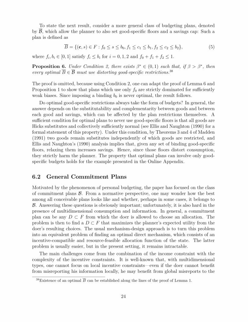
To state the next result, consider a more general class of budgeting plans, denotedby B, which allow the planner to also set good-specific floors and a savings cap: Such aplan is defined as

B = (c, s) ∈ F : f0 ≤ s ≤ b0, f1 ≤ c1 ≤ b1, f2 ≤ c2 ≤ b2, (5)

where fi, bi ∈ [0, 1] satisfy fi ≤ bi for i = 0, 1, 2 and f0 + f1 + f2 ≤ 1.

Proposition 6. Under Condition 2, there exists β∗ ∈ (0, 1) such that, if β > β∗, thenevery optimal B ∈ B must use distorting good-specific restrictions.38

The proof is omitted, because using Condition 2, one can adapt the proof of Lemma 6 andProposition 1 to show that plans which use only f0 are strictly dominated for sufficientlyweak biases. Since imposing a binding b0 is never optimal, the result follows.

Do optimal good-specific restrictions always take the form of budgets? In general, theanswer depends on the substitutability and complementarity between goods and betweeneach good and savings, which can be affected by the plan restrictions themselves. Asufficient condition for optimal plans to never use good-specific floors is that all goods areHicks substitutes and collectively sufficiently normal (see Ellis and Naughton (1990) for aformal statement of this property). Under this condition, by Theorems 3 and 4 of Madden(1991) two goods remain substitutes independently of which goods are restricted, andEllis and Naughton’s (1990) analysis implies that, given any set of binding good-specificfloors, relaxing them increases savings. Hence, since those floors distort consumption,they strictly harm the planner. The property that optimal plans can involve only good-specific budgets holds for the example presented in the Online Appendix.

6.2 General Commitment Plans

Motivated by the phenomenon of personal budgeting, the paper has focused on the classof commitment plans B. From a normative perspective, one may wonder how the bestamong all conceivable plans looks like and whether, perhaps in some cases, it belongs toB. Answering these questions is obviously important; unfortunately, it is also hard in thepresence of multidimensional consumption and information. In general, a commitmentplan can be any D ⊂ F from which the doer is allowed to choose an allocation. Theproblem is then to find a D ⊂ F that maximizes the planner’s expected utility from thedoer’s resulting choices. The usual mechanism-design approach is to turn this probleminto an equivalent problem of finding an optimal direct mechanism, which consists of anincentive-compatible and resource-feasible allocation function of the state. The latterproblem is usually easier, but in the present setting, it remains intractable.

The main challenges come from the combination of the income constraint with thecomplexity of the incentive constraints. It is well-known that, with multidimensionaltypes, one cannot focus on local incentive constraints—even if the doer cannot benefitfrom misreporting his information locally, he may benefit from global misreports to the

38Existence of an optimal B can be established along the lines of the proof of Lemma 1.

24

planner’s mechanism. One can try to apply the insights of the literature on multidi-mensional screening (cf Rochet and Stole (2003) for a survey) to the present problem,but substantive differences preclude this. First, in screening problems the mechanismdesigner can use transfers. Here, one can view the expected continuation utility fromsavings as a transfer and use Rochet and Choné’s (1998) dual approach to simplify the in-centive constraints and the planner’s objective. But the state-wise income constraint, thesecond key difference from screening problems, cannot be simplified. General techniquesexist for handling such constraints (for example, Luenberger (1969)). Unlike in the caseof unidimensional consumption (Amador et al. (2006)), however, here those techniquesdo not help to characterize the optimal mechanisms, which requires to jointly deter-mine the mechanism and the state-wise Lagrange multiplier for the income constraint.The solution need not follow the logic of the unidimensional case or of multidimensionalscreening, for which we know that solutions rarely exist in closed form and tend to havequite intricate structures even for simple settings.

Despite the loss of generality, the class of “interval plans” B (or B) remains of in-terest for several reasons. First, B is not fully general even in unidimensional settings,but in these settings, under weak conditions there exist optimal D ⊂ F which belongto B (Amador et al. (2006)).39 Hence, B represents a natural starting point to analyzemultidimensional settings. Second, in his seminal work on delegation problems—whichformally include the planner’s problem—Holmström (1977) noted that “one might wantto restrict D to [...] only certain simple forms of [policies], due to costs of using otherand more complicated forms or due to the fact that the delegation problem is too hard tosolve in general.” In his unidimensional settings, Holmström (1977) focused on intervalpolicies, because they “are simple to use with minimal amount of information and mon-itoring needed to enforce them” and “are widely used in practice.” In a similar spirit,discussing multidimensional delegation, Armstrong (1995) acknowledged that “in orderto gain tractable results it may be that ad hoc families of sets such as rectangles or circleswould need to be considered” (p. 20, emphasis in the original). Finally, for consumption-savings problems, Thaler and Shefrin (1981) argued that commitment “rules by naturemust be simple.” Simplicity is a property of budgeting plans, which also makes it eas-ier for people to stick to them40 and for third-party providers to market devices thatimplement them.

It may be worth considering other subclasses of commitment plans. The task, how-ever, will be to identify classes which not only are sensible, but also have enough structureto render the search of an optimal plan tractable. For instance, one may consider com-mitment plans defined by a binding boundary that smooths the kinks created by thebudgets and the savings floor in Figure 2(b). However, it is not obvious how to mathe-matically describe such a class and optimize over it. It is also not immediate that thisclass contains the overall optimal plan, because such a plan may involve interior bunchingregions as it often happens in multidimensional screening problems (Rochet and Choné

39Alonso and Matouschek (2008) and Amador and Bagwell (2013b) provide conditions for intervalpolicies to be globally optimal in other delegation settings with unidimensional decisions and information.

40Benhabib and Bisin (2005) provide a rationale for why people may prefer simple commitment rules,based on higher psychological costs of complying with complex rules.

25

(1998)). Finally, it may be hard for individuals to implement such complex plans, evenwith the help of third-party commitment devices.

6.3 Multiple Goods in Each Period

It is straightforward to generalize the model of Section 3 so that the individual consumes abundle of multiple goods in each period. Suppose that the function u(c; r) now representsthe consumption utility of both the planner and the doer in each period, where r continuesto represent the information affecting the intratemporal trade-offs. A state now includesthe realization of r in period 2 and so is given by (θ, r1, r2), where the superscripts referto the time period. In period 1, for each state the planner and the doer evaluate streams(c1, c2) using respectively the utility functions

θu(c1; r1) + u(c2; r2) and θu(c1; r1) + βu(c2; r2).The set of feasible allocations in period 1 and in period 2 are

F = (c1, s) ∈ R3+ : c1 + c2 + s ≤ 1

andF (s) = c2 ∈ R2

+ : c1 + c2 ≤ s, s ∈ [0, 1].

The family of budgeting plans for period 1, B1, is the same as B defined in Section 3.For period 2, a budgeting plan is defined as

B2 = c ∈ F (s) : c1 ≤ b1, c2 ≤ b2,where b1, b2 ∈ [0, 1].

As before, only the doer observes the state in each period. The timing changes asfollows. In period 1, first the planner commits to a plan B1, then the doer observes(θ, r1) and implements some allocation from B1. Given the chosen s, in period 2, firstthe planner commits to a plan B2, then the doer observes r2 and implements someallocation from B2. As Halac and Yared (2014) showed, information persistency overtime plays an important role in consumption-savings problems with imperfect self-control.However, to keep things simple, assume that here information is not persistent: r2 isindependently distributed from (θ, r1) according to the full-support probability measureG2 over the space Ω2 = [r1, r1] × [r2, r2]. Note that the timing involves the assumptionthat the individual has the power to commit within a period, but not across periods.This assumption is not innocuous, even without information persistency: By committingin period 1 to how B2 will depend on the chosen (c1, s), the planner may be able tomanage the doer’s bias in more effective ways. We will come back to this in Section 6.4.

Under these assumptions, it is easy to see that the planner will grant the doer fullflexibility in the last period. The reason is twofold: First, in period 2 both selves havethe same preferences; second, in period 1 the planner cannot commit to curtailing thedoer’s flexibility in period 2, so as to reward or punish his decisions in period 1. Formally,for every s inherited from period 1, the plan B2 = F (s) is optimal in period 2. Becauseof this, we can define the period-1 utility from savings v : [0, 1] → R by

v(s) =

ˆΩ2

[max

c∈F (s)u(c; r)

]dG2(r). (6)

26

This function satisfies some useful properties—summarized in Lemma 10 in the OnlineAppendix—which lead to the same analysis as in the simpler model used throughout thepaper.

6.4 Multi-Period Commitments

Consider now a model in which consumption involves multiple goods in each period (asin Section 6.3) and information is not persistent, but the planner can commit in period1 to the plans she will impose in period 2. In principle, by linking her period-2 plan tothe doer’s entire choice in period 1, (c1, s), the planner could use future punishments andrewards to better discipline him in the present; moreover, she could do so in ways thatare suboptimal ex post.

For such a model, one-period commitments entail no loss of generality if in eachperiod plans can be any set D of feasible allocations. This depends on two things (cfalso Amador et al. (2003)): (a) such plans can flexibly regulate how much the doer isallowed to save, possibly via money burning; (b) information is not persistent over time.To see this, imagine that for some (c1, s) the planner sets D(c1, s) ⊊ F (s) to punish thedoer in period 1. By (b), both selves assign the same expected payoff to D(c1, s), whichlies in the interval [u(0), v(s)]. Therefore, the planner can replace every (c1, s) in herperiod-1 plan with (c1, s′) and D(c1, s) with F (s′) for some s′ ≤ s—by (a)—so that sheand the doer get the same payoff from (c1, s) and (c1, s′) for every state; it is then optimalfor the doer to pick (c1, s′) whenever he was choosing the corresponding (c1, s), therebyproducing the same overall payoff for the planner. This is because the doer’s expectedpayoff from D(c1, s) does not depend on his period-1 information—by (b)—and hencecannot be used, in addition to c1 itself, to incentivize him to pick (c1, s) in some statesbut not in others. This point about one-period commitments is related to the findingin models with unidimensional consumption that the ex-ante and sequentially optimalplans coincide under non-persistent information (Amador et al. (2003, 2006)), but differunder persistent information (Halac and Yared (2014)). Lack of information persistency,however, is only part of the story here; property (a) also plays a key role, as it gives greatflexibility in managing continuation payoffs using one-period commitments. For instance,Breig (2015) studies another class of dynamic delegation problems with non-persistentinformation where ex-ante optimal mechanisms differ from the sequentially optimal ones.

If the planner can use only budgeting plans in B, the inability to commit for fu-ture periods may prevent her from achieving higher payoffs. This is because B violatesproperty (a). Note, however, that in settings where information is not persistent andaffects only the intertemporal trade-off, weak conditions ensure that the sequentially op-timal, unrestricted, plans D take the form of a minimum-savings rule in each period.41

Therefore, the main messages of the paper regarding good-specific budgets is unaffected.Furthermore, if in the present model the ex-ante optimal budgeting plans differed fromthe sequentially optimal ones, the substantive cause would again be the uncertainty about

41Amador et al. (2003) show this for the case of unidimensional consumption and the result can beextended to the case of multidimensional consumption using the ideas in Section 5.

27

intratemporal trade-offs.

6.5 Multiple Future Periods

Not surprisingly, extending the model beyond two periods adds intricacies to the analysis,which however do not distinguish this paper from the literature. The following are themost substantive.

When the future has multiple periods, the expected continuation utility from sav-ing, v, depends on the future commitment plans as well as the intensity of presentbias, β. In each period (except possibly the last one), the planner commits to plansthat curtail the doer’s discretion and hence influence the value of entering that periodwith savings s. Such a value also depends on β, as β affects the chosen plan as well as thedoer’s behavior. The dependence on β of the marginal value of having one extra dollarnext period ultimately affects the planner’s desire to curb undersaving in this period: Astronger bias induces the doer to undersave more in the present, thereby strengtheningthat desire; at the same time, it may also reduce the marginal value of savings—due toworse future allocations—thereby weakening that desire.

Nonetheless, optimal budgeting plans should continue to involve good-specific bud-gets for sufficiently weak biases, but only a savings floor f for sufficiently strong biases.Consider any intermediate period. Intuitively, for β close to 1 the planner should againwant to set a very slack f when this is the only tool available. Such an f would againgrant the doer full discretion in states that call for high consumption of only some good.In this case, setting a good-specific budget strictly improves on using only f for the samereasons highlighted above. On the other hand, for β close to zero budgets cannot increasesavings but distort consumption; hence, plans which use budgets are strictly dominatedby those which use only f .

A second issue, discussed also by Amador et al. (2003), is that an infinite-horizonmodel may have multiple equilibria of the game between the individual’s selves. Thisissue is well-known and orthogonal to the message of the present paper. The pointremains valid that distorting restrictions on consumption (on top of savings restrictions)can be useful tools to discipline the doer. Such distortions should therefore appear as anovel feature in at least some equilibria of the multi-self game.

7 Other ApplicationsThe insights offered by the planner-doer problem can be applied to other settings. Forthese applications the theory can assume a more normative flavor, while keeping in mindthe limitations of the simple class of budgeting policies considered in this paper.

Public Finance. Consider first a public-finance application along the lines of Halacand Yared (2014). In each period, a government chooses how much to spend on a list ofpublic goods and services, c, and how much to save or borrow, s, subject to the constraintgiven by the tax revenues. The government may exhibit present bias as a consequence of

28

aggregating the preferences of heterogeneous citizens (Jackson and Yariv (2015)) or dueto uncertainty in the political turnover (Aguiar and Amador (2011)). For this setting, thetheory developed in Section 4 can explain why governments often set limits on borrowing(for example, via budget-deficit ceilings), but also specific limits on some good or serviceexpenses (for example, via fiscal budgets). The theory shows when and why combiningdeficit ceilings with fiscal budgets can dominate policies that rely only on the ceilings. Atthe same time, it shows that fiscal budgets are no free lunch: They can cause inefficienciesin public spending, which however play a key role in curtailing overborrowing. Of course,fiscal budgets can just be part of accounting techniques. This theory, however, adds adifferent perspective on the functions that such budgets can have.

More generally, the problem studied in this paper can be viewed as an instance ofa multidimensional delegation problem where a principal delegates to a better-informedagent the allocation of a finite amount of resources (money or time) to multiple categoriesof expenditures. Also, it is not essential that the consequences of the agent’s allocationhappen at different dates: They can all happen within the same period, and the conflictof interest between the principal and the agent need not stem from time preferences. Thefollowing situations illustrate this.

Corporate Governance. The owner of a company appoints a manager, who eachperiod decides how to allocate some total resources between spending on sales activities, y,and investment in R&D, x0. The company sells two products and the manager alsochooses which share of y goes to promoting which product (x1 and x2). Let F = x ∈R3

+ : x0+x1+x2 ≤ 1 be the set of all feasible allocations. The manager privately observesinformation on the returns to marketing each product and from investing in R&D. Letthis information be represented by state ω = (ω0, ω1, ω2), where 0 < ωi ≤ ωi ≤ ωi < +∞for all i. Finally, as a result of compensation schemes or career goals, the manager maycare more or less about cash flows—and hence about sales vs. R&D—than does theowner.

We can express the owner’s problem of delegating to the manager the allocation ofresources as follows: Choose D ⊂ F to maximize

U(D) =

ˆΩ

[ω0u0(x0(ω)) + ω1u

1(x1(ω)) + ω2u2(x2(ω))]dG(ω) (7)

subject to

x(ω) ∈ argmaxx∈D

[βω0u

0(x0) + ω1u1(x1) + ω2u

2(x2)], ω ∈ Ω. (8)

The parameter β > 0 represents the conflict of interest between parties. Note that, asin the main model the planner and the doer disagreed on the importance of consumingvs. savings within each period, here the owner and the manager disagree regarding theimportance of sales vs. R&D activities; but given R&D investment x0, they agree on howto divide the remaining resources to promote each product.

To illustrate, suppose that the manager undervalues R&D (that is, β < 1) and thatdelegation policies are restricted to B. This paper suggests that to best incentivize themanager, the owner may have to impose limits on how much can be spent each period onpromoting specific products, possibly in addition to requiring a minimum investment in

29

R&D. Due to these limits, the manager may end up promoting some product too littleand the other too much. This, however, is a risk the owner should take, as it is morethan compensated in expectation by better allocations to R&D. A detailed budget planwith rules applying to specific products is more likely to benefit the owner when sheagrees sufficiently with the manager on how important R&D is. This may be true, forinstance, if the manager himself has significant stakes in the company. Otherwise, theowners should simply demand only a minimum investment in R&D.

Fiscal-constitution Design. Society delegates a government to divide the economyresources between private consumption, x0, and public spending, y. The government in-corporates the preference of a representative agent in society, but is biased in favor ofpublic spending (β < 1).42 This bias may depend on incentives created by political insti-tutions, for instance. The government spends y to fund two services (x1 and x2). Despiteits bias, at a first approximation it may not favor any service more than others, and thusagrees with society on how to allocate any level of public spending between services.43

The government acts on non-contractible information, ω, which affects the social valueof each service (for example, the gravity of national-security threats or natural disas-ters), as well as the overall trade-off between private consumption and public spending(for example, the state of the business cycle). In this case, behind a veil of ignorancesociety may want to design a fiscal constitution—a delegation policy D—that restrictswhich allocations the government can choose. This problem can again be expressed by(7) and (8).

Suppose society can choose only policies in B. The analysis shows that if the gov-ernment’s bias is weak, then an optimal fiscal constitution must involve service-specificspending caps. Such caps work because they cause inefficiencies in the composition ofpublic spending, thereby weakening the government’s desire to spend. But from society’sviewpoint, these inefficiencies are more than compensated by the resulting higher level ofprivate consumption. On the other hand, if the government is strongly biased, the consti-tution should involve only an aggregate spending cap (or a private-consumption floor).This is because any binding specific cap distorts public spending without sufficientlyimproving private consumption.

Workforce Management. An employer (she) hires a worker (he) under a contractspecifying a fixed wage and number of hours per workday. The worker performs two tasksand chooses how to allocate time between them (x1 and x2). He can also take breaks,represented by x0. The worker privately observes information on which task demandsmore attention. Given this, the employer delegates to him his time allocation. However,the worker weighs his break time more than does the employer (β > 1). Thus, she maywant to set up some rules to restrict his choices, modeled as a subset D of all feasibletime allocations. Expressions (7) and (8) again capture the employer’s problem.

Suppose that she can use only budgeting policies. An analysis similar to that above42This hypothesis is supported by theoretical as well as empirical work in the political-economy liter-

ature (Niskanen (1975), Romer and Rosenthal (1979), Peltzman (1992), Funk and Gathmann (2011)).43This property is arguably strong, but is consistent with some empirical evidence. For example,

Peltzman (1992) finds that U. S. voters penalize federal spending growth, but its composition seemsirrelevant, which suggests that “every extra dollar is equally bad.”

30

leads to results in which caps and floors swap roles. A floor on task i induces the workerto allocate less time to x0, but also less time to the other task. Nonetheless, if theworker’s tendency to indulge in breaks is weak, an optimal policy must involve bindingtask-specific floors. By contrast, if the worker’s bias is strong, the employer shouldimpose only a cap b0 on x0. In practice, it may be impossible to monitor the worker’sbreaks; however, b0 can be implemented via an overall minimum time that the workerhas to allocate to his tasks, which may be easier to monitor. The theory shows that thepossibility of monitoring each task individually may allow the employer to design strictlysuperior policies by adding individual floors.

8 Concluding RemarksThis paper provides a theoretical analysis of the relationship between self-control prob-lems and personal budgeting using a simple consumption-savings model which intro-duces no “behavioral” or ad-hoc feature besides a standard form of present bias. Unlikeminimum-savings rules, good-specific spending caps help to curtail overspending becausethey cause inefficiencies in consumption which lower the return from undersaving, therebycounteracting present bias. Consequently, good-specific budgets are no free lunch andare used only by consumers who are weakly biased and ex-ante uncertain about theirintratemporal trade-offs between goods. Those who are strongly biased or do not facesuch uncertainty prefer to rely exclusively on a minimum-savings rule.

This theory offers solid insights into the subtle forces underlying a widely observedphenomenon, which has far-reaching consequences for consumer behavior and welfare byaffecting demand in different ways from satiation and income effects and by significantlycontributing to households’ wealth accumulation. The theory matches existing empir-ical findings, such as that many people set budgets for goods normally not viewed astemptations and that only people who exhibit weak present bias seem to use budgets.The theory also suggests new directions for enriching this limited evidence on personalbudgeting by demonstrating its key dependence on uncertain intratemporal trade-offs,and for designing commitment devices whose functions are targeted to the right type ofpresent-biased individuals.

From a normative perspective, the paper does not show that optimal commitmentplans within the universe of all possible plans turn out to take the form of budgeting.This result seems very unlikely to hold and was not the goal of the paper to beginwith. Technical difficulties aside, it seems more plausible that fully optimal plans arequite complicated and sensitive to details of the environment. This complexity mayundermine an individual’s ability to stick to a plan and hence should be traded offwith its capacity of solving self-control problems. Analyzing this trade-off is beyond thescope of this paper. In practice, individuals may have settled for personal budgetingas a viable compromise based on robustness, learning, or some heuristics. Of course,this explanation is less satisfactory for the application of the theory to other, formallyequivalent, delegation problems within organizations—which may, however, still valuesimplicity. Future research may benefit from the insights of this paper to build a general

31

normative theory of how to delegate multidimensional allocations of finite resources.

9 Appendix: Proofs

9.1 Proof of Proposition 1

The proof relies on the following four lemmas. Hereafter, for k = p, d, let sk = minω sk(ω) andsk(ω) = maxω sk(ω).

For any floor f ∈ [sd, sp],44 denote by Bf the corresponding policy in B.

Lemma 3. Define Ω(f) = ω ∈ Ω : sd(ω) ≤ f and

cf (ω) = argmaxc∈Rn

+:∑n

i=1 ci≤1−fu(c; r), ω ∈ Ω.

The payoff U(Bf ) is differentiable in f over the domain [sd, sp] with

d

dfU(Bf ) =

ˆΩ(f)

[v′(f)− θ

∂

∂ciu(cf (ω); r)

]dG,

for any i = 1, . . . , n.

Proof. For simplicity, let Ψ(f) = U(Bf ). Also, we will consider only f ∈ [sd, sp] withoutrepeating this every time. Given f and any ω, define

u(f ;ω) ≡ u(cf (ω); r) = maxc∈Rn

+:∑n

i=1 ci≤1−fu(c; r). (9)

and U(f ;ω) = θu(f ;ω)+v(f). Since u(·; r) is strictly concave in c, so is u(·; r) in f by standardarguments. This implies that U(·;ω) is also strictly concave in f .

Now consider the derivative of U(f ;ω) with respect to f . Whenever it is defined, we have

U ′(f ;ω) = θu′(f ;ω) + v′(f).

The first-order conditions of the Lagrangian defining u(f ; r) say that ∂∂ci

u(cf (ω); r) = λ(ω; f)for i = 1, . . . , n, where λ(ω; f) is the Lagrange multiplier for the constraint

∑ni=1 ci ≤ 1 − f .

Since cf (ω) is continuous in f for every ω, so is λ(ω; f) given our assumptions on u. By Theorem1, p. 222, of Luenberger (1969), for every f ′, f ′′ ∈ (0, 1) we have

λ(ω; f ′)(f ′′ − f ′) ≤ u(f ′; r)− u(f ′′; r) ≤ λ(ω; f ′′)(f ′′ − f ′).

Continuity of λ(ω; ·) then implies that ∂∂f u(f ; r) exists for every f ∈ (0, 1) and satisfies

∂

∂fu(f ; r) = −λ(ω; f) = − ∂

∂ciu(cf (ω); r).

Therefore,U ′(f ;ω) = v′(f)− θ

∂

∂ciu(cf (ω); r), ω ∈ Ω. (10)

44Any other floor is dominated by one in this range.

32

For any f , denote by (cf , sf ) the doer’s behavior as a function of ω under policy Bf . Notethat (cf (ω), sf (ω)) is continuous in both f and ω by the Maximum Theorem. Since, given anychoice of s, the planner and the doer would choose the same c in every ω, by definition we have

Ψ(f) =

ˆΩU(sf (ω);ω)dG.

Consider any f > f and recall that Ω(f) = ω : sd(ω) ≤ f. Then,

Ψ(f)−Ψ(f) =

ˆΩ

[U(sf (ω);ω)− U(sf (ω);ω)

]dG

=

ˆΩ(f)

[U(f ;ω)− U(sf (ω);ω)

]dG

=

ˆΩ(f)∩(Ω(f))

c

[U(f ;ω)− U(sf (ω);ω)

]dG

+

ˆΩ(f)

[U(f ;ω)− U(f ;ω)

]dG.

where the second equality follows because sf (ω) = sf (ω) for ω /∈ Ω(f) and sf (ω) = f forω ∈ Ω(f). Dividing both sides by f − f , we get

limf↓f

Ψ(f)−Ψ(f)

f − f= lim

f↓f

ˆΩ(f)

U(f ;ω)− U(f ;ω)

f − fdG (11)

+ limf↓f

ˆΩ(f)∩(Ω(f))

c

U(f ;ω)− U(sf (ω);ω)

f − fdG.

Consider the first limit. For all ω, we have

limf↓f

U(f ;ω)− U(f ;ω)

f − f= U ′(f ;ω).

Since U(·;ω) is concave,∣∣∣∣∣ U(f ;ω)− U(f ;ω)

f − f

∣∣∣∣∣ ≤ max∣∣∣U ′(f ;ω)

∣∣∣ , ∣∣∣U ′(f ;ω)∣∣∣ .

Since U ′(f ;ω) is continuous in ω and f as illustrated by (10),

max(f,ω)∈[sd,sp]×Ω

∣∣∣U ′(f ;ω)∣∣∣ = M < +∞.

Therefore, by Lebesgue’s Bounded Convergence Theorem, we have

limf↓f

ˆΩ(f)

U(f ;ω)− U(f ;ω)

f − fdG =

ˆΩ(f)

U ′(f ;ω)dG.

Consider now the second limit in (11). Again, by concavity of U(·;ω) and since sf (ω) ∈[sd, sp] for f ∈ [sd, sp], we have that∣∣∣∣∣ U(f ;ω)− U(sf (ω);ω)

f − sf (ω)

∣∣∣∣∣ ≤ M.

33

Therefore,∣∣∣∣∣ˆΩ(f)∩(Ω(f))

c

U(f ;ω)− U(sf (ω);ω)

f − fdG

∣∣∣∣∣ ≤ˆΩ(f)∩(Ω(f))

c

∣∣∣∣∣ U(f ;ω)− U(sf (ω);ω)

f − f

∣∣∣∣∣ dG≤ˆΩ(f)∩(Ω(f))

c

∣∣∣∣∣ U(f ;ω)− U(sf (ω);ω)

f − sf (ω)

∣∣∣∣∣ dG≤ M

ˆΩ(f)∩(Ω(f))

cdG.

Now, observe that Ω(f) ∩(Ω(f)

)c= ω : f < sf (ω) ≤ f which converges to an empty set as

f ↓ f . It follows that the second limit in (11) converges to zero as f ↓ f . We conclude that forevery f ∈ [sd, sp), we have

Ψ′(f+) =

ˆΩ(f)

U ′(f ;ω)dG.

Now consider any f < f . Then,

Ψ(f)−Ψ(f) =

ˆΩ

[U(sf (ω);ω)− U(sf (ω);ω)

]dG

=

ˆΩ(f)

[U(sf (ω);ω)− U(f ;ω)

]dG

=

ˆΩ(f)

[U(f ;ω)− U(f ;ω)

]dG+

ˆΩ(f)

[U(sf (ω);ω)− U(f ;ω)

]dG

=

ˆΩ(f)

[U(f ;ω)− U(f ;ω)

]dG+

ˆΩ(f)∩(Ω(f))

c

[U(sf (ω);ω)− U(f ;ω)

]dG,

where the second equality follows because sf (ω) = sf (ω) for ω /∈ Ω(f) and sf (ω) = f forω ∈ Ω(f), and the last equality follows because sf (ω) = f for ω ∈ Ω(f). By the same argumentas before,

limf↑f

ˆΩ(f)

U(f ;ω)− U(f ;ω)

f − fdG =

ˆΩ(f)

U ′(f ;ω)dG,

limf↑f

ˆΩ(f)∩(Ω(f))

c

U(sf (ω);ω)− U(f ;ω)

f − fdG = 0.

We conclude that for everyf ∈ (sd, sp], we have

Ψ′(f−) =

ˆΩ(f)

U ′(f ;ω)dG.

Hence, Ψ(f) is differentiable over the restricted domain [sd, sp].

We now consider how the planner would use only the floor f .

Lemma 4. When the planner can set only a floor on s, every optimal f lies strictly betweensp and sp.

34

Proof. We will show that Ψ′(f) > 0 for all f ∈ (sd, sp] and Ψ′(f−) < 0 for f = sp. Recall that(cf , sf ) is continuous in f for every ω and therefore Ψ(f) is continuous in f . These observationswill imply that every optimal f∗ is in (sp, sp).

For any f ∈ (sd, sp], define

Ω+(f) = ω : sp(ω) > f and Ω−(f) = ω : sp(ω) ≤ f.

For ω ∈ Ω+(f), consider the the following fictitious problem in which the planner is forced tosave less than f :

max(c,s)∈Rn+1

+

θu(c; r) + v(s)

subject to s+∑

i ci ≤ 1 and s ≤ f . The associated Lagrangian is

θu(c; r) + v(s) + µ(ω)

[1− s−

n∑i=1

ci

]+ ϕ+(ω)[f − s].

Hence, the first-order conditions are45

v′(s) = µ(ω) + ϕ+(ω) and θ∂

∂ciu(c; r) = µ(ω) for all i.

Clearly, the constraint s ≤ f must bind for ω ∈ Ω+(f), which implies that s = f and ϕ+(ω) > 0.Also, conditional on choosing s = f , the planner and the doer would choose the same c in stateω, which therefore equals cf (ω). Using (10), it follows that, for every i,

ϕ+(ω) = v′(f)− θ∂

∂ciu(cf (ω);ω) = U ′(f ;ω) (12)

when ω ∈ Ω+(f).For ω ∈ Ω−(f), consider the following fictitious problem in which the planner is forced to

save more than f :max

(c,s)∈Rn+1+

θu(c; r) + v(s)

subject to s+∑

i ci ≤ 1 and s ≥ f . Again, the associated Lagrangian is

θu(c; r) + v(s) + µ(ω)

[1− s−

n∑i=1

ci

]+ ϕ−(ω)[s− f ].

Hence, the first-order conditions are

v′(s) = µ(ω)− ϕ−(ω) and θ∂

∂ciu(c; r) = µ(ω) for all i,

Clearly, the constraint s ≥ f must bind for ω ∈ Ω−(f) except when sp(ω) = f , which impliesthat s = f and ϕ−(ω) ≥ 0. Also, conditional on choosing s = f , the planner and the doerwould choose the same c in state ω, which therefore equals cf (ω). Using (10), it follows that,for every i,

ϕ−(ω) = θ∂

∂ciu(cf (ω); r)− v′(f) = −U ′(f ;ω)

45Here, as well as in the other proofs, the complementary slackness conditions are omitted for sim-plicity.

35

when ω ∈ Ω−(f).Consider any f ∈ (sd, sp]. Recall that Ω(f) = ω : sd(ω) ≤ f. Using Lemma 3, we have

Ψ′(f) =

ˆΩ(f)

U ′(f ;ω)dG

=

ˆΩ(f)∩Ω+(f)

U ′(f ;ω)dG+

ˆΩ(f)∩Ω−(f)

U ′(f ;ω)dG

=

ˆΩ(f)∩Ω+(f)

ϕ+(ω)dG,

where the last equality follows because either Ω−(f) = ∅ or ϕ−(ω) = 0 for ω ∈ Ω−(f). Thefunction ϕ+(ω) is strictly positive over Ω(f)∩Ω+(f). We need to show that this set has strictlypositive measure, which implies Ψ′(f) > 0. This is immediate if f ∈ (sd, sp), because in thiscase Ω+(f) = Ω. Consider f = sp. Clearly, Ω(sp) ∩ Ω+(sp) contains the open set

Ω(sp) ∩ Ω+(sp) = ω : sd(ω) < sp < sp(ω).

If we can show that this set is non-empty, we are done because G assigns strictly positiveprobability to it. Both Ω

(sp) and Ω+(sp) are nonempty. Suppose that there is no ω ∈ Ω+(sp)

such that we also have ω ∈ Ω(sp). Then, it means that for every ω ∈ Ω+(sp), we have

sd(ω) ≥ sp and that Ω(sp) ⊂ Ω−(sp) = ω : sp(ω) = sp. Now, consider ω ∈ Ω

(sp) and any

sequence ωn in Ω+(sp) converging to ω. We have that

limωn→ω

inf sd(ωn) ≥ sp > sd(ω).

But this violates the continuity of sd and hence leads to a contradiction.Now consider f = sp. Using again Lemma 3, we have

Ψ′(sp−) =

ˆΩ(sp)

U ′(sp;ω)dG =

ˆΩU ′(sp;ω)dG = −

ˆΩϕ−(ω)dG,

where ϕ−(ω) > 0 for all ω such that sp(ω) < sp. Therefore, Ψ′(sp−) < 0.46

We now consider how an optimal f varies with β. Recall that u∗(y; r) is the indirect utilityof spending y ∈ [0, 1] on consumption.

Lemma 5. The set of optimal floors, denoted by E(β), is decreasing in β in the strongset order.47 In particular, the largest optimal floor converges monotonically to sp as β ↑ 1.Moreover, there exists β > 0 such that E(β) = f for all β ≤ β, where f satisfies f < sp and

U(Bf ) = maxf∈[sp,sp]

ˆΩ[θu∗(1− f ; r) + v(f)]dG.

46It is easy to see that the optimal f satisfies f ≤ sp. Suppose f ∈ (sp, 1). Then, for all ω, the doerchooses s(ω) = f and c(ω) = cf (ω). Take any f ′ ∈ (sp, f). Then, for every ω, f ′ = ζ(ω)f + (1 −ζ(ω))sp(ω) for some ζ(ω) ∈ (0, 1). Therefore, for every ω, U(f ′;ω) > U(f ;ω) because U(sp(ω);ω) >U(f ;ω) and U(·;ω) is strictly concave. It follows that the planner’s payoff is strictly larger under f ′

than under f .47Given two sets E and E′ in R, E ≥ E′ in the strong set order if, for every f ∈ E and

f ′ ∈ E′, minf, f ′ ∈ E′ and maxf, f ′ ∈ E (Milgrom and Shannon (1994)).

36

Proof. Fix f ∈ [sd, sp]. The set Ω(f) in Lemma 3 depends on β via (cd, sd). By standardarguments, if β < β′ < 1, then sd(ω;β) < sd(ω;β′) for every ω and hence Ω(f ;β′) ⊂ Ω(f ;β).On the other hand, for every β < 1, we have Ω−(f) ⊂ Ω(f ;β) because sd(ω;β) < sp(ω) forevery ω. So, if β < β′ < 1, we have

Ψ′(f ;β)−Ψ′(f ;β′) =

ˆ(Ω(f ;β)\Ω(f ;β′))∩Ω+(f)

ϕ+(ω)dG ≥ 0,

where the inequality follows from (12). Standard monotone-comparative-static results thenimply that E(b) is increasing in the strong set order.

Define f(β) = maxf : f ∈ E(β). Since f(β) ≥ sp for all β and f(·) is decreasing,limβ↑1 f(β) exists; denote it by f(1−) ≥ sp. Clearly, f(1) = sp. Now suppose that f(1−) >f(1). By a similar argument, for any f > sp, limβ↑1Ψ

′(f ;β) exists and satisfies

limβ↑1

Ψ′(f ;β) = −ˆΩ−(f)

ϕ(ω)dG < 0.

This implies that for β close enough to 1, f(β) ≥ f(1−) cannot be optimal, a contradictionwhich implies that f(1−) = f(1).

It is easy to see that, for all ω ∈ Ω, sd(ω;β) → 0 as β ↓ 0. Therefore, sd(β) = maxΩ sd(s;β)also decreases monotonically to 0 as β ↓ 0. Let β = maxβ ∈ [0, 1] : sd(β) ≤ sp which isstrictly positive because sp > 0. Then, Ω(f) = Ω for all β ≤ β and f ∈ [sp, sp], which impliesthat

Ψ(f ;β) =

ˆΩ[θu(cf (ω); r) + v(f)]dG. (13)

From the proof of Lemma 3, we have that u(cf (ω); r) = u(f ;ω) is strictly concave in f for allω ∈ Ω. This implies that the maximizer of (13) is unique. From the proof of Lemma 4, weknow that the derivative of (13) is negative at sp and hence f < sp.

We now show that the planner benefits from imposing only one budget on any good.

Lemma 6. Fix i and consider plans Bbi with bj = 1 for all j = i and f = 0. There exists bi <maxω cdi (ω) ≡ cdi such that the planner strictly benefits from it, that is, U(Bbi) > U(F ).

Proof. Fix i = 1 and consider any b1 ∈ (0, cd1]. Let (cb1 , sb1) describe the doer’s choices undercap b1. Then, let

Φ(b1) =

ˆΩ[θu(cb1(ω); r) + v(sb1(ω))]dG.

Let Ω(b1) = ω : cd1(ω) > b1. Note that for any b1 < cd1, since cd1 is continuous, Ω(c1) isnon-empty and open, and hence has strictly positive probability under G. We have

Φ(b1)− Φ(cd1) =

ˆΩ(b1)

[θu(cb1(ω); r) + v(sb1(ω))]− [θu(cd(ω); r) + v(sd(ω))]dG

= (1− β)

ˆΩ(b1)

[v(sb1(ω))− v(sd(ω))

]dG

+

ˆΩ(b1)

[V (cb11 (ω);ω)− V (cd1(ω);ω)

]dG,

37

whereV (b1;ω) = max

(c,s)∈Rn+1+ :

∑nj=1 cj≤1,c1≤b1

θu(c; r) + βv(s).

Clearly, V (cd1(ω);ω) ≥ V (b1;ω) for every ω. From the first-order conditions of the Lagrangiandefining V (b1;ω), we have λ1(ω; b1) = θu1c(c

b11 (ω); r1) − βv′(sb1(ω)), where λ1(ω; b1) is the

Lagrange multiplier on the constraint c1 ≤ b1. Since (cb1(ω), sb1(ω)) is continuous in b1 as wellas ω, so is λ1(ω; b1). Relying again on Theorem 1, p. 222, of Luenberger (1969), we concludethat V ′(b1;ω) exists for every b1 and equals λ1(ω; b1). It follows that V ′(cd1(ω);ω) = 0 for everyω by the definition of (cd, sd). Therefore, by the Mean Value Theorem (MVT),

V (cb11 (ω);ω)− V (cd1(ω);ω) = V ′(χ(ω);ω)(cb11 (ω)− cd1(ω)),

v(sb1(ω))− v(sd(ω)) = v′(ξ(ω))(sb1(ω)− sd(ω)),

where χ(ω) ∈ [cb11 (ω), cd1(ω)] and ξ(ω) ∈ [sd(ω), sb1(ω)].Let bε1 = cd1 − ε for some small ε > 0. Fix any ω ∈ Ω(bε1) and, for now, suppress the

dependence on ω for simplicity. Recall that sbε1 +∑

i cbε1i = sd +

∑i c

di = 1. Since sb

ε1 > sd for

any ε > 0 (cf Lemma 9), we can write

− cbε11 − cd1sb

ε1 − sd

= 1 +∑j =1

cbε1j − cdj

sbε1 − sd

. (14)

Now, for any bε1, the following first order condition must hold for every j = 1:

βv′(s)− θujc(cj ; rj) = 0.

Therefore, using again the MVT, for all j = 1 we have

cbε1j − cdj =

β[v′(sbε1)− v′(sd)]

θujcc(ζj ; rj)(15)

for some ζ ∈ [cdj , cbε1j ]. Now, since v′′ is continuous, we have that v′(y) − v′(y) ≥ v′′[y − y] for

every y > y ≥ sd, where v′′ = minξ∈[sd,1] v′′(ξ) < 0. Therefore, using (14) and (15), we havethat

− cbε11 − cd1sb

ε1 − sd

= 1 +1

sbε1 − sd

∑j =1

β

θujcc(ζj ; rj)[v′(sb

ε1)− v′(sd)]

≤ 1 +1

sbε1 − sd

∑j =1

βv′′

θujcc(ζj ; rj)[sb

ε1 − sd]

≤ 1 +βv′′

θ

∑j =1

1

ujcc,

where the first inequality uses the fact that ujcc < 0 and ujcc = maxξ∈[sd,1],rj∈[rj ,rj ] ujcc(ξ; rj) < 0

(which is well defined by continuity of ujcc). Thus, letting K =[1 + βv′′

θ

∑j =1

1

ujcc

]−1> 0, it

follows that for every ω ∈ Ω(bε1),

sbε1(ω)− sd(ω) ≥ K

[cd1(ω)− c

bε11 (ω)

].

38

Using these observations, we have that Φ(bε1)− Φ(cd1) is bounded below byˆΩ(bε1)

[K(1− β)v′(ξ(ω))− V ′(χ(ω);ω)

](cd1(ω)− bε1)dG. (16)

Since v′ is continuous and strictly positive everywhere and ξ(ω) ∈ [sd, 1] with sd > 0 for allω ∈ Ω(bε1), there exists a finite κ > 0 such that v′(ξ(ω)) ≥ κ for all ω ∈ Ω(bε1).

Next let Ω(bε1) = ω : cd1(ω) ≥ bε1 which is a closed and bounded set by continuity of cd1and hence is compact. As a function of bε1, the correspondence Ω(·) is continuous by continuityof cd1. Note that, if cd1(ω) = bε1, then V ′(χ(ω);ω) = V ′(cd1(ω);ω) = 0. We have

supω∈Ω(bε1)

V ′(χ(ω);ω) = supω∈Ω(bε1)

V ′(χ(ω);ω) ≤ maxbε1≤ζ≤cd1,ω∈Ω(bε1)

V ′(ζ;ω) ≡ κ(bε1).

Clearly, κ(bε1) ≥ 0 for every ε > 0, ε′ > ε > 0 implies that κ(bε1) ≤ κ(bε′1 ), and limε→0 κ(b

ε1) = 0

because κ(·) is also continuous. Therefore, there exists ε∗ > 0 such that

κ(bε∗1 ) < κ(1− β)K.

It follows that for ε∗, expression (16) is strictly positive, and hence Φ(bε∗1 ) > Φ(cd1). This also

holds for all ε ∈ (0, ε∗).

We can now complete the proof of Proposition 1. By Lemma 5, f(β) decreases monoton-ically to sp when β ↑ 1. Also, for every i = 1, . . . , n, we have that sd(θ, ri, r−i;β) increasesmonotonically to sp(θ, ri, r−i) as β ↑ 1. By Remark 1, sp(θ, ri, r−i) > sp. Given this, define

β∗ = infβ ∈ (0, 1) : f(β) < maxi

sd(θ, ri, r−i;β).

Clearly, β∗ < 1 and, for every β > β∗, we have sd(θ, ri, r−i;β) > f(β) for at least somei = 1, . . . , n. Hereafter, fix β > β∗ and any i that satisfies this last condition.

For ε ≥ 0, consider bεi = cdi − ε as in Lemma 6 where cdi = cdi (θ, ri, r−i) by Remark 1. LetΦ(bεi , f(β)) be the planner’s expected payoff from adding bεi to the existing optimal floor f(β).We will show that there exists ε > 0 such that Φ(bεi , f(β)) > Φ(b0i , f(β)) where Φ(b0i , f(β)) =U(Bf(β)). To do so, for any ε ≥ 0, let (cε, sε) be the doer’s allocation function under (bεi , f(β))and Ω(bεi ) = ω ∈ Ω : c0i (ω) > bεi. Then,

Φ(bεi , f(β))− Φ(b0i , f(β)) =

ˆΩ(bεi )

[θu(cε(ω); r) + v(sε(ω))]− [θu(c0(ω); r) + v(s0(ω))]dG.

Note that, if there exists ε > 0 such that for all 0 < ε < ε we have (cε(ω), sε(ω)) = (cd(ω), sd(ω))for all ω ∈ Ω(bεi ), then for such ε’s the previous difference equals Φ(bεi ) − Φ(cdi ) in the proofof Lemma 6. The conclusion of that proof then implies that there exists ε∗∗ ∈ (0, ε) such thatΦ(bε

∗∗i , f(β)) > Φ(b0i , f(β)).Thus we only need to prove the existence of ε. Let Ω(f(β)) = ω ∈ Ω : sd(ω) ≤ f(β),

which is compact by continuity of sd. Define ci = maxΩ(f(β)) c0i (ω) which is well defined by

continuity of c0. Since sd(θ, ri, r−i) > f(β), it follows that (θ, ri, r−i) /∈ Ω(f(β)) and hence

39

c0i (θ, ri, r−i) = cdi (θ, ri, r−i) where cdi (θ, ri, r−i) = cdi by Remark 1. We must also have ci < cdi :for all ω ∈ Ω(f(β)), optimality requires

θuic(ci(ω); ri) = βv′(f(β)) + λ0(ω) > βv′(sd(θ, ri, r−i)) = θuic(cdi ; ri),

where λ0(ω) ≥ 0 is the Lagrange multiplier for constraint s ≥ f(β). If ω ∈ Ω is such thatc0i (ω) > ci, then ω /∈ Ω(f(β))—otherwise it would contradict the definition of ci—and thereforec0(ω) = cd(ω). Now define ε = cdi − ci > 0. By construction for every ε ∈ (0, ε), c0i (ω) > bεiimplies that c0(ω) = cd(ω), as desired.

9.2 Proof of Proposition 2 and Corollary 1

Lemma 7. For every β ∈ (0, 1), if B ∈ B is optimal, then maxf, 1−∑n

i=1 bi ≥ minω∈Ω sp(ω).

Proof. Define

σ = maxf, 1−n∑

i=1

bi

Given this, we have that s(ω) +∑n

i=1 ci(ω) = 1, and hence s(ω) ≥ σ for all ω ∈ Ω. Withoutloss of generality, we can let σ = minΩ s(ω): If minΩ s(ω) > σ, we could simply raise f to thelevel minΩ s(ω) and nothing would change.Now fix β ∈ (0, 1). Suppose B′ is optimal, but σ′ < sp. Consider B′′ ∈ B identical to B′, exceptthat f ′′ = sp. Since B′ is convex and compact, the ensuing allocation (c′, s′) is a continuousfunction of ω. Hence, the set Ω(sp) = ω ∈ Ω : s′(ω) < sp contains an open subset and hencehas strictly positive probability under G.Consider any ω ∈ Ω(sp). Suppose the planner faces the following problem:

max(c,s)∈Rn+1

+

θu(c; r) + v(s)

subject to ci ≤ b′i, and s ≤ f . For any f < sp, the latter constraint must bind because, by thesame logic of Lemma 9, the planner would want to save at least sp(ω) ≥ sp if facing only theconstraints ci ≤ b′i for i = 1, . . . , n. Therefore, the planner’s payoff from this fictitious problemis strictly increasing in f for f ≤ sp. When the doer faces B′′, the constraint s ≥ sp must bind.Hence, his allocation (c′′(ω), sp) solves maxu(c; r) subject to c ∈ Rn

+, ci ≤ b′i, and∑n

i=1 ci ≤1− sp. This allocation coincides with the planner’s allocation under the fictitious problem withf = sp. Hence, in ω, (c′′(ω), sp) is strictly better for the planner than (c′′(ω), s′(ω)).We conclude that, for all ω ∈ Ω(sp), the planner’s payoff is strictly larger under B′′ than underB′. Since for ω /∈ Ω(sp) the doer’s allocation is unchanged, we must have U(B′′) > U(B′),which contradicts the optimality of B′.

Given Lemma 7, we can complete the proof of Proposition 2. We first show that thereexists β∗∗ > 0 such that, if β < β∗∗, then for any B ∈ B with σ ≥ sp the resulting allocation(c, s) satisfies s(ω) = σ for all ω ∈ Ω. It is enough to show that s(θ, r) = s = maxΩ s(ω) mustequal σ. By strict concavity of v, v′(s) ≤ v′(sp) < +∞ because sp > 0. By considering theLagrangian of the doer’s problem in ω = (ω, r), we have that (c(ω), s(ω)) must satisfy

βv′(s) + ϕ0(ω) + γi(ω) = θuic(ci(ω); ri) for all i = 1, . . . , n,

40

where ϕ0(ω) ≥ 0 and γi(ω) ≥ 0 are the Lagrange multipliers for constraints s ≥ f and ci ≤ bi.For every i = 1, . . . , n, since ci(ω) ≤ 1 and ui(·; ri) is strictly concave, uic(ci(ω); ri) ≥ uic(1; ri) >0. Now let

β∗∗ = mini

θuic(1; ri)

v′(sp)> 0. (17)

Then, for every β < β∗∗, we have βv′(s(ω)) < θuic(ci(ω); ri) for all i = 1, . . . , n. Therefore,ϕ0(ω) + γi(ω) > 0 for all i = 1, . . . , n. Hence, either ϕ0(ω) > 0, in which case s = f = σ; orγi(ω) > 0 for all i = 1, . . . , n, in which case s = 1−

∑ni=1 ci(ω) = 1−

∑ni=1 bi = σ.

Finally, let β < β∗ = minβ, β∗∗ where β > 0 was defined in Lemma 5. Let Bβ ∈ B be anoptimal plan for β. By Lemma 7, σβ ≥ sp. The previous result then implies that

U(Bβ) =

ˆΩ[θu(c(ω); r) + v(σβ)]dG.

Hence,

U(Bβ) ≤ˆΩ[θu(cσβ

(ω); r) + v(σβ)]dG ≤ˆΩ[θu(cf (ω); r) + v(f)]dG = U(Bf ),

where the first inequality follows since u(c(ω); r) ≤ maxc∈Rn+:

∑ni=1 ci≤σβ u(c; r) = u(cσβ

(ω); r)for all ω ∈ Ω and from the definition of f in Lemma 5. It is immediate to see that if Bβ

involves budgets that bind for a set Ω′ whose probability is strictly positive, then u(c(ω); r) <u(cσβ

(ω); r) for all ω ∈ Ω′, and hence U(Bβ) < U(Bf ). Therefore, optimal plans can onlyinvolve a savings floor.

Finally, let r′, r, r′, and r satisfy the properties in Proposition 2. It follows that sp′ =sp(θ, r′) ≥ sp(θ, r) = sp with strict inequality if r = r′ (Remark 1). Similarly, for each β ∈ (0, 1),sd′(β) = sd(θ, r′;β) ≤ sd(θ, r;β) = sd(β) again with strict inequality if r′ = r. Using thedefinition of β∗∗ in (17), the strict concavity of the function v, and that r′i ≥ ri, we have thatβ′∗∗ > β∗∗. Using the definition of β in the proof of Lemma 5 and that sd is strictly increasing

in β, we have that β′ > β. Therefore β′∗ > β∗.

9.3 Proof of Proposition 3

By an argument similar to the proof of Lemma 1, we can conclude that an optimal plan B∗ ∈ Bexists in this three-state setting. The following claims characterize its properties.Claim 1. There exists g∗ ∈ (0, 1) such that, if g > g∗ and the planner can impose only f , shesets f = sp(ω0).

Proof. If B can use only f , we can focus on f ∈ [sd(ω1), sp(ω1)] ∪ sp(ω0). For simplicity, letU(c, s;ω) = θu(c; r) + v(s). If f = sp(ω0), by symmetry the planner’s payoff is

gU(cp(ω0), sp(ω0);ω0) + (1− g)U(cd(ω1), sd(ω1);ω1);

if f ∈ [sd(ω1), sp(ω1)], her payoff is

gU(cf (ω0), f ;ω0) + (1− g)U(cf (ω1), f ;ω1),

41

where cf (ω) is defined in Lemma 3. Thus, f = sp(ω0) identifies the best policy that involvesonly f if

g

1− g> max

f∈[sd(ω1),sp(ω1)]

U(cf (ω1), f ;ω1)− U(cd(ω1), sd(ω1);ω1)

U(cp(ω0), sp(ω0);ω0)− U(cf (ω0), f ;ω0)≥ 0. (18)

The term on the right-hand side is well defined; also, for all f ∈ [sd(ω1), sp(ω1)] we haveU(cp(ω1), sp(ω1);ω1) ≥ U(cf (ω1), f ;ω1) ≥ U(cd(ω1), sd(ω1);ω1) and U(cp(ω0), sp(ω0);ω0) >U(cf (ω0), f ;ω0) because sd(ω1) > sp(ω0).

Hereafter, assume that g > g∗.Claim 2. Fix i ∈ 1, 2. Suppose the planner knows that the state is ωi and can only imposea budget bi. Then, it is optimal to set bi = cpi (ω

i).

Proof. Let i = 1—the other case is similar. Replicating the argument in the proof of Lemma 6,we can conclude that it is optimal to set b1 < cd1(ω

1). To find the optimal b1 ∈ (0, cd1(ω1)),

consider first the doer’s problem to maximize θ[r ln(c1)+r ln(c2)]+β ln(s) subject to s+c1+c2 ≤1 and c1 ≤ b1. Since both constraints must bind, this problem becomes

maxs∈[0,1]

θ r ln(1− b1 − s) + β ln(s).

The solution is characterized by the first-order condition, which leads to

s(b1) =β

θ r + β(1− b1) and c2(b1) =

θ r

θ r + β(1− b1).

Given this, we can compute the planner’s payoff in ω1 as a function of b1, which equals (upto a constant)

θ[r ln(b1) + r ln(1− b1)] + ln(1− b1). (19)The optimal b1 is again characterized by the first-order condition, which leads to

b1 =θr

1 + θ[r + r]. (20)

To complete the proof, we need to find cp1(ω1), which results from maximizing θ[r ln(c1) +

r ln(c2)] + ln(s) subject to s + c1 + c2 ≤ 1. Substituting s = 1 − c1 − c2, taking first-orderconditions, and combining them, we get

cp1(ω1) =

θr

1 + θ[r + r].

Claim 3. Fix i ∈ 1, 2. Suppose the planner knows that the state is ωi. Then, she strictlyprefers to impose only bi than only b−i.

Proof. Let i = 1—the other case is similar. Mimicking the calculations in the proof of Claim 2,one can show that if the planner can impose only b2, then she sets

b2 =θ r

1 + θ[r + r]. (21)

42

We want to argue that her payoff in ω1 is strictly larger if she imposes only b1 as in (20) thanif she imposes only b2 as in (21). Substituting the allocations implied by b1 and b2 into theplanner’s utility function and simplifying, one can show that b1 in (20) is strictly better thanb2 in (21) if and only if

(1 + θr) ln(β + θr)− (1 + θ r) ln(β + θ r) > (1 + θr) ln(1 + θr)− (1 + θ r) ln(1 + θ r).

To show that this condition holds, consider the function φ(β, r) = (1 + θr) ln(β + θr), where0 < β < 1 and r > 0. This function satisfies

φβr(β, r) =∂

∂r

(1 + θr

β + θr

)=

θ(β − 1)

(β + θr)2< 0.

Therefore, φ(β, r)− φ(β, r) is strictly decreasing in β. Continuity gives the result.

Claim 4. If B is optimal, then f can bind at most in ω0.

Proof. If f binds in all states, then B is weakly dominated by a policy that involves only fand no budgets, as the budgets distort consumption without improving savings. Given g > g∗,by Claim 1 the latter plan is strictly dominated by one imposing only the floor sp(ω0). Clearly,if f binds in ω1 and ω2, then it must also bind in ω0.

Now suppose that f binds only in ω0 and another state, say, ω1—the same argument appliesfor ω2. There are two cases to consider:Case 1: b1 does not bind in ω2. Then, removing b1 leads to a weakly superior policy in whichf binds only in ω0 and ω1. Given g > g∗, however, the gain from raising f above sp(ω0) toimprove the doer’s allocation only in ω1 does not justify the loss created in ω0. Therefore, B isagain strictly dominated by the policy obtained if we remove b1 and set the floor at sp(ω0).Case 2: b1 binds also in ω2. This implies that f has to bind in all states. Indeed, since b1 bindsin both ω1 and ω2, the doer chooses c1 = b1 in both states; moreover, since in ω2 good 2 ismore valuable than in ω1, he wants to allocate more income to good 2 than to savings relativeto ω1, and therefore f also binds in ω2. However, we have already argued that such a policy isstrictly dominated by one that imposes only the floor sp(ω0).

Claim 5. If B involves binding budgets, then bi can bind at most in ωi for i = 1, 2.

Proof. Without loss, consider b1. Suppose first that b1 binds in all states, which implies thatc1(ω

i) = b1 for all i = 0, 1, 2. There are five cases to consider:Case 1: Neither b2 nor f bind in any state. Since θ > θ, we have c2(ω

0) > c2(ω2). The plan

cannot be optimal because, given b1, the planner would be strictly better off by adding a floorthat binds only in ω0: Even if b1 were binding for her in ω0, she would strictly prefer a levelc2 < c2(ω

0) of good 2.Case 2: b2 binds in all states. Then, c2(ωi) = b2 and s(ωi) = 1− b1 − b2 for all i = 0, 1, 2. Thisplan is strictly dominated by one that imposes only a floor equal to 1−b1−b2—because budgetsare distorting—which is in turn strictly dominated by the plan with only the floor sp(ω0) giveng > g∗.Case 3: b2 binds in no state. Then, as in case 1, for B to be optimal f must bind at leastin ω0 and only in that state by Claim 4. Since by assumption b1 binds in all states, it must

43

be that b1 < cp1(ω1). Indeed, if b1 ≥ cp1(ω

1), the optimal f equals sp(ω0); since by assumptioncp1(ω

0) < cp1(ω1), b1 cannot bind in ω0. It follows that, with regard to ω0 and ω1, the planner

would be strictly better off replacing b1 and f with b1 = cp1(ω1) and f = sp(ω0). With regard

to ω2, the planner would be better off by replacing b2 with b2 = cp2(ω2): By Claim 3, even if b1

were perfectly tailored for ω2, it would be strictly dominated in that state by b2.Case 4: b2 binds only in ω0. Since the doer’s choices satisfy c2(ω

0) > c2(ω2) if the plan used

only b1, it follows that the planner can obtain in all states the same allocations induced by Bif she imposes a floor that binds only in ω0. Such a plan, however, is again strictly dominatedfor the same reasons as in case 3.Case 5: b2 binds in ω0 and in ω2. Since the doer’s choices satisfy c2(ω

0) > c2(ω2) if the plan

used only b1, the planner could again obtain the same allocation in all states with a floor thatbinds only in ω0 and ω2. By Claim 4, however, such a plan cannot be optimal.

Now suppose that b1 binds in only two states. If b1 binds only in ω1 and in ω0, then by thesame argument as in case 3 above the planner is strictly better off by replacing b1 and f withb1 = cp1(ω

1) and f = sp(ω0) as well as b2 with b2 = cp2(ω2). If b1 binds in ω1 and ω2, then it

must also bind in ω0—which is the case we considered before. Indeed, if b1 binds in ω2, then itwill also bind at the fictitious state (θ, r, r) and hence in ω0 where both consumption goods aremore valuable. The case left is if b1 binds only in ω0 and ω2, but this is impossible: It wouldhave to bind also in ω1, since in that state good 1 is more valuable than in ω2.

Finally, suppose that b1 binds in only one state. We have just argued that if b1 binds inω2, then it must also bind in ω1. Thus, we only have to rule out the case in which b1 bindsonly in ω0. This property is possible only if in ω0 the budget b2 also binds, inducing the doerto overconsume in good 1. However, such a b2 must also bind in ω2; hence, it cannot be partof an optimal B, because we just showed that a budget cannot bind in more than one state.

Combining Claims 1-5, we conclude that the optimal policy B ∈ B satisfies f = sp(ω0),b1 = cp1(ω

1), and b2 = cp2(ω2).

9.4 Proof of Proposition 4

Start from the value of θ which implies that cp1(ω1) > cp1(ω

0) and cp2(ω2) > cp2(ω

0) and henceleads to the optimal plan in Proposition 3. If we increase θ, both cp1(ω

0) and cp2(ω0) increase

continuously while always satisfying cp1(ω0) = cp2(ω

0). Therefore, there exists a unique θ† suchthat, when θ = θ

†, we have cp1(ω1) = cp1(ω0) and cp2(ω

2) = cp2(ω0). For every θ ≤ θ

†, the optimalB ∈ B remains b1 = cp1(ω

1), b2 = cp2(ω2), and f = sp(ω0), where the latter of course falls

continuously as θ rises towards θ†.Now, let B(θ) ⊂ B be the nonempty set of optimal plans as a function of θ. By Proposition

3 and the previous argument, B(θ) is singleton for θ ≤ θ†. Define the distance between any two

plans B and B′ as the Euclidean distance between the vector (f, b1, b2) describing B and thevector (f ′, b′1, b

′2) describing B′. By the Maximum Theorem, B(θ) is upper hemicontinuous in

θ.48 Hence, by choosing θ > θ† sufficiently close to θ

†, we can render the distance between B(θ†)

48Although the planner’s and doer’s utility functions are not continuous at the boundary of R3+ due

to their logarithmic form, this is irrelevant because it is never optimal to choose B ∈ B that forces 0

44

and every B ∈ B(θ) arbitrarily small. Thus, there exists ε > 0 such that, if θ ∈ (θ†, θ

†+ ε),

then for every B ∈ B(θ) the following holds: (1) bi(θ) < cdi (ωi) for i = 1, 2; and (2) f(θ) can

bind neither in ω1 nor in ω2. To see property (2), note that B(θ†) contains the plan defined bybi(θ

†) = cpi (ω

i) for i = 1, 2 and f(θ†) = sp(ω0), where f(θ

†) = 1 − b1(θ

†) − b2(θ

†) and hence

f is actually redundant. Thus, B(θ) contains no plan with f(θ) > 1 − b1(θ) − b2(θ), becausesuch plans are strictly dominated for the same argument that rules them out in the proof ofProposition 3. Since the largest value of f(θ) must be close to f(θ

†) for θ ∈ (θ

†, θ

†+ ε), it

follows that f(θ) cannot bind in ω1 and ω2 as well.

Hereafter, fix θ ∈ (θ†, θ

†+ ε). The following claims characterize the properties of every

B ∈ B(θ).Claim 6. For every B ∈ B(θ), both b1(θ) and b2(θ) must bind in ω0—that is, ci(ω0) = bi(θ)for i = 1, 2. Given this, s(ω0) = 1− b1(θ)− b2(θ), and hence f can be removed.

Proof. Note that the planner’s objective in state ωi as a function of bi is strictly concave anddecreasing for bi > cpi (ω

i) (see equation (19)). Thus, if for example b1(θ) is not binding for thedoer in state ω0—that is, b1(θ) > c1(ω

0)—the planner can lower b1 without affecting the doer’schoice in ω0 and ω2 and strictly improve her payoff in ω1. Hence, the initial plan would not beoptimal.

Claim 7. b1(θ) = b2(θ) for every B ∈ B(θ).

Proof. Without loss, suppose that b1(θ) > b2(θ). Note that b2(θ) < cd2(ω0) because, otherwise,

we would have b1(θ) > cd1(ω0) = cd2(ω

0), which contradicts the previous point. Consider thealternative plan with bε1 = b1(θ) − ε and bε2 = b2(θ) + ε, where ε > 0. For ε sufficiently small,both bε1 and bε2 continue to be binding in ω0, and hence 1− bε1− bε2 = s(ω0). In ω0, the planner’spayoff is higher, because given s(ω0) the consumption bundle is closer to being symmetric andhence to the best one according to the planner’s preference. Due to symmetry and the strictconcavity in the planner’s payoff induced by bi in ωi for i = 1, 2 (see (19)), we have that thedecrease in the her payoff in ω2 resulting from the slacker b2 is more than compensated by theincrease in her payoff in ω1 resulting from the tighter b1. Hence, overall the planner’s payoffis strictly larger with (bε1, b

ε2) than with (b1(θ), b2(θ)), which contradicts the optimality of the

latter plan.

Claim 8. 1− b1(θ)− b2(θ) > sp(ω0) for every B ∈ B(θ).

Proof. If 1− b1(θ)− b2(θ) < sp(ω0), then the planner can set f = sp(ω0) and achieve a strictlyhigher payoff in ω0 without affecting the doer’s choices in ω1 and ω2. If 1−b1(θ)−b2(θ) = sp(ω0),then bi = cpi (ω

0) for i = 1, 2, which means that (c(ω0), s(ω0)) = (cp(ω0), sp(ω0)). Therefore, itwould be possible to lower both b1(θ) and b2(θ) by the same small amount ε, in order to inducea first-oder gain in the planner’s payoff for both ω1 and ω2 because bi(θ) > cpi (ω

i) for i = 1, 2,while causing only a second-order loss in ω0.

allocation to some dimension. Formally, there exists ε > 0 such that, if we required f ≤ 1− ε and bi ≥ εfor all i = 1, 2, we would never affect the planner’s problem.

45

Claim 9. Every B ∈ B(θ) is unique as far as b1 and b2 are concerned and satisfies the propertiesin Proposition 4.

Proof. Let b1 = b2 = b. The planner’s payoff in ω1 and ω2 is given by (19) up to a constant:

θ[r ln(b) + r ln(1− b)] + ln(1− b).

Her payoff in ω0 is given, up to a constant, by

2θr ln(b) + ln(1− 2b).

Therefore, the optimal b maximizes

(1− g) θ[r ln(b) + r ln(1− b)] + ln(1− b)+ g 2θr ln(b) + ln(1− 2b) .

Since this function is strictly concave, there is a unique optimal b. To see that cpi (ωi) > bi >

cpi (ω0) for every i = 1, 2, consider the following observations. Note that bi > cpi (ω

i) would bestrictly dominated by bi = cpi (ω

i) for every i, because this is the optimal level of the budgetin the corresponding state. Consequently, we must have bi < cpi (ω

i) because by assumption1− cp1(ω

1)− cp2(ω2) > sp(ω0) for θ > θ

†, and hence reducing bi below cpi (ωi) by the same small

amount for all i = 1, 2 causes a first-order gain in ω0 and only a second-oder loss in ω1 and ω2.

9.5 Proof of Lemma 2

Recall the definition of U(D) in (1) and that (c(θ), s(θ)) represents the doer’s optimal choice instate θ. There exists D ⊂ F such that U(D) ≥ U(D′) for all D′ ⊂ F if and only if there existfunctions χ : [θ, θ] → Rn

+ and t : [θ, θ] → R+ that satisfy two conditions:(1) for all θ, θ′ ∈ [θ, θ]

θu(χ(θ)) + βv(t(θ)) ≥ θu(χ(θ′)) + βv(t(θ′))

andn∑

i=1

χi(θ) + t(θ) ≤ 1;

(2) the pair (χ, t) maximizesˆ θ

θ[θu(χ(θ)) + v(t(θ))] g(θ)dθ.

On the other hand, there exists Dtc ⊂ F tc such that U(Dtc) ≥ U(Dtc) for all Dtc ⊂ F tc ifand only if there exist functions φ : [θ, θ] → R+ and τ : [θ, θ] → R+ that satisfy two conditions:(1’) for all θ, θ′ ∈ [θ, θ]

θu∗(φ(θ)) + βv(τ(θ)) ≥ θu∗(φ(θ′)) + βv(τ(θ′)),

where u∗(y) = maxc′∈Rn+:

∑ni=1 c

′i≤y u(c

′), and

φ(θ) + τ(θ) ≤ 1;

46

(2’) the pair (φ, τ) maximizesˆ θ

θ[θu∗(φ(θ)) + v(τ(θ))] g(θ)dθ.

Suppose (χ, t) that satisfies condition (1) and (2). Then, by our discussion on moneyburning before the statement of Lemma 2, there exists a function φ : [θ, θ] → R+ such thatu∗(φ(θ)) = u(χ(θ)) and φ(θ) ≤

∑ni=1 χi(θ) for all θ ∈ [θ, θ]. Hence, letting τ ≡ t, we have that

(φ, τ) satisfies both (1’) and (2’).Suppose (φ, τ) satisfy conditions (1’) and (2’). For every θ ∈ [θ, θ], let

χ(θ) = argmaxc∈Rn

+:∑n

i=1 ci≤φ(θ)u(c).

Then, by definition, u(χ(θ)) = u∗(φ(θ)) for all θ ∈ [θ, θ]. Letting t ≡ τ , we have that (χ, t)satisfy both (1) and (2).

ReferencesAguiar, M. and M. Amador (2011). Growth in the shadow of expropriation. Quarterly

Journal of Economics 126(2), 651–697.

Ali, S. N. (2011). Learning self-control. Quarterly Journal of Economics 126(2), 857–893.

Alonso, R., I. Brocas, and J. D. Carrillo (2014). Resource allocation in the brain. TheReview of Economic Studies 81(2), 501–534.

Alonso, R. and N. Matouschek (2008). Optimal delegation. The Review of EconomicStudies 75(1), 259–293.

Amador, M. and K. Bagwell (2013a). Money burning in the theory of delegation. Mimeo,Stanford University.

Amador, M. and K. Bagwell (2013b). The theory of optimal delegation with an applica-tion to tariff caps. Econometrica 81(4), 1541–1599.

Amador, M., I. Werning, and G.-M. Angeletos (2003). Commitment vs. flexibility. Tech-nical report, National Bureau of Economic Research.

Amador, M., I. Werning, and G.-M. Angeletos (2006). Commitment vs flexibility. Econo-metrica 74(2), 365–396.

Ambrus, A. and G. Egorov (2009). Delegation and nonmonetary incentives. Unpublishedworking paper.

Ambrus, A. and G. Egorov (2013). Comment on ”commitment vs. flexibility”. Econo-metrica 81(5), 2113–2124.

47

Ameriks, J., A. Caplin, and J. Leahy (2003). Wealth accumulation and the propensityto plan. The Quarterly Journal of Economics 118(3), 1007–1047.

Antonides, G., I. Manon de Groot, and W. Fred van Raaij (2011). Mental budgetingand the management of household finance. Journal of Economic Psychology 32(4),546–555.

Armstrong, M. (1995). Delegation and discretion. Mimeograph, University College Lon-don.

Athey, S., A. Atkeson, and P. J. Kehoe (2005). The optimal degree of discretion inmonetary policy. Econometrica 73(5), 1431–1475.

Bakke, E. W. (1940). The unemployed worker. Yale University Press.

Battaglini, M. (2005). Long-term contracting with markovian consumers. AmericanEconomic Review 95(3), 637–658.

Baumeister, R. F., T. F. Heatherton, and D. M. Tice (1994). Losing control: How andwhy people fail at self-regulation. Academic press.

Benabou, R. and M. Pycia (2002). Dynamic inconsistency and self-control: A planner–doer interpretation. Economics Letters 77(3), 419–424.

Bénabou, R. and J. Tirole (2004). Willpower and personal rules. Journal of PoliticalEconomy 112(4), 848–886.

Benhabib, J. and A. Bisin (2005). Modeling internal commitment mechanisms and self-control: A neuroeconomics approach to consumption–saving decisions. Games andEconomic Behavior 52(2), 460–492.

Bernheim, B. D. and A. Rangel (2004). Addiction and cue-triggered decision processes.The American Economic Review 94(5), 1558–1590.

Bernheim, B. D., D. Ray, and S. Yeltekin (2015). Poverty and self-control. Economet-rica 83(5), 1877–1911.

Beshears, J., K. L. Milkman, and J. Schwartzstein (2016). Beyond beta-delta: Theemerging economics of personal plans. The American Economic Review 106(5), 430–434.

Breig, Z. (2015). Dynamic delegation. Mimeo, UCSD.

Brocas, I. and J. D. Carrillo (2008). The brain as a hierarchical organization. TheAmerican Economic Review 98(4), 1312–1346.

Bryan, G., D. Karlan, and S. Nelson (2010). Commitment devices. Annu. Rev. Econ. 2(1),671–698.

48

Chatterjee, K. and R. V. Krishna (2009). A”dual self” representation for stochastictemptation. American Economic Journal: Microeconomics 1(2), 148–167.

Courty, P. and H. Li (2000). Sequential screening. The Review of Economic Studies 67(4),697–717.

Ellis, C. J. and B. J. Naughton (1990). On the theory of household saving in the presenceof rationing. Journal of Comparative Economics 14(2), 269–285.

Festinger, L. (1962). A theory of cognitive dissonance. Stanford university press.

Frankel, A. (2014). Aligned delegation. American Economic Review 104(1), 66–83.

Frankel, A. P. (2016). Delegating multiple decisions. forthcoming AEJ: Microeconomics.

Fudenberg, D. and D. K. Levine (2006). A dual-self model of impulse control. AmericanEconomic Review 96(5), 1449–1476.

Fudenberg, D. and D. K. Levine (2012). Timing and self-control. Econometrica 80(1),1–42.

Funk, P. and C. Gathmann (2011). Does direct democracy reduce the size of government?new evidence from historical data, 1890–2000*. Economic Journal 121(557), 1252–1280.

Galperti, S. (2015). Commitment, flexibility, and optimal screening of time inconsistency.Econometrica 83(4), 1425–1465.

Halac, M. and P. Yared (2014). Fiscal rules and discretion under persistent shocks.Econometrica 82(5), 1557–1614.

Heath, C., R. P. Larrick, and G. Wu (1999). Goals as reference points. Cognitivepsychology 38(1), 79–109.

Heath, C. and J. B. Soll (1996). Mental budgeting and consumer decisions. Journal ofConsumer Research 23(1), 40–52.

Henderson, P. W. and R. A. Peterson (1992). Mental accounting and categorization.Organizational Behavior and Human Decision Processes 51(1), 92–117.

Holmström, B. (1984). On the theory of delegation. In Boyer M. and Kiehlstrom, R.(eds)Bayesian Models in Economic Theory, New York, NorthMHolland.

Holmström, B. R. (1977). On incentives and control in organizations. Stanford University.

Howard, D. H. (1977). Rationing, quantity constraints, and consumption theory. Econo-metrica 45(2), 399–412.

Hsiaw, A. (2013). Goal-setting and self-control. Journal of Economic Theory 148(2),601–626.

49

Jackson, M. O. and L. Yariv (2015). Collective dynamic choice: The necessity of timeinconsistency. American Economic Journal: Microeconomics 7(4), 150–78.

Johnson, M. D. (1984). Consumer choice strategies for comparing noncomparable alter-natives. Journal of Consumer Research 11(3), 741–753.

Koch, A. K. and J. Nafziger (2016). Goals and bracketing under mental accounting.Journal of Economic Theory 162, 305–351.

Koessler, F. and D. Martimort (2012). Optimal delegation with multi-dimensional deci-sions. Journal of Economic Theory 147(5), 1850–1881.

Laibson, D. (1997). Golden eggs and hyperbolic discounting. The Quarterly Journal ofEconomics 112(2), 443–478.

Loewenstein, G. and T. O’Donoghue (2007). The heat of the moment: Modeling inter-actions between affect and deliberation. Mimeo.

Luenberger, D. G. (1969). Optimization by vector space methods. John Wiley & Sons.

Madden, P. (1991). A generalization of Hicksian q substitutes and complements withapplication to demand rationing. Econometrica 59(5), 1497–1508.

Milgrom, P. and C. Shannon (1994). Monotone comparative statics. Econometrica 62(1),157–180.

Niskanen, W. A. (1975). Bureaucrats and politicians. Journal of Law and Eco-nomics 18(3), 617–643.

O’Donoghue, T. and M. Rabin (2001). Choice and procrastination. Quarterly Journalof Economics 116(1), 121–160.

Pavan, A., I. Segal, and J. Toikka (2014). Dynamic mechanism design: A Myersonianapproach. Econometrica 82(2), 601–653.

Peltzman, S. (1992). Voters as fiscal conservatives. Quarterly Journal of Economics,327–361.

Quah, J. K.-H. (2007). The comparative statics of constrained optimization problems.Econometrica 75(2), 401–431.

Rainwater, L., R. P. Coleman, and G. Handel (1962). Workingman’s Wife: her person-ality, world and life style. MacFadden-Bartell.

Rochet, J.-C. and P. Choné (1998). Ironing, sweeping, and multidimensional screening.Econometrica 66(4), 783–826.

Rochet, J.-C. and L. A. Stole (2003). The economics of multidimensional screening.Econometric Society Monographs 35, 150–197.

50

Rockafellar, R. T. (1997). Convex Analysis. Princeton University Press.

Romer, T. and H. Rosenthal (1979). Bureaucrats versus voters: On the political economyof resource allocation by direct democracy. Quarterly Journal of Economics 93(4), 563–587.

Simon, H. A. (1965). Administrative behavior, Volume 4. Cambridge Univ Press.

Strotz, R. H. (1957). The empirical implications of a utility tree. Econometrica, 269–280.

Thaler, R. (1985). Mental accounting and consumer choice. Marketing Science 4(3),199–214.

Thaler, R. H. (1999). Mental accounting matters. Journal of Behavioral Decision Mak-ing 12(3), 183–206.

Thaler, R. H. and H. M. Shefrin (1981). An economic theory of self-control. Journal ofPolitical Economy 89(2), 392–406.

Wertenbroch, K. (2002). Self-rationing: Self-control in consumer choice. SSRN WorkingPaper Series.

Zelizer, V. A. R. (1997). The social meaning of money. Princeton University Press.

10 Online Appendix: Supplementary Material (FORONLINE PUBLICATION ONLY)

10.1 Proof of Lemma 1

Each B ∈ B can be viewed as an element (f,b) of the compact set [0, 1]n+1. Thus, we can thinkthat the planner chooses (f,b) ∈ [0, 1]n+1.

Given any such (f,b), let (c(ω|f,b), s(ω|f,b)) be the doer’s optimal allocation in state ωfrom the compact set Bf,b defined by (f,b). Since Bf,b is convex (Theorem 2.1 in Rockafellar(1997)), (c(ω|f,b), s(ω|f,b)) is unique for every ω ∈ Ω by strict concavity of the doer’s utilityfunction. Clearly, the correspondence that for each (f,b) ∈ [0, 1]n+1 maps to Bf,b is non-empty,compact valued, and continuous. It follows from the Maximum Theorem that (c(ω|·, ·), s(ω|·, ·))is continuous for every ω ∈ Ω.

We can now show that the planner’s payoff is continuous in (f,b). For each (f,b) ∈ [0, 1]n+1,let

U(f,b) =ˆΩ[θu(c(ω|f,b); r) + v(s(ω|f,b)]dG(ω).

Since the integrand is continuous in (f,b) for every ω ∈ Ω and is uniformly bounded over B(f,b),Lebesgue’s Dominated Convergence Theorem implies the claimed property of U(·, ·).

A second application of the Maximum Theorem gives the result.

51

10.2 Lemma 8

Lemma 8. Fix f > sd = minω sd(ω). Let Bf be a plan that satisfies f = f and bi = 1 forall i; let B′ ∈ B be a plan that satisfies

∑ni=1 bi = 1− f . Every B′ implements allocations that

differ with positive probability from those implemented by Bf .

Proof. Fix f > sd. Let r = (r1, . . . , rn). It is easy to see that sd(θ, r) = sd. Therefore, f mustbind in ω = (θ, r). Since (cd, sd) is continuous in ω, there exists ε > 0 such that, if |r − r| < ε,then sd(θ, r) > f , and hence f is still binding. When f binds, the doer’s consumption allocationc must maximize

∑ni=1 u

i(ci; ri) subject to∑n

i=1 ci ≤ 1 − f . So, for all r with |r − r| < ε, wemust have

uic(ci(θ, r); ri) = ujc(cj(θ, r); rj) for all i, j.Hence, there exists r′ with |r′ − r| < ε such that c(θ, r′) = c(θ, r). Since

∑ni=1 ci(θ, r′) =∑n

i=1 ci(θ, r) = 1 − f , there exists i = j such that ci(θ, r′) > ci(θ, r) and cj(θ, r′) < cj(θ, r).Now let Ω(f) be the set of states for which s(ω) = f . By the previous argument, ci and cjcannot be constant over Ω(f).

For each k = 1, . . . , n, let bk = maxΩ ck(ω). When ci(ω) = bi, we must have cj(ω) < bj ,and when cj(ω) = bj , we must have ci(ω) < bi. Therefore,

∑ni=1 bi > 1 − f . It follows that

any collection of caps b = bini=1 satisfying∑n

i=1 bi = 1 − f must involve bi < bi for somei = 1, . . . , n. So, when the doer faces the constraints b, for some i and state ω, ci(ω) ≤ bi for allstates ω such that the doer chooses ci > bi when facing only f . Since (c, s) is continuous in ω,the set Ω(b) = ω : ci(ω) > bi is open and hence it has strictly positive probability under G.

10.3 Lemma 9

Lemma 9. Fix some i ∈ 1, . . . , n and consider B ∈ B with bj = 1 for all j = i. In any stateω, if bi < cdi (ω), then the doer chooses s > sd(ω), but also cj > cdj (ω) for all j = i.

Proof. Without loss of generality, let i = 1 and take any b1 ∈ (0, cd1(ω)). Consider the doer’sproblem in state ω subject to b1:

max(c,s)∈F :c1≤b1

θu(c, r) + βv(s).

The first-order conditions of the associated Lagrangian are

βv′(s(ω)) = µ(ω),

θu1c(c1(ω); r1) = µ(ω) + λ1(ω),

θuic(ci(ω); ri) = µ(ω) for all i = 1,

where µ(ω) ≥ 0 and λ1(ω) ≥ 0 are the Lagrange multipliers for constraints∑n

i=1 ci ≤ 1 andc1 ≤ b1.

Suppose s(ω) ≤ sd(ω). Since c1(ω) = b1 < cd1(ω) and s(ω)+∑

j cj(ω) = sd(ω)+∑

j cdj (ω) = 1

by strong monotonicity of preferences, cj(ω) > cdj (ω) for some j = 0, 1. By strict concavity ofuj and v,

θujc(cj(ω); rj) < θujc(cdj (ω); rj) = βv′(sd(ω)) ≤ βv′(s(ω)).

52

This violates the first-order conditions for c(ω). So we must have s(ω) > sd(ω). This in turnimplies that for j = i

θujc(cj(ω); rj) = βv′(s(ω)) < βv′(sd(ω)) = θujc(cdj (ω); rj).

By concavity, we have cj(ω) > cdj (ω) for j = 0, 1.

10.4 Budgets with Savings Floor or Only Budgets: General Setting

Let Gfb be a distribution over (ω0, ω1, ω2) that leads to Proposition 3 and G the uniformdistribution over [θ, θ] × [r, r]2. Similarly, let Gb be a distribution that leads to Proposition 4and G

′ the uniform distribution over [θ, θ′]× [r, r]2, where θ′ is as in Proposition 4. Finally, let

Gfbα = αGfb + (1− α)G and Gb

α = αGb + (1− α)G′, α ∈ [0, 1].

Corollary 2.(1) There exists α ∈ (0, 1) such that, given Gfb

α , every optimal B ∈ B involves a binding f(1) as well as a binding bi for both goods.(2) There exists α′ ∈ (0, 1) such that, given Gb

α′, for every optimal B ∈ B both b1 and b2(2) bind, but f never binds.

Proof. Let Bf ⊂ B contain all plans that can use only f , Bb ⊂ B contain all plans that canuse both b1 and b2, and Bbi ⊂ B contain all plans that can use only ci for i = 1, 2. To indicatethat the planner’s expected payoff from B is computed using some distribution G, we will usethe notation U(B; G).

Part 1: Consider Gfbα . For every B ∈ B and α ∈ [0, 1], the planner’s expected payoff is

given byU(B;Gfb

α ) = αU(B;Gfb) + (1− α)U(B;G).

Now define

W fbf (α) = max

B∈Bf

U(B;Gfbα ) and W fb

b (α) = maxB∈Bb

U(B;Gfbα ), α ∈ [0, 1].

Both W fbf and W fb

b are well defined by the same argument as in the proof of Lemma 1; moreover,by the Maximum Theorem, they are continuous functions of α.49 Let Bfb denote the optimalplan in Proposition 3. Note that U(Bfb;G) is finite since the doer’s resulting allocations arebounded away from 0 in all dimensions. We have that limα↑1 U(Bfb;Gfb

α ) − W fbj (α) > 0 for

both j = f and j = b. Therefore, there exists α ∈ (0, 1) such that Bfb strictly dominates everyB ∈ Bf ∪ Bb given the distribution Gfb

α .Part 2: Consider Gb

α. For every B ∈ B and α ∈ [0, 1], the planner’s expected payoff isgiven by

U(B;Gbα) = αU(B;Gb) + (1− α)U(B;G

′).

Let Bb denote the optimal plan in Proposition 4. By the same logic of the proof of Part1, there exists α′′ ∈ (0, 1) such that, for every α ∈ (α′′, 1), the policy Bb strictly dominates

49Recall Footnote 48.

53

every B ∈ Bf ∪ Bb ∪ Bb1 ∪ Bb2 given the distribution Gbα. It remains to show that there exists

α′ ∈ (α′′, 1) such that Bb strictly dominates every B ∈ B given Gbα′ .

To this end, defineB(α) = argmax

B∈BU(B;Gb

α).

Another application of the Maximum Theorem implies that B(·) is upper hemicontinuous. Notethat B(1) is characterized by vectors (f∗, b∗1, b

∗2) such that b∗1 and b∗2 are unique and satisfy the

properties in Proposition 4, and f∗ ∈ [0, f ] where f = 1− b∗1 − b∗2. Therefore, for every η > 0,there exists ε > 0 such that, if α ∈ (1 − ε, 1], then f ∈ [0, f + η], b1 ∈ (b∗1 − η, b∗1 + η), andb2 ∈ (b∗2 − η, b∗2 + η) for every (f, b1, b2) corresponding to some B ∈ B(α). This means that, bychoosing η sufficiently small, we can ensure that for every B ∈ B(α) the following holds: (1)1− b1 − b2 > sp(ω0); (2) removing f leads to a plan such that both b1 and b2 bind in ω0; and(3) f cannot bind in ω1 and ω2, since f is strictly smaller than the doer’s choice of s in thosestates under every plan in B(1).

Take any B ∈ B(α) and fix its b1 and b2. The f that completes B must be optimally chosengiven b1 and b2. We claim that such an f must satisfy f ≤ 1 − b1 − b2 = k for α sufficientlyclose to 1. Suppose this is not true and consider the gain in the planner’s expected payoff fromimposing f > k. Her gain in ω0 would be

(1− β)[v(f)− v(k)] + V (f ;ω0)− V (k;ω0), (22)

and her expected gain under the distribution G′ isˆ

Ω(f)

(1− β)[v(f)− v(s(ω))] + V (f ;ω)− V (s(ω);ω)

dG

′, (23)

where Ω(f) ⊂ Ω′ = [θ, θ′]× [r, r]2 is the set of states in which f affects the doer’s choices, (c, s)

is the doer’s allocation function under the policy that involves only b1 and b2, and

V (k;ω) = max(c,s)∈B:c1≤b1,c2≤b2,s≥k

θu(c; r) + βv(s), k ∈ [k, 1], ω ∈ Ω′.

Note that V (f ;ω) ≤ V (s(ω);ω) and s(ω) ≥ k for all ω ∈ Ω′; therefore, for every f ≥ k, thequantity (23) is bounded above byˆ

Ω(f)(1− β)[v(f)− v(s(ω))]dG′ ≤ (1− β)[v(f)− v(k)].

Note that the right-hand side of the previous expression depends on α only via k.Now focus on V (k;ω0). For every f > k, the following holds: (1) f always binds, because

k > sp(ω0) and hence the doer wants to save strictly less than f ; (2) only one budget can bind,because if both bind, then s(ω0) = k < f , which is impossible; (3) one budget never binds,because consumption goods are normal, so for every f > k the doer’s chooses ci(ω0) < bi for atleast one i = 1, 2. Without loss, suppose that the budget that never binds is b2. Therefore, if weremove b2, V (k;ω0) coincides with the doer’s indirect utility under the plan defined by k ∈ [k, 1]and b1 only, which we denote by V (k;ω0, b1). By the same argument as in the proof of Lemma 3,V (k;ω0, b1) is continuously differentiable in k for k ∈ (0, 1] and V

′(k;ω0, b1) = −λ(ω0; k), where

λ(ω0; k) is the Lagrange multiplier associated to the constraint s ≥ k. Using the Lagrangiandefining V (k;ω0, b1), we have that

λ(ω0; k) = θ′u2c(c2(ω

0; k); r)− βv′(k).

54

Note that λ(ω0; k) > 0 for all k ∈ [k, 1], because such levels of the floor must always bind for thedoer. Moreover, λ(ω0; k) is strictly increasing in k ∈ [k, 1] because v is strictly concave, uicc < 0,and c2(ω

0; k) is non-increasing in k by normality of goods. We conclude that V′(k;ω0) =

−λ(ω0; k) for every k ∈ (k, 1] and V′(k+;ω0) = −λ(ω0; k), where the plus denotes the right

derivative.50 Moreover, V ′(k;ω0) is strictly decreasing in k.

Observe that(1− β)v′(k) + V

′(k;ω0) = v′(k)− θ

′u2c(c2(ω

0; k); r), (24)which is strictly negative. This is because b1 < cp1(ω

0) and b2 < cp2(ω0) by Proposition 4 since

α is close to 1, which implies that both budgets must bind for the planner; consequently, f = kand b1 must also bind for the planner. The right-hand side of (24) coincides with the negativeof the Lagrange multiplier associated with the constraint s ≥ k in the planner’s problem thatalso includes the constraint c1 ≤ b1.

Recall that k depends on α—hence denote it by kα—and consider the quantity

gV′(kα;ω

0) + [αg + (1− α)](1− β)v′(kα). (25)

This quantity is strictly negative for α = 1, which corresponds to k1 = 1−b∗1−b∗2. By continuityof (25) as a function of (α, k) and upper hemicontinuity of B(α), there exists ε > 0 such that(25) remains strictly negative for all α ∈ (1− ε, 1]. Given the monotonicity properties of v′ andV

′(·;ω0), (25) is strictly decreasing for all k ≥ kα.Finally, for every α ∈ (1− ε, 1] and f > kα, we have that

[αg + (1− α)](1− β)[v(f)− v(kα)] + g[V (f ;ω0)− V (kα;ω0)]

=

ˆ f

kα

[αg + (1− α)](1− β)v′(k) + gV

′(k;ω0)

dk

<[αg + (1− α)](1− β)v′(kα) + gV

′(kα;ω

0)(f − kα) < 0.

We conclude that the planner is strictly worse off by imposing a binding savings floor in additionto the budgets b1 and b2, and hence every optimal plan must involve binding budgets for bothgoods, but no binding floor on savings.

10.5 Proposition 7

To state the result, define

u∗(y) = minc∈R2

+:c1+c2=yu(c), y ∈ [0, 1].

Proposition 7. Suppose that the optimal Dtc ⊂ F tc induces money burning over some setΘ ⊂ [θ, θ] and positive consumption: y(θ) < 1− s(θ) for θ ∈ Θ and y(θ) > 0 for θ ∈ [θ, θ].(1) There exists an optimal D′ ⊂ F which uses less money burning: The induced allocationsatisfies s′(θ) = s(θ) and c′1(θ) + c′2(θ) ≥ y(θ) for all θ, with strict inequality over all Θ.(2) If u∗(1− s(θ)) ≤ u∗(y(θ)) for all θ ∈ Θ, then D′ can be chosen so that money burning neveroccurs: c′1(θ) + c′2(θ) = 1− s(θ) for θ ∈ [θ, θ].

50In fact, V (k;ω0) is not differentiable at k = k since V (k;ω0) is constant for k < k and henceV

′(k−;ω0) = 0.

55

Proof. Let Dtc ⊂ F tc satisfy the premise of Proposition 7. Then, as noted in the proof ofLemma 2, we can describe the doer’s allocation from Dtc with the functions (φ, τ) that satisfycondition (1’) and such that 0 < φ(θ) < 1− τ(θ) for all θ ∈ Θ and

U(Dtc) =

ˆ θ

θ[θu∗(φ(θ)) + v(τ(θ))] g(θ)dθ.

Now, since u is continuous and Ey = c ∈ Rn+ :

∑ni=1 ci = y is connected, u(Ey) =

[u∗(y), u∗(y)]. Since u is strictly concave, u∗(y) < u∗(y) for y > 0. Since u is strictly in-

creasing, so are u∗ and u∗. Clearly, u∗ is continuous.These properties imply that, for every θ ∈ Θ, there exists y(θ) ∈ (φ(θ), 1 − τ(θ)] and

c(θ) ∈ Ey(θ) such that u(c(θ)) = u∗(φ(θ)). So, for every θ ∈ [θ, θ], define t(θ) = τ(θ) and

χ(θ) =

c(θ) if θ ∈ Θ

argmaxc∈Rn+:

∑ni=1 ci≤φ(θ) u(c) if θ /∈ Θ

.

Then, by construction the pair (χ, t) satisfy conditions (1) and (2) in the proof of Lemma2. Now, let D′ = (c, s) ∈ Rn

+ : (c, s) = (χ(θ), t(θ)), for some θ ∈ [θ, θ]. We have D′ ⊂ F ,U(D′) = U(Dtc), and the doer’s allocation satisfies c′(θ) = χ(θ) and s′(θ) = τ(θ) for allθ ∈ [θ, θ]. By construction, (c′, s′) satisfies the stated relationship with (c, s).

The last part is immediate because we can choose y(θ) = 1 − τ(θ) for all θ ∈ Θ in theprevious construction.

10.6 Example of Non-Additive Utility

Suppose that

u(c; r) = 1

1− γ

(r1c

e−1e

1 + r2ce−1e

2

) ee−1

(1−γ)

and v(s) =s1−γ

1− γ.

Assume that e > 1, 0 < γ < 1, and e ≤ 1γ . By standard calculations, given total expenditures

y ∈ [0, 1] in a period, the optimal allocation to good i is

ci(r; y) = yrei

re1 + re2. (26)

We now show that (cd, sd) satisfies Condition 2—similar steps establish the desired proper-ties of (cp, sp). For every ω ∈ Ω, maximizing θτ(r)

1−γ (1− s)1−γ + β1−γ s

1−γ yields

sd(ω) =β

1γ

[θτ(r)]1γ + β

1γ

.

Clearly, sd(s) is always interior and strictly decreasing in θ, r1, and r2. Replacing y with1− sd(ω) into (26), we get that cdi (ω) is strictly increasing in θ and ri and satisfies

∂

∂rjcdi (ω) ∝ sd(ω)

1− γ

γ(e− 1)− 1.

56

Thus, for ∂∂rj

cdi (ω) (and similarly ∂∂rj

cpi (ω)) to be strictly negative for all ω, a sufficient conditionis that 1−γ

γ(e−1) <1sp , because sd(ω) < sd < sp < 1.51

Now consider setting only a budget on good 1 (or equivalently on good 2). We will showthat, whenever b1 binds, increasing it leads to lower savings and that part (2) of Condition 2holds. Suppose b1 binds in state ω. Then, the doer’s choice satisfies c∗2(ω) = 1− s∗(ω)− b1 andthe optimal s∗(ω) solves the first-order condition

θu2(b1, 1− s∗(ω)− b1; r) = β [s∗(ω)]−γ .

Therefore,∂

∂b1s∗(ω) =

θ[u21(c; r)− u22(c; r)]θu22(c; r)− γβ

s1+γ

∣∣∣∣∣(c,s)=(c∗(ω),s∗(ω))

.

A sufficient condition for this to be strictly negative is that u21(c; r) ≥ 0, which holds underour assumptions since u21(c; r) ∝ 1 − γe. Finally, since the doer’s allocation to s and c2 isbounded away from zero for every b1 ≤ cd1 and u22(c; r) and u21(c; r) are continuous in botharguments, it follows that ∂s∗

∂b1is uniformly bounded away from zero. Therefore, part (2) of

Condition 2 holds. Note that in the previous argument we can replace b1 with f1. Therefore, inthis example, binding good-specific floors lead to lower savings, and hence they are never partof optimal plans.

10.7 Lemma 10

Lemma 10. The function v : [0, 1] → R defined in (6) is differentiable with v′ > 0 and strictlyconcave. Moreover, v′ is continuous on (0, 1]. Finally, for every s > 0, there exists y < 0 suchthat v′(s)− v′(s) ≥ y[s− s] whenever s > s ≥ s.

Proof. For every s ∈ [0, 1] and r ∈ Ω2, let u(s; r) = maxc∈F (s) u(c; r) and cs(r) the uniquesolution to this problem, which is continuous in s and r by the Maximum Theorem. Since u(·; r)is strictly concave in c, so is u(·; r) in s by standard arguments, which implies strict concavityof v.

Consider now differentiability of v at s > 0. The first-order conditions of the Lagrangiandefining u(s; r) say that ∂

∂ciu(cs(r); r) = λ(r; s) for i = 1, . . . , n, where λ(r; s) is the Lagrange

multiplier for the constraint∑n

i=1 ci ≤ s. Since cs(r) is continuous in s for every r, so isλ(r; s) given our assumptions on u. By Theorem 1, p. 222, of Luenberger (1969), for everys′, s′′ ∈ (0, 1] we have

λ(r; s′)(s′ − s′′) ≤ u(s′; r)− u(s′′; r) ≤ λ(r; s′′)(s′ − s′′).

Continuity of λ(r; ·) then implies that ∂∂s u(s; r) exists for every s > 0 and satisfies

∂

∂su(s; r) = ∂

∂ciu(cs(r); r) > 0.

Continuity of ∂u∂ci

in both arguments implies that ∂u∂s is continuous in both arguments as well.

Using continuity of u and ∂u∂s , it is immediate to show that, for every s > 0,

v′(s) =

ˆΩ2

∂

∂su(s; r)dG2 > 0. (27)

51Recall that sk = maxω sk(ω) for k = d, p.

57

Finally, since ∂u∂s is continuous over (0,+∞) for every r, it follows that v′ is also continuous at

every s > 0.Finally, using (27), note that for every s > s ≥ s > 0,

v′(s)− v′(s) =

ˆΩ2

[uic(c

si (r); ri)− uic(c

si (r); ri)

]dG2 =

ˆΩ2

uicc(ξ(r); ri)[csi (r)− csi (r)

]dG2

≥ uicc

ˆΩ2

[csi (r)− csi (r)

]dG2 ≥ uicc[s− s],

where the first equality uses the MVT (with ξ(r) ∈ [csi (r), csi (r)]), the first inequality usesuicc = minξ∈[s,1],ri∈[ri,ri] u

icc(ξ; ri) < 0 (which is well defined and bounded by continuity of uicc),

and the second inequality uses the observation that increasing savings from s to s can increasethe optimal consumption of good i in period 2 at most by s− s.

58