Embed Size (px)
Citation preview

Clemson UniversityTigerPrints
All Dissertations Dissertations
5-2017
A Theoretical Foundation for the Development ofProcess Capability Indices and Process ParametersOptimization under Truncated and CensoringSchemesAnintaya KhamkanyaClemson University, [email protected]
Follow this and additional works at: https://tigerprints.clemson.edu/all_dissertations
This Dissertation is brought to you for free and open access by the Dissertations at TigerPrints. It has been accepted for inclusion in All Dissertations byan authorized administrator of TigerPrints. For more information, please contact [email protected].
Recommended CitationKhamkanya, Anintaya, "A Theoretical Foundation for the Development of Process Capability Indices and Process ParametersOptimization under Truncated and Censoring Schemes" (2017). All Dissertations. 1914.https://tigerprints.clemson.edu/all_dissertations/1914

A THEORETICAL FOUNDATION FOR THE DEVELOPMENT OF PROCESS
CAPABILITY INDICES AND PROCESS PARAMETERS OPTIMIZATION UNDER
TRUNCATED AND CENSORING SCHEMES
A Dissertation
Presented to
the Graduate School of
Clemson University
In Partial Fulfillment
of the Requirements for the Degree
Doctor of Philosophy
Industrial Engineering
by
Anintaya Khamkanya
May 2017
Accepted by:
Dr. B. Rae Cho, Committee Chair
Dr. Joel S. Greenstein
Dr. Tugce Isik
Dr. David M. Neyens

ii
ABSTRACT
Process capability indices (PCIs) provide a measure of the output of an in-control
process that conforms to a set of specification limits. These measures, which assume that
process output is approximately normally distributed, are intended for measuring process
capability for manufacturing systems. After implementing inspections, however, non-
conforming products are typically scrapped when units fail to meet the specification
limits; hence, after inspections, the actual resulting distribution of shipped products that
customers perceive is truncated. In this research, a set of customer-perceived PCIs is
developed focused on the truncated normal distribution, as an extension of traditional
manufacturer-based indices. Comparative studies and numerical examples reveal
considerable differences among the traditional PCIs and the proposed PCIs. The
comparison results suggest using the proposed PCIs for capability analyses when non-
conforming products are scrapped prior to shipping to customers. The confidence interval
approximations for the proposed PCIs are also developed. A simulation technique is
implemented to compare the proposed PCIs with its traditional counterparts across
multiple performance scenarios.
The robust parameter design (RPD), as a systematic method for determining the
optimum operating conditions that achieve the quality improvement goals, is also studied
within the realm of censored data. Data censoring occurs in time-oriented observations
when some data is unmeasurable outside a predetermined study period. The underlying
conceptual basis of the current RPD studies is the random sampling from a normal

iii
distribution, assuming that all the data points are uncensored. However, censoring
schemes are widely implemented in lifetime testing, survival analysis, and reliability
studies. As such, this study develops the detailed guidelines for a new RPD method with
the consideration of type I-right censoring concepts. The response functions are
developed using nonparametric methods, including the Kaplan-Meier estimator,
Greenwood’s formula, and the Cox proportional hazards regression method. Various
response-surface-based robust parameter design optimization models are proposed and
are demonstrated through a numerical example. Further, the process capability index for
type I-right censored data using the nonparametric methods is also developed for
assessing the performance of a product based on its lifetime.

iv
ACKNOWLEDGMENTS
First and foremost, I would like to express my sincere gratitude to my mentor and
advisor, Dr. B. Rae Cho, for his guidance and encouragement throughout my doctoral
study. It has been such a memorable and invaluable experience for me to work with and
to learn from him. This dissertation would not have been possible without his support.
My gratitude also goes to my dissertation committee members, including Dr. Joel
Greenstein, Dr. Tugce Isik, and Dr. David Neyens, for their insightful advice and
constructive comments to improve my research, and for their considerations and support
during the process of conducting this dissertation.
I would like to extend my gratitude to all the excellent professors at Clemson
University, who have shaped my academic life in various ways. I am also very grateful to
my friends at Clemson University for their guidance and friendship during my
challenging journey. A special thank you goes to my friends in the advanced quality
engineering laboratory, for their support, encouragement, and care.
Last but not least, I would like to express my deepest appreciation to my parents,
my brother, my husband, and my daughter, for their endless love and support that give
me strength to overcome this critical stage of my life.

v
TABLE OF CONTENTS
Page
TITLE PAGE ................................................................................................................... i
ABSTRACT ..................................................................................................................... ii
ACKNOWLEDGMENTS .............................................................................................. iv
LIST OF TABLES ........................................................................................................ viii
LIST OF FIGURES ..........................................................................................................x
CHAPTER 1
INTRODUCTION ............................................................................................................1
1.1 Introduction .............................................................................................................1
1.2 Research motivations ..............................................................................................2
CHAPTER 2
INTEGRATING CUSTOMER PERCEPTION INTO PROCESS CAPABILITY
MEASURES ...................................................................................................................10
2.1 Introduction ...........................................................................................................10
2.2 Traditional process capability indices ...................................................................12
2.3 Development of customer-perceived process capability indices ..........................14
2.4 Comparisons and insights .....................................................................................22
2.5 Numerical example ...............................................................................................25
2.6 Comparison of proposed PCIs and traditional PCIs .............................................31
2.7 Conclusions ...........................................................................................................34

vi
Table of Contents (Continued)
Page
CHAPTER 3
THE TARGET-BASED PROCESS CAPABILITY INDICES FOR THE
TRUNCATED NORMAL DISTRIBUTION AND THE CONFIDENCE
INTERVAL ESTIMATORS ..........................................................................................38
3.1 Introduction ...........................................................................................................38
3.2 Traditional target-based process capability indices ..............................................40
3.3 Development of target-based PCIs using the truncated normal distribution ........43
3.4 Comparison study of PCIs ....................................................................................49
3.5 Numerical examples..............................................................................................59
3.6 Confidence intervals for the truncated normal PCIs .............................................62
3.7 Numerical examples of confidence intervals for proposed posterior PCIs...........71
3.8 Concluding remarks ..............................................................................................72
CHAPTER 4
ROBUST PARAMETER DESIGN OPTIMIZATION AND PROCESS
CAPABILITY ANALYSIS FOR TYPE I-RIGHT CENSORED DATA ......................75
4.1 Introduction ...........................................................................................................75
4.2 Model development ..............................................................................................81
4.3 Development of type I-right censoring based RPD optimization models ............91
4.4 Numerical example ...............................................................................................94
4.5 Additional remarks on the parametric approach and recommendations .............103

vii
Table of Contents (Continued)
Page
4.6 Process capability index for type I-right censored data ......................................106
4.7 Concluding remarks ............................................................................................114
CHAPTER 5
CONCLUSIONS AND FUTURE STUDIES ...............................................................117
APPENDICES ..............................................................................................................122
Appendix A Derivation of Greenwood’s Formula .......................................................123
Appendix B Derivation of the Variance of Survival Time ...........................................126
Appendix C Minitab Output for Chapter 4 ...................................................................127
Appendix D Numerical Programming Code .................................................................130
REFERENCES .............................................................................................................136

viii
LIST OF TABLES
Table Page
1.1 Dissertation overview ..............................................................................................8
1.2 Dissertation summary ..............................................................................................9
2.1 Sensitivity analysis scenarios .................................................................................25
2.2 Data of the customers.............................................................................................29
2.3 Critical values obtained using the Johnson transformation method ......................33
2.4 Process capability indices obtained from the comparison study ...........................35
2.5 Defective rate for the Cpk .......................................................................................36
2.6 The index and defective rate comparison ..............................................................37
3.1 Scenario settings ....................................................................................................51
3.2 Average PCI values obtained from Scenario 1 ......................................................55
3.3 Average PCI values obtained from Scenario 2 ......................................................56
3.4 Average PCI values obtained from Scenario 3 ......................................................56
3.5 Average PCI values obtained from Scenario 4 ......................................................56
3.6 Average PCI values obtained from Scenario 5 ......................................................56
3.7 Average PCI values obtained from Scenario 6 ......................................................57
3.8 Confidence intervals of the proposed PCIs under different settings......................73
4.1 Experimental format for the modified central composite design
for censored and uncensored data under the type I-right censoring scheme .........84
4.2 Proposed type I-right censored RPD optimization models ....................................93
4.3 Experimental data ..................................................................................................96

ix
List of tables (Continued)
Table Page
4.4 The survival distribution of observations taken at the first and
second design points ..............................................................................................98
4.5 Median survival time, standard error of median survival time,
and variance of median survival time at each design point ...................................99
4.6 Statistics associated with the fitted proportional hazard model ...........................100
4.7 Optimization results ............................................................................................103
4.8 Comparing statistical estimators ..........................................................................105
4.9 Anderson-Darling test statistics for the experimental data ..................................106
4.10 Observed failure time of the electrical appliances and
its survival distribution ......................................................................................114
5.1 Future studies .......................................................................................................121

x
LIST OF FIGURES
Figure Page
1.1 Dissertation structure with corresponding research questions .................................7
2.1 Different types of truncated normal distributions ..................................................11
2.2 Truncated distributions under different scenarios..................................................24
2.3 Sensitivity analysis results for scenarios 1 - 3 .......................................................26
2.4 Sensitivity analysis results for scenarios 4 - 6. ......................................................27
2.5 Illustrative truncated distributions associated with three customers ......................28
2.6 Probability plot of the original data. ......................................................................33
2.7 Comparison of the traditional PCI values, transformed data based PCI values,
and the proposed truncated normal based PCI values ..........................................36
2.8 Analysis diagram for using customer-perceived PCIs ...........................................37
3.1 Index value of T pmC and pmC under different specification limits ........................49
3.2 Index values of T pmC and pmC ..............................................................................50
3.3 Simulation procedure .............................................................................................53
3.4 Results from Scenario 1 (n = 250) .........................................................................57
3.5 Results from Scenario 2 (n = 250) .........................................................................57
3.6 Results from Scenario 3 (n = 250) .........................................................................58
3.7 Results from Scenario 4 (n = 250) .........................................................................58
3.8 Results from Scenario 5 (n = 250) .........................................................................58
3.9 Results from Scenario 6 (n = 250) .........................................................................59

xi
List of Figures (Continued)
Figure Page
3.10 Truncated distribution illustrations associated with three customers ..................60
3.11 Histogram of the supplier’s submitted lot ............................................................61
3.12 Estimated confidence intervals of the proposed posterior PCIs with
different sample sizes confidence levels ..............................................................74
4.1 Structure of Chapter 4 ............................................................................................84
4.2 Survival curve of design points 1-5 .......................................................................98
4.3 The scaled Schoenfeld plots.................................................................................101
4.4 Comparison between the MLE estimator and KM estimator ..............................105
4.5 Probability plot of the experimental data .............................................................106
4.6 Survival distribution of the electrical appliances .................................................113
C.1 Residual Plots for ˆ ( )M x and ˆ ( )SE M x ............................................................129
C.2 Normality plot for error terms of ˆ ( )M x and ˆ ( )SE M x
at 95% confidence interval..................................................................................129

1
CHAPTER 1
INTRODUCTION
1.1 Introduction
Quality as a competitive advantage has become one of the keys to business
success. The importance of quality is recognized from any link in a supply chain to a
manufacturing process, and also to a conceptual product design. Any quality flaw along
the line could lead to consequences that jeopardize the safety of end users and the
negative reputation that impacts on the profitability of a company. Since 1700’s, the
empirical statistical methods for managing quality-related problems under different
situations are continually developed and improved.
Due to variation that occurs during a production process, it is a fact that products
are not identically produced. Quantifying the quality level using statistical parameters
such as mean and variance, which are estimated from a probability distribution, are
commonly used as primary measures. These parameters are then utilized in sequential
quality control methods for measuring, controlling, and improving the overall quality of
product. The traditional statistical quality control methods that are widely recognized
among practitioners are developed on assumptions of the normal distribution, although
data is non-normally distributed in several situations. In responding to this issue,
numerous research efforts develop quality improvement approaches that suit various
types of probability distributions, however, there remains a significant need for
improvement.

2
1.2 Research motivations
The research scheme of this dissertation is twofold. The first scheme is the
development of process capability indices based on the customer perception, which are
developed using the statistical foundations of the truncated normal distribution. The
second scheme is the development of robust parameter design optimization and process
capability index for time-oriented quality characteristics, based on the nonparametric
methods for censored data. The research motivations are presented as follows.
1.2.1 Development of process capability indices based on the customer perception
The process capability index (PCI) is a unitless measure used for indicating the
production performance in meeting the customer requirements. In addition to being used
for communicating between production and managerial levels or comparing between
different processes, PCIs are also employed for selecting suppliers, redesigning systems,
and optimizing operating conditions. In a case that a probability distribution of a product
follows the normal distribution, the traditional PCIs are widely used to estimate the
capability of a process. However, the assumptions of the normality may not be satisfied
in some situations. Using the traditional PCIs for assessing the process capability of a
non-normally distributed data may mislead the analysis, hence, numerous alternative
PCIs based on the non-normal distributions have been proposed in the research
community. Only few of them, however, consider a case where the information of
observations are partially known, hereafter referred to as the incomplete data, which

3
impacts the accuracy of statistical calculations if an improper statistical foundation is
employed.
The incomplete data occurs in analysis consists of truncated distributions and
censored data. Chapters 2 and 3 focus on the truncated distribution. Truncation of a
probability distribution appears when some set of values in the distribution are unknown
beyond a specific point, also called the truncation point. For instance, assume that
observations of a product are normally distributed. After performing a quality inspection
and screening within a given set of specifications, units that fail to meet the
specifications, known as the nonconforming products, are removed from the shipped
units, also called the conforming products. As a result, the probability distribution of
conforming products that a customer perceives is truncated within the specification
limits, which is statistically defined as the truncated normal distribution.
Upon reviewing the literature, we found that the truncated normal distribution is
reported to cause difficulties for assessing the process capability under several situations,
for examples, measuring PCI of a multi-level inspection process, selecting suppliers
based on a PCI value of products received, and assessing PCI based on a quality
characteristic withnin a specific range, e.g., the gap tolerance between two assembled
components. Since the statistical estimators of the truncated normal distribution are
measured differently from the normal distribution, ignoring the effects of truncated
distribution may cause inaccuracy in the process capability analysis and the subsequent
decision making. Despite the practical importance of the role of truncated normal
distributions, there has been little work on the theoretical foundation of PCIs associated

4
with truncated normal distributions. Therefore, the goal of Chapter 2 is to develop a set of
process capability indices for truncated normal distribution based on three types of
quality characteristics. These include the nominal-the-best type (NTB-type) with lower
and upper specification limits, the smaller-the-better type (STB-type) with only upper
specification limit, and the larger-the-better type (LTB-type) with only lower
specification limit.
In Chapter 3, we extend the collection of the PCIs in Chapter 2 by developing the
PCIs based on the truncated normal distribution with respect to the quality loss function
of a product. Since selling only perfect items to a customer seems impossible in
economic reality, the interval of the specification limits, or tolerance, is used during an
inspection process to determine if a unit satisfies the customer’s requirements. Although
a customer may receive an item that has passed its inspection, there may be some level of
risk incurred in producing a unit that fails to achieve its ideal target value, known as the
quality loss. Therefore, measuring the process capability of a product with consideration
of the quality loss may provide additional information for a comparison between
processes.
Furthermore, it is important to note that the degree of accuracy in PCI calculation,
which is a point estimate, can be affected by the statistical fluctuations occurred from
estimating statistical parameters under a specific sample size. Therefore, the confidence
intervals estimators for the proposed PCIs are also needed to be developed, so that
various levels of accuracy associated with a sample size of calculating PCI may be
assessed. Besides, since a PCI can be obtained from estimating only variance or both

5
mean and variance, each index needs a unique statistical approximation method for
deriving its confidence interval estimators. Thus, the second goal of Chapter 3 is to
develop the confidence interval estimators for the truncated normal distribution based
PCIs. Nevertheless, a simulation study is also required for providing the details and
insights of PCI development to facilitate comparison between the traditional PCIs and the
proposed PCIs under various truncation schemes, which becomes the third research goals
of Chapter 3.
1.2.2 Development of robust parameter design optimization and process capability
index for censored data
The robust parameter design (RPD) is a sequential mathematical method used for
designing and improving products or processes by optimizing its operating conditions.
Despite numerous extensions reported in the research community, RPD has been found in
various engineering applications. The three mathematical phases of RPD consist of
performing a planned experiment to observe experimental responses with respect to input
variables, developing regression models for indicating the effects of input variables on
responses, and optimizing the input variables to seek for the optimum operating
conditions. It is important to note that RPD is mostly employed for minimizing the
quality loss occurred in a process based on non-time orientated quality characteristics
such as the strength of materials. Despite being considered as a critical quality criterion,
the time-oriented quality characteristics, e.g., a product’s lifetime, has not been
effectively utilized in the context of RPD.

6
The time-oriented quality characteristic, hereafter referred to as the survival time,
is observed within a limited period; thus, the information about some of the observed
survival times that last longer than a censoring time, e.g., a predetermined termination
time of a study period, is partially known. For instance, if a unit fails within a study
period, the survival time of a unit is recorded as its actual survival time. On the contrary,
if a unit still survives at a termination time, the survival time is recorded as the
termination time, known as the censored survival time, which implies that the survival
time of a unit is longer than the termination time; however, its actual survival time is
unknown. Thus, it is important to note that, first, each recorded survival time can be
either an actual lifetime or a censored survival time. Second, there are several types of
censoring and each type of censoring has its own set of statistical foundations. Third,
since the survival time is non-negative, its probability distribution generally follows a
non-normal distribution, e.g., the exponential distribution and the Weibull distribution.
Fourth, the traditional RPD assumes the normal distribution as a default probability
distribution. For these reasons, the traditional RPD requires an improvement for
effectively obtaining the optimum operating condition when some observations are
censored. Thus, the first goal of Chapter 4 is to fill the potential research gap stated
above. Finally, upon investigating the practical situations of the time-oriented quality
characteristics, we also found a significant research gap in the context of PCIs, which is
the development of process capability index for censored data. Similar to the RPD, the
problems of censored data in the PCI scheme appear when the quality characteristic of

7
interest is time-oriented type. Therefore, the development of PCI for censored data
becomes the second goal of Chapter 4.
Subsequently, Table 1.1 presents goals and features of each chapter in responding
to the research questions in Figure 1.1. Also, the research tools, contributions, and
disseminations of the dissertation are summarized in Table 1.2.
Chapter 1
Introduction, motivations, and overview
Research question II
How reliable the proposed
process capability indices
are?
Chapter 2
Integrating customer perception into
process capability measures
Research question I
How do we correctly asses
the process capability based
on a customer s point of view?
Chapter 3
The target-based process capability indices
for the truncated normal distribution and its
confidence interval estimates
Research question III
How do the proposed indices
perform compared to its
traditional counterparts?
Research question IV
How to obtain the optimum
operating conditions when
experimental data is type I-
right censored?
Research question V
Which statistical estimation
method is robust and practical
for censored observations?
Chapter 4
Robust parameter design optimization
and process capability analysis
for type I-right censored data
Research question VI
How to include the hazard
rate as a new decision
criterion in optimization
models?
Research question VII
How to measure the process
capability concerning
product s lifetime?
Chapter 5
Conclusions and future studies
Figure 1.1 Dissertation structure with corresponding research questions

8
Table 1.1 Dissertation overview
Chapters and goals Research features
Chapter 1: Introduction Address research motivations, goals, and overview of the
dissertation
Chapter 2: Integrating customer perception
into process capability measures
Goal: To develop a set of PCIs for assessing the
capability of a process that follows the
truncated normal distribution
Develop CTN-p, CTN-pl, and CTN-pu, for the NTB-type quality
characteristic
Develop the CST for the STB-type quality characteristic
Develop the CLT for the LTB-type quality characteristic
Derive the truncated normal estimators for two-sided
truncations, left-sided truncation, and right-sided truncation
Conduct sensitivity study for the proposed PCIs under various
ranges of specifications and levels of statistical parameters
Demonstrate the proposed PCIs through a case study of
chemical product with multi-specification limits
Conduct comparison study among the proposed PCIs, the
traditional PCIs, and the traditional PCIs with data
transformation
Chapter 3: The target-based process
capability indices for the truncated normal
distribution and its confidence interval
estimators
Goals:
To develop target-based PCIs concerning the
truncated normal distribution
To develop the confidence interval estimators
for the truncated normal distribution based
PCIs focusing on the NTB-type quality
characteristics
To investigate the features of the proposed
PCIs compared to its traditional counterparts
Develop CTN-pm and CTN-pkm as the target-based PCIs with
respect to the truncated normal distribution
Conduct sensitivity study for the proposed target-based PCIs
Develop the confidence interval estimators for the proposed
PCIs, including ,L U
TN p TN pC C , ,L U
TN pk TN pkC C ,
and, , , .L U L U
TN pm TN pm TN pmk TN pmkC C C C
Develop a simulation model to investigate characteristics of
PCI values under various shapes of truncated normal
distribution
Demonstrate the proposed PCIs and its confidence interval
estimators through a case study of chemical product with
multi-specification limits and a case study of supplier selection
Chapter 4: Robust parameter design
optimization and process capability analysis
for the type I-right censoring data
Goals:
To optimize the process parameters using
robust parameter design where data is time-
oriented and is type I-right censored
To develop PCI for type I-right censored data
Modify the central composite design for censored data
Incorporate nonparametric methods, the KM estimator,
Greenwood’s formula, and the Cox PH model, for constructing
response functions of type I-right censored data
Develop optimization models for obtaining the optimum
operating conditions with inclusion of the median survival
time, the variance of median survival time, and the hazard rate
Demonstrate the developed method through a case study of
drug degradation
Conduct a study to investigate the problems of using
parametric approaches for censored data
Develop the PCI for type I-right censored data
Develop the confidence interval estimator for the type I-right
censoring based PCI
Chapter 5: Conclusion and future studies Summarize research works, discuss limitations, and suggest
future studies

9
Table 1.2 Dissertation summary
Chapter Potential contributions Trunc
ated
distri
butio
n
Cen
sore
d dat
a
Perfo
rman
ce m
easu
rem
ent
Perfo
rman
ce com
parison
System
rede
sign
Ope
ratin
g co
nditio
n opt
imiz
atio
n
Con
ceptu
al d
esig
n
Qua
lity
assu
rance
Con
tinuo
us p
roce
ss im
prov
emen
t
Tools/Theorems used
2 The collection of customer-
perceived PCIs for the three
quality charaeristics
n n n n Truncated normal distribution,
C p , C pk , C pu , C pl , Defective
rate, Qulity characteristics
(NTB-,LTB-, STB-type)
1) Customer-perceived PCIs
based on the quality loss
function
2) Confidence interval
estimators for the customer-
perceived PCIs
4 1) Robust parameter design
optimization for type-I right
censored data
n n n n n n CCD, KM estimator,
Greenwood formula, Cox PH
model, Multiple linear regresion,
Nonlinear optimization
4 2) PCI for type I-right censored
data and its confidence interval
estimator
n n n n n Percentile-based PCI, KM
estimator, Greenwood formula
Qulity loss function, C pm , C pmk ,
Chi-square distribution, Wilson-
Hilferty method, Bissell method,
Taylor series expansion
3 n n nn

10
CHAPTER 2
INTEGRATING CUSTOMER PERCEPTION INTO
PROCESS CAPABILITY MEASURES
2.1 Introduction
Quantifying the ability of a process to produce output that conforms to
specifications is vital to understanding a performance baseline – it is an integral
component of continuous process improvement. Process capability indices (PCIs) often
serve as a tool and basis for comparing practices, redesigning systems, selecting
suppliers, and optimizing operating conditions. A comprehensive review of PCIs can be
found in the survey papers by Kane (1986), Kotz et al. (2002), Spiring et al. (2003), and
Yum and Kim (2011), most of which assume that process output is normally distributed.
However, there are practical situations where specification limits on a process are
imposed externally, and the product is typically scrapped if its performance does not fall
within the specification range. As such, the actual distribution that the customer perceives
after the inspection is truncated. Despite the practical importance of the role of truncated
distributions, there has been little work on the theoretical foundation of PCIs associated
with truncated normal distributions.
The focus of this chapter is on the development of customer-perceived PCIs (i.e.,
a consumer versus manufacturer perspective) under three types of quality characteristics.
These include the nominal-the-best type (NTB), the smaller-the-better type (STB), and
the larger-the-better (LTB) type, which have not been fully explored in the literature.
Figure 2.1 shows (a) a two-sided left and right truncated distribution at the lower

11
specification limit (LSL) and upper specification limit (USL) for an NTB-type
characteristic, (b) a one-sided left truncated distribution at the LSL (xl) for an LTB-type
characteristic, and (c) a one-sided right truncated distribution at the USL (xu) for an STB-
type characteristic. Dotted and solid lines represent the original normal and truncated
normal distributions, respectively. It is noted that the shape of a truncated normal
distribution ( )xf x varies based on the number of specification limits that are implemented
and where they are located. It is also observed that the variance of the distribution, after
implementing a truncation, will no longer be the same as the original variance associated
with the untruncated normal distribution ( )xf x . Applications of the truncated normal
distribution are found in Khasawneh et al. (2004, 2005), Hong and Cho (2007), Shin and
Cho (2009), Cha et al. (2013), and Cha and Cho (2014).
(a) (b) (c)
Figure 2.1 Different types of truncated normal distributions
Regarding the field of process capability analysis within contemporary literature,
this chapter offers several contributions that have not been previously explored. A new
set of process capability indices, referred to as customer-perceived PCIs, are developed,
which are based on the truncated normal distribution and are designed to provide
improved accuracy when inspections are implemented. Our proposal accounts for the
three different types of quality characteristics, using two-sided, left, and right truncations.

12
Upon illustrating these measures using a numerical example, a comparison study is
performed to relate the customer-perceived PCIs to their traditional counterparts. Finally,
the PCIs are further investigated using data transformation methods when the process
output is not normally distributed. This chapter is organized into five remaining sections
as follows. In Section 2.2, previous work with respect to process capability analysis is
presented; then, in Section 2.3, the models for the customer-perceive PCIs are developed
in detail. A numerical example is provided and comparison study is performed in
Sections 2.4 and 2.5, respectively, with a summary of conclusions in Section 2.6.
2.2 Traditional process capability indices
The PCI is one of the most popular tools for measuring the performance of a
process. The initial concept of the PCI was first introduced by Feigenbaum (1951) and
Juran (1951) as a process measurement contained within six standard deviations, or 6σ,
representative of the inherent variability of a process. Juran (1962) and Juran and Gryna
(1980) examined PCI ratios on various tolerance intervals. Cp, one of the most basic
PCIs, is given as 6pC USL LSL . It is believed that Kane (1986) is credited with
introducing Cp into the process capability literature. However, to correctly measure a
process using Cp, it must be approximately normally distributed with the process mean
centered between the LSL and USL. If these assumptions are not met, PCI values may
incur serious error (Montgomery, 2007), since different processes with the same level of
variation may provide the identical Cp value regardless of the mean location. It is
precisely this issue with Cp for which Cpk, a PCI designed to relax the centered mean

13
assumption (see Kane, 1986), was developed. Given a process with an LSL and USL,
mean (), and standard deviation (), Cpk is obtained as =min , pk pu plC C C , where
3plC LSL and 3puC USL . As an extension, multivariate PCIs are
introduced by Chan et al. (1991), Chen (1994), Hubele et al. (1991), Wang and Chen
(1998), Bothe (1992), and Goethals and Cho (2011).
In manufacturing processes, non-normal data is frequently found in several forms,
as illustrated by Polansky et al. (1998), Sweet and Tu (2006), and Pearn et al. (2007).
Measuring non-normal data with PCIs that are based upon a requisite normal distribution
is one common real-world problem. Some prominent transformation methods are the
Johnson transformation method (Johnson, 1949) and the Box-Cox power transformation
method (Box and Cox, 1964). However, these data transformation methods are not
appropriate for small sample sizes and can require excessive computing time (Tang and
Than, 1999). For data that follows an unknown distribution, Clements (1989) developed
percentile-based PCIs, whereby percentiles are estimated through the four data
characteristics, i.e., mean, standard deviation, skewness and kurtosis. Tang and Than
(1999) and Chang et al. (2002) concluded that, in order to validate the reliability and
precision of skewness and kurtosis, a large sample size is required. In addition, Johnson
et al. (1992) introduced the flexible PCI, Cjkp using Cpm as a basis that accounts for the
associated difference in variability above and below the target, and hence incorporates
the asymmetry of a non-normal process. Moreover, Wright (1995) proposed Cs as an
index to account for skewness by incorporating a correction factor obtained from process
data. Furthermore, Kotz and Lovelace (1998) proposed a heuristic weighted variance

14
method, a technique which divides a non-normal skewed distribution into two different
distributions, resulting in a normally distributed outcome distribution with the same mean
but a different standard deviation. Using the weighted variance method, Wu and Swain
(2001) modified standard PCIs with the skewness and kurtosis of distribution. Also, a
specific PCI for data that follows a log-normal distribution was proposed by Lovelace
and Swain (2009).
For process capability analysis that is based on a truncated distribution, Sweet and
Tu (2006) applied the truncated distribution concept to the tolerance of the assembled gap
between a bore and a shaft. In order to obtain increased accuracy for analysing a
truncated normal process, Pearn et al. (2007) derived the probability density function of a
truncated normal distribution data – in doing so, they suggested obtaining the exact
probability density and the distribution function using the Edgeworth expansion
technique. Finally, Tao and Xinzhang (2012) studied the effect of a truncated distribution
in measuring the yield and performance of semiconductor manufacturing.
2.3 Development of customer-perceived process capability indices
A typical NTB-type characteristic has the desired target value where two-sided
specifications (LSL and USL) are accordingly implemented. Similarly, the respective
target values of STB-type and LTB-type characteristics are zero and infinite; thus, one-
sided specifications, such as the USL for the STB-type and the LSL for the LTB-type, are
known useful. The well-known two underlying assumptions behind PCIs, which are a
normally distributed quality characteristic and an in-control process, also hold here. In

15
this section, the customer-perceived PCI is derived from each type of quality
characteristic.
2.3.1 The NTB-Type case
The quality characteristic of interest (X) is normally distributed, 2~ ,X N ,
with two specification limits ,l ux x . Let TNX be the truncated normal random variable.
The probability density function of TNX is then given by
u
l
TN x
xx
f xf X
f y dy
, and the
cumulative probability density function of TNX is defined as
.
u
l
x
TN x
xx
f xF X dx
f y dy
Furthermore, the truncated mean and the truncated variance
are obtained from TN TNx f X dx
and
22 2
TN TN TNx f X dx x f X dx
.
Whenl ux x x , the truncated mean is derived as
2
2
1
2
1
2
1
2
1
2
u
l
u
l
x
x
x
TN TNy
x
x
x e dx
E X
e dy
Given
21 21
2
u
l
yx
xt e dy
,t
xz
, and dx dz , we have
2
2
1122
1 1 1
2 2
u u
l l
zx xz
x xTN e dx z e dzt
which can be expressed as

16
21
21
2
u
l
x
z
TNx
et
(2.1)
Since
2
21 1 2 2
1 1 Φ Φ ,
2 2
uu
ll
y xx z
u lx
x
x xt e dy e dz
the mean of two-sided truncated normal distribution is obtained as
Φ Φ
l u
TN
u l
x x
x x
(2.2)
For the variance of two-sided truncated normal distribution, we note
22 2
TN TNTN TNV X E X E X
where
2
2
1
2 2
2 2
1
2
1
2
1
2
u
l
x
TN TN yx
x
x e
E X x X dx df x
e dy
Let
21 21
2
u
l
yx
xt e dy
, ,x
z
and dx dz , we then have
2
2
1
2 2
2
1
2
1
2
1
2
u
l
u
l
xx
x
TN yx
x
x e dx
E X
e dy
or
2122 2 22
12
2
u
l
xz
xTN TE X z e dz t tt
(2.3)
From 2 2 21 1 12
2 2 21
2,
2 2
z z zd z ze e e
dz
we get

17
2 2 21 1 12
2 2 21
2 2 2
z z zz d ze e e
dz
, thus
2 2 21 1 12
2 2 21
2 2 2
u
u u
l l
l
xx x
z z z
x xx
z ze dz e e dz
(2.4)
By incorporating Equation (2.4) into Equation (2.3), we have
2 2
1 1
2 2 2 22 21 1 1' 2
2 2
u lx x
u lTN T
x xE X e e f t t
t
Since
l u
TN
x x
t
, TNV X is expressed as
2
2 2 1
Φ Φ Φ Φ
l l u u l u
TN
u l u l
x x x x x x
x x x x
(2.5)
Finally, the proposed PCIs for an NTB-type characteristic, TN pC , TN plC , TN puC , and
TN pkC , are described as
2
2
6
6 1Φ Φ Φ Φ
TN p
TNLSL LSL USL USL LSL USL
USL LSL USL LSL
USL LSL USL LSLC
z z z z z z
z z z z
(2.6)
2
2
Φ Φ
3
3 1Φ Φ Φ Φ
LSL USL
USL LSLTNTN pl
TNLSL LSL USL USL LSL USL
USL LSL USL LSL
z zLSL
z zLSLC
z z z z z z
z z z z
(2.7)

18
2
2
Φ Φ
3
3 1Φ Φ Φ Φ
LSL USL
USL LSLTNTN pu
TNLSL LSL USL USL LSL USL
USL LSL USL LSL
z zUSL
z zUSLC
z z z z z z
z z z z
(2.8)
, TN pk TN pu TN plC min C C (2.9)
where lLSL
xz
and u
USL
xz
, and and Φ are the probability density
function and its cumulative density function, respectively.
2.3.2 The STB-Type case
For the STB-type quality characteristic, only the upper specification limit is
implemented. Note that with 2~ ,X N in the range [ , ux ], the distribution is
considered as a right-sided, or STB-type, truncated normal distribution. Let TSX
represent the quality characteristic of the distribution, whereby the probability density
function is given by
uTS x
x
f xf X
f y dy
, and the cumulative probability density
function is written as
u
x
TS x
x
f xF X dx
f y dy
. The mean of the distribution is
TS TSx f X dx
, and the variance is 2
2 2
TS TS TSx f X dx x f X dx
.
Since TSX conforms to the upper specification only, lx is assumed to be negative

19
infinity ( ) . Consequently, the terms lx
, lx
and Φ lx
become
zero. Therefore, the mean and variance of this distribution can be modified as follows
Using Equation (2.2),
Φ Φ
l u
TN
u l
x x
x x
, and by substituting
0lx
, 0lx
, and Φ 0lx
, the mean for the STB-type truncated
normal distribution is then expressed as
Φ
u
TS
u
x
x
(2.10)
Further, the variance for the STB-type truncated normal distribution is obtained as
2
2 2 1
Φ Φ
u u u
TS
u u
x x x
x x
(2.11)
To evaluate the STB-type quality characteristic using the Cp index family, the Cpu is
recommended. Therefore, the truncated normal distribution based index for STB-type
characteristic (i.e., TSC ) is proposed as

20
2
2
Φ
3
3 1
Φ Φ
u
u
TS
TS
TSu u u
u u
x
USLx
USLC
x x x
x x
(2.12)
2.3.3 The LTB-Type case
The LTB-type truncation characteristic is modified from the NTB-type truncated
normal distribution, with the USL being infinity. By letting 2~ ,X N , , ,lX x
Lx , TLX is considered a quality characteristic with a left-sided truncated normal
distribution.
For lx x , the probability density function is given as
( )
l
TL
xx
f xf X
f y dy
,
and the cumulative density function is defined as
( )
l
x
TL
xx
f xF X dx
f y dy
.
The truncated mean is expressed as ( )TL TLx f X dx
, and the variance is obtained
using 2
2 2
TL TL TLx f X dx x f X dx
. Since the LTB-type truncated normal
distribution has only a lower specification, ux is assumed to be infinity. Hence, the term

21
ux
and ux
become zero, while Φ ux
equates to 1. The mean of the
LTB-type truncated normal distribution ( )TL is derived as follows:
Since 0ux
, 0ux
, and Φ 1ux
, Equation (2.2) becomes
0
1 Φ
l
TL
l
x
x
, and the mean for the LTB-type truncated normal
distribution is expressed as
1 Φ
l
TL
l
x
x
(2.13)
By assuming an infinite upper specification, Equation (2.5) then becomes
2
2 2
0 0
1
1 Φ 1 Φ
l l l
TL
l l
x x x
x x
Finally, the variance for the LTB-type truncated normal distribution is given as
2
2 2 1
1 Φ 1 Φ
l l
L
l l
l
T
x x x
x x
(2.14)
Based on the Cpl, the proposed LTB-type truncated normal distribution based PCI,
denoted by theTLC , is given as

22
2
2
1 Φ
3
3 1
1 Φ 1 Φ
l
l
TLTL
TLl l l
l l
x
LSLx
LSLC
x x x
x x
(2.15)
2.4 Comparisons and insights
In this section, we examine and compare the customer-perceived PCIs based on a
truncated normal distribution with traditional PCIs. A sensitivity analysis is performed to
identify the effects of changing the truncation point and range, as well as altering the
location of the mean and increasing variability. The proposed index, CTN-p, will be
compared with traditional PCIs, such as Cp and Cpk. Six scenarios were examined based
on two different groups: the two-sided truncation-based and the one-sided truncation-
based groups. The sensitivity analysis testing utilizes various factors to include the
truncation points, range, mean, and variance. The scenario settings, whose results are
illustrated in Figure 2.2(a)-(f), are summarized and shown in Table 2.1. Each graph
consists of three different lines which represent the characteristic of the proposed
truncation-based PCIs, the traditional PCIs, and the ratio between the compared PCIs
( /p p TN pr C C and /pk pk TN pkr C C ). If the ratio is equal to one, both PCIs provide
identical values. Given the settings 0 , 2 1 , two-sided
, 3, 3a b ,

23
one-sided
, ,1 a b , and 6 , where a is the left truncation point (LSL), b is the right
truncation point (USL), and b a , the results are shown in Figures 2.3 and 2.4.
The first scenario aims to capture the effect of altering the truncation range. For
the two-sided truncated normal distribution, when both truncation points are shifted away
symmetrically from the specification midpoint / 2c USL LSL , the effect of
truncation is small, as shown in Figure 2.3(a)-(b). In Scenario 2, where the mean is
relocated from the LSL to the USL (from a to b), we observe that the difference between
the ratios is larger when the mean is shifted away from the midpoint, as shown in Figure
2.3(c)-(d). For the third scenario, when the variance is increased, both the customer-
perceived and traditional PCIs demonstrate similar trends in their index values, as shown
in Figure 2.3(e)-(f).
For the one-sided truncation-based scenario, the effect of decreasing the
truncation range by moving the truncation point from b to a is a significant change in the
increase of kurtosis for the distribution. While the Cp and the Cpk values decrease
proportionally to the truncation range, the TN pC and the TN pkC index values decrease
quadratically, as depicted in Figure 2.4(a)-(b). The location of the mean also affects the
PCI value in the one-sided truncation - specifically, it is at the specification midpoint
where we observe similar values among the different PCIs, with variation elsewhere, as
shown in Figure 2.4(c)-(d). Furthermore, as variability increases, the truncation-based
PCI values tend toward the traditional PCI values – the difference observed is greater for
the one-sided truncation-based scenario than that of the two-sided truncation based

24
scenario, as shown in Figure 2.4(e)-(f). Based on these results, the customer-perceived
PCIs are recommended when the mean is not located at the specification midpoint, and
the right truncation point is less than 3.5 3.5xa z or the left truncation point is
larger than -3.5 3.5xb z , where /xz x .
(a) Scenario 1 (b) Scenario 2 (c) Scenario 3
(d) Scenario 4 (e) Scenario 5 (f) Scenario 6
Figure 2.2 Truncated distributions under different scenarios

25
Table 2.1 Sensitivity analysis scenarios
Sensitivity analysis setting
[a, b]
Scenario 1:
Two-sided truncation with
symmetric truncation points
Fixed
(0)
Fixed
(1)
Varied
[-0.1, 0.1] to [-3.5, 3.5]
Varied
(0.2 to 7)
Scenario 2:
Symmetric two-sided truncated
distribution with varied mean
Varied
(-3 to 3)
Fixed
(1)
Fixed
[-3, 3]
Fixed
(6)
Scenario 3:
Symmetric two-sided truncated
distribution with varied variance
Fixed
(0)
Varied
(1 to 3.5)
Fixed
[-3, 3]
Fixed
(6)
Scenario 4:
One-sided truncation
Fixed
(0)
Fixed
(1)
Varied
[-3.5, -3.4] to [-3.5, 3.5]
Varied
(0.2 to 7)
Scenario 5:
One-sided truncated distribution
with varied mean
Varied
(-∞ to 1)
Fixed
(1)
Fixed
[-∞, 1]
Fixed
(6)
Scenario 6:
One-sided truncated distribution
with varied variance
Fixed
(0)
Varied
(1 to 3.5)
Fixed
[-∞, 1]
Fixed
(6)
2.5 Numerical example
A chemical company supplies a chemical solvent to three customers, companies
A, B, and C, with three different specifications on the same product. Products are sorted
according to each customer’s specifications and the company ships the product to the
customers within their specifications, as shown in Figure 2.5. This example was first
published in Polansky et al. (1998). The process distribution is assumed normal with a
process mean of 0 and a variance of 1. The customer specifications are given as follows:
(1) Customer A : LSL = -1.0 and USL = 1.0
(2) Customer B : LSL = 0.5 and USL = 2.0
(3) Customer C : LSL = 0 and USL = 1.5
The data for each customer is shown in Table 2.2, whereby the sequence of the data is
read from top to bottom in each column.

26
(a) (b)
(c) (d)
(e) (f)
Figure 2.3 Sensitivity analysis results for scenario 1 in (a) and (b), scenario 2 in (c),(d),
and scenario 3 in (e),(f).
a) The NTB-Type case
The data for customer A is chosen to illustrate the proposed NTB-type of the
truncated normal distribution based PCI. Given that the LSL = -1, USL = 1, = 0, and
=1, the truncated mean and variance can be calculated as

27
(a) (b)
(c) (d)
(e) (f)
Figure 2.4 Sensitivity analysis results for scenario 4 in (a) and (b), scenario 5 in (c) and
(d), and scenario 6 in (e) and (f).
1 0 1 0
0.2420 0.24201 10 1 0
1 0 1 0Φ Φ 0.8413 0.1587Φ Φ
1 1
LSL USL
TN
USL LSL
z z
z z
and
2
2 1Φ Φ Φ Φ
LSL LSL USL USL LSL USL
TN
USL LSL USL LSL
z z z z z z
z z z z

28
Figure 2.5 Illustrative truncated distributions associated with three customers
2
21 0.2420 1 0.2420 0.2420 0.2420
1 1 0.53960.8413 0.1587 0.8413 0.1587
The process capability indices are obtained from Equations (2.6) through (2.9) as follows
1 10.6178
6 6 0.5396TN p
TN
USL LSLC
,
1 00.6178
3 3 0.5396
TNTN pu
TN
USLC
0 10.6178
3 3 0.5396
TNTN pl
TN
LSLC
, , 0.6178TN pk TN pu TN plC min C C
(b) The truncated distribution for customer A (a) The distributions with the specification
limits for each customer
(d) The truncated distribution for customer C (c) The truncated distribution for customer B

29
Table 2.2 Data of the customers
Customer A Customer B Customer C -
0.3314 0.3181 0.3995 -0.9821 -0.6882 1.1406 0.9594 0.5850 0.5406 0.7355 0.3467 1.2699 0.3117 0.4415 0.7530
0.9871 -0.9333 -0.0249 0.5218 0.8087 0.6138 1.7288 0.8751 0.7356 1.1082 1.0546 0.3202 0.0924 0.6491 0.9401
-
0.0222 0.9424 0.2824 -0.3579 0.9668 1.0374 1.7490 0.7996 0.9462 0.5758 0.5673 1.3605 0.9591 0.5836 0.2313
-
0.1130 -0.2151 0.7865 0.8831 -0.0197 1.3188 0.9031 0.8934 1.0329 0.5084 0.2269 0.6790 0.4091 1.1681 0.9829
0.0585 0.2964 -0.2800 0.0085 -0.3628 0.7905 1.5853 1.3405 1.8386 0.7622 0.1113 0.2993 0.1137 0.2129 0.2120
-
0.4999 -0.5243 0.0741 -0.1524 -0.7510 0.8623 1.4824 1.1584 0.7914 0.7295 0.7628 1.3471 0.8687 0.0686 0.4409
-
0.0676 0.0790 0.3984 0.7267 -0.2529 0.8770 0.6876 1.2322 0.5323 0.6744 1.1362 0.1241 1.1161 0.3874 0.1360
-
0.1426 0.9448 0.5491 0.9173 0.8778 0.7615 0.9814 1.5953 0.8678 1.4955 0.3228 0.9451 0.8438 0.0676 0.0207
0.0519 0.5985 -0.1320 -0.6884 -0.3272 1.1473 0.5594 0.7797 1.5403 1.5533 0.7295 0.4653 0.5284 1.0303 0.3291
0.6074 0.9539 0.0857 -0.7616 0.6671 1.1369 1.5243 0.9859 0.7377 1.9755 0.0302 0.7422 0.5711 0.8494 0.7975
0.8159 0.2884 0.2524 0.4083 -0.9650 1.1099 1.5907 0.7457 1.8796 1.2574 0.8329 0.1912 0.6166 0.0965 0.2843
-
0.7168 0.2427 0.2838 0.8312 0.6599 0.5236 0.6842 1.2462 1.0946 1.0963 0.7761 0.7005 0.1574 1.0634 0.0750
0.4865 0.2178 -0.1875 -0.1620 0.9484 1.3765 0.8826 0.7021 1.7426 1.3252 0.1942 0.9106 0.5871 0.2685 0.6785
0.7044 -0.9101 0.1434 0.6199 -0.4557 0.6238 1.0611 0.8859 0.6368 0.8379 0.0161 0.2735 1.1293 0.7615 0.5379
0.0026 0.2207 0.5125 0.6892 0.4990 1.2996 0.7719 0.5550 1.6381 0.8758 0.5083 0.6930 0.5776 0.0753 0.7954
0.7188 0.9643 -0.9541 0.0960 0.4609 1.1196 0.5555 1.3757 1.0401 1.3272 1.1085 0.1773 0.3160 0.0727 1.2133
0.6194 0.0359 0.5481 0.1275 0.3393 0.8620 0.9493 1.9274 1.1346 0.8109 0.5458 0.1725 0.5196 0.7597 1.0395
0.9915 0.0055 0.2320 0.9682 -0.8213 1.1570 1.8238 1.3392 1.6988 1.2029 0.3832 0.2601 0.0418 0.9121 0.8435
0.9688 0.3119 0.3708 0.6984 0.8547 1.5462 0.7122 1.2931 1.0386 1.1110 0.1489 0.0524 0.1468 0.3237 0.7018
0.2022 0.6260 0.3297 -0.7264 -0.0782 0.7522 0.5110 0.8669 1.8537 0.7924 0.1426 1.0624 0.5885 0.0725 1.1738
b) The STB-Type case
For the STB-type quality characteristic, the data for customer C is used to
demonstrate this calculation. Given that the USL = 1.5, 0TS and 1 , TSC is
obtained as follows
From 0.1295
0 1 0.13870.9332
Φ
u
TS
u
x
x

30
and
2
2 1
Φ Φ
u u u
TS
u u
x x x
x x
21.5 0.1295 0.1295
1 1 0.90060.9332 0.9332
TS
Using Equation (2.12), we then obtain 1.5 – 0.1387
0.60653 3 0.9006
TSTS
TS
USLC
c) The LTB-Type case
The data for customer B is used to illustrate an LTB-type characteristic. The LSL
is given as 0.5, with the process mean and variance remaining the same at 0 and 1,
respectively. The LTB-type truncated normal distribution is used to measure this case as
follows
Since 0.3521
0 1 1.14131 0.6915
1 Φ
l
TL
l
x
x
and
2
2 1
1 Φ 1 Φ
l l l
TL
l l
x x x
x x
20.5 0.3521 0.3521
1 1 0.2774 1 0.6915 1 0.6915

31
From Equation (2.15), we have that 1.1413 0.5
0.77063 3 0.2774
TLTL
TL
LSLC
2.6 Comparison of proposed PCIs and traditional PCIs
2.6.1 Traditional PCIs
Using the numerical example in Section 2.5, the PCIs are calculated directly from
the process mean, variance, and specification limits for each customer by assuming that
the process is normally distributed. The capability indices are obtained through the
following equations: 6
p
USL LSLC
, and pkC =min , pu plC C where
3pl
LSLC
and 3
pu
USLC
. The results are shown in Table 2.4.
2.6.2 The data transformation method
Considering the distributions depicted in Figures 2.5(a)-(d), the truncated normal
distribution appears to be a more reasonable fit than that of the normal distribution. In
this case, as suggested in Polansky et al. (1998) and Chou et al. (1998), the truncated
normal data needs to be transformed to satisfy the normality assumption in order to
obtain the true PCI values. After transforming the data using the Johnson data
transformation method, the non-normal data and its corresponding specification limits
then meet the normality requirement. Using Minitab®, the transforming equations for
each customer were obtained; in Table 2.3, the transformation critical values, including
the p-value, Z value, transformation type, and transformation function are presented. The
transformed specification limits, mean, variance, and the calculated PCIs values are then

32
shown in Table 2.4. Using the equations shown in Section 2.6.1, the traditional PCIs
( , , , )p pl pu pkC C C C are then obtained for the purpose of comparison. As part of the
comparison, the probability plot of the original data (non-normal) and the transformed
data (normal) are graphed in Figure 2.6(a)-(f). It is noted that the PCI values for
Customer C could not be calculated – the logarithm term returned a complex number
when the specification limits were substituted into the transformation function, a
limitation that is generally found in some instances with the Johnson transformation
application.
2.6.3 The proposed customer-perceived PCIs based on the truncated normal
distribution concept
The same data set is used for testing our proposed models. Since the data has both
USL and LSL, the NTB-type truncated normal distribution PCIs, TN plC , TN puC , TN plC ,
and TN pkC , will be used in this comparison. The process mean and variance are
substituted by the two-sided truncated normal distribution mean TN and variance
TN using Equations (2.2) and (2.6), respectively, and the specification limits are used
as the truncation points. Shown in Table 2.4 are the process capability index values
obtained from Equations (2.6) through (2.9). Of note is the fact that the proposed PCI
values are higher than the values obtained from the traditional PCIs method in Table 2.4,
as illustrated in Figure 2.7(a)-(c).

33
Table 2.3 Critical values obtained using the Johnson transformation method
Data P-value for
the best fit
Z value for
the best fit
Transformation
type Transformation function
Customer A 0.2641 0.54 Sb x 1 .80074
0.851737 1 .01175 ln 1.20522 x
Customer B 0.8054 0.82 Sb x 0.452505
0.710664 0.932677 ln 2.19812 x
Customer C 0.8132 0.67 Sb x 0.00053786
0.413628 0.618295 ln1.38902 x
(a) (b) (c)
(d) (e) (f)
Figure 2.6 Probability plot of the original data of (a) customer A, (b) customer B, (c)
customer C, and the probability plot of the transformed data of (d) customer A, (e)
customer B, and (f) customer C.

34
2.6.4 Studies on linking the proposed PCIs to defective rates
A defective rate is another convenient indicator of measuring process
performance. The defective rate is the number of defective parts per total inspected
samples. Assuming that the quality characteristic X is normally distributed,
2~ ,X N , the defective rate is expressed as:
Defective rate 1
USL
LSL
f x dx (2.16)
The proportion of defective units is affected by the sigma level and Cp value, as shown in
Table 2.5.
In this study, a customer’s perception of the number of defective units is found to
be zero, since all defective units are assumed to be eliminated during the inspection and
screening processes. Thus, by using Equation (2.16), the Cpk values from Table 2.4, the
defective rate is calculated for each of the indices and is shown in Table 2.6. The results
present evidence that the proposed PCIs have a lower defective rate when compared to
traditional PCIs; in Figure 2.7(d), a defective rate comparison is illustrated.
2.7 Conclusions
Process capability indices are a vital means of understanding and interpreting a
process’ ability to manufacture a product that meets specifications. Several process
capability indices that apply a manufacturer’s point of view, such as Cp, Cpl, and Cpu,
have gained considerable popularity in many industries. As part of customer-driven
continuous quality improvement, the proposed customer-perceived capability indices
developed in this chapter fill this void. In this chapter, we observed that the proposed

35
process capability indices that the customer actually perceives offer higher ratios and
lower parts per million than the manufacturer-focused traditional process capability
indices. It is believed that the proposed capability indices can offer some valuable
insights as a complementary system of measures for process performance. An analysis
diagram of the customer-perceived process capability indices is depicted in Figure 2.8.
New findings have the potential to impact a wide range of many other engineering and
science problems such as those found in process improvement, allowing for a more
accurate understanding of process capability analysis.
Table 2.4 Process capability indices obtained from the comparison study
Th
e tr
adit
ion
al P
CIs
Customer
Customer
specifications
Customer’s mean and
variance The Traditional PCIs
LSL USL C
C pC
puC plC
pkC
A -1 1 0 0.54 0.6173 0.6173 0.6173 0.6173
B 0.5 2 1.04 0.39 0.6410 0.8205 0.4615 0.4615
C 0 1.5 0.62 0.41 0.6098 0.7155 0.5041 0.5041
Th
e dat
a tr
ansf
orm
atio
n-
bas
ed P
CIs
Customer
Transformed
specification limits
Transformed mean and
variance of each customer’s distribution
The PCIs obtained from
the data transformation method
U pC puC
plC pkC
A -1.8767 1.7925 -0.0288 0.9508 0.6432 0.6385 0.6478 0.6385
B -2.6252 2.6278 -0.0080 1.1080 0.7902 0.7930 0.7874 0.7874
C n/a n/a 0.0154 0.9853 n/a n/a n/a n/a
Th
e cu
sto
mer
-per
ceiv
ed
PC
Is
(th
e p
ropo
sed m
od
el)
Customer
Customer specifications
Two-sided truncated
normal distribution
mean and variance
Customer-perceived PCIs
based on the truncated normal distribution
(proposed model)
LSL USL TN
TN TN pC
TN puC
TN plC
TN pkC
A -1 1 0 0.3717 0.8969 0.8969 0.8969 0.8969
B 0.5 2 1.1869 0.1393 1.7948 1.94578 1.64381 1.64381
C 0 1.5 0.7150 0.1873 1.3346 1.3968 1.2723 1.2723

36
Table 2.5 Defective rate for the Cpk
Cpk Value Sigma Level % Defective Defective Rate (ppm)
0.33 1 0.317310508 317,311
0.50 1.5 0.133614403 133,614
0.67 2 0.045500264 45,500
0.83 2.5 0.012419331 12,419
1.00 3 0.002699796 2,700
1.17 3.5 0.000465258 465
1.33 4 0.000063342 63
1.50 4.5 0.000006795 7
1.67 5 0.000000573 1
1.83 5.5 0.000000038 0
2.00 6 0.000000002 0
(a) (b)
(c) (d)
Figure 2.7 Comparison of the traditional PCI values, transformed data based PCI values,
and the proposed truncated normal based PCI values for (a) customer A, (b) customer B,
(c) customer C, and (d) the comparison of defective rates.

37
Table 2.6 The index and defective rate comparison
Customer
Method
The traditional PCIs The data transformation based
PCIs
Customer’s perceived PCIs
based on the truncated normal
distribution
Cpk Defective Rate
(ppm) Cpk
Defective Rate
(ppm) CTN-pk
Defective Rate
(ppm)
A 0.61728 64,049 0.6385 55,429 0.89687 7,132
B 0.46154 166,169 0.7874 18,167 1.64381 1
C 0.50407 130,480 * * 1.27229 135
Analysis Diagram
Tran
sfor
med
Dat
aPC
Is M
eth
odTr
adit
ion
al P
CIs
Met
hod
Trun
cate
d P
CIs
Met
hod
Process Capability AnalysisData Collection Data Distribution Data Transformation Process Characteristics
Collect DataCalculate
process mean and variance
Calculate the Cp and Cpk
Run the normality test
Data is normally distributed?
Transform data using a data
transformation method
Calculate transform
mean, variance, LSL, and USL
Two-sided truncation?
Calculate the NTB-type mean
and variance
Truncated normal distribution?
Yes
No
No
Yes
No
Only LSL is concidered (LTB-type)?
Calculate the LTB-type mean and variance
Calculate the STB-type mean
and variance
Calculate the CTN-p and CTN-pk
Calculate the CTL
Calculate the CTS
Yes
Yes
No
Figure 2.8 Analysis diagram for using customer-perceived PCIs

38
CHAPTER 3
THE TARGET-BASED PROCESS CAPABILITY INDICES
FOR THE TRUNCATED NORMAL DISTRIBUTION
AND THE CONFIDENCE INTERVAL ESTIMATORS
3.1 Introduction
Process capability analysis, which is a technique frequently used to measure
process performance, involves a comparison of product output against its specifications.
To do so, statistical parameters for quality control, such as the process mean and variance
are investigated. The process mean for a particular product characteristic indicates the
average value of its observations, while the process variance depicts the spread of these
observations around the mean. To consider the position of the mean or the relationship
between variance and a characteristic’s specifications alone is usually not sufficient
enough for comparing different processes. A benchmark for comparison such as the
sigma level is needed, where processes that have natural output at higher sigma levels
may be considered more capable. For this reason, process capability indices became very
popular – a specific index value may be obtained, just by computing the ratio between the
natural variability of an in-control process and its tolerance. Larger index values suggest
that the number of product defects is small and the process is well-performed.
Recently, researchers have sought to relax the assumption of normality for
processes in the development of PCIs. These efforts have considered either transforming
non-normal data to satisfy using PCIs based on a normal distribution, or altering the
distribution itself, such as indices developed with the log-normal distribution as its basis.

39
Another trend in the PCI research is the extension toward measuring process performance
when multiple quality characteristics are considered. These multivariate PCIs included
work with data transformations, new approaches in approximation, and even vector-
valued results as a means to provide a greater sense of capability.
When observations on a product’s characteristics fail to fall within the
specification limits, the product is typically scrapped. As a result, the actual distribution
of observations after inspection that is recognized (or perceived) by the customer, is
truncated. If PCIs based on the assumption of normality are used to assess process
performance where the underlying distribution is actually truncated, it is likely that the
measurement will be significantly inaccurate. The study of PCIs based on a truncated
normal distribution was the focus of several studies in the last twenty years. For instance,
the distribution was used to model a concentrated product in a chemical process by
Polansky et al. (1998), a supplier’s screened lot by Asokan and Unnithan (1999), the
tolerance of an assembled gap between a bore and a shaft by Sweet and Tu (2006), a light
emitting diode production process by Pearn et al. (2007), the yield of a semiconductor
manufacturing practice in Tao and Xinzhang (2012), and non-target based quality
characteristics by Wu et al. (2015) and Khamkanya, et al. (2016).
To accurately evaluate and compare the capability among different processes, it is
imperative that an appropriate model be chosen for the underlying distribution of
characteristic observations. With little previous work done on the theoretical foundation
of PCIs using the truncated normal distribution, this chapter proposes a set of indices that
incorporate the distribution in their development. We refer to these indices as “posterior”

40
process capability indices, since they are formulated based upon the underlying
distribution following product inspection. A loss function is also included to account for
the diminished product quality when the process mean deviates from the ideal target
value. After providing the posterior PCI development details and insights in Section 3.3,
a simulation study is introduced in Section 3.4 to facilitate comparing traditional PCIs
with the proposed posterior PCIs. Subsequently, numerical examples are presented in
Section 3.5 to illustrate their use in practice, given an industrial context. Finally, prior to
concluding the manuscript, the confidence interval bounds for the proposed indices are
derived, so that various levels of accuracy associated with sample size may be calculated.
3.2 Traditional target-based process capability indices
In measuring the capability of a process, a PCI is designed to quantify the
relationship between the actual observations of a quality characteristic and its
specification limits. Several well-known PCIs, such as Cp, Cpk , and Cpm, are widely cited
and continue to be studied. The first PCI to appear in the research literature, introduced
by Kane (1986), was Cp. Assuming that the process mean is centered at its target value,
Cp not only computed its ratio based upon a standard six sigma spread, but also provided
an interpretation of its corresponding defective rate. For instance, a process with
observations following a normal distribution and Cp = 1.0 would have 0.27 percent of its
observations beyond the specification limits. Unfortunately, however, this index fails to
account for both the mean and variance in its measurement of process performance. To
account for the simultaneous position of the mean and the spread of observations, the
index, Cpk, was introduced. While Cpk was adept at measuring process yield in terms of its

41
specification limits, it failed to adequately assess whether the process mean was centered
on a target value. Hence, Cpk was often used in comparison with Cp, whereby an off-
center process resulted in Cpk < Cp. The performance testing of Cpk is studied in Pearn and
Lin (2004)
In order to ensure a product characteristic is achieving its highest level of quality,
it is necessary to minimize the difference between the process mean and its ideal value, or
target. Since selling only perfect items to the customer seems impossible in economic
reality, the interval of the specification limits, or tolerance, is used during an inspection
process to determine if an item is acceptable (or passing). Although a customer may
receive an item that has passed its inspection, there may be some level of risk incurred in
delivering an item that fails to achieve its ideal target value. This risk of receiving an
imperfect item is frequently referred to as customer loss, and can be represented by
linear, step, or quadratic loss functions in a model framework, see Cho and Leonard
(1997). The quadratic loss function, also known as the Taguchi loss function, is well-
known for approximating the loss to the customer. The earliest use of the loss function
within a process capability index, whereby off-target production may be measured, was
that of the target-based index, Cpm, proposed independently by Chan et al. (1988) and
Boyles (1991). The index is defined as 22 6 ,pmC USL LSL
where LSL
and USL are the lower and upper specification limits, respectively, is the process
mean, 2 is the process variance, and represents the target value. Despite the
improvements offered by Cpm, the index failed to serve as an adequate measure when the

42
position of the target is asymmetric with respect to the specification limits. Furthermore,
Cpm index values may be identical for several different combinations of the process mean
and variance. For example, consider two processes with the same set of specification
limits, A and B, where process A has a mean of 50 and variance of 5, and process B has a
mean and variance of 53 and 3.83, respectively. Given these settings, Cpm calculates the
capability of both processes to be 1.0. To address this issue and differentiate among
identical Cpm values, the Cpmk index was proposed by Pearn et al. (1992) to adequately
treat this problem.
Several other variations of Cp, Cpk, and Cpm have been proposed by PCI
researchers. Vännman (1995) proposed a unified class of indices to generalize the four
well-known index forms (Cp, Cpk, Cpm and Cpmk), by using two non-negative parameters u
and v in a composite index ,pC u v . Chen and Pearn (1997) modified ,pC u v and
proposed a quantile-based PCI, ,NpC u v , which relaxed the assumption of normality in
the PCIs. Eslamipoor and Hosseini‐nasab (2016) later incorporated the loss function into
,pC u v to account for the deterioration in product quality when the mean diverges from
its target value. An extended version of Cpmk to evaluate both process yield and a
potential process loss of resubmitted lots is proposed in Wu et al. (2015). Moreover, to
deal with the non-normal effect of a process distribution, Wang et al. (2016) proposed the
inverse normalizing transformation method for the process capability index computation.

43
3.3 Development of target-based PCIs using the truncated normal distribution
Although observations of a quality characteristic for a product may conform to the
specification limits, an off-target and on-target observation should not be considered the
same. Taguchi (1986) recognized this and used the loss function to account for the target
deviation. Given a target value, , for a nominal-the best type of quality characteristic Y
assumed to have observations y that are normally distributed, the quadratic loss function
is given by 2
NL Y k y , where k, a proportionality coefficient, may be calculated
by comparing the known function limit and the amount of loss caused by a defect. In this
construct, the loss is zero at the target value and increases when y deviates from the target
in any direction. The average loss of n products is
2 2 22 2 2
1 21 2
n
n
N
k y y yk y k y k yL Y
n n
2
1
n
N i
i
kL Y y
n
2 2
1
n
i
i
ky
n
2 2 2
21 2
n
N
y y yL Y k
n
(3.1)
Taking the expected value of the loss function, we obtain the NTB-type formulation:
22 NE L Y k , where is the process mean, and 2 is the process
variance.

44
3.3.1 Model development
Suppose that the quality characteristic of interest, Y, is normally distributed with
process mean and variance, and 2 , respectively, and yl and yu represent the lower
and upper specification limits for the process, respectively. Moreover, let TY represent
the truncated normal random variable with observations Ty for this distribution. Then,
the probability density function of TY is defined as
u
l
T
T y
Yy
f yf Y
f y dy
, and the
cumulative probability density function of TY is written as
T
u
l
y
T
T Ty
Yy
f yF Y dy
f y dy
.
The truncated mean and the truncated variance are obtained from T T T Ty f Y dy
and 2
2 2 .T T T T T T Ty f Y dy y f Y dy
When l T uy y y , the truncated mean
and variance are formulated as
Φ Φ
l
T
l
u
u
z
z
z
z
, and (3.2)
2
2 2 1Φ Φ Φ Φ
l l u u l u
l
T
u l u
z z z z z z
z z z z
(3.3)
where ll
yz
, u
u
yz
, and and Φ represent the probability density
function and cumulative density function for the distribution, respectively. In addition,

45
readers may find more information regarding the statistical inferences and applications of
the truncated distribution in Cohen (1991), Cha and Cho (2015), and Krenek et al. (2016).
When Equations (3.1), (3.2), and (3.3) are integrated into the formulation of the
Cpm index, a target-based PCI for a truncated normal distribution, T pmC , may be
introduced as
2 2
2 1Φ
6Φ Φ Φ Φ Φ
T pm
l l u u l u l u
u l u l u l
USL LSLC
z z z z z z z z
z z z z z z
226
T pm
T T
USL LSLC
(3.4)
In addition, to increase the sensitivity of measurements to the deviation of the
process mean from the desired target, a truncated formulation based upon pmkC may also
be introduced. Pearn et al. (1992) defined Cpmk as
2
1
pk
pmk
CC
, where min ,3 3
pk
USL LSLC
(3.5)
For the truncated version of this index, the Cpk term is replaced with CT-pk, where
min , T pk T pu T plC C C , (3.6)
2
2
Φ Φ
3 1Φ Φ Φ Φ
LSL USL
USL LSL
T pl
LSL LSL USL USL LSL USL
USL LSL USL LSL
z zLSL
z zC
z z z z z z
z z z z

46
3
TT pl
T
LSLC
(3.7)
2
2
Φ Φ
3 1Φ Φ Φ Φ
LSL USL
USL LSL
T pu
LSL LSL USL USL LSL USL
USL LSL USL LSL
z zUSL
z zC
z z z z z z
z z z z
3
TT pu
T
USLC
(3.8)
where lLSL
yz
and u
USL
yz
.
Using Equations (3.5) and (3.6), we can then formulate T pmkC as a truncated
version of pmkC , which is expressed as
2
2
2
1 1Φ Φ Φ Φ Φ Φ
T pk
l u l l u u l u
u l u l u l
T pmk
C
z z z z z z z z
z z z z
C
z z
2
1
T pk
T pkm
T
T
CC
(3.9)
A similar procedure was performed to develop the truncated posterior index, T pC
modelled from the traditional Cp.

47
3.3.2 Insights
To observe the behavior of the index, T pmC , we first examined the effect of the
mean location within the truncation range on its measurements. Since one of the most
important assumptions of pmC is that the mean is located in the center within the interval
of the specification limits, a specific objective of the study is to see if the proposed index
can relax this assumption. In testing the indices, the variables are initially fixed, with the
target set to zero, standard deviation to one, and the mean ranging from -4 to 4. In Figure
3.1(a), where [LSL, USL] = [-4, 4], it is observed that both pmC and T pmC have similar
trends in measurement. If the truncation points [ , ]l uy y approach ( , ) , it can be seen
that the truncated normal distribution becomes the normal distribution, and hence T pmC
approaches .pmC When the specification range is tightened, both PCI values decrease, as
depicted in Figures 3.1(b), 3.1(c), and 3.1(d). However, the T pmC index values are
observed to be higher than pmC , especially when the mean is not centered on the target.
We also examined how the indices responded to an asymmetric tolerance setting
as opposed to the target being positioned at the specification interval midpoint (m),
2m USL LSL . Given that 0u , 1 , m , LSL = [-4, 4) and USL = 4; when
the target is at the midpoint of the interval and the specification widens asymmetrically,
both pmC and T pmC increase quadratically. The difference between these indices
decreases when the specification range is expanded, as depicted in Figure 3.2(a). As can
be seen in Figure 3.2(b), we study a characteristic of pmC when target is not centered with

48
asymmetric changed specifications by setting 0u , 1 , LSL = [-4, 4) and USL = 4.
We found that pmC increases linearly because pmC computes its specification range as
USL-LSL, and so we cannot differentiate shifts in the range, with the intervals [4,0] and
[-2, 2], and each has a specification range of 4. As a result, when the process mean and
variance are fixed and the specification range is widened, pmC exhibits a linear increase
in measurement regardless of the type of specification range (symmetric or asymmetric).
In contrast, since the truncated mean and variance are derived using the specific bounds
for the probability density function and the cumulative density function, T pmC exhibits a
quadratic increase in measurement with asymmetric adjustments in the specification
limits. In Figure 3.2(c), we observe the effect of broadening the specification range
around a centered target, as the settings change to u m , 1 , LSL = [-4, 0) and
USL = (0, 4]. In this case, the difference between pmC and T pmC decreases as the
specification interval width increases. In Figure 3.2(d), we use the same settings as Figure
3.2(c) except 1.05 to study the characteristic of the indices when the process variance
is increased. The result shows that T pmC is more responsive to the increased variance
than pmC . In conclusion, if the statement 2m USL LSL is valid, pmC is
recommended for its ease of calculation; otherwise, T pmC is recommended as a viable
alternative for evaluating process capability.

49
Figure 3.1 The index value of T pmC and pmC under different specification limits
3.4 Comparison study of PCIs
After gaining some insights on the behavior of truncated PCIs, a comparison
study is performed between the proposed posterior indices and their complementary
traditional formulation. Generally, simulation techniques are employed in the comparison
of PCIs to assess the efficacy and accuracy of their measurement. For example, English
and Taylor (1993) used fixed values of Cp and Cpk in their simulation model to investigate
the robustness of the indices to non-normality, while Rivera et al. (1995), Tang and Than
(1999), and Hosseinifard et al. (2009) utilized the actual number of non-conforming units
to evaluate the measurement of their respective PCIs.
(a) [LSL, USL] = [-4, 4]
(b) [LSL, USL] = [-3, 3]
(c) [LSL, USL] = [-2, 2]
(d) [LSL, USL] = [-1, 1]

50
Figure 3.2 Index values of T pmC and pmC
In order to evaluate the performance of traditional PCIs, Cp, Cpk, Cpm and Cpmk,
against their truncated posterior counterparts, CT-p, CT-pk, CT-pm and CT-pmk, respectively,
the sample sizes are varied under a diverse array of settings. Furthermore, greater focus is
given to two factors that may have a high impact on the difference in PCI values, the
truncation range and the location of the mean. Since it is known that a narrow truncation
range tends to create leptokurtic conditions (i.e. a positive kurtosis or high-peaked bell
curve), two settings of the truncation range are implemented: narrow and wide truncation
ranges. In addition, three different mean locations are applied to gain an understanding of
(a) , 0m with asymmetric
specification adjustments
(b) 0 with asymmetric
specification adjustments
(c) m with symmetric
specification adjustments
(d) , 1.05m with
symmetric specification
adjustments

51
PCI measurement for the off-target case. In summary, a simulation model programmed in
Matlab® was developed with six testing scenarios (see Matlab code in Appendix D),
whose settings are shown in Table 3.1. Also, the simulation procedure is depicted in
Figure 3.3.
Table 3.1 Scenario settings
Scenario Truncation range Mean LSL USL
1 Wide 0 -3 3
2 Wide 1 -3 3
3 Wide -1 -3 3
4 Narrow 0 -2 2
5 Narrow 1 -2 2
6 Narrow -1 -2 2
3.4.1 Simulation Steps
Step 1: Generate the population: A set of the population (Y) is generated that has
Cp = 1.0, by assuming that 2( , )Y N , where 1,0,1 , 6USL LSL ,
where 1,0,1 , 6USL LSL , and [LSL, USL] = {[-2,2], [-3,3]}, depending on
the specific scenario setting.
Step 2: Evaluate the process capability index of the population: The traditional
PCIs , , ,p pk pm pmkC C C C , along with their complementary truncated indices
, , ,T p T pk T pm T pmkC C C C , are calculated to further use as a baseline. The sample mean
of the traditional PCIs is obtained from 1
ˆn
i
i
x n
and the sample variance is

52
calculated from 2
1
ˆ ( 1)n
i
i
x x n
; for the truncated PCI, the mean and variance
are obtained from Eqautions (3.2) and (3.3), respectively. For the target-based PCIs, the
given target is 1 for all scenarios.
Step 3: Draw samples randomly. A sample is then taken with replacement among
four different sample sizes from the generated population in Step 1, where n = 50, 100,
150, 250, or 500; as such, this represents a sample rate of 1%, 2%, 3%, 5%, or 10%,
respectively.
Step 4: Calculate descriptive statistics and PCIs from samples. To compare index
values, the sample mean and variance are considered. The PCIs are then computed
similar to Step 2.
Step 5: Repeat Steps 2 to 4 until all of the index values are obtained for the entire
settings of sample size.
Step 6: Repeat Steps 3 to 5 (10,000 replications). The average value of PCIs with
different sample sizes are computed.
Step 7: Repeat Steps 1-6 for all scenarios.

53
Generate population
(N = 5,000),
where Cp = 1.0
Calculate PCIs of
the population
Take n samples,
where n = 50, 100,
150, 250, 500
Calculate PCIs of
each sample set
Calculate
descriptive statistics
and plot results
Start
End
Replicated
10,000 times?Yes
No
All n are
generated?
Yes
No
All scenarios
are done?Update settings No
Yes
Figure 3.3 Simulation procedure
3.4.2 Results and discussions
The simulation study is conducted to enable a comparison of the characteristics
among the truncated posterior indices and their traditional index counterparts. The test
was designed in a manner to facilitate observing the effects of altering the truncation
range, the location of the mean, or both, on the corresponding index values. Scenario 1
is used to validate the accuracy of the simulation model. For this scenario, the mean and

54
target are set to zero and the truncation range is set at the lower level (wide specification
interval), where the LSL and USL are -3 and 3, respectively. At this setting, all of the
index values are expected to be equivalent to 1.0; the results shown in Table 3.2 and
Figure 3.4 confirm this expectation. The reason behind this result is that when the mean
is located at the target ( ), the bias term, 2
equals zero, and the Cpm
formulation reduces to Cp and pmkC reduces to pkC . Moreover, when the specification
limits are symmetric about the target, we get pl pu pC C C ; hence
min{ , }pk pl pu pC C C C .
Scenario 2 and 3 are designed to verify the effects of shifted mean, i.e. ,
when the truncation range is wide, which facilitates a comparison of the characteristics in
Cpk, Cpm, and Cpmk. In Scenario 2, the mean is set to the left-side of the target, , and
in Scenario 3, is set to the right-side of the target, . In doing so, as can be seen in
Scenario 2 in Table 3.3 and Figures 3.5 and Scenario 3 in Table 3.4 and Figure 3.6, the
Cp values remain at 1.0 due to the index being insensitive to the location of the mean,
while the values for Cpk, Cpm, and Cpmk drop below 1.0, suggesting the ability to measure
a deviation from the target. Moreover, when the truncation range for these scenarios is
wide, both traditional and truncated posterior PCI values are close in proximity, yet
slightly higher for the truncated indices.
To examine the responsiveness of the indices when the truncation range is set at
the higher level (or narrowing specification interval), the experiments are repeated for all
of the scenarios with the [LSL, USL] set to [-2, 2]. In Scenario 4, where , the Cp,

55
Cpk, Cpm and Cpmk values remain at 1.0, see Table 3.5 and Figure 3.7. For Scenarios 5 and
6, the observed trends are similar to that of Scenarios 2 and 3. With the narrow
specification interval setting, however, the truncated posterior index values are
significantly higher than that of the traditional PCIs, as shown in Table 3.6 and Figures
3.8 for Scenario 5, and in Table 3.7 and Figure 3.9 for Scenario 6.
In general, the results show that the truncated Cp-based and Cpm-based posterior
indices provide higher estimated values when the specification interval is narrow, in
comparison to the traditional PCIs. With this considerable differentiation in
measurement, when it is clear that the underlying process distribution is truncated, the
proposed posterior indices are the recommended alternative. When the mean is on-target
for a process, CT-p is the recommended capability measurement, for its sensitivity, ease of
use, and dual ability to provide an estimate of the defect rate. For these same reasons,
when the mean is off-target for a process, CT-pk serves as a more viable measurement tool.
However, if process bias is a concern, either the CT-pm or CT-pmk indices may be useful,
based upon the user’s preferences. Both indices provide a similar value; yet, CT-pm is
easier to compute, while CT-pmk is more sensitive to the effects of narrowing or widening
the truncation range.
Table 3.2 Average PCI values obtained from Scenario 1
n Cp CT-p Cpl CT-pl Cpu CT-pu Cpk CT-pk Cpm CT-pm Cpmk CT-pmk
50 1.0154 1.0303 1.0148 1.0298 1.0159 1.0309 0.9765 0.9919 1.0047 1.0197 0.9666 0.9819
100 1.0074 1.0217 1.0066 1.0209 1.0082 1.0225 0.9803 0.9950 1.0022 1.0166 0.9753 0.9900
150 1.0052 1.0193 1.0053 1.0194 1.0051 1.0192 0.9831 0.9975 1.0018 1.0159 0.9798 0.9942
250 1.0030 1.0170 1.0032 1.0171 1.0029 1.0169 0.9856 0.9997 1.0009 1.0148 0.9835 0.9976
500 1.0019 1.0157 1.0018 1.0156 1.0020 1.0158 0.9894 1.0034 1.0008 1.0146 0.9884 1.0023
5,000 1.0001 1.0137 1.0001 1.0137 1.0001 1.0137 0.9963 1.0099 1.0000 1.0136 0.9962 1.0098
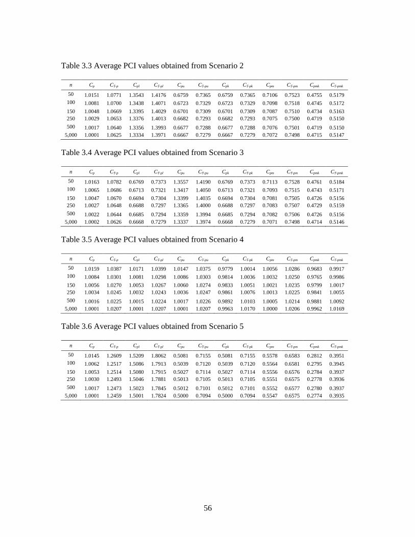
56
Table 3.3 Average PCI values obtained from Scenario 2
n Cp CT-p Cpl CT-pl Cpu CT-pu Cpk CT-pk Cpm CT-pm Cpmk CT-pmk
50 1.0151 1.0771 1.3543 1.4176 0.6759 0.7365 0.6759 0.7365 0.7106 0.7523 0.4755 0.5179
100 1.0081 1.0700 1.3438 1.4071 0.6723 0.7329 0.6723 0.7329 0.7098 0.7518 0.4745 0.5172
150 1.0048 1.0669 1.3395 1.4029 0.6701 0.7309 0.6701 0.7309 0.7087 0.7510 0.4734 0.5163
250 1.0029 1.0653 1.3376 1.4013 0.6682 0.7293 0.6682 0.7293 0.7075 0.7500 0.4719 0.5150
500 1.0017 1.0640 1.3356 1.3993 0.6677 0.7288 0.6677 0.7288 0.7076 0.7501 0.4719 0.5150
5,000 1.0001 1.0625 1.3334 1.3971 0.6667 0.7279 0.6667 0.7279 0.7072 0.7498 0.4715 0.5147
Table 3.4 Average PCI values obtained from Scenario 3
n Cp CT-p Cpl CT-pl Cpu CT-pu Cpk CT-pk Cpm CT-pm Cpmk CT-pmk
50 1.0163 1.0782 0.6769 0.7373 1.3557 1.4190 0.6769 0.7373 0.7113 0.7528 0.4761 0.5184
100 1.0065 1.0686 0.6713 0.7321 1.3417 1.4050 0.6713 0.7321 0.7093 0.7515 0.4743 0.5171
150 1.0047 1.0670 0.6694 0.7304 1.3399 1.4035 0.6694 0.7304 0.7081 0.7505 0.4726 0.5156
250 1.0027 1.0648 0.6688 0.7297 1.3365 1.4000 0.6688 0.7297 0.7083 0.7507 0.4729 0.5159
500 1.0022 1.0644 0.6685 0.7294 1.3359 1.3994 0.6685 0.7294 0.7082 0.7506 0.4726 0.5156
5,000 1.0002 1.0626 0.6668 0.7279 1.3337 1.3974 0.6668 0.7279 0.7071 0.7498 0.4714 0.5146
Table 3.5 Average PCI values obtained from Scenario 4
n Cp CT-p Cpl CT-pl Cpu CT-pu Cpk CT-pk Cpm CT-pm Cpmk CT-pmk
50 1.0159 1.0387 1.0171 1.0399 1.0147 1.0375 0.9779 1.0014 1.0056 1.0286 0.9683 0.9917
100 1.0084 1.0301 1.0081 1.0298 1.0086 1.0303 0.9814 1.0036 1.0032 1.0250 0.9765 0.9986
150 1.0056 1.0270 1.0053 1.0267 1.0060 1.0274 0.9833 1.0051 1.0021 1.0235 0.9799 1.0017
250 1.0034 1.0245 1.0032 1.0243 1.0036 1.0247 0.9861 1.0076 1.0013 1.0225 0.9841 1.0055
500 1.0016 1.0225 1.0015 1.0224 1.0017 1.0226 0.9892 1.0103 1.0005 1.0214 0.9881 1.0092
5,000 1.0001 1.0207 1.0001 1.0207 1.0001 1.0207 0.9963 1.0170 1.0000 1.0206 0.9962 1.0169
Table 3.6 Average PCI values obtained from Scenario 5
n Cp CT-p Cpl CT-pl Cpu CT-pu Cpk CT-pk Cpm CT-pm Cpmk CT-pmk
50 1.0145 1.2609 1.5209 1.8062 0.5081 0.7155 0.5081 0.7155 0.5578 0.6583 0.2812 0.3951
100 1.0062 1.2517 1.5086 1.7913 0.5039 0.7120 0.5039 0.7120 0.5564 0.6581 0.2795 0.3945
150 1.0053 1.2514 1.5080 1.7915 0.5027 0.7114 0.5027 0.7114 0.5556 0.6576 0.2784 0.3937
250 1.0030 1.2493 1.5046 1.7881 0.5013 0.7105 0.5013 0.7105 0.5551 0.6575 0.2778 0.3936
500 1.0017 1.2473 1.5023 1.7845 0.5012 0.7101 0.5012 0.7101 0.5552 0.6577 0.2780 0.3937
5,000 1.0001 1.2459 1.5001 1.7824 0.5000 0.7094 0.5000 0.7094 0.5547 0.6575 0.2774 0.3935

57
Table 3.7 Average PCI values obtained from Scenario 6
n Cp CT-p Cpl CT-pl Cpu CT-pu Cpk CT-pk Cpm CT-pm Cpmk CT-pmk
50 1.0158 1.2629 0.5081 0.7159 1.5236 1.8098 0.5081 0.7159 0.5576 0.6579 0.2806 0.3945
100 1.0080 1.2546 0.5039 0.7125 1.5121 1.7966 0.5039 0.7125 0.5560 0.6576 0.2788 0.3938
150 1.0065 1.2528 0.5032 0.7119 1.5098 1.7938 0.5032 0.7119 0.5558 0.6575 0.2785 0.3936
250 1.0036 1.2495 0.5019 0.7107 1.5053 1.7883 0.5019 0.7107 0.5554 0.6576 0.2781 0.3937
500 1.0020 1.2480 0.5010 0.7101 1.5030 1.7858 0.5010 0.7101 0.5550 0.6575 0.2777 0.3935
5,000 1.0001 1.2460 0.5001 0.7094 1.5002 1.7826 0.5001 0.7094 0.5547 0.6575 0.2774 0.3935
Figure 3.4 Results from Scenario 1 (n = 250)
Figure 3.5 Results from Scenario 2 (n = 250)

58
Figure 3.6 Results from Scenario 3 (n = 250)
Figure 3.7 Results from Scenario 4 (n = 250)
Figure 3.8 Results from Scenario 5 (n = 250)
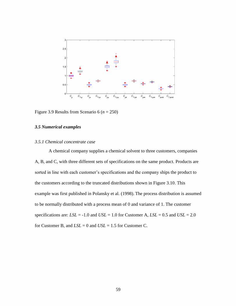
59
Figure 3.9 Results from Scenario 6 (n = 250)
3.5 Numerical examples
3.5.1 Chemical concentrate case
A chemical company supplies a chemical solvent to three customers, companies
A, B, and C, with three different sets of specifications on the same product. Products are
sorted in line with each customer’s specifications and the company ships the product to
the customers according to the truncated distributions shown in Figure 3.10. This
example was first published in Polansky et al. (1998). The process distribution is assumed
to be normally distributed with a process mean of 0 and variance of 1. The customer
specifications are: LSL = -1.0 and USL = 1.0 for Customer A, LSL = 0.5 and USL = 2.0
for Customer B, and LSL = 0 and USL = 1.5 for Customer C.

60
Figure 3.10 Truncated distribution illustrations associated with three customers
For Customer A, given that the LSLA = -1, USLA = 1, A = 0, A =0.54, and
A =0, the truncated mean and variance can be calculated using Equations (3.2) and (3.3),
we get 0T , and 0.3717T . Consequently, the process capability indices are
obtained from Equations (3.4) and (3.6) through (3.9) as follows: 0.8969,T pmC
0.8969,T puC 0.8969,T plC 0.8969,T pkC and 0.8969.T pmkC In repeating the
calculations above, from LSLB = 0.5, USLB = 2, B = 1.04, B = 0.39, and B = 1.25, we
obtain T pmC = 1.6349 and T pmkC = 1.4974 for Customer B; and, with LSLC = 0,
(b) The truncated distribution for customer A (b) The distributions with the specification
limits for each customer
(d) The truncated distribution for customer C (c) The truncated distribution for customer B

61
USLC = 1.5, C = 0.725, C = 0.41, and C = 0.725, we have T pmC = 1.3327 and
T pmkC = 1.2705 for Customer C.
3.5.2 Supplier’s process capability problem
As noted by Asokan and Unnithan (2007), the submitted lot from a vendor for a
supplier problem appears to follow a truncated normal distribution (shown by the
histogram, Figure 3.10). The quality characteristic of interest for this problem is the width
of a particular component, established at 20 2 mm. The average ( )y and standard
deviation of 100 samples is observed to be 20.0876 and 0.9393 mm, respectively.
Figure 3.11 Histogram of the supplier’s submitted lot
The problem specifies that LSL = 18, USL = 22, = 20.0876, =0.9393, and
= 20. To find the PCI values for this study, we start by calculating T and T from
Equations (3.2) and (3.3), followed by the formulations outlined at Equation (3.4) and
Equations (3.6) through (3.9). The resulting measurements obtained are T = 20.07056,
T = 0.8424, T pC = 0.7914, T pkC = 0.7635, T pmC = 0.7886, and T pmkC = 0.7608.

62
3.6 Confidence intervals for the truncated normal PCIs
Confidence intervals (CI) for process capability indices provide an alternative
method for estimating capability, by relaxing the statistical fluctuation that can occur
with various statistical parameters. Another purpose of using the CI for process capability
indices is to evaluate the degree of accuracy in calculations pertaining to a specific
sample size. Since the confidence limit of PCIs may be obtained from estimating only
variance (for Cp), both mean and variance (for Cpk), and the process bias term (for Cpm),
each index needs a unique statistical approximation method, as will be discussed later in
this section. Several closed forms for obtaining the CI of the traditional PCIs have been
proposed from researchers. Kushler and Hurley (1990) suggested a specific method for
evaluating the lower confidence interval of Cp, Cpk, and Cpm. In addition, Chou et al.
(1990) developed lower confidence limits for both Cp and Cpk, Boyles (1991) proposed an
approximate confidence interval for Cpm, and both Johnson and Kotz (1993), as well as
Pearn and Kotz (2006), provided a review of confidence interval estimates for the
traditional indices.
3.6.1 The approximate confidence intervals for T pC
Given that ˆT pC is an estimator for T pC and ˆ ˆ6T p TC USL LSL , where ˆ
T
is the truncated form of the sample standard deviation, it is clear that an estimator for the
standard deviation is the only parameter needed. The quality characteristic Y is assumed
to follow a normal distribution, 1 2, ,..., nY y y y , with mean and standard deviation
, whereby and represent the sample mean and sample standard deviation of Y.

63
Hence, is distributed according to the chi-square distribution, 2
1n , with n-1 degrees of
freedom, for which 2
2 2
1ˆ
1n
n
.
From Equation (3.3) in Section 3.3.3, we have that 2 2
T t , where t is a
constant term,
2
1Φ Φ Φ Φ
l l u u l u
u l u l
z z z z z z
z z z zt
, and2ˆT is assumed to follow a
chi-square distribution; hence, 2
2 2
1ˆ
1T n
t
n
.
To estimate the confidence interval for ˆT pC , from
ˆ ˆ
ˆT p
T p
C t
tC
, we have that
2
1 2
1P P
ˆT p
n
T p
C nc
cC
. With 2 2
1 1,P n n , we can obtain the confidence
interval for 2 from 2 2
2 2 2
1, 2 1,1 2ˆP 1
1 1n n
n n
, or
2 2
2
2 2
1,1 2 1, 2
ˆ ˆ1 1P 1
n n
n n
(3.10)
When multiplying the inverse of the constant term for ˆT pC in Equation (3.10), we have
2 2
1,1 2 1, 2
6 1 6 6 1ˆ ˆ ˆP 1
n n
n nt t t
USL LSL USL LSL USL LSL
(3.11)
2 2
1,1 2 1, 2P 1
ˆ ˆ ˆ6 1 6 6 1
n n
T T T
USL LSL USL LSL USL LSL
n n

64
2 2
1,1 2 1, 2ˆ ˆP 11 1
n n
T p T p T pC C Cn n
Finally, the100(1 )% confidence interval for ˆT pC is derived as
2 2
1, /2 1,1 /2ˆ ˆ,1 1
n n
T p T pC Cn n
(3.12)
If the desired percentage is not found in the standard chi-square table, the Wilson-
Hilferty method introduced by Johnson and Kotz (1970) can be used to approximate the
chi-square percentile point, which is expressed as
31
22
,1 1
2 21
9 9z
, (3.13)
where represents the degrees of freedom for the chi-square, and z is the upper quartile
of the standard normal distribution. If the sample size is less than ten, it is noted that this
approximation may not offer a suitable level of precision.
By substituting formulation (3.13) in (3.12), the 100(1 )% confidence intervals
for ˆT pC is derived as
3 31 12 22 2
2 1 2
2 2 2 2ˆ ˆ1 19 1 9 1 9 1 9 1
,T p T pC z C zn n n n
(3.14)

65
3.6.2 The approximate confidence intervals for T pkC
Estimating the confidence interval for T pkC involves not only the variance, but
the mean as well. While several distributions have been suggested previously by
researchers, such as the folded normal distribution, t distribution, or chi-square
distribution, the most prevalent method is to use the normal distribution. The distribution
is first reported in use by Zhang et al. (1990) for confidence interval estimation, with
major modifications proposed by Kusher and Hurley (1992), and Nagata and Nagahata
(1993).
For a normally distributed process with a large sample size, i.e., kn > 30, where k
is the subgroup size and n is the sample size of each sub group, ˆT pkC can be estimated
using the Bissell method outlined by Bissell (1990). This particular method was shown
by Kushler and Hurley (1992) to outperform other approaches when n is large.
Using the general form, min ,3 3
T TT pk
T T
USL USLC
, we use the
coefficient of variation for T pkC , CV( T pkC ) to estimate ˆT pkC , which is defined as
3
TT pk
T
USLCV C CV
or
3
TN
TN
USLCV
.
From the Taylor series expansion, it follows that 2 2
( ) ( ) ( )CV a CV b CV c , where
/a b c (see Stuart and Ord, 1987). Hence,
2 2ˆ ˆ ˆ( ) ( ) (3 )T pk T TCV C CV USL CV (3.15)

66
From
22
2 2 2 2
ˆ ˆ ˆ 1ˆ( )
ˆ9ˆ ˆˆ
T T
T
T pkT TT
Var USL VarCV USL
knCUSL kn USLE USL
and
22
2 2
ˆ ˆ(3 ) 9 1ˆ(3 )
ˆ2 1 9 2 1ˆ3
T TT
TT
VarCV
k n k nE
, Equation (3.15) becomes
2
1 1ˆ( )ˆ 2 19
T pk
T pk
CV Ck nknC
The standard error of ˆT pkC , ˆ( )T pkSE C , is obtained by multiplying ˆ
T pkC and ˆ( )T pkCV C .
As a result, we get
2
2
ˆ1 1 1ˆ ˆ( )ˆ 2 1 9 2 19
T pk
T pk T pk
T pk
CSE C C
k n kn k nknC
When n is large, i.e., n > 30, the term 1
9knapproaches zero, thus, with one
subgroup (k = 1), ˆ( )T pkSE C becomes
2ˆˆ( )
2 1
T pk
T pk
CSE C
n
. Finally, the approximate
100(1 )% confidence interval for T pkC is derived as
2 2
2 2
ˆ ˆˆ ˆ,
2 1 2 1
T pk T pk
T pk T pk
C CC z C z
n n
, which can be further written as
2 2ˆ ˆ1 , 12 2 2 2
T pk T pk
z zC C
n n
(3.16)
3.6.3 The approximate confidence intervals for T pmC
With
2 22 26 6
T pm
T T
USL LSL USL LSLC
t t
,

67
we have
2
2
T pm
dC
t t
, where( )
6
USL LSLd
.
Therefore,
2 22 2
( 1)ˆ ˆ
ˆT pm
d d
nt t t
C
s t yn
,
where 2
1
1n
i
i
s y y n
.
The process bias term, 2
1
( )n
i
y
, can be estimated from 2
1
22( )n
i
E y
;
see Taguchi (1985). As reported in Boyles (1991), Pearn et al. (1992), Vannman and
Kotz (1995), and Zimmer et al. (2001), it is generally known that the bias term follows a
non-central chi-square distribution, 2 2
,n , with n degrees of freedom and the non-
centrality parameter, .
Given that 2
2 2t t , we have 2
2
,
2ˆ
n
n
t
, thus
2
22,
ˆn
t n
. See
Johnson and Kotz (1970) for the proof.
Hence, with
22
22
T pm
dC
t t
, we have
22
2
ˆ ˆ
T pm
d
C
,
22
22
1T pm
dt
C n
,
and
2 22 22 2
2 22 2
ˆ 1 1
ˆ ˆT pm T pm
T pm T pm
C n Cd
t d nC C
.

68
Thus, with
2 22
2 1T pm
dC
n t
, we have that
22 2,
2 2 2
ˆ
ˆn
T pm
d
C t nt
, or
22
2 2
,
ˆT pm
n
dC
t
n
. Finally, we get the cumulative density function of ˆT pmC as
2
,
ˆT pm
n
dC
n
t , where
2t
nt
and from
2
ˆ1 ,
ˆT pmC
, where
22
2
ˆ1
ˆˆ
ˆ1 2
ˆ
tn
t
t
t
. See Patniak (1949).
To approximate the 100(1 )% lower confidence bound for T pmC , we have
2 2
1 2, , 2, ,
ˆ1 1 1T pm T pm T pm
n n
n nP C C C
n n
Let 2
1 2, ,
1L
T pm T pm
n
nC C
n
be the lower confidence limit and
2
2, ,
1U
T pm T pm
n
nC C
n
be the upper confidence limit, then
1L U
T pm T pm T pmP C C C
2 2 2
ˆ ˆ ˆ 1ˆ ˆ ˆ
L U
T pm T pm T pm
T pm T pm T pm
C C CP
C C C
2
2
,
2
ˆˆ ˆ 1
ˆ ˆ
L U
T pm T pm
T pm T p
n
m
C CP
C C

69
Since 2
ˆ, ,n is the 100(1 )% lower confidence interval for 2
ˆ,n , the previous equation
yields
2 2
2, , 1 2, ,ˆ ˆˆ ˆ ˆ 1ˆ ˆ
T pm T pm T
n n
pmP C C C
Finally, the 100(1 )% interval approximation for CT-pm is written as
2 2
2, , 1 2, ,ˆ ˆˆ ˆ,ˆ ˆ
T pm T p
n n
mC C
, where
22
2
ˆ1
ˆˆ
ˆ1 2
ˆ
T
T
T
T
n
(3.17)
Equation (3.17) is similar to Equation (3.12), yet in this case, the non-central parameter is
added to the calculation. Thus, by using Equation (3.13) and lettingˆ
ˆT
d
T
t
, we then
obtain the form of the approximation in Equation (3.18) as
3 3
2 22 2 2 2
1 2 22 2 2 22 2 2 2
2 1 2 2 1 2 2 1 2 2 1 2ˆ ˆ1 , 1
9 1 9 1 9 1 9 1
d d d d
T pm T pm
d d d d
t t t tC z C z
n t n t n t n t
(3.18)
3.6.4 The approximate confidence intervals for T pmkC
The index, T pmkC , is a combined function of T pkC and T pmC . Hence, from
Sections 3.6.2 and 3.6.3, a natural estimator of T pmkC is distributed as a mixture of the
chi-square and the non-central chi-square distribution. In this section, the approximate
confidence interval of ˆT pmkC will be modified from a derivation provided by previous

70
researchers. In particular, Chen and Hsu (1995) derived the sampling distribution of Cpmk
and reported that ˆpmkC is asymptotically normal and consistent if the fourth moment of Y
is finite. Therefore, under similar circumstances, since we will assume that ˆT pmkC is
distributed by a truncated normal distribution, the confidence interval is estimated by
considering the variance of ˆT pmkC at a certain confidence level from the standard normal
distribution.
Staring with min ,3 3
T TT pk
T T
USL USLC
, and using the formula
1 12 2
min ,x y x y x y , we obtain
1 1
2 3 3 2 3 3
T T T TT pk
T T T T
USL USL USL USLC
Thus. ( ) 2
6
T
T pk
T
USL LSL USL LSLC
. From
2
1
T pk
T pmk
T
T
CC
, we get
22
( ) 2
6
T
T T
T pmk
USL LSL USLC
LSL
.Similarly, the estimator for T pmkC is
22
ˆ(ˆ
ˆ
) 2
ˆ6T k
T
pm
T
T
USL LSL US LSLC
L
. If the mean is centered at the midpoint
between the specification limits,2
USL LSL
, then we have ˆ ˆ
T pmk T pmC C , so that
ˆT pmkC can be estimated using Equation (3.18). Otherwise, the 100(1 )% interval
approximation for ˆT pmkC is obtained as

71
2 2
ˆ ˆˆ ˆ,
T pmk T pmk
T pmk T pmkC z C zn n
(3.19)
where 2z is the upper 2 quartile of the standard normal distribution, and 2ˆT pmk is the
asymptotic estimator of ˆ( )T pmkVar C , which is formulated as
32
2 4
4
2 2
22 22
24 11 2ˆ ˆˆ
9 1 24 13 1
T
T pmk T pmk T pmk
md
C C
(3.20)
where ( )
6
USL LSLd
,
4
4
1
ˆT
ni
i
ym
n
, and
ˆ
ˆT
T
. See the full derivation of
ˆpmkC in Pearn et al. (1992) and Chen and Hsu (1995).
3.7 Numerical examples of confidence intervals for proposed posterior PCIs
Given that n = 30, [LSL, USL] = [-3, 3], = 0.05, ˆT = 1, ˆ
T = 0, and = 0, the
confidence intervals of the posterior PCIs are shown as follows. Using Equation (3.13),
the estimated 95% confidence interval for ˆ 1.0T pC is obtained as
ˆ0.7439 1.2556T pC . The estimated 95% confidence interval for ˆ 1.0T pkC is
computed as ˆ0.7426 1.2574T pkC using Equation (3.15). Similarly, the estimated
confidence interval of ˆT pmC is obtained from Equation (3.17). With ˆ ˆ 0d T Tt ,
the 95% confidence interval of ˆ 1.0T pmC is then ˆ0.7481 1.2514T pmC . Finally,
the asymptotic 95% confidence interval for ˆT pmkC is computed using Equation (3.19).

72
Prior to using Equation (3.19), the 2ˆT pmk need to be obtained from Equation (3.20).
Assuming 41, 0,d m and 0 , we then have2ˆ 0.0694T pmk . Using Equation
(3.19), the confidence interval of ˆ 1.0T pmkC then yields ˆ0.9057 1.0943 .T pmkC
The estimated confidence intervals of the proposed posterior PCIs with different sample
size n and different confidence level are presented in Table 3.8 and Figure 3.12, where
the wider confidence intervals are observed as sample size or the confidence level
decreases.
3.8 Concluding remarks
In summary, this chapter proposes a new set of posterior process capability
indices for the situations where the underlying process follows a truncated normal
distribution and a target-based framework is desired. The simulation results demonstrate
that the proposed posterior indices have higher index values, compared to traditional PCI
values. This is because smaller process variances are transmitted to the customer after
implementing specifications on a process. As a result, a significant degree of difference
may result from using traditional PCIs on processes where the observations clearly follow
a truncated normal distribution which is the actual process distribution transmitted to the
customers. The purpose of this chapter is twofold. First, the proposed customer-based
posterior PCIs are derived and compared with traditional manufacturer-based PCIs. The
confidence interval is a prominent tool providing an interval estimation of PCIs designed
to increase the versatility of the process capability analysis. Accordingly, the confidence
intervals for the proposed posterior PCIs are also developed.

73
Table 3.8 Confidence intervals of the proposed PCIs under different settings
ˆT pC
n ˆLower T pC ˆUpper T pC
ˆT pC
n ˆLower T pC ˆUpper T pC
1.0 10 0.05 0.5478 1.4538 1.0 30 0.1 0.7814 1.2114
1.0 20 0.05 0.6847 1.3149 1.0 30 0.05 0.7439 1.2556
1.0 30 0.05 0.7439 1.2556 1.0 30 0.025 0.7110 1.2955
1.0 50 0.05 0.8025 1.1971 1.0 30 0.010 0.6726 1.3434
1.0 100 0.05 0.8608 1.1389 1.0 30 0.005 0.6467 1.3767
1.0 250 0.05 0.9122 1.0877 1.0 30 0.0025 0.6228 1.4081
1.0 500 0.05 0.9380 1.0620
1.0 30 0.0010 0.5938 1.4472
ˆT pkC
n ˆLower T pkC ˆUpper T pkC
ˆT pkC
n ˆLower T pkC ˆUpper T pkC
1.0 10 0.05 0.5380 1.4620 1.0 30 0.1 0.7840 1.2160
1.0 20 0.05 0.6821 1.3179 1.0 30 0.05 0.7426 1.2574
1.0 30 0.05 0.7426 1.2574 1.0 30 0.025 0.7057 1.2943
1.0 50 0.05 0.8020 1.1980 1.0 30 0.010 0.6618 1.3382
1.0 100 0.05 0.8607 1.1393 1.0 30 0.005 0.6314 1.3686
1.0 250 0.05 0.9122 1.0878 1.0 30 0.0025 0.6030 1.3970
1.0 500 0.05 0.9380 1.0620 1.0 30 0.0010 0.5679 1.4321
ˆT pmC
n ˆLower T pmC ˆUpper T pmC
ˆT pmC
n ˆLower T pmC ˆUpper T pmC
1.0 10 0.05 0.5698 1.4312 1.0 30 0.1 0.8141 1.1807
1.0 20 0.05 0.6925 1.3071 1.0 30 0.05 0.7816 1.2180
1.0 30 0.05 0.7481 1.2514 1.0 30 0.025 0.7529 1.2516
1.0 50 0.05 0.8045 1.1952 1.0 30 0.010 0.7195 1.2920
1.0 100 0.05 0.8615 1.1382 1.0 30 0.005 0.6967 1.3200
1.0 250 0.05 0.9124 1.0875 1.0 30 0.0025 0.6757 1.3464
1.0 500 0.05 0.9380 1.0619
1.0 30 0.0010 0.6501 1.3793
ˆT pmkC
n ˆLower T pmkC ˆUpper T pmkC
ˆT pmkC
n ˆLower T pmkC ˆUpper T pmkC
1.0 10 0.05 0.8367 1.1633 1.0 30 0.1 0.9209 1.0791
1.0 20 0.05 0.8845 1.1155 1.0 30 0.05 0.9057 1.0943
1.0 30 0.05 0.9057 1.0943 1.0 30 0.025 0.8922 1.1078
1.0 50 0.05 0.9270 1.0730 1.0 30 0.010 0.8761 1.1239
1.0 100 0.05 0.9484 1.0516 1.0 30 0.005 0.8649 1.1351
1.0 250 0.05 0.9673 1.0327 1.0 30 0.0025 0.8545 1.1455
1.0 500 0.05 0.9769 1.0231 1.0 30 0.0010 0.8417 1.1583

74
Figure 3.12 Estimated confidence intervals of the proposed posterior PCIs under various
sample sizes (left) and various levels of type I error (right)

75
CHAPTER 4
ROBUST PARAMETER DESIGN OPTIMIZATION AND
PROCESS CAPABILITY ANALYSIS FOR TYPE I-RIGHT CENSORED DATA
4.1 Introduction
Continuous process improvement is critical in maintaining a competitive
advantage in the marketplace. It is also recognized that process improvement activities
are most efficient and cost-effective when implemented during the early design stage.
Based on this awareness, robust parameter design (RPD) was introduced as a systematic
method for applying experimental design and optimization tools. The primary goal of
RPD is to determine the best design factor settings, or the optimum operating conditions,
that minimize performance variability and deviations from the target value of a product.
Because of their practicability in reducing the inherent uncertainty associated with system
performance, the widespread application of RPD techniques has resulted in significant
improvements in product quality, manufacturability, and reliability at low cost (see
Robinson et al., 2004, Jen, 2005, Hasenkamp et al., 2009, and Montgomery, 2013).
Although a number of RPD methods have been developed, there is still ample room for
improvement, particularly when censored data are under study. This chapter aims to
develop new RDP methodologies that can be applied in survival analysis and reliability
studies where censored data are common. In this section, applications of RPD that have
not been widely explored by the research community are discussed, and specific
objectives of this chapter are outlined.

76
4.1.1 Current research gaps and research objectives
The main purpose of this chapter is twofold. We first develop a series of RPD-
based methodological models for a time-oriented quality characteristic, coupled with type
I-right censoring. We then propose various RPD optimization models to determine the
optimum operating conditions that maximize survival times and minimize proportional
hazards in conjunction with variability. The specific goals of this chapter with supporting
rationales are as follows.
Static non-time oriented quality characteristics have been the main focus in
traditional RPD studies, even though time-oriented quality characteristics routinely
appears in many engineering problems, particularly in survival analysis and reliability
studies. The term survival analysis refers to statistical inferences for time-related data
with censoring. A survival data set contains observations within a predetermined time or
restricted values. On the other hand, unmeasured data outside the restricted time range or
values are called censored data. By definition, censoring is a form of incomplete data
similar to data truncation. In truncation, any data beyond the truncation points is
neglected. However, for censoring, any data beyond the censoring points are censored but
are still included in the study, although its actual value is unknown. For instance,
censored observations t that survive longer than censoring time tc (i.e., ct t ) are entered
as tc. Therefore, the distribution of this incomplete data set is said to follow a censored
distribution (see Cohen, 1991). There are four main types of censoring mechanisms: left
censoring, right censoring, interval censoring, and progressive censoring. In addition,
there are two types of censoring. Type I-censoring is a scheme based on a specific time,

77
and time-censored experiments take place when a test is terminated at a pre-specified
time; hence, the number of data points censored is a random variable. In contrast, the
basis of type II-censoring is a fixed number of data points being censored, and the
censoring threshold becomes a random variable. While each censoring type has its own
set of statistical foundations, type I-right censoring is the most common methodology in
reliability studies. Despite the potential application areas and practical needs, there is
little research work on the censoring-based RPD modeling and optimization. As such,
this chapter develops detailed guidelines for the design of a new RPD with the
consideration of type I-right censoring concepts.
It is expected that incorporating considerations for reliability in the early stages of
production design leads to a higher level of product quality over time and less costs due
to product recalls. However, little research has been done on how to achieve this when
optimizing process parameters. The survival time used in reliability studies is restricted to
be positive and often has a skewed distribution. In contrast, the standard statistical
methods of the traditional RPD rely on the normal distribution, which may be unsuitable
to fit the survival time into such models. As a result, the connection between the survival
time and RPD requires further methodological developments. To this end, we propose the
censoring-based RPD methods for assessing the optimum operating conditions using the
response surface methodology. In addition, special methods that can estimate failure rates
with censored data, such as the hazard function, the Kaplan-Meier (KM) estimator, and
the maximum likelihood estimation, are routinely used for regression in survival analysis.
However, the statistical inferences for survival time can be developed parametrically or

78
non-parametrically. Since the distribution of survival time is typically unknown prior to
the actual data collection, nonparametric estimation methods for survival time are often
preferred over the parametric counterpart. In particular, hazard functions, accompanied
with median survival functions, may provide more insights into a failure mechanism.
More specifically, survival times are often highly skewed, and the median is generally
considered a better measure of central location than the mean. While the median survival
function represents the survival probability of a subject at time t, the hazard function
indicates the risk of failure of the subject at time t. The proportion of hazard rates, called
a hazard ratio or proportional hazards, is useful in this particular research context. For a
predicted response surface model, the semiparametric Cox proportional hazards (PH)
regression model is often employed, as outlined in the literature review section. Thus,
another purpose of this chapter is to propose a new set of response-surface-based
optimization models by incorporating the nonparametric methods, such as the Cox PH
model and the KM estimator, to investigate the effect of input variables under the
type I-right censoring scheme.
4.1.2 Literature review
Traditionally, RPD and survival analysis have been treated as separate fields with
no significant connections to each other. Previous works in those areas are abundant, but
virtually no research work on potential links between the two fields has been reported. In
this section, some key papers that are potentially aligned with this study are included.
The basic concepts of RPD were introduced by Taguchi (1986) and have been
successfully used as an efficient tool for building quality into the design of processes to

79
improve the quality of products. The main purpose of the RPD is to minimize variability
in the output response of a product around the target value. The comprehensive
discussion of Taguchi’s RPD concepts and tools was examined by Nair et al. (1992),
Robinson et al. (2003), and Park et al. (2006). Vining and Myers (1990) were among the
first to offer the response-surface-based RPD as an alternative approach for modeling
process relationships. They used a well-established statistical method, the response
surface methodology, while incorporating basic principles of Taguchi’s original version
of RPD that include minimizing process variability and deviations from the target value.
Along those lines, Del Castillo and Montgomery (1993) proposed the use of the
generalized reduced gradient method as an optimization technique in order to obtain RPD
solutions more efficiently. Lin and Tu (1995) then showed that the RPD solutions
obtained from the aforementioned models might potentially eliminate better solutions
from consideration, since their models strictly force the process mean to be located at a
specific target value. Accordingly, they used the mean squared error (MSE) model to
include a bias allowance based on the deviations between the process mean and the target
value. The tradeoff in balancing bias and variability is a significant research issue. Based
on this awareness, Cho et al. (2000) conducted further modifications of the MSE model
by incorporating priority concepts and developed a nonlinear goal programming RPD
model. In addition, Kim and Cho (2002) introduced a priority-based preemptive RPD
model.
Special optimization methods are necessary to optimize the multiple response
processes when there are multiple quality characteristics under study. For instance,

80
Kovach and Cho (2009), He et al. (2012), Goethals and Cho (2012), and Brito et al.
(2014) proposed various multi-criteria optimization models for studying tradeoffs in RPD
problems. Also, Shin and Cho (2005) proposed a bias-specified bi-objective RPD model
as a relaxed zero-bias approach while keeping variability at the minimum. As an
extension, Shaibu and Cho (2009) proposed an RPD model by incorporating a higher-
order polynomial function. Another challenge in solving RPD problems is that part of the
data is often missing when conducting experiments. Cho and Park (2005) developed RPD
models using the iterative expectation maximization algorithm when the data is
unbalanced. Other RPD articles written by Hu et al. (2014), Fang et al. (2015), Bao et al.
(2016), Brito et al. (2016), and Ouyang et al. (2016) illustrated a wide spectrum of
application areas of RPD, including the hydrokinetic turbine system, the fatigue life of a
product, and machine parts. Finally, there are many practical situations where some of the
input variables are constrained to be integer values. Ozdemir and Cho (2016, 2017)
developed mixed nonlinear integer programming RPD models and numerically solved the
Karush-Khun-Tucker system of equations.
Survival time and hazard functions are well developed in the area of survival
analysis (see Kleinbaum and Klein, 2006, and Kalbfleisch and Prentice, 2011).
A few authors studied how to maximize the survivability using regression functions in
the medical research (see Mead and Pike (1975) and Carter and Wamper (1986)).
In particular, Carter et al. (1979) proposed a regression model using a hazard function to
estimate drug interactions from chemotherapy experiments. In addition, Solana et al.
(1987) evaluated biological interactions of three genotoxic agents by maximizing the

81
median survival time using a polynomial regression. Das (2009) also proposed a
regression model for handling survival data using a modified least squares estimator,
assuming that the data follows a Weibull distribution. Similarly, Kuhn et al. (2000) used
regression models to find an optimal combination of two drugs that maximizes survival
time of patients in tumor studies and used the maximum likelihood estimator to estimate
the mean and variance of experimental data. On the other hand, Shaibu et al. (2009)
proposed new optimization models for censored data and obtained optimal factor settings
using the expectation maximization method. Finally, Li et al. (2012a, 2012b, 2013)
developed censoring-embedded nonlinear optimization models to find the optimal
formulations for new tablet drugs in dissolution and bioequivalence studies.
4.2 Model development
This study consists of three sequential phases: experimentation, estimation, and
optimization. In Section 4.2.1, the modified central composite design (CCD) for type I-
right censored data is developed since the experimental design schemes that are currently
available may not be effective in handling censored data. Based on the proposed CCD,
Section 4.2.2 develops the survival distribution to estimate the median survival time and
standard error of the median survival time, followed by their fitted functions in Section
4.2.3. In parallel with the fitted functions for median survival time and standard error of
the median survival time based on the KM estimator, the fitted function for proportional
hazards rate using the Cox proportional hazards model is developed in Section 4.2.4.
Based on the fitted functions developed in Sections 4.2.3 and 4.2.4, various RPD
optimization models are proposed in Section 4.3, followed by the numerical examples in

82
Sections 4.4.1, 4.4.2, and 4.4.3, where optimum operating conditions are compared.
Based on the numerical results, Section 4.5 presents additional insights on the advantage
of the nonparametric KM estimator over the maximum likelihood estimator using other
parametric distributions. Finally, conclusions and future studies are discussed in Section
4.6. The structure of the research is depicted in Figure 4.1.
4.2.1 Development of the modified central composite design under the type I-right
censoring scheme
For many production processes, a model that incorporates linear and quadratic
effects of input variables on the response variable of interest is often required to
approximate the response (see Montgomery, 2013). The central composite design (CCD),
developed by Box and Wilson (1951), is a useful design of experiments for building the
second-order model for the input variables. The CCD is partitioned into three sets of
design points, which are factorial points to estimate linear and interactions effects, axial
points to capture curvature effects and maintain the design rotatability, and center points
to maintain the orthogonality of a design with the parameters minimally correlated to
each other. The CCD is rotatable in the sense that all equidistant points from the center
point in any direction have approximately the same variance in prediction.
This rotatability is achieved by setting the axial points, , equal to 1/4
,fn where fn
represents the number of factorial points. The rotatability is a crucial design property
because the optimum operating conditions determined through the CCD can maximize
process yield in a consistent manner, particularly when making prototyping decisions
about process models in the early stages of industrial research and development.

83
Under the type I-right censoring scheme, the traditional CCD needs to be
modified for two reasons. First, when the data is censored, we assume that there are two
types of observations: the actual survival time of a unit (i.e., uncensored survival time)
and the survival time at the termination time of an experimental period (i.e., censored
survival time). Let T denote the matrix of the observed survival times from r
experimental runs with n units in the ith run where ijt T , 1,...,i r , and 1,...,j n .
Then, each recorded survival time ijt is determined as follows:
for and
for and
ij ij c
ij
c ij c
t t t i jt
t t t i j
where ijt T , T is an r n matrix of recorded survival times, ct is the termination time,
known as censoring time, and 0 and ijt i j . Second, to appropriately estimate the
statistical descriptions of the recorded survival data at each design point, the traditional
statistical estimators used in CCD (i.e., the mean and the variance of the normal
distribution) are then replaced with two survival analysis-based nonparametric estimators.
These include the median survival time and the variance of the median survival time. As
such, the erroneous results from assuming an improper underlying distribution of the
recorded survival time can be prevented; see Section 4.5. Table 4.1 portrays the modified
rotatable CCD in coded levels, along with center point replications, under the type I-right
censoring scheme.
84
Section 4.2.1
Develop the central composite design
for type I-right censoring
Section 4.2.2
- Develop survival distribution using
nonparametric estimator
- Derive median survival time (M)
- Derive standard error of median
survival time, SE(M)
Section 4.2.3
Develop fitted function for M(x) and
SE[M(x)] using multiple linear
regression
Section 4.2.4
Develop fitted function for hazard
rate, H(x), using Cox proportional
hazard regression
Section 4.3
Develop RPD optimization models
- Three schemes; Scheme I: Minimizing hazard rate; Scheme II: Maximizing
survival time; Scheme III: Minimizing variation
- Three tiers within each scheme; Tier I: single constraint; Tier II:
dual constriants; Tier III: triple constraints.
Phase I:
Experimentation
Phase II:
Estimation
Phase III:
Optimization
Section 4.4.1
- Develop survival distribution
- Estimate M and SE(M)
- Obtain fitted function for M(x) and
SE[M(x)]
Section 4.4
Present numerical example from
pharmaceutical field
Section 4.4.2
- Develop initial fitted function for H(x)
- Check the proportional hazard (PH)
assumption
- Revise the fitted function for H(x)
until the PH assumption is satisfied
Section 4.4.3
- Run the optimization models
based on twelve combinations of
M(x), SE[M(x)] and H(x)
- Discuss and summarize the
optimization results
Section 4.5
Discuss advantages of using
nonparametric estimator
for type I-right censored data
Section 4.1
- Introduction
- Research goals and motivations
- Literature review
Section 4.7
Conclude the chapter
Robust parameter design
Section 4.6
Develop process capability index
for type I-right censored data
Figure 4.1 Structure of Chapter 4
Table 4.1 Experimental format for the modified central composite design for censored
and uncensored data under the type I-right censoring scheme
Input variables Observations M SE(M)
1x 2x … kx
Factorial
points -1 -1 … -1 11t 12t … int 1m 1( )SE m
1 -1 … -1 21t 22t … 2nt 2m 2( )SE m
1 1 … 1
Axial
points
0 … 0 0 … 0
0 … 0
0 … 0
0 0 …
0 0 …
Center
points
0 0 … 0
0 0 … 0
0 0 … 0 1rt 2rt … rnt rm ( )rSE m

85
4.2.2 Development of the fitted functions for median survival time and variance of
the median survival time
4.2.2.1 Construction of the survival distribution for type I-right censored samples
A survival distribution is a probability distribution that links each outcome of an
experiment to its probability of being survived. In this chapter, the Kaplan-Meier (KM)
estimator developed by Kaplan and Meier (1958), one of the most-widely used
nonparametric estimators for evaluating survival times with right censoring, is used.
Initially, the observations in the experimental run i are ranked in increasing order; thus,
we have 1 andij ijt t i j . The survival distribution, also known as a survival curve, at the
ith design point consists of survival functions, ( ) .ijS t j Note that the survival function
shows the probability that a unit survives longer than time ijt and T denotes the random
variable of observed survival times. Since the units that survive at time ijt (i.e., ijT t )
also survive at the time 1ijt (i.e., 1ijT t ), the survival function ( )ijS t is estimated from
the joint probability density function of ijT t and 1ijT t . Thus, it can be defined as
1 1 1( ) ( , ) ( | ) ( ).ij ij ij ij ij ijS t P T t T t P T t T t P T t Consequently, we have
1 1 2 2 3
2 1 1
( | ) ( | ) ( | )( )
( | ) ( | 0) ( 0)
ij ij ij ij ij ij
ij
i i i
P T t T t P T t T t P T t T tS t
P T t T t P T t T P T
Suppose that ijn is the number of units at risk at time ijt and ijd is the censoring indicator
associated with ijt where 0, for ; 1, for ij ij c ij ijd t t t t . The conditional probability

86
function 1( | )ij ijP T t T t is then estimated as 1( | )ij ij
ij ij
ij
n dP T t T t
n
and
( 0) 1P T . Therefore, the estimated survival function at time ijt is obtained as
1 1
( ) 1 ,j j
i i iij
i i
n d dS t
n n
(4.1)
where 0 ( ) 1ijS t and ( 0) 1.ijS t Note that if the survival time is censored 0ijd ,
we obtain 1( ) ( ).ij ijS t S t As a result, ( )ijS t j can be plotted versus ijt j to show the
survival curve of the ith design point. An illustrative plot is shown in the numerical
example section.
4.2.2.2 Estimation of the median survival time and the variance of the median survival
time
To find the central value of the survival data and the variation of the central value,
the median is used because it is more effective in capturing the characteristics of a
skewed distribution that is often found in censored data. For details, see Kaplan and
Meier (1958), and Lee and Wang (2003). The median is, by definition, the 50th percentile
of the distribution, or the largest data point ijt such that ( ) 0.5.ijS t Therefore, the
estimated median survival time of experimental observations of the ith design point, im ,
is obtained as
max | ( ) 0.5i ij ijm t S t i (4.2)
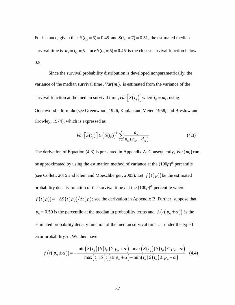
87
For instance, given that 3( 5) 0.45iS t and
4( 7) 0.51iS t , the estimated median
survival time is 3 5i im t since 3
ˆ( 5) 0.45iS t is the closest survival function below
0.5.
Since the survival probability distribution is developed nonparametrically, the
variance of the median survival time , ( ),iVar m is estimated from the variance of the
survival function at the median survival time , ijVar S t
where ij it m , using
Greenwood’s formula (see Greenwood, 1926, Kaplan and Meier, 1958, and Breslow and
Crowley, 1974), which is expressed as
2
1
( ) ( )j
iij ij
i i i
dVar S t S t
n n d
(4.3)
The derivation of Equation (4.3) is presented in Appendix A. Consequently, iVar m can
be approximated by using the estimation method of variance at the (100p)th percentile
(see Collett, 2015 and Klein and Moeschberger, 2005). Let f t p be the estimated
probability density function of the survival time t at the (100p)th percentile where
f t p S t p t p ; see the derivation in Appendix B. Further, suppose that
mp = 0.50 is the percentile at the median in probability terms and i mf t p is the
estimated probability density function of the median survival time im under the type I
error probability . We then have
min | max |
max | min |
ij ij m ij ij m
i m
ij ij m ij ij m
S t S t p S t S t pf t p
t S t p t S t p
(4.4)

88
Finally, the variance of the median survival time of at the design point ith is obtained as
2
[ ]i
i
i m
Var S mVar m
f t p
(4.5)
where [ ]iVar S m is obtained from Equation (4.3), i.e., .ij it m Similarly, the standard
error of the median survival time, ,iSE m is written as
2
[ ]( )
i
i
i m
Var S mSE m
f t p
(4.6)
4.2.3 Estimation of fitted functions for median survival times and variance of
median survival times
The fitted function, known as the response surface function, is a statistical model
for estimating the relationship between input variables and their responses, which serves
as a bridge between the experimentation phase and the optimization phase of RPD. The
fitted function for a curvature is generally obtained using the multiple linear regression,
which is defined as y Xβ e , where
1
2
r
y
y
y
y ,
11 12 1
21 22 2
1 2
1
1
1
k
k
r r rk
x x x
x x x
x x x
X ,
0
1
k
β ,
and 1 2 .T
re e ee Note that y is an 1r vector of responses; X is an r k
vector of design matrix of k regression parameters; β is a 1k vector of regression
coefficient; and e is an 1r vector of random errors, where ˆ e y y . Using the least
squares method, the vector of least squares estimates,b , is then obtained from
1( )b X'X X'y . Therefore, ˆ y Xb . Letting M be a vector of the estimated median

89
survival time where 1 2 ,r
Tm m mM the fitted function of the median survival
time is estimated as
ˆMM x Xb (4.7)
where1( )M
b X'X X'M . In a similar manner, the fitted function for the standard error of
the median survival time is then obtained as
ˆ ˆSSE M
x Xb , (4.8)
where 1( )S
b X'X X'S and S is a vector of the estimated standard error of the median
survival time, 1 2 .T
rSE m SE m SE m S
4.2.4 Development of fitted function for proportional hazards using the Cox
proportional hazards regression
In parallel with the fitted functions for median survival times and variance of
median survival times as shown in Section 4.2.3, the fitted functions for proportional
hazards rate are developed in this section. In order to strengthen the traditional RPD
optimization model, one of this study’s contributions is to incorporate the proportional
hazards rate as an additional measure of the product’s lifetime. Unlike the median
survival time and its variance, the proportional hazards rate give better insights on the
failure risk of a unit, which is known as the mortality rate in the medical research. To
estimate the functional relationship between the input variables and their proportional
hazards rate, the Cox proportional hazards (PH) model (Cox and Oakes, 1972) is
recommended since it does not require the assumption of the underlying distribution of

90
censored data. This section presents the definition of the proportional hazards, as well as,
a brief background of the Cox PH model.
The hazard rate ( )h t represents another perspective of survivability, and it is
defined as the risk (or probability) that an observed unit fails within [t, t + t ] with
0t , or
0( ) lim .
t
P t T t th t
t P T t
Denoting ( )f t and ( )F t as a probability density
function and a cumulative density function of survival time T respectively, we have
0
( ) ( )( ) lim
t
F t t F tf t
t
,
0
( ) ( )
t
F t f u du , and S t P T t where ( ) 1 ( ).S t F t
The hazard rate is then defined as 0
( ) ( )( ) lim
t
F t t F th t
t S t
, yielding
( )( )
( )
f th t
S t .
Suppose that x is a vector of regression parameters where 1 2, ,..., kx x xx and |h t x is
the hazard rate of x at time t where 0 |h t x . Since |h t x is non-negative, a
logarithmic linear regression is used to predict the relationship between x and |h t x ,
which is written as log |h t x βx e , where e is the vector of random errors. Since the
logarithm is the inverse operation to exponentiation, the general form of the Cox PH
model (Cox, 1975) is expressed as
0| ( )h t h t e βxx
where 0( )h t is the baseline hazard rate (i.e., the exponential error term) at time t, which
does not depend on the input variables, and 1 2, ,...,T
k β is the estimated
91
coefficients of x . We assume that x is time independent where the effect of the input
variables is constant for all t. Thus, the previous equation reduces to
0h h e βxx
The proportional hazards rate indicate the ratio of the hazard rate at the level of
the optimum operating conditions 0 h x *ˆ, ,h x to the hazard rate of the baseline
operating conditions or h x where x 0 in order to compare their predicted values.
Thus, the fitted function for proportional hazards rate of x ˆ, ,H x is expressed as
*
**
0
0
ˆˆ
ˆ
HH
H
h h eH e
h eh
β x
β x x
β x
xx
x (4.9)
where Hβ is a vector of regression coefficients obtained by maximizing the Cox’s partial
log-likelihood function; see Cox (1975). The Cox PH model does not require an
assumption regarding the distribution shape of observations. However, since the input
variables are assumed to be time independent, the Cox PH model assumes that the
proportional hazards rate remains constant over time.
4.3 Development of type I-right censoring based RPD optimization models
One of the measures of product quality is a fraction of units that meets
specifications. This is only a partly correct measure because, in fact, a product that meets
the specifications will not necessarily be working properly over time. If the notion of
such defects over time can be incorporated into the conceptual design of products,
significant cost savings would be made by avoiding the likelihood of product recalls.

92
Unfortunately, there is little research work on this particular subject. As such, this section
proposes various RPD optimization models for the optimum operating conditions x* that
maximize the median survival time ˆ ( )M x , minimize the standard error of the median
survival time ˆ ( )SE x , and minimize the proportional hazards rate ˆ ( )H x , as shown in
Table 4.2.
Optimization criteria
a. Survival time. The fitted function for median survival time, M x , is obtained
using Equation (4.7) where max | ( ) 0.5 .i ij ijm t S t
b. Variability of survival time. The fitted function for the standard error of median
survival time, ˆ ,SE M x is estimated from Equation (4.8). The standard error of
median survival time at each design point under a significance level of , or a
type I error probability, is computed as
2
[ ]( )
i
i
i m
Var S mSE m
f t p
, where
max( | ( ) 0.5)2
1
( ) ( ) ,ijj S t
ii i
i i i
dVar S m S m
n n d
max( | ( ) 0.5)
1
( ) 1 ,ijj S t
ii
i
dS m
n
and
min | 0.55 max | 0.450.5 0.05
max | 0.55 min | 0.45
ij ij ij ij
i
ij ij ij ij
S t S t S t S tf t
t S t t S t
.
See Section 4.2.4.
c. Proportional hazards. The fitted function for the proportional hazards, H x , is
obtained using the Cox PH model in Equation (4.9).

93
Constraints
a. Operability range of input variables associated with the modified central
composite design, 14
2k where k is the number of input variables
b. Desired lower bound of the median survival time,
c. Desired upper bound of standard error of the median survival time,
d. Desired minimum level of proportional hazards, 1
Table 4.2 Proposed type I-right censored RPD optimization models
I ˆMaximize
subject to
M
x
x
V ˆMinimize [ ]
subject to
SE M
x
x
IX ˆMinimize
subject to
H
x
x
II
ˆMinimize
subject to
ˆ [ ]
M
SE M
x
x
x
VI
ˆMinimize [ ]
subject to
ˆ
SE M
M
x
x
x
X
ˆMinimize
subject to
ˆ
H
M
x
x
x
III
ˆMinimize
subject to
ˆ 1
M
H
x
x
x
VII
ˆMinimize [ ]
subject to
ˆ 1
SE M
H
x
x
x
XI
ˆMinimize
subject to
ˆ [ ]
H
SE M
x
x
x
IV
ˆMinimize
subject to
ˆ [ ]
ˆ 1
M
SE M
H
x
x
x
x
VIII
ˆMinimize [ ]
subject to
ˆ
ˆ 1
SE M
M
H
x
x
x
x
XII
ˆMinimize
subject to
ˆ
ˆ [ ]
H
M
SE M
x
x
x
x

94
4.4 Numerical example
To illustrate how the proposed models are applied, the actual data collected by
Cho et al. (2010), shown in Table 4.3, is used. The selected experimental deign is a
rotatable central composite design with three input variables (x1, x2, x3), eight factorial
points, six axial points with 1/4
32 1.6818, and five center points. Each design point
has thirteen observations, and the censoring time is set at 500 hours, meaning that any
observations survived after 500 hours are censored and recorded as 500+.
4.4.1 Fitting the median survival time and its variance
The goal of this phase is to obtain the fitted functions for the median survival time
and the standard error of median survival time. The computation steps are explained as
follows.
Step 1: Developing the survival distribution. The survival data points are sorted in
increasing order at each design point. For instance, the smallest survival time at the first
design point is 1,1t = 480.21. Furthermore, the survival time 1,1t is uncensored; thus,
1,1d =1. Since there is no failed observation occurred prior to time 1,1t , 1,1n = 13. Using
Equation (4.1), the first survival function at the first design point (i.e., the probability that
the observed units at the first design point survive longer than 1,1( )t is computed as
1,1( )S t = 0.9231 where 1,1d = 1 and 1,1n =13. Table 4.4 shows the survival functions for the
first and second design points. The same procedure is repeated for the entire design
points. As a result, the distribution of the survival function is plotted in Figure 4.2.

95
Step 2: Estimating the median survival time. The median survival time is obtained
from Equation (4.2). Based on the survival distribution of the first design point in Table
4.4, the largest survival time under the 50th percentile is the seventh survival time (j = 7).
Thus, 1 1,7S m S t 0.4615. As a result, the estimated median survival time at the first
design point is m1 = 490.76. Similarly, the median survival times at other design points
can be computed.
Step 3: Estimating the standard error of the median survival time. At the first
design point, the median locates at 1,7ˆ 490.76 0.4615S t . By using Equation (4.3), we
have 1 1,7 0.0191Var S m Var S t . Given 0.05 , 1 mf t p is then
obtained using Equation (4.4). From Table 4.4, we have that
1,5min | 0.55ij ijS t S t S t = 0.6154, 1,9max | 0.45ij ijS t S t S t =
0.3846, 1,5max | 0.55ij ijt S t t 491.43, and 1,9min | 0.45ij ijt S t t = 494.94.
Hence, 1 0.5 0.05f t = 0.1789. Finally, using Equations (4.5) and (4.6),
1Var m = 0.5974 and 1SE m = 0.7729.
Step 4: Repeating steps 1 – 3 for all other runs. The median survival times and
their standard errors are summarized in Table 4.5.
Step 5: Estimating the fitted function of median survival time and its standard
error. Using the multiple linear regression (see Section 4.2.3), the fitted function for the
median survival time is obtained as

96
2 2 2
1 2 3 1 2 3
1 2 1 3 2 3
488.38 0.392 1.086 0.716 1.721 0.084 1.104
2.28 1.10 0.25
ˆ x x x x x x
x x x x
M
x x
x
Similarly, the fitted function for the standard error of the median survival time is
2 2 2
1 2 3 1 2 3
1 2 1 3 2 3
1.904 0.771 0.438 0.002 0.324 0.361 0.286
0.601 0.575 0.252
ˆ [ ] x x x x x x
x x x x x
SE M
x
x
4.4.2 Fitting the proportional hazards function using the Cox PH regression
In this section, the observed survival times in Table 4.3 are analyzed using the
Cox PH model to predict the relationship between the input variables and their
proportional hazards, as shown in Section 4.2.4. The evaluation of the fitted function of
hazard and the testing of the PH assumption are conducted using Stata® (2016). The
computational steps with Stata commands are presented as follows.
Step 1: Define the survival time and the censoring indicator using the stset
command.
Step 2: Obtain the initial PH model. The coefficient of the variables 1 2 3, ,x x x ,
the quadratic terms 2 2 2
1 2 3, ,x x x , and the interaction terms 1 2 1 3 2 3, ,x x x x x x are obtained by
using the command stcox. As a result, the initial PH model is fitted as
2 2
1 2 3 1 2
2
3 1 2 1 3 2 3
0.0395 0.1023 0.2619 0.0992 0.0279ˆ exp
0.0516 0.1780 0.0672 0.1786
x x x x xH
x x x x x x x
x
The estimated coefficients of the initial Cox PH model are presented on the upper part of
Table 4.6.
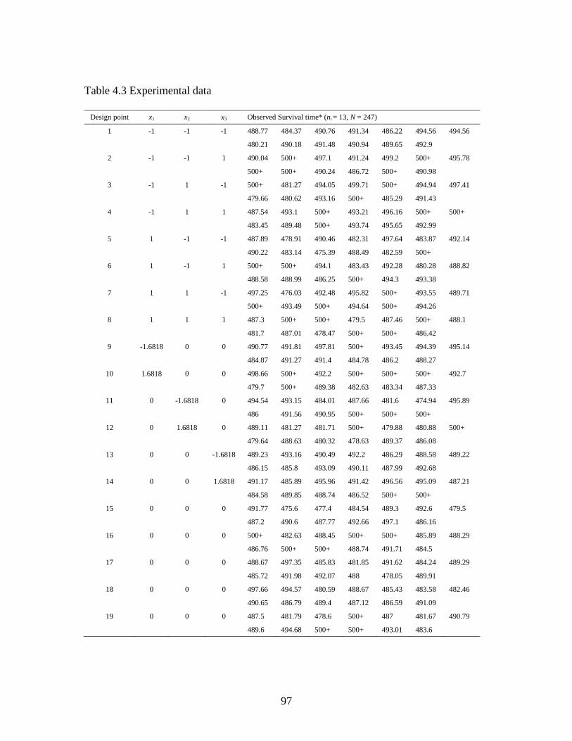
97
Table 4.3 Experimental data
Design point x1 x2 x3 Observed Survival time* (ni = 13, N = 247)
1 -1 -1 -1 488.77 484.37 490.76 491.34 486.22 494.56 494.56
480.21 490.18 491.48 490.94 489.65 492.9
2 -1 -1 1 490.04 500+ 497.1 491.24 499.2 500+ 495.78
500+ 500+ 490.24 486.72 500+ 490.98
3 -1 1 -1 500+ 481.27 494.05 499.71 500+ 494.94 497.41
479.66 480.62 493.16 500+ 485.29 491.43
4 -1 1 1 487.54 493.1 500+ 493.21 496.16 500+ 500+
483.45 489.48 500+ 493.74 495.65 492.99
5 1 -1 -1 487.89 478.91 490.46 482.31 497.64 483.87 492.14
490.22 483.14 475.39 488.49 482.59 500+
6 1 -1 1 500+ 500+ 494.1 483.43 492.28 480.28 488.82
488.58 488.99 486.25 500+ 494.3 493.38
7 1 1 -1 497.25 476.03 492.48 495.82 500+ 493.55 489.71
500+ 493.49 500+ 494.64 500+ 494.26
8 1 1 1 487.3 500+ 500+ 479.5 487.46 500+ 488.1
481.7 487.01 478.47 500+ 500+ 486.42
9 -1.6818 0 0 490.77 491.81 497.81 500+ 493.45 494.39 495.14
484.87 491.27 491.4 484.78 486.2 488.27
10 1.6818 0 0 498.66 500+ 492.2 500+ 500+ 500+ 492.7
479.7 500+ 489.38 482.63 483.34 487.33
11 0 -1.6818 0 494.54 493.15 484.01 487.66 481.6 474.94 495.89
486 491.56 490.95 500+ 500+ 500+
12 0 1.6818 0 489.11 481.27 481.71 500+ 479.88 480.88 500+
479.64 488.63 480.32 478.63 489.37 486.08
13 0 0 -1.6818 489.23 493.16 490.49 492.2 486.29 488.58 489.22
486.15 485.8 493.09 490.11 487.99 492.68
14 0 0 1.6818 491.17 485.89 495.96 491.42 496.56 495.09 487.21
484.58 489.85 488.74 486.52 500+ 500+
15 0 0 0 491.77 475.6 477.4 484.54 489.3 492.6 479.5
487.2 490.6 487.77 492.66 497.1 486.16
16 0 0 0 500+ 482.63 488.45 500+ 500+ 485.89 488.29
486.76 500+ 500+ 488.74 491.71 484.5
17 0 0 0 488.67 497.35 485.83 481.85 491.62 484.24 489.29
485.72 491.98 492.07 488 478.05 489.91
18 0 0 0 497.66 494.57 480.59 488.67 485.43 483.58 482.46
490.65 486.79 489.4 487.12 486.59 491.09
19 0 0 0 487.5 481.79 478.6 500+ 487 481.67 490.79
489.6 494.68 500+ 500+ 493.01 483.6

98
Table 4.4 The survival distribution of observations taken at the first and second design
points
The first design point (i=1)
where [x1, x2, x3] = [-1,-1,-1]
The second design point (i=2)
where [x1, x2, x3] = [-1,-1, +1]
j 1 jt
1 jn 1 jd
1( )jS t j 2 jt
2 jn 2 jd
2( )jS t
1 480.21 13 1 0.9231 1 486.72 13 1 0.9231
2 484.37 12 1 0.8462 2 490.04 12 1 0.8462
3 486.22 11 1 0.7692 3 490.24 11 1 0.7692
4 488.77 10 1 0.6923 4 490.98 10 1 0.6923
5 489.65 9 1 0.6154 5 491.24 9 1 0.6154
6 490.18 8 1 0.5385 6 495.78 8 1 0.5385
7 490.76 7 1 0.4615 7 497.1 7 1 0.4615
8 490.94 6 1 0.3846 8 499.2 6 1 0.3846
9 491.34 5 1 0.3077 9 500 5 0 0.3846
10 491.48 4 1 0.2308 10 500 5 0 0.3846
11 492.9 3 1 0.1538 11 500 5 0 0.3846
12 494.56 2 1 0.0769 12 500 5 0 0.3846
13 494.56 1 1 0.0000 13 500 5 0 0.3846
Figure 4.2 Survival curve of design points 1-5

99
Table 4.5 Median survival time, standard error of median survival time, and variance of
median survival time at each design point
Design point ith x1 x2 x3 M ( )Var M ( )SE M
1 -1 -1 -1 490.76 0.5974 0.7729
2 -1 -1 1 497.1 22.7452 4.7692
3 -1 1 -1 494.05 4.4226 2.1029
4 -1 1 1 493.74 2.3342 1.5278
5 1 -1 -1 487.89 10.2747 3.2054
6 1 -1 1 492.28 7.4644 2.7321
7 1 1 -1 494.64 1.8498 1.3601
8 1 1 1 487.46 0.4265 0.6531
9 -1.6818 0 0 491.4 0.3883 0.6231
10 1.6818 0 0 492.7 30.9143 5.5601
11 0 -1.6818 0 491.56 10.8195 3.2893
12 0 1.6818 0 481.71 9.7067 3.1155
13 0 0 -1.6818 489.23 0.8403 0.9167
14 0 0 1.6818 491.17 2.5783 1.6057
15 0 0 0 487.77 3.5393 1.8813
16 0 0 0 488.74 4.1987 2.0491
17 0 0 0 488.67 4.2975 2.0731
18 0 0 0 487.12 1.5531 1.2462
19 0 0 0 489.6 5.1563 2.2708
Step 3: Testing the PH assumption. The constant proportional hazards assumption
is tested using the scaled Schoenfeld residuals (Grambsch and Therneau, 1994) using the
stphtest command. The result shows that the PH assumption is invalid for the initial PH
model since p-value < 0.05.
Step 4: Adjusting the fitted model. The inactive variables are removed one at a
time, and the adjusted model is retested until the PH assumption is satisfied. After
removing the four input variables 2 2
1 2 3 1 2, , ,x x x x x as shown on the right-hand side of
Table 4.6, the fitted function of proportional hazards rate is finally obtained as

100
2
2 3 1
1 2 1 3 2 3
0.0996 0.2683 0.1067ˆ exp0.1837 0.0716 0.1813
x x xH
x x x x x x
x
Using the stphtest command the PH assumption is checked once again. The result shows
that the the PH assumption of this model is now satisfied with p-value = 0.3709. Figure
4.3 presents the scaled Schoenfeld plots where the horizontal trend lines are pproximately
constant. This confirms that the proportional hazards rate is approximately constant over
time.
Table 4.6 Statistics associated with the fitted proportional hazard model
Init
ial
fitt
ed P
H m
od
el
x Coefficient SE Z P-value 95% CI
1x -0.039 0.089 -0.45 0.656 -0.213 0.134
2x -0.102 0.090 -1.13 0.258 -0.279 0.072
3x -0.262 0.087 -3.03 0.002 -0.431 -0.092
2
1x -0.099 0.092 -1.08 0.282 -0.280 0.081
2
2x 0.028 0.092 0.30 0.762 -0.153 0.209
2
3x 0.052 0.088 0.58 0.560 -0.122 0.225
1 2x x -0.178 0.109 -1.63 0.103 -0.392 0.036
1 3x x 0.067 0.109 0.61 0.540 -0.147 0.282
2 3x x 0.179 0.110 1.63 0.103 -0.036 0.393
Test of the regression model : P-value = 0.0362; Test of the proportional hazards assumption : P-value = 0.0001
Ad
just
ed f
itte
d P
H m
od
el x Coefficient SE Z P-value 95% Confidence interval
2x -0.100 0.089 -1.12 0.262 -0.274 0.074
3x -0.268 0.088 -3.07 0.002 -0.440 -0.097
2
1x -0.107 0.090 -1.19 0.235 -0.283 0.070
1 2x x -0.184 0.110 -1.67 0.095 -0.399 0.032
1 3x x -0.072 0.110 0.65 0.516 -0.145 0.288
2 3x x 0.181 0.111 1.63 0.102 -0.036 0.399
Test of the regression model : P-value = 0.0082; Test of the proportional hazards assumption : P-value = 0.3595

101
Figure 4.3 The scaled Schoenfeld plots (the first row from left to right: x2, x3, 2
1x ; the
second row from left to right: x1x2, x1x3, x2x3)
4.4.3 Optimization results and findings
Using the fitted functions obtained in Sections 4.4.1 and 4.4.2, the optimization results
based on the twelve models proposed in Section 4.3, are compared. Suppose that the
minimum survival time allowed is 495, the maximum standard error of the median
survival time allowed is 5, and the maximum proportional hazards allowed is 0.75. That
is, ˆ ( ) 495,M x ˆ ( ) 5,SE M x and ˆ ( ) 0.75.H x Maple® (2016) programming codes for
the twelve nonlinear programming models were developed, and the optimization results
are summarized in Table 4.8, where italicized numbers represent the predicted values. As
expected, all the optimum operating conditions satisfy the requirement for the operability
region associated with the proposed type I-right censored central composite design. Also,
the addition of constraints decreases the survival time and failure rate and increases the
variability of the median survival time.
-4-2
02
4
sca
led S
cho
en
feld
- x
2
475 480 485 490 495 500Time
bandwidth = .8
Test of PH Assumption
-3-2
-10
12
sca
led S
cho
en
feld
- x
3
475 480 485 490 495 500Time
bandwidth = .8
Test of PH Assumption
-10
12
3
sca
led S
cho
en
feld
- x
1x1
475 480 485 490 495 500Time
bandwidth = .8
Test of PH Assumption-2
02
sca
led S
cho
en
feld
- x
1x2
475 480 485 490 495 500Time
bandwidth = .8
Test of PH Assumption
-4-2
02
sca
led S
cho
en
feld
- x
1x3
475 480 485 490 495 500Time
bandwidth = .8
Test of PH Assumption
-4-2
02
4
sca
led S
cho
en
feld
- x
2x3
475 480 485 490 495 500Time
bandwidth = .8
Test of PH Assumption
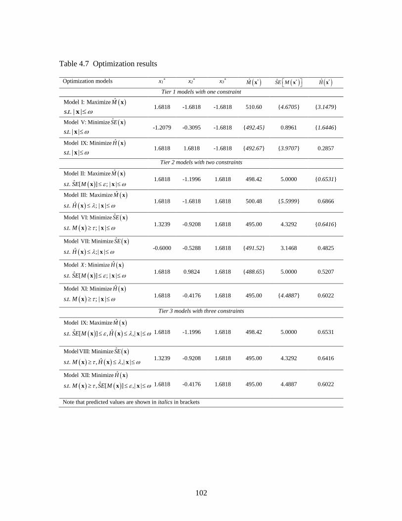
102
Table 4.7 Optimization results
Optimization models x1* x2
* x3* *M x *SE M
x *H x
Tier 1 models with one constraint
ˆModel I: Maximize M x
. . | |s t x 1.6818 -1.6818 -1.6818 510.60 {4.6705} {3.1479}
ˆModel V: Minimize SE x
. . | |s t x -1.2079 -0.3095 -1.6818 {492.45} 0.8961 {1.6446}
ˆModel IX: Minimize H x
. . | |s t x 1.6818 1.6818 -1.6818 {492.67} {3.9707} 0.2857
Tier 2 models with two constraints
ˆModel II: Maximize M x
ˆ. . [ ] ; | |s t SE M x x 1.6818 -1.1996 1.6818 498.42 5.0000 {0.6531}
ˆModel III: Maximize M x
ˆ. . ; | |s t H x x 1.6818 -1.6818 1.6818 500.48 {5.5999} 0.6866
ˆModel VI: Minimize SE x
. . ; | |s t M x x 1.3239 -0.9208 1.6818 495.00 4.3292 {0.6416}
ˆModel VII: Minimize SE x
ˆ. . ;| |s t H x x -0.6000 -0.5288 1.6818 {491.52} 3.1468 0.4825
ˆModel : MinimizeX H x
ˆ. . [ ] ; | |s t SE M x x 1.6818 0.9824 1.6818 {488.65} 5.0000 0.5207
ˆModel XI: Minimize H x
. . ; | |s t M x x 1.6818 -0.4176 1.6818 495.00 {4.4887} 0.6022
Tier 3 models with three constraints
ˆModel IX: Maximize M x
ˆ ˆ. . [ ] , ,| |s t SE M H x x x
1.6818 -1.1996 1.6818 498.42 5.0000 0.6531
ˆModel VIII: Minimize SE x
ˆ. . , ,| |s t M H x x x 1.3239 -0.9208 1.6818 495.00 4.3292 0.6416
ˆModel XII: Minimize H x
ˆ. . , [ ] ,| |s t M SE M x x x
1.6818 -0.4176 1.6818 495.00 4.4887 0.6022
Note that predicted values are shown in italics in brackets

103
Finally, the optimum operating conditions from Models I, III, and IX provide the longer
survival time in tiers 1, 2, and 3, respectively. Also, Models V, VII, and VIII provide a
smaller variability associated with the median survival time in each tier. Similarly, the
optimum operating conditions from Models IX, VII, and XII result in the lowest
proportional hazards rate in each tier.
4.5 Additional remarks on the parametric approach and recommendations
Under the type I-right censoring scheme, the distribution of censored data is very
likely to have a right-skewed shape, caused by the observations that are censored at the
censoring time. However, the actual distribution of the censored data is unknown and
may possibly follow a skewed distribution such as the exponential distribution, the
Weibull distribution, or the lognormal distribution. It is important to note that selecting
an inappropriate distribution may lead to inaccurate information that affects the ability to
make proper decisions on designing production processes and engineering systems,
resulting in product recalls and possibly the safety of end users. Therefore, the critical
part of analyzing the censored survival data is choosing the distribution that fits the data.
One of the methods used for fitting an appropriate distribution is the Anderson-Darling
(AD) goodness-of-fit test (see Anderson and Darling (1954)). In the case of censored
data, the AD test is computed based on the squared distance between a fitted distribution
line and the estimated cumulative probability based on the KM estimate of survival data.
As a result, selecting an appropriate distribution of the survival time using the AD test
statistic values can be done by seeking the smallest test statistic value among the set of
presumed distributions. To illustrate the parametric distribution fitting, the data used in

104
the numerical example is fitted to eleven parametric distributions. The AD goodness-of-
fit tests for the survival data are shown in Table 4.9 and Figure 4.5. For the particular data
set given in the numerical example, the most appropriate fitted distribution turns out to be
a 3-parameter log-logistic distribution.
As shown in Table 4.8 and Figure 4.4, we compare the mean and variability
obtained from the parametric survival analysis using the maximum likelihood estimator
(MLE) for the normal distribution, which is the default underlying distribution used in
RPD, with the median and standard error from the nonparametric survival analysis using
the KM estimator. The percentage of the difference between the MLE estimates xMLE and
the KM estimates xKM is given by ( ) 100%diff MLE KM MLE
i i i ix x x x i . Our results show
that the mean survival times using the MLE and the median survival times using the KM
estimator are very close to each other. However, the standard deviation of the survival
time using the MLE is slightly larger than the standard error of the median survival time
using the KM estimator. This result agrees well with the findings reported by Breslow
and Crowley (1974) that the survival distribution is known to converge weakly to a zero-
mean Gaussian process. Another explanation is that the standard deviation is calculated
using the entire set of observations, while the standard error is obtained by accounting
only the observations around the median survival time under a specific level of the type I
error, as shown in Equation (4.7). Finally, the AD test statistics in Table 4.9 indicate that
the data lacks a strong evidence for assuming the normal distribution. Hence, for this
particular right-censoring data, the use of the nonparametric KM estimator to obtain the
optimum operating conditions appears to be an effective method.

105
Figure 4.4 Comparison between the MLE estimator (left) and KM estimator (right)
Table 4.8 Comparing statistical estimators
Design
point
Number
of failure
time
Number of
censored
time
MLE KM Percent of difference
Mean Standard
deviation
Median Standard
error
Central
value
Variation
1 13 0 489.69 3.8994 490.76 2.1494 -0.0022 44.88
2 8 5 497.31 7.0543 497.1 3.4100 0.0004 51.66
3 10 3 493.38 9.3079 494.05 4.0622 -0.0014 56.36
4 9 4 495.52 6.8398 493.74 3.7184 0.0036 45.64
5 12 1 487.39 7.2921 487.89 4.0214 -0.0010 44.85
6 10 3 492.50 7.5987 492.28 3.9384 0.0004 48.17
7 9 4 496.06 8.3056 494.64 5.3856 0.0029 35.16
8 8 5 493.47 12.3592 487.46 5.5284 0.0122 55.27
9 12 1 491.70 4.8523 491.4 2.4870 0.0006 48.75
10 8 5 495.59 10.9868 492.7 5.2126 0.0058 52.56
11 10 3 491.97 9.2540 491.56 5.0049 0.0008 45.92
12 11 2 486.34 8.2484 481.71 3.8411 0.0095 53.43
13 13 0 489.62 2.5323 489.23 1.1024 0.0008 56.47
14 11 2 492.19 5.8776 491.17 2.7716 0.0021 52.84
15 13 0 487.09 6.1523 487.77 3.2204 -0.0014 47.66
16 8 5 494.53 10.1144 488.74 4.4602 0.0117 55.90
17 13 0 488.05 4.8001 488.67 2.8909 -0.0013 39.77
18 13 0 488.05 4.5691 487.12 2.5568 0.0019 44.04
19 10 3 490.94 8.9225 489.6 4.2739 0.0027 52.10

106
Table 4.9 Anderson-Darling test statistics for the experimental data
Distribution AD test statistics Correlation Coefficient
3-Parameter Loglogistic 287.380 0.998
3-Parameter Lognormal 287.415 0.998
3-Parameter Weibull 287.558 0.997
Lognormal 287.655 0.994
Normal 287.692 0.993
Loglogistic 288.120 0.983
Loglogistic 288.186 0.982
Weibull 292.046 0.965
Smallest Extreme Value 292.332 0.963
2-Parameter Exponential 299.491 *
Exponential 335.570 *
Figure 4.5 Probability plot of the experimental data
4.6 Process capability index for type I-right censored data
The process capability index (PCI) is a measure for evaluating and comparing
process performance in manufacturing and production processes. The vast selection of
PCI makes them becomes popular in practice, influencing researchers to continually

107
propose a customized PCI to better measure the capability in process environments.
Under censoring schemes, several PCIs are developed for assessing the performance of a
product based on its lifetime, known as the lifetime performance index. In particular,
Tong et al. (2002) proposed the lifetime index for exponentially distributed data. Along
the same lines, extensive studies were conducted by Wu et al. (2008) and Lee et al.
(2009), to incorporate the interferences of censoring into the exponential lifetime index.
On the other hand, lifetime indices based on other skewed distributions have been
proposed. Some noteworthy lifetime indices include the index for a Weibull distribution
(Ahmadi et al., 2013), a Weibull distribution with censoring (Lee, 2011; Hong et al.,
2012; Dey et al., 2016; and Wu and Lin, 2017), and a Rayleigh distribution with
censoring (Lee et al., 2011). Note that the PCI for assessing lifetime are modified based
on the same structure, LC LSL , where the and are estimated based on a
specific probability distribution. Although there remain challenging research gaps based
on parametric approaches with respect to censored data, this study focuses on the
development of PCI using nonparametric approach. It is because, as mentioned in Section
4.5, the distribution fitting of censored data may not provide sufficient evidence to
properly selecting the underlying distribution, which may lead to erroneous results of
subsequent calculations. In this regard, within the nonparametric scheme, the process
capability index for type I-right censored data and its confidence interval estimators are
developed in Section 4.6.1. Finally, the numerical example to illustrating the proposed
models is presented in Section 4.6.2.

108
4.6.1 Developments of PCI for type I-right censored data
Prior to the PCI development, the probability distribution of product’s lifetime
requires identification. Assume that observed survival time of a product is obtained under
type I-right censoring scheme and the probability distribution of observed survival time,
hereafter referred to as survival distribution, is estimated nonparametrically using KM
estimator (see Section 4.2.2). From this point forward, let T reduces to a 1 n matrix of
recorded survival time where jt T , 1,...,j n and 1j jt t j ; and ( )jS t denotes the
survival function of jt estimated from 1
( ) 1j
jS t d n
where jd ={0, for
censored observations; 1, for uncensored observations}, and jn is the number of units at
risk at time .jt As such, the survival distribution curve of the observed survival time is
then obtained by plotting time jt j versus its survival function ( )jS t j .
The definition of the PCI for type I-right censored data based on nonparamatric
survival distribution is given as the proportion of the width of actual conforming rate and
the width of the expected conforming rate. Since the survival distribution is constructed
nonparametrically, the statistical estimates are obtained using percentiles. Given LSL is
the lower specification limit (i.e., the minimum requirement of product’s lifetime), the
width of actual conforming rate is estimated from the survival probability correspoding to
LSL, i.e., the probability that products last longer than the LSL, which is defined as
( ) min ( )|j jS LSL S t t LSL . Similarly, the expected conforming rate is given as ,

109
where 0 1 . Therefore, the process capability index for type I-right censored data
based on nonparametric survival distribution is proposed as
max | ( ) 0
max | ( ) 0 min | ( )
j j
T
j j j j
t S t LSLC
t S t t S t
(4.10)
where max | ( ) 0j jt S t is the maximum recorded survival time of the entire
observations, min | ( )j jt S t is the survival time corresponding to the probability of
producing conforming units. Additionally, the numerator of TC , max | ( ) 0j jt S t LSL ,
denotes the width of specifications, and the denominator,
max | ( ) 0 min | ( )j j j jt S t t S t , represents the width of survival distribution, i.e.,
the variation of data, under the level of conforming rate . Therefore, the value of TC
consists of three types. Firstly, if min | ( )j jt S t LSL , we have TC = 1, implying that
the conforming rate of a process equals to the expected level . Secondly, if
min | ( )j jt S t LSL , then 1TC , which indicates that the conforming rate of a
process is lesser than . Thirdly, if min | ( )j jt S t LSL , we get 1TC , meaning
that the conforming rate of a process is higher than . Thus, the larger TC value is
preferred.
Furthermore, the nonconforming rate (ncp ), i.e., the probability that a unit fails to
meet a specification limit, is estimated from the survival function at the lower
specification limit, ( )S LSL ; see Figure 4.6 in Section 4.6.2. Note that the survival

110
function is a conditional probability function where 0 ( ) 1jS t , and is a decreased
probability function where max ( ) min | ( ) 1 1j j jS t S t S t . Thus, the nonconforming
rate is obtained from
min | ( ) 1 min | ( ) 1 ( )nc j j j j jp S t S t t LSL S t S t S LSL ; that is,
1 ( )ncp S LSL . Since ( ) min( ( ) | )i iS LSL S t t LSL . Therefore, the nonconforming
rate is expressed as
1 min( ( ) | )nc i ip S t t LSL (4.11)
The confidence interval approximation of TC can be manually calculated as follows. For
simplicity of the following derivations, let max | ( ) 0a j jt t S t and
min | ( ) .j jt t S t Thus, Equation (4.10) becomes aT
a
t LSLC
t t
. Since LSL is
given, the fluctuation of TC can be estimated from the confidence intervals of survival
functions associated with at and t . Suppose that the confidence intervals of
at and t
are ,L U
a at t and ,L Ut t , respectively. Based on the structure of TC , the lower
confidence bound of TC , L
TC , can be calculated from a proportion of the smallest
possible value of the numerator to the largest possible value of the denominator. On the
contrary, the upper confidence bound of TC , U
TC , is calculated from the ratio of the
largest value of numerator and the smallest value of denominator. As a result, the
confidence interval approximations of TC is estimated from

111
, ,L U
L U a aT T U L L U
a a
t LSL t LSLC C
t t t t
(4.12)
Consequently, the confidence intervals of jt under level of type I error are estimated
based on the corresponding confidence interval of its survival function. Given that
( ), ( )L U
j jS t S t are the lower bound and the upper bound of survival function of time jt .
Using Greenwood’s formula,
2
1
( ) ( )i
j j
dVar S t S t
n n d
(see Section 4.2.2
and Appendix A), the confidence intervals for ( )jS t is written as
2 2
( ), ( ) ( ) ( ) , ( ) ( )L U
j j j j j jS t S t S t z Var S t S t z Var S t (4.13)
where z is the 1th
percentile of the standard normal distribution, 0,1N .
Therefore, the confidence intervals of survival time jt is expressed as
, max | ( ) ( ) ,min | ( ) ( )L U U L
j j j j j j j jt t t S t S t t S t S t (4.14)
At this point, we have
2
2
max | ( ) ( ) ( ) ,
,
min | ( ) ( ) ( )
j j a aL U
a a
j j a a
t S t S t z Var S t
t t
t S t S t z Var S t
and
2
2
max | ( ) ( ) ( ) ,
,
min | ( ) ( ) ( )
j jL U
j j
t S t S t z Var S t
t t
t S t S t z Var S t
. Thus,
112
2
2 2
2
2 2
max | ( ) ( ) ( )
min | ( ) ( ) ( ) max | ( ) ( ) ( )
,
min | ( ) ( ) ( ),max | ( ) ( ) ( ) min | ( ) ( ) ( )
j j a a
j j a a j jL U
T T
j j a a
j j a a j j
t S t S t z Var S t LSL
t S t S t z Var S t t S t S t z Var S t
C C
t S t S t z Var S t LSL
t S t S t z Var S t t S t S t z Var S t
However, since max | ( ) 0a j jt t S t is the maximum observed survival time available
from observations, the upper bound of at U
at and its corresponding survival function
L
aS t is unobtainable. Therefore, 2
min | ( ) ( ) ( )U
a j j a a at t S t S t z Var S t t and
the previous equation of ,L U
T TC C becomes
2
2
2 2
max | ( ) ( ) ( ),
max | ( ) ( ) ( ),
max | ( ) ( ) ( ) min | ( ) ( ) ( )
j j a a
a j jL U
T T
a
j j a a j j
t S t S t z Var S t LSL
t t S t S t z Var S tC C
t LSL
t S t S t z Var S t t S t S t z Var S t
.
Finally, the confidence interval estimators of TC is rewritten in a simpler form as
, ,L
L U a aT T L L U
a a
t LSL t LSLC C
t t t t
(4.15)
4.6.2 Numerical example of the PCI for type I-right censored data
The calculation procedures of TC are illustrated using the data set of observed
failure time of 60 electrical appliances in a life test, as an adaptation of Lawless (2003).
Assume that the termination time of the test is 5,000 hours, the lower specification limit
is 500 hours, and 90% of the product is expected to last longer than 500 hours, i.e., the
conforming rate with respect to the lower specification limit be 0.90. Table 4.10 presents

113
the ranked failure time, survival functions, and the variance of the survival function. The
survival distribution based on KM estimator is shown in Figure 4.6. The TC is calculated
as follows. From Table 4.10, we get max | ( ) 0j jt S t = 4,584, min | ( ) 0.90j jt S t =
80. Since LSL = 500, using Equation (4.10) we have 0.9067TC . The nonconforming
rate of the electrical appliances is computed based on Equation (4.11), which is
1 min( ( ) | ) 1 0.7833 0.2167nc i ip S t t LSL . Furthermore, the confidence
intervals of TC are obtained from Equation (4.15). Given 0.05 , 0.025 1.96z ,
( ) 0.0833aS t , and [ ( )] 0.0357aVar S t ; we have ( ), ( )L U
a aS t S t 0.0134, 0.1533 .
As a result, 4,100L
at and 4,584U
a at t . Similarly, since
( ), ( ) 0.8241, 0.9759L US t S t , we get 34Lt and 381Ut . Finally, we obtain
, 0.7912, 1.0981L U
T TC C .
Figure 4.6 Survival distribution of the electrical appliances

114
Table 4.10 Observed failure time of the electrical appliances and its survival distribution
j tj nj dj S(tj) Var[S(tj)] j tj nj dj S(tj) Var[S(tj)]
1 14 60 1 0.9833 0.0165 31 1702 30 1 0.4833 0.0645
2 34 59 1 0.9667 0.0232 32 1893 29 1 0.4667 0.0644
3 59 58 1 0.9500 0.0281 33 1932 28 1 0.4500 0.0642
4 61 57 1 0.9333 0.0322 34 2001 27 1 0.4333 0.0640
5 69 56 1 0.9167 0.0357 35 2161 26 1 0.4167 0.0636
6 80 55 1 0.9000 0.0387 36 2292 25 1 0.4000 0.0632
7 123 54 1 0.8833 0.0414 37 2326 24 1 0.3833 0.0628
8 142 53 1 0.8667 0.0439 38 2337 23 1 0.3667 0.0622
9 165 52 1 0.8500 0.0461 39 2628 22 1 0.3500 0.0616
10 210 51 1 0.8333 0.0481 40 2785 21 1 0.3333 0.0609
11 381 50 1 0.8167 0.0500 41 2811 20 1 0.3167 0.0601
12 464 49 1 0.8000 0.0516 42 2886 19 1 0.3000 0.0592
13 479 48 1 0.7833 0.0532 43 2993 18 1 0.2833 0.0582
14 556 47 1 0.7667 0.0546 44 3122 17 1 0.2667 0.0571
15 574 46 1 0.7500 0.0559 45 3248 16 1 0.2500 0.0559
16 839 45 1 0.7333 0.0571 46 3715 15 1 0.2333 0.0546
17 917 44 1 0.7167 0.0582 47 3790 14 1 0.2167 0.0532
18 969 43 1 0.7000 0.0592 48 3857 13 1 0.2000 0.0516
19 991 42 1 0.6833 0.0601 49 3912 12 1 0.1833 0.0500
20 1064 41 1 0.6667 0.0609 50 4100 11 1 0.1667 0.0481
21 1088 40 1 0.6500 0.0616 51 4106 10 1 0.1500 0.0461
22 1091 39 1 0.6333 0.0622 52 4116 9 1 0.1333 0.0439
23 1174 38 1 0.6167 0.0628 53 4315 8 1 0.1167 0.0414
24 1270 37 1 0.6000 0.0632 54 4510 7 1 0.1000 0.0387
25 1275 36 1 0.5833 0.0636 55 4584 6 1 0.0833 0.0357
26 1355 35 1 0.5667 0.0640 56 5000+ 5 0 0.0833 0.0357
27 1397 34 1 0.5500 0.0642 57 5000+ 4 0 0.0833 0.0357
28 1477 33 1 0.5333 0.0644 58 5000+ 3 0 0.0833 0.0357
29 1578 32 1 0.5167 0.0645 59 5000+ 2 0 0.0833 0.0357
30 1649 31 1 0.5000 0.0645 60 5000+ 1 0 0.0833 0.0357
4.7 Concluding remarks
The proposed nonparametric RPD provides an effective approach for process
parameter optimization associated with time-oriented quality characteristics. Under a
censoring scheme, the traditional RPD method based on the normal distribution may not

115
be a suitable approach. Upon serving the purpose stated above, the guidelines for
estimating the response functions based on nonparametric approaches, including the KM
estimator, Greenwood’s formula, and the Cox PH model, are provided in this study.
Further, the applications of the proposed RPD method is not limited to the process
optimization problems under type I-right censoring with fixed starting time. The set of
methodologies developed in this chapter can also adapt to right censoring with random
starting time. As a result, the advantages of the nonparametric approaches employed in
RPD can enable applications of RPD in several potential research areas where time is the
quality characteristic of interest, such as reliability engineering, medical research, and
agriculture.
This chapter also develops optimization models that demonstrate the application
of nonparametric-based response functions. The case study results show that, although
the optimization models concerning all the three optimization criteria return similar
optimal values, the obtained optimum operating condition satisfy the minimum
requirement of survival time within the acceptable level of variation and proportional
hazards. Therefore, unlike the traditional RPD for time-oriented data, which only focus
on the average survival time and the variance of survival time, the proposed optimization
models with the consideration of the proportional hazard rate provide additional guidance
and confirmative information for making decisions under the quality improvement
scheme. In the particular numerical example used in this chapter, Models II and IX
provide the same expected median survival time, which implies that the upper bound of
the proportional hazards rate λ has been set relatively high. If the lower λ value were

116
specified, Model II would give longer expected median survival time. Also, it is observed
that the standard deviation of the survival time using the MLE is slightly larger than the
standard error of the median survival time using the KM estimator, mainly because the
survival distribution is known to converge weakly to a zero-mean Gaussian process.

117
CHAPTER 5
CONCLUSIONS AND FUTURE STUDIES
The original motivation for the dissertation is to develop a set of quality
engineering approaches for improving the accuracy of mathematical calculations when
solving engineering problems under the complications of incomplete data, i.e., the data
with partially known information. Failure to use appropriate statistical foundations for
analyzing the incomplete data could lead to aggregate errors of subsequent calculations,
resulting in the lack of accuracy when making decisions. Therefore, strengthening the
quality engineering approaches, such as the process capability index and the robust
parameter design, with consideration of the proper statistical foundations for incomplete
data bridges a noteworthy research gap. Despite a significant practical need, this research
gap has not been previously explored. Therefore, this chapter develops several quality
engineering approaches based on the appropriate statistical foundations for accurately
quantifying the incomplete data. These developments are summarized as follows.
Chapter 2: a set of the PCIs focused on the customer perception is developed for
accurately measuring the process capability of a product whose probability distribution
follows the truncated normal distribution. The truncated normal distribution parameters,
i.e., the mean and variance of truncated normal distribution, for two-sided truncated
distribution, left-sided truncated distribution, and right-sided truncated distribution are
derived in this chapter. Also, the data transformation-based PCI, which is the currently
recommended method for obtaining PCI concerning the truncated normal distribution, is

118
studied and is then compared to the proposed PCIs and the traditional PCIs. The
comparative study reveals that the proposed PCIs provide the largest index values and the
smallest defective rate, which seems more reasonable for evaluating the process
capability of the post-inspection products, which assume that non-conforming products
are removed prior to shipping to customers.
Chapter 3: two traditional target-based PCIs are modified to measure the process
capability with the consideration of the customer perception. Moreover, to complete the
development of the proposed PCIs regarding the truncated normal distribution, the
confidence interval approximations for CTN-p, CTN-pk, CTN-pm, and CTN-pmk are developed for
indicating the reliable of PCI values within a specific sample size. Furthermore, a
simulation technique is employed to study the features of the proposed PCIs compared to
its traditional counterparts across multiple scenarios. As a result, we found that the
proposed PCIs provide higher PCI values for a narrow range of truncation points, i.e.,
when a probability distribution is obviously truncated.
Chapter 4: a series of methods based on RPD is developed to obtain the optimum
operating conditions where experimental observations are type I-right censored. The
modification is applied to the three phases of RPD. Firstly, for the experimentation phase,
the central composite design is modified for dealing with censored data. The
nonparametric survival analysis methods, i.e., the KM estimator and Greenwood’s
formula, are utilized to estimating the median value and the variation of observations at
each design point. Secondly, in the response function development phase, the fitted
functions for the median survival time and the variance of the median survival time are

119
obtained based on multiple linear regression, and the fitted function for hazard rate is
estimated using the Cox PH model. Thirdly, the optimization models for obtaining the
optimum operating conditions based on the three fitted functions are proposed in the
optimization phase. From the numerical example, the optimization results indicate that,
under nonparametric assumptions, the proposed optimization models return the optimum
operating conditions that meet the requirements of the design, with guidance information
of the product’s reliability based on its survival time. Also, insights regarding the
parametric based survival analysis methods for RPD are provided. Furthermore, we
expand the application of the nonparametric statistical estimators for type I-right
censored data to redesign the process capability index for assessing the performance of a
product based on its observed survival times.
The future studies are summarized in Table 5.1. Although the collection of the
customer-perceived PCIs developed in this chapter could handle several cases in
practices, there are still opportunities for further enhancements. Since the proposed PCIs
are a univariate analysis, which are designed to measure the process capability based on a
single quality characteristics, a future study regarding how the truncated distribution
affects an intersected tolerance region in multivariate PCIs and the development of
multivariate PCIs concerning the effects of a truncated distribution would be another
interesting topic. Moreover, since the data involving the capability measurement in
services industries is generally a time-oriented data, the further extensions may
investigate the effects of censoring in a non-normal distribution, such as the exponential

120
distribution or the Weibull distributions. With extensions of the censoring-based PCI, the
service industries may benefit from future process capability analyses.
Moreover, under the RPD scheme, despite the fact that the type I-right censoring
is a preferred censoring mechanism for a critical reliability study and medical research, it
is considered as an expensive reliability experiment and may be unsuitable for some
situations, for instance, to study the failure of an electronic component that is designed to
last for years. A counterpart censoring mechanism such as the type I-right censoring
which may reduce the duration of an experiment, e.g., an experiment is terminate after
the third failure regardless of time, seems to be a considerable alternative. It is important
to note that since the data from type II-right censoring is partially observed, the survival
distribution of type II-right censoring is then estimated based on parametric approaches.
To strengthen the connection between the time-oriented quality characteristics and RPD,
it is of interest to develop RPD for time-oriented data based on type II-right censoring.
Furthermore, an adaptation of RPD method using another survival analysis approach such
as the accelerated failure time, which allows experimenters to speed up failure time by
testing a unit under an extreme environmental setting, is also an important future study.
The optimization phase in Chapter 4 could be extended as follows. Since the
optimization criteria have different units of measurement, which are also conflicted, the
optimization models are developed based on the single objective optimization. Under
those circumstances, the most important criterion is prioritized by being set as an
objective function while the other criteria are forced to be the optimization constraints.
Hence, to optimize the criteria as objective functions simultaneously, the multi-objective

121
optimization could be incorporated as a potential extension of this study. Ultimately, the
future developments of quality improvement methods concerning the effects of
incomplete data is not only a remarkable research opportunity for academia, but its
contributions could also provide more accurate information for improving the level of
quality in both manufacturing and services industries.
Table 5.1 Future studies
Chapters Limitations Future studies
Chapters 2 and 3 The proposed PCIs are derived by
setting the truncation points at the
specification limits. Therefore, these
PCIs are invalid if the specification
limits and the truncation points are
different.
Extensions of the proposed customer-perceived PCIs
(the truncation points are set at the specification limits)
- Sampling plan for the resubmitted lot
- Criterion for supplier selection
Manufacturing-based PCIs for the truncated normal
distribution (the specifications and the truncation points
are set differently)
- Process capability analysis for gap tolerance
- Process capability analysis for data with limitation of
devices
Chapter 4
Nonparametric method requires a
full set of observations, which may
be unobtainable in some situations.
Extensions of the proposed RPD for censored data
- RPD for type II-right censored data
- RPD for time-dependent variables
- Modifications of the optimization phase by
incorporating these following concepts
- Multi-objective optimization model
- Desirability function
- Multivariate optimization
Extensions of the proposed PCI for censored data
- Distribution-free PCIs for lifetime performance
assessment
- PCIs for duration data

122
APPENDICES

123
Appendix A
Derivation of Greenwood’s Formula
To start with, we simplify the product term of Equation (1) by taking the log of both sides
of the equation, as shown in Equation (A.1).
1
log ( ) log 1j
iij
i
dS t
n
. (A.1)
Thus, the variance of log ( )ijS t is given by
1
log ( ) log 1j
iij
i
dVar S t Var
n
(A.2)
Note that, for the further derivation, these following assumptions should hold. First,
assume that ijY is the number of units that survive through the interval 1,ij ijt t ,
ij ij ijY n d , which is independent and is binomially distributed, ,ij ij ijY B n p , where
ijn is a number of units at risk at time ijt and the ijp is the success rate of survival,
ij ij ij
ij
ij ij
n d Yp
n n
. Therefore, from Equation (A.2), log ( )ijVar S t can be estimated by
1 1
log ( ) log logj j
ij i i iVar S t Var p Var Y n
(A.3)
Second, from the first assumption, it yields that the random variable ijY is uncorrelated.
Therefore, the covariance terms are zero, so that 1
logj
i iVar Y n
is equal to
1
log .j
i iVar Y n
Thus, Equation (A.3) becomes
1
log ( ) logj
ij i iVar S t Var Y n
(A.4)

124
Third, for large N, the binomial random variable ,ij ij ijY B n p can be approximated as
, 1 .ij ij ij ij ij ijY N n p n p p Consequently, we obtain ˆijY ij ijn p and
2ˆ 1 .ijY ij ij ijn p p Thus, using the delta method based on the Taylor series expansions;
that is, if 2,X N and g(X ) is a functional form of X, then
2 2,g X N g g' , we obtain ( ) ( )E g X g and
2 2( )Var g X g . From 2ˆ ˆ, ,
ij ijij Y YY N using the delta method for estimating
function log( )ijY , we have
2
2Var log( ) logij ijij Y Y
dY
dx
(A.5)
From ( ) ( ) ( )ij ij ij ij ij ij ij ijE Y n E Y n n p n p and
2 2( ) ( ) ( (1 )) ( (1 ))ij ij ij ij ij ij ij ij ij ij ijVar Y n Var Y n n p p n p p n , log ij ijVar Y n is
calculated as
2
2
1 11log log
ij ij ij
ij ij ij ij ij ij
ij ij ij ij
p p pdVar Y n E Y n Var Y n
dx p n p n
. Since
ij ij
ij
ij
n dp
n
, we have
log
ij
ij ij
ij ij ij
dVar Y n
n n d
. Thus, Equation (A.4) becomes
1
log ( )j
iij
i i i
dVar S t
n n d
(A.6)
Similarly, based on the delta method, we have the variance of the exponential function of
ijY as 2
2Yij ij
ij
Y
Y
dVar e e
dx
. From log ( )
( ) ijS t
ijS t e and log ( )
( ) ijS t
ijVar S t Var e
,
we obtain
2
log ( )( ) log ( )
ijE S t
ij ijVar S t e Var S t (A.7)

125
From 1
log ( ) logj
ij i iE S t E Y n
,
1 1 1 1
1
log log log logj
i i ij ij ij ij i iE Y n E Y n E Y n E Y n
, and
log log log log 1ij
ij ij ij ij ij
ij
dE Y n E Y n p
n
, we have
1
log ( ) log 1 log ( )j
ij
ij ij
ij
dE S t S t
n
. Thus,
2
log ( )( ) log ( )ijS t
ij ijVar S t e Var S t . Finally, the estimated variance of the survival
function, also known as Greenwood’s formula (see Greenwood, 1926), is written as
2
1
( ) ( )j
iij ij
i i i
dVar S t S t
n n d
.
Although Greenwood’s formula is said to be a consistent estimate of the variance of the
survival function based on the KM estimator (Brookmeyer and Crowley, 1982) and has
been used widely among researchers, there are discussions regarding the assumptions of
Greenwood’s formula. Additionally, the nonparametric likelihood ratio method is
proposed in Thomas and Grunkemeier (1975) as an alternative confidence intervals
estimation for the nonparametric survival function without using the normal
approximation to the binomial. Li (1995) provides discussions regarding the performance
of Greenwood’s formula and the nonparametric likelihood ratio method. Moreover, the
modification of Greenwood’s formula based on the correlated random variables is studied
in Kang and Koehler (1997).

126
Appendix B
Derivation of the Variance of Survival Time
The delta method for estimating the variance of a density function is given as
2
( )d
Var g X g X Var Xdx
. Since ( )ijS t is a cumulative probability function of
,ijt we have
2
( ( ))( ( )) ( )
( )
dS t pVar S t p Var t p
dt p
(B.1)
where ( )t p is the time at (100p)th percentile of a distribution. Let ( ( )) ( ( ))f t p S' t p be
the estimated probability density function at survival time ( )t p . Using the mean value
theory to estimate the ( ( ))S' t p where ( ( ))S t p is a decreased function, we have
( ( ))( ( )) ( ( ))
( )
S t pf t p S' t p
t p
. Given that p is the confidence intervals of interest
where is the probability of type I error, we obtain( ( )) ( ( ))
( ( ))( ) ( )
S t p S t pf t p
t p t p
.
Thus, Equation (B.1) becomes 2
( ( )) ( ( )) ( )Var S t p f t p Var t p . Finally, the variance
of ( )t p is expressed as
2
( ( ))( )
( ( ))
Var S t pVar t p
f t p .

127
Appendix C
Minitab Output for Chapter 4
Response Surface Regression of ˆ ( )M x
Analysis of Variance
Source DF Adj SS Adj MS F-Value P-Value
Model 9 138.038 15.3375 1.79 0.199
Linear 3 25.486 8.4954 0.99 0.440
X1 1 2.156 2.1561 0.25 0.628
X2 1 15.835 15.8350 1.85 0.207
X3 1 7.495 7.4952 0.88 0.374
Square 3 60.831 20.2771 2.37 0.139
X1*X1 1 46.127 46.1270 5.38 0.045
X2*X2 1 0.079 0.0793 0.01 0.925
X3*X3 1 19.142 19.1418 2.23 0.169
2-Way Interaction 3 51.720 17.2400 2.01 0.183
X1*X2 1 41.496 41.4961 4.84 0.055
X1*X3 1 9.724 9.7241 1.14 0.314
X2*X3 1 0.500 0.5000 0.06 0.815
Error 9 77.093 8.5659
Lack-of-Fit 5 73.431 14.6862 16.04 0.009
Pure Error 4 3.662 0.9154
Total 18 215.131
Model Summary
S R-sq R-sq(adj) R-sq(pred)
2.92675 64.16% 28.33% 0.00%
Coded Coefficients
Term Effect Coef SE Coef T-Value P-Value VIF
Constant 488.28 1.31 373.49 0.000
X1 0.795 0.397 0.792 0.50 0.628 1.00
X2 -2.154 -1.077 0.792 -1.36 0.207 1.00
X3 -1.482 -0.741 0.792 -0.94 0.374 1.00
X1*X1 3.677 1.838 0.792 2.32 0.045 1.04
X2*X2 -0.152 -0.076 0.792 -0.10 0.925 1.04
X3*X3 2.368 1.184 0.792 1.49 0.169 1.04
X1*X2 -4.56 -2.28 1.03 -2.20 0.055 1.00
X1*X3 -2.21 -1.10 1.03 -1.07 0.314 1.00
X2*X3 0.50 0.25 1.03 0.24 0.815 1.00
Regression Equation in Uncoded Units
Median = 488.28 + 0.397 X1- 1.077 X2 - 0.741 X3 + 1.838 X1*X1 - 0.076 X2*X2
+ 1.184 X3*X3 - 2.28 X1*X2 - 1.10 X1*X3 + 0.25 X2*X3
Fits and Diagnostics for Unusual Observations
Obs Median Fit Resid Std Resid
9 481.71 486.26 -4.55 -2.48 R
12 493.74 489.86 3.88 2.30 R

128
Response Surface Regression for ˆ ( )SE M x versus A, B, X3
Analysis of Variance
Source DF Adj SS Adj MS F-Value P-Value
Model 9 15.6511 1.73902 1.65 0.234
Linear 3 8.1166 2.70553 2.56 0.120
X1 1 2.2640 2.26400 2.15 0.177
X2 1 0.7584 0.75840 0.72 0.419
X3 1 5.0942 5.09419 4.83 0.056
Square 3 7.1381 2.37936 2.25 0.151
X1*X1 1 0.9551 0.95505 0.90 0.366
X2*X2 1 2.9791 2.97915 2.82 0.127
X3*X3 1 2.3142 2.31418 2.19 0.173
2-Way Interaction 3 0.3965 0.13216 0.13 0.943
X1*X2 1 0.2375 0.23754 0.23 0.647
X1*X3 1 0.0918 0.09179 0.09 0.775
X2*X3 1 0.0672 0.06716 0.06 0.807
Error 9 9.4991 1.05545
Lack-of-Fit 5 6.6413 1.32827 1.86 0.284
Pure Error 4 2.8577 0.71444
Total 18 25.1502
Model Summary
S R-sq R-sq(adj) R-sq(pred)
1.02735 62.23% 24.46% 0.00%
Coded Coefficients
Term Effect Coef SE Coef T-Value P-Value VIF
Constant 3.456 0.459 7.53 0.000
X1 0.814 0.407 0.278 1.46 0.177 1.00
X2 0.471 0.236 0.278 0.85 0.419 1.00
X3 1.221 0.611 0.278 2.20 0.056 1.00
X1*X1 0.529 0.265 0.278 0.95 0.366 1.04
X2*X2 0.934 0.467 0.278 1.68 0.127 1.04
X3*X3 -0.823 -0.412 0.278 -1.48 0.173 1.04
X1*X2 -0.345 -0.172 0.363 -0.47 0.647 1.00
X1*X3 -0.214 -0.107 0.363 -0.29 0.775 1.00
X2*X3 0.183 0.092 0.363 0.25 0.807 1.00
Regression Equation in Uncoded Units
SE = 3.456 + 0.407X1 + 0.236X2 + 0.611 X3 + 0.265 X1*X1 + 0.467 X2*X2 - 0.412 X3*X3
- 0.172 X1*X2 - 0.107 X1*X3 + 0.092 X2*X3
Fits and Diagnostics for Unusual Observations
Obs SE Fit Resid Std Resid
9 3.841 5.174 -1.333 -2.07 R

129
Figure C.1 Residual Plots for (left) ˆ ( )M x (right) ˆ ( )SE M x
Figure C.2 Normality plot for error terms of ˆ ( )M x and ˆ ( )SE M x at 95% confidence
interval

130
Appendix D
Numerical Programming Code
Simulation code for Chapter 3 (Matlab®)
%Scenario1 LSL=-3, USL=3, target=0, mean=0, sigma=1, truncation
effect=Low, mean_location=Centered
clear all; clc;
filename = 'scenario1-n500.xlsx';
rep = 10000;N = 5000; n = 500; USL = 3; LSL = -3; target = (USL + LSL)/2; mu = 0; sigma = 1;
pop_table = zeros(rep,N); stat_pop = zeros(rep,10); PCIs_pop = zeros(rep,12);
samp_table = zeros(rep,N); stat_samp = zeros(rep,10); PCIs_samp = zeros(rep,12);
diff_PCIs = zeros(rep,8);
i=1; j=1;
while i <= rep ;
%generate population pop = mu + (((USL-LSL)/6)*randn(1,N));
mean = sum(pop)/N; sigma = std(pop);
%%PCIs calculation pdfLSL = normpdf(LSL,mean,sigma); cdfLSL = normcdf(LSL,mean,sigma);
pdfUSL = normpdf(USL,mean,sigma); cdfUSL = normcdf(USL,mean,sigma);
zLSL = (LSL-mean)/sigma ; zUSL = (USL-mean)/sigma ;
meanTN = mean + sigma*((pdfLSL-pdfUSL)/(cdfUSL-cdfLSL));
sigmaTN= (sqrt( sigma^2 * (1+((zLSL*pdfLSL - zUSL*pdfUSL)/(cdfUSL -
cdfLSL))- ((pdfLSL - pdfUSL)/( cdfUSL - cdfLSL))^2 )));

131
Cp =(USL-LSL)/(6*sigma); Ctnp = (USL-LSL)/(6*sigmaTN);
Cpl =(mean-LSL)/(3*sigma); Ctnpl = (meanTN-LSL)/(3*sigmaTN);
Cpu =(USL-mean)/(3*sigma); Ctnpu = (USL-meanTN)/(3*sigmaTN);
Cpk = min(Cpl, Cpu); Ctnpk = min(Ctnpl, Ctnpu);
Cpm=(USL-LSL)/(6*sqrt(sigma^2+(mean-target)^2)); Ctnm=(USL-LSL)/(6*sqrt(sigmaTN^2+(meanTN-target)^2));
Cpmk = Cpk / sqrt(1+((mean-target)/sigma)^2) ; Ctnpmk = Ctnpk / sqrt(1+((mean-target)/sigma)^2) ;
%storing values pop_table(i,:) = pop; stat_pop(i,:) = [mean; sigma; pdfLSL; cdfLSL; pdfUSL; cdfUSL; zLSL;
zUSL; meanTN; sigmaTN]; PCIs_pop(i,:) = [Cp; Ctnp; Cpl; Ctnpl; Cpu; Ctnpu; Cpk; Ctnpk; Cpm;
Ctnm; Cpmk; Ctnpmk]; %%end PCIs for pop
samp = datasample(pop,n); mean = sum(samp)/n; sigma = std(samp);
%%PCIs calculation pdfLSL = normpdf(LSL,mean,sigma); cdfLSL = normcdf(LSL,mean,sigma);
pdfUSL = normpdf(USL,mean,sigma); cdfUSL = normcdf(USL,mean,sigma);
zLSL = (LSL-mean)/sigma ; zUSL = (USL-mean)/sigma ;
meanTN = mean + sigma*((pdfLSL-pdfUSL)/(cdfUSL-cdfLSL));
sigmaTN= (sqrt( sigma^2 * (1+((zLSL*pdfLSL - zUSL*pdfUSL)/(cdfUSL -
cdfLSL))- ((pdfLSL - pdfUSL)/( cdfUSL - cdfLSL))^2 )));
Cp =(USL-LSL)/(6*sigma); Ctnp = (USL-LSL)/(6*sigmaTN);
Cpl =(mean-LSL)/(3*sigma); Ctnpl = (meanTN - LSL)/(3*sigmaTN);
132
Cpu =(USL-mean)/(3*sigma); Ctnpu = (USL-meanTN)/(3*sigmaTN);
Cpk = min(Cpl, Cpu); Ctnpk = min(Ctnpl, Ctnpu);
Cpm = (USL-LSL)/(6*sqrt(sigma^2+(mean-target)^2)); Ctnm = (USL-LSL)/(6*sqrt(sigmaTN^2+(meanTN-target)^2));
Cpmk = Cpk / sqrt(1+((mean-target)/sigma)^2) ; Ctnpmk = Ctnpk / sqrt(1+((mean-target)/sigma)^2) ;
%storing values samp_table(i,:) = pop; stat_samp(i,:) = [mean; sigma; pdfLSL; cdfLSL; pdfUSL; cdfUSL; zLSL;
zUSL; meanTN; sigmaTN]; PCIs_samp(i,:) = [Cp; Ctnp; Cpl; Ctnpl; Cpu; Ctnpu; Cpk; Ctnpk; Cpm;
Ctnm; Cpmk; Ctnpmk]; %%end PCIs for samples
%diff_PCIs(i,:) = PCIs_samp(i,:)- PCIs_pop(i,:);
i=i+1; end;
avg_pop = sum(PCIs_pop)/rep avg_samp = sum(PCIs_samp)/rep
%write to Excel file
tab_head_stat = {'mean', 'sigma', 'pdf LSL', 'cdf LSL', 'pdf USL', 'cdf
USL', 'meanTN', 'sigmaTN'}; tab_head_PCIs = {'C_p', 'CTN-p','Cpl', 'Ctnpl', 'Cpu', 'Ctnpu', 'Cpk',
'Ctnpk', 'Cpm', 'Ctnm', 'Cpmk', 'Ctnmk'}; tab_head_blank = {' ', ' ',' ', ' ', ' ', ' ', ' ', ' ', ' ', ' ', ' ',
' '};
xlswrite(filename, tab_head_stat, 'stat_pop'); xlswrite(filename, stat_pop, 'stat_pop', 'A2');
xlswrite(filename, tab_head_PCIs, 'PCIs_pop', 'A1'); xlswrite(filename, PCIs_pop, 'PCIs_pop', 'A2'); xlswrite(filename, tab_head_PCIs, 'PCIs_samp', 'R1'); xlswrite(filename, avg_pop, 'PCIs_pop', 'R2');
xlswrite(filename, tab_head_stat, 'stat_samp', 'A1'); xlswrite(filename, stat_samp, 'stat_samp', 'A2');
xlswrite(filename, tab_head_PCIs, 'PCIs_samp', 'A1'); xlswrite(filename, PCIs_samp, 'PCIs_samp', 'A2');

133
xlswrite(filename, tab_head_PCIs, 'PCIs_samp', 'R1'); xlswrite(filename, avg_samp, 'PCIs_samp', 'R2');
x0=10;y0=10;width=600;height=300; set(gcf,'units','points','position',[x0,y0,width,height])
%drawing Boxplot
boxplot(PCIs_samp, 'Labels', tab_head_blank); ylim([0 2]) set(gca,'XTick',[]); [hx,hy] = format_ticks(gca,{'\itC_p', '\itC_{T-p}','\itC_{pl}',
'\itC_{T-pl}', '\itC_{pu}', '\itC_{T-pu}', '\itC_{pk}', '\itC_{T-pk}',
'\itC_{pm}', '\itC_{T-pm}', '\itC_{pmk}', '\itC_{T-pmk}'},... [],[1:1:12]);
Optimization code for numerical example in Chapter 4 (Maple®)
>
>

134

135

136
REFERENCES
Anderson, T. W., & Darling, D. A. (1954). A test of goodness of fit. Journal of the
American Statistical Association, 49(268), 765-769.
Anis, M. Z. (2008). Basic process capability indices: An expository review.
International Statistical Review, 76(3), 347 - 367.
Asokan, M. V., & Unnithan, V. K. G. (1999). Estimation of vendor's process capability
from the lots screened to meet specifications. Quality Engineering, 11(4), 537-540.
Awad, M. I., & Kovach, J. V. (2011). Multiresponse optimization using multivariate
process capability index. Quality and Reliability Engineering International, 27, 465–
477.
Bao, L., Huang, Q., & Wang, K. (2016). Robust parameter design for profile quality
control. Quality and Reliability Engineering International, 32(3), 1059–1070.
Baş, D., & Boyacı, İ. H. (2007). Modeling and optimization I: Usability of response
surface methodology. Journal of Food Engineering, 78(3), 836-845.
Bissell, A. F. (1990). How reliable is your capability index? Applied Statistics, 39, 331–
340.
Bothe, D. R. (1992). A capability study for an entire product. Paper presented at
the ASQC Quality Congress Transactions, 46, 172-178.
Box G. E., & Cox D. R. (1964). An analysis of transformations. Journal of the Royal
Statistical Society. Series B (Methodological), 211-252.
Box, J., & Wilson, W. (1951). Central composites design. Journal of the Royal Statistics
society, 13(1), 1-35.
Boyles, R.A. (1991). The Taguchi capability index. Journal of Quality Technology,
23(1), 17–26.
Breslow, N., & Crowley, J. (1974). A large sample study of the life table and product
limit estimates under random censorship. The Annals of Statistics, 2(3), 437-453.
Brito, T. G., Paiva, A. P., Ferreira, J. R., Gomes, J. H. F., & Balestrassi, P. P. (2014). A
normal boundary intersection approach to multi-response robust optimization of the
surface roughness in end milling process with combined arrays. Precision
Engineering, 38(3), 628–638.

137
Brito, T. G., Paiva, A. P., T. I. Paula, Dalosto, D. N., Ferreira, J. R., & Balestrassi, P. P.
(2016). Optimization of AISI 1045 end milling using robust parameter design. The
International Journal of Advanced Manufacturing Technology, 84(5-8), 1185–1199.
Carter, W. H., Stablein, D. M., & Wampler, G. L. (1979). An improved method for
analyzing survival data from combination chemotherapy experiments. Cancer
Research, 39(9), 3446-3453.
Cha, J., Cho B. R., & Sharp J. L. (2013). Rethinking the truncated normal distribution.
International Journal of Experimental Design and Process Optimisation, 3(4), 327-
363.
Cha, J., & Cho, B. R. (2015). Classical statistical inference extended to truncated
populations for continuous process improvement: test statistics, P-values, and
confidence intervals. Quality and Reliability Engineering International, 31(8), 1807-
1824.
Chan, L., Cheng, S., & Spiring, F. (1991). A multivariate measure of process capability.
International Journal of Modelling and Simulation, 11(1), 1-6.
Chan, L. K., Cheng, S. W., & Spiring, F. A. (1988). A new measure of process capability
Cpm. Journal of Quality Technology, 20(3), 162-175.
Chang, Y. S., Choi, I. S., & Bai, D.S. (2002). Process capability indices for skewed
populations. Quality and Reliability Engineering International. 18(5), 383-393.
Chen, H. A. (1994). Multivariate process capability index over a rectangular solid
tolerance zone. Statistica Sinica, 4(2), 749-758.
Chen, K. S., & Pearn, W. L. (1997). Capability measures for processes with multiple
characteristics. Quality and Reliability Engineering International, 13, 355–360.
Chen, S. M., & Hsu, N. F. (1995). The asymptotic distribution of the process capability
index Cpmk. Communications in Statistics: Theory and Methods, 24(5), 1279-1291.
Cho, B. R., & Park, C. (2005). Robust design modeling and optimization with unbalanced
data. Computers & industrial engineering, 48(2), 173-180.
Cho, B. R., Choi, Y., & Shin, S. (2010). Development of censored data-based robust
design for pharmaceutical quality by design. The International Journal of Advanced
Manufacturing Technology, 49(9-12), 839-851.
Cho, B. R., Kim, Y. J., Kimbler, D. L., & Phillips, M. D. (2000). An integrated joint
optimization procedure for robust and tolerance design. International Journal of
Production Research, 38(10), 2309–2325.

138
Cho, B. R., & Leonard, M. S. (1997). Identification and Extensions of Quasiconvex
Quality Loss Functions. International Journal of Reliability, Quality and Safety
Engineering, 4(2), 191-204.
Choi, I. S., & Bai, D. S. (1996). Process capability indices for skewed distributions,
Proceedings of 20th International Conference on Computer and Industrial
Engineering. Kyongju, Korea, 1211–1214.
Chou, Y., Polansky, A. M., & Mason, R. L. (1998). Transforming non-normal data to
normality in statistical process control. Journal of Quality Technology, 30(2), 133-
141.
Chou, Y. M., Owen, D. B., & Borrego, A. S. A. (1990). Lower confidence limits on
process capability indices. Journal of Quality Technology, 22(3), 223–229.
Clements, J. A. (1989). Process capability calculations for non-normal distributions.
Quality Progress, 22, 95-100.
Cohen, A. C. (1991). Truncated and censored Samples. New York: Marcel Dekker.
Copeland, K., & Nelson, P. (1996). Dual response optimization via direct function
minimization. Journal of Quality Technology, 28, 331–336.
Cox, D. R. (1975). Partial likelihood. Biometrika, 269-276.
Cox, D. R., & Oakes, D. (1984). Analysis of survival data. London: Chapman and Hall.
Das, R. N. (2009). Response surface methodology in improving mean life time. In Prob-
Stat Forum, 2, 8-20.
Del Castillo, E., & Montgomery, D. C. (1993). A nonlinear programming solution to the
dual response problem. Journal of Quality Technology, 25(3), 199–204.
English, J. R., & Taylor, G. D. (1993). Process capability analysis – a robustness study.
International Journal of Production Research, 31, 1621–1635.
Eslamipoor, R., & Hosseini-nasab, H. (2016). A modified process capability index using
loss function concept. Quality and Reliability Engineering International, 32(2), 435-
442.
Fang, J., Gao, Y., Sun, G., Xu, C., & Li, Q. (2015). Multi-objective robust design
optimization of fatigue life for a truck cab. Reliability Engineering & System Safety,
135, 1–8.

139
Feigenbaum, A. V. (1951). Quality control: Principles, practice and administration: An
industrial management tool for improving product quality and design and for
reducing operating costs and losses. New York: McGraw Hill.
Goethals, P., & Cho, B. R. (2012). Designing the optimal process mean vector for mixed
multiple quality characteristics. IIE Transactions, 44, 1002-1021.
Goethals, P. L, & Cho, B. R. (2011). The development of a target‐focused process
capability index with multiple characteristics. Quality and Reliability Engineering
International, 27(3), 297-311.
Grambsch, P. M., & Therneau, T. M. (1994). Proportional hazards tests and diagnostics
based on weighted residuals. Biometrika, 81, 515–526.
Greenwood, M. (1926). The natural duration of cancer. His Majesty’s Stationery Office,
Reports on Public Health and Medical Subjects, No. 33. London, England
He, Z., Zhu, P. F., & Park, S. H. (2012). A robust desirability function method for multi-
response surface optimization considering model uncertainty. European Journal of
Operational Research, 221(1), 241–247.
Hong, S. H., & Cho, B. R. (2007). Joint optimization of process target mean and
tolerance limits with measurement errors under multi-decision
alternatives. European Journal of Operational Research, 183(1), 327-335.
Hosseinifard, S. Z., Abbasi, B., Ahmad, S., & Abdollahian, M. (2009). A transformation
technique to estimate the process capability index for non-normal processes. The
International Journal of Advanced Manufacturing Technology, 40(5-6), 512-517.
Hsieh, K.L., & Tong, L.I. (2006). Incorporating process capability index and quality loss
function into analyzing the process capability for qualitative data. The International
Journal of Advanced Manufacturing Technology, 27(11), 1217-1222.
Hu, Z., Du, X., Kolekar, N. S., & Banerjee, A. (2014). Robust design with imprecise
random variables and its application in hydrokinetic turbine optimization.
Engineering Optimization, 46(3), 393–419.
Hubele, N., Shahriari, H., & Cheng, C. (1991). A bivariate process capability
vector. Statistical Process Control in Manufacturing (Edited by Keats, J. B. &
Montgomery, D. C.). New York: Marcel Dekker.
Jeang, A., & Chung, C. P. (2009). Process capability analysis based on minimum
production cost and quality loss. International Journal of Advanced Manufacturing
Technology, 43(7), 710–719.

140
Johnson, N. L. (1949). Systems of frequency curves generated by methods of translation.
Biometrika, 149-176.
Johnson, N. L., Kotz, S., & Pearn, W. (1992). Flexible process capability
indices. Department of Statistics, University of North Carolina at Chapel Hill.
Johnson, N. L., & Kotz, S. (1970). Continuous univariate distributions, vol. 1, New
York: John Wiley and sons.
Juran, J. M. (1951). Quality Control Handbook, 1st ed. New York: McGraw Hill.
Juran, J. M. (1962). Quality Control Handbook, 2nd ed. New York: McGraw Hill.
Juran, J. M., & Gryna F.M. (1980). Quality Planning and Analysis, 2nd ed. New York:
McGraw Hill.
Kalbfleisch, J. D., & Prentice, R. L. (2011). The statistical analysis of failure time
data (Vol. 360). New York: John Wiley and sons.
Kane, V. E. (1986). Process capability indices. Journal of Quality Technology, 18(1), 41-
52.
Kang, S. S., & Koehler, K. J. (1997). Modification of the Greenwood formula for
correlated response times. Biometrics, 885-899.
Kaplan, E. L., & Meier, P. (1958). Nonparametric estimation from incomplete
observations. Journal of the American Statistical Association, 53(282), 457-481.
Khamkanya, A., Cho, B. R., & Goethals, P. L. (2016). Integrating customer perception
into process capability measures. Quality and Reliability Engineering International,
32(4), 1331-1345.
Khasawneh, M. T., Bowling, S. R., Kaewkuekool, S., & Cho, B.R. (2005). Tables of a
truncated standard normal distribution: A doubly truncated case. Quality
Engineering, 17(2), 227-241.
Khasawneh, M. T., Bowling, S. R., Kaewkuekool, S., & Cho, B. R. (2004). Tables of a
truncated standard normal distribution: A singly truncated case. Quality
Engineering, 17(1), 33-50.
Khuri, A. I., & Mukhopadhyay, S. (2010). Response surface methodology. Wiley
Interdisciplinary Reviews: Computational Statistics, 2(2), 128-149.
Kim, Y. J., & Cho, B. R. (2002). Development of priority-based robust design. Quality
Engineering, 14(3), 355–363.
141
Klein, J. P., & Moeschberger, M. L. (2005). Survival analysis: techniques for censored
and truncated data. New York: Springer Science & Business Media.
Kleinbaum, D. G., & Klein, M. (2006). Survival analysis: a self-learning text. New York:
Springer Science & Business Media.
Kotz, S., Johnson, N. L., Hubele, N. F., Spiring, F., Cheng, S., Yeung, A., & Lu, M.
(2002). Process capability indices: A review, 1992-2000. Discussions. Journal of
Quality Technology, 34(1), 2-53.
Kotz, S., & Lovelace, C. R. (1998). Process capability indices in theory and practice.
London: Hodder Education Publishers.
Kotz, S., & Johnson, N. L. (1993). Process capability indices, New York: Chapman and
Hall.
Kovach, J., & Cho, B. R. (2009). A D-optimal design approach for constrained
multiresponse robust design with prioritized mean and variance considerations.
Computers & Industrial Engineering, 57, 237-245.
Krenek, R., Cha, J., & Cho, B. R. (2016). Development of the convolutions of truncated
normal random variables with three different quality characteristics in engineering
applications. Computers & Industrial Engineering, 94, 125-137.
Kuhn, A. M., Carter, W. H., & Myers, R. H. (2000). Incorporating noise factors into
experiments with censored data. Technometrics, 42(4), 376-383.
Kushler, R., & Hurley, P. (1992). Confidence bounds for capability indices. Journal of
Quality Technology, 24(4), 188–195.
Kwak, J. S. (2005). Application of Taguchi and response surface methodologies for
geometric error in surface grinding process. International Journal of Machine Tools
and Manufacture, 45(3), 327-334.
Lawless, J. F. (2011). Statistical models and methods for lifetime data (Vol. 362). New
York: John Wiley and sons.
Lee, K. K., Park, C. K., & Han, S. H. (2010). Robust design of railway vehicle
suspension using a process capability index. Journal of Mechanical Science and
Technology, 24, 215–218.
Li, G. (1995). On nonparametric likelihood ratio estimation of survival probabilities for
censored data. Statistics & Probability Letters, 25(2), 95-104.

142
Li, Z., Cho, B. R., & Melloy, B. (2012a). A research and development effort in
developing the optimal formulations for new tablet drugs using design of
experiments: part 1 (dissolution comparisons), International Journal of
Experimental Design and Process Optimisation, 3(1), 43-67.
Li, Z., Cho, B. R., & Melloy, B. (2012b). A research and development effort in
developing the optimal formulations for new tablet drugs using design of
experiments: part 2 (bioequivalence studies), International Journal of Experimental
Design and Process Optimisation, 3(1), 68-90.
Li, Z., Cho, B. R., & Melloy, B. (2013). Quality by design studies on multi-response
pharmaceutical formulation modeling and optimization. Journal of Pharmaceutical
Innovation, 8, 28-44.
Lin, D. K. J., & Tu, W. (1995). Dual response surface optimization. Journal of Quality
Technology, 27(1), 34–39.
Lovelace C.R., & Swain J.J. (2009). Process capability analysis methodologies for zero-
bound, non-normal process data. Quality Engineering, 21(2), 190-202.
Maple Software (Version 2015), Maplesoft, Waterloo, Canada, 2016.
Mead, R., & Pike, D. J. (1975). A biometrics invited paper. A review of response surface
methodology from a biometric viewpoint. Biometrics, 31(4), 803-851.
Minitab Software (Version 17), Minitab, USA, 2016.
Montgomery, D. C. (2012). Introduction to statistical quality control, 7th ed. New York:
John Wiley and Sons.
Montgomery, D. C. (2013). Design and analysis of experiments, 8th ed. New York: John
Wiley and Sons.
Myers, R. H., Montgomery, D. C., & Anderson-Cook, C. M. (2016). Response surface
methodology: process and product optimization using designed experiments. New
York: John Wiley and Sons.
Nagata, Y., & Nagahata, H. (1994). Approximation formulas for the lower confidence
limits of process capability indices. Okayama Economic Review, 25(4), 301-314.
Nair, V. N., Abraham, B., MacKay, J., Box, G., Kacker, R. N., Lorenzen, T. J., &
Phadke, M. S. (1992). Taguchi's parameter design: a panel discussion.
Technometrics, 34(2), 127-161.

143
Ouyang, L., Ma, Y., Byun, J. H., Wang, J., & Tu, Y. (2016). An interval approach to
robust design with parameter uncertainty. International Journal of Production
Research, 54(11), 3201–3215.
Ozdemir, A., & Cho, B. R. (2016). A nonlinear integer programming approach to solving
the robust parameter design optimization problem. Quality and Reliability
Engineering International, 32(8), 2859–2870.
Ozdemir, A., & Cho, B. R. (2017). Response surface-based robust parameter design
optimization with both qualitative and quantitative variables. Engineering
Optimization, 1-17.
Park, C., & Cho, B. R. (2003). Development of robust design under contaminated and
non-normal data. Quality Engineering, 15(3), 463-469.
Park, G. J., Lee, T. H., Lee, K. H., & Hwang, K. H. (2006). Robust design: an
overview. AIAA journal, 44(1), 181-191.
Patnaik, P. B. (1949). The non-central χ2 and F-distributions and their approximations.
Biometrika, 36, 202–232.
Pearn, W. L, Hung, H., Peng, N., & Huang, C. (2007). Testing process precision for
truncated normal distributions. Microelectronics Reliability, 47(12), 2275-2281.
Pearn, W. L., & Kotz, S. (2006). Encyclopedia and handbook of process capability
indices. Singapore: World Scientific.
Pearn, W. L., & Lin, P. C. (2004). Testing process performance based on capability index
Cpk with critical values. Computers & Industrial Engineering, 47(4), 351-369.
Pearn, W. L., Kotz, S., & Johnson N. L. (1992). Distributional and inferential properties
of process control indices. Journal of Quality Technology, 24, 216–231.
Plante, R. D. (2001). Process capability: a criterion for optimizing multiple response
product and process design. IIE Transactions, 33(6), 497-509.
Polansky, A. M., Chou, Y. M., & Mason, R. L. (1998). Estimating process capability
indices for a truncated distribution. Quality Engineering, 11(2), 257-265.
Rivera, L. A. R., Hubele, N. F., & Lawrence, F. D. (1995). Cpk index estimation using
data transformation. Computer and Industrial Engineering, 29, 55–58.
Robinson, T. J., Borror, C. M., & Myers, R. H. (2004). Robust parameter design: a
review. Quality and Reliability Engineering International, 20(1), 81-101.

144
Shaibu, A. B., & Cho, B. R. (2009). Another view of dual response surface modeling and
optimization in robust parameter design. The International Journal of Advanced
Manufacturing Technology, 41(7-8), 631–641.
Shaibu, A. B., Cho, B. R., & Kovach, J. (2009). Development of a censored robust design
model for time‐oriented quality characteristics. Quality and Reliability Engineering
International, 25(2), 181-197.
Shin, S., & Cho, B. R. (2009). Studies on a bi-objective robust design optimization
problem. IIE Transactions, 41(11), 957-968.
Shin, S., & Cho, B. R. (2005). Bias-specified robust design optimization and its analytical
solutions. Computers & Industrial Engineering, 48(1), 129–140.
Solana, R. P., Chinchilli, V. M., Carter Jr, W. H., Wilson, J. D., & Carchman, R. A.
(1987). The evaluation of biological interactions using response surface
methodology. Cell Biology and Toxicology, 3(3), 263-277.
Spiring, F., Leung, B., Cheng, S., & Yeung, A. (2003). A bibliography of process
capability papers. Quality and Reliability Engineering International, 19(5), 445-460.
Stata Software (Version 14.1), StataCorp, College Station, TX, USA, 2016.
Stuart, A., & Ord, J. K. (1987). Kendall’s advanced theory of statistics, 5th ed. London:
Griffin.
Sweet, A. L., & Tu J. F. (2006). Evaluating tolerances and process capability when using
truncated probability density functions. International Journal of Production
Research, 44(17), 3493-3508.
Taguchi, G. (1986). Introduction to quality engineering. New York: UNIPUB.
Tang, L. C., & Than, S. E. (1999). Computing process capability indices for non-normal
data: a review and comparative study. Quality and Reliability Engineering
International, 15, 339–353.
Tao, L., & Xinzhang, J. (2012). An empirical formula for yield estimation from singly
truncated performance data of qualified semiconductor devices. Journal of
Semiconductors, 33(12), 1 – 7.
Thomas, D. R., & Grunkemeier, G. L. (1975). Confidence interval estimation of survival
probabilities for censored data. Journal of the American Statistical
Association, 70(352), 865-871.
Vännman, K. (1995). A unified approach to capability indices. Statistica Seneca, 5, 805-
820.

145
Vännman, K., & Kotz, S. (1995). A superstructure of capability indices: Distributional
properties and implications. Scandinavian Journal of Statistics, 477-491.
Vining, G. G., & Myers, R. H. (1990). Combining Taguchi and response surface
philosophies: A dual response approach. Journal of Quality Technology, 22(1), 38–
45.
Wang, F., & Chen, J. C. (1998). Capability index using principal components
analysis. Quality Engineering, 11(1), 21-27.
Wang, H., Yang, J., & Hao, S. (2016). Two inverse normalizing transformation methods
for the process capability analysis of non-normal process data. Computers &
Industrial Engineering, 102, 88-98.
Wilson, E. B., & Hilferty, M. M. (1931). The distribution of chi-square. Proceedings of
the National Academy of Sciences, 17(12), 684-688.
Wright, P. A. (1995). A process capability index sensitive to skewness. Journal of
Statistical Computation and Simulation, 52(3), 195-203.
Wu, H., & Swain, J. J. (2001). A monte carlo comparison of capability indices when
processes are non‐normally distributed. Quality and Reliability Engineering
International, 17(3), 219-231.
Wu, C. W., Shu, M. H., Nugroho, A. A., & Kurniati, N. (2015). A flexible process-
capability-qualified resubmission-allowed acceptance sampling scheme. Computers
& Industrial Engineering, 80, 62-71.
Yum, B., & Kim, K. (2011). A bibliography of the literature on process capability
indices: 2000–2009. Quality and Reliability Engineering International, 27(3), 251-
268.
Zhang, N. F., Stenback, G. A., & Wardrop, D. M. (1990). Interval estimation of process
capability index Cpk. Communications in Statistics-Theory and Methods, 19(12),
4455-4470.
Zimmer, L. S., Hubele, N. F., & Zimmer, W. J. (2001). Confidence intervals and sample
size determination for Cpm. Quality and Reliability Engineering International, 17(1),
51-68.