Embed Size (px)
Citation preview
Dissipative Particle Dynamics: Foundation, Evolution and Applications
George Em Karniadakis Division of Applied Mathematics, Brown University
& Department of Mechanical Engineering, MIT & Pacific Northwest National Laboratory, CM4
The CRUNCH group: www.cfm.brown.edu/crunch
Lecture 2: Theoretical foundation and parameterization
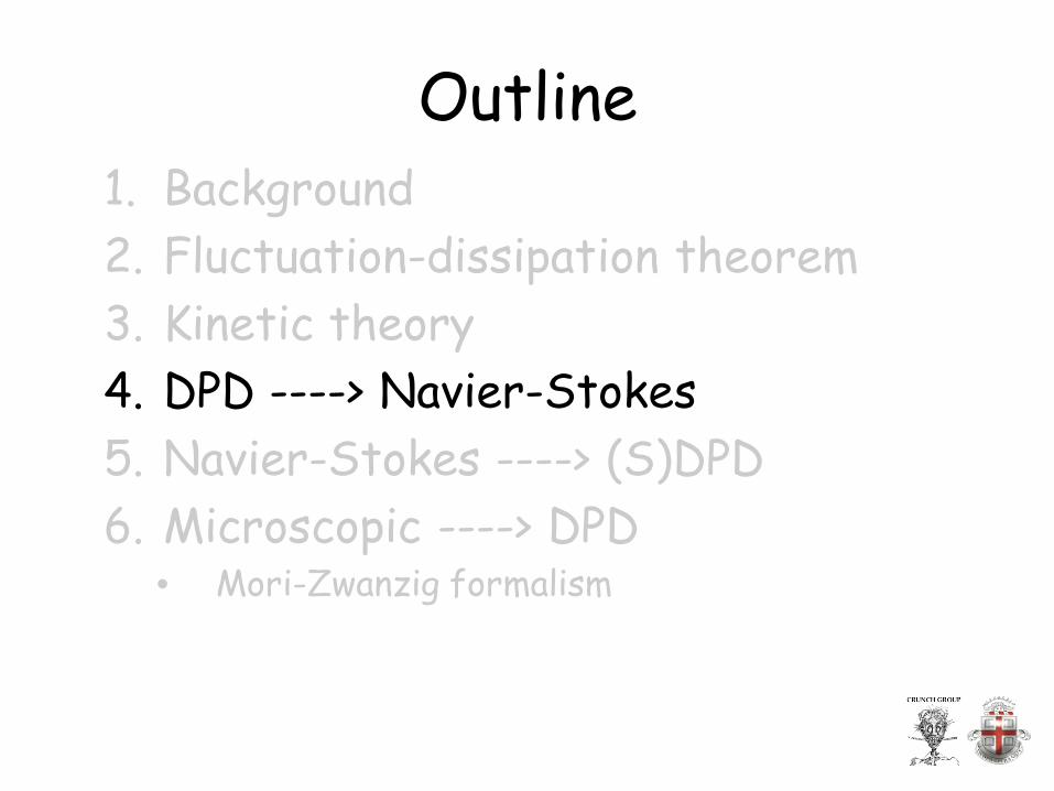
Outline 1. Background 2. Fluctuation-dissipation theorem 3. Kinetic theory 4. DPD ----> Navier-Stokes 5. Navier-Stokes ----> (S)DPD 6. Microscopic ----> DPD
• Mori-Zwanzig formalism
Outline 1. Background 2. Fluctuation-dissipation theorem 3. Kinetic theory 4. DPD ----> Navier-Stokes 5. Navier-Stokes ----> (S)DPD 6. Microscopic ----> DPD
• Mori-Zwanzig formalism
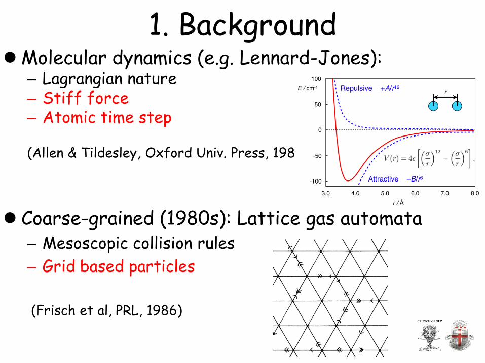
1. Background Molecular dynamics (e.g. Lennard-Jones):
– Lagrangian nature – Stiff force – Atomic time step
(Allen & Tildesley, Oxford Univ. Press, 1989)
Coarse-grained (1980s): Lattice gas automata – Mesoscopic collision rules – Grid based particles
(Frisch et al, PRL, 1986)
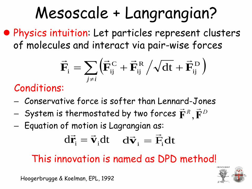
Physics intuition: Let particles represent clusters of molecules and interact via pair-wise forces
Conditions: – Conservative force is softer than Lennard-Jones – System is thermostated by two forces – Equation of motion is Lagrangian as:
dtd ii vr = dtFd ii
=v
Hoogerbrugge & Koelman, EPL, 1992
( )∑≠
++=ij
Dij
Rij
Ciji dt FFFF
Mesoscale + Langrangian?
This innovation is named as DPD method!
Outline 1. Background 2. Fluctuation-dissipation theorem 3. Kinetic theory 4. DPD ----> Navier-Stokes 5. Navier-Stokes ----> (S)DPD 6. Microscopic ----> DPD
• Mori-Zwanzig formalism
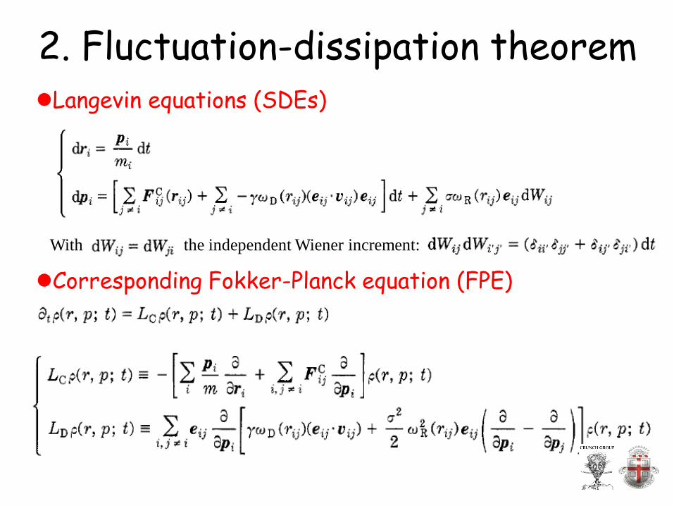
2. Fluctuation-dissipation theorem
Langevin equations (SDEs)
With the independent Wiener increment:
Corresponding Fokker-Planck equation (FPE)
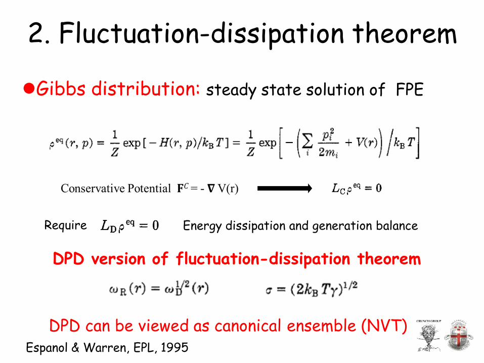
Gibbs distribution: steady state solution of FPE
DPD version of fluctuation-dissipation theorem
Require Energy dissipation and generation balance
DPD can be viewed as canonical ensemble (NVT)
2. Fluctuation-dissipation theorem
Espanol & Warren, EPL, 1995
Outline 1. Background 2. Fluctuation-dissipation theorem 3. kinetic theory 4. DPD ----> Navier-Stokes 5. Navier-Stokes ----> (S)DPD 6. Microscopic ----> DPD
• Mori-Zwanzig formalism
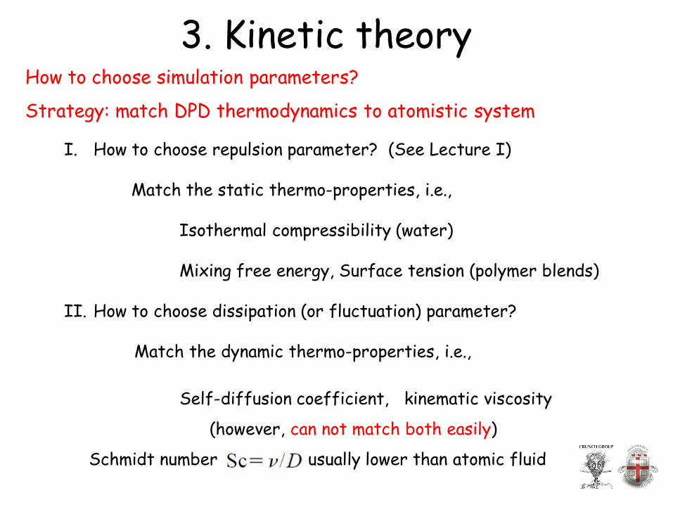
3. Kinetic theory How to choose simulation parameters?
Strategy: match DPD thermodynamics to atomistic system
I. How to choose repulsion parameter? (See Lecture I)
Match the static thermo-properties, i.e., Isothermal compressibility (water) Mixing free energy, Surface tension (polymer blends)
II. How to choose dissipation (or fluctuation) parameter? Match the dynamic thermo-properties, i.e., Self-diffusion coefficient, kinematic viscosity
(however, can not match both easily)
Schmidt number usually lower than atomic fluid
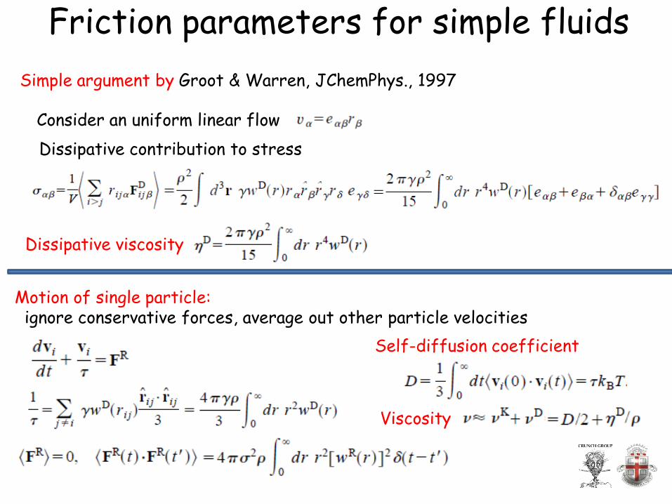
Friction parameters for simple fluids Simple argument by Groot & Warren, JChemPhys., 1997
Dissipative contribution to stress
Dissipative viscosity
Motion of single particle: ignore conservative forces, average out other particle velocities Self-diffusion coefficient
Viscosity
Consider an uniform linear flow
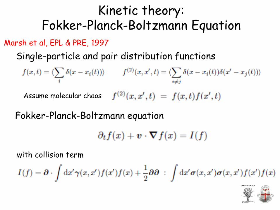
Marsh et al, EPL & PRE, 1997
with collision term
Single-particle and pair distribution functions
Fokker-Planck-Boltzmann equation
Kinetic theory: Fokker-Planck-Boltzmann Equation
Assume molecular chaos
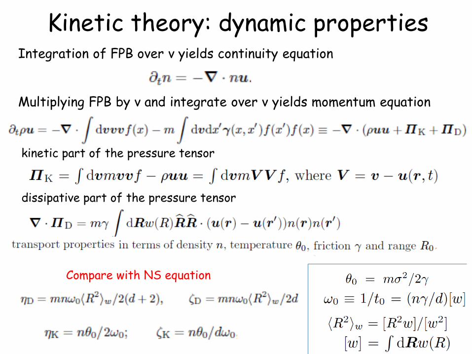
Integration of FPB over v yields continuity equation
Multiplying FPB by v and integrate over v yields momentum equation
Compare with NS equation
Kinetic theory: dynamic properties
kinetic part of the pressure tensor
dissipative part of the pressure tensor
Outline 1. Background 2. Fluctuation-dissipation theorem 3. Kinetic theory 4. DPD ----> Navier-Stokes 5. Navier-Stokes ----> (S)DPD 6. Microscopic ----> DPD
• Mori-Zwanzig formalism
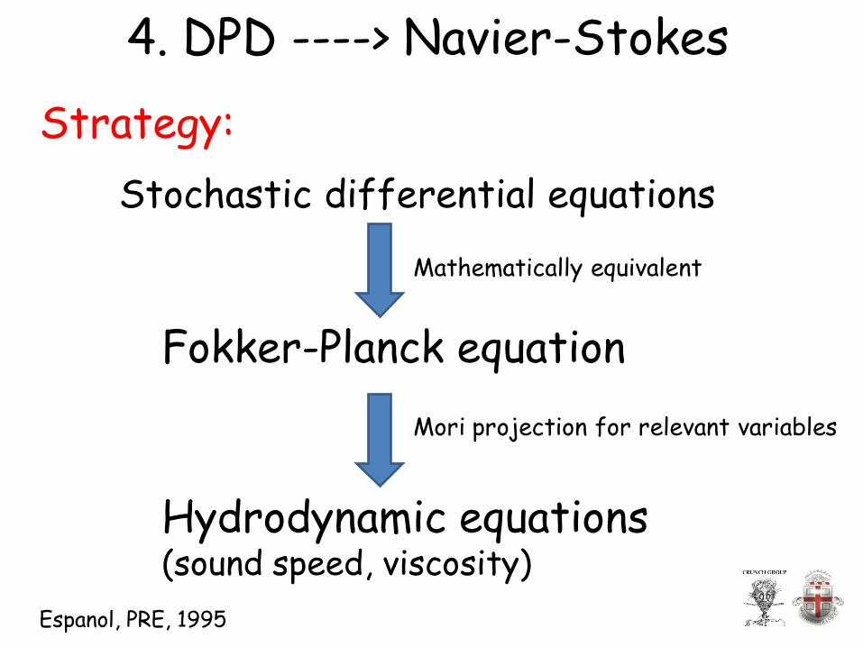
4. DPD ----> Navier-Stokes
Stochastic differential equations
Fokker-Planck equation
Mathematically equivalent
Mori projection for relevant variables
Espanol, PRE, 1995
Hydrodynamic equations (sound speed, viscosity)
Strategy:
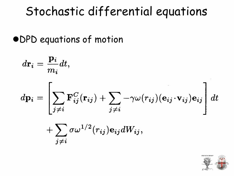
Stochastic differential equations
DPD equations of motion
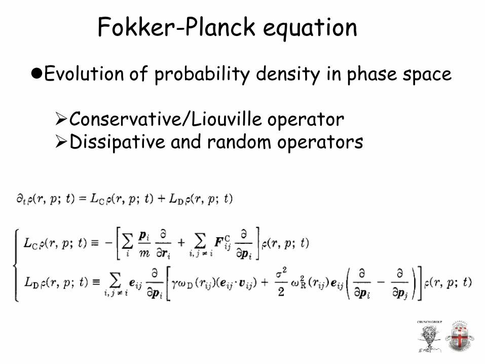
Fokker-Planck equation
Evolution of probability density in phase space Conservative/Liouville operator Dissipative and random operators
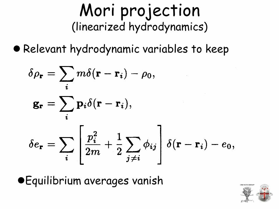
Mori projection (linearized hydrodynamics)
Relevant hydrodynamic variables to keep
Equilibrium averages vanish
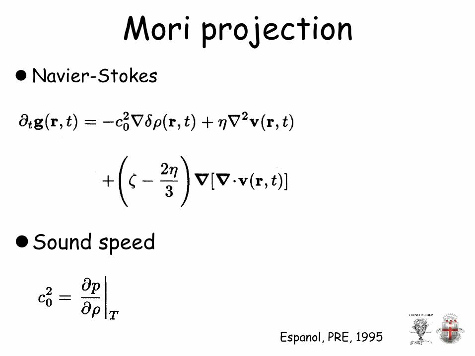
Mori projection Navier-Stokes
Sound speed
Espanol, PRE, 1995
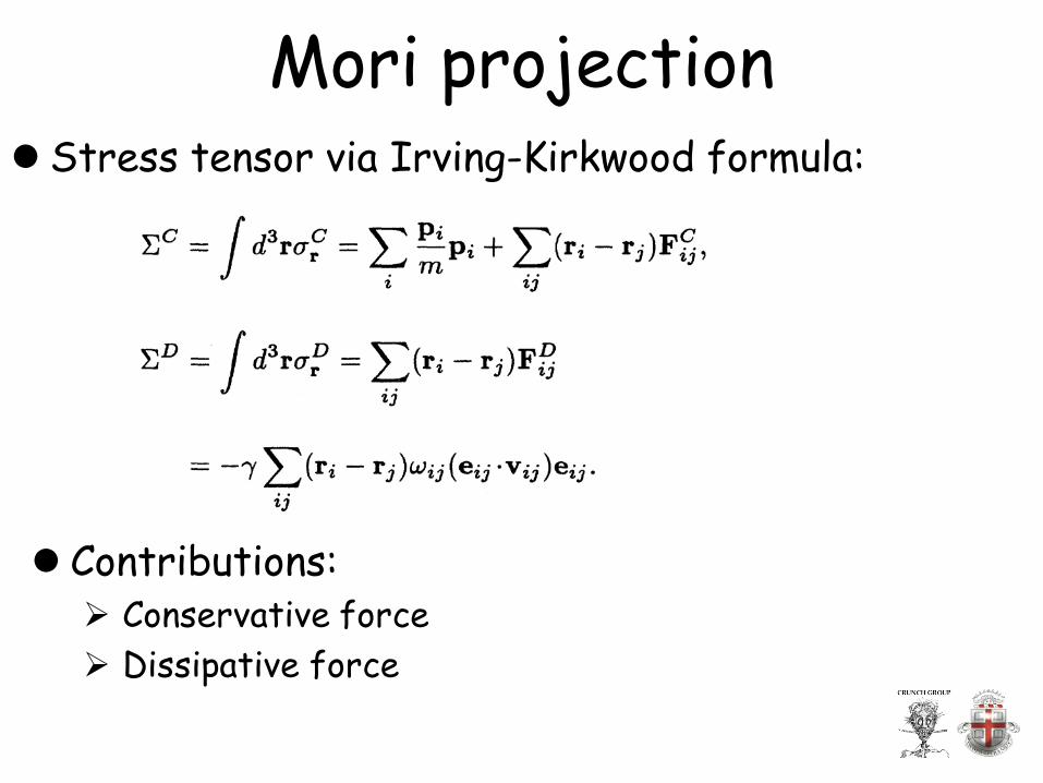
Mori projection Stress tensor via Irving-Kirkwood formula:
Contributions: Conservative force Dissipative force
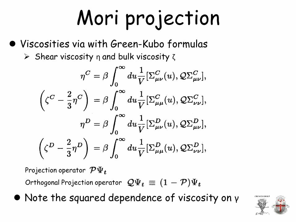
Mori projection Viscosities via with Green-Kubo formulas
Shear viscosity η and bulk viscosity ζ
Note the squared dependence of viscosity on γ
Projection operator
Orthogonal Projection operator
Outline 1. Background 2. Fluctuation-dissipation theorem 3. Kinetic theory 4. DPD ----> Navier-Stokes 5. Navier-Stokes ----> (S)DPD 6. Microscopic ----> DPD
• Mori-Zwanzig formalism
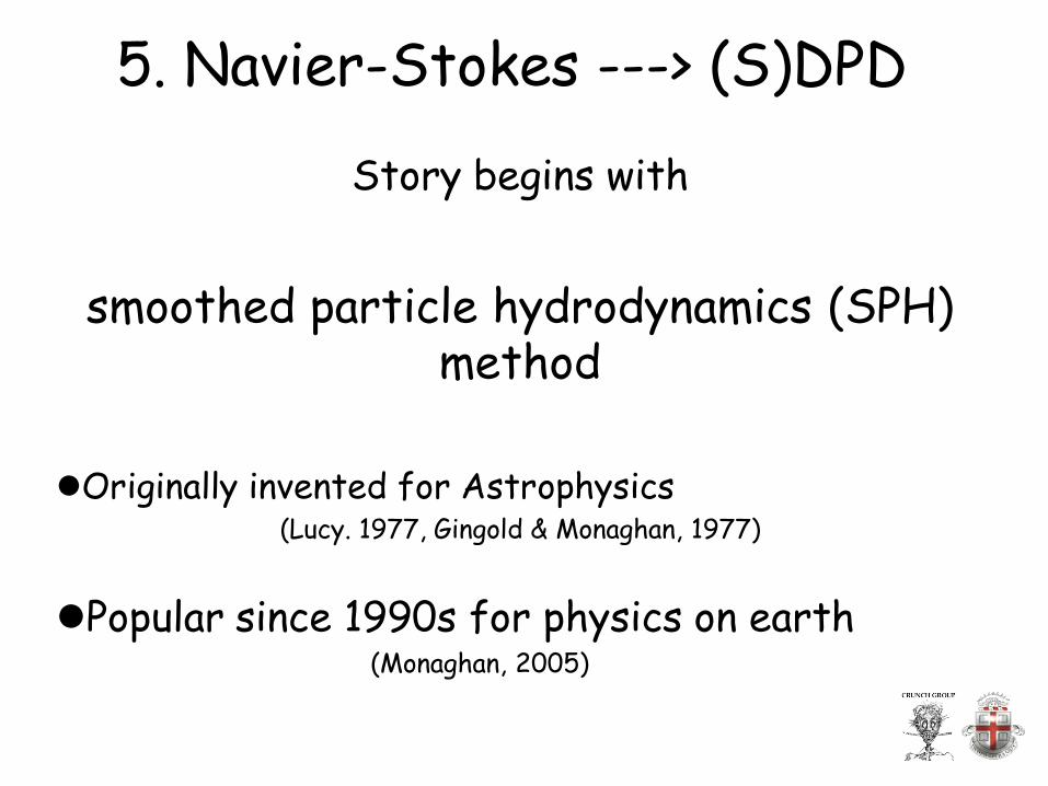
Story begins with
smoothed particle hydrodynamics (SPH) method
Originally invented for Astrophysics
(Lucy. 1977, Gingold & Monaghan, 1977)
Popular since 1990s for physics on earth (Monaghan, 2005)
5. Navier-Stokes ---> (S)DPD
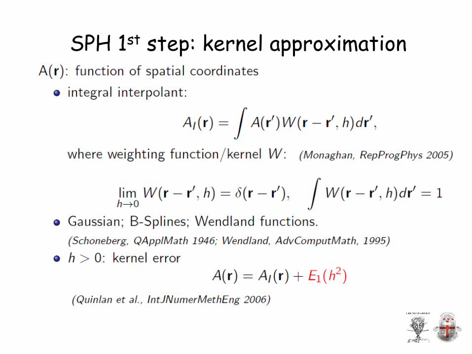
SPH 1st step: kernel approximation
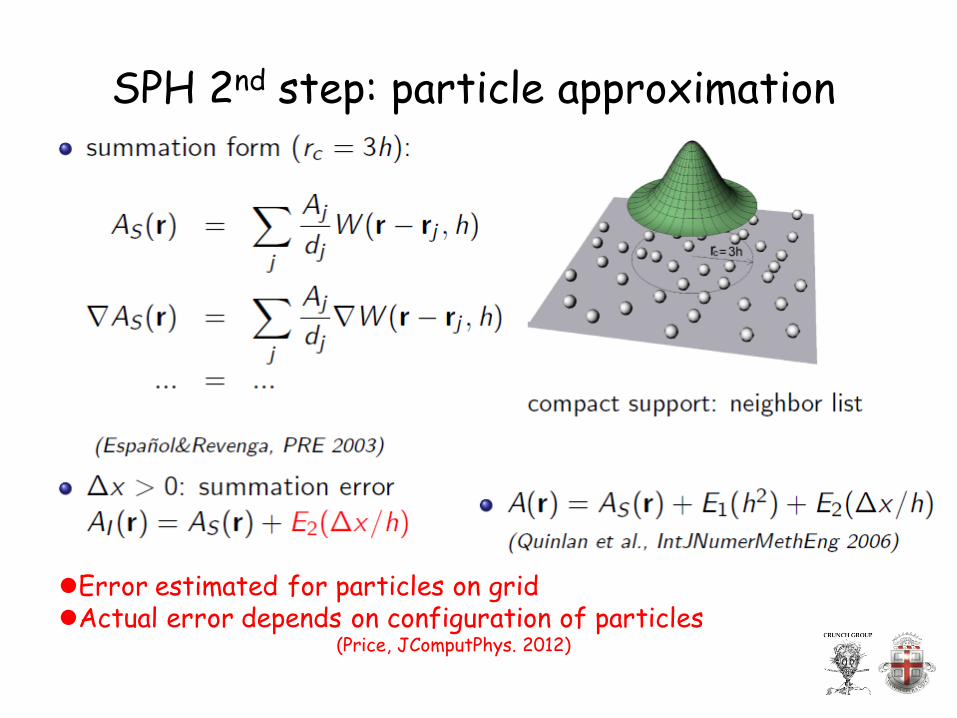
SPH 2nd step: particle approximation
Error estimated for particles on grid Actual error depends on configuration of particles
(Price, JComputPhys. 2012)
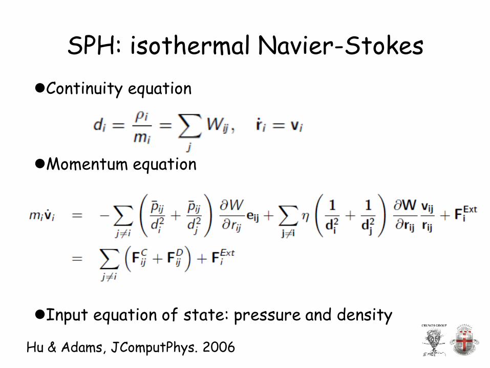
SPH: isothermal Navier-Stokes Continuity equation
Momentum equation
Input equation of state: pressure and density
Hu & Adams, JComputPhys. 2006
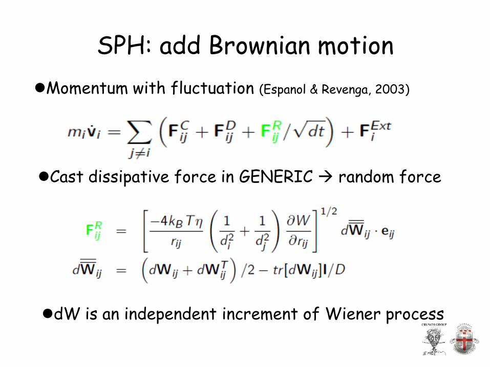
SPH: add Brownian motion Momentum with fluctuation (Espanol & Revenga, 2003)
Cast dissipative force in GENERIC random force
dW is an independent increment of Wiener process
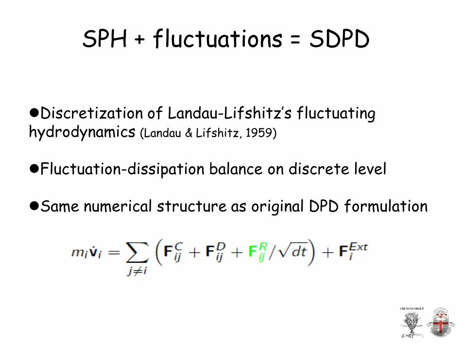
SPH + fluctuations = SDPD
Discretization of Landau-Lifshitz’s fluctuating hydrodynamics (Landau & Lifshitz, 1959)
Fluctuation-dissipation balance on discrete level
Same numerical structure as original DPD formulation
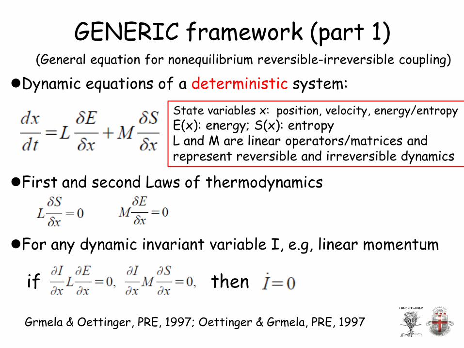
GENERIC framework (part 1) (General equation for nonequilibrium reversible-irreversible coupling)
Grmela & Oettinger, PRE, 1997; Oettinger & Grmela, PRE, 1997
Dynamic equations of a deterministic system: State variables x: position, velocity, energy/entropy E(x): energy; S(x): entropy L and M are linear operators/matrices and represent reversible and irreversible dynamics
First and second Laws of thermodynamics
For any dynamic invariant variable I, e.g, linear momentum
if then
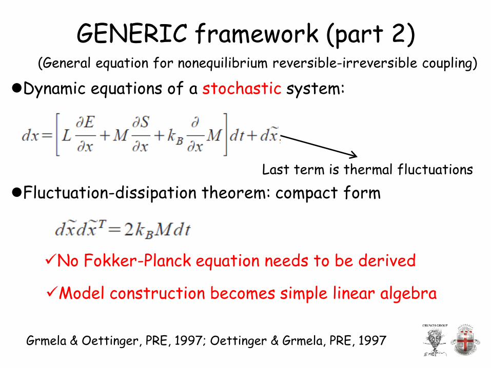
GENERIC framework (part 2) (General equation for nonequilibrium reversible-irreversible coupling)
Dynamic equations of a stochastic system:
Fluctuation-dissipation theorem: compact form
No Fokker-Planck equation needs to be derived
Last term is thermal fluctuations
Model construction becomes simple linear algebra
Grmela & Oettinger, PRE, 1997; Oettinger & Grmela, PRE, 1997
Outline 1. Background 2. Fluctuation-dissipation theorem 3. Kinetic theory 4. DPD ----> Navier-Stokes 5. Navier-Stokes ----> (S)DPD 6. Microscopic ----> DPD
• Mori-Zwanzig formalism
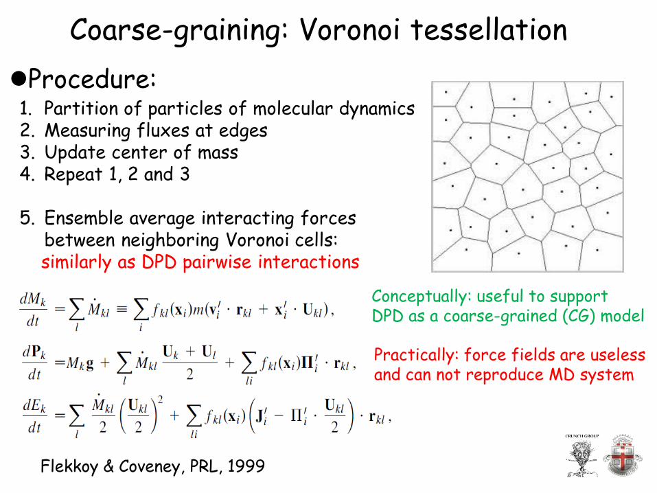
Coarse-graining: Voronoi tessellation
1. Partition of particles of molecular dynamics 2. Measuring fluxes at edges 3. Update center of mass 4. Repeat 1, 2 and 3
5. Ensemble average interacting forces
between neighboring Voronoi cells: similarly as DPD pairwise interactions
Conceptually: useful to support DPD as a coarse-grained (CG) model
Practically: force fields are useless and can not reproduce MD system
Procedure:
Flekkoy & Coveney, PRL, 1999
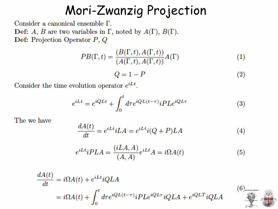
Mori-Zwanzig Projection
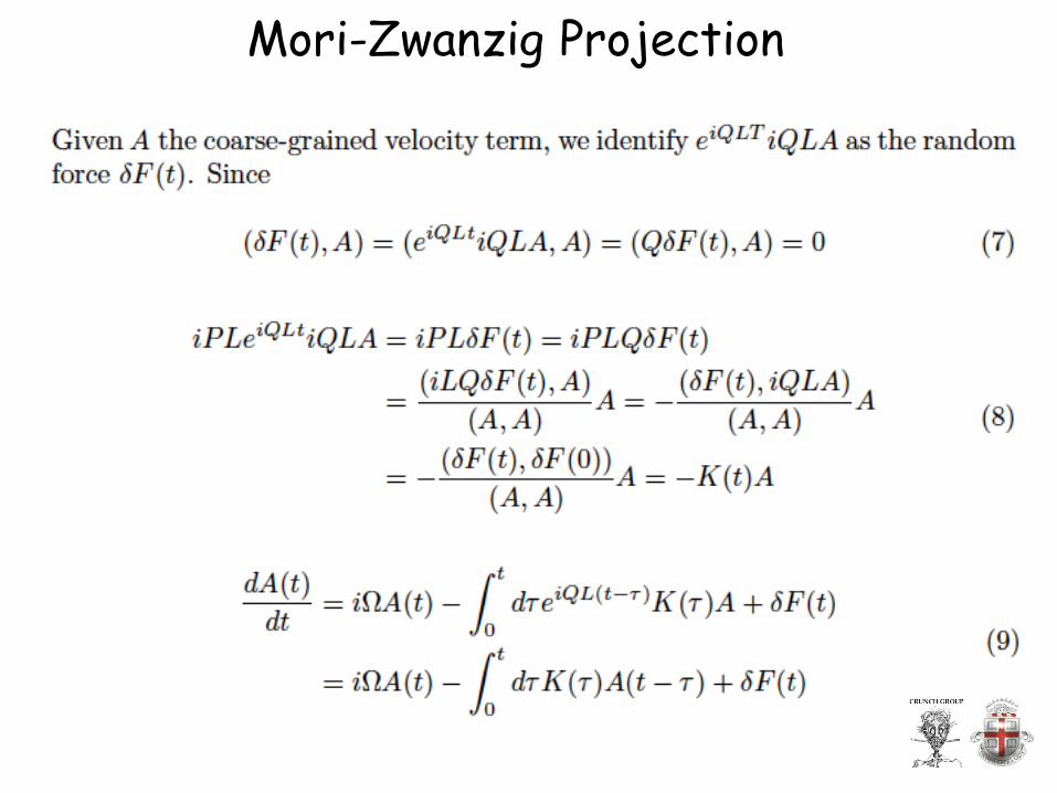
Mori-Zwanzig Projection
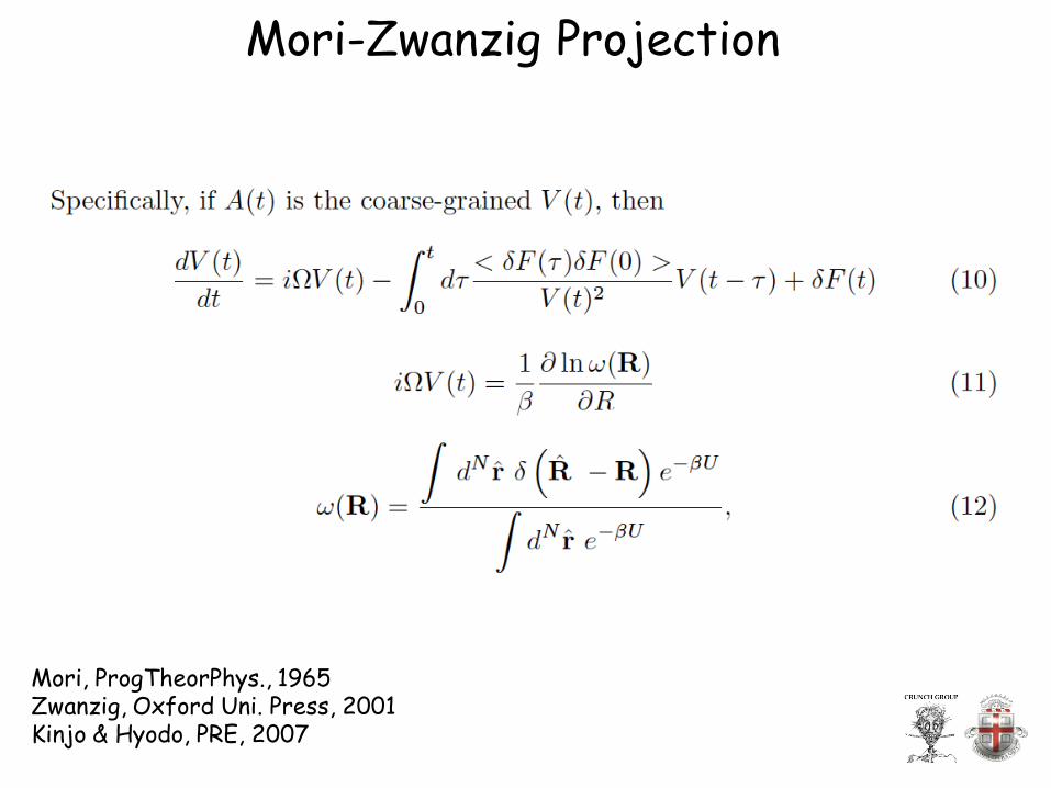
Mori-Zwanzig Projection
Mori, ProgTheorPhys., 1965 Zwanzig, Oxford Uni. Press, 2001 Kinjo & Hyodo, PRE, 2007
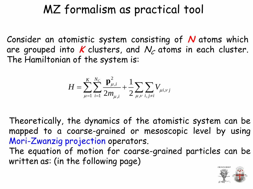
Consider an atomistic system consisting of N atoms which are grouped into K clusters, and NC atoms in each cluster. The Hamiltonian of the system is:
2,
,1 1 , ,,
12 2
CNKi
i ji i j ii
H Vmµ
µ νµ µ νµ= = ≠
= +∑∑ ∑∑p
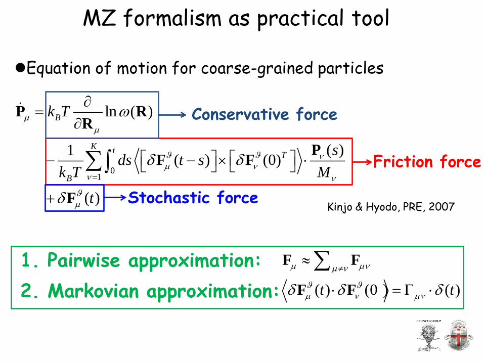
Theoretically, the dynamics of the atomistic system can be mapped to a coarse-grained or mesoscopic level by using Mori-Zwanzig projection operators. The equation of motion for coarse-grained particles can be written as: (in the following page)
MZ formalism as practical tool
01
ln ( )
( )1 ( ) (0)
( )
B
K t T
B
k T
sds t sk T M
t
µµ
ϑ ϑ νµ ν
ν ν
ϑµ
ω
δ δ
δ=
∂=
∂
− − × ⋅
+
∑∫
P RR
PF F
F
Kinjo & Hyodo, PRE, 2007
Friction force
Conservative force
Stochastic force
1. Pairwise approximation: 2. Markovian approximation:
µ µνµ ν≠≈∑F F
( ) (0 ) ( )t tϑ ϑµ ν µνδ δ δ⋅ = Γ ⋅F F
MZ formalism as practical tool
Equation of motion for coarse-grained particles
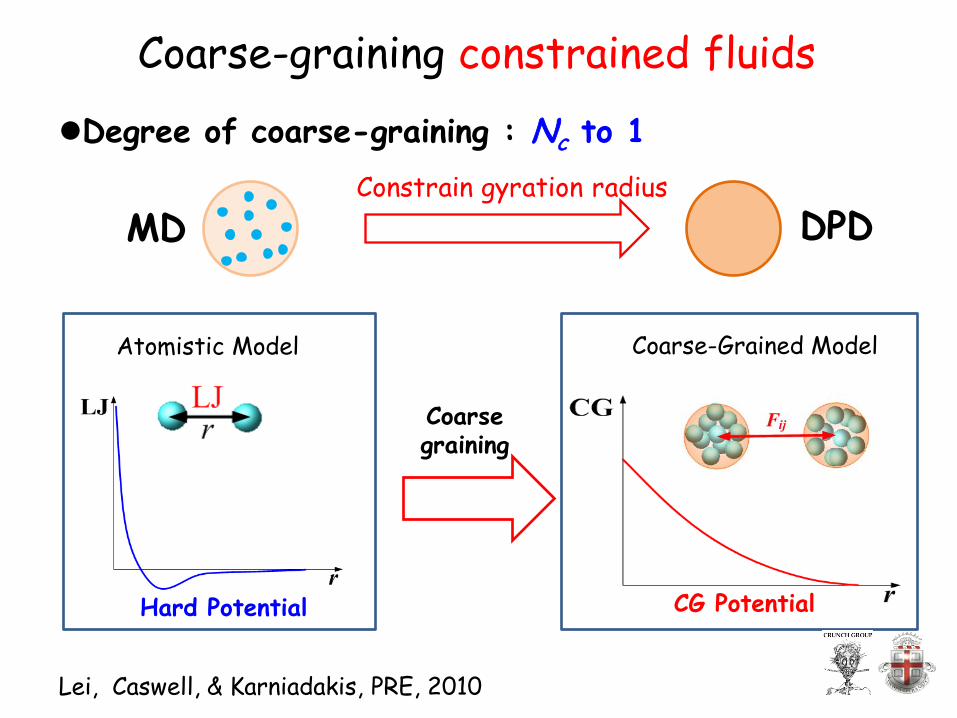
Coarse-graining constrained fluids
DPD
Atomistic Model Coarse-Grained Model
Hard Potential CG Potential
Coarse graining
Degree of coarse-graining : Nc to 1
MD
Lei, Caswell, & Karniadakis, PRE, 2010
Constrain gyration radius
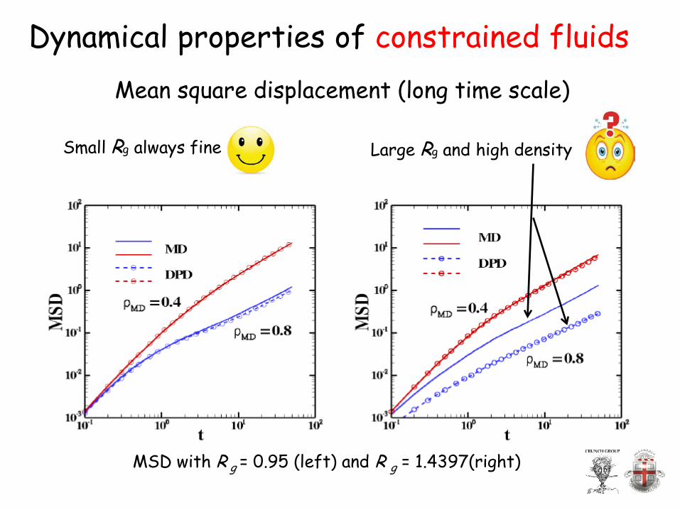
Dynamical properties of constrained fluids Mean square displacement (long time scale)
MSD with R g = 0.95 (left) and R g = 1.4397(right)
Small Rg always fine Large Rg and high density
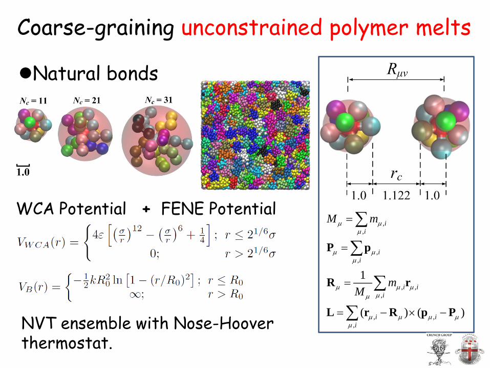
WCA Potential + FENE Potential
NVT ensemble with Nose-Hoover thermostat.
,,
,,
, ,,
, ,,
1
( ) ( )
ii
ii
i ii
i ii
M m
mM
µ µµ
µ µµ
µ µ µµµ
µ µ µ µµ
=
=
=
= − × −
∑
∑
∑
∑
P p
R r
L r R p P
Coarse-graining unconstrained polymer melts
Natural bonds
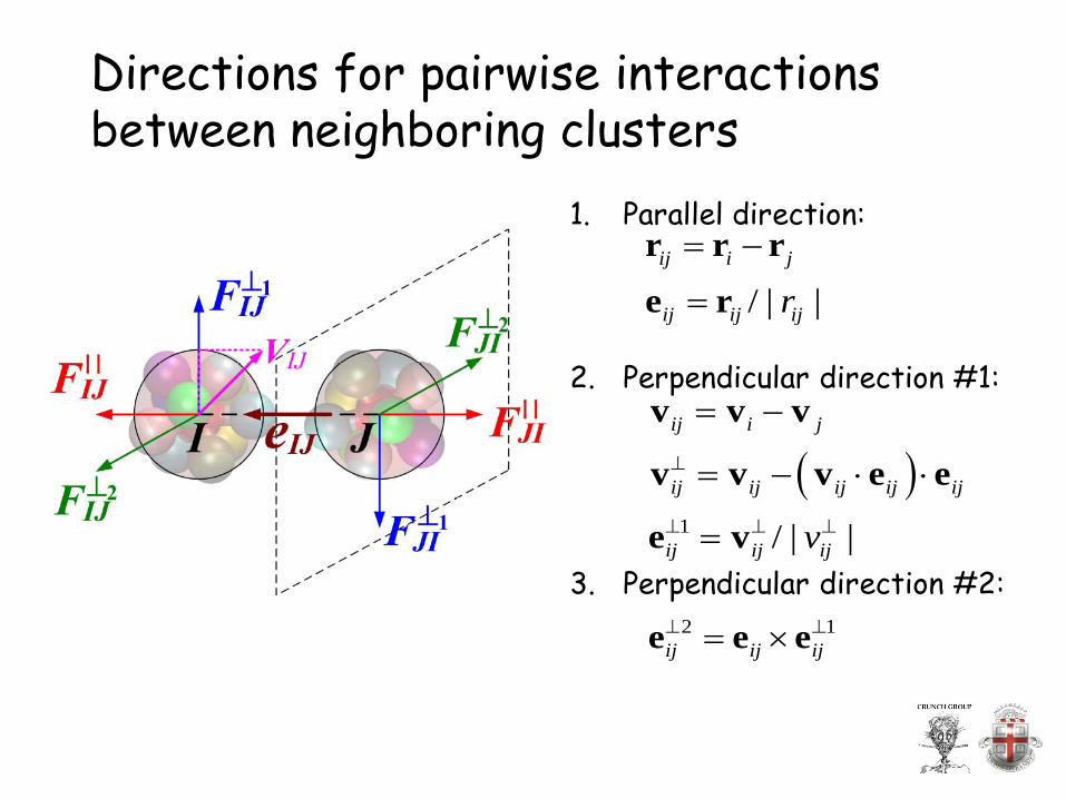
Directions for pairwise interactions between neighboring clusters
1. Parallel direction:
2. Perpendicular direction #1:
3. Perpendicular direction #2:
/ | |ij i j
ij ij ijr= −
=
r r re r
( )1 / | |
ij i j
ij ij ij ij ij
ij ij ijv
⊥
⊥ ⊥ ⊥
= −
= − ⋅ ⋅
=
v v v
v v v e e
e v
2 1ij ij ij⊥ ⊥= ×e e e
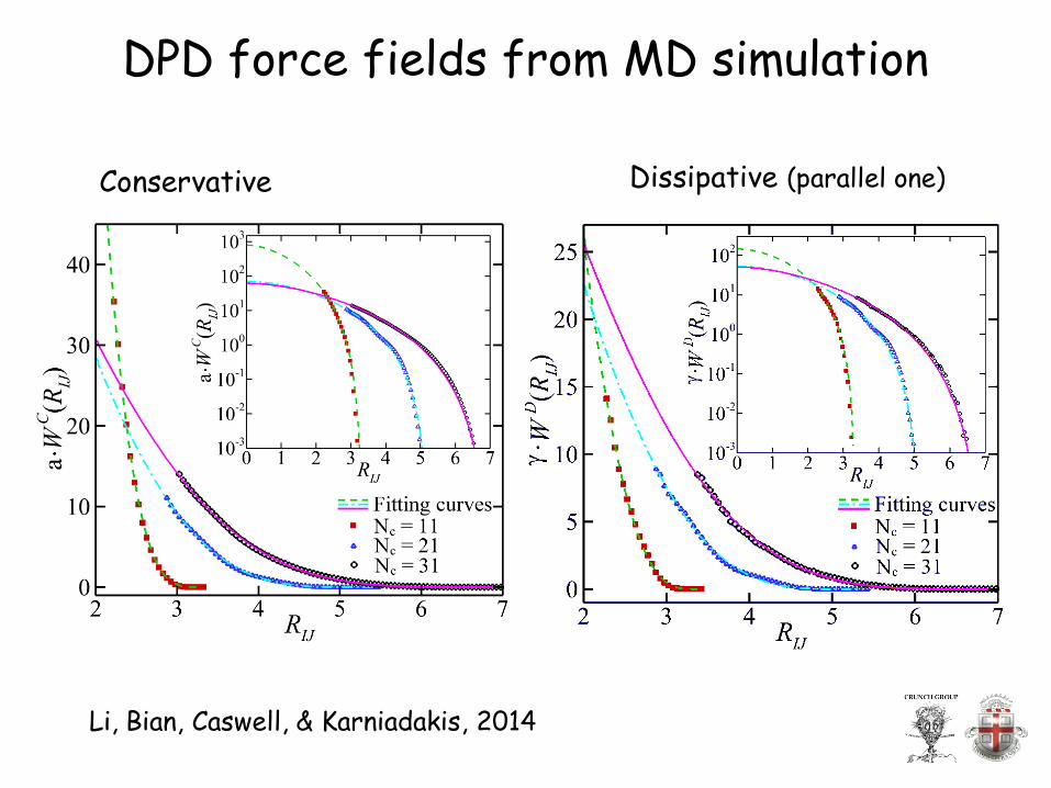
DPD force fields from MD simulation
Conservative Dissipative (parallel one)
Li, Bian, Caswell, & Karniadakis, 2014
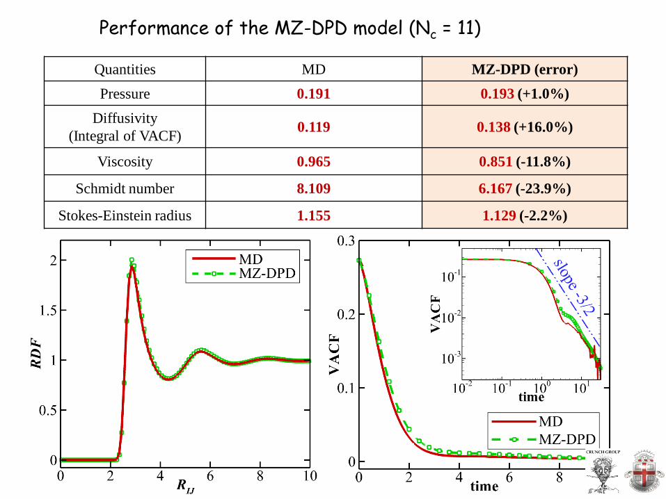
Quantities MD MZ-DPD (error) Pressure 0.191 0.193 (+1.0%)
Diffusivity (Integral of VACF) 0.119 0.138 (+16.0%)
Viscosity 0.965 0.851 (-11.8%)
Schmidt number 8.109 6.167 (-23.9%)
Stokes-Einstein radius 1.155 1.129 (-2.2%)
Performance of the MZ-DPD model (Nc = 11)
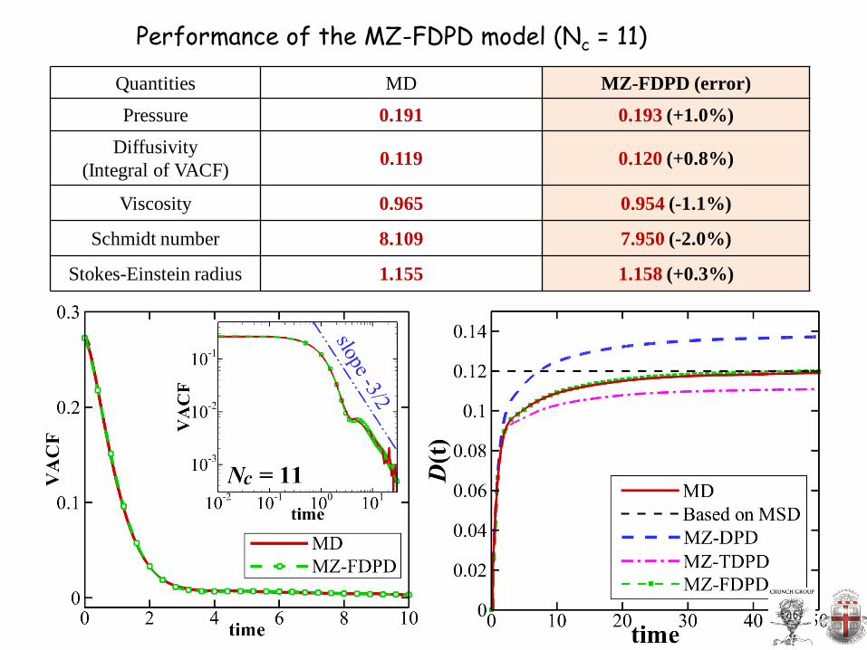
Quantities MD MZ-FDPD (error) Pressure 0.191 0.193 (+1.0%)
Diffusivity (Integral of VACF) 0.119 0.120 (+0.8%)
Viscosity 0.965 0.954 (-1.1%)
Schmidt number 8.109 7.950 (-2.0%)
Stokes-Einstein radius 1.155 1.158 (+0.3%)
Performance of the MZ-FDPD model (Nc = 11)
Conclusion & Outlook • Invented by physics intuition • Statistical physics on solid ground
– Fluctuation-dissipation theorem – Canonical ensemble (NVT)
• DPD <-----> Navier-Stokes equations • Coarse-graining microscopic system
– Mori-Zwanzig formalism