A SYSTEMATIC STUDY OF DEEP GENERATIVE MODELS FOR …

1 Copyright © 2020 by ASME

Data Driven Design EDSGN/IE 561

Spring 2020, University Park, Pennsylvania, USA

A SYSTEMATIC STUDY OF DEEP GENERATIVE MODELS FOR RAPID

TOPOLOGY OPTIMIZATION

Akash Agrawal Engineering Design

The Pennsylvania State University State College, PA, USA

Manoj Malviya Mechanical Engineering

The Pennsylvania State University State College, PA, USA

Pranjali Yadav Industrial Engineering

The Pennsylvania State University

State College, PA, USA

Yu-Hao Chang Industrial Engineering



Dr. Christopher McComb Engineering Design



KEYWORDS Topology Optimization, Generative Algorithm,

Machine Learning, Computational Design

SUMMARY

With the advent in Additive Manufacturing (AM)

technologies and Computational Sciences, design

algorithms such as Topology Optimization (TO) have

garnered the interest of academia and industry. TO

aims to generate optimum structures by maximizing

the stiffness of the structure, given a set of geometric,

loading and boundary conditions. However, these

approaches are computationally expensive as it

requires a large number of iterations to converge to

an optimum solution. The purpose of this work is to

explore the effectiveness of deep generative models on

a diverse range of topology optimization problems

with varying design constraints, loading and

boundary conditions. Specifically, four distinctive

models were successfully developed, trained, and

evaluated to generate rapid designs with comparable

results to that of conventional algorithms. Our

findings highlight the effectiveness of the novel design

problem representation and proposed generative

models in rapid topology optimization.

1. INTRODUCTION

Structural optimization is a process of determining the

optimum design variables mathematically for a set of

constraints and objectives. These algorithms use

gradient based algorithms to explore design solutions

and eventually converge at globally optimum

solutions. In the case of non-analytical objective

functions or heavy-computational models,

researchers implemented meta-models for quicker

convergence [1].

Topology Optimization (TO), a computational design

approach initially proposed in [2], finds an optimum

material distribution for maximizing the stiffness of

structure for a user-specified constraint on volume

distribution. These algorithms result in an organic

structure suitable for the AM process and thus heavily

influence the design process. Solid Isotropic Material

Penalization (SIMP) [3], is the most used algorithm to

find the optimum material distribution (see Figure 1).


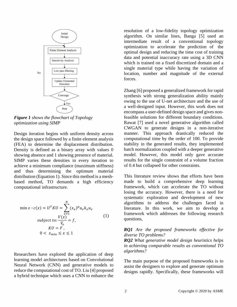
Figure 1 shows the flowchart of Topology

optimization using SIMP

Design iteration begins with uniform density across

the design space followed by a finite element analysis

(FEA) to determine the displacement distribution.

Density is defined as a binary array with values 0

showing absence and 1 showing presence of material.

SIMP varies these densities in every iteration to

achieve a minimum compliance (maximum stiffness)

and thus determining the optimum material

distribution (Equation 1). Since this method is a mesh-

based method, TO demands a high efficiency

computational infrastructure.

min 𝑥 ∶ 𝑐(𝑥) = 𝑈𝑇𝐾𝑈 = ∑(𝑥𝑒)𝑝𝑢𝑒𝑘𝑜𝑢𝑒

𝑁

𝑒=1

𝑠𝑢𝑏𝑗𝑒𝑐𝑡 𝑡𝑜:𝑉(𝑥)

𝑉𝑜= 𝑓,

𝐾𝑈 = 𝐹 , 0 < 𝑥𝑚𝑖𝑛 ≤ 𝑥 ≤ 1

(1)

Researchers have explored the application of deep

learning model architectures based on Convolutional

Neural Network (CNN) and generative models to

reduce the computational cost of TO. Liu [4] proposed

a hybrid technique which uses a CNN to enhance the

resolution of a low-fidelity topology optimization

algorithm. On similar lines, Banga [5] used an

intermediate result of a conventional topology

optimization to accelerate the prediction of the

optimal design and reducing the time cost of training

data and potential inaccuracy rate using a 3D CNN

which is trained on a fixed discretized domain and a

single material type while having the variation of

location, number and magnitude of the external

forces.

Zhang [6] proposed a generalized framework for rapid

synthesis with strong generalization ability mainly

owing to the use of U-net architecture and the use of

a well-designed input. However, this work does not

encompass a user-defined design space and gives non-

feasible solutions for different boundary conditions.

Rawat [7] used a novel generative algorithm called

CWGAN to generate designs in a non-iterative

manner. This approach drastically reduced the

computational time by the order of 100. To provide

stability in the generated results, they implemented

batch normalization coupled with a deeper generative

model. However, this model only gave accurate

results for the single constraint of a volume fraction

of 0.4 but collapsed for other constraints.

This literature review shows that efforts have been

made to build a comprehensive deep learning

framework, which can accelerate the TO without

losing the accuracy. However, there is a need for

systematic exploration and development of new

algorithms to address the challenges faced in

literature. In this work, we aim to develop a

framework which addresses the following research

questions,

RQ1 Are the proposed frameworks effective for

diverse TO problems?

RQ2 What generative model design heuristics helps

in achieving comparable results as conventional TO

algorithms?

The main purpose of the proposed frameworks is to

assist the designers to explore and generate optimum

designs rapidly. Specifically, these frameworks will


drastically reduce the design cycle time without

compromising the solution accuracy and designer’s

freedom. Therefore, this framework has a direct

impact on AM and Mass Customization focused

organizations providing monetary benefits.

Additionally, this framework can be modified and

implemented in academia for teaching design in a

real-time environment, where students can learn the

fundamental concepts of design and get rapid

feedback.

The rest of the paper is organized as follows. Section

2 provides an insight into the methodology adopted

for generation and representation of the dataset with

varying geometric, boundary and loading conditions.

Moreover, data augmentation techniques to improve

the representation without changing the semantics of

the data are discussed. The architecture and learning

details of the four generative models are elaborated in

Section 3 followed by detailed results in Section 4.

Section 5 discusses the efficacy of all the frameworks

and elaborates potential for future work. Section 6

concludes the paper with a summary of the

effectiveness of deep generative models for rapid

topology optimization.

2. DATASET

The work investigates an additively manufactured

Michell beam as a use case for the proposed deep

learning framework. We implemented the SIMP

model topology optimization to generate a training

dataset with N number of samples. Literature

suggests that the number of samples N should be

around 4000-80000 but varies based on the model

architecture and problem complexity. We generated

60,000 data points considering different boundary

(BC) and loading conditions (LC), geometric

constraints, and volume fraction (VF). The rest of the

section is organized as follows. First, we show

different conditions and constraints used for dataset

generation (Section 2.1). Second, we present the

representation of problems as images (Section 2.2).

Third, we discuss the data augmentation techniques

we applied for better accuracy (Section 2.3).

2.1 Generating Diverse Training Data

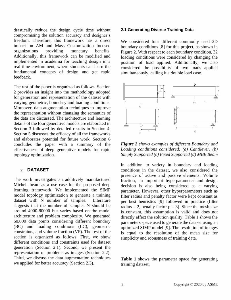
We considered four different commonly used 2D

boundary conditions [8] for this project, as shown in

Figure 2. With respect to each boundary condition, 32

loading conditions were considered by changing the

position of load applied. Additionally, we also

considered the possibility of two loads applied

simultaneously, calling it a double load case.

Figure 2 shows examples of different Boundary and

Loading conditions considered: (a) Cantilever, (b)

Simply Supported (c) Fixed Supported (d) MBB Beam

In addition to variety in boundary and loading

conditions in the dataset, we also considered the

presence of active and passive elements. Volume

fraction, an important hyperparameter and design

decision is also being considered as a varying

parameter. However, other hyperparameters such as

filter radius and penalty factor were kept constant as

per best heuristics [9] followed in practice (filter

radius = 2, penalty factor p = 3). Since the mesh size

is constant, this assumption is valid and does not

directly affect the solution quality. Table 1 shows the

parameters space used to generate the dataset using an

optimized SIMP model [9]. The resolution of images

is equal to the resolution of the mesh size for

simplicity and robustness of training data.

Table 1 shows the parameter space for generating

training dataset.


Variable Range/

Options

Total

Number

Volume Fraction 0.25-0.75 10

Boundary Conditions (1)

Cantilever

(2) Simply

Supported

(3) Fixed

Support

(4) MBB

Beam

32X4 =

128

(single

load)

32X32X4

= 4096

(double

loads)

Loading

Condition

Load

Direction

Magnitude -10 to 10

except 0 5

Geometric

Constraints

radii 4-8 10

location (10,10) to

(53,21) 100

case

Active,

Passive,

Blank

element

3

As presented above in Table 1, 3.84 million single and

122.8 million double load cases are possible.

However, not the entire dataset is needed to train a

good network. Therefore, we randomly selected

30,000 for single and 30,000 double load cases and

generated solutions. This splitting resulted in a

diverse training dataset and therefore, improving the

versatility of proposed networks if trained properly.

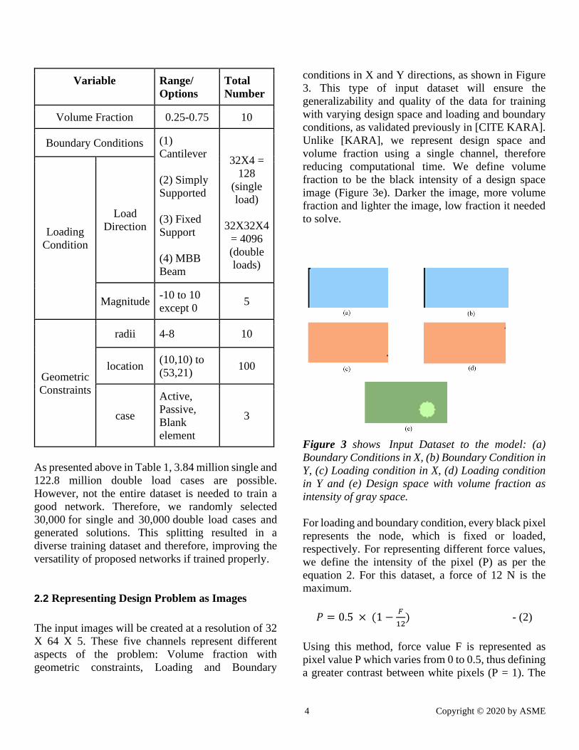
2.2 Representing Design Problem as Images

The input images will be created at a resolution of 32

X 64 X 5. These five channels represent different

aspects of the problem: Volume fraction with

geometric constraints, Loading and Boundary

conditions in X and Y directions, as shown in Figure

3. This type of input dataset will ensure the

generalizability and quality of the data for training

with varying design space and loading and boundary

conditions, as validated previously in [CITE KARA].

Unlike [KARA], we represent design space and

volume fraction using a single channel, therefore

reducing computational time. We define volume

fraction to be the black intensity of a design space

image (Figure 3e). Darker the image, more volume

fraction and lighter the image, low fraction it needed

to solve.

Figure 3 shows Input Dataset to the model: (a)

Boundary Conditions in X, (b) Boundary Condition in

Y, (c) Loading condition in X, (d) Loading condition

in Y and (e) Design space with volume fraction as

intensity of gray space.

For loading and boundary condition, every black pixel

represents the node, which is fixed or loaded,

respectively. For representing different force values,

we define the intensity of the pixel (P) as per the

equation 2. For this dataset, a force of 12 N is the

maximum.

𝑃 = 0.5 × (1 −𝐹

12) - (2)

Using this method, force value F is represented as

pixel value P which varies from 0 to 0.5, thus defining

a greater contrast between white pixels (P = 1). The


output of the deep learning network are grayscale

images that have been generated using the

conventional SIMP model. Figure 4 shows output

examples for each boundary conditions, outputted

from SIMP 88 lines tool.

(a) BC 1, Load 1 (b) BC 2, Load 2

(c) Active Element (d) Passive Element

Figure 4 shows the Output Images obtained using

the SIMP Topology Optimization model for various

initial design problems (a-d)

2.3 Data Augmentation for improving learning

Convolutional deep neural networks are the model

that performs good learning of the feature especially

on many computer vision problems. However, it

might face some potential problems that affect the

performance of model learning, for example, the size

of the training data set. If the data size is not broad and

big enough to encompass the variance of the object,

the deep learning model tends to overfit. To avoid

overfitting, several techniques of data augmentation

could be applied in our work to enhance the learning

performance. The first technique we applied is

random sampling. It is widely used to randomly

choose the unseen data set to validate the trained

model in each epoch, the commonly known as cross

validation. It can avoid overfitting in the same dataset

comparatively.

Secondly, the accuracy of the neural network model

is computed by the stochastic gradient descent (SGD)

optimization. In the research of Hoffer et al. (2017)

points out the quality of the model depends on the

number of SGD iterations and the number of batch

sizes. Therefore, in each batch of the model, SGD is

going to optimize the loss of each batch in the training

data sets, which means it can learn the feature

iteratively. In the meantime, better accuracy will be

obtained, and the weights of the network will be

adjusted to improve the performance of the model

since the training data size will be divided into

random batches for every epoch. On the other hand,

adopting less batch size can reduce the requirement of

memory to complete the stochastic gradient descent

convergence since it is computation expensive to

optimize the gradient over the entire dataset.

Third technique is applying gaussian blur to the

channels representing loading and boundary

conditions before feeding into our models. For

instance, the training images representation of the

loading condition, there is a single white spot on the

entire black image to show the location loading force

on the object. To allow the convolution layer to

extract this import feature from the image, especially

the low-level information, we used gaussian function

as the equation 3 to magnify the importance of the

feature, i.e. the white spot on the images. The 𝜇 and

𝜎 in the gaussian function are represented expected

value and variance respectively.

𝑔(𝑥) =1

𝜎√2𝜋𝑒

−1

2(

𝑥−𝜇

𝜎)2

(3)

Using this function, the model can learn the feature of

white spot of the loading location that is enforced by

gaussian blur as Figure 5 showed. We also inverted

the color of feeding images while loading to the

model, which obtained more black content. The

method is using 255 subtract every pixel value on the

images to represent the important features of images

by pixel value P = 1.


Figure 5: Loading condition representation after

adopting Gaussian blur and inverse of image.

The last approach we applied is the normalization of

training images. We normalized the training images

for GAN models from -1 to 1 and for CNN models

from 0 to 1. This normalization results in a faster

convergence due to smaller range to predict.

3. METHODOLOGY

The proposed methodology utilizes images as the raw

state for both the input and output data. Convolutions

are powerful feature extractors for image-based

problems. By detecting low level features and using

them to detect high level features makes them

powerful and efficient with image data. Thereby, four

distinctive deep generative frameworks based on

convolutional layers are proposed: TOP-CNN, a CNN

based regression framework, U-NET, a U shaped

framework and two GAN based frameworks, TOP-

GAN and DC-GAN Section 3.1, 3.2 and 3.3 details

the architecture and learning methodology of these

networks respectively.

3.1 Convolutional Neural Networks as generative models

Convolutional Neural Networks (CNNs) are neural

networks consisting of convolutional layers, max

pooling layers and fully connected layers that

demonstrate excellent performance in Image & Video

recognition, Image Analysis & Classification, Media

Recreation, Recommendation Systems, Natural

Language Processing. Specifically, for image

processing tasks, they are capable of assigning

importance to various aspects in the image. Moreover,

the preprocessing required in a CNN is much lower as

compared to other primitive methods in which

characteristics are hand-engineered, with enough

training. CNN based architectures like LeNet,

AlexNet, VGGNet, GoogLeNet, ResNet, ZFNet have

been key in building many state-of-the-art algorithms.

In this work, we explored the application of

Convolution based regression models and U-Net, as

discussed in following subsections.

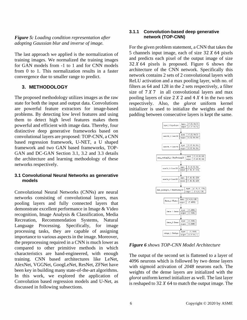
3.1.1 Convolution-based deep generative network (TOP-CNN)

For the given problem statement, a CNN that takes the

5 channels input image, each of size 32 𝑋 64 pixels

and predicts each pixel of the output image of size

32 𝑋 64 pixels is proposed. Figure 6 shows the

architecture of the CNN network. Specifically this

network contains 2 sets of 2 convolutional layers with

ReLU activation and a max pooling layer, with no. of

filters as 64 and 128 in the 2 sets respectively, a filter

size of 7 𝑋 7 in all convolutional layers and max

pooling layers of size 2 𝑋 2 and 4 𝑋 4 in the two sets

respectively. Also, the glorot uniform kernel

initializer is used to initialize the weights and the

padding between consecutive layers is kept the same.

Figure 6 shows TOP-CNN Model Architecture

The output of the second set is flattened to a layer of

4096 neurons which is followed by two dense layers

with sigmoid activation of 2048 neurons each. The

weights of the dense layers are initialized with the

glorot uniform kernel initializer as well. The last layer

is reshaped to 32 𝑋 64 to match the output image. The


proposed CNN (calling TOP-CNN) has a total of

14,008,000 trainable parameters. The Adam

optimizer [10] with a default learning rate of 0.001,

momentum parameters β1 = 0.9, β2 = 0.9, epsilon

value of 1e-07 and Mean Squared Error (MSE) loss

function is used for training the CNN for 100 epochs

with a batch size of 256. Figure 7 shows the learning

curve of the trained CNN with a training loss of

0.0029 and testing loss of 0.0154 at the end of 100

epochs. Here the test dataset consists of 0.5% of the

entire dataset.

Figure 7 shows the learning curve of TOP-CNN

Model.

3.1.2 U-Shaped Auto-Encoder with Skips (U-Net)

The U-shaped neural network (U-Net) is built based

on convolutional network and down-sampling the

input data through encoding technique and up-

sampling the result through decoding technique. The

main difference is U-Net is symmetric and it applies

a concatenation operator to connect the down-

sampling and up-sampling path. Due to the features of

the structure, it can provide many feature mappings,

which is local information to global information in the

up-sampling path. Because of this architecture, the

size of input data is reduced but the core components

remain the same.

The input size of images is 32X64, through two

convolutional layers, saving output of Conv2D. Then

passing to Max Pooling layers to reduce the size of the

feature map that it has fewer parameters to compute

in the network, which is down-sampling. After that,

when it goes through convolutional operation again,

the filter in the layer will be able to see larger context

which means going to a deeper network and saving

output. The process is repeated. When the network

reaches the final Conv2D layer, it starts doing

transposed convolution to up-sampling the image

with learnable parameters, which through back

propagation to convert a low-resolution image to high

resolution image. The output of up-sampling

concatenates with the saved outputs from Conv2D

layer. After every concatenation, it has two

consecutive regular convolutions so that the model

can learn to assemble precise output. The architecture

is a symmetric U-shape (See Figure 8), which is called

U-Net. We implemented this model to test the

applicability on this problem.

he input size of images are 32X64, through two

convolutional layers, saving output of Conv2D. Then

passing to Max Pooling layers to reduce the size of the

feature map that it has fewer parameters to compute

in the network, which is down-sampling. After that,

when it goes through convolutional operation again,

the filter in the layer will be able to see larger context

which means going to a deeper network and saving

output. The process is repeated. When the network

reaches the final Conv2D layer, it starts doing

transposed convolution to up-sampling the image

with learnable parameters, which through back

propagation to convert a low-resolution image to high

resolution image. The output of up-sampling

concatenates with the saved outputs from Conv2D

layer. After every concatenation, it has two

consecutive regular convolutions so that the model

can learn to assemble precise output. The architecture

is a symmetric U-shape (See Figure 8), which is called

U-Net. We implemented this model to test the

applicability on this problem.


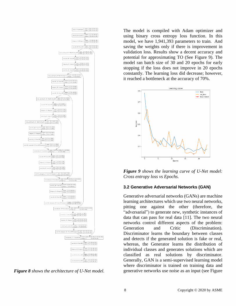
Figure 8 shows the architecture of U-Net model.

The model is compiled with Adam optimizer and

using binary cross entropy loss function. In this

model, we have 1,941,393 parameters to train. And

saving the weights only if there is improvement in

validation loss. Results show a decent accuracy and

potential for approximating TO (See Figure 9). The

model ran batch size of 30 and 20 epochs for early

stopping if the loss does not improve in 20 epochs

constantly. The learning loss did decrease; however,

it reached a bottleneck at the accuracy of 70%.

Figure 9 shows the learning curve of U-Net model:

Cross entropy loss vs Epochs.

3.2 Generative Adversarial Networks (GAN)

Generative adversarial networks (GANs) are machine

learning architectures which use two neural networks,

pitting one against the other (therefore, the

“adversarial”) to generate new, synthetic instances of

data that can pass for real data [11]. The two neural

networks control different aspects of the problem:

Generation and Critic (Discrimination).

Discriminator learns the boundary between classes

and detects if the generated solution is fake or real,

whereas, the Generator learns the distribution of

individual classes and generates solutions which are

classified as real solutions by discriminator.

Generally, GAN is a semi-supervised learning model

where discriminator is trained on training data and

generative networks use noise as an input (see Figure


5(a)). Additionally, discriminator operates like a

normal binary classifier that can classify images into

different categories and the generative model tries to

generate features as per the given class. Different

types of GAN are Vanilla GAN, Deep Convolutional

GANs (DCGANs), Conditional GANs (cGANs),

Laplacian Pyramid GAN (LAPGAN), StackGAN,

InfoGAN, Wasserstein GANs, Disco GANS, etc and

innovative GANs are developed everyday due to the

wide range of application.

For the given problem statement, we decided to

implement two Conditional GAN’s which aims at

generating images with optimized topology.

Conditional GAN’s are the GAN’s which uses a class

or label as input for both generator and discriminator

[12] (See Figure 10 (b)). This type of network can

consider the user’s desire of generating a solution to

an input problem. This type of network is suitable for

the project as we plan to generate solutions to a

diverse range of problems with varying geometric

constraints and boundary and loading conditions.

Particularly we implemented two different types of

conditional GAN: TOP-GAN and Conditional DC

GAN, as discussed in following subsections.

Figure 10 shows Different type of Conditional GAN

3.2.1 Novel generative adversarial network (TOP-GAN)

Considering diverse training data, we developed a

novel GAN architecture called TOP-GAN which

employs best model design heuristics from existing

networks in literature. Specifically, TOP-GAN uses

U-Net as a generator to generate solutions based on

input problems, defined as an image with five

channels (See Section 2, Figure 3). The input images

are normalized from -1 to 1; to make sure the mean is

zero. The architecture of U-Net is shown in Figure

11).

Figure 11 shows the U-Net Generator Model

U-Net is an autoencoder-type network with an

encoder and decoder that are related by skips (See

Figure 11). The proposed U-Net architecture initiates

with an input of 5 channels with resolution 32X64.


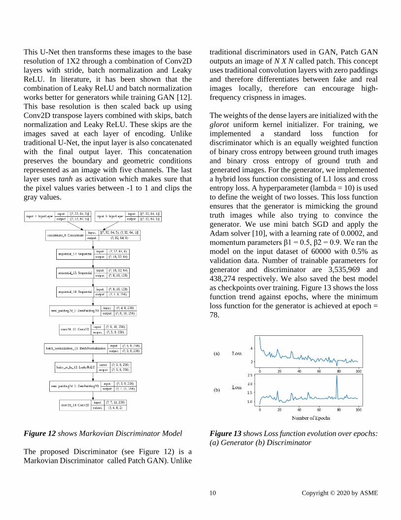
This U-Net then transforms these images to the base

resolution of 1X2 through a combination of Conv2D

layers with stride, batch normalization and Leaky

ReLU. In literature, it has been shown that the

combination of Leaky ReLU and batch normalization

works better for generators while training GAN [12].

This base resolution is then scaled back up using

Conv2D transpose layers combined with skips, batch

normalization and Leaky ReLU. These skips are the

images saved at each layer of encoding. Unlike

traditional U-Net, the input layer is also concatenated

with the final output layer. This concatenation

preserves the boundary and geometric conditions

represented as an image with five channels. The last

layer uses tanh as activation which makes sure that

the pixel values varies between -1 to 1 and clips the

gray values.

Figure 12 shows Markovian Discriminator Model

The proposed Discriminator (see Figure 12) is a

Markovian Discriminator called Patch GAN). Unlike

traditional discriminators used in GAN, Patch GAN

outputs an image of N X N called patch. This concept

uses traditional convolution layers with zero paddings

and therefore differentiates between fake and real

images locally, therefore can encourage high-

frequency crispness in images.

The weights of the dense layers are initialized with the

glorot uniform kernel initializer. For training, we

implemented a standard loss function for

discriminator which is an equally weighted function

of binary cross entropy between ground truth images

and binary cross entropy of ground truth and

generated images. For the generator, we implemented

a hybrid loss function consisting of L1 loss and cross

entropy loss. A hyperparameter (lambda = 10) is used

to define the weight of two losses. This loss function

ensures that the generator is mimicking the ground

truth images while also trying to convince the

generator. We use mini batch SGD and apply the

Adam solver [10], with a learning rate of 0.0002, and

momentum parameters β1 = 0.5, β2 = 0.9. We ran the

model on the input dataset of 60000 with 0.5% as

validation data. Number of trainable parameters for

generator and discriminator are 3,535,969 and

438,274 respectively. We also saved the best model

as checkpoints over training. Figure 13 shows the loss

function trend against epochs, where the minimum

loss function for the generator is achieved at epoch =

78.

Figure 13 shows Loss function evolution over epochs:

(a) Generator (b) Discriminator


3.2.2 Modified Deep Convolution based generative adversarial network (DC-GAN)

We implemented a DC-GAN model with a

regression-based deep convolutional neural network

as generator and a convolutional based classifier. This

type of generative models are also used in CWGAN

[7]. The input images to the generator have 5 channels

which are then transformed to one channel image and

is the output of the encoder. These newly generated

images and the training dataset are input to the

discriminator. The images are discriminated against

as fake or real. The architecture of the generator and

discriminator are shown in figure 14 and figure 15,

respectively.

Figure 14 shows Generator Model for GAN

The input image to the generator is of dimension

32x64 with 5 channels. This input images are then

transformed to 1X2 with 126 channels using a

combination of Conv2D layers, batch normalization

and leaky ReLU. Then the transformed image is

flattened into an array of size 512. This transformed

array is feeded into a couple of dense layers and then,

reshaped back into the output image size. Couple of

Conv2D transpose layers are also added. The last

layer has activation function tanh. Like TOP-GAN, a

hybrid loss function is implemented comprise of L1

and binary cross entropy loss. L1 loss acts as a

regularization parameter and therefore, avoids

sticking in the local minima. The total generator loss

is a weighted summation of both the losses. The

number of trainable parameters for generator are

3,336,549.

Figure 15 shows Discriminator Model for DCGAN


Unlike TOP-GAN, the discriminator is modified DC-

GAN is a convolutional based classifier, outputting a

single value describing the input image is fake (-1)

and real (+1). Two images are feeded into

discriminator: generated image from generator or the

target as the first image and the input image

describing the design problem as second image. These

two images are concatenated at first and then down

sampled by passing through convolution and then

dense layers to get the single output. The activation

function used for the final dense layer is sigmoid to

limit the range of values from -1 to 1. The loss

function used for the discriminator is a weighted cross

entropy function describing the conditional loss. We

scaled down the discriminator loss by 0.5, to reduce

the learning rate of discriminator. The trainable

parameters in the discriminator are 172,129. Adam

solver [10] is used for both generator as well as

discriminator. The learning rate used is 1e-4 for the

generator and 1e-6 for the discriminator. The

generator converges near 40 epochs.

Figure 16 shows the loss function evolution over

epochs: (a) Generator (b) Discriminator

4. RESULTS

To compare models, we evaluated the model on a

common dataset with 5000 data points. By having a

common dataset, it provides a base for an accurate

comparison. Since all the models do not follow

standard norms: common loss functions and accuracy

metrics, we decided to evaluate mean absolute error

(MAE or L1 loss) as a common metric for

comparison. Figure 17 shows the result outputted

from proposed four models and corresponding L1

loss.

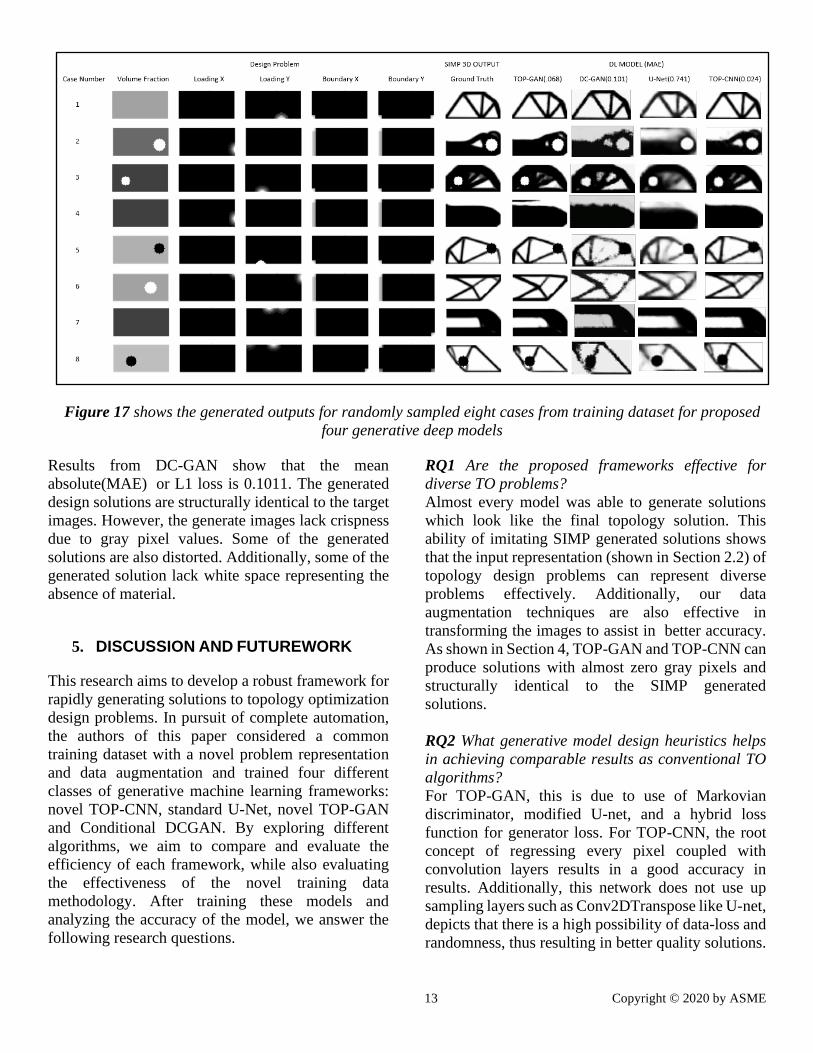
Results from TOP-CNN shows that the framework

can generate results close to the ground truth. The

network successfully learned the structural features,

location of boundary and loading conditions.

Moreover, the location and size of the active and

passive elements is very accurately captured.

Inappropriate grey pixels in the structure were

observed in a few cases. Thin members did not appear

as straight rigid members. Rather pixilation was

observed in the same. Results on the test dataset were

coherent with that of the training dataset. However, a

few cases of distorted circles for the active and

passive element were observed in the test dataset.

Results from UNET show it can generate some

topology of the input images which is basically like

the target output. However, it has some obvious

disadvantages of the solution. For example, in some

cases, the volume distribution of material under force

result is overlapping for complex boundary

conditions. On the other hand, the model can learn the

presence of active and passive elements from the

input images. Overall, the proposed U-Net can predict

somehow topology optimization results with 70%

accuracy and MAE = 0.741.

Results from TOP-GAN shows that the framework

can generate close-to-target solutions (validation

MAE = 0.06853). The generated solutions have fewer

gray pixels with no discrete volume. Additionally, the

model can predict structurally identical solutions to

SIMP 3D outputs. After evaluating the model on test

data, the results seem close to the output images. We

also observe a good mimicking behavior with features

regeneration; ability to understand loading, boundary,

geometric constraints, and volume fraction. We

observed a few cases where TOP-GAN failed to learn

smaller features and therefore, resulted in non-

plausible solutions (See Figure 17, case 4 TOP-GAN).

Comparatively, this model outperforms DC-

GAN and U-Net with a smaller number of trainable

parameters.


Results from DC-GAN show that the mean

absolute(MAE) or L1 loss is 0.1011. The generated

design solutions are structurally identical to the target

images. However, the generate images lack crispness

due to gray pixel values. Some of the generated

solutions are also distorted. Additionally, some of the

generated solution lack white space representing the

absence of material.

5. DISCUSSION AND FUTUREWORK

This research aims to develop a robust framework for

rapidly generating solutions to topology optimization

design problems. In pursuit of complete automation,

the authors of this paper considered a common

training dataset with a novel problem representation

and data augmentation and trained four different

classes of generative machine learning frameworks:

novel TOP-CNN, standard U-Net, novel TOP-GAN

and Conditional DCGAN. By exploring different

algorithms, we aim to compare and evaluate the

efficiency of each framework, while also evaluating

the effectiveness of the novel training data

methodology. After training these models and

analyzing the accuracy of the model, we answer the

following research questions.

RQ1 Are the proposed frameworks effective for

diverse TO problems?

Almost every model was able to generate solutions

which look like the final topology solution. This

ability of imitating SIMP generated solutions shows

that the input representation (shown in Section 2.2) of

topology design problems can represent diverse

problems effectively. Additionally, our data

augmentation techniques are also effective in

transforming the images to assist in better accuracy.

As shown in Section 4, TOP-GAN and TOP-CNN can

produce solutions with almost zero gray pixels and

structurally identical to the SIMP generated

solutions.

RQ2 What generative model design heuristics helps

in achieving comparable results as conventional TO

algorithms?

For TOP-GAN, this is due to use of Markovian

discriminator, modified U-net, and a hybrid loss

function for generator loss. For TOP-CNN, the root

concept of regressing every pixel coupled with

convolution layers results in a good accuracy in

results. Additionally, this network does not use up

sampling layers such as Conv2DTranspose like U-net,

depicts that there is a high possibility of data-loss and

randomness, thus resulting in better quality solutions.

Figure 17 shows the generated outputs for randomly sampled eight cases from training dataset for proposed

four generative deep models


Additionally, the use of tanh activation function at the

last layer of networks limits the production of gray

values.

This work shows a greater potential of deep learning

algorithms in rapid design generation for topology

optimization problems. By exploring and comparing

various algorithms, we confidently say that TOP-

CNN and TOP-GAN have the highest potential for the

rapid design generation. Further investigation is

necessary to improve accuracy and evaluate test cases

that were not present in training data. Additionally,

we see an exciting opportunity in combining

reinforcement learning algorithms with generative

algorithms for better accuracy and versatility. In

future, we would like to consider other boundary

conditions as well and evaluate if proposed

frameworks are able to generate solutions or not.

6. RESULTS

In this study, we aimed at developing and comparing

machine learning frameworks for generating rapid

solutions to topology optimization design problems.

Specifically, we developed a novel problem

representation using a 5 channels image, consisting of

boundary, and loading conditions, volume fraction

needed and design space information. Additionally,

this representation also incorporates a variety of

loading conditions using a novel force representation

using intensity of pixels. With this robust

representation of design problems and generated TO

results using SIMP, we trained four different

generative models to evaluate the effectiveness and

learn methodological design heuristics to obtain

comparable rapid design solutions. The four

generative models developed are CNN regression

(TOP-CNN), U-Net , GAN with U-Net as generator

(TOP-GAN) and GAN with CNN regressor as

generator (DCGAN). These generative models are

trained on a randomly selected dataset of 60000 with

varying validation splits for each model. The training

data includes a diverse range of problems with

varying active and passive elements, volume fraction,

loading and boundary conditions. In addition, we also

implemented data augmentation techniques such as

gaussian blur, inverting images, and normalization to

assist generative models to learn problems efficiently.

All the models were trained in batches to balance-out

computational resources by reducing memory usage.

Results show that all the models were able to learn the

TO problems, but with varying accuracy and

versatility. Our findings indicate that TOP-CNN and

TOP-GAN outperforms other networks and can

imitate the computationally expensive SIMP method.

We also observed an additional benefit of using

Markovian discriminator for providing a localized

feedback in TOP-GAN. For TOP-CNN, the idea of

predicting every pixel value of final output, the use of

tanh activation functions and the simplicity of the

model.

REFERENCES

[1] R. Jin, W. Chen, and T. W. Simpson,

“Comparative studies of metamodelling

techniques under multiple modelling criteria,”

no. 1998, pp. 1–13, 2001.

[2] T. Zegard and G. H. Paulino, “Bridging

topology optimization and additive

manufacturing,” Struct. Multidiscip. Optim.,

vol. 53, no. 1, pp. 175–192, 2016, doi:

10.1007/s00158-015-1274-4.

[3] J. Liu et al., “Current and future trends in

topology optimization for additive

manufacturing,” Struct. Multidiscip. Optim.,

vol. 57, no. 6, pp. 2457–2483, 2018, doi:

10.1007/s00158-018-1994-3.

[4] J. Liu, “An Efficient and High-Resolution

Topology Optimization Method Based on

Convolutional Neural Networks,” no. October,

2019, doi: 10.20944/preprints201910.0137.v1.

[5] S. Banga, H. Gehani, S. Bhilare, S. Patel, and

L. Kara, “3D Topology Optimization using

Convolutional Neural Networks,” 2018.

[6] Y. Zhang, A. Chen, B. Peng, X. Zhou, and D.

Wang, “A deep Convolutional Neural Network

for topology optimization with strong


generalization ability,” no. 2017, 2019.

[7] S. Rawat and M.-H. H. Shen, “A Novel

Topology Optimization Approach using

Conditional Deep Learning,” 2019.

[8] O. M. Querin, M. Victoria, C. Alonso, R.

Ansola, and P. Martí, “Hands-On Applications

of Structural Optimization,” in Topology

Design Methods for Structural Optimization,

Elsevier Ltd, Ed. Elsevier Ltd, 2017, pp. 71–

91.

[9] E. Andreassen, A. Clausen, M. Schevenels, B.

S. Lazarov, and O. Sigmund, “Efficient

topology optimization in MATLAB using 88

lines of code,” Struct. Multidiscip. Optim., vol.

43, no. 1, pp. 1–16, 2011, doi: 10.1007/s00158-

010-0594-7.

[10] D. P. Kingma and J. L. Ba, “Adam: A method

for stochastic optimization,” 3rd Int. Conf.

Learn. Represent. ICLR 2015 - Conf. Track

Proc., pp. 1–15, 2015.

[11] I. Goodfellow, “NIPS 2016 Tutorial:

Generative Adversarial Networks,” 2016.

[12] P. Isola, J. Y. Zhu, T. Zhou, and A. A. Efros,

“Image-to-image translation with conditional

adversarial networks,” Proc. - 30th IEEE Conf.

Comput. Vis. Pattern Recognition, CVPR

2017, vol. 2017-Janua, pp. 5967–5976, 2017,

doi: 10.1109/CVPR.2017.632.

Documents

A SYSTEMATIC STUDY OF DEEP GENERATIVE MODELS FOR …