Embed Size (px)
Citation preview

A Survey of Methods for
Data Inclusion in System Dynamics Models:
Methods, Tools and Applications
James Houghton, Michael Siegel, Anton Wirsch,
Allen Moulton, Stuart Madnick, Daniel Goldsmith
Working Paper CISL# 2014-03
May 2014
Composite Information Systems Laboratory (CISL)
Sloan School of Management, Room E62-422
Massachusetts Institute of Technology
Cambridge, MA 02142
1
A Survey of Methods for Data Inclusion in System Dynamics Models
Methods, Tools and Applications
James Houghton, Michael Siegel, Anton Wirsch, Allen Moulton, Stuart Madnick, Daniel
Goldsmith
In 1980, Jay Forrester 1 enumerated three types of data needed to develop the structure and
decision rules in models: numerical, written and mental data, in increasing order of
importance. While this prioritization is appropriate, it is numerical data that has
experienced the most development in the 25 years since Forester made his enumeration. In
this paper, we’ll focus on how numerical data can be incorporated into models when
written and mental data are known, and survey the techniques for doing so.
Motivation and Purpose
Numerical data is experiencing a renaissance because 1) traditional data such as census and
economic surveys are more readily accessible 2) new sensors are measuring things that
have never been measured before, and 3) previously 'unstructured' data - such as raw text,
audio, images, and videos - is becoming more amenable to quantification2.
Because of this explosion and the popular buzz surrounding ‘Big Data’, clients expect to see
strong incorporation of data methods into dynamic models, and it is imperative that System
Dynamics Modelers are fully versed in the techniques for doing so.
The SD literature contains surveys (Peterson 19763 and Eberlein 19854) that explain
methods for including data in system dynamics modeling, but techniques have continued to
develop. This paper attempts to bring these surveys up to date, and serve as a menu of modern
techniques.
Structure
The paper is structured to follow the modeling process laid out by John Sterman in
'Business Dynamics'5: 1) Problem Articulation and Boundary Selection, 2) Formulation of a
Dynamic Hypothesis, 3) Formulation of a Simulation Model, 4) Testing, 5) Policy Design and
Evaluation.
Within each major step we discuss specific modeling tasks and relevant data techniques,
and give a brief overview of the mechanics of that technique. We refer the reader to seminal
works and good tutorials for further learning. Where appropriate we list some of the major
software packages that support each technique. We show how the technique can be used
specifically in the modeling task, with examples drawn from System Dynamics and related
literature.

2
Scope
This is clearly not an exhaustive list of data techniques that could be applied to System
Dynamics. Instead, we survey the techniques that have precedent in the SD literature, and
draw support from outside traditions.
We choose only to touch on the parts of the model building process that show clear promise
of benefitting from numerical data. We choose not to investigate methods of data collection
or elicitation, which are covered elsewhere6.
1 Problem Articulation and Boundary Selection The first and most important model-building step is to clearly identify the purpose for a
model and the problem that it hopes to solve. This step requires investigation of the
dynamic behavior of the system and its problem symptoms, and determination of the
appropriate scope and resolution of the model. Randers explains this step in the classic
'Guidelines for Model Conceptualization'7; Mashayekhi and Ghili8 discuss problem definition as
an inherently iterative process. From this section we omit qualitative tasks: phrasing the
research question, description of problem behavior, and choice of model structure
boundary, in order to focus on tasks with a strong data dependency.
1.1 Identify Reference Modes
A modeler should be able to identify the symptoms of problem behavior in the time-series
data that the problem system generates. The process of identifying these reference modes is
described well by Saeed9 and VanderWerf10.
Finding reference modes within time-series data is not always straightforward, and may
require the modeler to look at the data in a variety of ways before the behavior becomes
clear.
1.1.1 Exploratory Data Analysis and Data Visualization
Exploratory Data Analysis refers to visualization and statistical summary techniques that
are designed to give the modeler an intuitive understanding of the nature of the data.
Description
Visualization methods generally show how a parameter of interest varies according to an
independent attribute (time, geography, property, or relationship). Summary statistics can
investigate the relationship of data with itself, by looking at averages, variances, and
correlations.
Among others, Tukey11 promoted Exploratory Data Analysis for development of intuition
about data; in the years that followed, data visualization and summary statistics have
become an integral part of introductory statistics courses, and are an ongoing area of
research. Tufte12 provides the quintessential resource for visualization of quantitative
information, and Yau13 gives an introduction to modern techniques and tools. Keim14
discusses visualization as a form of Data Mining.

3
The vast majority of data or numerical analysis software suites provide some form of
summary statistic and data visualization capability: Python(NumPy15, Matplotlib16,
Bokeh17), R(native), Javascript(D318), Matlab19(native), Gnuplot20, etc.
Application to Reference Mode Identification
To identify behavior modes, the modeler needs to have a good understanding of the
dynamic behavior of the system. Exploratory Data Analysis in the form of visualization and
simple summary statistics allows the modeler to form that intuition by presenting
numerical data in human-digestible formats. These formats allow the modeler’s eyes to look
past noise to see the variety of growth, decay, or oscillatory modes that constitute the
behavior of interest. Khan, McLucas and Linard21 use a variety of visual and aggregation
methods to develop reference modes for the salinity of the Murray Darling basin.
1.1.2 Frequency Spectrum Analysis
Frequency Spectrum Analysis allows the modeler to see the strength of each of the
oscillatory modes in her sample data.
Description
It is not uncommon to think about time-series data as being
composed of a number of oscillations at different frequencies
superimposed on one another. Fourier transforms are used to
estimate the relative contribution of each of these oscillatory
modes to the measurements. Fourier transforms come out of the
signal processing community, with a seminal paper by Cooley and
Tukey22, and a good overview of the method by Duhamel23.
Software packages that support Fast Fourier Transforms and
Frequency Spectrum Analysis include Python (Numpy.fft24), R
(Stats.spectrum25), Matlab26 (fft), and Excel (Analysis Toolpack)
Application to Reference Mode Identification
Frequency Spectrum Analysis can reveal the dominant modes of
oscillation, and help the modeler identify the frequency band that
captures the behavior of interest. Arango and Moxnes27
demonstrate the use of Spectral Analysis to identify cyclical behavior in energy markets, as
can be seen in Figure 1.
1.1.3 Phase Portraits
A phase portrait factors out the time component of a model to show how a pair of system
components vary with respect to one another. The shape of the phase portrait curves can
show if one variable is driving another, or if they oscillate in-phase or opposed to one
another. A phase portrait can show if oscillations are being damped or becoming unstable, if
the oscillations follow a standard pattern, or if the system is exhibiting chaotic behavior.
Figure 1: Market Price History and Spectral Density in Arango and Moxnes27, showing two major
oscillatory modes.

4
Description
A phase portrait is a set of curves whose x coordinate is
described by the values of one variable of interest, and the
y coordinate described by another. A phase portrait may
show the direction of the flow in this space when the
system is initialized with a variety of values for each
parameter.
Phase plane analysis is frequently used in the Control
Theory and Complexity Theory traditions. A number of
texts provide introduction to phase plane analysis. See
Chapter 2 in Enns and McGuire28, Chapter 2 in Tien29, and
Tseng30. Most plotting tools can create a phase portrait,
although some provide more established mechanisms for
doing so, including Python (PyDSTool31), and Matlab26
(pplane).
Application to Reference Mode Identification
Phase portraits can be useful tools in determining behavioral modes and dynamic causal
influence. When phase plots show cyclic behavior the modeler can expect to see second
order structure driving the model. When the motion of stocks is well correlated, she should
look for a behavior that drives both, and so forth. Guneralp32 demonstrates the use of phase
portraits to understand the dynamic behavior of a variety of simple system structures, as
can be seen in Figure 2.
1.2 Infer Appropriate Aggregation Levels
System dynamics depends on the ability to aggregate individual actors or elements into
groups whose behavior can be modeled as a unit. These groups may be based upon age,
location, or other characteristics that define the group and its expected behavior. Rahn33
describes how the process of aggregation can make stochastic behavior into analytically
tractable flows, and takes a good look at this essential component of System Dynamics
modeling.
In many cases there will be a natural set of choices for levels of aggregation, or a standard
for doing so. For instance, students may be aggregated by grade, or into Elementary, Middle,
or High School. When such a clear-cut distinction is not available, clustering algorithms can
be used on the dataset to determine groups.
1.2.1 Machine Learning Clustering Algorithms
Description
Clustering algorithms work to identify sets of data-points in which the difference in
attributes between members of each group is minimized, and the difference between
groups is maximized. There are a variety of clustering algorithms that produce different
Figure 2: Phase plane demonstration of second order system in Guneralp32.

5
types of clusters. Clustering Algorithms come out of the Artificial Intelligence community,
and a survey of these algorithms is provided by Xu and Wunsch34.
Software packages that provide clustering algorithms include Python (Scikit-Learn35), R
(various packages), Matlab (Statistics Toolbox)
Application to Data Aggregation
In situations where intuitive or standardized methods of aggregation are infeasible, the
modeler may choose to use a machine learning algorithm to identify cohorts based upon
their shared attributes. Onsel, Onsel, and Yucel36; and Pruyt, Kwakkel, and Hamarat37
discuss clustering of behavior modes, although direct clustering for aggregation remains to
be demonstrated in SD literature.
2 Formulation of Dynamic Hypothesis In the second stage of model building, the modeler begins to determine the structure of the
model in a largely qualitative way. Inferring the overall structure of a model based upon
data is challenging, although there have been some attempts to do so. Data methods can be
more helpful in an iterative modeling process where the structure of a new model may be
based upon previous similar models, and the inference task is to infer which of a set of
previous models best represents the current data. We omit here causal mapping of the
system as this is the step in which the modeler begins to add written and mental data to the
model, and as such is less of a numerical task. We also omit the creative and intuitive task of
actual hypothesis generation.
2.1 Model Selection
In some cases there may be disagreement about the general structure of the system, as
different parties have different mental models of the way the system works. If simple
versions of these mental models are specific, data methods can be used to determine the
relative likelihood that each model structure could be responsible for creating the observed
data. The relative likelihoods of the model without respect to parameters are calculated as
'Bayes Factors'.
2.1.1 Markov Chain Monte Carlo
Markov Chain Monte Carlo (MCMC) can be used to infer the distributions of input
parameters to a model when the output behavior of the system is known through
measurement. In model selection, MCMC assumes the choice of model to be the parameter
of interest.
Description
MCMC chooses a random set of parameters from 'prior' input distributions, executes a
system model (which must have a stochastic component), and then calculates the likelihood
of the observed data given the run of the model and the chosen input parameters. The
algorithm uses this probability to decide whether to include the chosen input parameters in
a posterior distribution. Repeating this process on the order of tens or hundreds of

6
thousands of times, distributions for the input parameters can be summarized using
histograms or other density estimation methods.
Markov Chain Monte Carlo was developed to support nuclear engineering; and the primary
algorithms used in MCMC were developed by Metropolis38, Hastings39, and Geman and
Geman40. Andrieu, Freitas, Doucet and Jordan41; and Brooks42 give good introductions to use
of the technique. Software packages that provide MCMC algorithms include
Python(PyMC43), BUGS44, winBUGS, R(MCMCpack), Vensim.
Application to Model Selection
A modeler can use Markov Chain Monte Carlo to help choose between multiple competing
models. To do so she establishes a categorical variable that can take values corresponding
to each of the candidate models. In each MCMC run, a value (and thus a model) is selected
and the likelihood of the data given that model computed. After MCMC convergence, the
relative likelihood of each model is proportional to the number of times its categorical
variable value was selected.
Andrieu, Djuric and Doucet45 expand on their introduction to MCMC with a description of
how the method can be used to choose between models.
2.1.2 Bayes Factors
Bayes Factors serve as a relative likelihood of the validity of two models. While they won't
tell the modeler that a particular model is correct, they will tell her if one model is a better
representation of the measured data than another model.
Description
The Bayes Factor lets a modeler abstract the model from its parameters by calculating the
likelihood ratio of the two models under any set of parameters that each model takes as
valid. This takes the form of an integral of the likelihood over the parameter space. As this is
often a large multidimensional integral, the modeler can use a sampling technique such as
Markov Chain Monte Carlo to approximate its value.
Bayes Factors come from the statistics tradition and were first articulated by Jeffreys46. Kass
and Raftery47 give an overview of the technique in its modern form. Software packages that
specifically facilitate the calculation of Bayes Factors include Python (PyMC43), and
R(BayesFactor).
Application to Model Selection
Bayes Factors give weight to the preference one model should receive over another, and
thus give a measure of confidence in deciding to reject one model in favor of its competitor.
Alternately, the Bayes Factor may tell the modeler that there is no clear preference for one
model over the other, and that some form of averaging, or a new model altogether, would be
the preferred solution.
Raftery48 demonstrates the use of Bayes Factors for model selection on social research.
Opportunities exist for demonstrations of this technique in the SD literature.
7
3 Formulation of Simulation Model Data methods can be extremely helpful in completing dynamic models whose structures
have already been identified. The modeler can use these methods to help select equations to
represent the relationships between system components, identify values for model
parameters and initial conditions, and prepare exogenous inputs. Here we omit partial
models and other methods of slicing the model before inference, as they are well
established within System Dynamics and are not themselves data methods.
3.1 Identify Equations to Represent Relationships Between Variables
When a stock and flow structure has been constructed, the next step is to implement the
equations that govern each relationship. In some situations the modeler can work from first
principles, or infer scaling laws and nonlinearities from intuition. In other situations, she
may have little understanding of how variables relate to one another and must infer the
nature of the relationship from data.
3.1.1 Structural Equation Modeling
Structural Equation Modeling (SEM) attempts to infer relationships between a latent or
unobserved variable and a number of observed variables. These latent variables may be
estimators for a 'soft' quantity (such as 'morale') which itself may be further used in the
model.
Description
SEM tries to fit the covariance matrix of a predictive model to the covariance of the
observed parameters. Wright49 provided the seminal paper on Structural Equation
Modeling. Ullman50 gives a tutorial of the basics of SEM, using a substance abuse model as a
motivating example. A number of books give more detailed introductions, consider Kline51,
or Bollen52.
SEM is well represented in the psychology and econometrics traditions. Several statistical
suites have developed packages for structural equation modeling, including R(SEM,
OpenMX), and SPSS(Amos).
Application to Equation Identification
SEM is applied to System Dynamics modeling as a method for including 'soft' variables into
feedback models, identifying the relationship between the unobservable variable and
additional observable characteristics.
Medina-Borja and Pasupathy53 demonstrate the use of SEM in the context of a customer
satisfaction and branch expansion model for a bank. Roy and Mohapatra54 use SEM in a
model of research and development laboratories.
3.2 Identify Influential Parameters
In parameterizing the model, it’s likely that some parameters will have a strong influence on
the outcome of the model, and others less so. If a modeler can identify these, she can
prioritize the effort given to measuring each parameter value.

8
3.2.1 Sensitivity Analysis
Sensitivity analysis (also called Experimental Uncertainty Analysis or Propagation of Error)
is a method for determining the impact of small changes of a system input parameter upon
the computed output of the system.
Description
Sensitivity analysis uses numerical means such as Monte Carlo Analysis (see Section 4.2.1)
to propagate errors or uncertainties in model parameters through to the model output. It is
often performed one parameter at a time, and the relative magnitude of change between the
input and output compared with that of other parameters. It can also be performed for
multiple parameters simultaneously to determine the nonlinear interactions between
parameters on the output.
Helton, Johnson, Sallaberry and Storlie55 give an overview of sampling-based methods for
sensitivity analsysis in which they step through the various stages of the process: defining
input distributions, designing samples of those distributions and executing the model, and
reviewing the outcome; with a motivating example from industrial engineering.
Basic sensitivity analysis can be performed by any software capable of performing Monte
Carlo Analysis, although a few packages have been developed to implement more advanced
Sensitivity Analysis algorithms: Python(SALib56), R(Sensitivity), Matlab(Control System
Toolbox).
Application to Influential Parameter Identification
When sensitivity analyses are used in the model-building stage, the modeler is interested in
finding the parameters with the greatest need for precision - these being the parameters for
which a small error can lead the model to different conclusions. For each parameter, the
modeler can calculate how tight the error bounds must be such that its relative contribution
to the model uncertainty matches that of the other parameters.
Sharp57 discusses methods of sensitivity analysis specifically in the System Dynamics
setting. Powell, Fair, LeClaire and Moore58 use sensitivity analysis to identify crucial
parameters in an infectious disease model, and Hekimoglu and Barlas59 apply the method to
several business management problems.
3.2.2 Statistical Screening
Statistical Screening is a method of performing sensitivity analysis in system models that
are computationally expensive, and it is infeasible to take a large number of samples.
Description
Screening looks at the correlation between variables and output values, instead of looking
at the standard deviation of a number of samples when input values are varied. Welch et
al60 write an influential paper describing the process of statistical screening.
9
Application to Influential Parameter Identification
Statistical screening is important to the field of System Dynamics for its ability to identify
and prioritize data collection and parameter estimation tasks. Ford and Flynn61
demonstrate the use of statistical screening to identify influential parameters in SD models,
with examples of sales vs. company growth, and the World3 model. Taylor, Ford, and Ford62
demonstrate screening for application to a diffusion model and a rework model.
3.3 Summarize Measureable Parameters
In the ideal case, parameters of the model correspond to unique, observable characteristics
of the real system. The task of preparing measurements of this characteristic for inclusion in
System Dynamics models involves summarizing disaggregate sample data into single values
or distributions that represent the true distribution of the concept in the system. Graham63
gives an overview of this process, along with some traditional techniques for doing so.
3.3.1 Bootstrap Resampling
Resampling with bootstrap allows the modeler to estimate
the error in the parameters of a probability distribution,
based upon a finite number of observations of that
distribution. (Note that statistical bootstrapping is distinct
from bootstrap aggregating in machine learning.)
Description
Bootstrapping works by taking a subset of the sample data,
and computing the parameter of interest (mean, median,
etc.) for that subset. Repeating this process a large number
of times can give confidence bounds for the likely values of
the parameter in the sample data set, which are
comparable to the bounds on the true population.
The bootstrap method comes from the statistics tradition,
and was first introduced by Efron64; Henderson65, and
Diaconis and Efron66 provide tutorials and perspective on
the method and its variants. A variety of software packages facilitate statistical
bootstrapping, including Python (Scikit-Bootstrap67), R (Boot68), and Matlab (Statistics
Toolbox).
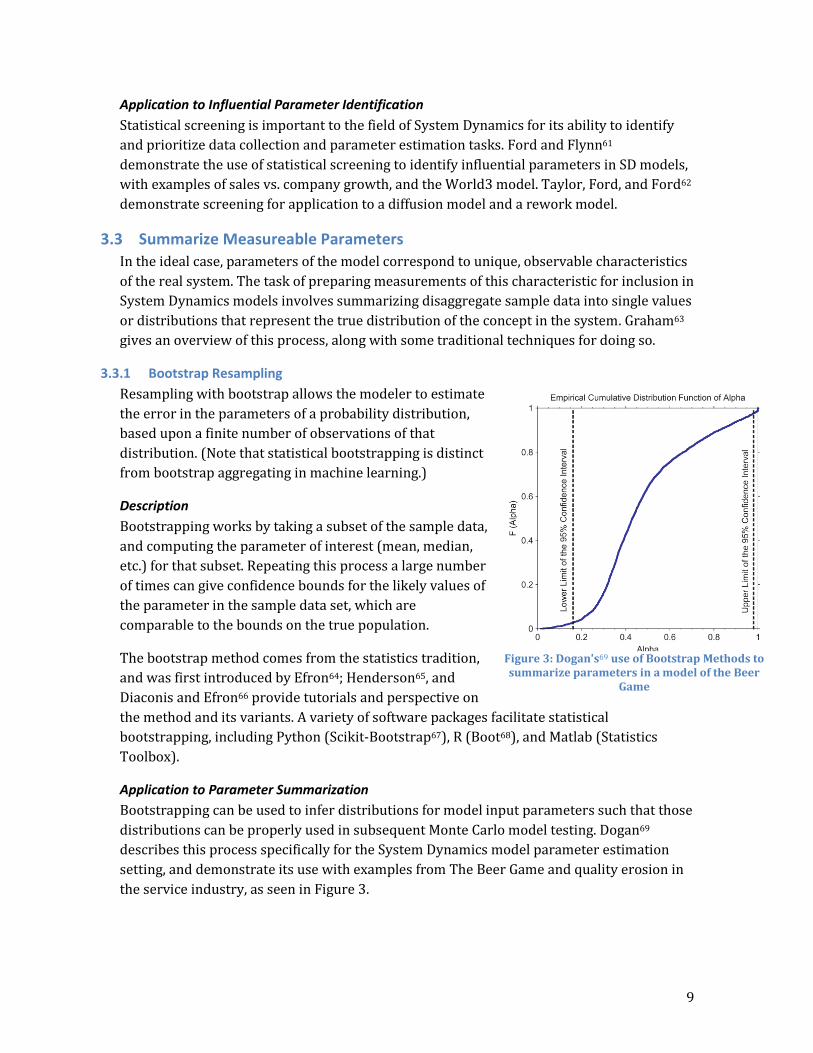
Application to Parameter Summarization
Bootstrapping can be used to infer distributions for model input parameters such that those
distributions can be properly used in subsequent Monte Carlo model testing. Dogan69
describes this process specifically for the System Dynamics model parameter estimation
setting, and demonstrate its use with examples from The Beer Game and quality erosion in
the service industry, as seen in Figure 3.
Figure 3: Dogan's69 use of Bootstrap Methods to summarize parameters in a model of the Beer
Game
10
3.3.2 Markov Chain Monte Carlo
For a description of Markov Chain Monte Carlo, please see section 2.1.1.
Application to Parameter Summarization
Markov Chain Monte Carlo can be used to estimate hyperparameters (such as mean and
standard deviation) for a distribution representing a SD model parameter. In such a case,
MCMC considers the data to be the product of a statistical model that takes the
hyperparameters to specify an analytical distribution, and calculates the likelihood of the
observed data. The MCMC algorithm then can be used to generate confidence intervals for
the hyperparameters, which can be used as input to the simulation model.
3.4 Infer Unmeasureable Parameters
There are many cases in which parameter values cannot be directly measured, but based
upon the model and its inputs and outputs, the modeler may be able to infer what the
parameter values would need to be for the system model and the data to make sense
together. She can perform this inference on either partial or full models, depending on the
data that is available, using a variety of numerical techniques to yield either single values or
distributions.
3.4.1 Regression
The concept of regression includes a variety of methods (Ordinary Least Squares,
Orthogonal Distance, Ridge, etc.) for identifying the single best set of parameter values for a
model, where 'best' is defined by some objective function, such as having the minimum
square error between model predictions and system measurements.
Description
Most regression methods perform an optimization (see section 5.1.1) over the parameter
space to minimize the difference between a prediction and system measurements. When
applied to time-series data, regression is most effective for non-oscillatory behavior modes.
A variety of resources for learning regression methods exist; consider Ryan70 or Vinod71.
The vast majority of statistical packages and System Dynamics modeling software give some
form of regression capability: Python (Scipy, Statsmodels72, Scikit-Learn), R(native), Matlab
(Statistics Toolbox), Vensim, AnyLogic (Model Calibration), etc.
Application to Model Parameter Inference
Multiple regression is a common method for inferring values for unknown parameters in
System Dynamics models. Higuchi73 discusses parameter estimation using regression with
an inventory model demonstration. Mayerthaler, Haller, and Emberger74 use regression to
parameterize a land use and transportation model.

11
3.4.2 Markov Chain Monte Carlo
For a description of MCMC, see Section 2.1.1.
Application to Model Parameter Inference
MCMC can be used to estimate a distribution for unknown
model parameter values if the output of the simulation
model is specified to represent the parameters of a
statistical distribution. In this case, parameters can be
sampled by the MCMC algorithm and the likelihood of data
given the sample parameters computed. The MCMC
algorithm traverses the parameter space, sampling from a
distribution representing the likelihood that each
parameter takes on a certain value. Osgood75 describes the use of Markov Chain Monte
Carlo for SD model parameterization.
3.4.3 Kalman Filtering
Kalman filtering gives an efficient method for calculating the unknown state of a system
given a set of noisy measurements.
Description
At each time-step, a Kalman Filter uses a System Dynamics model to predict the current
state of the system based upon its estimate of the previous state. It then combines its
prediction with a measurement of the state (or components of the state) based upon its
relative confidence in each.
Kalman filters were developed in support of the Apollo program, and come from an
Aerospace and Control Theory background. Kalman's original paper76 lays out the basics of
his filter, and Du Plessis77 gives a very readable introduction in 'The Poor Man's Explanation
of Kalman Filtering', only a few years later. Awasthi and Raj78 give a modern survey of the
filter's modern variants.
Kalman filters are available within a number of numeric tools, including Python
(Pykalman79), Matlab(Simulink, DSP Toolbox), R(several, compared by Tussel80), Vensim
and others.
Application to Model Parameter Inference
In a parameter estimation setting, parameters can be considered as unchanging states for
the Kalman Filter to infer. Examples of Kalman Filters applied to System Dynamics include
Ryzhenkov's parameterization of an economic long wave model81, and Shiryaev, Golovin
and Smolin's model of a one-commodity firm82.
Figure 4: Inference of Distributions with MCMC in Andrieu, Freitas, and Doucet41.

12
3.5 Surrogate a Function
In some cases, two variables exhibit a well-defined relationship, but the form of that
relationship is not well described by any simple functions. If these parts of the system are
not the subjects of interest, the modeler may choose to surrogate the relationship with
some form of piecewise model, or machine learning predictor.
3.5.1 Table Functions or Lookup Tables
Table functions give the modeler the ability to approximate a nonlinear relationship
between one or more independent variables and an output variable.
Description
When an analytic representation of the relationship is complex or unavailable, the modeler
constructs a table function using a set of points from that function, and these are
interpolated between to find output values.
Lookup tables have been in use long before the advent of computers, and had previously
been compiled to make trigonometric or logarithmic calculations simpler. Many software
packages provide the basic data storage and interpolation function necessary to implement
a lookup table, including Python(Scipy, Pandas83), R(Stats), matlab(native), Vensim,
Anylogic.
Application to Surrogating Functions
When a relationship between variables is unknown or complex, a lookup table provides an
intuitive way to include information about the relationship in a model. Franco84 presents a
thorough introduction to table functions as they have historically been used in SD modeling.
3.5.2 Neural Networks
Neural Networks have the ability to encode multidimensional nonlinear relationships based
directly upon training data, and to approximate a response to novel input that is consistent
with the nonlinear relationships it encodes.
Description
Neural networks use training data to establish the relative weights of a set of links between
neural nodes, these links encoding the relationships present in training data. Test data
forms the inputs to these models, and their interaction with the established links provides
the output.
Neural networks are a product of the Machine Learning community. McCulloch and Pitts85
developed the first concepts of Neural Networks well before they were implemented on
computer. Holena, Linke, Rodemerck, and Bajer86 use neural networks directly for
surrogating functions based upon data. Software capable of encoding neural networks
includes, Matlab(NN Toolbox), Python(NeuroLab87, PyBrain88), and a number of standalone
packages.
13
Application to Surrogating Functions
System Dynamicists can use neural networks in place of table functions, especially in
situations with complex, multidimensional relationships that must be estimated from data.
Alborzi89 demonstrates the use of a neural network to approximate a function, using the
example of gravitational attraction between two bodies.
4 Testing After the model is built, the next task is to build confidence in the model's ability to
represent the real system. Here the modeler can use data for its ability to disprove the
model, show where its weaknesses are, and determine how she can improve it. In each case
the modeler is looking at the model's ability to predict the data in a given set of conditions,
and to test the model's robustness to different types of errors. Forrester and Senge90 give a
definitive guide to System Dynamics model testing. Barlas91 elaborates with a procedure for
conducting various forms of model testing.
In this section we omit qualitative tests, such as tests for boundary adequacy, and
dimensional consistency; numerical tests with little reliance on data (beyond model
calibration): test of conservation laws, extreme conditions, loop knockout, and surprise
behavior tests. These omissions help us focus on the tests with strong data reliance.
4.1 Compare Point Predictions with Numerical Data
The most logical quantitative test of a predictive model is its ability to make predictions.
When a model is calibrated with best-fit parameter values, it is only able to make point
predictions, which are unlikely to follow the true behavior of the system exactly. A modeler
can look at the difference between the model prediction and the observed behavior in both
the time and frequency domain for various parts of the model and various sections of the
data.
4.1.1 Summary Statistics
Summary statistics aggregate the difference between a model point prediction and the
observed value, according to some weighting function. These can be decomposed into
components due to bias, variance, and covariance.
Description
Summary statistics include variants on Mean Square Error, the Coefficient of Determination,
Theil's U statistics, and others. Sterman92 describes the appropriate use of summary statistics
for System Dynamics models. Oliva93 shows how these metrics are calculated using Vensim.
The majority of statistical packages are capable of calculating basic summary statistics:
Python(Scikit-Learn, Statsmodels), R(Metrics), Vensim.
Application to Point Prediction Assessment
Summary statistics are used to estimate the goodness of fit of a model to historical data.
System Dynamics models are often interested not in the magnitude of the total error, but in

14
the way that error is composed. By using a variety of summary statistics a modeler can
determine if the error in her models is relevant to the purpose of the model. As an example,
Stephan94 uses summary statistics to build confidence in models of software development.
4.1.2 Cross Validation
Cross validation (or out-of-sample testing) works to improve confidence that the model
represents the underlying behavior of the system, and that correspondence between the
model and the observed data is not merely a result of over-fitting the model to the data.
Description
Cross validation works by breaking a dataset into 'training' and 'testing' components. The
training set is used to parameterize the model, and the testing set is used to measure the
ability of the model to make predictions. If possible, a modeler may choose to partition the
data in a variety of ways and repeat the analysis.
When the system is time-dependent (as is usually the case with feedback models) and data
is not significantly in excess of the relevant period of the system, there is a limited range of
ways that the data can be meaningfully partitioned.
Cross validation comes from the statistics tradition. Picard and Cook95 give a good overview
of the use of cross validation to combat over-fitting in regression models. Software that
facilitates cross validation includes Python (Scikit-Learn), R (A variety of packages
summarized by Starkweather96), Matlab(Statistics Toolbox) and others.
Application to Prediction Assessment
Cross validation in system dynamics can be challenging, as the complex time-dependent
nature of the systems in question increases the difficulty of partitioning data into
independent subsets. Randers97 demonstrates out-of-sample testing in the qualitative
comparison of predicted and measured wood pulp inventory and price.
4.1.3 Family Member Tests
Family Member Tests are a special form of cross-validation or out-of-sample testing, in
which the modeler uses the model structure to predict the behavior of a structurally parallel
but physically separate system. As with Cross Validation, Family Member Tests work to
verify that the model fit is due to the structure of the system model, and not to a lucky guess
of parameters.
Description
If appropriate family member systems are available, a modeler may choose to reoptimize
the model based upon data from the family-member system in order to support the fidelity
of the model structure and equations; or use the original parameter values to support the
full data and modeling process. The modeler can then apply either point-wise or statistical
measures to evaluate the model's predictive ability.
Family Member Tests are described by Forrester and Senge90, and well elaborated by
Sterman5(21.4.9).

15
Application to Prediction Assessment
System dynamics is principally concerned with identifying the structure of a system, and
structural similarities between systems. These similarities allow a model developed in the
context of one system to be applied to another, structurally similar system with few
changes. Teekasap98 tests a model of the economy of Thailand by evaluating its ability to fit
data for the structurally similar Malaysian economy.
4.1.4 Frequency Spectrum Analysis
For a description of the method, see section 1.1.2
Application to Point Prediction Assessment
In systems with oscillation and noise, small changes in system parameters can lead to large
deviation between model prediction and system observation after only a few periods.
Spectral analysis, however, can reveal similarity between the strength of oscillatory modes
excited in the model and the real system.
Eberlein and Wang99 demonstrate the use of spectral analysis to evaluate the ability of a
model to replicate behavior modes by comparing power spectral density of the predicted
and observed behavior in the frequency domain region of interest.
4.2 Compare Statistical Predictions with Numerical Data
If models are calibrated with distributions of parameter values, the modeler can develop
statistical predictions of output values. In this case, she can calculate the likelihood of the
observed data given the assumption that the model is correct. The modeler uses statistical
and graphical measures to determine how well the model fits the data.
4.2.1 Monte Carlo Analysis
Monte Carlo Analysis is helpful when the parameters of a model are given as statistical
distributions, and we want to find statistical prediction (as opposed to a point prediction) of
the output behavior of the system.
Description
Monte Carlo Analysis draws a set of parameters from a distribution of possible values, and
uses those parameters to execute a dynamic model. The output is recorded and the process
repeated on the order of tens of thousands of times. The collected output values are
summarized using a histogram or other density estimation method to generate an expected
distribution of the behavior of the system given each input distribution.
Monte Carlo Analysis was developed to aid in nuclear energy calculations by Metropolis,
Rosenbluth, and Teller38, and expanded and explained by Metropolis and Ulam100. There are
a variety of articles and books detailing Monte Carlo and its derivatives.
Most statistical packages are capable of performing Monte Carlo Analysis, and the basic
techniques are not difficult to implement.
16
Application to Statistical Prediction Assessment
Monte Carlo Analysis gives the modeler the ability to propagate uncertainty in parameter
estimates through to the model output. Well executed, the method can produce calibrated
statistical forecasts of system behavior. Hagenson101 discusses the use of Monte Carlo
techniques to study capacity for airfield repair. Santos et al102 apply the method to
simulation of pulp prices. Moxnes103 applies Monte Carlo Analysis to discuss decision
making with regard to greenhouse gasses, and Phillips104 discusses the use of Monte Carlo
to ensure the robustness of model conclusions.
5 Policy Design and Evaluation When a modeler is confident that her model sufficiently represents the system, and
replicates its problem behavior, she begins to craft interventions to improve performance.
This requires her to identify places in the system where she is able take action, and
determine what type of action will have the desired effect.
From this section we omit the qualitative tasks of brainstorming model structural changes,
and the tasks that require no new data techniques: testing for policy compatibility,
robustness to model uncertainty, etc.
5.1 Explore Parameter Change Policies
When leverage points have been identified, a modeler can use some form of optimization to
discover new values to drive parameters towards, respecting the costs of doing so.
5.1.1 Optimization
The term 'Optimization' covers a range of methods for choosing a set of input conditions
that maximize or minimize a desired output state of a model.
Description
Many types of optimization exist, each with a variety of algorithmic implementations: slope
following algorithms, edge condition assessment, stochastic methods, genetic algorithms
and others. The best optimization for a specific problem depends largely on the topography
of the reward function in parameter space. For a brief overview of optimization methods in
the context of supply chain analysis, see Christou (Ch 2)105. For a more detailed, modern
introduction, see Chong and Zak106.
Optimization is well established in Engineering and Applied Mathematics. Most
computational environments include some form of optimization, several include
Python(Scipy, DEAP107), Matlab(Optimization Toolbox), R(native, GA), Vensim, and
Anylogic.
Application to Policy Change Identification
The choice of a policy intervention in System Dynamics balances a number of factors,
including performance, viability, and robustness. Optimization can be used to tailor
strategies for peak performance subject to realistic constraints. Coyle108 begins a

17
conversation about optimization methods for policy design in System Dynamics that is
continued by Macedo109. Graham and Ariza110 demonstrate the use of policy optimization in
the context of market placement strategy.
5.2 Adapt Policy in Light of New Information
Frequently, the optimal intervention strategy is not to change a parameter or system
structure once, but to respond dynamically to the state of the system continuously or in
regular intervals. In these cases the modeler can draw from control theory and sequential
decision theoretic approaches to plan her interventions.
Hamarat, Pruyt and Loonen111 discuss the need and potential for adaptive, robust policy
making based upon System Dynamics models.
5.2.1 Q Learning
Q Learning (or Reinforcement Learning, Approximate Dynamic Programming) is a method
of sequential decision making which optimizes the balance of payoff in the immediate and
future time, taking advantage of new information about state and uncertainties that
becomes available as time progresses.
Description
Q-Learning solves a dynamic programming problem that
computes the expected future payoff for a variety of possible
future states, and suggests the optimal decision at each time-
step based upon the assumption that optimal decisions will
also be made in future states.
Q-Learning comes from the Machine Learning and Decision
Theory traditions. It was first articulated by Watkins in his
PhD thesis112, and later elaborated in Machine Learning113.
Cybenko, Gray and Moizumi114 give a tutorial and overview
of the method. Several packages implement q-learning
algorithms: Python(Reinforcement Learning Toolkit115),
R(qLearn); a variety of other unpolished code examples are available.
Application to Policy Adaptation
Q-learning adds to System Dynamics modeling a programmatic method for structuring
adaptive policies capable of dealing with uncertainty. Rahmandad and Fallah-Fini116
introduce the use of Q-learning and system dynamics models for adaptive policy
development.
6 Conclusion In conducting this survey, we have identified a number of data techniques with potential to
support System Dynamics that do not seem to be in common use. In Problem
Conceptualization: Frequency analysis for time horizon and resolution determination. In
Figure 5: Learning and State Aggregation Process in Rahmandad and Fallah-Fini116.

18
Model Formulation: Frequency domain regression, Indirect Inference and System
Identification, model-based interpolation and filtering for exogenous inputs, Sequential
Monte Carlo. In Model Testing: Brier Score, Reliability and Sharpness Diagrams. For Policy
Development and Verification: Model-Predictive Control, virtual control groups, dynamic
models for real-time system inference and monitoring.
The breadth of techniques for data inclusion in System Dynamics models, and the diversity
of applications in which they can be useful mean that any survey of this type will be
incomplete; and the rapid pace of new development means that there will soon be
techniques to add to this list. Readers should continue to monitor developments in data
mining, machine learning, and computer science to see how lessons from these fields can be
brought to bear on dynamic models of complex systems.
Funding Acknowledgement This work is fundded by the Office of Naval Research under award number N00014-09-1-0597. Any opinions, findings, and conclusions or recommendations expressed in this publication are those of the author(s) and do not necessarily reflect the views of the Office of Naval Research. This work was supported by The Defense Advanced Research Projects Agency (government grant number D14AP00001). The views, opinions, and/or findings contained in this article are those of the author and should not be interpreted as representing the official views or policies, either expressed or implied, of the Defense Advanced Research Projects Agency or the Department of Defense. Approved for Public Release, Distribution Unlimited.
Bibliography
1. Forrester JW. Information Sources for Modeling the National Economy. J Am Stat Assoc.555. doi:10.2307/2287644.
2. Mullainathan S. What Big Data Means For Social Science. Edge.org. http://www.edge.org/panel/headcon-13-part-i-what-big-data-means-for-social-science. Published November 11, 2013. Accessed March 6, 2014.
3. Peterson DW. Statistical Tools for System Dynamics. In: Proceedings of the International System Dynamics Conference.; 1976:841. Available at: http://www.systemdynamics.org/conferences/1976/proceed/peter841.pdf. Accessed March 6, 2014.
4. Eberlein RL, Wang Q. Statistical Estimation and System Dynamics Models. In: Proceedings of the International System Dynamics Conference.; 1985:206. Available at: http://www.systemdynamics.org/conferences/1985/proceed/eberl206.pdf. Accessed March 6, 2014.
5. Sterman J. Business dynamics. 2000. Available at: http://www.citeulike.org/group/1702/article/986718. Accessed March 13, 2014.

19
6. Sapsford R. Data Collection and Analysis Second Edition. Available at: http://www.uk.sagepub.com/textbooks/Book226213. Accessed March 6, 2014.
7. Randers J. Guidelines for model conceptualization. Elem Syst Dyn method. 1980. Available at: http://scholar.google.com/scholar?hl=en&q=Randers,+J.+1980.+“Guidelines+for+Model+Conceptualization”&btnG=&as_sdt=1,22#0. Accessed March 11, 2014.
8. Mashayekhi AN, Ghili S. System Dynamics Problem Definition as an Evolutionary Process Using Ambiguity Concept. In: Proceedings of the International System Dynamics Conference.; 2010:1157. Available at: http://www.systemdynamics.org/conferences/2010/proceed/papers/P1157.pdf. Accessed March 11, 2014.
9. Saeed K. Defining a problem or constructing a reference mode. Proc Int Syst Dyn Conf. 1998:16. Available at: http://www.systemdynamics.org/conferences/1998/PROCEED/00016.PDF. Accessed March 6, 2014.
10. VanderWerf P. The use of reference modes in System Dynamics modeling. In: Proceedings of the International System Dynamics Conference.; 1981. Available at: http://www.systemdynamics.org/conferences/1981/proceed/vande108.pdf. Accessed March 6, 2014.
11. Tukey J. Exploratory data analysis. 1977. Available at: http://xa.yimg.com/kq/groups/16412409/1159714453/name/exploratorydataanalysis.pdf. Accessed March 8, 2014.
12. Tufte E, Graves-Morris P. The visual display of quantitative information.; 1983. Available at: http://www.eng.auburn.edu/users/fmm0002/DVsyllabus.pdf. Accessed March 11, 2014.
13. Yau N. Visualize this: the FlowingData guide to design, visualization, and statistics.; 2011. Available at: http://books.google.com/books?hl=en&lr=&id=G1Z3EEuOTroC&oi=fnd&pg=PR13&dq=visualize+this+nathan&ots=uKeYgLMIdM&sig=RUnLEBBMqwWMWRcLrPqQmd-gEM4. Accessed March 11, 2014.
14. Keim DA. Information visualization and visual data mining. IEEE Trans Vis Comput Graph. 2002;8(1):1–8. doi:10.1109/2945.981847.
15. Numpy Developers. NumPy Documentation. 2013. Available at: http://www.numpy.org/. Accessed March 13, 2014.
16. Hunter J, Dale D, Firing E, Droettboom M, The Matplotlib Development Team. Matplotlib: Python Plotting — Documentation. 2013. Available at: http://matplotlib.org/. Accessed March 13, 2014.

20
17. Continuum Anaytics. Bokeh — Documetation. 2013. Available at: http://bokeh.pydata.org/. Accessed March 13, 2014.
18. D3.js - Data-Driven Documents. Available at: http://d3js.org/. Accessed March 18, 2014.
19. Martinez W, Martinez A, Solka J. Exploratory data analysis with MATLAB.; 2004. Available at: http://books.google.com/books?hl=en&lr=&id=doRV0oXxp6QC&oi=fnd&pg=PP1&ots=tlRV2pIgd9&sig=sR3Wf9W5dGvYSl-EIkEiVpfu7HE. Accessed February 4, 2014.
20. Gnuplot. Available at: http://www.gnuplot.info/. Accessed March 18, 2014.
21. Khan N, McLucas A, Linard K. DEVELOPMENT OF A REFERENCE MODE FOR CHARACTERISATION OF SALINITY PROBLEM IN THE MURRAY DARLING BASIN. 22nd Int Syst …. 2004. Available at: http://www.systemdynamics.org/conferences/2004/SDS_2004/PAPERS/247KHAN.pdf. Accessed March 13, 2014.
22. Cooley JW, Tukey JW. An algorithm for the machine calculation of complex Fourier series. Math Comput. 1965;19(90):297–297. doi:10.1090/S0025-5718-1965-0178586-1.
23. Duhamel P, Vetterli M. Fast fourier transforms: A tutorial review and a state of the art. Signal Processing. 1990;19(4):259–299. doi:10.1016/0165-1684(90)90158-U.
24. Numpy Developers. Discrete Fourier Transform (numpy.fft) — NumPy v1.8 Manual. 2013. Available at: http://docs.scipy.org/doc/numpy/reference/routines.fft.html. Accessed March 6, 2014.
25. R: The R Stats Package. Available at: http://stat.ethz.ch/R-manual/R-patched/library/stats/html/00Index.html. Accessed March 18, 2014.
26. MATLAB Documentation. Available at: http://www.mathworks.com/help/matlab/. Accessed March 18, 2014.
27. Arango S, Moxnes E. Cyclical behaviour in electricity markets: an experimental study. … Exp Electr Mark. 2006. Available at: http://quimbaya.banrep.gov.co/documentos/publicaciones/pdf/electricity.pdf. Accessed March 18, 2014.
28. Enns RH, McGuire GC. Computer Algebra Recipes: An Advanced Guide to Scientific Modeling. New York, NY: Springer New York; 2007. doi:10.1007/978-0-387-49333-6.
29. Tien NT. Phase Plane Analysis. In: Applied Nonlinear Control.; 2002. Available at: http://www4.hcmut.edu.vn/~nttien/Lectures/Applied nonlinear control/C.2 Phase Plane Analysis.pdf. Accessed March 14, 2014.

21
30. Tseng ZS. The Phase Plane. 2008. Available at: http://www.math.psu.edu/tseng/class/Math251/Notes-PhasePlane.pdf. Accessed March 14, 2014.
31. Clewley R. Hybrid models and biological model reduction with PyDSTool. PLoS Comput Biol. 2012. Available at: http://dx.plos.org/10.1371/journal.pcbi.1002628. Accessed March 18, 2014.
32. Guneralp B. Exploring Structure-Behaviour Relations: Eigenvalues and Eigenvectors versus Loop Polarities. In. … 22nd Int Conf …. 2004. Available at: http://www.systemdynamics.org/conferences/2004/SDS_2004/PAPERS/346GUNER.pdf. Accessed March 14, 2014.
33. Rahn RJ. Aggregation in system dynamics. Syst Dyn Rev. 1985;1(1):111–122. doi:10.1002/sdr.4260010109.
34. Xu R, Wunsch D. Survey of clustering algorithms. IEEE Trans Neural Netw. 2005;16(3):645–78. doi:10.1109/TNN.2005.845141.
35. Clustering — scikit-learn 0.14 documentation. Available at: http://scikit-learn.org/stable/modules/clustering.html. Accessed March 6, 2014.
36. Önsel N, Önsel İ, Yücel G. Evaluation of alternative dynamic behavior representations for automated model output classification and clustering. systemdynamics.org. Available at: http://www.systemdynamics.org/conferences/2013/proceed/papers/P1341.pdf. Accessed March 18, 2014.
37. Pruyt E. Doing more with Models: Illustration of a SD Approach for exploring deeply uncertain issues, analyzing models, and designing adaptive robust policies. Available at: http://www.systemdynamics.org/conferences/2013/proceed/papers/P1012.pdf. Accessed March 6, 2014.
38. Metropolis N. Equation of state calculations by fast computing machines. J …. 2004. Available at: http://scitation.aip.org/content/aip/journal/jcp/21/6/10.1063/1.1699114. Accessed March 14, 2014.
39. Hastings W. Monte Carlo sampling methods using Markov chains and their applications. Biometrika. 1970. Available at: http://biomet.oxfordjournals.org/content/57/1/97.short. Accessed March 8, 2014.
40. Geman S, Geman D. Stochastic Relaxation, Gibbs Distributions, and the Bayesian Restoration of Images. IEEE Trans Pattern Anal Mach Intell. 1984;PAMI-6(6):721–741. doi:10.1109/TPAMI.1984.4767596.
41. Andrieu C, Freitas N De, Doucet A, Jordan M. An introduction to MCMC for machine learning. Mach Learn. 2003. Available at:

22
http://link.springer.com/article/10.1023/A:1020281327116. Accessed March 8, 2014.
42. Brooks S. Markov chain Monte Carlo method and its application. J R Stat Soc Ser D (The Stat. 1998;47(1):69–100. doi:10.1111/1467-9884.00117.
43. Fonnesbeck CJ. PyMC User’s Guide. 2012. Available at: http://pymc-devs.github.io/pymc/. Accessed March 8, 2014.
44. The BUGS Project - Bayesian inference Using Gibbs Sampling. Available at: http://www.mrc-bsu.cam.ac.uk/bugs/. Accessed March 18, 2014.
45. Andrieu C, Djurić P, Doucet A. Model selection by MCMC computation. Signal Processing. 2001. Available at: http://www.sciencedirect.com/science/article/pii/S0165168400001882. Accessed March 8, 2014.
46. Jeffreys H. Some tests of significance, treated by the theory of probability. Cambridge Univ Press. Available at: http://journals.cambridge.org/production/action/cjoGetFulltext?fulltextid=2109108. Accessed February 4, 2014.
47. Kass R, Raftery A. Bayes factors. J Am Stat …. 1995. Available at: http://amstat.tandfonline.com/doi/full/10.1080/01621459.1995.10476572. Accessed February 4, 2014.
48. Raftery A. Bayesian model selection in social research. Sociol Methodol. 1995. Available at: https://www.stat.washington.edu/raftery/Research/PDF/socmeth1995.pdf. Accessed February 4, 2014.
49. Wright S. Correlation and Causation. J Agric Res. 1921. Available at: http://www.citeulike.org/group/3214/article/1615595. Accessed March 17, 2014.
50. Ullman J. Structural equation modeling: Reviewing the basics and moving forward. J Pers Assess. 2006. Available at: http://www.tandfonline.com/doi/abs/10.1207/s15327752jpa8701_03. Accessed March 16, 2014.
51. Kline R. Principles and practice of structural equation modeling.; 2011. Available at: http://books.google.com/books?hl=en&lr=&id=mGf3Ex59AX0C&oi=fnd&pg=PR1&ots=xuWA-4Pb1P&sig=-z-eyTs__2DmdBi6kCIAykLAhpU. Accessed March 17, 2014.
52. Bollen K. Structural equation models.; 1998. Available at: http://onlinelibrary.wiley.com/doi/10.1002/0470011815.b2a13089/full. Accessed March 17, 2014.
53. Medina-Borja A, Pasupathy K. Uncovering Complex Relationships in System Dynamics Modeling: Exploring the Use of CART, CHAID and SEM. … Syst Dyn …. 2007.

23
Available at: http://www.systemdynamics.org/conferences/2007/proceed/papers/MEDIN423.pdf. Accessed March 17, 2014.
54. Roy S, Mohapatra P. Causality and validation of system dynamics models incorporating soft variables: Establishing an interface with structural equation modelling. … 2000 Int Syst Dyn …. 2000. Available at: http://www.systemdynamics.org/conferences/2000/PDFs/roy319p.pdf. Accessed March 17, 2014.
55. Helton JC, Johnson JD, Sallaberry CJ, Storlie CB. Survey of sampling-based methods for uncertainty and sensitivity analysis. Reliab Eng Syst Saf. 2006;91(10-11):1175–1209. doi:10.1016/j.ress.2005.11.017.
56. Herman JD, Reed P. SALib Documentation. 2013. Available at: http://jdherman.github.io/SALib/. Accessed March 14, 2014.
57. Sharp JA. Sensitivity Analysis Methods for System Dynamics Models. In: Proceedings of the International System Dynamics Conference.; 1976:761. Available at: http://www.systemdynamics.org/conferences/1976/proceed/sharp761.pdf. Accessed March 14, 2014.
58. Powell D, Fair J. Sensitivity analysis of an infectious disease model. Submitt to 2005 …. 2005. Available at: http://www.systemdynamics.org/conferences/2005/proceed/papers/LECLA330.pdf. Accessed March 14, 2014.
59. Hekimoğlu M, Barlas Y. Sensitivity analysis of system dynamics models by behavior pattern measures. … Dyn Soc Syst Dyn …. 2010. Available at: http://www.systemdynamics.org/conferences/2010/proceed/papers/P1260.pdf. Accessed March 14, 2014.
60. Welch W, Buck R, Sacks J, Wynn H. Screening, predicting, and computer experiments. …. 1992. Available at: http://www.tandfonline.com/doi/abs/10.1080/00401706.1992.10485229. Accessed March 17, 2014.
61. Ford A, Flynn H. Statistical screening of system dynamics models. Syst Dyn Rev. 2005. Available at: http://onlinelibrary.wiley.com/doi/10.1002/sdr.322/abstract. Accessed March 17, 2014.
62. Taylor T, Ford D, Ford A. Improving model understanding using statistical screening. Syst Dyn Rev. 2010. Available at: http://onlinelibrary.wiley.com/doi/10.1002/sdr.428/abstract. Accessed March 17, 2014.
63. Graham AK. Parameter Formulation and Estimation in System Dynamics Models. In: Proceedings of the International System Dynamics Conference.; 1976:541. Available at:
24
http://www.systemdynamics.org/conferences/1976/proceed/graha541.pdf. Accessed March 10, 2014.
64. Efron B. Bootstrap methods: another look at the jackknife. Ann Stat. 1979. Available at: http://www.jstor.org/stable/2958830. Accessed March 17, 2014.
65. Henderson AR. The bootstrap: a technique for data-driven statistics. Using computer-intensive analyses to explore experimental data. Clin Chim Acta. 2005;359(1-2):1–26. doi:10.1016/j.cccn.2005.04.002.
66. Diaconis P, Efron B. Computer-intensive methods in statistics. Sci Am. 1983. Available at: http://statweb.stanford.edu/~ckirby/techreports/NSF/EFS NSF 196.pdf. Accessed March 17, 2014.
67. Evans C. SciKits - scikits.bootstrap. Available at: http://scikits.appspot.com/bootstrap. Accessed March 18, 2014.
68. Canty A, Ripley B. R - Package “boot.” Available at: http://cran.r-project.org/web/packages/boot/index.html. Accessed March 18, 2014.
69. Dogan G. Bootstrapping for confidence interval estimation and hypothesis testing for parameters of system dynamics models. Syst Dyn Rev. 2007. Available at: http://onlinelibrary.wiley.com/doi/10.1002/sdr.362/full. Accessed March 17, 2014.
70. Ryan T. Modern regression methods.; 2008. Available at: http://books.google.com/books?hl=en&lr=&id=ed_JPj2pqbMC&oi=fnd&pg=PA1&dq=regression+methods&ots=Uzxi6YsYMJ&sig=qZ_8Q1JXvwaBu9gIwE9sroSiqPM. Accessed March 13, 2014.
71. Vinod H, Ullah A. Recent advances in regression methods. 1981. Available at: http://www.getcited.org/pub/102140308. Accessed March 13, 2014.
72. StatsModels Documentation. Available at: http://statsmodels.sourceforge.net/. Accessed March 13, 2014.
73. Higuchi T. Parameter Estimation in System Dynamics Model by Multi-Optimization Technique. Proc Int Syst Dyn Conf. 1996:221. Available at: http://www.systemdynamics.org/conferences/1996/proceed/papers/higuc221.pdf. Accessed March 17, 2014.
74. Mayerthaler A. A land-use/transport interaction model for Austria. Proc 27th …. 2009. Available at: http://www.systemdynamics.org/conferences/2009/proceed/papers/P1239.pdf. Accessed March 17, 2014.
75. Osgood N. Bayesian Parameter Estimation of System Dynamics Models Using Markov Chain Monte Carlo Methods: An Informal Introduction. Proc 31st Int Conf Syst Dyn Soc. 2013:1391. Available at:
25
http://www.systemdynamics.org/conferences/2013/proceed/papers/P1391.pdf. Accessed March 14, 2014.
76. Kalman R. A new approach to linear filtering and prediction problems. J basic Eng. 1960. Available at: http://fluidsengineering.asmedigitalcollection.asme.org/article.aspx?articleid=1430402. Accessed March 13, 2014.
77. Plessis R Du. Poor Man’s Explanation of Kalman Filtering. Autonectics Div North Am Rockwell …. 1967. Available at: http://www.forth.org/fd/FD-V20N2.pdf. Accessed March 13, 2014.
78. Awasthi V, Raj K. A Survey on the Algorithms of Kalman Filter and Its Variants in State Estimation. Vis Soft Researach Dev. 2011;2(2):73. Available at: http://www.vsrdjournals.com/vsrd/Issue/2011_Feb/5_Vishal_Awasthi_Review_Article_Feb_2011.pdf. Accessed March 18, 2014.
79. pykalman - dead-simple Kalman Filter, Kalman Smoother, and EM library for Python. Available at: http://pykalman.github.io/. Accessed March 8, 2014.
80. Tusell F. Kalman filtering in R. J Stat Softw. 2011. Available at: http://stat-www.berkeley.edu/users/brill/Stat248/kalmanfiltering.pdf. Accessed March 13, 2014.
81. Ryzhenkov A. A historical fit of a model of the US long wave. Proc of the. 2002. Available at: http://www.systemdynamics.org/conferences/2002/proceed/papers/Ryzhenk1.pdf. Accessed March 13, 2014.
82. Shiryaev V, Shiryaev E. Adaptation and Optimal Control of Firm and its State and Parameters Estimation at Change of a Market Situation. Proc …. 2002. Available at: http://www.systemdynamics.org/conferences/2002/proceed/papers/Shiryae1.pdf. Accessed March 13, 2014.
83. Python Data Analysis Library — pandas: Python Data Analysis Library. Available at: http://pandas.pydata.org/. Accessed March 18, 2014.
84. Franco D. Fifty years of table functions. Proc 25th Int Conf …. 2007. Available at: http://www.systemdynamics.org/conferences/2007/proceed/papers/FRANC270.pdf. Accessed March 18, 2014.
85. McCulloch WS, Pitts W. A logical calculus of the ideas immanent in nervous activity. Bull Math Biophys. 1943;5(4):115–133. doi:10.1007/BF02478259.
86. Holeňa M, Linke D, Rodemerck U, Bajer L. Neural networks as surrogate models for measurements in optimization algorithms. … Stoch Model …. 2010. Available at: http://link.springer.com/chapter/10.1007/978-3-642-13568-2_25. Accessed March 18, 2014.
26
87. neurolab - Simple and powerfull neural network library for python - Google Project Hosting. Available at: https://code.google.com/p/neurolab/. Accessed March 18, 2014.
88. Schaul T, Bayer J, Wierstra D, Sun Y. PyBrain. J Mach …. 2010. Available at: http://dl.acm.org/citation.cfm?id=1756030. Accessed March 18, 2014.
89. Alborzi M. Implanting Neural Network Elements in System Dynamics Models to Surrogate Rate and Auxiliary Variables. 2006. Available at: http://www.systemdynamics.org/conferences/2006/proceed/papers/ALBOR145.pdf. Accessed March 18, 2014.
90. Forrester J, Senge P. Tests for building confidence in system dynamics models.; 1978. Available at: http://www.sdmodelbook.com/uploadedfile/32_0f93d902-b52f-4b1f-a658-5a5d144c3d1b_Tests for Building Confidence JWF Senge.pdf. Accessed March 18, 2014.
91. Barlas Y. Formal aspects of model validity and validation in system dynamics. Syst Dyn Rev. 1996. Available at: http://www.ie.boun.edu.tr/labs/sesdyn/publications/articles/Barlas_1996.pdf. Accessed March 18, 2014.
92. Sterman J. Appropriate summary statistics for evaluating the historical fit of system dynamics models. Dynamica. 1984. Available at: http://www.systemdynamics.org/conferences/1983/proceed/plenary/sterm203.pdf. Accessed March 14, 2014.
93. Oliva R. A Vensim® Module to Calculate Summary Statistics for Historical Fit. Available at: http://www.metasd.com/models/Library/Misc/TheilStatistics/D4584theil.pdf. Accessed March 14, 2014.
94. Stephan T. The use of statistical measures to validate system dynamics models. 1992. Available at: http://oai.dtic.mil/oai/oai?verb=getRecord&metadataPrefix=html&identifier=ADA248569. Accessed March 14, 2014.
95. Picard R, Cook R. Cross-validation of regression models. J Am Stat …. 1984. Available at: http://amstat.tandfonline.com/doi/abs/10.1080/01621459.1984.10478083. Accessed March 13, 2014.
96. Starkweather J. Cross Validation techniques in R: A brief overview of some methods, packages, and functions for assessing prediction models. Available at: http://www.unt.edu/rss/class/Jon/Benchmarks/CrossValidation1_JDS_May2011.pdf. Accessed March 13, 2014.
97. Randers J. Prediction of Pulp Prices - A Review Two Years Later. Proc Int Syst Dyn Conf. 1984:238. Available at:

27
http://www.systemdynamics.org/conferences/1984/proceed/rander238.pdf. Accessed March 18, 2014.
98. Teekasap P. Dynamics of Technology Spillover through Foreign Direct Investment in Thailand under R&D Consortia Policy. In: Proceedings of the International System Dynamics Conference.; 2010:1049. Available at: http://www.systemdynamics.org/conferences/2010/proceed/papers/P1049.pdf. Accessed March 17, 2014.
99. Eberlein R, Wang Q. Validation of oscillatory behavior modes using spectral analysis. Proc Int Syst …. 1983. Available at: http://www.systemdynamics.org/conferences/1983/proceed/parallel-vol2/eberl952.pdf. Accessed March 11, 2014.
100. Metropolis N, Ulam S. The monte carlo method. J Am Stat …. 1949. Available at: http://amstat.tandfonline.com/doi/abs/10.1080/01621459.1949.10483310. Accessed March 13, 2014.
101. Hagenson N. System Dynamics Combined with Monte Carlo Simulation. System. 1990. Available at: http://www.systemdynamics.org/conferences/1990/proceed/pdfs/hagen468.pdf. Accessed March 18, 2014.
102. Santos E, Galli G, Nahmias T, Sienra R, Archipavas J. Case study: Scenario and Risk Analysis in the Pulp Industry using System Dynamics and Monte Carlo Simulation. systemdynamics.org. Available at: http://www.systemdynamics.org/conferences/2013/proceed/papers/P1138.pdf. Accessed March 18, 2014.
103. Moxnes E. System Dynamics and Decisions Under Uncertainty. In: Proceedings of the International System Dynamics Conference.; 1990:798. Available at: http://www.systemdynamics.org/conferences/1990/proceed/pdfs/moxne798.pdf. Accessed March 18, 2014.
104. Phillips W. Monte Carlo Tests of Conclusion Robustness. In: Proceedings of the International System Dynamics Conference.; 1976:873. Available at: http://www.systemdynamics.org/conferences/1976/proceed/phill873.pdf. Accessed March 18, 2014.
105. Christou IT. Quantitative Methods in Supply Chain Management. London: Springer London; 2012. doi:10.1007/978-0-85729-766-2.
106. Chong E, Zak S. An introduction to optimization.; 2013. Available at: http://books.google.com/books?hl=en&lr=&id=iD5s0iKXHP8C&oi=fnd&pg=PT15&dq=An+Introduction+to+Optimization&ots=3PrpeYCrcd&sig=jAIZgHTZMNo7ScTdlyyKSdAI_2k. Accessed March 18, 2014.
107. Fortin F, Rainville D. DEAP: Evolutionary algorithms made easy. J Mach …. 2012. Available at: http://dl.acm.org/citation.cfm?id=2503311. Accessed March 18, 2014.
28
108. Coyle RG. The use of optimization methods for policy design in a system dynamics model. Syst Dyn Rev. 1985;1(1):81–91. doi:10.1002/sdr.4260010107.
109. Macedo J. A reference approach for policy optimization in system dynamics models. Syst Dyn Rev. 1989;5(2):148–175. doi:10.1002/sdr.4260050205.
110. Graham AK, Ariza CA. Dynamic, hard and strategic questions: using optimization to answer a marketing resource allocation question. Syst Dyn Rev. 2003;19(1):27–46. doi:10.1002/sdr.264.
111. Hamarat C, Pruyt E, Loonen E. A Multi-Pathfinder for Developing Adaptive Robust Policies in System Dynamics. systemdynamics.org. Available at: http://www.systemdynamics.org/conferences/2013/proceed/papers/P1367.pdf. Accessed March 18, 2014.
112. Watkins C. Learning from delayed rewards. 1989. Available at: http://ethos.bl.uk/OrderDetails.do?uin=uk.bl.ethos.330022. Accessed March 18, 2014.
113. Watkins C, Dayan P. Q-learning. Mach Learn. 1992. Available at: http://link.springer.com/article/10.1007/BF00992698. Accessed March 18, 2014.
114. Cybenko G, Gray R, Moizumi K. Q-Learning: A Tutorial and Extensions. In: Mathematics of Neural Networks.Vol 8. Boston, MA: Springer US; 1997:24–33. Available at: http://www.springerlink.com/index/10.1007/978-1-4615-6099-9. Accessed March 18, 2014.
115. Reinforcement Learning Toolkit: Reinforcement Learning and Artificial Inteligence. Available at: http://incompleteideas.net/rlai.cs.ualberta.ca/RLAI/RLtoolkit/RLtoolkit1.0.html. Accessed March 18, 2014.
116. Rahmandad H, Fallah-Fini S. Learning Control Policies in System Dynamics Models. systemdynamics.org. Available at: http://www.systemdynamics.org/conferences/2008/proceed/papers/RAHMA388.pdf. Accessed March 18, 2014.