A survey of envelope processes and their applications in quality of service provisioning

IEEE Communications Surveys & Tutorials • 3rd Quarter 20062

he Internet continues to provide a fast growing arenafor new applications and services. Multimedia traffic isbecoming an increasing portion of today’s Internet traf-

fic due to the proliferation of applications such as music/videostreaming, video teleconferencing, IP telephony, and distancelearning [1–3]. Such applications can have diverse quality ofservice (QoS) requirements, while the traffic generated isreal-time and could be highly bursty. One major concern withregard to the design, implementation, operation, and manage-ment of the Internet is how to provide QoS guarantees forsuch applications, while achieving a high utilization of net-work resources.

QoS guarantees can be provisioned in the Internet usingthe Intserv architecture described in [4] and the Diffservarchitecture described in [5]. However, due to advances inDense Wavelength Division Multiplexing (DWDM) technolo-gy, overprovisioning in the network core has become popularamong many service providers. Nevertheless, over-provision-

ing does not necessarily solve the QoS problem, for it may notbe applicable to all segments of the network due to technical,regulatory, or capital investment limitations. In addition, over-provisioning in the core does not automatically provide ser-vice assurance due to the best-effort handling of someapplication traffic [6]. All these have made it difficult to guar-antee application performance on the end-to-end basis. As aresult, QoS mechanisms are still needed for the relativelyresource constrained access networks (e.g., wireless accessnetworks), even while applying over-provisioning in the core.

There has been tremendous work in the area of QoSresearch over the years, which is still an active area attractingconsiderable research efforts, as indicated by new conferencesand journal special issues dedicated to this research [7].Researchers have developed various QoS mechanisms, such astraffic shaping, admission control, signaling and resourcereservation, scheduling, QoS routing, congestion control, andqueue management (see [6] for a survey on these QoS “build-

T

SHIWEN MAO, AUBURN UNIVERSITYSHIVENDRA S. PANWAR, POLYTECHNIC UNIVERSITY

ABSTRACT

Provisioning of quality of service (QoS) guarantees has become an increas-ingly important and challenging topic in the design of the current and thenext-generation Internet. The class of envelope processes (EPs) is one ofthe key elements for many QoS provisioning mechanisms. An arrival EPA (τ) (or a service curve) bounds the cumulative traffic of a flow (or thecumulative service a flow receives) over any interval of length τ. Suchbounds can be deterministic or probabilistic, and can be used for provision-ing of deterministic or statistical service guarantees. In this article we pro-vide a survey on arrival EPs and service curves. We provide an overview ofvarious EPs proposed in the literature during the last 15 years and discusstheir applications and performance in QoS provisioning. We aim to providea big picture of the existing work. There is considerable research effortaddressing QoS issues in resource-constrained access networks (such aswireless networks) and in the new multiprotocol label switching (MPLS)and peer-to-peer (P2P) networking paradigms. We aim to provide a com-prehensive survey of existing work, which can yield useful insights, and helpthe development of new QoS metrics, mechanisms, and architectures foremerging network environments.

A SURVEY OF ENVELOPE PROCESSES ANDTHEIR APPLICATIONS IN

QUALITY OF SERVICE PROVISIONING

3RD QUARTER 2006, VOLUME 8, NO. 3

www.comsoc.org/pubs/surveys

1553-877X

IEEE Communications Surveys & Tutorials • 3rd Quarter 2006 3

ing blocks”). The class of envelope processes (EP), not onlyunderpinned by rigorous theoretical analysis, but also widelyimplemented in practice, is one of the key elements for manyof these QoS mechanisms.

EPs belong to the class of bounding traffic models. Anarrival EP A (τ) upper bounds the cumulative traffic A(τ) of aflow over any interval of length τ. Such traffic bounds couldbe deterministic (i.e., strict bounds) or probabilistic (i.e., viola-tion is allowed, but with a small probability), and can be usedfor provisioning of deterministic or statistical service guaran-tees. Such a bounding traffic model is especially appealingsince it is often not feasible to obtain an accurate statisticalcharacterization of traffic sources, and an exact performanceanalysis with statistical traffic characterizations may beintractable. In addition to arrival EPs, the class-of-serviceenvelope processes, termed service curves in the literature,provide deterministic or probabilistic bounds on the cumula-tive service a traffic flow receives at a network element. Theuse of these EPs can abstract not only traffic flow, but alsonetwork elements with complex scheduling disciplines. Theresulting network calculus can greatly simplify performanceanalysis at a single network element, as well as for the entireend-to-end path.

As a popular traffic model, EPs find wide applications innetwork operations and control, such as traffic specification,negotiation of a “traffic contract” between the user and ser-vice provider, admission control, and traffic policing, shaping,and pricing. In practice, deterministic EPs are implemented inmost commercial routers [8, 9] and Linux operating systems[10, 11]. It is expected that both deterministic and probabilis-tic EPs will find their wider adoption in network operations asmore multimedia applications and other mission-critical appli-cations (e.g., distributed computing, e-commerce, and onlinestock exchanges) are supported.

In this article we provide a survey of arrival EPs and ser-vice curves. We overview various EPs proposed in the litera-ture in the last 15 years and discuss their applications andperformance in QoS provisioning. We believe such a survey isrelevant and of importance due to the strong interest and con-siderable ongoing efforts in multimedia networking and dis-tributed computing. Such a survey would be useful and timelyfor researchers and practitioners entering or working in thisexciting area, to provide a big picture of the existing work andto facilitate their efforts along this line of research. Webelieve that significant future research is needed to addressQoS issues in resource-constrained access networks, including4G wireless networks, wireless mesh networks, mobile ad hocnetworks, and wireless sensor networks, and in the new multi-protocol label switching (MPLS) and peer-to-peer (P2P) net-working paradigms. Existing work surveyed in this article canprovide useful insights and help the development of new QoSmetrics, mechanisms and architectures for these new networkenvironments.

There have been only a few surveys of QoS-related issues.In [6], Soldatos, Vayias, and Kormentzas provide a compre-hensive survey of the “building blocks” for QoS provisioning,such as admission control and QoS routing, among others. In[12], Knightly and Shroff present a survey and comparison ofrepresentative admission control schemes. The EPs surveyedin the present article are actually key elements (or “buildingblocks”) of the mechanisms surveyed in these related articles.In [13], Le Boudec and Thiran provides a comprehensivetreatment of deterministic network calculus; however, theextensive work on probabilistic EPs is not included in thisbook. Finally, both deterministic guarantees and probabilisticguarantees are examined in Chang’s textbook [14], but someof the latest (and important) advances in this area are not

covered in this work, such as the class of EPs for self-similartraffic [15, 16] and statistical network calculus [17].

The remainder of this survey is organized as follows. Weexamine the class of deterministic EPs, which strictly boundthe cumulative traffic of a source flow and can be used to pro-vide deterministic services (such as a bounded delay). Startingwith Cruz’s {σ, ρ} EP [18, 19], we first present a general defi-nition for deterministic EPs and their key properties, and thenintroduce two classes of piecewise linear EPs, namely, the {σ→,ρ→} EP and Deterministic Bounding Interval Dependent (D-BIND) [20]. Both these piecewise linear EPs are used toobtain a tighter bound for traffic sources exhibiting burstinessover multiple time-scales. Next, we examine the application ofdeterministic EPs in single-node performance analysis andadmission control tests [13, 18, 21, 22] and also present a sim-ulation study of their performance in bandwidth utilization[22]. Finally, we review the set of work on statistical multiplex-ing of deterministically regulated flows, and show that signifi-cant improvement in bandwidth utilization can be achieved bystatistical multiplexing that exploits independence among thetraffic flows [23–31].

The class of probabilistic EPs are presented. This class ofEPs bounds the cumulative traffic of a source flow in a proba-bilistic manner: the source is allowed to exceed its probabilis-tic EP, but with a small probability. Such EPs are useful inproviding probabilistic service assurances, e.g., a delay boundthat is satisfied with a certain probability. By allowing a frac-tion of traffic to violate its QoS requirement, a user can easilytrade-off the QoS received with the network resourcerequired. More importantly, such a probabilistic approach cansignificantly improve network resource utilization. We reviewrepresentative probabilistic EPs and their applications inprobabilistic service assurance, including the class of boundedburstiness processes [32–34], Chang’s log-moment generatingfunction bound [14, 21], Kurose’s bound using a family of ran-dom variables [35], H-BIND [20, 36], rate variance EPs [37,36], and effective envelopes [23].

We present recent advances in EPs for self-similar trafficflows. It has been shown by many empirical studies that net-work data and video traffic are long-range dependent (LRD)or self-similar processes that exhibit high burstiness over mul-tiple timescales [38–41]. The Weibull Bounded Burstiness EP[34, 42] and the fBm EP [15] are motivated by the fractalBrownian motion (fBm) traffic model for connectionless traf-fic [43]. We also introduce a self-similar leaky bucket foreffective regulation of such traffic flows [15]. Finally, we intro-duce the multifractal Brownian motion (mBm) EP that pro-vides a good probabilistic bound for multifractal traffic flows[16].

We review the work on service curves, which providesdeterministic or probabilistic bounds on the cumulative ser-vice a flow receives at a network element [13, 17, 44–56]. Suchservice curves are very useful in abstracting complex servicedisciplines and, when combined with arrival EPs, can greatlysimplify the derivation of performance bounds at various net-work elements. More importantly, service curves are very use-ful in deriving end-to-end performance measures, where theentire path could be represented by a network service curve.We present the key deterministic network calculus results inthis section [13, 18, 19, 21, 57], as well as an important proba-bilistic extension: statistical network calculus [17, 46], whichcan provide end-to-end statistical assurance using the min-plus algebra [58].

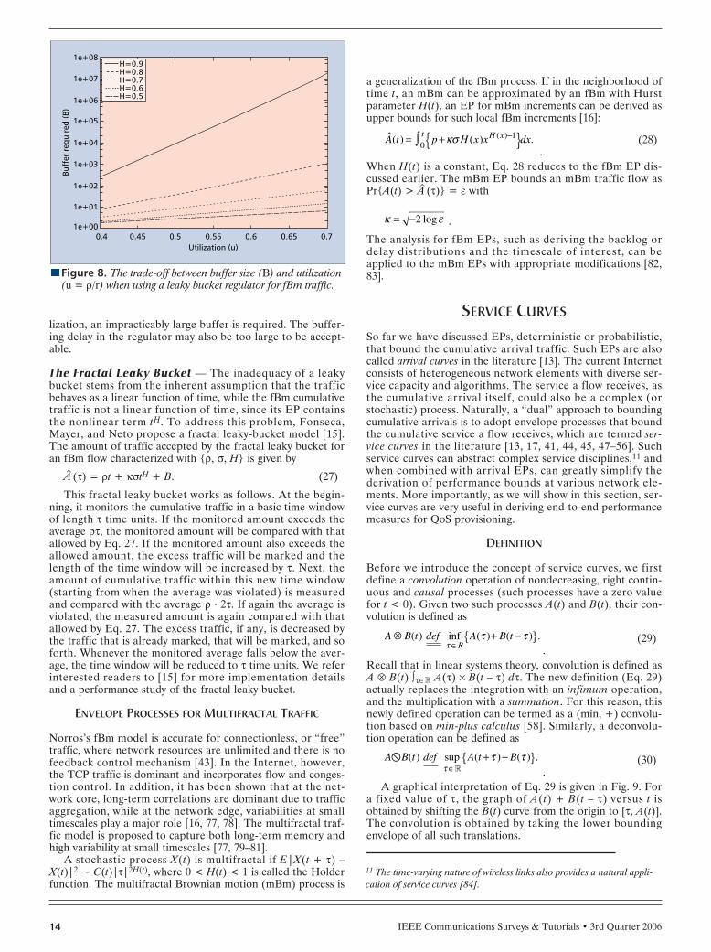
We conclude this article with a summary and qualitativecomparison of the EPs surveyed in this article, and a discus-sion on future research directions.


DETERMINISTIC ENVELOPE PROCESSES

In this section we review the class of deterministic EPs. Wefirst present the definition and properties of such EPs, andthen examine two representative deterministic EPs. Theirapplications in QoS provisioning is discussed and a perfor-mance study of such EPs is reviewed. Finally, we review theclass of work on the statistical multiplexing of deterministical-ly regulated flows.

DEFINITION

As discussed, envelope processses (EPs) are popular trafficmodels used to bound the traffic generated by user sessions[18, 19]. Consider a source generating traffic at rate a(t). Theamount of traffic generated in the time interval [t1, t2) is A(t1,t2) = ∫t1

t2 a(t)dt. For discrete-time systems, a(t) is the amountof arrival traffic in the t-th time slot, and the cumulative traf-fic during [t1, t2) is A(t1, t2) = Σt1

t2–1 a(t). Throughout this arti-

cle we consider stationary sources, that is, the statisticalcharacteristics do not change over time.

For such traffic flows, Cruz’s {σ, ρ} EP is defined as:

A(t2–t1) ≤ ρ ⋅ (t2 – t1) + σ, ∀t1 ≤ t2, (1)

where σ is the burstiness allowed, and ρ is an upper bound onthe long term average rate of the traffic flow [18]. Althoughthe cumulative traffic A(t1, t2) could have various forms, it isupper bounded by the deterministic function A (t2 – t1) = ρ ⋅(t2 – t1) + s during [t1, t2) for any t1 ≤ t2. Figure 1 illustratessuch an EP and the corresponding traffic flow. The EP can beshifted along the time axis from t = 0 to t = τ1 (or to t = τ2),while the cumulative arrival should always be upper boundedby the shifted functions. That is, the EP is only a function ofthe time interval τ = t2 – t1, regardless where the intervalbegins (i.e., t1).

Cruz’s EP is a simple linear function defined by twoparameters σ and ρ.1 In fact, a deterministic EP does not haveto follow such a specific form, and could be any nondecreas-ing, nonnegative function of time A (τ), as long as the cumula-tive traffic is bounded as follows [21]:

A(t1, t2) ≤ A (t2 – t1), ∀t1 ≤ t2. (2)

The choice for a specific A (τ) depends on how easy it is toenforc and analyze, and how tight it is in bounding the trafficflow (and thus how efficient it is in resource utilization). Wewill discuss examples of generalized deterministic EPs in the

following sections.

It is worth noting that for a given traffic flow, its EP is notunique. For example, if we have A(t) ≤ A (τ), then we haveA(t) ≤ k ⋅ A (τ) for any k > 1. For QoS provisioning, it istherefore important to examine the tightest one among all thebounding functions. It is shown in [21] that if A (τ) is increas-ing and subadditive,2 its long-term average rate ρ exists:

(3)

The limit ρ is referred to as the envelope rate of A (τ). Theminimum EP (i.e., the tightest bounding function) is called theminimum envelope process (MEP) of A(t) and is found to be

(4)

That is, A*(t) is the maximum amount of traffic that couldpossibly be generated by the given source in a time interval oflength t. It is shown in [21] that A*(t) is increasing and subad-ditive. The tightest bound on the average rate, ρ*, called theminimum envelope rate (MER), is the envelope rate of A*(t)[see Eq. 3].

THE {σ→, ρ→} ENVELOPE PROCESS

The {σ, ρ} EP has the advantages of being simple and easy toenforce with a token bucket. However, it is relatively loosebecause it enforces a burstiness constraint σ over all thetimescales, while typically a source tends to exhibits smallerburstiness over larger time-scales. For example, consider avariable bit rate (VBR) video source. The burstiness is largestat the timescale of a frame time. Its average bit rate over aninterval gradually decreases as the interval gets larger, and isequal to the long-term average rate at the timescale of theentire video trace length. For a given traffic process, a tighterEP indicates a more accurate estimate of the actual trafficload and implies that less network resources are required toaccommodate it. To achieve a high utilization, it is thus desir-able to use an EP that bounds the traffic over differenttimescales using different burstiness factors.

The discussion above suggests that a tighter traffic boundcan be obtained by deploying a concave, piecewise-linearenvelope. In [22, 31], the {σ, ρ} EP was extended to the {σ→,ρ→} EP, which maintains n {σ, ρ} pairs. The amount of trafficin a time interval t is restricted by A (t) = min1≤i≤n{σi + ρit}.Since each term σi + ρit is an affine function and the mini-mum of n affine functions is concave, A (τ) is concave andsubadditive.

Figure 2 illustrates such a {σ→, ρ→} EP, which consists offour linear segments and tightly bounds the arrival processA(t). The {σ→, ρ→} EPs can be enforced using a number of cas-caded leaky buckets, while a conforming flow keeps all theleaky buckets from overflowing. The T-SPEC in Intserv [5]adopts a dual leaky bucket model for traffic specification. Thecorresponding EP is A (τ) = min{M + Pt, B + rt}, where M,P, B, and r are parameters with constant values. This is a spe-cial case of the {σ→, ρ→} EP with n = 2.

D-BIND

Another piece-wise linear EP, D-BIND was introduced byKnightly et al. to address this multiple time-scale burstinessproblem in traffic flows [20]. To further illustrate this prob-

A t A s s ts

*( ) sup ( , ).= +≥0

ˆ limˆ( )

infˆ( )

.ρ defA t

t

A t

tt t→∞ ≥=

1

nFigure 1. Cruz’s {σ, ρ} Envelope Process A(t) = σ + ρ ⋅ t.

Envelopeprocess

A(t)

σ

ρ

A conformingtraffic flow

0 tτ1 τ2

1 An arbitrary traffic flow can be policed to be conforming to the {σ, ρ}EP by using a leaky bucket with a token rate ρ and a token bucket size σ. 2 A process A(t) is subadditive if A(t1 + t2) ≤ A(t1) + A(t2).


lem, consider the example in Fig. 3, which plots the arrivingprocess of an MPEG video trace with frame patternIBBPBBPBB. Usually, I frames have the highest rates and Bframes the lowest rates. It can be seen from this figure thatusing different bounds on the rate for different time intervalscan provide a tighter approximation for the traffic flow thanusing a single worst case bound for all the intervals.

Let Rk denote a data rate and Ik denote the correspondingtime interval. D-BIND was defined using multiple rate-inter-val pairs, {(Rk, Ik), k = 1, 2, …, K}, as the following piecewiselinear function:

(5)

where A (0) = 0 [20]. With Eq. 5, the rate Rk can be viewed asan upper bound on the session’s rate over any time interval oflength Ik, that is, A(t, t + Ik)/Ik ≤ Rk, ∀t > 0, k = 1, 2, …, K.

It is worth noting that the (σ, ρ) model may be viewed as aspecial case of the D-BIND model, since both are piecewiselinear functions. For both EPs, an important design parameteris K, the number of rate-interval (or {σ→, ρ→}) pairs to use.There is a trade-off between the tightness of the EP (whichdetermines the bandwidth utilization at network nodes) and K(which determines the complexity in shaping and policing).

Generally, the more rate-interval pairs used, the tighter thebound and therefore the higher the utilization (see the analy-sis in the next section). However, considering a typical corerouter where tens of thousands sessions are multiplexed, it isimpractical to use a large number of rate-interval pairs foreach session. Knightly et al. suggest that a source specify asmall number of rate-interval pairs (e.g., four or eight) forconnection admission control and policing [20]. We examinethis issue subsequently.

APPLICATIONS OF DETERMINISTIC EPS

Generally, the use of EPs is two-fold:• To simplify the enforcement of user traffic flows (e.g., by

adopting one or more leaky buckets) at the networkboundary

• To simplify the QoS provisioning in networksIn this section we discuss how to derive performance boundsand how to perform admission control using deterministicEPs. Their performance is discussed in the next section.

Performance Bounds — Consider a network element withservice rate c, modeled as a slotted-time single server G/G/1queue. At time slot t, the amount of arrival traffic is a(t).Under a work conserving policy,3 the backlog process q(t) ofthe queue is governed by the Lindley’s equation [59]:

q(t + 1) = max{0, q(t) + a(t) – c}. (6)

That is, the queue length in the next time slot is the currentqueue length increased by the traffic input a(t) and decreasedby the traffic being served during this slot. The maximumoperation is used, since the queue length should always benonnegative. It has been shown in [59] that the distribution ofq(t) determined by Eq. 6 converges to a unique limit distribu-tion as t → ∞, under some mild conditions [e.g., a(t) is station-ary and ergodic, and the average of a(t) should be less thanthe service capacity c].

Assuming the queue is empty at time 0, expanding Eq. 6recursively yields

q(t) = max{0, max{0, q(t – 2) + a(t – 2) – c} + a(t – 1) – c}= max {0, a(t – 1) – c, q(t – 2) + a(t – 1) + a(t – 2) – 2c}= …= max {0, a(t – 1) – c, …, a(t – 1) + a(t – 2) + … + a(0) – tc},

that is,

(7)

(8)

Eq. 7 conveniently relates the cumulative traffic A(t) to thequeue backlog.4 An upper bound on the backlog can bederived by substituting A(t) with its upper bounding approxi-mation A (τ) as in Eq. 8. Note that in Eq. 7, the right-hand-

q t a l t k ck t l k

t( ) max , ( ) ( )= − −

≤ < =

−∑

0

10

= − − −{ }≤ <

max , ( ) ( )0

0k t

A t k t k c

≤ − − −{ }≤ <

max , ˆ( ) ( ) .0

0k t

A t k t k c

ˆ( ) ( ) ,A tR I R I

I It I R I Ik k k k

k kk k k k= −

−− + ≤− −

−−

1 1

11 tt Ik≤ ,

nFigure 2. A piece-wise linear {σ→, ρ→} envelope process withthree {σ, ρ} pairs.

σ1

σ2

σ3

ρ1 ρ2 ρ3

0

A(t)

A(t)

t

nFigure 3. Burstiness of an MPEG video trace with a frame pat-tern of IBBPBBPBB.

I frames

B frames

P frames

A(t)

0 t

3 That is, the server will not be idle whenever traffic is backlogged.

4 For continuous time systems, we have q(t) = maxτ≤t{∫τta(t)dt – (t – τ)c}and q(t) = maxτ≤t{A(t – τ) – (t – τ)c} = maxs≤t{A(s) – sc}. This deriva-tion is similar to the discrete time system (where summation is replacedwith integration for continuous-time systems). In addition, this powerfulequation has been used to derive probabilistic bounds on QoS metrics.


side (RHS) consists of the random arrival process A(t), whilein Eq. 8, the RHS consists of a deterministic function A (τ).The analysis is greatly simplified by this substitution.

Based on Eq. 8, we can derive performance bounds onbacklog and delay for the network element as follows. Substi-tuting s = t – k into Eq. 8, we have [13]:

(9)

This is intuitive, since backlog is actually the amount of cumu-lative arrival decreased by the amount that has been served.

The delay bound depends on the specific service discipline.For a work conserving queue with any service discipline (e.g.,LCFS or FCFS), the delay of a traffic unit is upper boundedby the system busy period d. That is, since any backlog will beserved within d time units, the delay experienced by any trafficunit will be no larger than d. Clearly, d is the time intervalwhen the cumulative traffic arrival is equal to the cumulativeservice. An upper bound on d can be easily computed as [18,19, 35]:

d ≤ min {t : t ≥ 1 and A (t) – ct ≤ 0}. (10)

If the service discipline is FCFS, then a traffic unit will beserved after all the traffic arriving earlier than itself is cleared.This fact can be exploited to tighten the delay bound. Consid-er a traffic unit arriving at time t. Since it sees a backlog ofq(t), the delay it experiences will be the time it takes to servethe backlog q(t), that is, s such that q(t) – cs ≤ 0. We thenhave

d(t) ≤ min {s : s ≥ 1 and A (t) – c(t + s) ≤ 0}. (11)

These results can be further explained via an intuitivegraphical interpretation. In Fig. 4a, the queue becomes busyafter time 0. At time t1, the difference between the cumulativearrival and cumulative service is the amount of backlog in thequeue (i.e., q1). Since we use the deterministic EP to approxi-mate the traffic flow, an upper bound on the backlog is foundto be the difference between the EP and the cumulative ser-vice, (i.e., q2). By examining the graph, we can see that abound for the maximum backlog qmax occurs at time t2.

In Fig. 4b, when the real traffic-flow curve intersects withthe cumulative service curve at time d1, the queue becomesempty again. However, since we are using the deterministicEP to approximate the traffic flow, an upper bound on thebusy period is found to be the time instance when the EPintersects with the service curve (i.e., at d). In an FCFS queue,for a traffic unit arrives at time t3, the backlog it sees will becleared at time t4 (i.e., when the cumulative service is equal to

the cumulative arrivals at time t3). Therefore, its actual delayis d2, as shown in the figure. Since EP is used as an upperbound for the traffic flow, the upper bound on delay for thistraffic unit is d3.

According to the definition given by Eq. 2, there could bean arbitrary number of EPs for a given traffic flow. From theexamples in Fig. 4, it is easy to see that different EPs will givedifferent backlog and delay bounds for the same traffic flowand service capacity. As a result, tighter bounds on A(t) willalways be desirable for achieving more accurate performancebounds. In addition, the delay and backlog bounds are tight inthe sense that these bounds are realizable, since in the worstcase the cumulative arrival A(t) could be identical to A (τ),that is, the equality holds in Eq. 2. On the other hand, thesebounds are loose in the sense that they are the worst-case sce-narios that only occur rarely in most applications.

Admission Control Tests — The delay bound discussed inthe previous section can be used in admission control tests fordeterministic service. Admission control is used in networknodes to keep them from being overloaded. Usually an admis-sion control test is invoked when a new flow request arrives inorder to verify that, if the new flow is admitted, the QoSrequirements (e.g., a maximum acceptable delay) of existingflows and the new flow will all be satisfied. Otherwise, thenew flow request will be rejected.

The deterministic admission control test conditions for var-ious schedulers, that is, FCFS, static priority (SP), and earliestdeadline first (EDF), are presented in [18, 22, 60] and aresummarized in Table 1. These tests are used to verify if thedelay requirements of all the sessions (existing ones and thenew one) can be satisfied, and can be used to derive the maxi-mum number of user sessions with various deterministic delayrequirements that can be accepted at a network element(called the admissible region).

Consider an FCFS queue fed by N source flows, each con-forming to a deterministic EP A i(t), i = 1, …, N, and requir-ing a delay no larger than d. Let si be the maximum packetsize of the i-th flow. Since the scheduler does not distinguishbetween packets, the delay-bound test simply verifies that themaximum delay will not be larger than the delay requirementd. Suppose the queue is idle at time 0 and is busy thereafter.Since a traffic unit arriving at time t sees a backlog of ΣN

i=1A(t), its delay is the time it takes to clear the backlog and thelargest remaining service time of the packet that is beingserved at time t, max1≤i≤N si/c (since the service is not preemp-tive). Replacing the backlog with the sum of EPs will give theadmissible condition for the FCFS service discipline (see Eq.

q t A s scs t

( ) max { , ˆ( ) }.+ ≤ −< ≤

1 00

nFigure 4. A graphical interpretation of the backlog and delay bounds.

cEP

The realtraffic flow

EP

The realtraffic flow

c

A(t)

t1

q1

0 t

(a) Backlog bound (b) Delay bound

A(t)

t30 t

qmax

q2

t2 t5 d1

d2

d3

dt4


11).In SP systems, each traffic flow is assigned a priority level

p, 1 ≤ p ≤ P, according to their delay requirements dp. Usuallya higher-priority flow has a tighter delay requirement, that is,dp < dq, if p < q. The system maintains P FCFS queues, andtraffic belonging to the same priority level is put into the sameFCFS queue. When the server is available, it always serves thefirst packet in the nonempty FCFS queue with the highest pri-ority.

Let the set of flows with priority p be Cp, and the maxi-mum packet size for priority-p flows be sp

max. Consider a prior-ity-p packet arriving at time t. The packet will be served onlyafter the following two types of traffic are served:• The priority-p backlog at t (the first term on the RHS of

the test condition in Table 1) and• The higher-priority backlog and the higher-priority traffic

that arrived after t but before the tagged packet’s servicetime (the second term on the RHS of the test condition)

This is because such a packet arriving later than the priority-ppacket can still be served earlier due to its higher priority.Similarly, the last term on the RHS of the test condition is thelargest remaining service time of a lower priority packet thatis being served at time t.

In EDF, each packet is assigned a deadline (e.g., its arrivaltime plus its delay requirement). Packets in the queue aresorted according to their deadlines and the scheduler alwaysserves the packet with the smallest deadline [61]. EDF hasbeen shown to be optimal with respect to schedulability, in thesense that it can provide the highest level of deterministicdelay assurance among all scheduling disciplines [60, 62]. TheEDF schedulability condition in Table 1 can be interpreted asfollows. Consider a packet with delay requirement dj arrivingat time t – dj. The packet should be served before its deadlinet, which is possible if the maximum amount of traffic arrives

with a tighter deadline smaller than or equal to t, that is, ΣNi=1

A i (t – di) has been cleared before time t. The second term onthe RHS of the schedulability condition is again due to thefact that the packet currently in service cannot be preempted.

PERFORMANCE OF DETERMINISTIC ENVELOPE PROCESSES

For the class of deterministic EPs, there are two interestingquestions to be answered:• What is the best performance in utilizing network

resources that can be achieved using these EPs?• For the class of piecewise linear EPs, how many {σ, ρ}

pairs (or rate-interval pairs) are needed to achieve a uti-lization close to the best performance?These questions have been addressed in [22], via experi-

ments with VBR video traces. To answer the first question,the MEP (see Eq. 4) of MPEG video traces, termed empiricalenvelope in [22], is used in admission control tests. Since theempirical envelope is computed from a given video trace(Jurassic Park, MPEG encoded), it requires the entire trace apriori, and is hard to specify or police in practice. Neverthe-less, it is the tightest envelope for the specific video trace.Using empirical envelopes in admission control tests will yieldthe maximum number of acceptable sessions. This can serveas a benchmark for evaluating the performance of otherdeterministic EPs that are more practical.

The maximum number of admissible sessions using theoptimal EDF scheduler is given in Fig. 5a, as compared topeak rate allocation and average rate allocation [22]. It can beseen that the best utilization the deterministic EP can achieve(using the empirical envelope) lies between the peak rate allo-cation and the average rate allocation. Furthermore, the uti-lization increases when the delay constraint is relaxed.Although the utilization is low, compared to the average rate

nFigure 5. Performance of deterministic envelope processes [22]. 1996 IEEE.

Delay bound (milliseconds)

Average rate

Envelope

(a) Bandwidth utilization vs. delay tolerance

Peak rate

5000

20

Num

ber

of c

onne

ctio

ns

Ave

rage

uti

lizat

ion

40

60

80

100

120

1140

0.75

0.5

0.25

100 150 200 250 300 350 400 450 500

Delay bound (milliseconds)

(b) Bandwidth utilization vs. complexity of the EPs

1 (σ,ρ) pair

6 (σ,ρ) pairs

2 (σ,ρ) pairs

7 (σ,ρ) pairs Envelope/ 8 (σ,ρ) pairs

3/4/5 (σ,ρ) pairs

5000

10

Num

ber

of c

onne

ctio

ns

Ave

rage

uti

lizat

ion

20

30

40

50

60

0.1

0.2

0.3

0.4

100 150 200 250 300 350 400 450 500

nTable 1. Delay bound tests for FCFS, EDF, and SP packet scheduler [22].

Scheduler Condition

FCFS d ≥ Σi=1N A i (t)/c – t + max1≤ i≤N si /c, for all t ≥ 0.

Static Priority ∃τ ≤ dp : t + τ ≥ Σi∈Cp A i(t)/c + Σq=1p–1 Σi∈Cq A i(t + τ)/c – t + maxr>psr

max/c, for all p, t ≥ 0.

EDF t ≥ Σi=1N A i(t – di)/c + maxdi>t si /c, for all t ≥ d1.


allocation, there is still significant improvement of peak rateallocation, especially when the delay constraint is relaxed. Forexample, utilizations ranging from 15 to 30 percent areachievable for a delay bound of 30 ms. This is because in theworst case that all the sessions are transmitting at their peakrates, the excess traffic can be buffered briefly, as long as theirdelay constraints are met. The more relaxed the delay con-straints are, the longer they can be buffered; hence, the small-er service capacity required.

To answer the second question, Fig. 5b in [22] presents theutilization achieved by several {σ→, ρ→} EPs having differentnumbers of {σ, ρ} pairs, where the maximum utilizationachieved by the empirical envelope serves as a benchmark.The general trend in Fig. 5b is that the greater the number of{σ, ρ} pairs, the higher the utilization, since a session requiresless capacity when a more accurate approximation (i.e., atighter upper bound) is used in admission control. Anotherinteresting observation is that the additional improvement inutilization decays quickly when more {σ, ρ} pairs are used.This implies that reasonably high utilization, as compared tothe benchmark, can be achieved by using a relatively smallnumber of {σ, ρ} pairs.

STATISTICAL MULTIPLEXING OF REGULATED SOURCES

Statistical Multiplexing — The experimental studies in [22](see the previous section) provide an idea about the bestdeterministic performance guarantees that can be achieved byusing deterministic EPs (i.e., using the tightest envelope —MEP, and the optimal scheduling discipline — EDF). Inorder to achieve higher utilization, statistical multiplexingmust be explored. On the other hand, deterministic EPs arestill highly attractive due to the fact that they are amenable toenforcement. Therefore, a natural solution is statistical multi-plexing of deterministically regulated flows. A statistical servicecan improve upon a deterministic service by taking advantageof the statistics of individual source, and the statistical inde-pendence of the source traffic flows. Note that independenceof the source flows is the most fundamental assumption forthe following results.

A simple example is given in Fig. 6. Figure 6a plots a dis-crete-time, periodic on–off source: it generates one unit oftraffic in time slot 1, and then can be silent for the remainingnine time slots, and so forth. Multiplexing N such sources(with identical phases), we get an aggregate traffic flow whichis on in time slot 1 and off in the remaining nine time slots,and the aggregate peak rate is N, as shown in Fig. 6b. Howev-er, if the sources have independent, random phases (e.g.,source 1 is on in time slot 1, while source 2 is on in time slot5, and so forth), the aggregate traffic is actually smoothed out,as shown in Fig. 6c. The aggregate rate a(t) fluctuates slightly

around the average rate N × 1/10. A direct result of thisobservation is that the amount of resources required to sup-port QoS for N traffic flows will be much smaller than Ntimes the resource required to support QoS for a single trafficflow.

It is worth noting that even with random phases, it is stillpossible that the worst-case scenario in Fig. 6b will occur, butsuch events only occur rarely. If we perform admission controlaccording to the “average” or more likely case (i.e., Fig. 6c), asignificant improvement in resource utilization can beachieved. When the worse-case scenario happens, there willbe a violation of the QoS requirements. Through rigorousmodeling and analysis, however, we can guarantee that such aviolation occurs with low probability (e.g., 10–6).

Related Work — The analysis work along this line generallytakes two steps. First, find the worst-case traffic flow, generat-ed by the so-called adversarial sources, that maximizes theresources required (in the hard QoS guarantee case) or theQoS violation probability (in the soft QoS guarantee case),which, however, still conforms to the deterministic EP. Suchadversarial sources are extremal, periodic on-off processeswith a random phase for bufferless multiplexers [26, 63]. Forbuffered multiplexers, the adversarial traffic pattern is foundto be periodic, with multiple “on” phases and a different ratein each “on” phase [63–65]. Second, take advantage of therandom phases of the adversarial sources and multiplex themstatistically.

In [23], admission control for a network node with finitebuffer B and capacity C is studied. The joint allocation ofbuffer and capacity is first reduced to a single resource alloca-tion problem by the notion of a virtual buffer/trunk system.Then the derived single resource allocation problem is solvedby applying the known results on bufferless multiplexing,where the Chernoff Bound [66] is used to estimate the lossprobability.

In [28], it was found that there is no benefit in resourcesharing for lossless multiplexing. Furthermore, for determinis-tic QoS guarantees, there is a unique timescale determined bythe system parameters and the input flows, which determinesthe optimal buffer/bandwidth trade-off. For statistical multi-plexing, [28] transforms the two-resource allocation probleminto two independent single-resource allocation problems,which is shown to achieve higher multiplexing gain than [26].

In [29], the multiplexer was examined under the more gen-eral {σ→, ρ→} EP. An interesting result in [29] is that althoughthe extremal, periodic on-off source is adversarial for a buffer-less multiplexer, it is not adversarial for the transformed two-resource allocation problem. In [31], a bufferless multiplexingsystem is studied, in which each regulated flow is firstsmoothed by a smoother with a capacity that is determined by

nFigure 6. An illustration of statistical multiplexing gain.

Time slot (t)1000

01000

a(t)

20003000400050006000700080009000

1000011000

200 300 400 500 600Time slot (t)

10000

500

a(t)

1000

1500

200 300 400 500 600

(a) A discrete-time, periodic on-off source (b) The rate a(t) of aggregating 10000 such sources with identical phase

(c) The rate a(t) of aggregating 10000 such sources with random phases

a(t)

1

1

2 11 t10


the delay requirement of that source. This novel structureenables end-to-end statistical guarantees [30], since thebufferless multiplexer ensures that a flow still keeps the samedescription after leaving the system. There is no need toimplement per-node traffic shaping [27] with this framework.

In [23], local and global effective envelopes for the aggre-gate regulated flows are constructed using the ChernoffBound and the Central Limit Theorem (CLT) [67]. Applyingthe effective envelopes in admission control tests furtherimproves the admissible region [23, 68]. More details on effec-tive envelopes are provided below.

Finally, a multiplexer with general flows is studied in [24]using a CLT approach and in [25] using large deviation theo-ry, respectively. Although these papers do not assume regulat-ed flows, their results can be applied to the multiplexing ofregulated flows. The maximum variance bounds in [24] isfound to achieve the highest utilization, as compared to sever-al other approaches in a comparison study of admission con-trol schemes [12].

PROBABILISTIC ENVELOPE PROCESSES

PROBABILISTIC ENVELOPE PROCESSES ANDSOFT QOS GUARANTEES

In the previous section we discussed deterministic EPs whichcan be used for provisioning of deterministic or “hard” perfor-mance guarantees, such as worst-case delay bounds and nopacket dropped in the network. Generally, such deterministicservices are quite conservative since they are based on worst-case analysis [22]. In addition, hard performance guaranteesmight be an overkill for many applications, say, multimediacommunications, where a certain amount of loss or delay vio-lation is tolerable.

As opposed to the deterministic service approach, a statis-tical service provides probabilistic service assurances. Forexample, such “soft” QoS guarantees can be in the followingforms:

Pr {delay ≥ d} ≤ ε or Pr {loss ≥ l} ≤ ε, (12)

where ε is the probability that the delay or loss bound d or l isviolated and is generally dependent on the specific applica-tion.

By allowing a fraction of traffic to violate its QoS require-ment, a user can trade-off the QoS he receives with the net-work resources required. More importantly, such aprobabilistic approach can significantly increase networkresource utilization. In the previous section, we have seen sig-nificant improvements when statistical multiplexing isexplored, even though each source is deterministically regulat-ed. An alternative approach in soft QoS provisioning is to usethe class of probabilistic EPs that bound traffic flows in aprobabilistic manner. In the following, we will survey repre-sentative probabilistic EPs and the probabilistic QoS guaran-tees they provide.

BOUNDED BURSTINESS PROCESSES

Definition — The piecewise linear EPs discussed in the previ-ous section extend the {σ, ρ} EP by using multiple {σ, ρ}pairs. Both classes of EPs bound the flows deterministically,(i.e., Eq. 2 always holds true). Another dimension of extend-ing Cruz’s work is to allow the EPs to be violated (i.e., lettingEq. 2 hold true in a probabilistic sense). The cumulative traf-fic A(t) is allowed to exceed its EP A (τ), but with a probabili-ty decaying with the degree that the EP is exceeded. This class

of EPs are known as the Bounded Burstiness Processes [32].Let F be the set of functions f(σ) such that for any order n,

the n-fold integral

is bounded for any σ > 0. An arrival process A(t) has astochastically bounded burstiness (SBB) with upper rate ρ andbounding function f(σ) if• f(σ) ∈ F; and• Pr{A(s, t) ≥ ρ (t – s) + σ} ≤ f(σ), for all σ ≥ 0 and all t ≥ 0.

As will become clear shortly, the first condition in the SBBdefinition is required for the closure property: a traffic flow(or its description) will not explode as it travels through onenetwork node after another. Also note that the finiteness ofthe n-fold integral implies that f(σ) is a decaying function(otherwise the integral from σ to ∞ will not exist). The secondcondition specifies that the probability that A(t) exceeds the{σ, ρ} EP decays with f(σ): the larger the σ, the smaller theviolation probability.

Furthermore, a stochastic process q(t), that is, the backlogprocess, is stochastically bounded (SB) with bounding functionf(σ) if• f(σ) ∈ F; and• Pr{q(t) ≥ σ} ≤ f(σ), for all σ ≥ 0 and all t ≥ 0.

As in the SBB definition, the first condition above is alsorequired for the closure property. The second condition in theabove definition specifies that the probability that q(t) exceedsσ (i.e., the probability that the backlog is larger than σ)decays with f(σ): the larger the σ, the smaller the violationprobability.

Since f(σ) is general in both definitions, one can choosedifferent forms of f(σ) for traffic flows with different charac-teristics. For example, an exponential bounding function canserve a good model for short range dependent (SRD) trafficflows,5 while the sum of exponentials or a Weibullian bound-ing function can be used to characterize LRD traffic thatexhibits burstiness over multiple timescales.

The SBB Calculus — Based on the above definitions,Starobinski and Sidi present a network calculus for SBB pro-cesses [32], which is very useful in analyzing a feedforwardnetwork6 with SBB arrivals, such as proving the stability ofsuch networks and deriving QoS performance measures.7 TheSBB calculus is summarized in the following.

Summation — Let Ai(t) be SBB with {ρi, fi(σ)}, i = 1, 2.Then the sum of these two SBB processes A1(t) + A2(t) is alsoSBB with {ρ1 + ρ2, g(σ)}, where g(σ) = f1(pσ) + f2((1 – p)σ)and p is any real number in (0, 1).

This result is derived via some basic properties of randomvariables. Consider two random variables X1 and X2. For aconstant x, the set of events that {X1 + X2 ≥ x} is a subset of{X1 ≥ px} ∪ {X2 ≥ (1 – p)x}, for all 0 < p < 1. Therefore, the

… ∞∞ ∫∫ σσn times

nf u du

1 24 34

( )( )

5 An SRD process has an autocorrelation function that decays exponen-tially.

6 A feedforward network is a network in which there are no cycles in thegraph generated by the routes of various sessions. This concept depends onboth the topology of the network and the routing scheme applied.

7 A queueing network is stable if the queues do not increase withoutbound, that is, limσ→∞Pr{qi ≥ σ} = 0, where qi corresponds to the steady-state workload in the i-th network element.


probability of the former event should be no larger than thatof the latter, that is, Pr{X1 + X2 ≥ x} ≤ Pr{[X1 ≥ px] ∪ [X2 ≥(1 – p)x]}. Since the probability of the union of two events isupper bounded by the sum of the probabilities of the twoevents, we have Pr{(X1 + X2) ≥ x} ≤ Pr{X1 ≥ px} + Pr{X2 ≥(1 – p)x}. Now if both X1 and X2 are SBB, substituting thedefinition in the previous section, we get the summationresult. Note that the derivation does not require the twosources be independent.

Characterization — For a work-conserving system with ser-vice rate ρ, if the backlog q(t) is SB with bounding functionf(σ), that is, Pr{q(t) ≥ σ} ≤ f(σ), then the input process of thesystem is SBB with upper rate ρ and the same bounding func-tion f(σ), that is, Pr{A(t – s) ≥ ρ(t – s) + σ} ≤ f(σ).

This result shows the relation between the input processand the backlog process. It is derived from the Lindley’s equa-tion. From Eq. 7, we have q(t) ≥ A(t – s) – (t – s)c. From theSB definition, we have Pr{A(t – s) – (t – s)c ≥ σ} ≤ f(σ), whichgives the characterization result.

Calculus for an Isolated Network Element — For a workconserving queueing network element with service rate c, ifthe input process A(t) is SBB with {ρ, f(σ)}, then the outputprocess B(t) is SBB with {ρ, g(σ)}, where g(σ) = f(σ) +{1/c–ρ} ∫σ∞ f(µ)dµ, and the backlog process q(t) is SB with thesame bounding function g(σ).

The proof of these results is more mathematically involved.We omit the proof here and refer interested readers to [42] formore details. There are several interesting implications fromthese results. First, if exogenous inputs to a network with work-conserving elements are SBB, then all the traffic flows withinthe network are SBB and all the backlogs in the network ele-ments are SB (i.e., the closure property is conserved). Second,the SBB calculus is quite general, since there is no assumptionmade on flow independence and scheduling disciplines (exceptthat the servers are work-conserving). On the other hand, if fur-ther information on scheduling and independence is available, afiner analysis may result in better performance bounds [32, 42].

Third, the last result gives the backlog distribution, that is,SB with g(σ) if the arrival process is SBB with {ρ, f(σ)}. Thiscan serve as a good approximation of loss probability for finitebuffer systems [69]. Other performance measures such as delaydistribution can also be derived from this result. Finally, theSBB calculus greatly simplifies the analysis of any feedforwardnetwork fed by external SBB processes, since the end-to-endanalysis can be reduced to the analysis of each isolated nodealong the route inductively. Also note that every time when aflow traverses a network element, there will be an additionalintegration over [σ, ∞) on the bounding function. For the traf-fic flow to remain bounded after traversing n network ele-ments, the n-fold integral of f(σ) should be bounded (see thedefinition of SBB and SB earlier in this section). More discus-sion on end-to-end analysis will be presented later.

Exponential Bounded Burstiness — Exponential BoundedBurstiness (EBB) processes are SBBs with a bounding func-tion f(σ) = φe–ασ, where φ and α are source-specific constants[33]. With this definition, the probability that the input pro-cess exceeds the linear EP A (τ) = ρt + σ decays exponential-ly or faster than exponentially. Obviously, this is true for allSRD traffic.

Interesting results on EBB calculus have been establishedin [33]. In addition, since no independence assumption isrequired when applying the analysis in [33], both feedforwardnetworks and general cyclic networks can be analyzed. Perfor-mance of a GPS server (and a GPS network) with EBB ses-

sions can be found in [70].

Sum of Exponentials — This is a more general class ofbounded burstiness processes than EBB. A Sum of Exponen-tials Bounded Burstiness process has a bounding function inthe form of the summation of a number of exponentials, thatis, f(σ) = ΣK

k=1 φk e–αkσ, where φk and αk are constants, for k= 1, …, K [32]. The motivation behind this model is the exis-tence of multiple timescales in network traffic and the obser-vation that, on logarithmic scale, the delay distribution in amultiplexer can be roughly broken into two linear regions,called the cell region and the burst region [71]. Using multipleexponential bounds on the tail distribution of a queue cancapture this multiple timescale phenomenon and provide atighter bound than EBB.

One problem with the calculus of sums of exponentials is thatthe number of exponentials required to bound the burstiness of aprocess within the network grows each time the process mergeswith another process (i.e., summation). As a result, this trafficmodel does not have the closure property. In [32], Starobinskiand Sidi present an ad hoc procedure, which provides a simpleway to derive bounding functions using the sum of two exponen-tials, but at the cost of lower accuracy.

Another interesting example of SBB is the Weibull BoundedBurstiness Processes (WBB), which has a Weibullian boundingfunction [34, 42]. Since WBB also belongs to the the class ofEPs for self-similar traffic, we present its discussion later in thisarticle.

CHANG’S LOG-MOMENT GENERATING FUNCTION BOUNDS

In addition to bounding the burstiness of a traffic flow, proba-bilistic QoS guarantees can also be achieved by deterministi-cally bounding the moment generating function of A(t) [21].8Consider a random variable X. If its moment-generating func-tion is bounded by a finite constant ψ as E(eθX) ≤ ψθ, thenfrom the Chernoff bound [66], its distribution is boundedexponentially with respect to θ as:

Pr{X ≥ x} ≤ ψθ e–θx, for all x > 0. (13)

Since the cumulative arrival A(t) is a random variable, itsmoment generating function can thus be bounded by a deter-ministic function A (θ, t) as follows:

(14)

where A (θ, t) is called an EP of A(t) with respect to θ [21]. Asin the deterministic case, the MEP of A(t) is A*(θ, t) =sups≥0{(1/θ)log E exp [θA (s, s + t)]}, and the MER of A(t) isa*(θ) = lim supt→∞A*(θ, t)/t. It is shown in [21] that the MERof A(t) is an increasing function of θ: from the mean rate tothe peak rate, as θ increases from 0 to ∞.

Applying the Chernoff bound Eq. 13 and the Lindley’sequation (Eq. 6), the log-moment generating function EP canbe used to derive QoS performance measures at a networkelement. Consider a queue fed by a flow with a linear EP,A (τ) = ρ(θ)t + σ(θ). Assume ρ(θ)< c to make a stable sys-tem. We have the following interesting results from [21]:

Backlog Distribution — The total backlog q(t) is boundedexponentially with respect to θ, that is, Pr{q(t) ≥ x} ≤ β(θ)e–θx,where β(θ) is a constant.

11 2

2 1 1 2θθθlog ˆ( , ), ,( , ) Ee A t t t tA t t ≤ − ∀ ≤

8 The moment-generating function of a random variable X is defined to bethe expectation of eθX, that is, E{eθX}.


Delay Distribution — If the FCFS scheduling policy is used,the delay distribution is also bounded exponentially as Pr{d(t)≥ d} ≤ eθρ(θ) β(θ)e–θc(d–1).

Input–Output Relationship — The departure process b(t)has an MEP B^(θ, t) ≤ ρ(θ)t + 1/θ logβ(θ). The departure pro-cess still has the same long-term average rate as the input pro-cess, but with a possibly different burst factor.

Again, there is the closure property: if the input processesto such a network have their log-moment generating functionsbounded, then every process in the network (e.g., delay, back-log) and the arrival processes at internal nodes has an expo-nentially bounded distribution. These are useful results forsoft QoS guarantees, from which one can estimate how muchnetwork resources (e.g., buffer or bandwidth) are required toachieve a desired buffer overflow probability (or a delay dis-tribution), and conveniently trade-off the QoS violation prob-ability and the network resource required.

KUROSE’S BOUNDS

In [35], Kurose presented a framework for soft QoS provision-ing, which is based on EPs with a family of bounding randomvariables. With this framework, a traffic flow is characterizedby a family of random variables {B(t1), B(t2), …} that stochas-tically bounds the source over the respective interval lengthstk, k = 1, 2, ….

Such a bounding approach is somewhat similar to D-BIND, where multiple rate-interval pairs are used to boundthe cumulative arrival A(t). The important difference here isthat the D-BIND EP will not be violated, while Kurose’s EPbounds the traffic flow in a probabilistic manner. More specif-ically, a random variable X is said to be stochastically largerthan a random variable Y (denoted as X fst Y) if and only ifPr{X > x} ≥ Pr{Y > x} for all x [72]. Therefore, in the defini-tion of Kurose’s bounds, the cumulative traffic in any timeinterval tk is stochastically bounded by the corresponding ran-dom variable B(tk), that is, Pr{B(tk) > x} ≥ Pr{A(τ, τ + tk} >x), or B(tk) fst A(τ, τ + tk), ∀τ.

Consider an FCFS multiplexer with a link speed of c andserving N flows. Each flow is characterized by its respectivefamily of bounding random variables. A stochastic bound onthe delay in this system is shown to be

(15)

where β is an upper bound on the busy period and is the small-est nonnegative value such that Σi=1

N |Bi(β)| ≤ cβ [35]. An intu-itive explanation of Eq. 15 is that if the backlog seen by a taggedpacket [see Lindley’s equation (Eq. 8)] is larger than cd, then itwill take the FCFS server more than d time units to clear thebacklog before serving the tagged packet, and the delay boundof the tagged packet will be thus violated in this case.

When the input is bounded by a set of random variable-time interval pairs, the output traffic of a work-conservingnetwork element is also bounded by the same set of randomvariables, but over a different (smaller) interval of time. Withthis result, we can derive a flow’s characterizations along thehops from its ingress point to the network node being studied.Heuristic algorithms are presented in [35] to compute end-to-end delay guarantees on a per-session basis, which, however,usually give loose results as compared with simulation. Fur-thermore, to use Eq. 15, we need to compute the convolutionof N random variables for each time interval tk, which resultsin a high computation complexity [36].

H-BINDThe Hybrid Bounding Interval Dependent (H-BIND)approach provides statistical QoS guarantees by exploiting therandom phases of deterministically constrained flows [20, 36].In H-BIND, each session is regulated by a D-BIND EP and alarge number of flows are multiplexed at a network element.When computing the delay distribution using Eq. 15, thebounding random variables, Bi(tk), are assumed to be Gaus-sian (reasonable when the number of flows is large), which isfully determined by its mean and variance [67]. For Bi(tk), themean is calculated from the source’s D-BIND EP. Since thereare many arrival processes that conform to a D-BIND EP, thevariance σ2(tk) is computed using the arriving process thatmaximizes it (i.e., an adversarial source).

In [20], Knightly also extended the FCFS stochastic boundin Eq. 15 to the static priority case. Let there be P priorities,Cp be the set of flows with priority level p, and the delayrequirement for priority p connections be dp. Then the delayviolation probability for a priority-p packet is bounded by [20]:

(16)

where βp is a bound on the priority-p busy period. This is sim-ilar to the deterministic admission control test for static prior-ity systems discussed earlier. However, the RHS of Eq. 16now provides a bound on the delay distribution of priority-ptraffic.

For H-BIND, the Gaussian assumption eliminates the con-volution computation required when Kurose’s bound is used.Such an approximation can be quite accurate, considering thelarge number of flows multiplexed at a core router. Moreover,when used for admission control, H-BIND achieves band-width utilization of up to 86 percent in a realistic scenario[36], which is much higher than the 15 to 30 percent band-width utilization achievable with deterministic EPs [22]. Suchsigificant gain is due to the fact that statistical multiplexing isexplored in H-BIND. In addition, the D-BIND/H-BINDframework allows for the simultaneous support of hard andsoft QoS guarantees. With this framework, all the sources areconstrained by D-BIND EPs. Sources demanding determinis-tic service are served with higher priority than sources choos-ing statistical service.

It is also worth noting that H-BIND is essentially a single-multiplexer analysis. In [20], Knightly discusses how to extendthis analysis to derive end-to-end performance bounds. SinceH-BIND explores statistical multiplexing gain, flow indepen-dence is an important assumption, which may not hold truewhen flows share a common buffer.9 Knightly suggests adopt-ing delay-jitter control (or the simpler rate-jitter control) atevery network node, which decouples the network nodesalong an end-to-end path by reconstructing the sources’ origi-nal traffic pattern at each hop [73, 74]. With this technique, ifa delay bound dh is provided at hop h with violation probabili-ty εh, the end-to-end delay violation probability is found to bePr{De2e > Σdh} ≤ Πεh [20].

RATE VARIANCE ENVELOPE PROCESSES

Pr{ } max Pr ( ),D d B tp pt

p i kik

p

> ≤ +

≤ ≤ ∈∑

0 β C

B t d ct cdq i k p k piq

p

p

, ( )+ − ≥

∈=

−∑∑

C1

1

,

Pr{ } max Pr ( )D d B t ct cdt

i ki

N

kk

> ≤ − ≥

≤ ≤ =∑

0 1β

,

9 This problem is solved in [31] by adopting bufferless multiplexing sys-tems.


Rather than bounding the cumulative traffic A(t) itself, theRate Variance EPs are used to bound the statistical proper-ties of A(s, s + t) as a function of the interval length t [36, 37].The rate-variance of a flow,

(17)

describes the variance of a stream’s arrival rate over intervalsof length tk. This characterization captures the second momentcorrelation structure of an arrival process. Note that it makesno assumption on A(t) and allows for an arbitrary autocorrela-tion structure of individual sessions. Using video traces asexamples, Knightly [36] shows that the RV(tk) curves of thevideo traces can be bound or approximated using two or threepiecewise linear segments on the log-log scale.

For admission control tests, the Rate Variance EP of theaggregate traffic Σi Ai(s, s + tk) can be approximated using aGaussian Envelope with variance Σi tk2RVi(tk) over intervals oflength tk. That is, the summations in the RHS of Eqs. 15 and16 can be approximated with Gaussian random variables andthe probabilities computed using a Gaussian distribution withthe corresponding mean and variance.

The Rate Variance EPs have been shown to achieve veryhigh utilization in [12] as compared to other methods. Howev-er, it is more difficult to enforce a flow to follow such EPs.Reference [75] presents a measurement-based admission con-trol scheme based on Rate Variance EPs, where the maximalrate envelope of the aggregate flow is adaptively measuredover the currently admitted flows.

EFFECTIVE ENVELOPES

The class of effective envelopes are functions which upperbound multiplexed traffic with high certainty [23]. As in H-BIND, the traffic flows are assumed to be deterministicallyregulated, e.g., by piecewise linear deterministic EPs, and pos-sess several general properties, such as stationarity, indepen-dence, additivity and subadditivity.

Two types of effective envelopes are defined in [23], name-ly, a local effective envelope and a global effective envelope.Consider a set of flows C with arrival functions Ai(t). Theaggregate traffic is AC(t, t + τ) = ΣC Ai(t, t + τ). The localeffective envelope that upper bounds AC(t, t + τ) is a functionGC(.;ε) that satisfies

Pr{AC(t, t + τ) ≤ GC(τ; ε)} ≥ 1 – ε, ∀τ ≥ 0 and ∀t. (18)

That is, a local effective envelope upper bounds the aggregatetraffic for any specific (“local”) time interval of length τ [23].Furthermore, it is a probabilistic bound: the aggregate trafficis allowed to exceed the local effective envelope, but with asmall probability (at most, ε).

Global effective envelopes are defined for the same aggre-gate traffic AC(t, t + τ), but are bounds for the arrival in allsubintervals [t, t + τ) of a larger interval. More precisely, aglobal effective envelope for an interval of length β is a subad-ditive function HC(.; β; ε) such that

Pr{EC(τ;β) ≤ HC(τ;β;ε), ∀0 ≤ τ ≤ β} ≥ 1 – ε, (19)

where EC(τ;β) is the empirical envelope of AC(t, t + τ), and βcould be an upper bound on the largest system busy period.HC(τ; β; ε) is a bound for traffic for all subintervals of length τ≤ β in the interval β, which is more stringent than local effec-tive envelopes and leads to more conservative admission con-trol [23].

For a given set of flows Ai(t) and their correspondingdeterministic EPs A i(t), the effective envelopes can be com-

puted as follows [23]. First, the bound on the moment gener-ating function of an individual flow is computed, which isfound to be a function of the corresponding deterministic EPA i(t). Due to the independence assumption, the bound on themoment generating function of the aggregate traffic flow,MC(s, τ), can be easily derived, as the product of those of theindividual flows. Second, applying Chernoff bound [see Eq.13], we have

Pr{AC(0, τ) ≥ Nx} ≤ e–NxsMC(s, τ). (20)

Substituting the moment generating bound derived in the firststep, the local effective envelope can be obtained by solvingfor Nx from Eq. 20.

Once the local effective envelope is derived, Boorstyn et al.use a geometric argument to construct the global effectiveenvelope HC from the local effective envelope GC. Specifically,they show that HC can be bounded by GC from both sides as

GC(τ;ε) ≤ HC(τ;β;ε) ≤ GC(τ′; ε′), (21)

where τ′/τ > 1 and ε′/ε < 1 depend on the interval β. It hasbeen shown that for ε sufficiently small and β not too large,τ′/τ ≈ 1, and the resulting global effective envelope is reason-ably close to the local effective envelope.

Effective envelopes thus derived can be applied to providestatistical service assurances for various traffic schedulingalgorithms. In the following we use FCFS as an example;other scheduling disciplines such as static priority or EDF canbe derived similarly and we refer interested readers to [23] forthese results. The schedulability condition for FCFS with astatistical delay service Pr{D ≥ d} ≤ ε is

(22)

where t – τ is the last time before t that the queue is empty.That is, when a tagged traffic unit arrives at time t, it sees abacklog of sup τ {AC(t – τ , t) – cτ } [see the Lindley’s equation(Eq. 8)]. To provide the required statistical service, the proba-bility that the server can clear this backlog in d time unitsshould be no smaller than 1 – ε. Furthermore, this schedula-bility condition can be approximated by10

(23)

From the definition Eq. 18, GC(τ;ε) < x implies that Pr{AC(t, t+ τ) > x} < ε. Consequently, the schedulability condition canbe rewritten as

(24)

When the global effective envelope is used in admission con-trol test, the schedulability condition is found to be

(25)

which has a similar structure to Eq. 24.Finally, we use Fig. 7 from [23] to illustrate the perfor-

mance of several EPs discussed thus far in admission control.In this example two classes of flows are multiplexed at a net-work element with a service rate of 45 Mb/s. The delaybounds are 100 and 10 ms for Class 1 and 2 flows, respective-ly, and the delay violation tolerance is chosen to be ε = 10–6.

sup ( ˆ; ; ) ˆ ,τ

τ β ε τHC −{ } ≤c cd

sup ( ˆ; ) ˆ .τ

τ ε τGC −{ } ≤c cd

supPr ( ˆ, ) ˆ ,τ

τ τ εA t t c cdC − − ≤{ } ≥ −1

Pr sup{ ( , ) ˆ} ,τ

τ τ εA t t c cdC − − ≤

≥ −1

RV t def VarA s s t

tk Kk

k

k( )

( , ), , , , ,

+

= …1 2

10 This approximation is accurate if the arrivals follow a Gaussian process[12, 23]. For general cases, the left-hand side (LHS) of Eq. 23 is an upperbound for the LHS of Eq. 22.


The admissible regions obtained with various EPs and thestatic priority and EDF scheduling algorithms are plotted inFig. 7.

In Fig. 7, the admissible regions of peak rate allocationand average rate allocation serve as benchmarks. The admissi-ble region of any feasible algorithm should fall in betweenthese two regions. We can see the admissible region of deter-ministic service is much larger than that of peak rate alloca-tion. This is because with deterministic service, when theinstantaneous aggregate rate is large than c, the extra trafficcan be temporarily buffered, as long as they are served beforetheir delay deadlines. It can also be observed that the schemesthat explore statistical multiplexing gain, that is, EB-EMW[26], EB-RRR [29], Bufferless MUX [31], and local and glob-al effective envelopes [23], achieve much larger admissibleregions (indicating high bandwidth utilizations). The admissi-ble regions for other probabilistic EPs that do not exploit sta-tistical multiplexing gains, such as SBB, EBB, and Chang’slog-moment generation bounds (although not shown in thefigure), are expected to lie between the deterministic servicecurve and the EB-EMW curve in Fig. 7.

ENVELOPES FOR SELF-SIMILAR TRAFFIC

Since the seminal work [40], many empirical studies haveshown that network data and video traffic are LRD or self-similar in that they exhibit high burstiness over multipletimescales [38, 39, 41]. In [43], Norros introduces a frameworkto model the connectionless data traffic using fractal Browni-an motion (fBm) models. This framework inspire the WeibullBounded Burstiness EPs [34, 42] and is the basis for the fBmEP [15].

WEIBULL BOUNDED BURSTINESS PROCESSES

In the past decade, tremendous effort has been made to buildtraffic models that not only model the statistical aspect of self-similar traffic, but also are manageable for traffic engineering.The sum of exponentials model tries to model the LRD char-acteristics within the traditional Markovian analysis paradigm,while some other traffic models have been proposed to modelLRD and self-similarity in a more direct manner.

Previous work, such as [43, 76], shows that a single serverFCFS queue fed by self-similar traffic, such as fBm traffic, hasa Weibullian asymptotic tail. Motivated by this finding, and ina way analogous to the EBB model, the Weibull Bounded

Burstiness (WBB) traffic model is proposed for fBm trafficflows [34, 42].

Weibull Bounded (WB) and WBB processes with Hurstparameter H are defined as a special type of SBB, with aWeibullian bounding function f(σ) = φe–ασ2(1–H), where φ iscalled the asymptotic constant and α the decay rate. This isconsistent with [76] that showed that the buffer overflowprobability of an FCFS queue fed with fBm traffic has thesame form as f(σ). Since WBB processes belong to the classof SBB processes, the SBB calculus can also be applied toWBB processes. Analytical results for GPS systems with WBBtraffic flows can be found in [34].

THE FBM EP

Consider a Brownian motion (BM) process A(t) with mean ρand variance σ2, an EP A (t) that tightly bounds this process isfound to be A (τ) = ρt + κσt{1/2}, where κ determines theprobability that A(t) exceeds A (τ) at time t, that is, if Pr{A(t)> A (t)} = ε, then [67]:

.This approach can be extended to deal with fBm traffic.

Consider an fBm traffic flow AH(t) with mean ρ, variance σ2,and Hurst parameter H. Fonseca, Mayor, and Neto [15] pre-sent an fBm EP that bounds this fBm process:

A H(t) = ρt + κσtH, for 1/2 ≤ H ≤ 1. (26)

Similarly, here κ also determines the probability that AH(t)exceeds A H(t) at time t, that is, if Pr{AH(t) > A H(t)} = ε,then

.

Equation 26 has a similar format as Cruz’s EP A (τ) = ρt + σ:a constant rate process increased by a burst factor. But theburst factor is a constant in Cruz’s EP, while an increasingfunction of t in Eq. 26. Such a burst factor captures the burstynature of fBm arrival processes.

As in the effective envelope case, given a small ε, we cancompute an EP which is exceeded by the traffic flow withprobability ε. The computation is however much simpler, sincewe only need to set

in Eq. 26. It is also worth noting the similarity between thedefinition of fBm EPs and that of local effective envelopes(Eq. 18). As a result, the schedulability conditions developedfor local effective envelopes (e.g., Eq. 24) can also be used forfBm EPs for statistical service assurances. Furthermore, thiscondition is exact (rather than an approximation), since thetraffic flow is Gaussian [12, 23].

THE FRACTAL LEAKY BUCKET

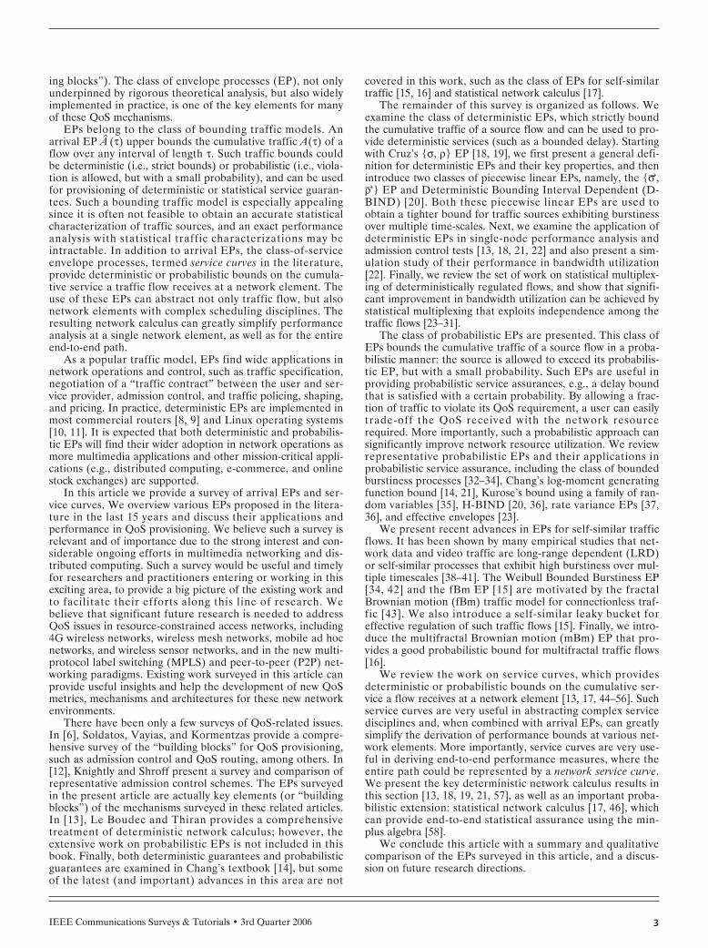
The Inadequacy of the Leaky-Bucket Regulator — Anideal leaky-bucket regulator should accept all conformingpackets, but drop or mark nonconforming packets. It is shownin [15] that it is very hard to choose the leaky-bucket parame-ters regulating an fBm traffic flow. A set of chosen parame-ters either gives low utilization, or results in extremely largebuffer and delay.

As an example, Fig. 8 plots the buffer size required, B,under various utilizations, defined as the ratio of the meanrate of the fBm traffic ρ to the long-term rate of the leaky-bucket regulator r, that is, u = ρ/r. It can be seen that Bincreases exponentially with u. To achieve an acceptable uti-

κ ε= −2 log

κ ε= −2 log

κ ε= −2 log

nFigure 7. Admissible region of multiplexing Class 1 and Class2 flows with ε = 10–6, delay deadlines d1 = 100 ms, and d2 =10 ms [23]. 2000 IEEE.

Number of class-2 connections500

0

50Num

ber

of c

lass

-1 c

onne

ctio

ns

100

150

200

250

300

100

BufferlessMUX

EB-RRREB-EMW

150

Peakrate

Deterministic

Average rate

Global eff. env. (LW)

Local eff. env. (CLT)

Local eff. env. (CB)

Global eff. env.

200

For local and global eff. env.: Thick lines = EDF scheduling

Thin lines = SP scheduling

250 300


lization, an impracticably large buffer is required. The buffer-ing delay in the regulator may also be too large to be accept-able.

The Fractal Leaky Bucket — The inadequacy of a leakybucket stems from the inherent assumption that the trafficbehaves as a linear function of time, while the fBm cumulativetraffic is not a linear function of time, since its EP containsthe nonlinear term tH. To address this problem, Fonseca,Mayer, and Neto propose a fractal leaky-bucket model [15].The amount of traffic accepted by the fractal leaky bucket foran fBm flow characterized with {ρ, σ, H} is given by

A (τ) = ρt + κσtH + B. (27)

This fractal leaky bucket works as follows. At the begin-ning, it monitors the cumulative traffic in a basic time windowof length τ time units. If the monitored amount exceeds theaverage ρτ, the monitored amount will be compared with thatallowed by Eq. 27. If the monitored amount also exceeds theallowed amount, the excess traffic will be marked and thelength of the time window will be increased by τ. Next, theamount of cumulative traffic within this new time window(starting from when the average was violated) is measuredand compared with the average ρ ⋅ 2τ. If again the average isviolated, the measured amount is again compared with thatallowed by Eq. 27. The excess traffic, if any, is decreased bythe traffic that is already marked, that will be marked, and soforth. Whenever the monitored average falls below the aver-age, the time window will be reduced to τ time units. We referinterested readers to [15] for more implementation detailsand a performance study of the fractal leaky bucket.

ENVELOPE PROCESSES FOR MULTIFRACTAL TRAFFIC

Norros’s fBm model is accurate for connectionless, or “free”traffic, where network resources are unlimited and there is nofeedback control mechanism [43]. In the Internet, however,the TCP traffic is dominant and incorporates flow and conges-tion control. In addition, it has been shown that at the net-work core, long-term correlations are dominant due to trafficaggregation, while at the network edge, variabilities at smalltimescales play a major role [16, 77, 78]. The multifractal traf-fic model is proposed to capture both long-term memory andhigh variability at small timescales [77, 79–81].

A stochastic process X(t) is multifractal if E|X(t + τ) –X(t)|2 ~ C(t)|τ|2H(t), where 0 < H(t) < 1 is called the Holderfunction. The multifractal Brownian motion (mBm) process is

a generalization of the fBm process. If in the neighborhood oftime t, an mBm can be approximated by an fBm with Hurstparameter H(t), an EP for mBm increments can be derived asupper bounds for such local fBm increments [16]:

.(28)

When H(t) is a constant, Eq. 28 reduces to the fBm EP dis-cussed earlier. The mBm EP bounds an mBm traffic flow asPr{A(t) > A (τ)} = ε with

.

The analysis for fBm EPs, such as deriving the backlog ordelay distributions and the timescale of interest, can beapplied to the mBm EPs with appropriate modifications [82,83].

SERVICE CURVES

So far we have discussed EPs, deterministic or probabilistic,that bound the cumulative arrival traffic. Such EPs are alsocalled arrival curves in the literature [13]. The current Internetconsists of heterogeneous network elements with diverse ser-vice capacity and algorithms. The service a flow receives, asthe cumulative arrival itself, could also be a complex (orstochastic) process. Naturally, a “dual” approach to boundingcumulative arrivals is to adopt envelope processes that boundthe cumulative service a flow receives, which are termed ser-vice curves in the literature [13, 17, 41, 44, 45, 47–56]. Suchservice curves can abstract complex service disciplines,11 andwhen combined with arrival EPs, can greatly simplify thederivation of performance bounds at various network ele-ments. More importantly, as we will show in this section, ser-vice curves are very useful in deriving end-to-end performancemeasures for QoS provisioning.

DEFINITION

Before we introduce the concept of service curves, we firstdefine a convolution operation of nondecreasing, right contin-uous and causal processes (such processes have a zero valuefor t < 0). Given two such processes A(t) and B(t), their con-volution is defined as

.(29)

Recall that in linear systems theory, convolution is defined asA ⊗ B(t) ∫τ∈¡ A(τ) × B(t – τ) dτ. The new definition (Eq. 29)actually replaces the integration with an infimum operation,and the multiplication with a summation. For this reason, thisnewly defined operation can be termed as a (min, +) convolu-tion based on min-plus calculus [58]. Similarly, a deconvolu-tion operation can be defined as

.(30)

A graphical interpretation of Eq. 29 is given in Fig. 9. Fora fixed value of τ, the graph of A(t) + B(t – τ) versus t isobtained by shifting the B(t) curve from the origin to [τ, A(t)].The convolution is obtained by taking the lower boundingenvelope of all such translations.

A B t def A t Bx ( ) ( ) ( ) . supτ

τ τ∈

+ −{ }¡

A B t def A B tR

⊗ + −{ }∈

( ) ( ) ( ) . infτ

τ τ

κ ε= −2 log

ˆ( ) ( ) .( )A t p H x x dxH xt= +{ }−∫ κσ 10

11 The time-varying nature of wireless links also provides a natural appli-cation of service curves [84].

nFigure 8. The trade-off between buffer size (B) and utilization(u = ρ/r) when using a leaky bucket regulator for fBm traffic.

Utilization (u)0.450.4

1e+00

1e+01

Buff

er r

equi

red

(B)

1e+02

1e+03

1e+04

1e+05

1e+06

1e+07

1e+08

0.5 0.55 0.6 0.65 0.7

H=0.9H=0.8H=0.7H=0.6H=0.5


Now we are ready to define the service curve for a networkelement [45]. Consider a network element serving a cumula-tive traffic flow of A(t) and generate an output process ofB(t). A causal process S is a minimum service curve if thedeparture process satisfies B(t) ≥ A ⊗ S(t), and a causal pro-cess S

–is a maximum service curve if B(t) ≤ A ⊗ S–(t). Thus S(t)

provides a lower bound on the cumulative service the trafficflow receives, while S

–(t) provides an upper bound on the

cumulative service the traffic flow receives. This is analogousto linear systems such as a low-pass filter, where the responseis the convolution of the input signal and the impulse responseh(t) of the system.

APPLICATION OF SERVICE ENVELOPES FORDETERMINISTIC SERVICE GUARANTEES

Among the two types of service curves, minimum servicecurves play a larger role in service assurance since, combinedwith arrival EPs, they can provide upper bounds on the QoSperformance measures. Consider a network element withcumulative arrival EP A (d) and a minimum service curve S(t).As illustrated in Fig. 10, the maximum delay dmax is equal tothe maximum horizontal distance between the two curves, themaximum backlog qmax is equal to the maximum vertical dis-tance between the two curves, and the time instance when thetwo curves intersect d provides an upper bound on the systembusy period.

This collection of results, including the input/output char-acterization, is termed deterministic network calculus [13, 18,19, 21, 50, 57]. We use the notation in [17] and summarize thekey results in the following. Consider a network element witha minimum service curve S(t). The cumulative arrival A(t) isbounded by its deterministic EP A (t), and the cumulativedeparture process is B(t). The following hold:• Output Envelope: The function B(t) = AxS(t) is an enve-

lope for the departure process, in the sense that, for all t,τ ≥ 0,

B(t + τ) – B(τ) ≤ B(t). (31)

• Backlog Bound: An upper bound for the backlog, denotedby qmax, is given by

qmax = AxS(0). (32)

• Delay Bound: An upper bound for the delay, denoted bydmax, is given by

dmax = inf{d ≥ 0 | ∀t ≥ 0 : A (t – d) ≤ S(t)}. (33)

Given the notion of service curve, these results can be easi-ly extended to end-to-end performance bounds. For example,consider the guaranteed service adopted by the IETF Intservworking group [5]. The source describes the offered traffic interms of an arrival EP and requests a lossless service with afixed upper bound on end-to-end delay. Each of the routersalong the path allocates network resources (bandwidth andbuffers) to serve this session. Such a service can be modeledas a flow traversing a sequence of service curve elements [45].

Let there be n network elements. Each element i has aminimum service curve Si(t), a maximum service curve S

–i(t), is

fed by the departure process Bi–1(t) from the upstream ele-ment, and generates a departure flow of Bi(t). Consider theoutput of the last network element Bn(t). From the definitionof minimum service curves, we have

Bn(t) ≥ Bn–1 ⊗ Sn(t)≥ (Bn–2 ⊗ Sn–1) ⊗ Sn(t)≥ …≥ A ⊗ (S1 ⊗ S2 ⊗ … ⊗ Sn)(t).

Similarly, for the maximum service curves, we can obtain Bn(t)≤ A ⊗ (S

–1 ⊗ S

–2 ⊗ … ⊗ S

–n)(t).

Let Snet(t) =def S1 ⊗ S2 ⊗ … ⊗ Sn(t) and S–net =def S

–1 ⊗ S

–2 ⊗ …

⊗ S–

n(t). With the use of service curves, not only the serviceprocess at a network element can be abstracted, but also thethe entire path (or the network cloud) can be modeled with aminimum network service curve Snet(t) and a maximum net-work service curve S

–net(t). End-to-end performance boundscan be easily computed by plugging in the network servicecurves into Eqs. 31, 32, and 33, as in the single-network-ele-ment analysis.

STATISTICAL NETWORK CALCULUS

As in the arrival EP case, service curves can also be used tobound the service a flow receives in the probabilistic sense.This approach has been explored by several researchers. In[85], Cruz introduces a probabilistic service curve which allowsviolations according to a certain distribution. A statistical net-work calculus for the class of “dynamic F-servers” was hintedat in [14], and a family of “statistical service envelopes” isdefined in [53] to lower bound the service received by anaggregated flow.

In [17], Burchard, Liebeherr, and Patek define a (mini-mum) effective service curve, given by

Pr{B(t) ≥ A ⊗ Sε(t)} ≥ 1 – ε. (34)

nFigure 9. A graphical interpretation of the convolution opera-tion A ⊗ B(t).

A(t)

A B(t)

0

A(τ1)

A(τ2)+B(t-τ2)

A(τ1)+B(t-τ1)A(τ2)

tτ1 τ2

nFigure 10. A graphical interpretation of maximum delay andbacklog using the arrival EP and minimum service curve.

A(t)/S(t)

Arrival EP

0

Maxbacklog

Maxdelay

Minimumservice curve

tt1 dt2


The effective service curve Sε(t) bounds the service a singleflow receives with high certainty. Using effective servicecurves, a set of statistical network calculus results are devel-oped in [17]. We use the notation in [17] and summarize themain results in the following. Given an arrival process A(t)conforming to a deterministic EP A (t), and given an effectiveservice curve Sε(t), the following hold:

• Output Envelope: The function AxSε(t) is a probabilisticbound for the departures on [0, t], in the sense that, forall t, τ > 0,

Pr{B(t, t + τ) ≤ AxSε(τ)} ≥ 1 – ε. (35)

• Backlog Bound: A probabilistic bound for the backlog isgiven by qmax = AxSε(0), in the sense that, for all t > 0,

Pr{q(t) ≤ qmax} ≥ 1 – ε. (36)

• Delay Bound: A probabilistic bound for the delay is givenby dmax = inf{d ≥ 0 | ∀t ≥ 0: A (t – d) ≤ Sε(t)}, in thesense that, for all t > 0,

Pr{d(t) ≤ dmax} ≥ 1 – ε. (37)

Furthermore, consider a flow A(t) that traverses K networkelements in series, each having an effective service curveSk,ε(t). Then, for any t ≥ 0,

(38)

where a > 0 is an arbitrary parameter, and δτ(t) is an impulsefunction which is ∞ for t > τ and 0 for t ≤ τ.

It is worth noting that when ε = 0 (and by letting a → 0 inEq. 38), these results reduce to the deterministic network cal-culus discussed in the previous section. These are elegant andimportant results for end-to-end statistical QoS provision. Werefer interested readers to [17] for proofs and other details,and to [46, 51] for the latest advances along this line of work.

CONCLUDING REMARKS

In this article we have surveyed various EPs proposed in theliterature over the past 15 years, as well as their applicationsin QoS provisioning. The EPs we have discussed include theclass of deterministic EPs for deterministic service assurance,the class of probabilistic EPs for statistical service assurance,the class of EPs for self-similar traffic flows, the class of ser-vice curves. We also reviewed the results from deterministicnetwork calculus and statistical network calculus.

A summary and qualitative comparison of the EPs exam-ined in this article are provided in Table 2. These EPs differin many aspects and their efficiency and accuracy heavilydepend on the traffic assumptions. Generally, deterministicEPs are appealing because they are simple in implementation,while probabilistic EPs are more efficient in utilizing networkresources. Furthermore, statistical multiplexing can achievesignificant improvement in resource utilization, especiallywhen the number of flows is large. Indeed, statistical multi-plexing is very useful in a number of contexts, including bothwired and wireless networks. Therefore, a promising directionis to use deterministic EPs to regulate flows at the networkedge, and statistically multiplex regulated flows within the net-work for statistical service assurance. Although it is also possi-ble to statistically multiplex flows regulated by probabilisticEPs, the margin for further improvement may be small. As

can be seen from Fig. 7, statistical multiplexing of determinis-tically regulated flows has already achieved a utilization veryclose to that of average rate allocation.

Currently there is considerable ongoing research on QoSissues in several new networking environments, such as wire-less access networks (including 4G wireless networks, wirelessmesh networks, mobile ad hoc networks, and wireless sensornetworks), MPLS networks, and P2P networks. These net-works bring about some interesting problems and unique diffi-culties for QoS provisioning. For example, a wireless link hasa time-varying capacity subject to fading and interference,which is quite different from wired links with a fixed capacity.Wireless transmissions also suffer high loss rates due to trans-mission errors, which is also quite different from Internetlinks where buffer overflow is considered as the main cause ofloss. Furthermore, user mobility also introduces more fre-quent topology change in such networks. As another example,the logical topology in a P2P network is quite different fromthe traditional “edge-core” architecture under which mostQoS mechanisms/architectures are developed. How to adaptQoS mechanisms in such environments still remains open,since all these issues need to be addressed in the problem for-mulation.

Another promising direction for future research is cross-layer design and optimization. Most existing QoS mechanismsare developed under the layered protocol architecture.Although leading to simple independent implementations, this“layered” approach also results in suboptimal application per-formance. Breaking the barrier among the layers, combinedwith jointly optimizing the QoS mechanisms/operations acrossmultiple layers (e.g., directly optimizing multimedia replayquality via the resource management, adaptation, control, andprotection strategies available at the lower layers of the stack)has the potential of “squeezing the most” out of resource-con-strained wireless networks, which are much more unreliablethan their wired counterparts. We believe this survey can beuseful for research efforts along these directions.

ACKNOWLEDGMENTS

The authors are grateful to the editor, Dr. Martin Reisslein,and the seven anonymous reviewers whose commentsimproved the quality of this article. This work has been sup-ported in part by the National Science Foundation undergrants CNS-0520054, CNS-0435303, and CNS-0435228, and bythe New York State Office of Science, Technology and Aca-demic Research (NYSTAR) through the Center for AdvancedTechnology in Telecommunications (CATT) at PolytechnicUniversity.

REFERENCES[1] K. Asatani, H. Ueda, and C. M. Lockhart, “Voice over IP and

Quality of Service,” Guest Editorial, IEEE Commun. Mag., vol.42, no. 7, July 2004.

[2] R. Chandramouli et al., Guest Editorial, “Recent Advances inWireless Multimedia,” IEEE JSAC, vol. 21, no. 10, Dec. 2003.

[3] N. L. S. da Fonseca and P. Shenoy, Guest Editorial, “Proxy Sup-port for Streaming in the Internet,” IEEE Commun. Mag., vol.42, no. 8, Aug. 2004.

[4] S. Blake et al., “An Architecture for Differentiated Services,”IETF RFC2457, Dec. 1998.

[5] R. Braden, D. Clark, and S. Shenker, “Integrated Services in theInternet Architecture: An overview,” IETF RFC 1633, July 1994.

[6] J. Soldatos, E. Vayias, and G. Kormentzas, “On the BuildingBlocks of Quality of Service in Heterogeneous IP Networks,”IEEE Commun. Surveys and Tutorials, vol. 7, no. 1, 1st Quarter2005, pp. 70–89.

[7] J. Liebeherr, “Post-Internet QoS Research,” IWQoS 2004 Panel

Pr ( ) ( ), ,( )B t A S S tKK a≥ ⊗ ⊗ ⊗ ⊗( ){ }−

11

ε ε δL

≥ − + −

1 1 1ε ( )Kt

a

,


Speech, Montreal, Canada, June 2004.[8] Cisco IOS Documentation, “QC: Cisco IOS Release 12.0, Quality

of Service Solutions Configuration Guide,” http://www.cisco.com/

[9] Juniper Networks, Inc., http://www.juniper.net/[10] W. Almesberger, “Traffic Control–Next Generation: Reference

Manual,” http://linux-ip.net/ gl/tcng/[11] D. K. Y. Yau and X. Chen, “Resource Management in Soft-

ware Programmable Router Operating Systems,” IEEE JSAC,vol. 19, no. 3, Mar. 2001 pp. 488–500.

[12] E. Knightly and N. Shroff, “Admission Control for StatisticalQoS: Theory and practice,” IEEE Network, vol. 13, no. 2, Mar.1999, pp. 20–29.

[13] K. Kumaran et al., “Novel Techniques for the Design andControl of Generalized Processor Sharing Schedulers for Multi-ple QoS classes,” Proc. IEEE INFOCOM’00, Tel-Aviv, Israel, Mar.2000, pp. 932–41.

[14] C. S. Chang, Performance Guarantees in Communication Net-works, London: Springer Verlag, 2000.

[15] N. L. S. da Fonseca, G. S. Mayor, and C. A. V. Neto, “On theEquivalent Bandwidth of Self-Similar Sources,” ACM Trans.Modeling and Computer Simulation, vol. 10, no. 2, Apr. 2000,pp. 104–24.

[16] C. A. V. Melo and N.L.S. da Fonseca, “An Envelope Processfor Multifractal Traffic Modeling,” Tech. Rep. IC-03-21, Univer-sidade Estadual de Campinas, Nov. 2003.

[17] A. Burchard, J. Liebeherr, and S. D. Patek, “A Calculus for

End-to-End Statistical Service Guarantees (2nd revised ver-sion),” Tech. Rep. CS-2001-19, University of Virginia, May2002.

[18] R.L. Cruz, “A Calculus for Network Delay, Part I: Network Ele-ments in Isolation,” IEEE Trans. Info. Theory, vol. 37, no. 1,Jan. 1991, pp. 114–31.

[19] R. L. Cruz, “A Calculus for Network Delay, Part II: NetworkAnalysis,” IEEE Trans. Info. Theory, vol. 37, no. 1, Jan. 1991,pp. 132–41.

[20] E. W. Knightly, “H-BIND: A New Approach to Providing Statis-tical Performance Guarantees to VBR Traffic,” Proc. IEEE INFO-COM’96, San Francisco, CA, Mar. 1996, pp. 1091–99.

[21] C.-S. Chang, “Stability, Queue Length, and Delay of Deter-ministic and Stochastic Queueing Networks,” IEEE Trans. Auto-matic Control, vol. 39, no. 5, May 1994, pp. 913–31.

[22] D. E. Wrege et al., “Deterministic Delay Bounds for VBRVideo in Packet-Switching Networks: Fundamental Limits andpractical Trade-Offs,” IEEE/ACM Trans. Net., vol. 4, no. 3, June1996, pp. 352–62.

[23] R. R. Boorstyn et al., “Statistic Service Assurances for TrafficScheduling Algorithms,” IEEE JSAC, vol. 18, no. 12, Dec. 2000,pp. 2651–64.

[24] J. Choe and N. B. Shroff, “A Central Limit Theorem basedApproach to Analyze Queue Behavior in ATM Networks,”IEEE/ACM Trans. Net., vol. 6, no. 5, Oct. 1998, pp. 659–71.

[25] M. Montgomery and G. De Veciana, “On the Relevance ofTimescales in Performance Oriented Traffic Characterization,”

nTable 2. A summary of the EPs discussed in this article.

Whatis bounded

Stat.multiplexing

Det. or stat.service

Considersself-sim.?

Implementationcomplexity

Utilizationperformance

{σ, ρ} EP A(t) No Deterministic No Low Low

{σ→, ρ→} EPs A(t) No Deterministic No Low Low

D-BIND A(t) No Deterministic No Low Low

Stat. mux. of regulated flows Σ i Ai (t) Yes Statistical No High High

SBB A(t) No Statistical No Medium Medium

EBB A(t) No Statistical No Medium Medium

Sum of exponentials A(t) No Statistical Yes Medium Medium

Chang’s bounds 1/θlog EeθA(t1, t2) No Statistical No Medium Medium

Kurose’s bounds Σ i Ai (t) Yes Statistical No High Medium

H-BIND Σ i Ai (t) Yes Statistical No High High

Rate variance EPs Yes Statistical No High High

Effective envelopes Σ i Ai (t) Yes Statistical No High High

WBB A(t) No Statistical Yes Medium Medium

fBm EPs A(t) No Statistical Yes Medium High

mBm EPs A(t) No Statistical Yes Medium High

Det. service curves B(t) N/A Det./Stat. N/A Low Low

Prob. service curves B(t) N/A Statistical N/A High High

VarA s s t

ti k

k

( , )+


Proc. IEEE INFOCOM’96, San Francisco, CA, Apr. 1996, pp.513–20.

[26] A. Elwalid, D. Mitra, and R. H. Wentworth, “A New Approachfor Allocating Buffers and Bandwidth to Heterogeneous Regu-lated Traffic in an ATM Node,” IEEE JSAC, vol. 13, no. 6, Aug.1995, pp. 1115–27.

[27] L. Georgiadis et al., “Efficient Network QoS Provisioningbased on Per Node Traffic Shaping,” IEEE/ACM Trans. Net., vol.4, no. 4, Aug. 1996, pp. 482–501.

[28] F. Lo Presti et al., “Source Time Scale and OptimalBuffer/Bandwidth Trade-off for 39 Heterogeneous RegulatedTraffic in an Network Node,” IEEE/ACM Trans. Net., vol. 7, no.4, Aug. 1999, pp. 490–501.

[29] S. Rajagopal, M. Reisslein, and K.W. Ross, “Packet Multiplex-ers with Adversarial Regulated Traffic,” Proc. IEEE INFO-COM’98, San Francisco, CA, Mar./Apr. 1998, pp. 347–55.

[30] M. Reisslein, K. W. Ross, and S. Rajagopal, “GuaranteeingStatistical QoS to Regulated Traffic: The Multiple Node Case,”Proc. IEEE CDC’98, Tempa, FL, Dec. 1998, pp. 531–38.

[31] M. Reisslein, K. W. Ross, and S. Rajagopal, “A Framework forGuaranteeing statistical QoS,” IEEE/ACM Trans. Net., vol. 10,no. 1, Feb. 2002, pp. 27–42.

[32] D. Starobinski and M. Sidi, “Stochastically Bounded Bursti-ness for Communication Networks,” IEEE Trans. Info. Theory,vol. 46, no. 1, Jan. 2000, pp. 206–121.

[33] O. Yaron and M. Sidi, “Performance and Stability of Commu-nication Networks via Robust Exponential Bounds,” IEEE/ACMTrans. Net., vol. 1, no. 3, June 1993, pp. 372–85.

[34] X. Yu et al., “Queueing Processes in GPS and PGPS with LRDTraffic Inputs,” IEEE/ACM Trans. Net., vol. 13, no. 3, June2005, pp. 676–89.

[35] J. Kurose, “On Computing Per-Session Performance Bounds inHigh-Speed Multi-hop Computer Networks,” Proc. ACM SIG-METRICS’92, New Port, RI, June 1992, pp. 128–139.

[36] E. W. Knightly, “Enforceable Quality of Service Guarantees forBursty Traffic Streams,” Proc. IEEE INFOCOM’98, San Francisco,CA, Mar./Apr. 1998, pp. 635–42.

[37] E. W. Knightly, “Second Moment Resource Allocation inMulti-Service Networks,” Proc. ACM SIGMETRICS’97, Seattle,WA, June 1997, pp. 181–91.

[38] J. Beran et al., “Long-Range Dependence in Variable-Bit-Ratevideo traffic,” IEEE Trans. Commun., vol. 43, no. 2, Feb. 1995,pp. 1566–79.

[39] M. Garrett and W. Willinger, “Analysis, Modeling and Gener-ation of Self-Similar VBR Video Traffic,” Proc. ACM SIG-COMM’94, London, U.K., Aug. 1994, pp. 265–79.

[40] W. E. Leland et al., “On the Self-Similar Nature of EthernetTraffic,” IEEE/ACM Trans. Net., vol. 2, no. 1, Feb. 1994, pp.1–15.

[41] V. Paxson and S. Floyd, “Wide-Area Traffic: The Failure ofPoisson Modeling,” IEEE/ACM Trans. Net., vol. 3, no. 3, June1995, pp. 226–44.

[42] D. Starobinski, Quality of Service in High Speed Networkswith Multiple Time-Scale Traffic, Ph.D. dissertation,Technion–Israel Institute of Technology, May 1999.

[43] I. Norros, “On the Use of Fractional Brownian Motion in theTheory of Connectionless Networks,” IEEE JSAC, vol. 13, no. 6,Aug. 1995, pp. 953–62.

[44] R. Agrawal and R. Rajan, “Performance Bounds for Guaran-teed and Adaptive Services,” Tech. Rep. RC20649, IBMResearch Division, Yorktown Heights, NY, 1996.

[45] R. Agrawal et al., “Performance Bounds for Flow Control Pro-tocols,” IEEE/ACM Trans. Net., vol. 7, no. 3, June 1999, pp.310–23.

[46] F. Ciucu, A. Burchard, and J. Liebeherr, “A Network ServiceCurve Approach for the Stochastic Analysis of Networks,” Proc.ACM SIGMETRICS’05, Banff, Alberta, Canada, June 2005, pp.279–90.

[47] R. L. Cruz, “Quality of Service Guarantees in Virtual CircuitSwitched Networks,” IEEE JSAC, vol. 13, no. 6, Aug. 1995, pp.1048–56.

[48] P. Goyal, S. S. Lam, and H. M. Vin, “Determining End-to-EndDelay Bounds in Heterogeneous Networks,” Multimedia Sys-tems, vol. 5, no. 3, May 1997, pp. 157–163.

[49] A. Hung and G. Kesidis, “Bandwidth Scheduling for Wide-

Area ATM Networks using Virtual Finishing Times,” IEEE/ACMTrans. Net., vol. 4, no. 1, Feb. 1996, pp. 49–54.

[50] J.-Y Le Boudec, “Application of Network Calculus to Guaran-teed Service Networks,” IEEE Trans. Info. Theory, vol. 44, no.3, May 1998, pp. 1087–96.

[51] C. Li, A. Burchard, and J. Liebeher, “A Network Calculus withEffective Bandwidth,” Tech. Rep. CS-2003-20, University of Vir-ginia, Nov. 2003.

[52] A. K. Parekh and R. G. Gallager, “A Generalized ProcessorSharing Approach to Flow Control in Integrated Services Net-works: The Multiple Node Case,” IEEE/ACM Trans. Net., vol. 2,no. 2, Apr. 1994, pp. 137–50.

[53] J.-Y. Qiu and E. W. Knightly, “Inter-Class Resource Sharingusing Statistical Service Envelopes,” Proc. IEEE INFOCOM’99,New York, NY, Apr. 1999, pp. 1404–11.

[54] H. Sariowan, R. L. Cruz, and G. C. Polyzos, “Scheduling forQuality of Service Guarantees Via Service Curves,” Proc. IEEEICCCN’95, Las Vegas, NV, Sept. 1995, pp. 512–20.

[55] H. Sariowan, A Service-Curve Approach to Performance Guar-antee in Integrated-Service Networks, Ph.D. dissertation, Uni-versity of California at San Diego, June 1996.

[56] D. Stiliadis and A. Varma, “Latency-Rate Servers: A GeneralModel for Analysis of Traffic Scheduling Algorithms,” IEEE/ACMTrans. Net., vol. 6, no. 5, Oct. 1998, pp. 611–24.

[57] C. S. Chang, “On Deterministic Traffic Regulation and ServiceGuarantees: A Systematic Approach by Filtering,” IEEE Trans.Info. Theory, vol. 44, no. 3, May 1998, pp. 1097–110.

[58] F. Baccelli et al., Synchronization and Linearity: An Algebrafor Discrete Event Systems, New York: Wiley, 1992.

[59] R. M. Loynes, “The Stability of a Queue with Non-Indepen-dent Inter-Arrival and Service Times,” Proc. Cambridge Philos.Soc., vol. 58, no. 3, 1962, pp. 497–520.

[60] J. Liebeherr, D. Wrege, and D. Ferrari, “Exact Admission Con-trol for Networks with Bounded Delay Services,” IEEE/ACMTrans. Net., vol. 4, no. 6, Dec. 1996, pp. 885–901.

[61] D. Ferrari and D. C. Verma, “A Scheme for Real-Time ChannelEstablishment in Wide-Area Networks,” IEEE JSAC, vol. 8, no.3, Apr. 1990, pp. 368–79.

[62] L. Georgiadis, R. Guerin, and A. Parekh, “Optimal Multiplex-ing on a Single Link: Delay and Buffer Requirements,” IEEETrans. Info. Theory, vol. 43, no. 6, Sept. 1997, pp. 1518–35.

[63] B. T. Doshi, “Deterministic Rule based Traffic Descriptors forBroadband ISDN: Worst Case Behavior and Connection Accep-tance Control,” Proc. ITC’94, Antibes–Juan-les-Pins, France,June 1994, pp. 591–600.

[64] G. Kesidis and T. Konstantopoulos, “Extremal Traffic andWorst-Case Performance for Queues with Shaped Arrivals,”Proc. Wksp. Analysis Simulation Commun. Networks, Toronto,Canada, Nov. 1998.

[65] G. Kesidis and T. Konstantopoulos, “Extremal Shape-Con-trolled Traffic Patterns in High-Speed Networks,” IEEE Trans.Commun., vol. 48, no. 5, May 2000, pp. 813–19.

[66] H. Chernoff, “A Measure of Asymptotic Efficiency for Tests ofa Hypothesis based on the Sum of Observations,” AnnalsMath. Statist., vol. 23, 1952, pp. 493–507.

[67] A. Papoulis and S. U. Pillai, Probability, Random Variables,and Stochastic Processes, 4th ed., New York: McGraw-Hill,2002.

[68] C. Oottamakorn, S. Mao, and S. S. Panwar, “On GeneralizedProcessor Sharing with Regulated Multimedia Traffic Flows,”IEEE Trans. Multimedia, vol. 8, no. 6, Dec. 2006.

[69] J. Song and R. Boorstyn, “Efficient Loss Estimation in HighSpeed Networks,” Proc. IEEE ATM Wksp.’98, Fairfax, VA, May1998, pp. 360–67.

[70] Z.-L. Zhang, End-to-End Support for Statistical Quality-of-Ser-vice Guarantees in Multimedia Networks, Ph.D. dissertation,University of Massachusetts, Amherst, Feb. 1997.

[71] N.B. Shroff and M. Schwartz, “Improved Loss Calculations atan ATM Multiplexer,” IEEE/ACM Trans. Net., vol. 6, no. 4, Aug.1998, pp. 411–21.

[72] S. M. Ross, Stochastic Processes, 2nd ed., New York: Wiley,1996.

[73] D. Ferrari, “Design and Application of a Delay Jitter ControlScheme for Packet-Switching Internetworks,” Comp. Commun.,vol. 15, no. 6, July 1992, pp. 367–73.


[74] H. Zhang and E. Knightly, “Providing End-to-End StatisticalPerformance Guarantees with Bounding Interval DependentStochastic Models,” Proc. ACM SIGMETRICS’94, Nashville, TN,May 1994, pp. 211–20.

[75] J. Qiu and E. W. Knightly, “Measurement-based AdmissionControl with Aggregate Traffic Envelopes,” IEEE/ACM Trans.Net., vol. 9, no. 2, , Apr. 2001 pp. 199–210. [81] R. Riedi andJ. Levy-Vehel, “TCP Traffic is Multifractal: A Numerical Study,”Tech. Rep. 3129, INRIA Rocquencourt, Mar. 1997.

[76] I. Norros, “A Storage Model with Self-Similar Input,” Queue-ing Systems, vol. 16, no. 3–4, 1994, pp. 387–96.

[77] P. Abry et al., “The Multiscale Nature of Network Traffic: Dis-covery, Analysis and Modeling,” IEEE Sig. Process. Mag., vol.19, no. 3, May 2002, pp. 28–46.

[78] A. Feldmann et al., “Dynamics of IP Traffic: A Study of theRole of Variability and the Impact of Control,” Proc. ACM SIG-COMM’99, Cambridge, MA, Aug. 1999, pp. 301–13.

[79] A. Erramilli et al., “Performance Impacts of Multi-Scaling inWide Area TCP/IP Traffic,” Proc. IEEE INFOCOM’00, Tel-Aviv,Israel, Mar. 2000, pp. 352–59.

[80] A. Erramilli et al., “Multi-Scaling Models of TCP/IP and Sub-Frame VBR Video Traffic,” J. Commun. and Networks, vol. 4,no. 4, Dec. 2001, pp. 383–95.

[82] C. A. V. Melo and N. L. S. da Fonseca, “Statistical Multiplex-ing of Multifractal Flows,” Proc. IEEE ICC’04, Paris, June 2004,pp. 1135–40.

[83] C. A. V. Melo and N. L. S. da Fonseca, “Envelope Process andComputation of the Equivalent Bandwidth of MultifractalFlow,” Computer Networks, vol. 48, no. 3, June 2005, pp.351–75.

[84] D. Wu and R. Negi, “Effective Capacity: A Wireless LinkModel for Support of Quality of Service,” IEEE Trans. WirelessCommun., vol. 2, no. 4, July 2003, pp. 630–43.

[85] R. L. Cruz, “Quality of Service Management in Integrated Ser-vice Networks,” Proc. 1st Semi-Annual Research Review, CWC,UCSD, June 1996.

BIOGRAPHIESSHIWEN MAO [S’99, M’04] ([email protected]) received B.S. and M.S.degrees from Tsinghua University, Beijing, P.R. China in 1994 and1997, respectively, both in electrical engineering. He received anM.S. degree in system engineering and a Ph.D. degree in electrical

and computer engineering from Polytechnic University, Brooklyn,in 2000 and 2004, respectively. He was a Research Member at theIBM China Research Lab, Beijing from 1997 to 1998. He spent thesummer of 2001 as a research intern at the Avaya Labs-Research,Holmdel, NJ. He was a Research Scientist in the Department ofElectrical and Computer Engineering, Virginia Tech, Blacksburg,VA from 2004 to 2006. Currently, he is an Assistant Professor inthe Department of Electrical and Computer Engineering, AuburnUniversity, Auburn, AL. His research interests include cross-layerdesign, optimization, and cooperative networking in multihopwireless networks, and multimedia communications in wired andwireless networks. He is the co-author of the textbook, TCP/IPEssentials: A Lab-Based Approach (Cambridge University Press,2004), and a corecipient of the 2004 IEEE Communications Soci-ety Leonard G. Abraham Prize in the Field of Communications Sys-tems.

SHIVENDRA S. PANWAR [S’82, M’85, SM’00] ([email protected])is a Professor in the Electrical and Computer Engineering Depart-ment at Polytechnic University. He received a B.Tech. degree inelectrical engineering from the Indian Institute of Technology,Kanpur, in 1981, and the M.S. and Ph.D. degrees in electrical andcomputer engineering from the University of Massachusetts,Amherst, in 1983 and 1986, respectively. He joined the Depart-ment of Electrical Engineering at the Polytechnic Institute of NewYork, Brooklyn (now Polytechnic University). He is currently theDirector of the New York State Center for Advanced Technologyin Telecommunications (CATT). He spent the summer of 1987 as aVisiting Scientist at the IBM T.J. Watson Research Center, York-town Heights, NY, and has been a consultant to AT&T Bell Labo-ratories, Holmdel, NJ. His research interests include theperformance analysis and design of networks. Current workincludes video systems over peer-to-peer networks, switch perfor-mance and wireless networks. He has served as the Secretary ofthe Technical Affairs Council of the IEEE Communications Society('92, '93) and is a member of the Technical Committee on Com-puter Communications. He is a coeditor of two books, NetworkManagement and Control, vol. II, and Multimedia Communica-tions and Video Coding (published by Plenum in 1994 and 1996,respectively), and coauthored the textbook, TCP/IP Essentials: ALab-Based Approach (Cambridge University Press, 2004). He is aco-recipient of the 2004 IEEE Communications Society Leonard G.Abraham Prize in the Field of Communications Systems.


Documents

A survey of envelope processes and their applications in quality of service provisioning