A suboptimal quadratic change detection scheme

IEEE TRANSACTIONS ON INFORMATION THEORY, VOL. 46, NO. 6, SEPTEMBER 2000 2095

A Suboptimal Quadratic Change Detection SchemeIgor V. Nikiforov

Abstract—We address the problem of detecting changes inmultivariate Gaussian random signals with an unknown meanafter the change. The window-limited generalized-likelihood ratio(GLR) scheme is a well-known approach to solve this problem.However, this algorithm involves at least log likelihood-ratiocomputations at each stage, where ( ) is the mean timebefore a false alarm and is the Kullback–Leibler information.In this paper we establish a newsuboptimalrecursive approachwhich is based on a collection of parallel recursive 2 testsinstead of the window-limited GLR scheme. This new approachinvolves only a fixed number of likelihood-ratio computationsat each stage for any combinations of and . By choosing anacceptable value ofnonoptimality, the designer can easily find atradeoff between the complexity of the quadratic change detectionalgorithm and its efficiency.

Index Terms— 2 statistic, Kullback–Leibler information, min-imax detection, sequential decision procedures, sequential detec-tion, signal detection.

I. INTRODUCTION

A. Model

T HE problem ofabrupt change detectionin systems withrandom disturbances has received extensive research

attention in radar and sonar signal processing; for prediction ofnatural catastrophic events; for industrial quality control; in theaerospace domain, especially, for navigation and flight controlsystems integrity monitoring, etc. A multivariate Gaussianmodel with changes in the mean value is considered in thispaper. This model plays an important role in change detectionbecause it can be easily developed into more complicatedmodels (such as state-space, regression, and ARMA models)by using a residual generation technique. A detailed discussionof this issue can be found in [2], [3], [6]. Let , where

, be an independent Gaussian multivariatesequence. We assume that

ifif

(1)

where is the probability law and the Gaussian distributionwith mean and variance–covariance matrixhas the

density

Manuscript received August 1, 1998; revised September 15, 1999. The ma-terial in this paper was presented in part at the American Control Conference,Philadelphia, PA, June 24–26, 1998.

The author is with the Université de Technologie de Troyes, LM2S, BP 2060-10010, Troyes Cedex, France.

Communicated by U. Madhow, Associate Editor for Detection and Estima-tion.

Publisher Item Identifier S 0018-9448(00)07274-6.

The parameters and are known but and the nonrandomchange time are unknown.

B. Criteria

Because is unknown and nonrandom a min–max crite-rion should be used in this situation.The first such criterionwas proposed by Lorden [9]. The idea is to get a changedetection scheme (stopping time ) which is “indepen-dent” of and the sample path of the past observations

. Let be the distribution of the observa-tions when is the first observationdistributed according to the law . The associatedprobability and the expectation are denoted by and ,respectively. The notation corresponds to the case whenall observations are distributed according to . Hence,

and . Therefore, Lordenproposes to minimize the “worst case” mean time delay fordetection

(2)

for a given mean time before a false alarm

(3)

To solve this problem, Lorden has proved an asymptotic lowerbound for the “worst case” mean detection delay in the class

as

(4)where

denotes the Kullback–Leibler information number andas means that for the functions ,

such that , for every finite , there exists afunction such that as and

. Moustakides [11] and Ritov [17] investi-gatednonasymptoticaspects of optimality in this problem. Nev-ertheless, this criterion may be too pessimistic for some practicalproblems. We will use in this paper another criterion which hasbeen introduced and studied by Pollak [16], Lai [6], Yakir [21],Lai [7], Lai and Shan [8], and earlier by Pollak and Siegmund[15]. We will use the functional

(5)

0018–9448/00$10.00 © 2000 IEEE

2096 IEEE TRANSACTIONS ON INFORMATION THEORY, VOL. 46, NO. 6, SEPTEMBER 2000

as a measure of the speed of detection instead of (2). As shownby Lai [7], an asymptotic lower bound for the mean detectiondelay in the class is given by the same asymptoticexpression as (4). By using the above definition of the Kull-back–Leibler information number and the density , weget , where . Itthen follows that

(6)

as .

C. Generalized-Likelihood Ratio (GLR) Schemes

The key point in our change detection problem is the un-known parameter . The first solution to this problem (in thescalar case) was given by Lorden [9], [10]. He considered thefunctional (2) and proposed to use the GLR test as a stoppingtime

(7)

where

is the log-likelihood ratio (LR) between the hypothesesand, is the parameter space, andis a threshold. An obvious

disadvantage of the above scheme is that the number of max-imizations at time grows to infinity with . If we assume agiven mean time before a false alarm as a typical period of ob-servation then the mean number of maximization of the LR over

that should be performed at time is .Several methods have been proposed to reduce the computa-tional cost of the GLR scheme (recent results are summarized in[3] [6]). Willsky and Jones [19] introduced thewindow-limitedGLR (WL GLR) scheme

(8)

where , which was theoretically investigated andjustified by Lai [6], [7] and by Lai and Shan [8]. It followsfrom [7], [8] that this WL GLR scheme is asymptotically op-timal if the size of the moving window is so chosen that

but as Hence, the

WL GLR scheme involves at least LR maximizations atevery stage . In some situations this fact considerably reducesthe computational burden (and also memory requirements) ofthe GLR scheme and makes this detection scheme manageablein real-time implementations. Let us discuss now the most inter-esting practical case when and

.1 . This means that the WL GLR scheme has to detectchanges with small and large signal-to-noise ratios (SNRs) to-gether. In this case, the WL GLR scheme involves at leastLR maximizations at every stage(we assume that ).Hence, if the ratio is large then the WL GLR scheme isstill poorly manageable in real-time implementations. Anotherproblem with the WL GLR is an adequate choice of the param-eter for a finite value of . Lai and Shan provide an asymp-totic choice of this parameter, they propose to choosesuchthat but as . Unfortu-nately, this asymptotic choice is not very practical because it isvague. Moreover, as shown in Example 1, the choice ofasthe smallest integer (according to the above proposal)leads to a degradation of the WL GLR scheme performance.

D. Goal

The goal of this paper is to develop a suboptimal recursiveapproach with lower computational cost. The classical GLRscheme (7) involves a double maximization (overand ) ateach stage. For this reason it is particularly time-consuming.The idea of Willsky–Jones and Lai is to reduce the compu-tational burden in scheme (7) by rejecting the observations

which are not important for the detection.In this paper, we propose to reduce the computational cost of

the GLR scheme by rejecting the biggest part of the parameterspace (this part is of little importance for the detection) andkeeping only the specially chosen subsets ofthe parameter space . It leads to parallel maximizationsover the subsets . Each of these maximizations(over and ) is approximated without loss of optimality by arecursive CUSUM-type test. Nevertheless, due to this reductionfrom the set to subsets of , a part, , of optimality will belost, for this reason we will call this new approach “-optimal.”

E. The Outline of Our Approach

As stated before, we limit our discussion to the alternativehypothesis with the parameter space

, where . Because the Kullback–Leibler information number is , where

, we get the following equivalent defi-nition of the hypothesis :

where . Let be a subdivision of the closedinterval subject to . We con-sider the SNR . This means that the hypotheses andare given in the following manner: versus

. Hence, the subset de-fines a surface (ellipsoid) of equal Kullback–Leibler numbersaround the point : . It will be shown thatthe double maximization (over and ) of the LR be-tween hypotheses and can be reduced (in an asymptotic

1We can consider this case without any loss of generality because in technicalsystems� is a fixed positive constant (extracted from norms, standards, etc.).From the statistical point of view, this value establishes the indifference zonebetween the hypothesesH andH . On the other hand, the parameter� ischosen so that (N) ' 1. An additional augmentation of the parameter� hasno meaning because the detection delay cannot be less than1

NIKIFOROV: A SUBOPTIMAL QUADRATIC CHANGE DETECTION SCHEME 2097

sense) to a simple recursive equation. Therefore, the domainis “approximated” by the collection of ellipsoidsand the detection scheme is nothing butparallel recursivetests, each of them designed to detect a change with a speciallychosen value of SNR .

The paper is organized as follows. First, we introduce twooptimal recursive detection schemes in Section II. Here wediscuss the design and prove the asymptotic optimality of theserecursive tests. The main results are stated in Lemmas 3–5 andTheorem 1. Next, we design the-optimal detection scheme andinvestigate its statistical properties in Section III. The main re-sults are given by (19), (22), (23) and Lemma 6. We also com-pare the statistical performances and the computational com-plexity of the recursive -optimal and WL GLR tests by usingnumerical and statistical studies in Example 1.

II. OPTIMAL RECURSIVE DETECTION SCHEMES

An asymptotic optimality of the quadratic (nonrecursive)change detection scheme was investigated in [3], [13] by usingLorden’s criterion (2), (3). In this section we discuss two newaspects of quadratic change detection: an optimality of tworecursive detection schemes with respect to a more tractablecriterion (5), (3).

A. Problem Statement

For this section we make the following assumptions.A) The mean vector of an independent Gaussian multi-

variate sequence may change at some instantfrom to, where , and are known.

B) The rapidity of detection is measured by functional (5).It is well known that the CUSUM change detection algorithmcan be represented as arepeatedsequential probability ratio test(SPRT) in the case of two simple hypothesis versus

(see details in [3]). Let us consider thisrepeatedSPRT

if

if(9)

where is the exit time, is the decision rule and

and is an upper threshold such that . We define thefollowing sequence of exit times .Hence, the observation is stopped after the first sample of size

for which the decision rule is ( is accepted).The stopping time of this recursive CUSUM scheme (repeatedSPRT) is . Assume A). Now thehypothesis

is composite. Two solutions are known in this case (see detailsin [3], [5], [13]). The first is to replace the LR by theweightedLR

where is the surface element of the ellipsoid andmay be interpreted as theweighting function. The second solu-tion consists in maximizing the LR

with respect to :

which results in the GLR test. Therefore, the-CUSUM isbased on theweightedLR and the -GLR is based on theGLR .

B. The Recursive -CUSUM Test

This detection rule was introduced in [12]. It can be shownthat the weighted LR is reduced to the LR for testing

against for the-distribution with degrees of freedom and noncentrality

parameter (see details in [3, Chs. 4 and 7] and [13]). Hence,the recursive -CUSUM is given by the following stoppingrule:

(10)

(11)

where

is the generalized hypergeometric function [1, Ch. 13],is aconveniently chosen threshold, is the indicator functionof the event , and is the counter of the observationsin each successive cycle. The initial condition is .In practice, the function can be easilycomputed by the following method: we choose a large positiveconstant and decompose the working interval byinserting points of subdivision, say, ; i)if then we apply a polynomial interpolation to the col-

lection , , , ,; ii) if then we use the following

approximation [1, Ch. 13]:


C. The Recursive -GLR Test

This detection rule was introduced in [14]. The detailed proofof the GLR can be found in [3, Chs. 4 and 7]. The definition ofthe stopping time is analogous to the-CUSUM rule

(12)

where is defined in (11).

D. Statistical Properties of the Recursive-Tests

In accordance with our plan we have to prove that the re-cursive tests asymptotically minimize (5) in the class .First, we give two preliminary technical results. Let us recallthe weighted LR [3], [13]

(13)

and the GLR

(14)

Lemma 1: Let and be as in (12) and (14). Theinequality holds for any collection of vectors

.Proof of Lemma 1:See Appendix I.

It is of interest to us to prove the result which is analogousto Lemma 1 for the function . Unfortunately, no analog of

in a precise sense exists for . Nevertheless, someasymptotic relation between and can be suggested. Thisresult is established in the following lemma.

Lemma 2: Let be as in (10). Then

where is defined as in Lemma 1

and plays the role of a tuning parameter. If thenand .

Proof of Lemma 2:See Appendix II.

The main results of this section are established in the fol-lowing Lemmas 3–5 and Theorem 1. We first outline the mainideas of our approach. Due to the result by Lai [7], an optimalanswer is known, an asymptotic lower bound for the detectiondelay in the class is as . Hence,

our goal is to show that the recursive-CUSUM test (10), (11)and the recursive -GLR test (12) attain this asymptotic lowerbound. First, we have to show that the detection delay satisfiesthe following asymptotic equation as

, where is the thresholds of the recursive -tests.Lemma 3 establishes this result. Here we use the “large-devi-ation” probability (see [4]), Chernoff’s bound (see [18]), con-tinuity theorem (see [5]), and the preliminary results given byLemmas 1 and 2. To explain the difficulty of this problem let usrecall that the change timeis unknown. Due to this fact, the lastcycle of the repeated SPRT can contain a “tail” of prior changeobservations. To show that the impact of this tail on the asymp-totic detection delay is negligible, we also use another technicalresult established in Lemma 4. Next, we have to show that themean time before a false alarm of the recursive-CUSUMtest satisfies the inequality and the stoppingtime satisfies the inequalityas . These results are given in Lemma 5. Finally, byputting the above results together, we establish the relation be-tween the detection delay and the mean time before a false alarmand we prove that the recursive-tests attain the asymptoticlower bound in the class (see Theorem 1).

Lemma 3: Assume A) and B). Let be the stopping timeof the recursive -CUSUM test (10), (11) and be the stop-ping time of the recursive -GLR test (12). The mean detectiondelay for these tests is given by

as (15)

where is the threshold of the recursive -tests.Proof of Lemma 3:See Appendix III.

Lemma 4: Let

and

We define

and

Then for the integer random valuesand the following inequalities are true:

and , where is a finite integer.Proof of Lemma 4:See Appendix IV.

Lemma 5: Assume A). Let be the stopping time of therecursive -CUSUM test (10), (11) and be the stoppingtime of the recursive -GLR test (12). Then the mean timesbefore a false alarm satisfy the following inequality:

as(16)

where is the threshold of the recursive -tests.Proof of Lemma 5:See Appendix V.


Theorem 1: Assume A) and B). Let be the stopping timeof the recursive -CUSUM test (10), (11) and be the stop-ping time of the recursive -GLR test (12). These tests areasymptotically optimal in the class

as (17)

Proof of Theorem 1:The theorem follows immediatelyfrom Lemmas 3–5.

III. SUBOPTIMAL RECURSIVE DETECTIONSCHEMES

Let us consider the following assumptions.A1) The mean vector of an independent Gaussian multi-

variate sequence may change at some instantfrom to

where , and are known.B1) The rapidity of detection is measured by functional (5)

and the coefficient ofnon optimality is defined as follows :

(18)

where is the mean detection delay (5) as a functionof and and is defined in (6).Because our approach is based on parallel recursive

-CUSUM (or GLR) tests each of them is optimal only fora specially chosen value of SNR, we haveto prove that the optimal recursive -CUSUM (or GLR) testholds a certain stability when the actual value of SNR differsfrom the assumed one. It will be necessary to find a convenient“interval of responsibility” for each of -tests.

A. Statistical Properties of the Recursive-Tests when theMagnitude of the Change is Unknown

We first compute the detection delay for the recursive-CUSUM (or GLR) test. We suppose now that this test is

designed to detect a change of the SNRbut the observationsare distributed by , where

It is easy to show that the Proof of Lemma 3 is also valid in thiscase with some modifications. Here

with probability (w. p.) and

as

The same result is valid for the recursive-CUSUM test.Therefore, for the recursive -CUSUM (or GLR) tests theasymptotic relation between the mean detection delay and themean time before a false alarm is

(19)

as .

B. -Optimal Rule

We consider a collection of parallel recursive -CUSUM(or GLR) tests. The stopping time of the-optimal scheme isexpressed as2

(20)

where is the stopping time ((10) or (12)) of a recursivetest designed to detect a change with the SNRand

is a subdivision of the intervalsuch that and . Now we have to find thenumber of parallel tests and the subdivisionsuch that

where is the mean detection delay for the-optimalrule (20).

C. Statistical Properties of the-Optimal Rule

Assume A1) and B1). We first establish the relation betweenthe mean detection delay and the mean time before a false alarmfor the -optimal rule and we next compute a suitable subdivi-sion of the interval . The mean time before a false alarmfor the recursive rule is given by the following lemma.

Lemma 6: Let be the stopping time of the recursive-optimal scheme. Then

as(21)

where is the threshold of the recursive tests.Proof of Lemma 6:See Appendix VI.

On the other hand, from the definition of this rule (see (20))it follows that the event is the union of

This implies the following inequality:

The minimum in the right-hand side of this inequality is ob-tained for and is given by

as

when . This leads to the following asymptotic rela-tion between the mean detection delay and the mean time beforea false alarm for the stopping time :

as (22)

when . To design the -optimal scheme we have todefine an “interval of responsibility” for each of -tests. Itfollows from (6) that . Putting this formula to-gether with (22) into the definition of nonoptimality (18), we get

, (see Fig. 1). This yields an equation

2As before, ~N (N̂ ) means that the"-optimal rule is designed by usingthe� -CUSUM (GLR) tests.


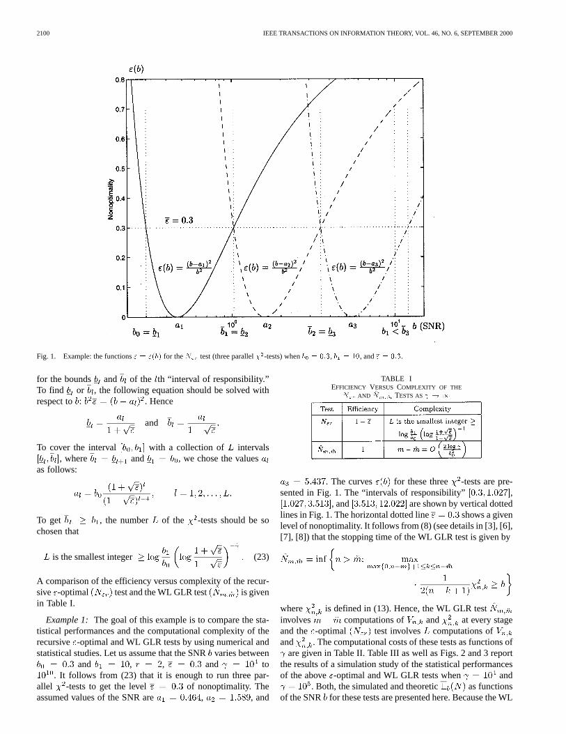
Fig. 1. Example: the functions" = "(b) for theN test (three parallel� -tests) whenb = 0:3, b = 10, and" = 0:3.

for the bounds and of the th “interval of responsibility.”To find or , the following equation should be solved withrespect to : . Hence

and

To cover the interval with a collection of intervals, where and , we chose the values

as follows:

To get , the number of the -tests should be sochosen that

is the smallest integer (23)

A comparison of the efficiency versus complexity of the recur-sive -optimal test and the WL GLR test is givenin Table I.

Example 1: The goal of this example is to compare the sta-tistical performances and the computational complexity of therecursive -optimal and WL GLR tests by using numerical andstatistical studies. Let us assume that the SNRvaries between

and , , and to. It follows from (23) that it is enough to run three par-

allel -tests to get the level of nonoptimality. Theassumed values of the SNR are , , and

TABLE IEFFICIENCY VERSUS COMPLEXITY OF THE

N AND N̂ TESTS AS ! 1

. The curves for these three -tests are pre-sented in Fig. 1. The “intervals of responsibility” ,

, and are shown by vertical dottedlines in Fig. 1. The horizontal dotted line shows a givenlevel of nonoptimality. It follows from (8) (see details in [3], [6],[7], [8]) that the stopping time of the WL GLR test is given by

where is defined in (13). Hence, the WL GLR testinvolves computations of and at every stageand the -optimal test involves computations ofand . The computational costs of these tests as functions of

are given in Table II. Table III as well as Figs. 2 and 3 reportthe results of a simulation study of the statistical performancesof the above -optimal and WL GLR tests when and

. Both, the simulated and theoretic as functionsof the SNR for these tests are presented here. Because the WL


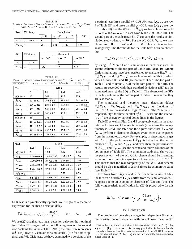
TABLE IIEXAMPLE: EFFICIENCY VERSUSCOMPLEXITY OF THEN AND N̂ TESTS

WHEN b = 0:3, b = 10, " = 0:3, AND = 10 TO 10

TABLE IIIEXAMPLE: MONTE CARLO SIMULATIONS OF THE ~N , N̂ , AND N̂

TESTS WHENb = 0:3, b = 10, r = 2, " = 0:3, AND = 10 OR = 10

GLR test is asymptotically optimal, we use (6) as a theoreticexpression for the mean detection delay

as (24)

We use (22) as a theoretic mean detection delay for the-optimaltest. Table III is organized in the following manner: the secondrow contains the values of the SNR; the third row represents

; rows 4–7 contain the simulated for both -op-timal and WL GLR tests. We have examined two versions of the

-optimal test: three parallel -CUSUM tests ( , see row4 of Table III) and three parallel -GLR tests ( , see row5 of Table III). For the WL GLR we have chosen ;

and 3 (see rows 6 and 7 of Table III). Thesecond part of the table (rows 8–12) contains the results of sim-ulation study when . For the WL GLR we havechosen ; and . This part is organizedanalogously. The thresholds for the tests have been so chosenthat

by using Monte Carlo simulations in each case (see thesecond column of the top part of Table III). Next, MonteCarlo simulations have been performed to evaluate ,

, and for each value of the SNRwhichvaries between and (see columns 3–5 of the top part ofTable III and columns 2–5 of the bottom part of Table III). Theresults are recorded with their standard deviations (SD) (as thesimulated mean the SD) in Table III. The absence of the SDsin the last column of the bottom part of Table III means that theyare less than .

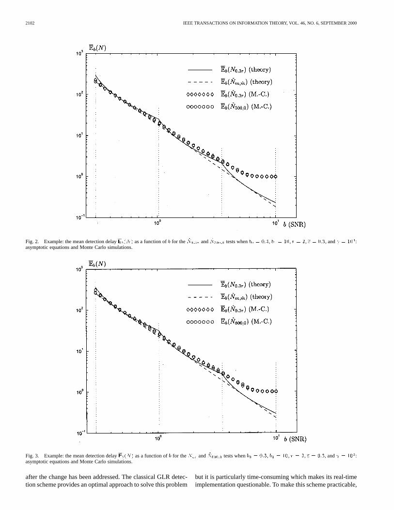
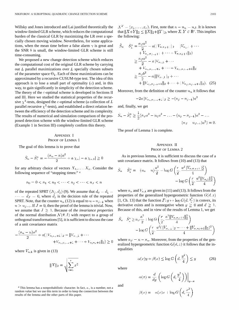
The simulated and theoretic mean detection delays, and as functions of

the SNR are presented in Figs. 2 and 3. The “intervals ofresponsibility” for three parallel -GLR tests and the interval

are shown by vertical dotted lines in the figures.Table III as well as Figs. 2 and 3 completely confirm the theo-

retic performances of the-optimal rule (in our case the nonop-timality is 30%). The table and the figures show that and

perform in detecting changes even better than expectedfrom the asymptotic theory. For example, in detecting changeswith the performance of is better than the perfor-mances of and , and even than the performancesof and (see the second and fourth columns of thebottom part of Table III). The simulation study also shows thatthe parameter of the WL GLR scheme should be magnifiedto two or three times its asymptotic choice when .This means that the real complexity of the WL GLR schemeshould be also magnified to 2 or 3 times its asymptotic value(see Table II).

It follows from Figs. 2 and 3 that for large values of SNRthe theoretic functions differ from the simulated ones. Ithappens due to an asymptotic character of (22) and (24). Thefollowing heuristic modification for (22) is proposed to fix thisgap:

IV. CONCLUSION

The problem of detecting changes in independent Gaussianmultivariate random sequence with an unknown mean vector

3As we have mentioned in Section I, the asymptotic choicem butlogm = o(log ) as ! 1 is not very practicable. To be sure that thecomparison is correct, we first make the simulation of the WL GLR test whenm is the smallest integer> log =b and next we repeat the simulation with abigger value ofm.


Fig. 2. Example: the mean detection delay(N) as a function ofb for theN̂ andN̂ tests whenb = 0:3, b = 10, r = 2, " = 0:3, and = 10 :asymptotic equations and Monte Carlo simulations.

Fig. 3. Example: the mean detection delay(N) as a function ofb for the ~N andN̂ tests whenb = 0:3, b = 10, r = 2, " = 0:3, and = 10 :asymptotic equations and Monte Carlo simulations.

after the change has been addressed. The classical GLR detec-tion scheme provides an optimal approach to solve this problem

but it is particularly time-consuming which makes its real-timeimplementation questionable. To make this scheme practicable,


Willsky and Jones introduced and Lai justified theoretically thewindow-limited GLR scheme, which reduces the computationalburden of the classical GLR by maximizing the LR over a spe-cially chosen moving window. Nevertheless, for some applica-tions, when the mean time before a false alarmis great andthe SNR is small, the window-limited GLR scheme is stilltime-consuming.

We proposed a new change detection scheme which reducesthe computational cost of the original GLR scheme by carryingout parallel maximizations over specially chosen subsetsof the parameter space . Each of these maximizations can beapproximated by a recursive CUSUM-type test. The idea of thisapproach is to lose a small part of optimality () and, in thisway, to gain significantly in simplicity of the detection scheme.The theory of the -optimal scheme is developed in Sections IIand III. Here we studied the statistical properties of the recur-sive -tests, designed the-optimal scheme (a collection ofparallel recursive -tests), and established a direct relation be-tween the efficiency of the detection scheme and its complexity.The results of numerical and simulation comparison of the pro-posed detection scheme with the window-limited GLR scheme(Example 1 in Section III) completely confirm this theory.

APPENDIX IPROOF OFLEMMA 1

The goal of this lemma is to prove that

for any arbitrary choice of vectors . Consider thefollowing sequence of “stopping times:”4

of the repeated SPRT (9). We assume that, where is the decision rule of the repeated

SPRT. Note, that the counter (12) is equal to when. If , then the proof of the lemma is trivial. Now,

we assume that . Because ofthe invariance propertiesof the normal distribution with respect to a group oforthogonal transformations [5], it is sufficient to discuss the caseof a unit covariance matrix

where is given in (13)

4 This lemma has a nonprobabilistic character. In fact,n is a number, not arandom value but we use this term in order to keep the connection between theresults of the lemma and the other parts of this paper.

. First, note that . It is knownthat , where . This impliesthe following:

(25)

Moreover, from the definition of the counter it follows that

and, finally, we get

The proof of Lemma 1 is complete.

APPENDIX IIPROOF OFLEMMA 2

As in previous lemma, it is sufficient to discuss the case of aunit covariance matrix. It follows from (10) and (13) that

where and are given in (11) and (13). It follows from theproperties of the generalized hypergeometric function[1, Ch. 13] that the function is convex, itsderivative exists and is nonnegative when and .Because of this, and in view of the results of Lemma 1, we get

where . Moreover, from the properties of the gen-eralized hypergeometric function it follows that the in-equalities

(26)

where

and


hold for any . In this inequality plays the role of atuning parameter. Therefore, we get

From Lemma 1 it follows that

where the last inequality follows from . Taking intoaccount the equation ,where is a confluent hypergeometric function [1], weget the following asymptotic equations for :

and

as

The proof of Lemma 2 is complete.

APPENDIX IIIPROOF OFLEMMA 3

Let us prove (15) for the recursive -GLR test. Becauseof the invariance propertiesof the normal distributionwith respect to a group of orthogonal transformations, it is suf-ficient to discuss the case of a unit covariance matrix. Hence,the observations are distributed byand are distributed by , where

In this case the decision function (12) is given by

Let us define the following stopping time:

We denote by the largest before the change time. When the change occurs at the

instant , the last cycle of the repeated SPRT can contain someobservations distributed by (a “tail” of prior changeobservations). The integer random valuewill denote the number of such observations. It follows fromLemma 1 that for any arbitrary choice of the vectors

. By applying this inequality to cycle ofthe repeated SPRT we get . Therefore, our plan isthe following: first, we show that as

, where

second, we conclude from the previous result. Wedefine the following fraction:

where , ,, , and if . From [4]

it follows that, if w. p. asunder the distribution , and also, for some , the“large-deviation” probability satisfies

and then

Let us show that w. p. and

w. p. when for a given . To prove the convergence w.p. is equivalent to prove that

as

It is obvious that

It follows from Lemma 4 that . By using Markovinequality, we get

as

We prove now that w. p. , where. The random value is independent of the vec-

tors . We consider the sequence . It fol-lows from [18, Ch. I] that

and

Therefore,

and, in view of Lemma 4,


Hence, the above convergence follows immediately fromMarkov inequality. It follows from the strong law of largenumbers that w. p. . Then, by thecontinuity theorem [5], we get

w. p. . Hence, w. p. under thedistribution .

Now we have to compute the probability

where . It is obvious that

where , , ,, and . It follows from Markov inequality that

It is obvious that

where , , ,, and . Because , where, let us choose . There are two

cases: i) if then

and ii) if then

where , and are twopositive constants. By using the Markov inequality, we get

where, in view of Lemma 4, . It follows from Cher-noff’s theorem [18, Ch. IV] that

where the function , (called theCramér transform)is positive for all . Hence, we get the following inequality:

and, finally, we obtain

This means that starting from somethe probability can beconstrained in the following manner: forand, moreover,

It then follows that and . There-fore, we have shown that and, hence

Because these results are valid for any, follows.Let us discuss the case of the recursive-CUSUM test. From

Lemma 2 it follows that

where and as .Let be as . The rest of the proof of(15) for the -CUSUM test is quite analogous to the case of

-GLR.

APPENDIX IVPROOF OFLEMMA 4

We first prove for the recursive -GLR test. Itfollows from the definition of the nonnegative integer randomvalue that

Hence

Let us compute the probability

It is obvious that


where is distributed according to the central law with de-grees of freedom. From [20] it follows that ,where and are constants, as . Therefore,we get

for any given and finite integer . Let us provefor the recursive -CUSUM test. It follows from

(26) and Lemma 2, that . Hence, ,it then follows that for the recursive -CUSUMtest.

APPENDIX VPROOF OFLEMMA 5

We first prove . Let us define thenonrecursive -CUSUM test

where is the weighted LR (13). It follows from [3] that. It is easily shown that

and, therefore, . It then followsthat

The proof of the first part of the lemma is complete.We next prove

as

Let us define the SNR and the following stoppingtime:

( if no such exists), where

Combining this with the left-hand side of inequality (26) we get

where

From [3] it follows that

where

Hence

Let us choose the parameter as . Since ,, and as , we get

as

The rest of the proof is similar to the first part of the lemma.

APPENDIX VIPROOF OFLEMMA 6

Let us define thenonrecursive change detection rule

where is the weighted (13) or generalized(14) LR. It follows from [9] that the stopping time

can be expressed in the following manner:

where

Hence, the stopping time of the nonrecursive-optimal schemeis

Let us assume that . Therefore,

for any . It follows from [9] that the mean time beforea false alarm is given by . Let us discuss nowthe recursive -optimal scheme . Itis easily shown that and,therefore, . Since

it then follows that

The first inequality (21) follows immediately from

(see [3, Ch. 7]). The second inequality follows from

as (see Lemma 5).

REFERENCES

[1] M. Abramowitz and I. A. Stegun,Handbook of Mathematical Functionswith Formulas, Graphs, and Mathematical Tables, ser. Applied Mathe-matics 55. Washington, DC: U. S. Dept. Commerce, Nat. Bur. Stand.,1964.

[2] M. Basseville, “Information criteria for residual generation and fault de-tection and isolation,”Automatica, vol. 33, no. 5, pp. 783–803, 1997.

[3] M. Basseville and I. V. Nikiforov,Detection of Abrupt Changes. Theoryand Applications, ser. Information and System Sciences. EnglewoodCliffs, NJ: Prentice Hall, 1993.

[4] R. H. Berk, “Some asymptotic aspects of sequential analysis,”Ann.Statist., vol. 1, no. 6, pp. 1126–1138, 1973.


[5] A. A. Borovkov,Theory of Mathematical Statistics—Estimation and Hy-potheses Testing. Moscow, USSR: Nauka, 1984.

[6] T. L. Lai, “Sequential changepoint detection in quality control and dy-namical systems,”J. Roy. Statist. Soc. B, vol. 57, no. 4, pp. 613–658,1995.

[7] T. L. Lai, “Information bounds and quick detection of parameterchanges in stochastic systems,”IEEE Trans. Inform. Theory, vol. 44,pp. 2917–2929, Nov. 1998.

[8] T. L. Lai and J. Z. Shan, “Efficient recursive algorithms for detection forabrupts changes in signals and control systems,”IEEE Trans. Automat.Contr., vol. 44, pp. 952–966, May 1999.

[9] G. Lorden, “Procedures for reacting to a change in distribution,”Ann.Math. Statist., vol. 42, pp. 1897–1908, 1971.

[10] G. Lorden, “Open-ended tsts for Koopman-Darmois families,”Ann.Statist., vol. 1, pp. 633–643, 1973.

[11] G. Moustakides, “Optimal procedures for detecting changes in distribu-tions,” Ann. Statist., vol. 14, pp. 1379–1387, 1986.

[12] I. V. Nikiforov, “Modification and analysis of the cumulative sum pro-cedure,”Automat. Telemekh. (Automat. Remote Contr.), vol. 41, no. 9,pt. 1, pp. 1247–1252, 1980.

[13] I. V. Nikiforov, “On first order optimality of a change detection algo-rithm in a vector case,”Automat. Remote Contr., vol. 55, no. 1, pp.87–105, 1994.

[14] J. J. Pignatiello and G. C. Runger, “Comparisons of multivariateCUSUM charts,”J. Quality Technol., vol. 22, no. 3, pp. 173–186, July1990.

[15] M. Pollak and D. Siegmund, “Approximations to the expected samplesize of certain sequential tests,”Ann. Statist., vol. 3, no. 6, pp.1267–1282, 1975.

[16] M. Pollak, “Optimal detection of a change in distribution,”Ann. Statist.,vol. 13, pp. 206–227, 1985.

[17] Y. Ritov, “Decision theoretic optimality of the CUSUM procedure,”Ann. Statist., vol. 18, pp. 1464–1469, 1990.

[18] A. N. Shiryaev,Probability, ser. Graduate Texts in Mathematics. NewYork: Springer, 1984, vol. 95.

[19] A. S. Willsky and H. L. Jones, “A generalized likelihood ratio approachto detection and estimation of jumps in linear systems,”IEEE Trans.Automat. Contr., vol. AC-21, pp. 108–112, 1976.

[20] M. Woodroofe, “Large deviation of likelihood ratio statistics with ap-plications to sequential testing,”Ann. Statist., vol. 6, no. 1, pp. 72–84,1978.

[21] B. Yakir, “A note on optimal detection of a change in distribution,”Ann.Statist., vol. 25, no. 5, pp. 2117–2126, 1997.

Documents

A suboptimal quadratic change detection scheme