A STUDY ON THE FACTORS AFFECTING THE ECONOMICAL LIFE OF HEAVY CONSTRUCTION EQUIPMENT

Hongqin Fan and Zhigang Jin

Department of Building and Real Estate, The Hong Kong Polytechnic University, Kowloon, Hong Kong

* Corresponding author (bshfan@inet.polyu.edu.hk)

ABSTRACT: Surveys found that large contractors replace approximately 10% of their equipment fleet units annually in

North America. Cost minimization model is a commonly accepted method for equipment replacement which helps to

identify these equipment units whose total owning and operating cost reaches their minimum point as candidates for

replacement. While the model is conceptually clear with the aim of achieving minimum equipment cost per unit of service,

its use has some practical difficulties as the equipment maintenance and repair costs experience bumps and lumps in the its

life time. In practice, identification of equipment units for replacement are still based on such metrics as limit of repair

costs, limit of major failures, lessons learned from previous cases as well as expert knowledge. In this research, we look

into the cost history of a large number of equipment units in a contractor’s equipment management information system

(MIS) and use decision tree modeling approach to identify these factors impacting on the economic life of first hand

equipment, and extract rules leading to different cost patterns and therefore different economic life spans of heavy

equipment. C4.5 decision tree model is used to build a top-down decision tree by recursively splitting existing cases based

on the concept of information gain. In addition to facilitating decisions in equipment replacement, the findings can also be

used to explain the effectiveness of various maintenance strategies, compare the equipment cost performance among

various classes, makes, and amount of services in their life cycle.

Keywords: Construction Equipment, Replacement Analysis, Decision Tree Modeling, Decision Support

1. INTRODUCTION

Heavy construction equipment fleet is a critical resource

for large contractors. To keep competitive in the market,

the contractor needs to identify these candidates of

equipment items for timely replacement. A survey found

that nearly 10% of the equipment needs to be replaced

annually on average in USA [4]. Although there are many

equipment replacement theories, such as cost minimization

models, their practical use is rare as the total annual cost

every equipment item shows significant bumps and lumps,

it is also difficult to model the trend of equipment cost to

define the most likely economical life for a particular type

of equipment under the dynamic influences of multiple

factors.

This paper introduces a machine learning approach to

address the equipment replacement problem. Decision tree

induction algorithm C4.5 proposed by Ross Quinlan [3] is

used to perform inductive learning from the real equipment

cost data. A decision tree model is derived for describing

the rule sets leading to different cost cohorts. Combined

with traditional mathematical and statistical approaches,

the decision tree model can effectively evaluate these

factors of impact on the fluctuation of equipment costs,

and identify the equipment candidates for replacement

based on their cost-related features.

2. LITERATURE REVIEW

S27-1

923

 

 

Cost minimization method, first proposed by Taylor [5], is

one of the earliest approaches for equipment replacement

and is well accepted in academia and construction,

agriculture and forestry industries. This method aims to

minimize the annual owning and operating cost of a piece

of equipment per unit of service: the equipment annual

costs drop sharply in the first few years due to high

depreciation, and rise gradually in the following years

when the equipment repair costs escalate due to equipment

aging, tear and wear. The method relies on various

theoretical cost models to predict the future costs and

identify the point of time at which the annual unit cost

reaches its minimum.

Many mathematical and statistical models are proposed for

practical use in equipment replacement. Collier and

Jacques [1] proposed a “Geometric Gradient-to-Infinite-

Horizon method”, for projecting expected future life-cycle

costs for the existing machine plus future replacements to

an infinite horizon; Vorster and Sears [6] suggested to use

failure cost profiles for consequential costs of equipment

failures and incorporated into the equipment cost model

for equipment replacement. Gillerspie et al. [2] addressed

the equipment replacement in a research project by the

Virginia Transportation Research Council in corporation

with U.S. Department of Transportation, the focus of their

research is on the prediction of annual variable costs of a

piece of equipment using statistical approaches, however

the researcher acknowledged the difficulties in the

inclusion of large number of attributes into the predictor

variables, as well as the tedious trial and error method in

statistical analysis.

3. PROBLEM STATEMENT

A general contractor owns a large fleet of equipment to

satisfy the needs for equipment resources in its civil and

transportation projects. The contractor notices there are

large variations of economic life spans for different types

of equipment; and these variations also exist for the same

class of equipment with different make, preventive

maintenance (PM) history, accumulated unit of services

(hours or kilometers), etc. The current annual equipment

replacement exercise focuses on the metrics of maximum

equipment use and the accumulated repair costs and

personal judgment. The statistical cost information on

equipment groups is useful but not specific enough to

guide the equipment replacement. Replacing a piece of

equipment too early or too late is obviously a problem that

will increase the equipment “internal rate” charged to

projects and decrease the contractor’s competitive edge in

the equipment-intensive heavy construction market.

Take the fleet of dump trucks as an example, the contractor

needs to know what caused the discrepancy between the

manufacturer’s recommended life and the actual life in the

contractor’s fleet, and how the combination of the

influencing factors reduce or increase the equipment life

span. If the impact from these factors can be characterized,

the equipment replacement can be done with more

confidence and less guesswork. The future purchase of

new equipment can also benefit from these findings, for

example, comparison between different makes/models

under specified conditions.

4. DECISION TREE INDUCTION: C4.5 ALGORITHM

Decision tree induction is one category of machine

learning algorithm for building a decision tree structure

linking different decision conditions with different results.

A decision tree is a top-down structure with the root node

at the top, questions are asked with different answers

leading to the next level decision nodes or terminal leaf

nodes. With a tree-like multi-level structure, decision tree

is equivalent to a set of decision questions asked

consecutively and a combination of different

questions/answers lead to different results.

Building decision tree from data is an inductive learning

process, a supervised learning algorithm is used to

repetitively partition the data space into subset of data with

more purer results. One major different between different

decision tree algorithms is how to search for

attribute/value pairs for splitting the data space. C4.5

S27-1

924

 

 

algorithm uses information gain to judge which attribute

and which value to use for data splitting, which is defined

in the following equations:

Entropy: the degree of purity in the dataset, does the

dataset contain pure or ambiguous information on

classification results?

21

( ) logc

i ii

Entropy S p p

………………….[1]

Where pi is the proportion of original dataset S belonging

to Class i, c is the number of classes

Information gain: the amount of information increase in

the dataset after knowing attribute A of dataset S

( )

( , ) ( ) ( )vv

v Values A

SGain S A Entropy S Entropy S

S

……………………………………………………….[2]

Where values (A) is the set of all possible values for

attribute A, Sv is the subset of S for which attribute A has

value v.

Split Information: the amount of information in the

dataset after partitioning by c-valued attribute A

21

logc

i i

i

S SSplitInformation

S S

……….[3]

Where Si ~Sc are the c subsets of examples resulting from

partitioning S by the c-valued attribute A.

Information gain ratio: the ratio between information

gain and split information ( , )

( , )( , )

Gain S AGainRatio S A

SplitInformation S A ….[4]

This gain ratio is used to select criteria for splitting dataset

S into subsets. From the root node, the C4.5 algorithm

scans over the dataset with various splitting options :

different attributes and different splitting values (for

example, a conjunction of the attribute “equipment age”

and value “5” composes a decision question “if the

equipment age is less than 5 years”). The splitting criteria

leading to the largest information gain ratio indicates the

best combination of attribute and splitting values, or the

best partitioning of dataset with subsets containing pure

and consistent information on equipment costs. The same

splitting process is repeated on the subsets of data or child

nodes for further growing of trees down the paths, if the

termination criteria are satisfied (too few number of cases

or sufficiently pure information in the node) and take the

child nodes as leaf nodes in the tree structure, otherwise,

take the child node as a decision node and continue the

splitting process until all the nodes are terminal leaf nodes.

5. MODELING OF THE EQUIPMENT M&R COST USING C4.5 DECISION TREE ALGORITHM

Among all the owning and operating cost items,

maintenance and repair (M&R) costs are the most

uncertain element which is the most difficult to predict.

The M&R costs cover such items as preventive

maintenance, work order repairs (repairs at the shop), and

running repairs (repairs on the shift). The spending is

necessary to keep the equipment running with maintenance

actions and timely repairs. The predictive model on the

annual equipment M&R cost is trained, validated and used

to facilitate equipment replacement analysis.

Data preparation

The M&R cost model is learned from a large collection of

equipment data on a group of 180 units of dump trucks

with capacities of 6 tons and above, with the following

features:

The dump trucks belong to different operational

divisions of the contractor

8 factors of potential impact on equipment M&R

cost are selected and shown in Table 1

The annual M&R costs of these units are

collected for the years 2006-2010 for study

Inclusion of correlated variables tends to overestimate the

contributions from one factor and make the model unstable,

showing phenomena of multicollearity. A simple

correlation analysis found that the AnnualKM and

AnnualFuelCost are highly correlated, with a correlation

factor of 0.89, therefore the Annual fuel volume is

reserved as a more accurate measurement of equipment

S27-1

925

 

 

service as it takes the truck load level and environment

conditions into consideration.

Tab. 1 Attributes for equipment group “Dump trucks, 6

tons and above” Factors of Impact

Nr Predictor Variables Description

1 Age, numerical variable age of the equipment unit, in years

2 Manufacturer, categorical variable

Manufacturer of the equipment unit

4 Division, categorical variable

Operating division of the contractor

5 Class, categorical variable

Class of equipment

6 AnnualPMcost, numerical variable

Annual preventive maintenance cost, in 2006 constant dollars

7 AnnualKM, numerical variable

Annual travelling distance, odometer readings difference from year start to end, in Kilometers

8 AnnualFuelCost, numerical variable

Annual accumulated fuel cost, in 2006 constant dollars

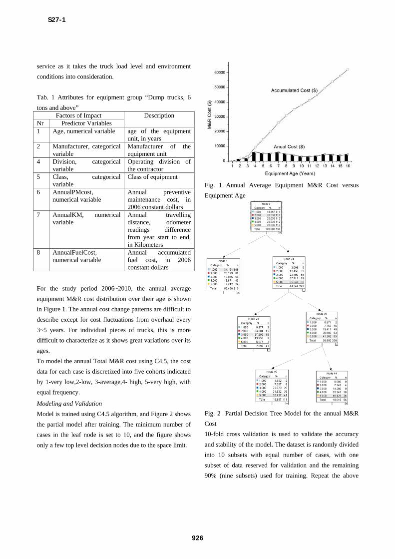
For the study period 2006~2010, the annual average

equipment M&R cost distribution over their age is shown

in Figure 1. The annual cost change patterns are difficult to

describe except for cost fluctuations from overhaul every

3~5 years. For individual pieces of trucks, this is more

difficult to characterize as it shows great variations over its

ages.

To model the annual Total M&R cost using C4.5, the cost

data for each case is discretized into five cohorts indicated

by 1-very low,2-low, 3-average,4- high, 5-very high, with

equal frequency.

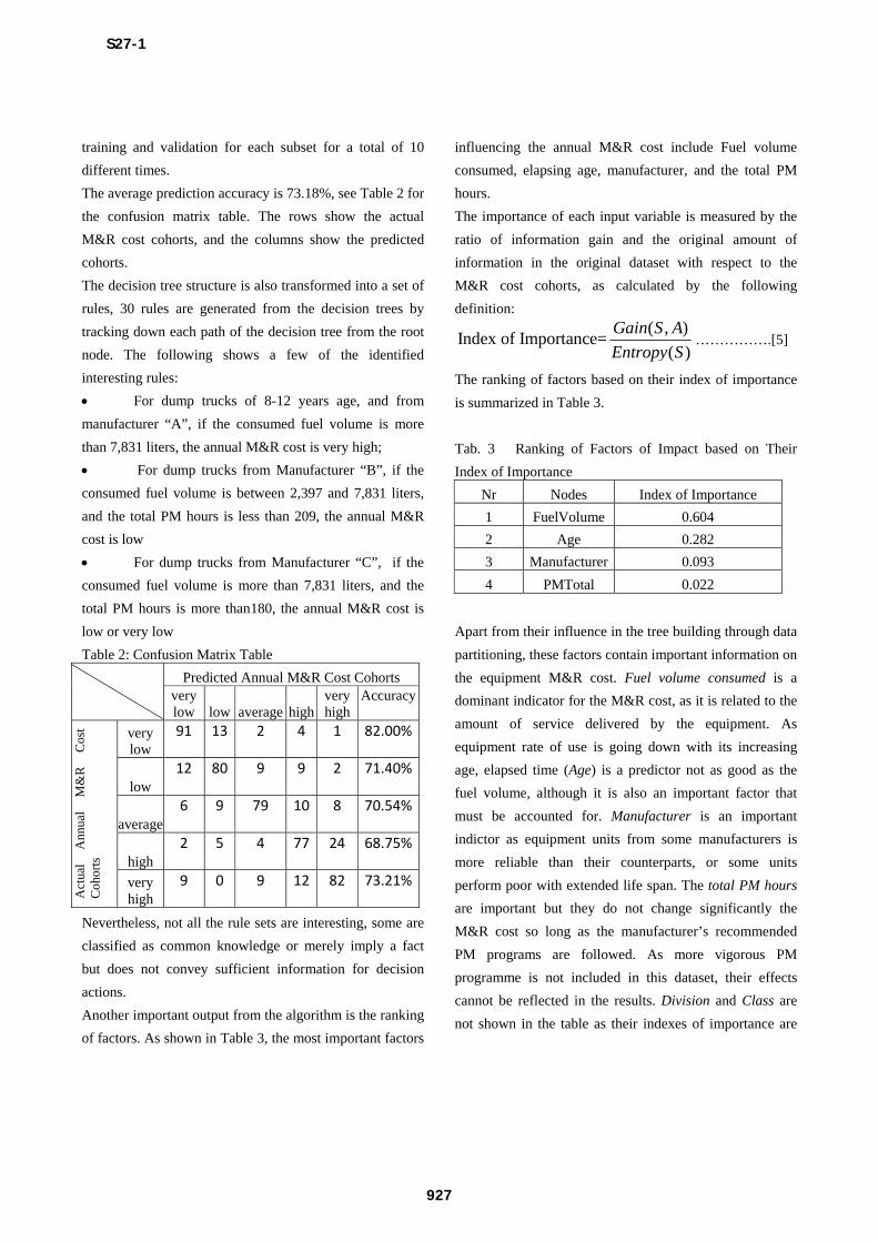
Modeling and Validation

Model is trained using C4.5 algorithm, and Figure 2 shows

the partial model after training. The minimum number of

cases in the leaf node is set to 10, and the figure shows

only a few top level decision nodes due to the space limit.

Fig. 1 Annual Average Equipment M&R Cost versus

Equipment Age

Fig. 2 Partial Decision Tree Model for the annual M&R

Cost

10-fold cross validation is used to validate the accuracy

and stability of the model. The dataset is randomly divided

into 10 subsets with equal number of cases, with one

subset of data reserved for validation and the remaining

90% (nine subsets) used for training. Repeat the above

S27-1

926

 

 

training and validation for each subset for a total of 10

different times.

The average prediction accuracy is 73.18%, see Table 2 for

the confusion matrix table. The rows show the actual

M&R cost cohorts, and the columns show the predicted

cohorts.

The decision tree structure is also transformed into a set of

rules, 30 rules are generated from the decision trees by

tracking down each path of the decision tree from the root

node. The following shows a few of the identified

interesting rules:

For dump trucks of 8-12 years age, and from

manufacturer “A”, if the consumed fuel volume is more

than 7,831 liters, the annual M&R cost is very high;

For dump trucks from Manufacturer “B”, if the

consumed fuel volume is between 2,397 and 7,831 liters,

and the total PM hours is less than 209, the annual M&R

cost is low

For dump trucks from Manufacturer “C”, if the

consumed fuel volume is more than 7,831 liters, and the

total PM hours is more than180, the annual M&R cost is

low or very low

Table 2: Confusion Matrix Table

Predicted Annual M&R Cost Cohorts

very low low average high

very high

Accuracy

very low

91  13  2  4  1  82.00%

low 12  80  9  9  2  71.40%

average 6  9  79  10  8  70.54%

high 2  5  4  77  24  68.75%

Act

ual

Ann

ual

M&

R

Cos

t C

ohor

ts

very high

9  0  9  12  82  73.21%

Nevertheless, not all the rule sets are interesting, some are

classified as common knowledge or merely imply a fact

but does not convey sufficient information for decision

actions.

Another important output from the algorithm is the ranking

of factors. As shown in Table 3, the most important factors

influencing the annual M&R cost include Fuel volume

consumed, elapsing age, manufacturer, and the total PM

hours.

The importance of each input variable is measured by the

ratio of information gain and the original amount of

information in the original dataset with respect to the

M&R cost cohorts, as calculated by the following

definition:

( , )Index of Importance=

( )

Gain S A

Entropy S…………….[5]

The ranking of factors based on their index of importance

is summarized in Table 3.

Tab. 3 Ranking of Factors of Impact based on Their

Index of Importance

Nr Nodes Index of Importance

1 FuelVolume 0.604

2 Age 0.282

3 Manufacturer 0.093

4 PMTotal 0.022

Apart from their influence in the tree building through data

partitioning, these factors contain important information on

the equipment M&R cost. Fuel volume consumed is a

dominant indicator for the M&R cost, as it is related to the

amount of service delivered by the equipment. As

equipment rate of use is going down with its increasing

age, elapsed time (Age) is a predictor not as good as the

fuel volume, although it is also an important factor that

must be accounted for. Manufacturer is an important

indictor as equipment units from some manufacturers is

more reliable than their counterparts, or some units

perform poor with extended life span. The total PM hours

are important but they do not change significantly the

M&R cost so long as the manufacturer’s recommended

PM programs are followed. As more vigorous PM

programme is not included in this dataset, their effects

cannot be reflected in the results. Division and Class are

not shown in the table as their indexes of importance are

S27-1

927

 

 

close to zero, showing they do not have any impact on the

equipment cost fluctuations.

6. DISCUSSIONS ON THE M&R COST MODEL

The derived M&R cost model is very useful for

discovering interesting rules for equipment replacement

decision support as the rule sets quantify the effects on

cost change patterns caused by the various factors of

impact. These inherent rules are difficult to identify by

domain experts.

The identified rules can help to conduct the equipment

replacement analysis on a particular piece of equipment.

For a particular piece of equipment, identified rules can

help the decision maker to predict the equipment M&R

cost level in the coming years. Although it is not possible

to predict the future M&R cost with a very high accuracy,

the model can incorporate the influencing factors and

improve the prediction results with significant

improvement.

Other typical use of identified interesting rules sets include:

comparison of equipment cost performance among

manufacturers during the expected life span; comparison

of equipment PM strategies by evaluating if improved PM

frequencies really could help to reduce the equipment

repair costs for a certain group of equipment.

The most interesting rules identified are these on the

lowest cohort (1) and these on the highest cohort (5) of the

annual M&R cost. By contrasting these combined

conditions leading to the most desirable and the worst case

scenarios, the decision makers can learn lessons and

improve their practice in equipment maintenance

management.

7. CONCLUSIONS

The paper summarizes our research on the descriptive and

predictive analysis of equipment M&R cost and its

influencing factors using C4.5 decision Tree induction

algorithm. Decision rules can be generated from the

existing equipment data for decision support in equipment

replacement. Factors of impact on the variations of

equipment M&R cost are identified, prioritized, and used

for decision analysis. The research supplements the

traditional equipment replacement theory by combining

the fact-based cost-related rules into the traditional

equipment replacement models, reducing the uncertainties

and hypothesis involved in practical applications.

8. ACKNOWLEDGMENT

The research is supported by the General Research Fund

(GRF) Nr. 517009 of Research Grant Council, Hong Kong

SAR, China

REFERENCES

[1] Collier, C. A. and Jacques, D. E., “Optimum

Equipment Life by minimum Life-cycle Costs”,

Journal of Construction Engineering and Management,

ASCE, Vol. 110, No. 2, pp.248-265, 1984

[2] Gillerspie, J.S. and Hyde A. S., The

replacement/repair decision for heavy equipment,

Report VTRC 05-R8, Virginia Transportation

Research Council, November 2004.

[3] Quinlan, J. R., C4.5: Programs for Machine

Learning. Morgan Kaufmann Publishers, Mateo, CA.,

1993

[4] Reed Business Information, Annual Report and

Forecast. Supplement to Construction Equipment,

January 2007 issue, New York, NY.

[5] Taylor, J. S., “A Statistical Theory of

Depreciation Based on Units Cost”, Journal of the

American Statistical Association, pp.1010-1023, 1923

[6] Vorster, M.C. and Sears, G.A., “Model for

Retiring, Replacing, or Reassigning Construction

Equipment”, Journal of Construction Engineering and

Management, ASCE, Vol. 113(1), pp.125-137, 1987

S27-1

928