A STUDY ON SOLUTION OF DIFFERENTIAL EQUATIONS USING

HAAR WAVELET COLLOCATION METHOD

A PROJECT REPORT SUBMITTED IN FULLFILLMENT OF THE REQUIREMENTS OF

THE DEGREE OF

MASTER OF SCIENCE

IN

MATHEMATICS

SUBMITTED TO

NATIONAL INSTITUTE OF TECHNOLOGY, ROURKELA

BY

BISHNUPRIYA SAHOO

ROLL NUMBER 410MA2103

UNDER THE SUPERVISION OF

PROF. SANTANU SAHA RAY

DEPARTMENT OF MATHEMATICS

NATIONAL INSTITUTE OF TECHNOLOGY

ROURKELA-769008

NATIONAL INSTITUTE OF TECHNOLOGY

ROURKELA

DECLARATION

I hereby certify that the work which is being presented in the thesis entitled “A study

on solution of differential equations using Haar wavelet collocation method” in partial

fulfilment for the award of degree of Master of Science, submitted in the Department of

Mathematics, National Institute of Technology, Rourkela is an authentic record of my own

work carried out under the supervision of Prof. S. Saha Ray. The matter embedded in this

thesis has not been submitted by me for the award of any other degree.

Bishnupriya sahoo

Roll No. 410MA2103

Department of Mathematics

NIT, Rourkela

NATIONAL INSTITUTE OF TECHNOLOGY

ROURKELA

CERTIFICATE

This is to certify that the above declaration made by the candidate is correct to the

best of my knowledge.

Prof. Santanu Saha Ray

National Institute of Technology

Rourkela-769008

Odisha, India

NATIONAL INSTITUTE OF TECHNOLOGY

ROURKELA

ACKNOWLEDGEMENT

With immense pleasure I wish to express my profound sense of reverence and

gratitude to Prof. S. Saha Ray for the encouragement, constructive guidance and thought-

provoking discussions throughout the period of my project work, which enabled me to

complete the project report so smoothly.

Words at my command are inadequate to convey my profound to my parents whose

love, affection and blessings and the support and love of my sisters and friends has inspired

me the most.

Bishnupriya sahoo

Roll No. 410MA2103

Department of Mathematics

NIT, Rourkela

ABSTRACT

In this contest of study, problems regarding differential equations are studied when

the differential equations: ordinary or partial differential equations have no solution in direct

method or it is very difficult to find the required integral.

When this type of problem arises, mainly numerical solution method comes to a

picture. From the different numerical methods haar wavelet transform method is one to use it

in solving differential equations.

Before coming directly to the solution of differential equations haar wavelet function

and its properties are studied. Using the properties of haar wavelet transform a useful term

from the differential equation is approximated by the summation of constant multiples of the

haar functions which are known functions and easy to handle. Then the other terms of the

differential equations are found out by integrating or differentiating the above discussed

problem.

Using a logical method the differential equations are solved. And it is observed that

the solution gives less error. So this method can be an efficient method.

CONTENTS Page No.

1. Introduction 1

2. Haar Wavelet and its Properties 2

3. Solution Method of Ordinary Differential

Equations (Initial Value Problems) and examples 7

4. Solution Method of Ordinary Differential

Equations (Boundary Value Problems) and examples 9

5. Solution Methods of Partial Differential Equations

with examples 15

6. Conclusion 22

7. References 23

1

1. Introduction:

Numerical Analysis starts with the difficulties in finding the solution of an equation in

a direct method or in a theoretical method proposed earlier to find the exact solution. In case

of complicacy in finding the solution numerical methods with respectively lesser error are

proposed.

We know the methods like Bisection method, Secant method, Newton Raphson

method to find the root of an equation. But when the equation includes a differential operator

i.e. a differential equation the known numerical solution methods are Picards method, Rungee

kutta method etc.

For a better solution i.e. for an approximated solution with lesser error we use various

collocation methods. As there is no direct method to solve type of equations like Van-Der-Pol

equation and Fisher’s equation, hence for the solution, a numerical method can be used.

Here in this contest of study, HAAR Wavelet Transform Method to find the solution

of typical differential equations like Van-Der-Pol equation and Fisher’s equation. The idea of

Wavelets can be summarised as a family of functions constructed from transformation and

dilation of a single function called mother wavelet. From various type of continuous and

discrete wavelets HAAR Wavelet is the discrete type of wavelet which was 1st proposed and

the 1st orthonormal wavelet basis is the Haar basis.

2

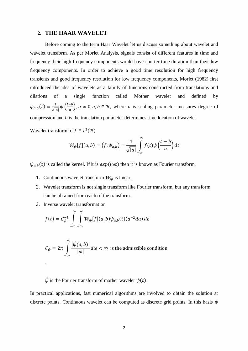
2. THE HAAR WAVELET

Before coming to the term Haar Wavelet let us discuss something about wavelet and

wavelet transform. As per Morlet Analysis, signals consist of different features in time and

frequency their high frequency components would have shorter time duration than their low

frequency components. In order to achieve a good time resolution for high frequency

transients and good frequency resolution for low frequency components, Morlet (1982) first

introduced the idea of wavelets as a family of functions constructed from translations and

dilations of a single function called Mother wavelet and defined by

, where a is scaling parameter measures degree of

compression and b is the translation parameter determines time location of wavelet.

Wavelet transform of

is called the kernel. If it is then it is known as Fourier transform.

1. Continuous wavelet transform is linear.

2. Wavelet transform is not single transform like Fourier transform, but any transform

can be obtained from each of the transform.

3. Inverse wavelet transformation

.

is the Fourier transform of mother wavelet

In practical applications, fast numerical algorithms are involved to obtain the solution at

discrete points. Continuous wavelet can be computed as discrete grid points. In this basis

3

can be defined

replacing a by

and b by

Then the wavelet transform

- Discrete wavelet or simple wavelet.

In general can be completely determined by its discrete wavelet transform

if the wavelets form a complete system in . Otherwise, if the wavelets form an

orthonormal basis then they are complete.

, provided the wavelets form an orthonormal basis.

With the choice , there exists a function with good time frequency

localisation properties such that

constitute an orthonormal

basis for is the Haar Wavelet.

Precisely,

and the Haar basis is called the 1st orthonormal basis.

4

PROPERTIES OF HAAR WAVELET:

1. Haar wavelet is very well localised in the time domain, but not continuous.

2.

and

3. Any continuous real function can be approximated by linear combination of Φ(t),

Φ(2t), Φ(4t),... , Φ(2k t),... and their shifted functions.

This extends the function space where any function can be approximated by

continuous functions.

4. Any continuous real function can be approximated by linear combination of the

constant functions and their shifted functions.

5. Each two Haar function is orthogonal to each other i.e.

6. Wavelet function or scaling function with different scale m have a functional

relationship Φ(t)= Φ(2t)+ Φ(2t-1) and = Φ(2t)- Φ(2t-1).

Practical Application of Haar Wavelet:

Its practical use is in photography or more specifically construction of high resolution

camera. We know that if the pixel rate of camera is high then it is a good one. This pixel

word comes from the term point. In this case small squares are assumed as points and

Haar wavelet is defined in it. The smaller square size gives rise to more resolution and a

better quality picture.

5

Haar Wavelets and Integration of Haar Wavelets:

The Haar Wavelet family for is defined by

where j indicates the level of

wavelet, k denotes translation parameter and J denotes the maximum level of resolution.

The index is determined by where the minimum values of k and

m are 0 and 1 respectively.

The maximum value of

The introduced notations are as follows

In particular when i=1

Else

6

The Method of Solution:

Form the property of the Haar wavelet Transformation, which is a function of x can be

approximated by the Haar Wavelet function like wise

To get the solution , it is difficult to find if the Differential Equation is nonlinear type or

complicated to integrate .

But approximating the with Haar wavelet function it is quite easier to have

explicitly in terms of x.

i.e.

and

7

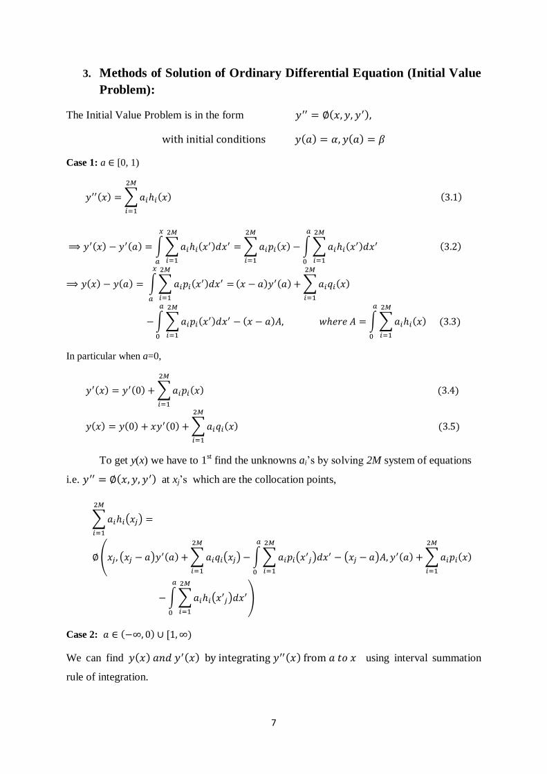
3. Methods of Solution of Ordinary Differential Equation (Initial Value

Problem):

The Initial Value Problem is in the form

Case 1: a [0, 1)

In particular when a=0,

To get y(x) we have to 1st find the unknowns ai’s by solving 2M system of equations

i.e. at xj’s which are the collocation points,

Case 2:

We can find using interval summation

rule of integration.

8

Example: 3.1

Solution of Van Der Pol Equation

The exact solution is

Table 3.1

The comparison of exact solution and Haar Solution of Van-Der-Pol Equation:

x Exact Solution Haar Solution Error

0 1 1 0

0.125 0.992198 0.99224 0.0000425132

0.375 0.930508 0.930632 0.000124536

0.625 0.810963 0.81117 0.000206634

0.875 0.640997 0.641235 0.000238164

Exact solution

….. Approximate solution

[Fig 3.1 Comparison of exact solution and Haar solution of Van-Der-Pol Equation]

0.2 0.4 0.6 0.8x

0.70

0.75

0.80

0.85

0.90

0.95

1.00

u x

9

4. Methods of Solution of Ordinary Differential Equation (Boundary

Value Problem):

Case 1:

From (4.1.3) and (4.1.4) we have

Hence the corresponding approximations are

Solving above system of equations for unknowns y (0) and ai, at i≠1, approximate solution

y(x) in (4.1.7) can be found out.

10

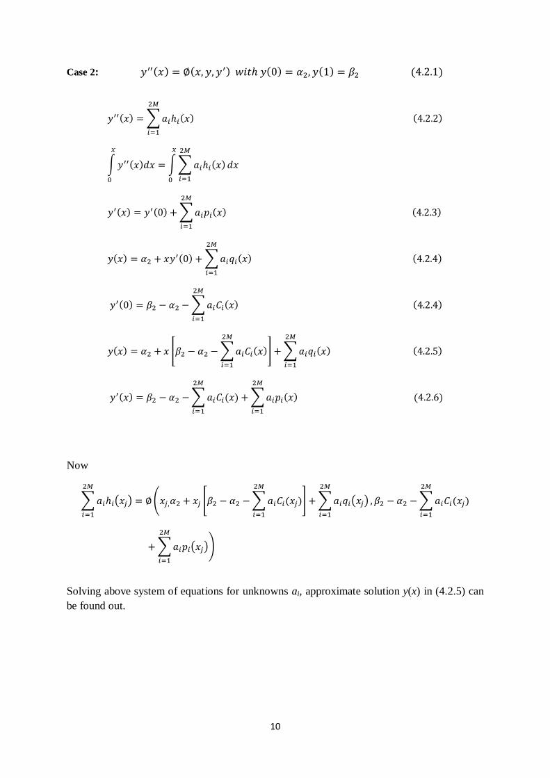
Case 2:

Now

Solving above system of equations for unknowns ai, approximate solution y(x) in (4.2.5) can

be found out.

11

Case 3:

Solving above system of equations for unknowns ai, approximate solution y(x) in (4.3.4) can be found

out.

Case 4:

12

Solving above system of equations for unknowns ai, approximate solution y(x) in (4.4.4) can

be found out.

Case 5:

Solving above system of equations for unknowns ai, approximate solution y(x) in (4.5.6) can

be found out.

13

Example 4.1

The exact solution is

This is a BVP of case 2 discussed above.

Table 4.1

The comparison of exact solution and Haar Solution of

x 1/(1+x) Haar y(x) Error

0 1 0.934012 0.0659877

0.125 0.888889 0.81755 0.0713384

0.375 0.727273 0.631248 0.0960249

0.625 0.615385 0.486979 0.128406

0.875 0.533333 0.407181 0.126152

Exact solution

….. Approximate solution

[Fig 4.1 Comparison of exact solution and Haar solution of ]

0.2 0.4 0.6 0.8 1.0x

0.5

0.6

0.7

0.8

0.9

1.0

y x

14

Example 4.2

The exact solution is

This is a Boundary Value Problem of Case 2 discussed above.

Table 4.1

The comparison of exact solution and Haar Solution

x Cos x Haar y(x) Error

0 1 1 0

0.125 0.992198 0.995543 0.00334484

0.375 0.930508 0.938405 0.00789711

0.625 0.810963 0.821593 0.0106297

0.875 0.640997 0.653346 0.123487

Exact solution

….. Approximate solution

[Fig 4.2 Comparison of exact solution and Haar solution]

0.2 0.4 0.6 0.8x

0.70

0.75

0.80

0.85

0.90

0.95

1.00

y x

15

5. Method to solve Partial Differential Equation:

Example 5.1 (Solution Method of Sine-Gordon Equation)

Let us assume the Partial Differential Equation with two independent variables. For example

let it be Sine-Gordon equation i.e.

where u= is a function of x and t , (x,t) are discrete points in the form where

Keeping in view with the initial and boundary conditions we have to approximate

The following steps show the clear view of logic behind the approximated solution method.

Let us consider, the Partial Differential Equation

with the initial and boundary conditions

Step1: We approximate

Step 2: We integrate above once and twice w.r.t. from 0 to and w.r.t. from to we get

16

Step 3: The approximated values (5.1.3) in step 2 are substituted in equation (5.1.1) in step 1.

At t=ts+1 solving the system of equations (5.1.1) generated by 2M collocation points for

unknowns as(i)’s, the approximate solution u(x,t) in (5.1.3) can be found out.

Clearly these as(i)’s are only valid for the range

Step 4: Initially =0 and

After 1st iteration are obtained which are treated as the boundary

condition and initial condition instead of and can

be found out following the previous steps.

Proceeding likewise we will have the set of solutions at different . Hence we

get a two dimensional solution treating each iteration as one dimensional problem.

Example 5.2 (Numerical Solution Method of Fisher’s Equation)

Fisher’s Equation:

With initial and boundary conditions

(5.2.2)

Let us approximate

17

(5.2.3)

So,

At t=ts+1 solving the system of equations (5.2.4) generated by 2M collocation points for

unknowns as(i)’s, the approximate solution u(x,t) in (5.2.3) can be found out when

.

The exact solution of the given Fisher’s equation is

The solution is brought out by using MATHEMATICA.The comparison of approximate Haar solution

and exact solution is cited in the tables below.

Table 5.2.1

18

t x=0

u(x,t) Exact Error

0.0 0.25 0.25 0

0.1 0.387456 0.387456 0

0.2 0.534447 0.534447 0

0.3 0.668428 0.668428 0

0.4 0.77580 0.77580 0

0.5 0.854038 0.854038 0

0.6 0.907397 0.907397 0

0.7 0.942235 0.942235 0

0.8 0.964351 0.964351 0

0.9 0.978147 0.978147 0

1.0 0.986659 0.986659 0

Table 5.2.2

t x=0.125

u(x,t) exact Error

0.0 0.219765 0.219765 0

0.1 0.331601 0.351254 0.0196532

0.2 0.477158 0.498133 0.0209742

0.3 0.618858 0.637102 0.0182438

0.4 0.73778 0.751751 0.0139708

0.5 0.827364 0.837044 0.00967978

0.6 0.889889 0.896045 0.00615616

0.7 0.931341 0.934923 0.0035815

0.8 0.957919 0.959749 0.00183003

0.9 0.974601 0.975291 0.000690132

1.0 0.984935 0.984903 0.0000317345

Table 5.2.3

19

t x=0.375

u(x,t) exact Error

0.0 0.16592 0.16592 0

0.1 0.121348 0.282183 0.160836

0.2 0.241005 0.424263 0.183258

0.3 0.40585 0.569897 0.164047

0.4 0.569473 0.698033 0.12856

0.5 0.707203 0.798002 0.0907986

0.6 0.810899 0.869469 0.0585698

0.7 0.883233 0.917596 0.034363

0.8 0.931182 0.948759 0.0175776

0.9 0.961928 0.96844 0.00651222

1.0 0.981231 0.980677 0.000553802

Table 5.2.4

t x=0.625

u(x,t) exact Error

0.0 0.121553 0.121553 0

0.1 -0.102173 0.219765 0.321938

0.2 -0.0989373 0.351254 0.450191

0.3 0.054176 0.498133 0.443956

0.4 0.261209 0.637102 0.375893

0.5 0.468066 0.751751 0.283685

0.6 0.643754 0.837044 0.193289

0.7 0.777303 0.896045 0.118742

0.8 0.871258 0.934923 0.0636648

0.9 0.933956 0.959749 0.0257925

1.0 0.974354 0.975291 0.00093736

Table 5.2.5

20

t x=0.875

u(x,t) Exact Error

0.0 0.0865624 0.0865624 0

0.1 -0.176485 0.16592 0.342406

0.2 -0.361698 0.282183 0.643882

0.3 -0.330027 0.424263 0.75429

0.4 -0.158322 0.569897 0.728218

0.5 0.082333 0.698033 0.6157

0.6 0.335699 0.798002 0.462303

0.7 0.560501 0.869469 0.308968

0.8 0.737147 0.917596 0.180449

0.9 0.864426 0.948759 0.0843328

1.0 0.950774 0.96844 0.0176659

21

Exact solution

….. Approximate solution

[Fig 5.2.1 Plot of exact and approximate solution of Fisher’s equation at x=0]

[Fig 5.2.2 Plot of exact and approximate solution of Fisher’s equation at x=0.125]

[Fig 5.2.3 Plot of exact and approximate solution of Fisher’s equation at x=0.375]

0.0 0.2 0.4 0.6 0.8 1.0t

0.2

0.4

0.6

0.8

1.0

u x,t

0.0 0.2 0.4 0.6 0.8 1.0t

0.2

0.4

0.6

0.8

1.0

u x,t

0.0 0.2 0.4 0.6 0.8 1.0t

0.2

0.4

0.6

0.8

1.0

u x,t

22

6. Conclusion

1. Haar Wavelet transform method is best shoot for the initial value problems, boundary value

problems as well as the partial differential equations with less error.

2. It is easy to get solution in two dimensions so it is better over all other methods.

3. It is observed that if the level of resolution is more i.e. if the collocation points are more then

we can get a better solution with lesser error.

4. Like Fisher’s equation or Sine Gordon equation we can solve all non linear type critical partial

differential equations.

5. One of the drawbacks is that to find the constants we solve linear or nonlinear equations which

may impossible without mathematical software.

6. Simply availability and fast convergence of the Haar wavelets provide a solid foundation for

highly nonlinear problems of differential equations.

7. These discussed method with far less degrees of freedom and small computation time provides

better solution.

8. It can be concluded that this method is quite suitable, accurate, and efficient in comparison to

other classical methods.

23

REFERENCES

1. S. Gopalkrishnan, Mira Mitra, “Wavelet Methods for Dynamical Problems,” CRC

Press, 2010.

2. L. Debnath, “Wavelet Transform and their Applications,” Birkhauser Boston, 2002.

3. S. Saha Ray, “On Haar wavelet operational matrix of general order and its application

for the numerical solution of fractional Bagley Torvik equation,” Applied

Mathematics and Computation (Elsevier), 218, 9, pp. 5239-5248, 2011.

4. S. Islam, I. Aziz, B. Sarler, “Numerical Solution of second order boundary value

problems by collocation method with Haar Wavelets,” Mathematical and Computer

Modeling (Elsevier), 52, pp. 1577-1590, 2010.

5. U. Lepik, “Numerical Solution of evolution equations by the Haar wavelet method”,

Applied Mathematics and Computation (Elsevier), 185, pp. 695-704, 2006.

6. U. Lepik, “Application of Haar wavelet transform to solving integral and differential

equations,” Applied Mathematics and Computation (Elsevier), 57, 1, pp. 28-46, 2007.

7. U. Lepik, “Numerical solution of differential equations using Haar wavelets,”

Mathematics and Computers in Simulation(Elsevier), 68, pp. 127-143, 2005

8. U. Lepik, “Haar wavelet method for solving stiff differential equations,”

Mathematical modeling and analysis (Taylor and Francis), 14, 4, pp. 467-481, 2009.

9. U. Lepik, “Haar Wavelet method for solving higher order differential equations,”

International Journal of Mathematics and Computation (CESER Publications), 1,

N08, pp. 84-94, 2008.

10. C. F. Chen, C. H. Hsiao, “Haar Wavelet Method for solving Lumped and distributed

parameter systems,” IEEE Proceeding Control Theory Appl., 144, 1, pp. 87-94, 1997.