A Study on Pressure and Temperature Behaviors of ... · A STUDY ON PRESSURE AND TEMPERATURE BEHAVIORS OF ... of reservoir fluids ... to study temperature behavior for the case of

PROCEEDINGS, Thirty-Eighth Workshop on Geothermal Reservoir Engineering

Stanford University, Stanford, California, February 11-13, 2013

SGP-TR-198

A STUDY ON PRESSURE AND TEMPERATURE BEHAVIORS OF GEOTHERMAL WELLS

IN SINGLE-PHASE LIQUID RESERVOIRS

Yildiray Palabiyik, O. Inanc Tureyen, Mustafa Onur and Melek Deniz

Istanbul Technical University

ITU Petroleum and Natural Gas Eng. Dept.

Maslak, Istanbul, 34469 TURKEY

e-mail: [email protected], [email protected], [email protected] and [email protected]

ABSTRACT

In this study, a non-isothermal reservoir simulator

that is capable of rigorously simulating (or

forwarding) both pressure and temperature behaviors

of single-phase liquid-dominated geothermal systems

is presented. The model is based on solving the mass

and energy balance equations for the reservoir

simultaneously. The model is also capable of

simulating heat losses from the reservoir to the strata

enabling realistic simulations of temperature to be

made in the well. All equations are solved in a fully

implicit manner using the well-known Newton’s

method for handling the non-linearity. The model is

2D (r-z) cylindrical and hence provides realistic

descriptions of wellbore pressure and temperature

behaviors. The transient behaviors of especially

temperature, which is the main focus of the study,

and various sensitivities of formation and well

properties on the pressure and temperature responses

have been studied by using the model developed. The

synthetic examples considered in this study have

shown that the wellbore temperature shows the most

significant sensitivity to rock thermal conductivity

among the other parameters, such as porosity, skin

and permeability, considered for this investigation.

INTRODUCTION

Temperature measurements, though routinely

recorded in well test applications, are usually ignored

in reservoir characterization. However, the

investigation of temperature data for the purpose of

reservoir characterization has recently attracted the

attention of various researchers. Temperature

measurements in addition to pressure data have been

shown to aid in reservoir characterization. The main

objective of this study is to further investigate the

temperature behavior (at a well and observation

points) of single-phase liquid-dominated geothermal

systems for the reservoir characterization, especially

under constant and variable rate production and

injection scenarios by a non-isothermal single-phase

simulator developed during the course of this study.

The use of temperature measurements for geothermal

reservoir characterization requires a forward model

which is capable of simulating the temperature

behavior of a geothermal system. Geothermal

reservoirs are usually modeled by using two

approaches. These are distributed models and lumped

parameter models. Various versions of the lumped

parameter models, assuming isothermal flow

behavior, have been proposed by Grant et al., (1982),

Axelsson, (1989), Alkan and Satman, (1990), Sarak

et al., (2005) and Tureyen et al., (2007). Onur et al.

(2008) have proposed a non-isothermal lumped-

parameter model which enables one to predict both

pressure and temperature behaviors of a single-phase

liquid-dominated geothermal reservoir which is

idealized as a single-closed or recharged tank. Onur

et al. (2008) show that one could determine reservoir

parameters such as reservoir bulk volume and

porosity if the information content of average

reservoir temperature data is combined with average

pressure data in history-matching. Then, Tureyen et

al. (2009) extended the lumped model proposed by

Onur et al. (2008) to study for multiple tanks.

However, since the lumped parameter modeling was

used in these studies, spatial changes in pressure and

temperature along with their sensitivities to various

formation and well properties (e.g., permeability,

porosity, skin, etc.) cannot be modeled and

investigated by such models. In this study, such

transient behaviors and sensitivities of the pressure

and temperature at the production/injection locations

at the wellbore and observation points along the

wellbore and inside the reservoir are investigated by

developing a more realistic simulator.

The most of the models based on the analytical and

semi-analytical solutions assume that the rock and

fluid properties appearing in the mass and heat

balance equations are independent of pressure and

mailto:[email protected]



temperature. Under these assumptions, it becomes

possible to solve the mass balance equation

independent of the heat flow equation analytically or

semi-analytically. The earlier analytical solutions are

given by Atkinson and Ramey (1972) who presented

the analytical solutions for several problems to

predict temperature behavior in the reservoir under

various simplifying assumptions (e.g. rock/fluid

properties independent of pressure and temperature,

uniform fluid velocity inside the reservoir, etc.).

The latest studies focusing on the analytical and

semi-analytical solutions on this topic have been

presented by Ramazanov et al. (2010), Duru and

Horne (2010a), and Duru and Horne (2011).

Ramazanov et al. (2010) have used the method of

characteristics to calculate temperature behavior,

whereas Duru and Horne (2010a, 2011) have

modeled pressure and temperature behaviors by using

the method of operator-splitting and time stepping.

Both solutions are semi-analytical as they require

time stepping to evaluate the solutions. The important

advantage of the method presented by Duru and

Horne (2010a, 2011) in comparison with the model

of Ramazanov et al. is that Duru and Horne (2010a,

2011) consider both effects of the conductive and

convective heat transfers in reservoir, whereas

Ramazanov et al. considered only the convective heat

transfer in the reservoir. In these studies, it has been

shown that important information about reservoir

permeability and porosity along with skin zone can

be obtained from temperature measurements.

Furthermore, Duru and Horne (2010a) have also

shown that production rate data from temperature

data could be predictable. However, as Ramazanov et

al. have also mentioned, the conclusions above is for

the cases where the wellbore storage effects could be

negligible and flow rates are very high. Therefore,

they have recommended that the more general

numerical solutions be used to obtain the more

accurate temperature solutions.

Studies of App (2008) and Sui et al. (2008a, b) can be

given as the examples of numerical models

considered important in the literature regarding the

topic of this study. App (2008) have developed a

transient, 1D radial model coupling the conservation

of mass and energy equations for predicting the

pressure and temperature behaviors of a system that

has the components oil, connate water and rock. In

that study, the pressure and temperature behavior

under non-isothermal conditions in the reservoir due

to Joule-Thomson expansion of reservoir fluids has

been presented. Sui et al. (2008a) developed a 2D (r-

z) radial simulator to study temperature behavior for

the case of single-phase liquid flow in 2D stratified

systems. In the study, the improved energy balance

equation has been formulated in a general way to

contain the effects like Joule-Thomson and thermal

expansion, while the temporal and spatial variations

of pressure required in energy balance equation have

been calculated from the mass (pressure) balance

equation developed under the assumptions of

isothermal flow and slightly compressible fluid. This

assumption is essentially the one used in the semi-

analytical solutions of Ramazanov et al. (2010) and

Duru and Horne (2010a). Hence, these solutions

cannot rigorously model the pressure and temperature

behavior under non-isothermal conditions. The most

important finding of Sui et al. (2008a) is that in

stratified systems, the wellbore temperature is

sensitive to the radius and permeability of damage

zone near the wellbore. In their second study, Sui et

al. (2008b) presented an algorithm for an inverse

solution formulated as a non-linear least-squares

regression problem to estimate permeability (region

outside damage zone), porosity, radius and

permeability of damage zone by history matching

observed temperature and pressure data. Sui et al.

(2008b) reported that the related parameters could

reliably be estimated by history matching

temperature data if noise in temperature

measurements is not very high.

Another study regarding the information content of

transient temperature data has been conducted by

Duru and Horne (2010b). In this study, inverse

solution of permeability and porosity distributions in

reservoir were investigated by history matching to

temperature data with the method of Ensemble

Kalman Filter (EnKF) by using a forward model

based on coupled numerical solution of mass and

energy balance equations for a 3D (x-y-z) system.

The main conclusion of the study was that

temperature data contain more information about

porosity distribution than that of permeability

distribution.

As mentioned, the objective of this study is to

investigate the behaviors and sensitivities of the

pressure and temperature at the production/injection

locations at the wellbore and observation points along

the wellbore for a single-phase liquid geothermal

reservoir. For this purpose, a 2D (r-z) fully implicit

numerical model avoiding the limitations of the

analytical, semi-analytical models and some of the

numerical solutions (e.g., those of Sui et al.)

mentioned above.

The paper is organized as follows: First the

development of the model will be provided. This will

be followed by the verification of the model through

comparison with a well-known commercial

simulator. Then, we provide cases where the effects

of various reservoir and well properties on the

pressure and temperature are illustrated.

DEVELOPMENT OF THE MODEL

The numerical simulator developed during the course

of this study rigorously accounts for mass, Darcy’s

equation and energy balances to include convection

and conduction heat transfers to adjacent strata. Heat

transfer to adjacent strata is modeled by assigning

temperature gradients to overburden and underburden

strata in z-direction. The model simulates pressure

and temperature behaviors resulting from production

of hot water and/or injection of low temperature

water into reservoir and enables handling variable

production and injection rate histories.

The non-linear mass and energy balance equations

are solved by using the well-known Newton’s

method in a fully implicit manner. The model

simulates the behavior of pressure and temperature

and investigates sensitivities of formation and well

properties on the pressure and temperature responses.

In the following subsections, we will briefly describe

the main equations used in developing the 2D (r-z)

simulator, and the detailed derivation of finite

difference equations will not be presented here and

can be found in Palabiyik (2013).

Reservoir Equations for the Model

Mass and energy balance are solved for the rock and

for the liquid phase. The partial differential equation

that describes mass conservation in r-z coordinates is

given by

01

zwrw

w vz

rvrrt

(1)

Following Bird et al. (1960) the partial differential

equation describing energy conservation is given by

qvH

TCUt

www

spsww

~

1 ,

(2)

The term on left hand side of Equation 2 defines

temporal accumulation of internal energy per unit

reservoir volume. The first term on right hand side of

Equation 2 represents heat transfer transported with

fluid flow due to convection. The second term

represents heat transfer into the cell via conduction.

All symbols and their units used in Equations 1 and 2

are given in the Nomenclature section.

In this modeling study, gravity effect in z-direction is

ignored and local thermal equilibrium between solid

rock and fluid phases is assumed because heat is

stored in both solid rock and fluid.

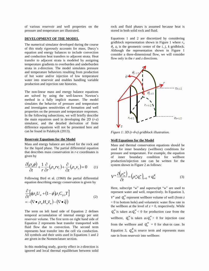
Equations 1 and 2 are discretized by considering

gridblock representation shown in Figure 1 where ri,

j, zk is the geometric center of the i, j, k gridblock.

Although the representation shown in Figure 1

consider a three-dimensional flow, we will consider

flow only in the r and z directions.

Figure 1: 3D (r--z) gridblock illustration.

Well Equations for the Model

Mass and thermal conservation equations should be

used for inner boundary (wellbore) conditions for

pressure and temperature. For example, the equation

of inner boundary condition for wellbore

production/injection rate can be written for the

system shown in Figure 2 as follows:

Rmz

wz

ww

www qqt

V

0

(3)

Here, subscript “w” and superscript “w” are used to

represent water and well, respectively. In Equation 3,

Vw and

wzq represent wellbore volume of well (from z

= 0 to bottom hole) and volumetric water flow rate in

the wellbore at the level of z = 0, respectively. While wzq is taken as

wzq < 0 for production case from the

wellbore, wzq is taken as

wzq > 0 for injection case

from the wellbore and wzq = 0 for shut-in case. In

Equation 3, Rmq is source term and represents mass

rate in from reservoir into wellbore:

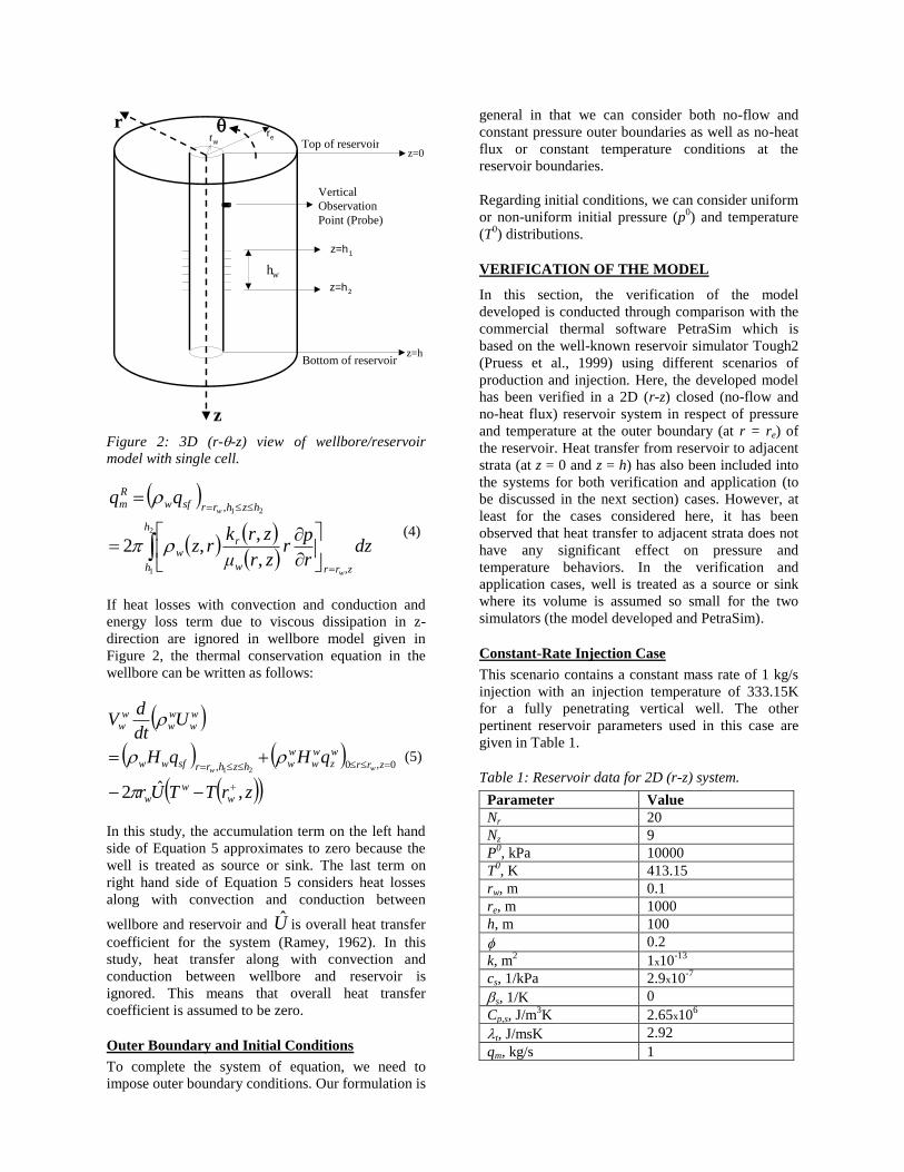
Figure 2: 3D (r--z) view of wellbore/reservoir

model with single cell.

2

1

21

,

,,2

,

h

h ,zrrw

rw

hzhrrsfwRm

dzr

pr

zrμ

zrkrz

qq

w

w

(4)

If heat losses with convection and conduction and

energy loss term due to viscous dissipation in z-

direction are ignored in wellbore model given in

Figure 2, the thermal conservation equation in the

wellbore can be written as follows:

zrTTUr

qHqH

Udt

dV

ww

w

zrr

wz

ww

wwhzhrrsfww

ww

ww

ww

ww

,ˆ2

0,0, 21

(5)

In this study, the accumulation term on the left hand

side of Equation 5 approximates to zero because the

well is treated as source or sink. The last term on

right hand side of Equation 5 considers heat losses

along with convection and conduction between

wellbore and reservoir and U is overall heat transfer

coefficient for the system (Ramey, 1962). In this

study, heat transfer along with convection and

conduction between wellbore and reservoir is

ignored. This means that overall heat transfer

coefficient is assumed to be zero.

Outer Boundary and Initial Conditions

To complete the system of equation, we need to

impose outer boundary conditions. Our formulation is

general in that we can consider both no-flow and

constant pressure outer boundaries as well as no-heat

flux or constant temperature conditions at the

reservoir boundaries.

Regarding initial conditions, we can consider uniform

or non-uniform initial pressure (p0) and temperature

(T0) distributions.

VERIFICATION OF THE MODEL

In this section, the verification of the model

developed is conducted through comparison with the

commercial thermal software PetraSim which is

based on the well-known reservoir simulator Tough2

(Pruess et al., 1999) using different scenarios of

production and injection. Here, the developed model

has been verified in a 2D (r-z) closed (no-flow and

no-heat flux) reservoir system in respect of pressure

and temperature at the outer boundary (at r = re) of

the reservoir. Heat transfer from reservoir to adjacent

strata (at z = 0 and z = h) has also been included into

the systems for both verification and application (to

be discussed in the next section) cases. However, at

least for the cases considered here, it has been

observed that heat transfer to adjacent strata does not

have any significant effect on pressure and

temperature behaviors. In the verification and

application cases, well is treated as a source or sink

where its volume is assumed so small for the two

simulators (the model developed and PetraSim).

Constant-Rate Injection Case

This scenario contains a constant mass rate of 1 kg/s

injection with an injection temperature of 333.15K

for a fully penetrating vertical well. The other

pertinent reservoir parameters used in this case are

given in Table 1.

Table 1: Reservoir data for 2D (r-z) system.

Parameter Value

Nr 20

Nz 9

P0, kPa 10000

T0, K 413.15

rw, m 0.1

re, m 1000

h, m 100

0.2

k, m2 1x10

-13

cs, 1/kPa 2.9x10-7

s, 1/K 0

Cp,s, J/m3K 2.65x10

6

t, J/msK 2.92

qm, kg/s 1

— — — — — —

— — — — — —

z=h 1

z=h 2

z

r r e r w

h w

z=0

z=h

Top of reservoir

Bottom of reservoir

Vertical

Observation

Point (Probe)

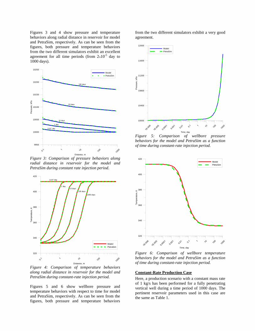
Figures 3 and 4 show pressure and temperature

behaviors along radial distance in reservoir for model

and PetraSim, respectively. As can be seen from the

figures, both pressure and temperature behaviors

from the two different simulators exhibit an excellent

agreement for all time periods (from 2x10-5

day to

1000 days).

Figure 3: Comparison of pressure behaviors along

radial distance in reservoir for the model and

PetraSim during constant rate injection period.

Figure 4: Comparison of temperature behaviors

along radial distance in reservoir for the model and

PetraSim during constant-rate injection period.

Figures 5 and 6 show wellbore pressure and

temperature behaviors with respect to time for model



from the two different simulators exhibit a very good

agreement.

Figure 5: Comparison of wellbore pressure

behaviors for the model and PetraSim as a function

of time during constant-rate injection period.

Figure 6: Comparison of wellbore temperature


of time during constant-rate injection period.

Constant-Rate Production Case

Here, a production scenario with a constant mass rate

of 1 kg/s has been performed for a fully penetrating

vertical well during a time period of 1000 days. The

pertinent reservoir parameters used in this case are

the same as Table 1.

Distance, m

9950

10000

10050

10100

10150

10200

10250

Pre

ssure

,kP

a

Model

PetraSim

2x10-5 day

1 day

10 days

100 days

50 days

Distance, m

320

340

360

380

400

420

Tem

pe

ratu

re,K

Model

PetraSim

100 days

1 day

10 days

2x10-5 day

1000 days

Time, day

10000

10400

10800

11200

11600

12000

Pre

ssure

,kP

a

Model

PetraSim

Time, day

320

340

360

380

400

420

Te

mp

era

ture

,K

Model

PetraSim

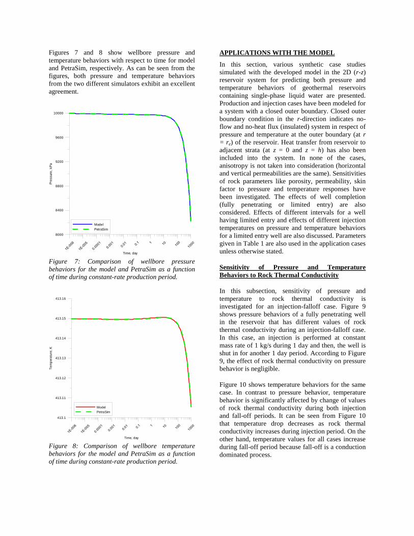
Figures 7 and 8 show wellbore pressure and

temperature behaviors with respect to time for model



from the two different simulators exhibit an excellent

agreement.

Figure 7: Comparison of wellbore pressure


of time during constant-rate production period.

Figure 8: Comparison of wellbore temperature


of time during constant-rate production period.

APPLICATIONS WITH THE MODEL

In this section, various synthetic case studies

simulated with the developed model in the 2D (r-z)

reservoir system for predicting both pressure and

temperature behaviors of geothermal reservoirs

containing single-phase liquid water are presented.

Production and injection cases have been modeled for

a system with a closed outer boundary. Closed outer

boundary condition in the r-direction indicates no-

flow and no-heat flux (insulated) system in respect of

pressure and temperature at the outer boundary (at r

= re) of the reservoir. Heat transfer from reservoir to

adjacent strata (at z = 0 and z = h) has also been

included into the system. In none of the cases,

anisotropy is not taken into consideration (horizontal

and vertical permeabilities are the same). Sensitivities

of rock parameters like porosity, permeability, skin

factor to pressure and temperature responses have

been investigated. The effects of well completion

(fully penetrating or limited entry) are also

considered. Effects of different intervals for a well

having limited entry and effects of different injection

temperatures on pressure and temperature behaviors

for a limited entry well are also discussed. Parameters

given in Table 1 are also used in the application cases

unless otherwise stated.

Sensitivity of Pressure and Temperature

Behaviors to Rock Thermal Conductivity

In this subsection, sensitivity of pressure and

temperature to rock thermal conductivity is

investigated for an injection-falloff case. Figure 9

shows pressure behaviors of a fully penetrating well

in the reservoir that has different values of rock

thermal conductivity during an injection-falloff case.

In this case, an injection is performed at constant

mass rate of 1 kg/s during 1 day and then, the well is

shut in for another 1 day period. According to Figure

9, the effect of rock thermal conductivity on pressure

behavior is negligible.

Figure 10 shows temperature behaviors for the same

case. In contrast to pressure behavior, temperature

behavior is significantly affected by change of values

of rock thermal conductivity during both injection

and fall-off periods. It can be seen from Figure 10

that temperature drop decreases as rock thermal

conductivity increases during injection period. On the

other hand, temperature values for all cases increase

during fall-off period because fall-off is a conduction

dominated process.

Time, day

8000

8400

8800

9200

9600

10000

Pre

ssure

,kP

a

Model

PetraSim

Time, day

413.1

413.11

413.12

413.13

413.14

413.15

413.16

Te

mp

era

ture

,K

Model

PetraSim

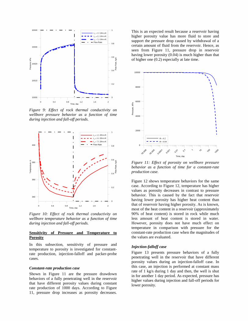
Figure 9: Effect of rock thermal conductivity on

wellbore pressure behavior as a function of time

during injection and fall-off periods.

Figure 10: Effect of rock thermal conductivity on

wellbore temperature behavior as a function of time


Sensitivity of Pressure and Temperature to

Porosity


temperature to porosity is investigated for constant-

rate production, injection-falloff and packer-probe

cases.

Constant-rate production case

Shown in Figure 11 are the pressure drawdown

behaviors of a fully penetrating well in the reservoir

that have different porosity values during constant

rate production of 1000 days. According to Figure

11, pressure drop increases as porosity decreases.

This is an expected result because a reservoir having

higher porosity value has more fluid to store and

support the pressure drop caused by withdrawal of a

certain amount of fluid from the reservoir. Hence, as

seen from Figure 11, pressure drop in reservoir

having lower porosity (0.04) is much higher than that

of higher one (0.2) especially at late time.

Figure 11: Effect of porosity on wellbore pressure

behavior as a function of time for a constant-rate

production case.


case. According to Figure 12, temperature has higher

values as porosity decreases in contrast to pressure

behavior. This is caused by the fact that reservoir

having lower porosity has higher heat content than

that of reservoir having higher porosity. As is known,

most of the heat content in a reservoir (approximately

90% of heat content) is stored in rock while much

less amount of heat content is stored in water.

However, porosity does not have much effect on

temperature in comparison with pressure for the

constant-rate production case when the magnitudes of

the values are evaluated.

Injection-falloff case

Figure 13 presents pressure behaviors of a fully

penetrating well in the reservoir that have different

porosity values during an injection-falloff case. In

this case, an injection is performed at constant mass

rate of 1 kg/s during 1 day and then, the well is shut

in for another 1 day period. As expected, pressure has

higher values during injection and fall-off periods for

lower porosity.

0 0.4 0.8 1.2 1.6 2Time, day

10000

10010

10020

10030

10040P

ressu

re,

kP

a

s J/m-s-K

s J/m-s-K

s J/m-s-K

Flow Rate

0

0.2

0.4

0.6

0.8

1

Flo

wR

ate

,kg

/s

0 0.4 0.8 1.2 1.6 2Time, day

340

360

380

400

Tem

pe

ratu

re,

K

s J/m-s-K

s J/m-s-K

s J/m-s-K

Flow Rate

0

0.2

0.4

0.6

0.8

1

Flo

wR

ate

,kg

/s

Time, day

0

2000

4000

6000

8000

10000

Pre

ssure

,kP

a

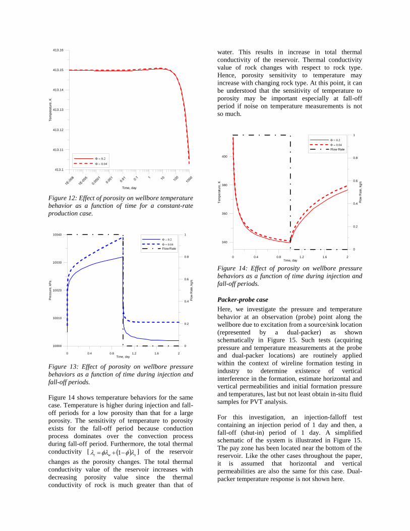
Figure 12: Effect of porosity on wellbore temperature

behavior as a function of time for a constant-rate

production case.


behaviors as a function of time during injection and

fall-off periods.


case. Temperature is higher during injection and fall-

off periods for a low porosity than that for a large

porosity. The sensitivity of temperature to porosity

exists for the fall-off period because conduction

process dominates over the convection process

during fall-off period. Furthermore, the total thermal

conductivity [ swt 1 ] of the reservoir

changes as the porosity changes. The total thermal

conductivity value of the reservoir increases with

decreasing porosity value since the thermal

conductivity of rock is much greater than that of

water. This results in increase in total thermal

conductivity of the reservoir. Thermal conductivity

value of rock changes with respect to rock type.

Hence, porosity sensitivity to temperature may

increase with changing rock type. At this point, it can

be understood that the sensitivity of temperature to

porosity may be important especially at fall-off

period if noise on temperature measurements is not

so much.


behaviors as a function of time during injection and

fall-off periods.

Packer-probe case

Here, we investigate the pressure and temperature

behavior at an observation (probe) point along the

wellbore due to excitation from a source/sink location

(represented by a dual-packer) as shown

schematically in Figure 15. Such tests (acquiring

pressure and temperature measurements at the probe

and dual-packer locations) are routinely applied

within the context of wireline formation testing in

industry to determine existence of vertical

interference in the formation, estimate horizontal and

vertical permeabilities and initial formation pressure

and temperatures, last but not least obtain in-situ fluid

samples for PVT analysis.

For this investigation, an injection-falloff test

containing an injection period of 1 day and then, a

fall-off (shut-in) period of 1 day. A simplified

schematic of the system is illustrated in Figure 15.

The pay zone has been located near the bottom of the

reservoir. Like the other cases throughout the paper, it is assumed that horizontal and vertical

permeabilities are also the same for this case. Dual-

packer temperature response is not shown here.

Time, day

413.1

413.11

413.12

413.13

413.14

413.15

413.16T

em

pera

ture

,K

0 0.4 0.8 1.2 1.6 2Time, day

10000

10010

10020

10030

10040

Pre

ssu

re,

kP

a

Flow Rate

0

0.2

0.4

0.6

0.8

1

Flo

wR

ate

,kg

/s

0 0.4 0.8 1.2 1.6 2Time, day

340

360

380

400

Tem

pe

ratu

re,

K

Flow Rate

0

0.2

0.4

0.6

0.8

1

Flo

wR

ate

,kg

/s

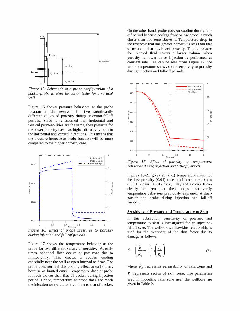
Figure 15: Schematic of a probe configuration of a

packer-probe wireline formation tester for a vertical

well.

Figure 16 shows pressure behaviors at the probe

location in the reservoir for two significantly

different values of porosity during injection-falloff

periods. Since it is assumed that horizontal and

vertical permeabilities are the same, then pressure for

the lower porosity case has higher diffusivity both in

the horizontal and vertical directions. This means that

the pressure increase at probe location will be more

compared to the higher porosity case.

Figure 16: Effect of probe pressures to porosity


Figure 17 shows the temperature behavior at the

probe for two different values of porosity. At early

times, spherical flow occurs at pay zone due to

limited-entry. This creates a sudden cooling

especially near the well at open interval to flow. The

probe does not feel this cooling effect at early times

because of limited-entry. Temperature drop at probe

is much slower than that of packer during injection

period. Hence, temperature at probe does not reach

the injection temperature in contrast to that of packer.

On the other hand, probe goes on cooling during fall-

off period because cooling front below probe is much

closer than hot zone above it. Temperature drop in

the reservoir that has greater porosity is less than that

of reservoir that has lower porosity. This is because

the injected fluid covers a larger volume when

porosity is lower since injection is performed at

constant rate. As can be seen from Figure 17, the

probe temperature shows some sensitivity to porosity


Figure 17: Effect of porosity on temperature

behaviors during injection and fall-off periods.

Figures 18-21 gives 2D (r-z) temperature maps for

the low porosity (0.04) case at different time steps

(0.03162 days, 0.5012 days, 1 day and 2 days). It can

clearly be seen that these maps also verify

temperature behaviors previously explained at dual-

packer and probe during injection and fall-off

periods.

Sensitivity of Pressure and Temperature to Skin


temperature to skin is investigated for an injection-

falloff case. The well-known Hawkins relationship is

used for the treatment of the skin factor due to

damage as follows:

w

s

s r

r

k

kS ln1 (6)

where sk represents permeability of skin zone and

sr represents radius of skin zone. The parameters

used in modeling skin zone near the wellbore are

given in Table 2.

Packer hw =3 m

z0 =6 m

h =100 m

Probe

zw=0.4 m

0 0.4 0.8 1.2 1.6 2Time, day

10000

10020

10040

10060

Pre

ssu

re,

kP

a

Probe ( )

Probe ( )

Flow Rate, kg/s

0

0.2

0.4

0.6

0.8

1

Flo

wR

ate

,kg

/s

0 0.4 0.8 1.2 1.6 2Time, day

407

408

409

410

411

412

413

414

Tem

pe

ratu

re,

K

Probe ( = 0.2)

Probe ( = 0.04)

Flow Rate

0

0.2

0.4

0.6

0.8

1

Flo

wR

ate

,kg

/s

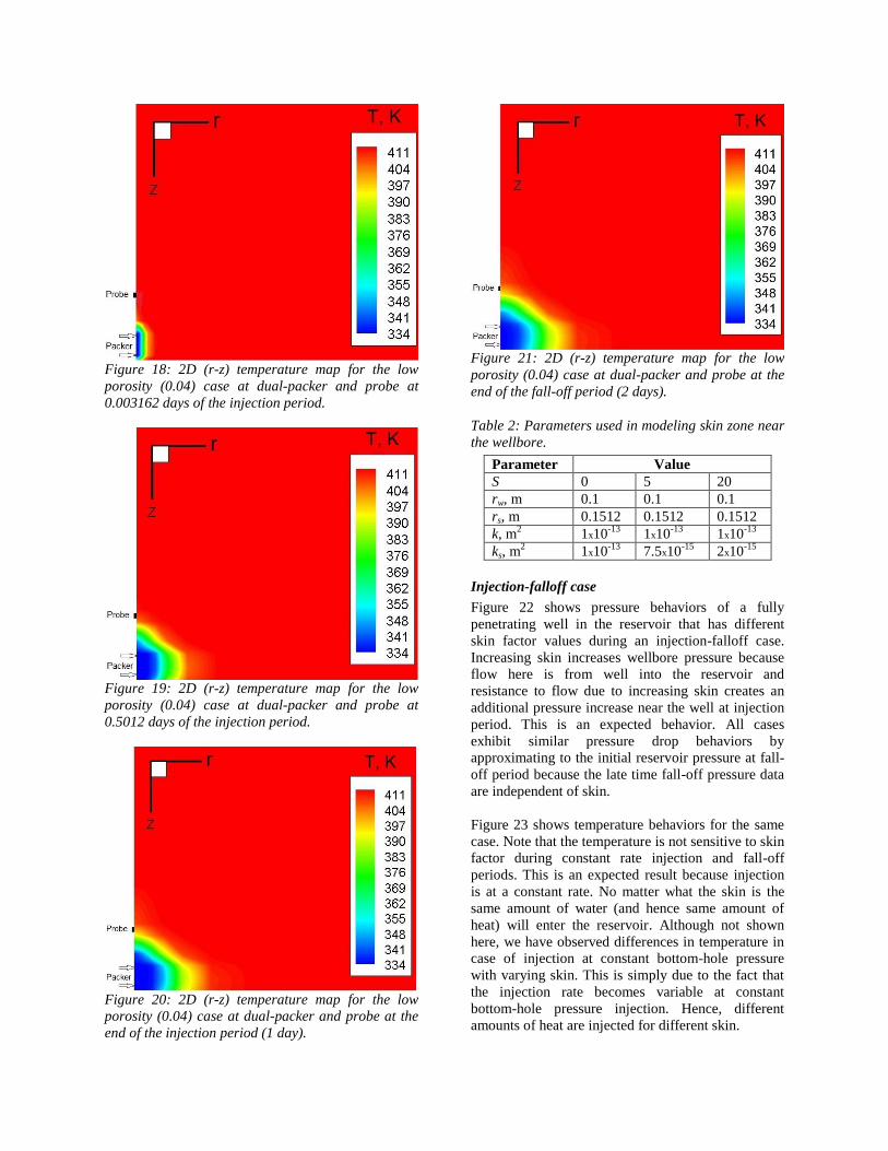
Figure 18: 2D (r-z) temperature map for the low

porosity (0.04) case at dual-packer and probe at

0.003162 days of the injection period.


porosity (0.04) case at dual-packer and probe at

0.5012 days of the injection period.


porosity (0.04) case at dual-packer and probe at the

end of the injection period (1 day).


porosity (0.04) case at dual-packer and probe at the

end of the fall-off period (2 days).

Table 2: Parameters used in modeling skin zone near

the wellbore.

Parameter Value

S 0 5 20

rw, m 0.1 0.1 0.1

rs, m 0.1512 0.1512 0.1512

k, m2 1x10

-13 1x10

-13 1x10

-13

ks, m2 1x10

-13 7.5x10

-15 2x10

-15


Figure 22 shows pressure behaviors of a fully

penetrating well in the reservoir that has different

skin factor values during an injection-falloff case.

Increasing skin increases wellbore pressure because

flow here is from well into the reservoir and

resistance to flow due to increasing skin creates an

additional pressure increase near the well at injection

period. This is an expected behavior. All cases

exhibit similar pressure drop behaviors by

approximating to the initial reservoir pressure at fall-

off period because the late time fall-off pressure data

are independent of skin.


case. Note that the temperature is not sensitive to skin

factor during constant rate injection and fall-off

periods. This is an expected result because injection

is at a constant rate. No matter what the skin is the

same amount of water (and hence same amount of

heat) will enter the reservoir. Although not shown

here, we have observed differences in temperature in

case of injection at constant bottom-hole pressure

with varying skin. This is simply due to the fact that

the injection rate becomes variable at constant

bottom-hole pressure injection. Hence, different

amounts of heat are injected for different skin.

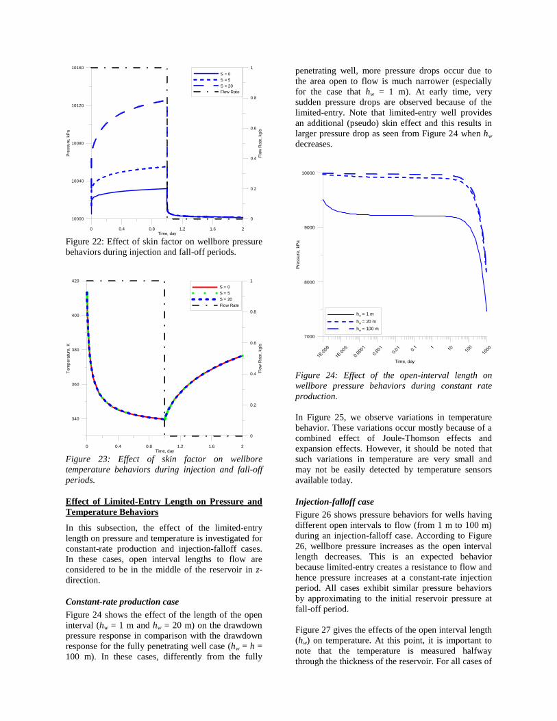
Figure 22: Effect of skin factor on wellbore pressure

behaviors during injection and fall-off periods.

Figure 23: Effect of skin factor on wellbore

temperature behaviors during injection and fall-off

periods.

Effect of Limited-Entry Length on Pressure and

Temperature Behaviors

In this subsection, the effect of the limited-entry

length on pressure and temperature is investigated for

constant-rate production and injection-falloff cases.

In these cases, open interval lengths to flow are

considered to be in the middle of the reservoir in z-

direction.

Constant-rate production case

Figure 24 shows the effect of the length of the open

interval (hw = 1 m and hw = 20 m) on the drawdown

pressure response in comparison with the drawdown

response for the fully penetrating well case (hw = h =

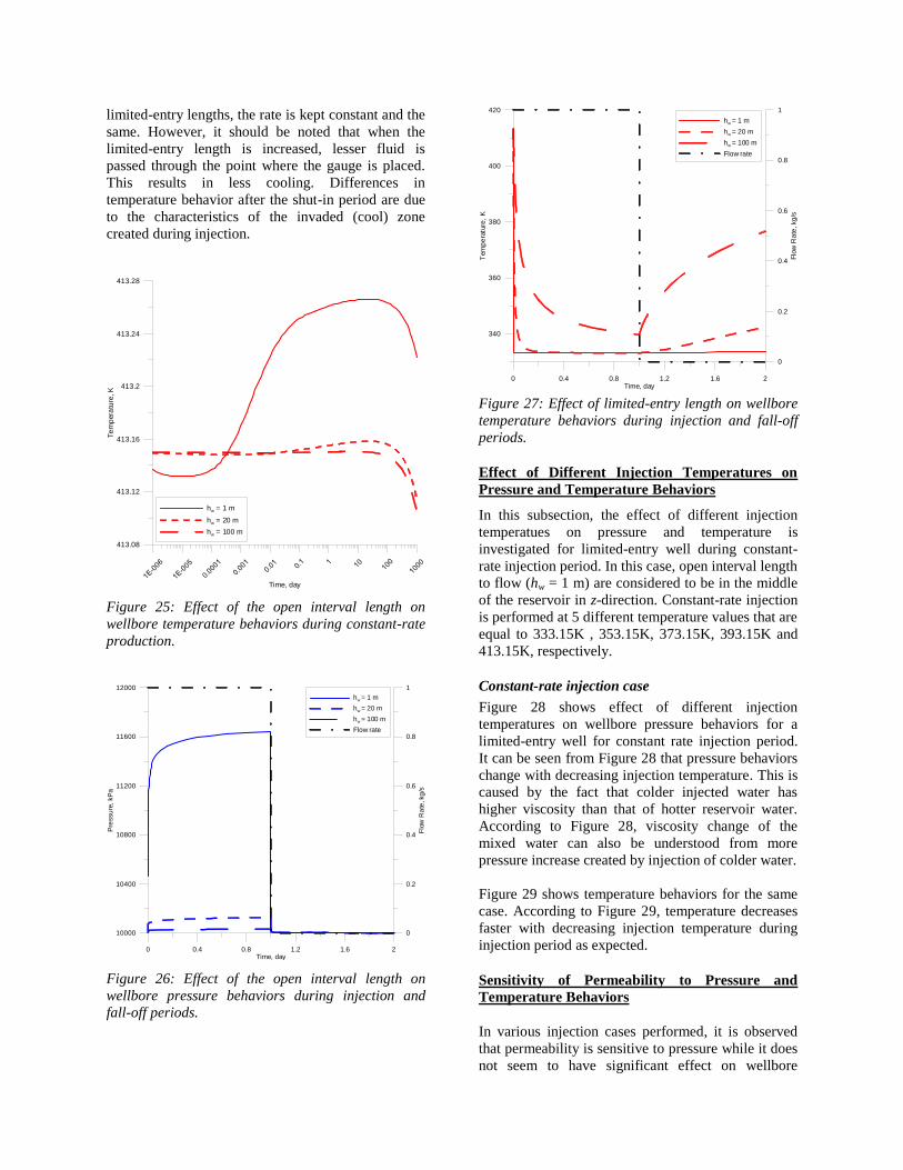
100 m). In these cases, differently from the fully

penetrating well, more pressure drops occur due to

the area open to flow is much narrower (especially

for the case that hw = 1 m). At early time, very

sudden pressure drops are observed because of the

limited-entry. Note that limited-entry well provides

an additional (pseudo) skin effect and this results in

larger pressure drop as seen from Figure 24 when hw

decreases.

Figure 24: Effect of the open-interval length on

wellbore pressure behaviors during constant rate

production.

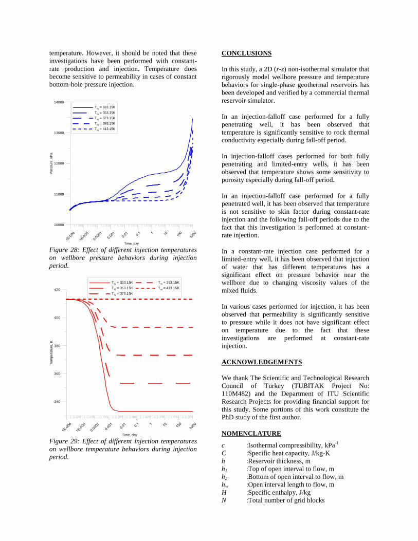
In Figure 25, we observe variations in temperature

behavior. These variations occur mostly because of a

combined effect of Joule-Thomson effects and

expansion effects. However, it should be noted that

such variations in temperature are very small and

may not be easily detected by temperature sensors

available today.


Figure 26 shows pressure behaviors for wells having

different open intervals to flow (from 1 m to 100 m)

during an injection-falloff case. According to Figure

26, wellbore pressure increases as the open interval

length decreases. This is an expected behavior

because limited-entry creates a resistance to flow and

hence pressure increases at a constant-rate injection

period. All cases exhibit similar pressure behaviors

by approximating to the initial reservoir pressure at

fall-off period.

Figure 27 gives the effects of the open interval length

(hw) on temperature. At this point, it is important to

note that the temperature is measured halfway

through the thickness of the reservoir. For all cases of

0 0.4 0.8 1.2 1.6 2Time, day

10000

10040

10080

10120

10160P

ressu

re,

kP

a

S = 0

S = 5

S = 20

Flow Rate

0

0.2

0.4

0.6

0.8

1

Flo

wR

ate

,kg

/s

0 0.4 0.8 1.2 1.6 2Time, day

340

360

380

400

420

Tem

pe

ratu

re,

K

S = 0

S = 5

S = 20

Flow Rate

0

0.2

0.4

0.6

0.8

1

Flo

wR

ate

,kg

/s

Time, day

7000

8000

9000

10000

Pre

ssure

,kP

a

hw = 1 m

hw = 20 m

hw = 100 m

limited-entry lengths, the rate is kept constant and the

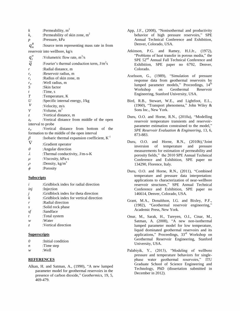
same. However, it should be noted that when the

limited-entry length is increased, lesser fluid is

passed through the point where the gauge is placed.

This results in less cooling. Differences in

temperature behavior after the shut-in period are due

to the characteristics of the invaded (cool) zone

created during injection.

Figure 25: Effect of the open interval length on

wellbore temperature behaviors during constant-rate

production.

Figure 26: Effect of the open interval length on

wellbore pressure behaviors during injection and

fall-off periods.

Figure 27: Effect of limited-entry length on wellbore

temperature behaviors during injection and fall-off

periods.

Effect of Different Injection Temperatures on

Pressure and Temperature Behaviors

In this subsection, the effect of different injection

temperatues on pressure and temperature is

investigated for limited-entry well during constant-

rate injection period. In this case, open interval length

to flow (hw = 1 m) are considered to be in the middle

of the reservoir in z-direction. Constant-rate injection

is performed at 5 different temperature values that are

equal to 333.15K , 353.15K, 373.15K, 393.15K and

413.15K, respectively.

Constant-rate injection case

Figure 28 shows effect of different injection

temperatures on wellbore pressure behaviors for a

limited-entry well for constant rate injection period.

It can be seen from Figure 28 that pressure behaviors

change with decreasing injection temperature. This is

caused by the fact that colder injected water has

higher viscosity than that of hotter reservoir water.

According to Figure 28, viscosity change of the

mixed water can also be understood from more

pressure increase created by injection of colder water.


case. According to Figure 29, temperature decreases

faster with decreasing injection temperature during

injection period as expected.

Sensitivity of Permeability to Pressure and

Temperature Behaviors

In various injection cases performed, it is observed

that permeability is sensitive to pressure while it does

not seem to have significant effect on wellbore

Time, day

413.08

413.12

413.16

413.2

413.24

413.28

Te

mp

era

ture

,K

hw = 1 m

hw = 20 m

hw = 100 m

0 0.4 0.8 1.2 1.6 2Time, day

10000

10400

10800

11200

11600

12000

Pre

ssu

re,

kP

a

hw = 1 m

hw = 20 m

hw = 100 m

Flow rate

0

0.2

0.4

0.6

0.8

1

Flo

wR

ate

,kg

/s

0 0.4 0.8 1.2 1.6 2Time, day

340

360

380

400

420

Tem

pe

ratu

re,

K

hw = 1 m

hw = 20 m

hw = 100 m

Flow rate

0

0.2

0.4

0.6

0.8

1

Flo

wR

ate

,kg

/s

temperature. However, it should be noted that these

investigations have been performed with constant-

rate production and injection. Temperature does

become sensitive to permeability in cases of constant

bottom-hole pressure injection.

Figure 28: Effect of different injection temperatures

on wellbore pressure behaviors during injection

period.

Figure 29: Effect of different injection temperatures

on wellbore temperature behaviors during injection

period.

CONCLUSIONS

In this study, a 2D (r-z) non-isothermal simulator that

rigorously model wellbore pressure and temperature

behaviors for single-phase geothermal reservoirs has

been developed and verified by a commercial thermal

reservoir simulator.

In an injection-falloff case performed for a fully

penetrating well, it has been observed that

temperature is significantly sensitive to rock thermal

conductivity especially during fall-off period.

In injection-falloff cases performed for both fully

penetrating and limited-entry wells, it has been

observed that temperature shows some sensitivity to

porosity especially during fall-off period.

In an injection-falloff case performed for a fully

penetrated well, it has been observed that temperature

is not sensitive to skin factor during constant-rate

injection and the following fall-off periods due to the

fact that this investigation is performed at constant-

rate injection.

In a constant-rate injection case performed for a

limited-entry well, it has been observed that injection

of water that has different temperatures has a

significant effect on pressure behavior near the

wellbore due to changing viscosity values of the

mixed fluids.

In various cases performed for injection, it has been

observed that permeability is significantly sensitive

to pressure while it does not have significant effect

on temperature due to the fact that these

investigations are performed at constant-rate

injection.

ACKNOWLEDGEMENTS

We thank The Scientific and Technological Research

Council of Turkey (TUBITAK Project No:

110M482) and the Department of ITU Scientific

Research Projects for providing financial support for

this study. Some portions of this work constitute the

PhD study of the first author.

NOMENCLATURE

c :Isothermal compressibility, kPa-1

C :Specific heat capacity, J/kg-K

h :Reservoir thickness, m

h1 :Top of open interval to flow, m

h2 :Bottom of open interval to flow, m

hw :Open interval length to flow, m

H :Specific enthalpy, J/kg

N :Total number of grid blocks

Time, day

10000

11000

12000

13000

14000

Pre

ssure

,kP

a

Tinj

= 333.15K

T inj = 353.15K

T inj = 373.15K

T inj = 393.15K

T inj = 413.15K

Time, day

340

360

380

400

420

Te

mpe

ratu

re,

K

T inj = 333.15K

T inj = 353.15K

T inj = 373.15K

Tinj = 393.15K

Tinj = 413.15K

k :Permeability, m2

ks :Permeability of skin zone, m2

p :Pressure, kPa Rmq :Source term representing mass rate in from

reservoir into wellbore, kg/s wzq :Volumetric flow rate, m

3/s

q~ :Fourier’s thermal conduction term, J/m2s

r :Radial distance, m

re :Reservoir radius, m

rs :Radius of skin zone, m

rw :Well radius, m

S :Skin factor

t :Time, s

T :Temperature, K

U :Specific internal energy, J/kg v :Velocity, m/s

V :Volume, m3

z :Vertical distance, m

z0 :Vertical distance from middle of the open

interval to probe

zw :Vertical distance from bottom of the

formation to the middle of the open interval

:Isobaric thermal expansion coefficient, K-1

:Gradient operator

:Angular direction

:Thermal conductivity, J/m-s-K

:Viscosity, kPa-s

:Density, kg/m3

:Porosity

Subscripts

i :Gridblock index for radial direction

inj :Injection

j :Gridblock index for theta direction

k :Gridblock index for vertical direction

r :Radial direction

s :Solid rock phase

sf :Sandface

t :Total system

w :Water

z :Vertical direction

Superscripts

0 :Initial condition

n :Time step

w :Well

REFERENCES

Alkan, H. and Satman, A., (1990), “A new lumped

parameter model for geothermal reservoirs in the

presence of carbon dioxide,” Geothermics, 19, 5,

469-479.

App, J.F., (2008), “Nonisothermal and productivity

behavior of high pressure reservoirs,” SPE

Annual Technical Conference and Exhibition,

Denver, Colorado, USA.

Atkinson, P.G. and Ramey, H.J.Jr., (1972),

“Problems of heat transfer in porous media,” the

SPE 52nd

Annual Fall Technical Conference and

Exhibition, SPE paper no 6792, Denver,

Colorado.

Axelsson, G., (1989), “Simulation of pressure

response data from geothermal reservoirs by

lumped parameter models,” Proceedings, 14th

Workshop on Geothermal Reservoir

Engineering, Stanford University, USA.

Bird, R.B., Stewart, W.E., and Lightfoot, E.L.,

(1960), “Transport phenomena,” John Wiley &

Sons Inc., New York.

Duru, O.O. and Horne, R.N., (2010a), “Modelling

reservoir temperature transients and reservoir-

parameter estimation constrained to the model,”

SPE Reservoir Evaluation & Engineering, 13, 6,

873-883.

Duru, O.O. and Horne, R.N., (2010b),“Joint

inversion of temperature and pressure

measurements for estimation of permeability and

porosity fields,” the 2010 SPE Annual Technical

Conference and Exhibition, SPE paper no

134290, Florence, Italy.

Duru, O.O. and Horne, R.N., (2011), “Combined

temperature and pressure data interpretation:

applications to characterization of near-wellbore

reservoir structures,” SPE Annual Technical


146614, Denver, Colorado, USA.

Grant, M.A., Donaldson, I.G. and Bixley, P.F.,

(1982), “Geothermal reservoir engineering,”

Academic Press, New York.

Onur, M., Sarak, H., Tureyen, O.I., Cinar, M.,

Satman, A. (2008), “A new non-isothermal

lumped parameter model for low temperature,

liquid dominated geothermal reservoirs and its

applications,” Proceedings, 33rd

Workshop on

Geothermal Reservoir Engineering, Stanford

University, USA.

Palabiyik, Y., (2013), “Modeling of wellbore

pressure and temperature behaviors for single-

phase water geothermal reservoirs,” ITU

Graduate School of Science Engineering and

Technology, PhD (dissertation submitted in

December in 2012).

Petrasim, (2011), “User manual, Version 5,”

Thunderhead Engineering Consultants,

Rockware Inc., Manhattan, USA.

Pruess, K., Oldenburg, C. and Moridis, G., (1999),

“Tough2 user’s guide version 2.0,” Report 476,

LBNL-43134,” Lawrence Berkeley National

Laboratory, Berkeley, California, USA.

Ramazanov, A.Sh., Valiullin, R.A., Sadretdinov

A.A., Shako, V.V., Pimenov, V.P., Fedorov,

V.N. and Belov, K.V., (2010), “Thermal

modeling for characterization of near wellbore

zone and zonal allocation,” the 2010 SPE

Russian Oil & Gas Technical Conference and

Exhibition, SPE paper no 136256, Moscow,

Russia.

Ramey, H.J.Jr. (1962), “Wellbore Heat

Transmission,” Journal of Petroleum

Technology, 14, 4, 427-435.

Sarak, H., Onur, M. and Satman, A., (2005),

“Lumped-parameter models for low temperature

geothermal reservoirs and their application,”

Geothermics, 34, 728-755.

Sui, W., Zhu, D., Hill, A.D. and Ehlig-Economides,

C, (2008a), “Model for transient temperature and

pressure behavior in commingled vertical wells,”

SPE Russian Oil & Gas Technical Conference

and Exhibition, SPE paper no 115200, Moscow,

Russia.

Sui, W., Zhu, D., Hill, A.D. and Ehlig-Economides,

C, (2008b), “Determining multilayer formation

properties from transient temperature and

pressure measurements,” SPE Annual Technical


116270, Denver, Colorado, USA.

Tureyen, O.I., Onur, M. and Sarak, H., (2009), “A

Generalized non-isothermal lumped parameter

model for liquid dominated geothermal

reservoirs,” Proceedings, 34th Workshop on

Geothermal Reservoir Engineering, Stanford

University, USA.

Tureyen, O.I., Sarak, H. and Onur, M., (2007),

“Assessing uncertainty in future pressure

changes predicted by lumped-parameter models:

a field application,” Proceedings, 32nd

Workshop on Geothermal Reservoir

Engineering, Stanford University, USA.

Documents

A Study on Pressure and Temperature Behaviors of ... · A STUDY ON PRESSURE AND TEMPERATURE BEHAVIORS OF ... of reservoir fluids ... to study temperature behavior for the case of