A STUDY OF UNUSUAL METABOLIC VARIANTS OF AEROMONAS

ABSTRACT

Title of Document: A STUDY OF UNUSUAL METABOLIC

VARIANTS OF AEROMONAS CAVIAE AND

AEROMONAS HYDROPHILA USING A

POLYPHASIC TAXONOMIC APPROACH Zenas Chang, MS, 2010 Directed By: Professor Sam W. Joseph, CBMG

Variation in acid production from carbohydrate metabolism has been identified in

Aeromonas as a potential indicator for new subspecies. Therefore, pure cultures of

non-lactose fermenting Aeromonas caviae, a cause of waterborne infections in

humans and other vertebrates, were studied after noting a mixture of acid producing

and non-acid producing colonies after four days of incubation on MacConkey agar at

ambient temperature. Unusual arabinose negative strains of A. hydrophila (usually

arabinose positive) were added to the project to further study the correlation between

carbohydrate fermentation and taxonomy. These metabolic variants of A. caviae and

A. hydrophila were studied for phenotypic differences via carbohydrate utilization

assays as well as genotypic differences via FAFLP. The results suggest that the A.

caviae isolates MB3 and MB7 should be considered novel subspecies, while the

arabinose negative strain designated A. hydrophila subsp. dhakensis is correctly

identified as a subspecies of A. hydrophila.

A STUDY OF UNUSUAL METABOLIC VARIANTS OF AEROMONAS CAVIAE

AND AEROMONAS HYDROPHILA USING A POLYPHASIC TAXONOMIC APPROACH

By

Zenas Chang

Thesis submitted to the Faculty of the Graduate School of the University of Maryland, College Park, in partial fulfillment

of the requirements for the degree of Master of Science

2010 Advisory Committee: Professor Sam W. Joseph, Chair Professor Anwar Huq Professor Daniel C. Stein

© Copyright by Zenas Chang

2010

ii

DEDICATION

I dedicate this thesis to my parents, Chao-hsi and Hui-yen, and my sister, Zanetta. I would not have made it this far without all of their support and encouragement. I would also like to dedicate this project to Dr. Sam W. Joseph, who taught me all about the world of scientific research; without his infinite knowledge and patience I would not have been able to finish this degree.

iii

ACKNOWLEDGEMENTS

I would like to thank:

Dr. Sam W. Joseph, my advisor and a close friend. I am greatly inspired by

his knowledge of the field of microbiology and I hope to emulate his success one day.

Dr. Anwar Huq and Dr. Daniel C. Stein for their willingness to serve on my

thesis committee and for their advice and support. I would also like to acknowledge

Ms. Sarah Biancardi for all of her administrative aid.

Dr. Amy Horneman for sharing her wealth of knowledge about Aeromonas,

Dr. Christopher Grimm for all of his patience and instruction in the field of molecular

biology, and Dr. Julie Hebert from Dr. David Hawthorne’s lab for her aid with the

FAFLP technique.

Dr. Amy Sapkota and Dr. Shirley Micallef for their advice and guidance.

Norman Wang and Zanetta Chang for their technical assistance.

iv

TABLE OF CONTENTS

DEDICATION ............................................................................................................................. II

ACKNOWLEDGEMENTS ............................................................................................................ III

TABLE OF CONTENTS ............................................................................................................... IV

LIST OF TABLES ....................................................................................................................... VI

LIST OF FIGURES ..................................................................................................................... VII

INTRODUCTION ......................................................................................................................... 1

Aeromonas Physiology and Biochemical Profile ............................................................................. 1

Aeromonas Virulence and Pathology ................................................................................................... 1

Taxonomy Overview .................................................................................................................................. 3

Importance of Proper Taxonomic Designation in Epidemiology and Research................ 4

Historical Taxonomy .................................................................................................................................. 4

Taxonomy Reform ....................................................................................................................................... 6

Taxonomy Refinement .............................................................................................................................. 8

Molecular Identification Methods ..................................................................................................... 14

Aeromonas hydrophila ............................................................................................................................ 15

Aeromonas caviae ..................................................................................................................................... 15

Scope of Project ......................................................................................................................................... 16

Aeromonas caviae ................................................................................................................................ 16

Aeromonas hydrophila subsp. dhakensis .................................................................................... 17

Hypothesis ................................................................................................................................................... 19

MATERIALS AND METHODS .................................................................................................. 20

Aeromonas Strains .................................................................................................................................... 20

Media and Growth Conditions ............................................................................................................ 20

Strain Identification ................................................................................................................................. 21

Strains for A. hydrophila analysis.................................................................................................. 21

A. caviae metabolic variants ............................................................................................................ 22

Invasion Assay (A. caviae) ..................................................................................................................... 22

Agarose Gel Electrophoresis (A. hydrophila and A. caviae) ..................................................... 24

Polyphasic Phenotyping ........................................................................................................................ 25

ONPG (A. caviae) .................................................................................................................................. 25

Carbohydrate Utilization (A. hydrophila and A. caviae)....................................................... 25

Fluorescent Amplified Fragment Length Polymorphism (FAFLP) analysis of A.

hydrophila and A. caviae) ................................................................................................................. 26

RESULTS ................................................................................................................................. 34

A. caviae Variant Activity on Lactose ................................................................................................ 34

A. caviae Tissue Cell Invasion .............................................................................................................. 35

DNA Sample Purification ....................................................................................................................... 36


ONPG Utilization by A. caviae strains .......................................................................................... 36

Sugar Utilization by Aeromonas strains ..................................................................................... 37

FAFLP ....................................................................................................................................................... 37

DISCUSSION ............................................................................................................................ 50

A. caviae Variant Identification ........................................................................................................... 50

Tissue Cell Invasion ................................................................................................................................. 52

v


ONPG and Lactose Utilization by A. caviae Strains ................................................................ 55

Sugar Utilization by A. hydrophila strains ................................................................................. 58

FAFLP ....................................................................................................................................................... 61

Conclusions ............................................................................................................................................ 65

APPENDIX A ........................................................................................................................... 66

APPENDIX B ........................................................................................................................... 68

APPENDIX C ........................................................................................................................... 69

APPENDIX D .......................................................................................................................... 70

APPENDIX E ........................................................................................................................... 72

APPENDIX F ........................................................................................................................... 73

BIBLIOGRAPHY ...................................................................................................................... 81

vi

LIST OF TABLES

TABLE I – LIST OF AEROMONAS STRAINS FOR AFLP ..................................................................... 32

TABLE II – LIST OF A. CAVIAE METABOLIC VARIANTS ................................................................... 33

TABLE III – A. CAVIAE ACTIVITY ON MACCONKEY AGAR .............................................................. 39

TABLE IV – A. CAVIAE TISSUE CELL INVASION AND CELL ASSOCIATIONA .................................... 40

TABLE V – ONPG HYDROLYSIS ........................................................................................................ 41

TABLE VI – L-ARABINOSE UTILIZATION ......................................................................................... 42

TABLE VII –LACTOSE UTILIZATION ................................................................................................. 43

TABLE VIII – L-FUCOSE UTILIZATION ............................................................................................. 44

TABLE IX - GENEMAPPER IDENTIFIED ALLELES ............................................................................ 45

vii

LIST OF FIGURES

FIGURE I – CONFIRMATION OF DNA STOCK CONCENTRATIONS .................................................. 46

FIGURE II – CONFIRMATION OF DIGESTION PROCEDURE .............................................................. 47

FIGURE III – SAMPLE A DENDROGRAM ........................................................................................... 48

FIGURE IV – SAMPLE B DENDROGRAM ........................................................................................... 49

1

INTRODUCTION

Aeromonas Physiology and Biochemical Profile

As described in the most recent edition of Bergey’s Manual of Systematic

Bacteriology, aeromonads are gram-negative, oxidase-positive, glucose-fermenting,

facultatively anaerobic rods belonging to the family Aeromonadaceae (Martin-

Carnahan and Joseph, 2005). As most Aeromonas species are mesophilic and

motile, these organisms are ubiquitous in fresh, brackish, chlorinated, and non-

chlorinated water and have been isolated from estuarine and marine water sources

around the world. Aeromonads are more numerous during the warmer parts of the

year and can be found in a variety of sources ranging from biofilms, biosolids, and

sewage, to raw meat, fish, seafood, and vegetables (Hazen et al. 1978; Seidler et al.

1980; van der Kooj, 1988; Kaper et al. 1981; Holmes and Niccolls, 1995; Holmes et

al., 1996).

Aeromonas Virulence and Pathology

Aeromonas species possess a diverse array of virulence factors: various

endotoxins, hemolysins, enterotoxins, and adherence factors have been identified,

though the precise role of each factor in pathogenesis is currently unknown.

Aeromonads use these virulence factors to cause either primary or opportunistic

disease in a variety of vertebrate and invertebrate hosts. Due to the abundance of

2

Aeromonas in aquatic environments, it is not surprising that Aeromonas spp. has

been isolated from aquatic organisms including frogs, freshwater and saltwater fish,

and even leeches (Sanarelli, 1891; Caselitz, 1955; Gosling, 1996a; Austin and Adams,

1996; Graf, 1999a; Huys et al. 2003, Martinez-Murcia et al. 2008). In fish and frogs,

this microbe has been shown to cause the formation of lesions and cellulitis (Joseph

and Carnahan, 1994; Huys et al. 2003; Martinez-Murcia et al. 2008).

The human pathology associated with Aeromonas falls largely into two

groups: gastroenteritis and wound infections, both of which can occur with or

without bacteremia. In healthy humans, especially children, gastroenteritis is the

most common manifestation, usually following the ingestion of contaminated water

or food. However, Aeromonas also has the capability to cause wound infections

(following exposure to contaminated water) and more serious systemic disease

(peritonitis, sepsis, or meningitis). Sepsis, peritonitis, and meningitis generally arise

secondary to other conditions but are associated with high mortality rates; mortality

is especially high in patients with liver cirrhosis, underlying disease, or in patients

who are immunocompromised (Janda and Abbott, 1996; Janda and Abbott, 1998;

Janda and Abbott, 2010; Altwegg 1999). Aeromonas spp. were also isolated from

wounds of tsunami victims in Thailand (Hiransuthikul et al. 2005) and species

capable of causing necrotizing fasciitis were found in floodwater samples during

Hurricane Katrina in New Orleans (Presley et al. 2006).

3

Taxonomy Overview

Historically, Aeromonas taxonomy was very convoluted, but over the past

twenty years it has been much more clearly elucidated. Currently, there are

approximately eighteen species as defined at the phenospecies level, compared to

approximately seventeen hybridization groups (HGs), or genomospecies, when

classified by DNA homology (Martinez-Murcia et al. 2008). Most phenospecies of

Aeromonas are associated to some extent with human disease; however, the most

important human pathogens are A. hydrophila, A. caviae, and A. veronii biovar

sobria.

The various aeromonads fall into two major groups: motile, mesophilic

organisms first described broadly as A. hydrophila, and non-motile, psychrophilic

aeromonads originally classified as A. salmonicida. While non-motile aeromonads

present with characteristics infrequently observed in other Aeromonas species, DNA

hybridization studies indicated that these organisms are still closely related to the

motile aeromonads (MacInnes et al., 1979). This observation suggests that

organisms belonging to the genus Aeromonas are derived from two major

evolutionary branches: a relatively homogenous group of non-motile organisms

belonging to A. salmonicida, and a diverse group of motile aeromonads

encompassed by the remaining Aeromonas species.

4

Importance of Proper Taxonomic Designation in Epidemiology and

Research

The importance of identifying organisms to the species and sub-species level

when tracking organisms in disease outbreaks cannot be understated. In the clinical

setting, accurate identification of an isolate through the use of proper taxonomic

designation allows for better diagnosis and increased efficacy during treatment.

Likewise, in research, it is highly important to identify the exact organism of interest

before investing a large amount of time and resources into a project. Therefore,

developing precise taxonomical systems and identifying new species and subspecies

serve not only to satisfy scientific curiosity, but also to improve medical treatment

and the efficiency of future research. This aspect of taxonomy has become so

important that an increasing variety of molecular, serologic, phage typing and other

methods have been implemented in order to classify various species of bacteria.

Recent cases in point include Salmonella isolation in foodborne outbreaks along with

recognition of Yersinia enterocolitica, Aeromonas, and Staphylococcccus aureus

subtypes (Peterson et al. 2010; Neubauer et al. 2001; Huys et al. 2002; Martinez-

Murcia et al. 2008; Hirose et al. 2010).

Historical Taxonomy

The first description of a motile aeromonad was reported by Sanarelli in

1891, when he isolated a bacterium from an infected frog which he termed Bacillus

5

hydrophilus fuscus (Sanarelli, 1891). Sanarelli was able to induce septicemia by

reintroducing the isolated bacillus into a variety of cold and warm-blooded animals,

demonstrating this organism’s capability to cause disease. The tripartite taxonomic

designation Bacillus hydrophilus fuscus remained in use until 1901, when the

organism was renamed Bacterium hydrophilum by Chester (Chester, 1901). Over the

following sixty years, similar organisms were isolated from a variety of animals

including fish, frogs, snakes, livestock, and birds (Gosling, 1996a); however, they

were classified as members of other genera, including Achromobacter, Aerobacter,

Escherichia, Flavobacterium, Proteus, Pseudomonas, and Vibrio. These

classifications proved to be inadequate, resulting in Kluyver and Van Niel proposing

the new genus Aeromonas (“gas-producing unit”) in 1936. Their classification was

validated by taxonomic studies seven years later (Stanier, 1943) and led to

recognition of the genus in Bergey’s Manual of Determinative Bacteriology in 1957

(Snieszko, 1957).

Non-motile aeromonads were first isolated by Emmerich and Weibel in 1894

from trout (Emmerich and Weibel, 1894); and further study of similar bacteria that

caused furunculosis in fish resulted in the species Bacterium salmonicida (Lehmann

and Neumann, 1896). These non-motile organisms were discovered to be

psychrophilic, with ideal growth temperatures of 10-15oC, in contrast to the majority

of aeromonads. They are studied to this day due to their economic implications for

6

aquaculture (Austin and Adams, 1996; Hänninen et al. 1995; Hänninen et al. 1997).

Following the establishment of the genus Aeromonas and additional taxonomic

studies conducted at the Centers of Disease Control (CDC), three species were

suggested: A. hydrophila, A.shigelloides (now its own genus, Plesiomonas),and the

designation A. salmonicida (for the nonmotile, pyschrophilic organism first described

as Bacterium salmonicida).

Taxonomy Reform

The next major revision in Aeromonas taxonomy occurred when Popoff and

Veron used numerical taxonomy, as defined by Sneath and Sokal (Sneath and Sokal,

1973), to analyze 68 motile, mesophilic Aeromonas isolates for 203 morphological,

biochemical, and physiological characteristics (Popoff and Veron, 1976). Numerical

taxonomy allowed Popoff and Veron to divide the isolates taxonomically on the

basis of 50 specific phenotypic characteristics into two distinct categories:

Aeromonas hydrophila (biovar X1 and X2) and a new species, Aeromonas sobria

(biovar Y). Popoff et al. later expanded their preliminary numerical taxonomy study

by analyzing 55 motile, mesophilic aeromonads genetically via S1 nuclease

DNA/DNA hybridization (Popoff et al., 1981). This lead to the establishment of

another new species: Aeromonas caviae (formerly biovar X2), and the refinement of

Aeromonas hydrophila to include only biovar X1.

7

While DNA/DNA hybridization allowed for greater resolution than

biochemical testing, Popoff et al. noted the limitations of the technique, as each of

the three species described contained at least two or three distinct hybridization

groups that shared phenotypic traits. Strains classified as belonging to DNA HGs (or

genomospecies) 1-3 were all A. hydrophila; DNA HGs 4-6 comprised phenospecies A.

caviae; and A. sobria represented DNA HGs 7-8. Each of these three phenospecies

was included, along with a description of the non-motile species A. salmonicida, in

the description of Aeromonas under the family Vibrionaceae for the First Edition of

Bergey’s Manual of Systematic Bacteriology in 1984 (Popoff, 1984). Work later

performed at the CDC generated additional DNA/DNA hybridization data by utilizing

the hydroxyapatite method (rather than the S1 nuclease method used by Popoff et

al.) of DNA/DNA hybridization at 60oC; a varied number of clinical, environmental,

and reference strains of Aeromonas were analyzed and organized into 12 different

DNA hybridization groups (Fanning et al. 1985; Farmer et al. 1986).

At that time, the authors recommended using the terms “A. hydrophila

complex”, “A. sobria complex”, etc. when referring to aeromonads, thus causing the

genus to be indeed “complicated”. In 1979, Joseph et al. published the first paper

reporting on A. sobria as a human pathogen; the organism was isolated from a soft

tissue infection in the leg of a Navy diver (Joseph et al. 1979). This finding served as

a catalyst for Joseph and Carnahan to move toward more specific taxonomic

8

identification of the aeromonads. Ironically, this organism was later found by

Carnahan and Joseph, using more refined identification methods, to be A. jandaei

(Carnahan et al. 1991).

A further major development occurred in 1986 when it was demonstrated

that aeromonads were evolutionarily divergent and equidistant from

Enterobacteriaceae and Vibrionaceae (Colwell et al. 1986). Through the use of 16S

rRNA cataloguing, 5S rRNA sequence comparison, and rRNA/DNA hybridization data,

Colwell et al. proposed that the genus Aeromonas should belong in its own family,

Aeromonadaceae, rather than Vibrionaceae. This suggestion was later supported by

additional 16S rDNA sequencing of reference strains, which indicated that

aeromonads formed their own distinct branch in a phylogenetic tree under the

gamma subclass of Proteobacteria (Martinez-Murcia et al. 1992a).

Taxonomy Refinement

In the late 1980’s and early 1990’s, several broad taxonomic studies were

performed by Kuijper et al., Altwegg et al., and Carnahan et al. in the hopes of

clarifying Aeromonas taxonomy. Due to different classification systems, there were

eight proposed phenospecies at that time, as opposed to thirteen known

genomospecies (hybridization groups). Kuijper et al. used an array of 30 phenotypic

traits to analyze a collection of 189 human fecal samples, where it was discovered

9

that the majority of isolates were phenotypically classified as A. hydrophila, A.

caviae, and A. sobria (Kuijper et al. 1989). When these strains were further

subjected to DNA/DNA hybridization, however, it was found that they primarily

belonged, as predicted by previous work, to DNA hybridization groups 1, 4, and 8,

with an increased frequency of the rarer hybridization groups (2, 3, 5A).

The next study was conducted, with assistance from the CDC, by Altwegg et

al. in 1990. The culture collection consisted mainly of fecal isolates from Swiss

patients, with a handful of environmental strains from Germany. In addition to the

tests used by Kuijper et al., Altwegg et al. analyzed a total of 63 different phenotypic

characteristics by utilizing API-20E, API-50E, and API ATB 32GN identification strips

(API Systems, La Balme-Les Grottes, France). S1 nuclease DNA hybridization results

were scored for similarity by computer analysis and clustered using the Unweighted

Pair Group Method with arithmetic Averages (UPGMA) previously used by Popoff

and Veron (Sneath and Sokal, 1973; Popoff and Veron, 1976). By using a cluster

analysis cutoff level of 88% similarity, three major clusters, or phenons, were

described that matched three species (A. hydrophila, A. caviae, and A. sobria)

previously described by Popoff in Bergey’s Manual of Systematic Bacteriology;

however, each phenon contained more than just one genomospecies or

phenospecies.

10

Altwegg et al. extended their study by further studying the strains through

DNA/DNA hybridization and made several interesting observations. As also

determined by Kuijper et al., the majority of the sampled strains were found to

belong to DNA HGs 1, 4, and 8, while many of the remaining strains belonged to HGs

2, 3, and 5. Clinical isolates tended to belong to HGs 1, 4, 5A, 5B, and 8 while

environmental strains were located mainly in HGs 2, 3, and 5A, suggesting that

certain hybridization groups possessed greater human virulence potential.

More importantly, all but one of the clinical strains resembled A. sobria

(originally described as HG 7) phenotypically but belonged to DNA HG 8 instead. HG

8 was of interest due to its genetic similarity to HG 10, the newly described

ornithine-positive A. veronii (Hickman-Brenner et al. 1987). While HG 7 and HG 8

were different genetically but very similar phenotypically, HG 8 and HG 10 were very

similar genetically and remarkably different phenotypically, especially when arginine

dihydrolase activity, ornithine decarboxylase activity, and esculin hydrolysis were

compared.

In their paper establishing A. veronii, Hickman-Brenner et al. did suggest that

HG 8 and 10 might in fact be biogroups of A. veronii due to their genetic similarity.

This hypothesis was later supported by Altwegg et al., who published additional

results to propose that DNA HG 8Y (which included the clinical A. sobria isolates) and

11

DNA HG 10 (A. veronii) should be considered as biotypes or subspecies of A. veronii

despite their biochemical differences (Altwegg et al. 1990). These proposals clearly

suggest that biochemical differences between two groups of strains can be used as

the basis for defining new subspecies or biotypes. Joseph et al. later proposed in a

case study that HG 10 (ornithine positive A. veronii) and HG 8 (ornithine negative A.

sobria) should be considered A. veronii biovar veronii and A. veronii biovar sobria,

respectively (Joseph et al. 1991). This paper suggested that all previously described

A. sobria clinical isolates are in fact A. veronii biovar sobria, and not the

environmentally isolated A. sobria (HG 7) first proposed by Popoff and Veron.

In 1993, Carnahan and Joseph published the next significant Aeromonas

taxonomic study. The examination of 167 motile aeromonads from diverse

geographical locations (Bangladesh, Egypt, India, Indonesia, Somalia, Sudan, and the

US) distinguished this study from the studies mentioned above, where isolates were

taken from one major geographical source (such as the Netherlands or Switzerland).

Additionally, a wide variety of clinical, non-fecal samples were included in the study

in the hopes of avoiding any species detection bias due to clinical isolation methods

or geographic location (Carnahan and Joseph, 1993).

Carnahan and Joseph initially examined the 167 strains on the basis of 80

phenotypic traits in order to perform numerical taxonomic analysis using the

12

SAS/TAXANR program and clustering by the UPGMA technique. With an 85%

similarity coefficient as the species designation cutoff, the strains were grouped into

12 phenons, with two small clusters of atypical strains. A large cluster of HG 8

strains was shown to merge at a similarity value of 84% to a cluster of HG 10 A.

veronii, reinforcing the suggestion by Joseph et al. that the two biochemically

distinct groups were in fact biovars of the same species. Further analysis of the

numerical taxonomy via dendrogram analysis revealed that HGs 2, 3, and 7 were

primarily environmental or veterinary strains, while HGs 9, 10, 12 were exclusively

extraintestinal clinical isolates. Later analysis of HG 2 resulted in the proposal of a

new species, A. bestiarum (Ali et al. 1996).

One of the two small clusters of atypical strains was shown to merge to the

DNA definition strain for HG 9 with a similarity of 84%. When this hybridization

group was first established in the early 1980’s, there were too few isolates belonging

to the group for it to be considered as a new species. By grouping the atypical

strains with similar strains from other collections and performing additional

genotypic and phenotypic testing, Carnahan and Joseph were able to propose the

new species A. jandaei, on the basis of negative reactions for sucrose fermentation

and esculin hydrolysis (Carnahan et al. 1991). Similarly, the other atypical cluster

noted in the Carnahan and Joseph 1993 study were all isolated from the same

general locale in Southeast Asia. After evaluation and combining them with other

13

strains from Indonesia, phenotyping and DNA/DNA hybridization showed that this

cluster represented another new species, A. trota: negative for esculin hydrolysis,

Voges-Proskauer, and susceptible to ampicillin, a rare trait among aeromonads

(Carnahan et al. 1991b).

The studies performed in the 1980’s and early 1990’s established the success

of a polyphasic approach combining genomic and phenotypic analysis for the

establishment of new Aeromonas species. In the past two decades, a variety of

additional species have been described using this approach, including A.

eucrenophila, A. schubertii, A. allosccharophila (Martinez-Murcia et al. 1992b), A.

encheleia (Esteve et al. 1995), and A. popoffi (Huys et al., 1997), with three

additional species – A. simiae (Harf-Monteil et al. 2004), A. molluscorum (Miñana-

Galbis et al. 2004), and A. bivalvium (Miñana-Galbis et al. 2007) bringing the total to

seventeen phenospecies. A. aquariorum (Martinez-Murcia et al. 2008) is currently

being examined as a potential new species of Aeromonas, resulting in a total of

eighteen phenospecies -- a far cry from the 4 first described by Popoff and Veron in

1984 for the First Edition of Bergey’s Manual of Systematic Bacteriology.

14

Molecular Identification Methods

The use of DNA/DNA hybridization emerged in the 1980’s as the preferred

standard for species classification and played a major role in clarifying Aeromonas

taxonomy (Popoff et al. 1981). While the technique allowed for finer distinctions

than biochemical testing, DNA/DNA hybridization was a complex technique that

required stringent laboratory conditions and extensive training. Due to issues with

the repeatability and complexity of the protocol, other techniques and approaches

have been sought.

Within the last two decades, Fluorescent Amplified Fragment Length

Polymorphism (FAFLP) analysis has emerged as a premier diagnostic tool for

Aeromonas taxonomy (Janssen et al. 1996; Huys et al. 1996). Previous efforts had

been focused on other methods such as metabolic differences (sugar utilization,

breakdown of urea), DNA hybridization, or pulsed-field gel electrophoresis;

however, FAFLP has been shown to allow high throughput with excellent resolution

and reproducibility. When combined with metabolic assays as part of a polyphasic

approach, FAFLP offers a flexible, accurate, and sensitive method for the

classification and identification of new species.

15

Aeromonas hydrophila

A. hydrophila, the first motile aeromonad to be reported (1891), remains an

organism of interest to this day. A. hydrophila (DNA HG 1, 2, and 3) can be isolated

from fresh and marine waters, and is able to induce septicemia when introduced

into a variety of cold and warm-blooded animals; it is clinically important as a major

cause of both intestinal and nonintestinal disease in humans. A. hydrophila remains

closely associated with gastrointestinal disease, due to its expression of cytopathic

and cytotoxic enterotoxins, such as β-hemolysin (Houston et al. 1991; Cahill 1990;

Janda 1991; Thornley et al. 1997). A. hydrophila can also be linked to hemolytic

uremic syndrome (HUS) (Bogdanovic et al. 1991), septicemia (Janda et al. 1994),

peritonitis (Munoz et al. 1994), and meningitis (Parras et al. 1993).

Aeromonas caviae

Aeromonas caviae was first described by Popoff et al. in 1981 following

DNA/DNA hybridization analysis of 55 motile Aeromonas strains (Popoff et al. 1981).

This species was formerly considered the “anaerogenic” biovar (biovar X2) of A.

hydrophila due to the lack of gas production from glucose and the absence of H2S

when grown on GCF medium; additionally, A. caviae could be distinguished from A.

hydrophila by negative reactions for elastase production and Voges-Proskauer. The

phenospecies designation A. caviae encompasses organisms belonging to

16

hybridization groups 4, 5A, and 5B; some environmental isolates produce acid from

lactose, while others do not.

A. caviae can commonly be found in fresh water or sewage; it has also been

isolated from a variety of animals, birds, and fish. A. caviae mainly causes

gastroenteritis, although specific methods of pathogenicity are relatively unknown.

It has been shown, however, to cause alterations and enteropathogenic effects in

mouse small intestine (Longa-Briceño et. al 2006) and has been implicated

specifically as the leading cause of Aeromonas-related diarrheal disease in pediatric

patients (Altwegg and Johl 1987). In humans, A. caviae can also cause septicemia

(Janda et al. 1994) and other extra-intestinal disease, but does so primarily in

immunocompromised humans (Janda and Abbott 1998).

Scope of Project

Aeromonas caviae

The A. caviae isolates studied in this project were cultured by Dr. Amy

Horneman from pure non-lactose fermenting stocks that were streaked on

MacConkey agar (MAC), incubated at 37oC overnight (O/N), and were left on the lab

bench for approximately 4 days at ambient temperature. At the end of this period,

it was discovered that each plate contained several distinct variants: acid producing

(AP), non-acid producing (NAP), and weak acid producing (WAP) colonies, even

17

though the original cultures were non-acid producing. Further characterization and

subculturing showed that these phenotypes were persistent, suggesting the

presence of new subsets of A. caviae.

Aeromonas hydrophila subsp. dhakensis

In 2002, Huys et al. described a new arabinose negative subspecies of A.

hydrophila, A. hydrophila subsp. dhakensis (Huys et al. 2002) isolated from

Bangladeshi children. By utilizing a polyphasic approach emphasizing FAFLP, ERIC-

PCR, DNA-DNA hybridization and biochemical testing, it was suggested that the

genetic and metabolic idiosyncrasies of the isolates did not digress enough for the

isolate to be considered a new species, but rather, a subspecies. FAFLP testing

showed a 36% similarity in peak profiles between “dhakensis” and arabinose

positive HG 1 A. hydrophila; FAFLP requires <35% similarity (greater than 65%

difference in FAFLP profiles) in order to be classified as a completely new species.

Additionally, DNA-DNA hybridization showed 78-92% hybridization between

“dhakensis” and other HG 1 A. hydrophila, a value significantly higher than the

traditional 70% cutoff.

Previously, while working in Dr. Joseph’s laboratory, Dr. Horneman

discovered a small group of A. hydrophila which were non-acid producers on

arabinose. After establishing a dendrogram of all of her Aeromonas isolates, a group

of arabinose negative strains (cluster I) were grouped immediately adjacent to the

18

arabinose positive strains (cluster H). Other phenotypic differences between the

clusters included greater frequency of acid produced from salicin by cluster I

aeromonads, and greater resistance to ceftazidime (95% to 65%), imipenem (60% to

0%), and cefoxitin (95% to 0%).

Recently, some dispute has arisen after Martinez-Murcia et al. suggested that

the A. hydrophila subsp. dhakensis strains actually belonged to the recently defined

species A. aquariorum (Martinez-Murcia et al. 2008) due to metabolic similarities

and MLST (Multi-Locus Sequence Typing) patterns. Martinez-Murcia suggested that

Huys’ metabolic profile of “dhakensis”, especially utilization of lactose, L-fucose, and

urocanic acid, matched the description of A. aquariorum. Additionally, MLST

analysis of the “dhakensis” strains showed significant differences from HG 1 A.

hydrophila with 15-23 differences in concatenated housekeeping genes; therefore,

Martinez-Murcia hypothesized that the “dhakensis” strains did not belong to A.

hydrophila but rather the new species A. aquariorum. While this debate is still

ongoing, it indicates once again that differences in sugar utilization combined with

genetic analysis (FAFLP or MLST) can allow one to identify and classify new species

or even subspecies of Aeromonas.

19

Hypothesis

With the recent success of using FAFLP in conjunction with metabolic assays

for the identification of the subspecies Aeromonas hydrophila subsp. dhakensis and

Aeromonas hydrophila subsp. ranae (Huys et al. 2002; Huys et al. 2003), it is

proposed that applying these same techniques will identify the A. caviae metabolic

lactose variants as new subspecies. Furthermore, by studying a large group of well

characterized arabinose negative A. hydrophila that are phenotypically suspect A.

hydrophila subsp. dhakensis/A. aquariorum using FAFLP, the classification of A.

hydrophila subsp. dhakensis as a separate subspecies of A. hydrophila can either be

confirmed or denied.

.

20

MATERIALS AND METHODS

Aeromonas Strains

Aeromonas strains (including arabinose negative A. hydrophila) used for

reference FAFLP banding patterns (Table I), A. caviae metabolic isolates (Table II),

and the A. hydrophila subsp. dhakensis strain were taken from –80oC freezer stock

within the Joseph lab. Strain origins are further detailed in the tables mentioned

above; the various metabolic mutants of A. caviae were first isolated by Dr. Mark

Borchardt in Marshfield, WI from fecal isolates. A. hydrophila subsp. dhakensis was

provided by Dr. Geert Huys through Dr. Horneman.

Media and Growth Conditions

Brain heart infusion (BHI) broth and agar (Difco) was used as the preferential

non-differential growth medium, while MacConkey agar (MAC) (Difco) was used to

characterize the metabolic activity of the variants on lactose. Solid media was

prepared using 20 mL aliquots per plate.

Organisms were preserved for long-term storage by freezing in BHI with 20%

glycerol at –80oC in 3.0 mL freezer vials. Cultures revived from freezer stocks were

first streaked on BHI agar and incubated overnight prior to inclusion in experimental

21

procedures.

Unless stated otherwise, all liquid cultures were prepared in 5 mL of broth

with an overnight incubation (18-24 h) at 37oC with aeration in a Series 25 Incubator

Shaker (New Brunswick Scientific Company, Inc.). Solid media (agar) culture

incubations at 37oC under ambient atmospheric conditions were performed in a VIP

Imperial II Dual Chamber Incubator (Labline Instruments, Inc.). Carbohydrate

utilization medium is described in a following section.

Strain Identification

Strains for A. hydrophila analysis

Reference Aeromonas strains for FAFLP banding patterns were previously

identified and characterized by Dr. Horneman (Carnahan and Joseph, 1993) using

over 50 different metabolic and genetic methods (including DNA-DNA hybridization).

Strains were chosen from both closely related DNA-DNA hybridization groups

(genomospecies) and groups further away in order to provide a variety of reference

points; when possible, strains from both environmental and clinical sources were

included from within each hybridization group. Multiple A. hydrophila and A. caviae

strains were included in order to provide increased resolution within the species

(Table I).

22

A. hydrophila subsp. dhakensis was isolated and described in Huys et al. 2002

via metabolic testing, FAFLP, ERIC-PCR, and microplate DNA-DNA hybridization.

A. caviae metabolic variants

Seven MacConkey plates containing known A. caviae isolates (MB3, MB7,

MB8, MB10, MB11, MB16 β-hemolysis, MB16 γ-hemolysis) with colonies presenting

varying metabolic characteristics (Table II) were given to the lab by Dr. Horneman

for analysis. Single acid producing (AP), non-acid producing (NAP), and weakly acid

producing (WAP; WAP variants were not recovered from all strains) colonies were

selected from each plate and subcultured four separate, successive times on MAC.

Plates were initially allowed to grow overnight at 37oC, results were recorded, and

the plates were subsequently placed at room temperature for further observation

(up to 4 days). Colonies with varying reactions to lactose were isolated, purified,

and transferred to separate freezer vials.

Invasion Assay (A. caviae)

The T84 human colon cancer tissue cell line used for this assay was kindly

donated by Dr. Daniel Stein. T84 cells were incubated in F12 – Dulbecco’s Modified

Eagles medium (DMEM media) (American Type Culture Collection) with 70 mL/L

fetal bovine serum added to enrich the media and 10 mL/L antibiotic solution (100

23

units/mL penicillin and 100 μg/mL streptomycin) (Sigma) added to prevent

unwanted bacterial growth.

One week prior to the experiment, 2.0 x 105 T84 tissue cells were seeded per

well on a 6-well tissue cell culture plate (Corning) containing 3 mL of DMEM Media

(containing penicillin and streptomycin) per well and cultured at 37oC with 5% CO2 in

a humid Napco 6300 CO2 incubator. A. caviae strains used in the invasion assay

were revitalized from freezer stock two days in advance, incubated on BHI plates

overnight, and subcultured once one day prior to the experiment. Strains used in

this assay included MB3 AP, MB3 NAP, MB10 AP, and MB10 NAP.

On the day of the invasion experiment, tissue cells were washed 5 times with

2 mL of Invasion Media (DMEM with FBS, but containing no antibiotics). Bacteria

were re-suspended from the overnight subculture plates into 4 mL aliquots of 0.1%

saline and adjusted to provide a final Klett reading of 100 (approximately 1.0X109

CFU/ml). One mL aliquots of the bacterial suspensions were removed and

centrifuged for 1 min at 12,000 rpm using a tabletop Spectrafuge (Labnet). The

supernatant was then aspirated using a sterile Pasteur pipet, and each sample was

re-suspended in 1 mL of Invasion Media. Cell suspensions were then diluted tenfold

with Invasion Media to an approximate concentration of 1X108 CFU/mL. To each

invasion well, 1 mL of the appropriate suspension was added, resulting in a 100:1

24

multiplicity of infection (MOI) with 100 bacteria per 1 T84 cell. The 6- well plate was

incubated at 37oC with 5% CO2 for 3 h.

After 3 h, the media in all wells were aspirated. One mL of 200 ug/mL

gentamicin (Sigma) in DMEM culture media and 2 mL of Invasion Media were then

added to the invasion wells, and 3 mL of Invasion Media were added to the cell

associated wells. The plates were then incubated for 1 h at 37oC with 5% CO2.

Following the gentamicin treatment, the wells were washed 5 times with 1x PBS,

and 1 ml of 0.1% Triton-X (Sigma) was then added to each well to lyse the tissue

cells. The wells were incubated again at 37oC with 5% CO2 for 5 min before the cell

lysates were collected in a glass test tube using a cell scraper (Sarstedt) and pipet.

Each lysate solution was then pipetted up and down in the tube 20 times to break

up any clumps before the re-suspended cells were serially diluted (using the dilution

scheme: lysate, 10-2

, 10-3

, 10-4

, 10-5

) and dilutions 10-3

, 10-4

, and 10-5

were plated

onto BHI agar. Plates were incubated at 37oC overnight and colony counts were

obtained the following day. (See appendix A for detailed procedure.)

Agarose Gel Electrophoresis (A. hydrophila and A. caviae)

Agarose gel electrophoresis was used at various stages to confirm the

effectiveness of DNA sample manipulation. Gels were made using 0.75% agarose

with 1x TAE buffer and run at 100V. The ladder used for all gels was HyperLadder I

25

(Bioline) with a separation range of 200 – 10000 bp. Gels were stained for 20

minutes in 1x SYBR Green (BioRad) before visualization using a BioRad Gel

Documentation System.

Polyphasic Phenotyping

ONPG (A. caviae) In order to further characterize the A. caviae weak acid producing and non-

acid producing metabolic variants, an OPNG disk assay (BD) was performed. Prior to

the experiment, isolates were cultured overnight on TSI slants. An ONPG disk was

placed into a sterile tube for each sample, and 0.5 mL sterile saline was added. Each

tube was heavily inoculated with the test isolate and incubated at 35oC for 5 h. The

presence of yellow product indicated a positive test, while samples that remained

clear were incubated overnight for further observation. (See appendix B for detailed

procedure).

Carbohydrate Utilization (A. hydrophila and A. caviae)

Carbohydrate utilization media consisted of the following per one liter: 15 g

agar (Difco), 2 g of the appropriate carbohydrate carbon source (L-arabinose, L-

fucose, or lactose), 6.1 g Tris-HCl pH 7.5 (50mM), 1 g NH4Cl, 75 mg K2HPO4, 28 mg

FeSO4-7H2O, and ultra-pure water (Milli-Q) to 1L. Plates were prepared using 20 mL

of media per plate. Strains were revived from freezer stock onto BHI agar one day

26

prior and the resulting culture was used to inoculate each of the three sugar

utilization plates. Plates were incubated overnight at 37oC and checked for growth;

the ability to grow on the agar signified the ability to utilize the sugar. Due to low

initial growth, plates were incubated for a second 24h before each sample was

subcultured onto a fresh sugar utilization plate and observed once again. If no

growth was observed, the plate was placed back in the 37oC incubator for up to 4

days for further observation. (See appendix C for detailed procedure.)

Fluorescent Amplified Fragment Length Polymorphism (FAFLP) analysis of A. hydrophila and A. caviae) CTAB isolation of Genomic DNA

DNA isolation from the strains of interest was performed, with minor

differences, according to the cetyl-trimethylammonium-bromide (CTAB) extraction

method described in Current Protocols in Molecular Biology, 1994. Strains were first

grown overnight (O/N) at 37oC in 5 mL of the appropriate liquid growth media. A

total of 1.5 mL liquid culture was pelleted via centrifugation before re-suspension of

the pellet in 567 µL TE buffer, with the addition of 30 µL 10% SDS and 3 µL 20mg/mL

proteinase K (final concentration 100 µg/mL proteinase K in 0.5% SDS) and

incubated for 1.5 hr at 37oC to lyse cells. One hundred µL 5M NaCl and 80 µL

CTAB/NaCl solution were subsequently added and the reaction mixture was

incubated for 10 min at 65oC.

27

Following treatment with CTAB, 0.75 mL 24:1 chloroform/isoamyl alcohol

was added and the resulting suspension was centrifuged for 10 min at max speed.

600 µL of the supernatant was pipetted into a fresh microcentrifuge tube and

treated with 3 µL RNaseA for 1 h at 37oC to remove any ribonucleic acid

contamination. Following RNaseA treatment, an equal volume of 600 µL 25:24:1

phenol/chloroform/isoamyl alcohol was added before re-centrifuging for 10 min.

The resulting supernatant was transferred to a fresh tube, where 0.6 volume

isopropanol (~390 µL) was used to precipitate the DNA. DNA was re-pelleted and re-

suspended in 70% ethanol to remove any residual contaminants, culminating in a

final centrifugation for 5 min. The resulting DNA was dried for 1.5h in a lyophilizer

before being dissolved in 100 µL TE Buffer for storage at -20oC. The quality and

quantity of DNA isolated was analyzed using the GeneSYS 10 Bio DNA

spectrophotometer (Thermo Scientific) and 0.75% agarose gel electrophoresis. DNA

stocks were made for each strain with a final DNA concentration of 50 µg/mL. Due

to low DNA concentrations, strains 80, 106, 127, 133, 136, 11N, 115, 158, and SSU

were re-extracted separately. Aliquots of each 50 µg/mL stock for every isolate

were run on 0.75% agarose gels to confirm proper concentrations. (See appendix D

for detailed procedure.)

28

Restriction Digest

Based on the DNA concentration established via DNA spectrophotometry, a

50 µL reaction mixture was created to digest 1 µg of DNA for each isolate. An

appropriate aliquot, containing 1 µg of isolated DNA, was added to 0.5 µL 100x BSA

(New England Biolabs), 5 µL 10x NEB4 (New England Biolabs), 1 µL ApaI (at 50 U/ µL,

New England Biolabs), and topped off to 50 µL with Milli-Q water. Samples were

incubated overnight at 37oC, after which 1 µL TaqI (at 100 U/ µL, New England

Biolabs) was added, and incubation was continued at 65oC for 4 h. The digested

fragments were heat shocked for 20 min at 80oC to inactivate the restriction

enzymes.

To test proper digestion conditions, strains 3, 12, and 139 were digested with

ApaI and TaqI prior to examining the remaining samples. Eighteen µL of the post

digestion mixture was combined with 2 µL loading buffer and run on a 0.75%

agarose gel. The remaining samples were subsequently digested under the same

conditions in preparation for FAFLP.

Adapter Ligation

Following the restriction digest, double strand adapters specific for each

enzyme (ordered as oligonucleotides) were ligated to the restriction fragments. The

ligation reaction was performed according to Janssen et al. 1996, which was a slight

29

modification on the original mixture described by Vos et al. 1995. A total volume of

10 µL was added to the restriction product, with the following concentrations: 0.04

µM ApaI adaptor, 0.4 µM TaqI adaptor, 1 U T4 DNA-ligase, 1mM ATP in 10 mM Tris-

HAc pH 7.5, 10 mM MgAc, 50 mM KAc, 5 mM DTT, and 50 ng/µL BSA. This reaction

mixture was incubated for 3 h at 37oC, and diluted post-ligation to 500 µL with 10

mM Tris-HCl, 0.1 mM EDTA pH 8.0. Ligation products were stored at -20oC as

necessary. (See appendix D for detailed procedure)

PCR Amplification of Fragments

PCR amplification of restriction digest fragments was performed with a

reaction mixture of 10 µL, comprised of 1.5 µL digested template fragments, 0.5 µL

A01-6FAM labeled primer, 0.5 µL T01-6FAM labeled primer, and 7.5 µL Amplification

Core Mix (included with primers).

The PCR program was initiated with a 2 min denaturing at 94oC, followed by

10x cycle of: denaturation at 94oC for 20 sec, annealing at [66-(n-1)]

oC for 30 sec

(where n = the cycle number) and extension at 72oC for 2 min. The reaction

continued with 20x cycle of denaturing at 94oC for 20 sec, annealing at 56

oC for 30

sec, and extension at 72oC for 2 min. The program finished with the final extension

at 60oC for 30 min. (See appendix D for detailed procedure.)

30

Analysis of PCR Products

Four µL of each PCR product was combined with 6 µL of master mix in

individual wells in a 96-well plate (Corning). The master mix was prepared by mixing

776μL HiDi Formamide (ABI) with 24μL each of GeneScan 500 and GeneScan 2500

TAMRA size standards (ABI). After the addition of the PCR products, a septa seal

was placed on the plate and the plate was spun at low speed for 1 min. Following

centrifugation, the plate was heat shocked at 95oC for 5 min, placed on ice for 10

min, and spun again at low speed for 1 min before being placed in the ABI 3730xl

capillary DNA sequencer.

Each plate was analyzed by using the ABI 3730xl running on the

“Fragment_analysis_D_run” setting. The Fragment_analysis_D_run instrument

protocol is based off of the GeneMapper36_POP7 run module, using the same

Any4Dye dye set with a shorter run time of 1700 seconds per plate. (See appendix E

for detailed procedure.)

Phylogenetic analysis

Output from the 3739xl sequencer was analyzed using GeneMapper 3.7 (ABI)

software using a protocol from Dr. David Hawthorne (UMCP). Using GeneMapper,

amplified restriction fragments (alleles) were identified for analysis and each sample

was scored for the presence or absence of each allele. (See appendix G for detailed

procedure.)

31

Statistical Analysis

The resulting tables were analyzed for similarity via the DendroUPGMA

program by Garcia-Vallve et al. (http://genomes.urv.cat/UPGMA/) utilizing UPGMA

and the Pearson correlation coefficient (r). Distance values were calculated using

the formula: d = (1 - r) * 100. DendroUPGMA output was visualized using the

program Dendroscope (Huson et al. 2007).

32

Table I – List of Aeromonas Strains for AFLP

Cluster Speciesc Strain Donor Designation Geographic Source Source of IsolationCa (10)b A. veronii 149 ATCC 35624 ATCC/USA/MI sputum

bv. veronii

H (1) A. hydrophila 1 ATCC 7966 ATCC canned milk

I (1) A. hydrophila 10 AMC 6437-W USA/MD foot

(arabinose -) 11 AMC 12148-E USA/MD fecal

14 AMC 3276-W USA/MD wound

56 AMC 3469-E USA/MD fecal

64 AMC/RICE USA/MD knee

66 AMC/CAMARE USA/MD heel

70 AM/GALLBLADDER USA/MD gallbladder

79 MOB/A12 Bangladesh fecal





104 L172 Sudan fecal

106 L206 Sudan fecal

120 W107 Somalia fecal

126 WY520 Somalia fecal

127 WY561 Somalia fecal

133 EGY 48536 Egypt/Cairo fecal

136 EGY 51855 Egypt/Sinai water tank141 TERRY/NIH Puerto Rico leg

N (14) A. trota 158 ATCC 49657 India fecal

V (5a) A. caviae 137 EGY AH340 Egypt/Cairo fecal139 EGY W26A Egypt/Alex salt lake

W (5b) A. caviae 140 L226 Sudan well water

X (4) A. caviae 3 ATCC 15468T ATCC guinea pig12 AMC 12338-W USA/MD rectal wound

115 B101 Somalia fecal

a Dr. A. Horneman’s original thesis designation

b DNA hybridization groups (HG), or genomospecies, are indicated in parentheses

under the “Cluster” column. c Phenospecies designation.

33

Table II – List of A. caviae Metabolic Variants

Parent Strain APa Variant NAPb Variant WAPc Variant

MB3 yes yes yes

MB7 yes yes yes

MB8 yes yes yes

MB10 yes yes no

MB11 yes no yes

MB16 �d yes yes no

MB16 βe yes yes no

List of metabolic variants observed and isolated for study. Not all variants were

present for every parent strain of A. caviae.

a AP = acid producing

b NAP = non-acid producing

c WAP = weak acid producing

d γ = γ (no) hemolysis

e β = β hemolysis

34

RESULTS

A. caviae Variant Activity on Lactose

The strains in this study included MB3 AP, MB3 NAP, MB3 WAP, MB7 AP,

MB7 NAP, MB7 WAP, MB8 AP, MB8 NAP, MB8 WAP, MB10 AP, MB10 NAP, MB11

NAP, MB11 WAP, MB16 APγ, MB16 NAPγ, MB16 APβ, and MB16 NAPβ. Strains were

labeled as acid producer (AP), non-acid producer (NAP), and weak acid producer

(WAP) depending on their ability to produce acid from lactose. Acid producers from

lactose colonies were typically small, circular, and dull pink colonies on MacConkey

agar (MAC). Weak acid producing colonies on MAC tended to be circular as well, but

larger in size, lighter pink, and glistening. Non-acid producing colonies were the

most varied in that they were the largest in size, circular, and were glistening or dull

white in appearance. In addition, NAP isolates presented with a musky odor that

was not seen with AP or WAP isolates, thus suggesting metabolic differences among

the three variants. β in the label represents β-hemolytic activity on blood agar and γ

indicates no hemolysis.

In order to study the acid production capabilities from lactose of A. caviae,

twenty-four isolates from various geographic sources (USA, Sudan, Somalia, Egypt,

Indonesia, and Bangladesh) were characterized. Samples were previously isolated

from both clinical and environmental specimens by Dr. A. Horneman in the

laboratory of Dr. S. W. Joseph. Each isolate was first revived from freezer stock onto

35

BHI agar before it was sub-cultured onto MAC and incubated overnight at 37oC. All

cultures in this study were grown under ambient conditions unless otherwise stated.

Plates were examined after incubation at 37oC for growth, before further incubation

for 4 days at room temperature (Table III). The majority of the isolates were capable

of growing on MAC with various degrees of acid production from lactose, but nine

isolates (6, 12, 34, 38, 54, 115, 125, 134, and 156) did not grow on the differential

medium.

Strains 22, 44, 102, 132, 124, and 130 grew but did not produce acid on MAC

even after 4 days. Strains 97 and 16 were negative after 18-24 h incubation but

showed acid production after 4 days. Strains 8, 137 and 140 showed minimal

growth after 18-24 h incubation but revealed acid production after 4 days. Strain 63

was the only acid producer after 18-24 h.

A. caviae Tissue Cell Invasion

Tissue cell invasion assays were performed on two sets of isolates (MB3 AP,

MB3 NAP, MB10 AP, and MB10 NAP) in order to assess invasion and adhesion

properties (Table IV). All isolates showed the ability to adhere, and the majority was

also capable of invading T84 tissue cells. This confirms that A. caviae is capable of

adhering to and invading tissue cell monolayers. Based on this limited sample size, it

appears that there may be some differences in invasion between isolates from

36

different strains (MB3 appears to be more invasive than MB10) rather than between

metabolic variants (AP variants exhibit similar invasion rates as NAP variants).

DNA Sample Purification

Following genomic DNA isolation from each of the various Aeromonas

strains, 50 µg/mL genomic DNA stocks created for each sample. Aliquots from each

stock were run on 0.75% agarose gels; genomic DNA bands were all approximately

the same intensity (indicating similar concentrations). A sample gel is shown in

Figure 1. Ladder lanes contain Bioline HyperLadder I (200 - 10,000 bp).

In order to confirm the viability of the digestion conditions, strains 3, 12, and

139 were digested with ApaI and TaqI. The gel (Figure 2) demonstrates that

digestion occurs, producing a large variety of fragments. Lanes 1 and 5 contain

Bioline HyperLadder I (200 - 10,000 bp).


ONPG Utilization by A. caviae strains All MB isolates were assayed for β–galactosidase activity using the ONPG disk

assay (Table VII). All samples except for MB16 NAP-β, MB11 WAP, MB3 NAP, MB7

WAP, and MB8 WAP tested positive after 5 h of incubation, and all samples tested

positive (yellow product) after 48 h of incubation at 35oC. The positive tests indicate

37

that all of the MB isolates possess β-galactosidase as reflected by their ability to

cleave ONPG.

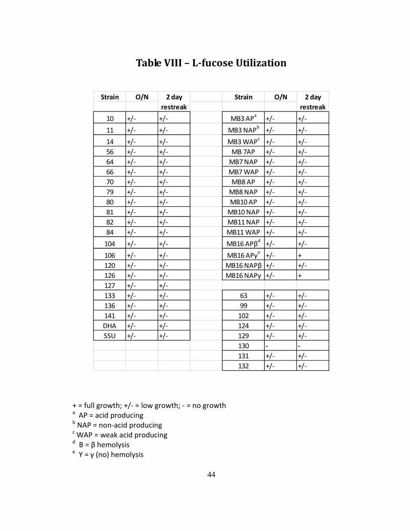
Sugar Utilization by Aeromonas strains The majority of strains were capable of utilizing each sugar as the sole

carbon source; however, growth was very sparse with small pinhead-sized colonies

(Tables VI, VII, and VIII). Isolates MB7 AP and MB8 WAP were completely unable to

utilize L-arabinose, while strains 81, 106, MB8 AP, and MB10 NAP produced some

growth when subcultured. Specific metabolic variants of A. caviae (MB3 AP, MB7

NAP, MB10 AP, MB16 APβ, and MB16 APγ) proved to be the most capable at

utilizing arabinose. The majority of strains were also capable of utilizing lactose as

the sole carbon source, including even all of the non-acid producing MB variants

included in the study. 8WAP was the only isolate that was unable to grow even

when given additional incubation time. A. caviae strains 63, 99, 102, 124, 129, 130,

131, and 132 (DNA HG 4, 5a, and 5b) were included in order to better characterize

the ability of the species to utilize L-fucose. With the exception of strain 130, all

strains were able to grow minimally on the L-fucose utilization medium. MB16 APγ

and MB16 NAPγ were able to grow relatively well after subculturing at 2 days.

FAFLP

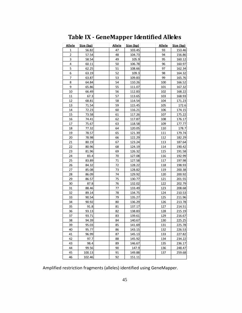
Following GeneMapper (version 3.7) analysis, a total of 137 restriction

fragments (alleles) were identified for fingerprinting (Table IX). Two separate

38

genomic DNA samples were isolated and run for each strain, and each sample was

scored independently for the presence or absence of each allele. The resulting data

was analyzed by the DendroUPGMA program (Garcia-Vallve et al., 1999) and

Dendroscope (Huson et al. 2007) was used to visualize the trees (Figure 3 and Figure

4).

Both sets of samples presented with three main clusters: a cluster of

arabinose negative A. hydrophila, a cluster of MB3 and MB7 strains, and a cluster of

A. caviae strains. A. hydrophila subsp. dhakensis was found to lie within the

arabinose negative A. hydrophila cluster in both sets of data. The closest neighbors

were found to be strains 70, 80, 106, 126, and 127 (arabinose negative A.

hydrophila).

The A. caviae metabolic variants arising from strains MB3 and MB7 were

found to cluster independently, separate of the other A. caviae strains included in

the study. Variants derived from parent strains MB8, MB10, MB11 and MB16B and

MB16Y were found to cluster indistinctly with A. caviae isolates identified as

belonging to HG groups (genomospecies) 4, 5a, and 5b.

39

Table III – A. caviae Activity on MacConkey Agar

Strain # Location isolated Source

(n = 24) O/N >4 days

22 USA/MD fecal NAPa

NAP

44 USA/MD blood NAP NAP

63 USA/DC fecal APb

AP

97 Sudan fecal NAP WAPc

99 Sudan fecal WAP WAP

102 Sudan well water NAP NAP

132 Sudan fecal NAP NAP

116 Somalia fecal NAP WAP

124 Somalia rectal NAP NAP

129 Somalia fecal WAP WAP

130 Somalia fecal NAP NAP

131 Somalia fecal WAP WAP

8 Jakarta fecal low growth WAP

137 Egypt/Cairo fecal low growth WAP

140 Sudan well water low growth WAP

12 Somalia fecal No growth No growth


6 USA/NY blood No growth No growth

34 USA/MD fecal No growth No growth

38 USA/MD fecal No growth No growth

54 USA/MD horse/foot No growth No growth


134 Egypt/Cairo water tank No growth No growth

156 Bangladesh fecal No growth No growth

MacConkey

Strains are organized by their origin of isolation. a NAP = non-acid production

b AP = acid production

c WAP = weak acid production

40

Table IV – A. caviae Tissue Cell Invasion and Cell

Associationa

Strain APb Invasion NAP

c Invasion AP Ca

dNAP CA

MB3 Trial 1 0 0 1.99E+07 4.80E+06

Trial 2 1.85E+06 N/Ae

1.67E+07 N/A

Trial 3 1.30E+06 N/A 1.39E+07 N/A

MB10 Trial 1 2.00E+05 1.70E+05 1.32E+07 3.97E+07

Trial 2 6.70E+05 1.20E+05 1.37E+07 1.87E+07

Trial 3 5.50E+05 0 1.71E+07 1.13E+07

a Initial inoculum for each well was 1 x 10

8 for a MOI of 100:1

b AP = acid producing

c NAP = non-acid producing

d CA = cell association

e N/A = experiments were not conducted

41

Table V – ONPG Hydrolysis

Strain Isolate 5 hr 48 hrMB3 APa + +

WAPb + +

NAPc N/A (clear) +

MB7 AP + +WAP N/A (clear) +NAP + +

MB8 AP + +WAP N/A (clear) +NAP + +

MB10 AP + +NAP + +

MB11 WAP N/A (clear) +NAP + +

MB16 AP-γd + +NAP-γ + +

AP-βe + +NAP-β N/A (clear) +

+ = visible yellow product a AP = acid producing

b WAP = weak acid producing

c NAP = non-acid producing

d Y = γ (no) hemolysis

e B = β hemolysis

42

Table VI – L-arabinose Utilization

Strain O/N Strain O/N

1 +/- +/- MB3 APa

+ +

10 +/- +/- MB3 NAPb

+/- +/-

11 +/- +/- MB3 WAPc

+/- +/-

14 +/- +/- MB 7AP - -

56 +/- +/- MB7 NAP + +/-

64 +/- +/- MB7 WAP +/- +/-

66 +/- +/- MB8 AP - +/-

70 +/- +/- MB8 NAP +/- +/-

79 +/- +/- MB8 WAP - -

80 +/- +/- MB10 AP + +

81 - +/- MB10 NAP - +/-

82 +/- +/- MB11 NAP +/- +/-

84 +/- +/- MB11 WAP +/- +/-

104 +/- +/- MB16 APβd

+ +

106 - +/- MB16 APγe

+ +

120 +/- +/- MB16 NAPβ +/- +/-

126 +/- +/- MB16 NAPγ +/- +/-

127 +/- +/-

133 +/- +/-

136 +/- +/-

141 +/- +/-

DHA +/- +/-

SSU +/- +/-

2 day

restreak

2 day

restreak

+ = full growth; +/- = low growth; - = no growth a AP = acid producing



d B = β hemolysis

e Y = γ (no) hemolysis

43

Table VII –Lactose Utilization


1 + + MB3 APa

+ +/-

10 +/- +/- MB3 NAPb

+ +/-

11 +/- +/- MB3 WAPc

+ +/-

14 +/- +/- MB 7AP - +

56 +/- +/- MB7 NAP + +

64 +/- +/- MB7 WAP + +

66 +/- +/- MB8 AP - +

70 +/- +/- MB8 NAP + +

79 +/- +/- MB8 WAP - -

80 +/- +/- MB10 AP + +

81 +/- +/- MB10 NAP +/- +

82 +/- +/- MB11 NAP + +

84 +/- +/- MB11 WAP + +

104 +/- +/- MB16 APβd

+ +

106 - +/- MB16 APγe

+ +

120 +/- +/- MB16 NAPβ + +

126 +/- +/- MB16 NAPγ + +

127 +/- +/-

133 +/- +/-

136 +/- +/-

144 +/- +/-

DHA +/- +/-

SSU +/- +/-

2 day

restreak

2 day

restreak




d B = β hemolysis


44

Table VIII – L-fucose Utilization


10 +/- +/- MB3 APa

+/- +/-

11 +/- +/- MB3 NAPb

+/- +/-

14 +/- +/- MB3 WAPc

+/- +/-

56 +/- +/- MB 7AP +/- +/-

64 +/- +/- MB7 NAP +/- +/-

66 +/- +/- MB7 WAP +/- +/-

70 +/- +/- MB8 AP +/- +/-

79 +/- +/- MB8 NAP +/- +/-

80 +/- +/- MB10 AP +/- +/-

81 +/- +/- MB10 NAP +/- +/-

82 +/- +/- MB11 NAP +/- +/-

84 +/- +/- MB11 WAP +/- +/-

104 +/- +/- MB16 APβd

+/- +/-

106 +/- +/- MB16 APγe

+/- +

120 +/- +/- MB16 NAPβ +/- +/-

126 +/- +/- MB16 NAPγ +/- +

127 +/- +/-

133 +/- +/- 63 +/- +/-

136 +/- +/- 99 +/- +/-

141 +/- +/- 102 +/- +/-

DHA +/- +/- 124 +/- +/-

SSU +/- +/- 129 +/- +/-

130 - -

131 +/- +/-

132 +/- +/-

2 day

restreak

2 day

restreak




d B = β hemolysis


45

Table IX - GeneMapper Identified Alleles

Allele Size (bp) Allele Size (bp) Allele Size (bp)

1 56.82 47 103.45 93 153.46

2 57.54 48 104.73 94 156.86

3 58.54 49 105.9 95 160.12

4 60.11 50 106.78 96 160.97

5 62.25 51 108.66 97 162.34

6 63.19 52 109.3 98 164.32

7 63.87 53 109.83 99 165.76

8 64.84 54 110.26 100 166.52

9 65.86 55 111.07 101 167.32

10 66.49 56 112.83 102 168.22

11 67.3 57 113.65 103 168.93

12 68.81 58 114.54 104 171.23

13 71.54 59 115.45 105 172.6

14 72.23 60 116.21 106 174.15

15 73.58 61 117.26 107 175.22

16 74.41 62 117.87 108 176.17

17 75.67 63 118.58 109 177.77

18 77.32 64 120.05 110 178.7

19 78.57 65 121.39 111 179.74

20 78.98 66 122.29 112 182.29

21 80.19 67 123.24 113 187.64

22 80.96 68 124.19 114 190.42

23 81.96 69 126.32 115 191.58

24 83.4 70 127.08 116 192.99

25 83.89 71 127.58 117 197.98

26 84.32 72 128.22 118 198.93

27 85.08 73 128.82 119 200.38

28 86.09 74 129.92 120 200.92

29 86.57 75 130.77 121 201.55

30 87.8 76 132.02 122 202.79

31 88.46 77 133.49 123 208.68

32 89.14 78 134.75 124 210.53

33 90.54 79 135.27 125 211.96

34 90.92 80 136.29 126 213.78

35 91.8 81 137.17 127 214.51

36 93.13 82 138.83 128 215.19

37 93.71 83 139.61 129 216.67

38 94.39 84 140.67 130 225.25

39 95.03 85 141.69 131 225.78

40 95.77 86 143.15 132 226.53

41 96.99 87 145.13 133 227.82

42 97.7 88 145.92 134 234.22

43 98.4 89 146.67 135 236.17

44 99.56 90 147.9 136 248.47

45 100.13 91 149.88 137 259.68

46 102.46 92 151.11 Amplified restriction fragments (alleles) identified using GeneMapper.

46

Figure I – Confirmation of DNA Stock Concentrations

Determining the concentrations of genomic DNA stocks. Each lane is labeled with

the corresponding strain’s genomic DNA stock. The three ladder lanes contain

Bioline HyperLadder I (200 - 10,000 bp).

47

Figure II – Confirmation of Digestion Procedure

Confirmation of the viability of the digestion conditions. Strains 3, 12, and 139 were

run in lanes 2, 3, and 4 respectively. Lanes 1 and 5 contain Bioline HyperLadder I

(200 - 10,000 bp).

48

Figure III – Sample A Dendrogram

Dendrogram constructed using UPGMA with Pearson’s Correlation Coefficient (r).

Distance values were calculated using the formula: d = (1 - r) * 100. Samples in

green are arabinose negative isolates of A. hdyrophila; independently clustering

variants of A. caviae are in red; strains in blue are various A. caviae; strains in black

are various nonrelated reference strains of Aeromonas.

49

Figure IV – Sample B Dendrogram

Dendrogram constructed using UPGMA with Pearson’s Correlation Coefficient (r).

Distance values were calculated using the formula: d = (1 - r) * 100. Samples in

green are arabinose negative isolates of A. hdyrophila; independently clustering

variants of A. caviae are in red; strains in blue are various A. caviae; strains in black

are various nonrelated reference strains of Aeromonas.

50

DISCUSSION

A. caviae Variant Identification

The phenospecies A. caviae includes organisms belonging to hybridization

groups (genomospecies) 4, 5A, and 5B. While some environmental isolates are

capable of producing acid from lactose utilization, others are not. The metabolic

variants in this study were originally isolated from pure non-lactose fermenting

cultures that were streaked on MacConkey agar (MAC), incubated at 37oC overnight,

and were left at room temperature for 4 days. After 4 days, it was discovered that

each plate contained discrete acid producing (AP) colonies as well as the expected

non-acid producing (NAP) colonies.

It is suggested that the production and accumulation of acidic products by AP

colonies may reduce the rate of growth, resulting in smaller colonies when

compared to NAP. The distinction between acid production from lactose and lactose

fermentation should also be noted. It is possible to produce acidic metabolites from

oxidative methods of metabolism rather than by fermentation (ex. Neisseria spp.;

Knapp and Rice, 1995). In this study, the exact metabolic differences between AP

and NAP isolates are yet unknown; therefore, the assumption that AP colonies are

capable of lactose fermentation cannot be made.

51

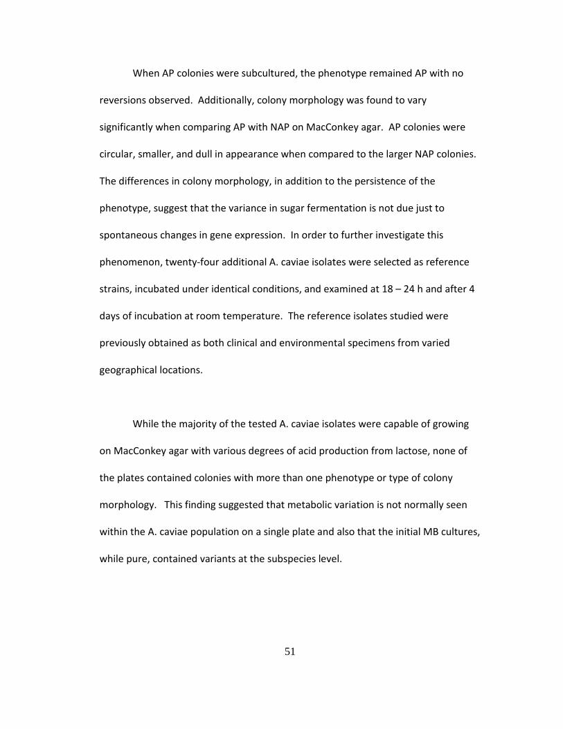
When AP colonies were subcultured, the phenotype remained AP with no

reversions observed. Additionally, colony morphology was found to vary

significantly when comparing AP with NAP on MacConkey agar. AP colonies were

circular, smaller, and dull in appearance when compared to the larger NAP colonies.

The differences in colony morphology, in addition to the persistence of the

phenotype, suggest that the variance in sugar fermentation is not due just to

spontaneous changes in gene expression. In order to further investigate this

phenomenon, twenty-four additional A. caviae isolates were selected as reference

strains, incubated under identical conditions, and examined at 18 – 24 h and after 4

days of incubation at room temperature. The reference isolates studied were

previously obtained as both clinical and environmental specimens from varied

geographical locations.

While the majority of the tested A. caviae isolates were capable of growing

on MacConkey agar with various degrees of acid production from lactose, none of

the plates contained colonies with more than one phenotype or type of colony

morphology. This finding suggested that metabolic variation is not normally seen

within the A. caviae population on a single plate and also that the initial MB cultures,

while pure, contained variants at the subspecies level.

52

It was surprising that nine isolates (6, 12, 34, 38, 54, 115, 125, 134, and 156)

produced no growth on MacConkey agar; these nine strains also grew poorly on BHI.

The isolates belonged to a variety of DNA hybridization groups (4, 5a, and 5b),

suggesting that the issue was not restricted to a group of closely related strains.

Freezer stocks for these isolates were made approximately twenty years ago, so it is

possible that the stocks were weakened following long term storage at -80oC.

Additionally, depending on the strain of A. caviae, growth on differential medium

can be significantly hindered when compared to growth on a nonselective medium

such as blood agar or BHI (Desmond and Janda, 1986). It is plausible that the

combination of poor growth on BHI and the subsequent subculture onto a selective

medium resulted in no noticeable growth.

Tissue Cell Invasion

It has been shown in Salmonella spp. (Bacci et al. 2006) that differences in

metabolic capability between species can reflect differences in their virulence

capabilities. Therefore, it was of interest whether differences in acid production

from lactose would similarly reflect a difference in virulence between AP and NAP A.

caviae strains. A quantifiable measure of the ability of A. caviae to invade tissue

cells could reflect the overall virulence of the organism.

53

Aeromonas is known to possess a variety of virulence factors that could

contribute to causing disease. However, the exact mechanism used by Aeromonas

to cause intestinal tissue damage is still unknown, mainly due to lack of an animal

model that could reproduce the gastroenteric disease seen in humans (Thorley et al.

1996; Joseph and Carnahan. 2000). Other researchers have demonstrated that

different types of Aeromonas infection involve complex pathogenic mechanisms,

including invading and penetrating the intestinal epithelial monolayer (Thorley et al.

1996; Kirov 1997; Rocha-de-Souza et al. 2003)

A method for studying tissue cell invasion was first described by Mehlman et

al. in 1982 for use with E. coli; the environment of the intestinal lining was simulated

by a monolayer of HeLa cells on the bottom of a six-well plate. In the following

years, subsequent trials have shown that the method is reliable and valid as a

virulence assay for a variety of pathogenic enteric organisms, including Aeromonas

(Couto et al. 2007).

During an invasion assay, a monolayer of tissue cells (a layer of T84 cells were

used in this experiment) is exposed to a known number of pathogens and the

system is incubated for three hours to allow for invasion. After a suitable length of

time, the tissue cells are washed and treated with the antibiotic gentamicin, chosen

specifically because it is not taken up by eukaryotic cells. Any bacteria that were

54

able to invade and penetrate the cells survive the antibiotic treatment, while those

that are still free floating or adhering to the exterior of the host cells will not.

Following gentamicin treatment, the tissue cells are then lysed and the resulting cell

lysate is serially diluted and plated in order to quantify the number of bacteria that

were able to invade. This assay, however, hinges on the ability of the pathogen to

invade the host cells; the assay will not yield any useful results If the pathogen

produces cytotoxic (causing extensive damage to the intestinal epithelium) or

cytopathic (does not damage intestinal crypts or microvilli but stimulates secretion

of water and salt) effects as its primary method of pathogenesis.

Previously, Rocha-de-Souza et al. demonstrated that Aeromonas strains are

capable of adhering to both polarized and nonpolarized Caco-2 cells. More recently,

Couto et al. described an environmental isolate of A. caviae that was able to invade

Caco-2 cells within 90 minutes (it was not reported whether the Caco-2 monolayer

was polarized or nonpolarized). Couto et al. also showed that certain strains of A.

caviae are capable of producing cytotoxic and cytopathic effects; however, they

required a minimum of 2 hours and 24 hours, respectively (Couto et al. 2007).

The limited results obtained thus far (Table IV) suggest that at 3 hours,

invasion does still occur despite the potential production of cytotoxin. It is

interesting to note that with isolate MB10, there does not seem to be a large

55

difference in invasive ability between AP and NAP isolates, while there appear to be

more significant differences in adhesion between the two metabolic variants of

MB3.

For further investigation, more strains must be studied. The current data

confirms that A. caviae is capable of invading T84 tissue cells; however, it is still

unclear whether or not there is a significant difference in invasion and adhesion

ability between acid producing and non-acid producing variants. The experiments in

this study were performed at an MOI of 100:1 based on suggested numbers of

aeromonads by Couto et al.; however, additional trials should be run to confirm that

it is appropriate (countable number of colonies on dilution plates) for A. caviae. It is

also important to conduct invasion assays with varied incubation times between 90

minutes and 3 hours to confirm that the invasion results are occurring

independently of any cytotoxic or cytopathic effects. Finally, it would also be

interesting to study another potential aspect of virulence by conducting cytotoxic

assays to assess cytotoxin production.


ONPG and Lactose Utilization by A. caviae Strains Ortho-Nitrophenyl-β-galactoside (ONPG) is a colorimetric substrate used to

detect β-galactosidase activity. β-galactosidase is required for lactose utilization,

56

and if the enzyme is present, it hydrolyzes the normally colorless ONPG molecule

into galactose and ortho-nitrophenol. Ortho-nitrophenol has a yellow color that is

visible to the naked eye, and the intensity of the color produced can be used as a

measure of the enzymatic rate. ONPG mimics lactose and is hydrolyzed by β-

galactosidase; however, it does not induce expression of the lac operon. Therefore,

organisms must be cultured on lactose rich media prior to ONPG testing in order for

β-galactosidase to be transcribed. When the MB isolates were assayed for β–

galactosidase activity using the ONPG disk assay (Table VII), all samples tested

positive, indicating that the isolates possessed β-galactosidase as reflected by their

ability to cleave ONPG.

In order for Aeromonas to utilize lactose, it must be transported across the

cell membrane by lactose permease before β-galactosidase hydrolyzes the lactose

molecule to glucose and galactose. By contrast, the ONPG reagent is able to diffuse

through the membrane without the aid of a transporter. It was very surprising to

note that, while growth was minimal, all of the non-acid producing MB variants in

the study were capable of utilizing lactose as the sole carbon source for growth.

Therefore, the ONPG results (Table VII) suggest that the NAP isolates are deficient in

a step in lactose metabolism prior to β-galactosidase, namely lactose permease. It

was interesting to note that the MB variants also appeared to be capable of utilizing

57

L-arabinose and L-fucose; however, there did not appear to be significant

differences in the ability to utilize the two sugars between AP and NAP variants.

On MAC, organisms that are incapable of utilizing lactose are able to break

down peptone instead; however, the lactose utilization minimal media contains no

other carbon source except lactose. In order to discount the possibility that growth

was occurring using endogenous metabolites remaining from the rich media (BHI)

used to revive the strains from freezer stock, samples were subcultured following 2

day incubation on the sugar utilization medium. Growth was observed after

subculturing; however, there appeared to be variations in colony size between AP

and NAP cultures. At this point, while there are clear metabolic differences between

AP and NAP isolates, the exact mechanism causing these differences is still

unknown.

Future work should examine the possibility that lactose permease might be

deficient but still functional in NAP isolates. In the current study, lactose utilization

plates were examined at 24 h intervals and scored for growth. However, the exact

amount of growth was only generally classified: growth (+), low growth (+/-), and no

growth (-). Additional attention must be given to the colony size, morphology, and

speed of growth; if NAP presents with smaller or slower growing colonies when

58

compared to AP isolates, this may suggest a deficient rather than inactivated lactose

permease.

Sugar Utilization by A. hydrophila strains

In order to characterize the new subspecies A. hydrophila subsp. dhakensis,

Huys et al. analyzed 152 phenotypic characteristics; it was found that eight specific

tests: utilization of L-arabinose, L-fucose, methyl a-d-mannoside, urocanic acid, cis-

aconitate, DL-aspartate, caprate, and acid production from L-arabinose, could be

used to distinguish A. hydrophila subsp. dhakensis from DNA HG 1 A. hydrophila

(Huys et al. 2002). Previous work with a large group of HG 1 A. hydrophila

corroborated the results obtained by Huys et al. from the utilization of L-arabinose,

utilization of urocanic acid, and production of acid from L-arabinose (Abbott et al.

1992; Hänninen 1994; Kämpfer and Altwegg 1992), therefore, it was suggested that

these three tests be considered the major differential tests used for the

identification of the subspecies dhakensis. A. hydrophila subsp. dhakensis was

defined as unable to utilize L-arabinose, non-acid producing on L-arabinose, and able

to utilize urocanic acid as its sole carbon source.

Previous work by Carnahan and Joseph had described a genotypically distinct

group of arabinose negative A. hydrophila, which like A. hydrophila subsp. dhakensis,

did not produce acid from L-arabinose (Carnahan and Joseph 1993). It was

suspected that these strains potentially belonged to the subspecies dhakensis;

59

therefore, a panel of arabinose negative A. hydrophila isolates was cultured on the

L-arabinose and also an L-fucose utilization medium. Like with the lactose utilization

assay described above, samples were subcultured following 2 days of incubation on

the sugar utilization medium to discount the possibility that growth was occurring

using endogenous metabolites remaining from BHI used to revive the samples from

freezer stock.

Huys et al. and Martinez-Murcia et al. had found that A. hydrophila subsp.

dhakensis was incapable of utilizing L-arabinose. Thus, it was contrary to

expectations that all arabinose negative (non-acid producing) isolates (strains 10, 11,

14, 56, 64, 66, 70, 79, 80, 81, 82, 84, 104, 106, 120, 126, 127, 133, 136, 141, and

dhakensis) were able to grow on the minimal media and grew at approximately the

same rate as the arabinose positive (acid producing) type strain of A. hydrophila

(strain 1). Urocanic acid was unavailable for this study; therefore, utilization of L-

fucose was included instead. Huys et al. found A. hydrophila subsp. dhakensis to be

incapable of L-fucose utilization, but again, it was surprising to note that all

arabinose negative strains in this experiment (including subsp. dhakensis) were able

to grow on minimal L-fucose media. Finally, the arabinose negative strains were also

streaked onto excess lactose utilization media from earlier experiments. It was

interesting to observe that HG 1 A. hydrophila grew quite well on this medium, while

arabinose negative isolates were only capable of minimal growth.

60

It is difficult to explain how results from this study seemingly contradict

published results. A possible explanation may lie in a difference of methodology;

the sugar utilization protocol used in this study was obtained from a collaborator

with Dr. Martinez-Murcia rather than from the laboratory of Dr. Huys. Additionally,

growth was generally minimal and so plates were generally incubated for 48 hours

before observation. The presence of small pinhead colonies by 48 hours, while

minimal, was still scored as a positive test and the isolate was considered able to

utilize the sugar. Huys et al. also did not specify when (following how long of an

incubation) and how they scored growth (presence/absence or if amount of growth

was taken into account). At the present, it is unknown if the two sets of data are

comparable and additional trials must be completed with these strains under more

standardized conditions for concrete conclusions to be drawn.

If additional L-fucose and L-arabinose utilization data continues to prove

inconclusive, previous work by Joseph and Carnahan suggest additional phenotypic

tests that may aid in the identification of additional “dhakensis” strains. Arabinose

negative strains, like subsp. dhakensis, were found to have a greater frequency of

acid produced from salicin, greater resistance to ceftazidime, imipenem, and

cefoxitin when compared to arabininose positive strains. These assays have yet to

be used to compare “dhakensis” with arabinose positive A. hydrophila and may add

61

to the panel of tests first described by Huys et al. for the identification of subsp.

dhakensis.

FAFLP

In the past, DNA/DNA hybridization was considered the gold standard for

species classification in Aeromonas taxonomy. Due to repeatability issues (high

variability with results) and the complexity of the protocol, replacement techniques

and approaches have been sought. FAFLP was chosen for this study over other

molecular techniques for its appropriate resolution and reproducibility: random

amplification of polymorphic DNA (RAPD) analysis has a high amount of variability

even within a subspecies, and pulsed-field gel electrophoresis was found to lack

resolution past the species level (Huys et al. 1996). Ribosomal DNA sequence

polymorphisms (ribotyping) or 16s rRNA restriction fragment analysis are also

limited in their sensitivity due to lower number of bands available for analysis when

compared to AFLP.

The laboratory of Dr. David Hawthorne (UMCP) regularly performs FAFLP

experiments and graciously shared their FAFLP protocol; however, samples were

analyzed on the ABI 3730xl DNA sequencer using the Fragment_analysis_D module

instead of the AFLP_Long module suggested by the Hawthorne protocol. When

Fragment_analysis_D was compared to the AFLP_Long module, there were only a

few minor changes: 1.5 injection voltage instead of the AFLP_Long 1.6, 180 for 1st

62

and 2nd readout time instead of 200 (described in the manual as the interval of time

for data points to be produced), 5 for current stability instead of 3 (ABI default

setting was 5 ; current stability is the maximum allowed current variation, anything

greater is attributed to bubbles in the sample and causes an abort), and most

importantly, 1700 instead of 3000 seconds for run length.

Based on the 3730xl instruction manual, the differences in the run modules

are negligible except for the adjustment to the run length. The Hawthorne lab

suggested the longer 3000 second run time to allow for better separation of larger

pieces (up to 1 kb in length). By comparison, this study utilizes AFLP to look at

Aeromonas isolates. Due to the genome size and restriction enzymes used, shorter

fragments approximately 35-500 bp in length are produced. While the AFLP_Long

module could theoretically be used, running things for a longer period results in

distortion of the spacing between smaller fragments (< 100 bp in size) and as a

result, the long run length was not ideal for this study.

In order to create dendrograms for genotypic analysis, the un-weighted pair

group method with arithmetic mean (UPGMA) was used with 100 bootstrap

replicates. The tree was created with the reference strains from Table I in order to

help visualize the relationship among the metabolic variants; the bootstrap

replicates were conducted as part of the analysis to test the tree’s reliability. The

63

algorithm analyzes the amplified fragment matrix when constructing a rooted tree;

at each step, the nearest two clusters are combined into a higher-level cluster.

Pearson’s correlation coefficient is used as part of the algorithm to measure the

degree of association (positive or negative) between each strain.

UPGMA was chosen for this study due to its relative ease of use, and in order

to confirm the results of Huys et al. 2002, who also used this method to propose A.

hydrophila subsp. dhakensis as a new subspecies. It should be recognized that this

method of analysis assumes a constant rate of nucleotide substitution throughout

the evolutionary history of the taxa, which may not be applicable for all cases. As a

result, for more detailed phylogenetic work, UPGMA is used to produce guide trees

prior to more sophisticated phylogenetic algorithms; in this case, UPGMA provides

enough resolution to draw conclusions at the subspecies level.

While FAFLP results have been shown to be highly reproducible (Janssen et

al. 1996; Huys et al. 1996), there were differences in the dendrograms produced by

the two trials. Despite the differences in the exact order, all of the MB3 and MB7

isolates clustered together, with no close neighbors. The remaining MB8, MB10,

MB11 and MB16 isolates clustered together with 3, 12, 115, 137, 139, 140 (A. caviae

DNA HG 4, 5a, 5b) and A. hydrophila subsp. dhakensis clustered closely with 70, 80,

106, 126, and 127 (arabinose- A. hydrophila). When comparing MB3/MB7 cluster,

64

the evolutionary distances (31.37 for sample A, 28.76 for sample B) were

significantly less than the distances between species A. hydrophila, A. veronii, and A.

trota (each of which was equal or greater to 41.5 for both trials). While there is not

enough evolutionary distance to be considered a new species, the separate

clustering suggests that MB3 and MB7 may belong to their own subgroup of A.

caviae. Additional differential metabolic testing to identify a unique metabolic

profile must be performed before this subgroup can be defined as a new subspecies.

With regards to A. hydrophila subsp. dhakensis, the results seem to validate

the work by Huys et al.; the arabinose negative strains of A. hydrophila are relatively

distinct from the arabinose positive strains of A. hydrophila HG 1. Additionally, the

arabinose negative strains tended to be relatively equidistant from each other with

no tight clustering within the group. However, these strains, while evolutionarily

distinct from HG 1, are more related with slightly smaller distance values (37.9 for A,

37.0 for B) than the values generated for distinct species of Aeromonas (>= 41.5).

This suggests that the original proposal to classify these strains as a subspecies

rather than species based on FAFLP results was conservative, but if additional

genetic or phenotypic differences were reported, it could lead to a bolder

classification as the novel species A. dhakensis.

65

Conclusions

While the metabolic data remains inconclusive, the FAFLP results do suggest

that MB3 and MB7 may belong to a new subspecies of A. caviae; MB 8, MB10,

MB11, MB16, and MB16 appear to belong to groups previously established through

DNA-DNA hybridization. It is interesting to note that it was hypothesized that there

would be differences between A. caviae metabolic variants; however, it appears that

two out of the seven original strains potentially belong to their own subspecies

instead. The exact mechanism for the differences in acid production from lactose

remains unclear, as the phenomenon cannot be explained solely through variability

in gene expression. Additional studies to further characterize the MB3 and MB7

variants, including metabolic and virulence assays, must be performed prior to

defining the cluster as a new subspecies of A. caviae.

Similarly, A. hydrophila subsp. dhakensis does appear to be properly

classified, at least via FAFLP, as a subspecies of A. hydrophila rather than a new

species of Aeromonas. Future studies may suggest additional differences between

subsp. dhakensis and HG 1 Aeromonas that may lead to a reclassification; however,

the precedent in that case would be to elevate subsp. dhakensis to a novel species

rather than the use of A. aquariorum, as has been championed by Martinez-Murcia

et al. (Martinez-Murcia et al. 2008a)

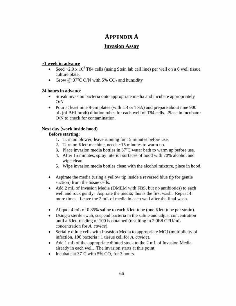
66

APPENDIX A

Invasion Assay

~1 week in advance

• Seed ~2.0 x 105 T84 cells (using Stein lab cell line) per well on a 6 well tissue culture plate.

• Grow @ 37oC O/N with 5% CO2 and humidity

24 hours in advance • Streak invasion bacteria onto appropriate media and incubate appropriately

O/N • Pour at least nine 9-cm plates (with LB or TSA) and prepare about nine 900

uL (of BHI broth) dilution tubes for each well of T84 cells. Place in incubator O/N to check for contamination.

Next day (work inside hood)

Before starting: 1. Turn on blower; leave running for 15 minutes before use. 2. Turn on Klett machine, needs ~15 minutes to warm up. 3. Place invasion media bottles in 37oC water bath to warm up before use. 4. After 15 minutes, spray interior surfaces of hood with 70% alcohol and

wipe clean. 5. Wipe invasion media bottles clean with the alcohol mixture, place in hood.

• Aspirate the media (using a yellow tip inside a reversed blue tip for gentle

suction) from the tissue cells. • Add 2 mL of Invasion Media (DMEM with FBS, but no antibiotics) to each

well and rock gently. Aspirate the media; this is the first wash. Repeat 4 more times. Leave the 2 mL of media in each well after the final wash.

• Aliquot 4 mL of 0.85% saline to each Klett tube (one Klett tube per strain). • Using a sterile swab, suspend bacteria in the saline and adjust concentration

until a Klett reading of 100 is obtained (resulting in 2.0E8 CFU/mL concentration for A. caviae)

• Serially dilute cells with Invasion Media to appropriate MOI (multiplicity of infection, 100 bacteria : 1 tissue cell for A. caviae).

• Add 1 mL of the appropriate diluted stock to the 2 mL of Invasion Media already in each well. The invasion starts at this point.

• Incubate at 37oC with 5% CO2 for 3 hours.

67

Following invasion (work outside of hood) • After 3 hours, aspirate media (as described above) from the invasion wells

only. • Add 1 mL 200 ug/mL gentamicin in DMEM culture media and 2 mL of

Invasion Media to each invasion well. This step does not apply to the cell-associated wells.

• For cell-associated wells, add 3 mL of invasion media. • Incubate for 2 h at 37oC with 5% CO2 to allow the gentamicin to kill all cell

surface attached bacteria. • Take 1 mL of the media from each invasion well and plate 100 uL to ensure

that there are no surviving free floating bacteria in the “supernatant”. • Wash each well 5x with 1x PBS (as described above with Invasion Media);

aspirate the remaining wash from each well. • Add 1 ml of 0.1% Triton X to each well to lyse the tissue cells. • Incubate at 37oC with 5% CO2 for 15 minutes to allow the Triton X to work.

• Use a cell scraper to loosen and concentrate the lysate as much as possible.

Using a micropipet, transfer the cell lysate from each well into a separate microcentrifuge tube. Pipet the solution in the tube up and down 20x to break up any cell clumps.

• Make 10-3 through 10-5 dilutions of the cell lysates, and pipet 100 uL of each dilution onto plates and spread.

• Incubate at 37oC with 5% CO2 O/N. Count bacterial colonies the next day.

68

APPENDIX B

ONPG Disk Detection for Presence of β-Galactosidase BD BBL Taxo ONPG disks – VWR catalog #90002-222

Objective: This test is used to demonstrate the presence or absence of the enzymes β-galactosidase and lactose permease using the substrate ortho-nitrophenyl-β-D-galactopyranoside (ONPG). Since the enzymes are induced in the presence of lactose, the organism to be tested should be grown on media high in lactose (lactose broth) for best results (according to manufacturer’s instructions). Reagents: ONPG disks (store refrigerated between -20 and 8oC) Sterile saline (or TSB, 0.5 mL for each sample to be tested) Sterile small test tubes 10 µL bacteriology loop Sterile graduated Pasteur pipette Procedure: 24 hours prior

1. Streak the organisms to be tested on TSI agar. Incubate overnight at appropriate growing conditions

For each sample to be tested

1. Place an ONPG disk into a sterile tube and add 0.5 mL sterile saline or TSB. 2. Heavily inoculate the tube with a loopful of the test isolate. A heavy

inoculum is necessary to obtain a high concentration of enzyme. 3. Incubate at 35oC for 4 to 6 hours.

Controls

Positive: E. coli (ATCC 25922) Negative: M. morganii (ATCC 8019)

Interpretation • Positive for β-galactosidase: yellow color within 4-6 hours or following O/N

incubation. • If colorless at 4 hours, incubate O/N before discarding as negative for β-

galactosidase

69

APPENDIX C

Carbohydrate Utilization Media

Objective: This differential minimal media is used to test for carbohydrate utilization. Reagents (1L): 15 g agar (Difco) 2 g of the appropriate carbohydrate carbon source (ex: L-arabinose, L-fucose, or lactose) 6.1 g Tris-HCl pH 7.5 (50mM) 1 g NH4Cl 75 mg K2HPO4

28 mg FeSO4-7H2O Ultra-pure water (Milli-Q) to 1L. Procedure: 1. Prepare plates using 20 mL of agar per plate.

2. Isolates to be tested should be streaked onto the hardened agar.

3. Incubate plates at 37oC for 24 h.

4. If no growth was observed O/N, incubate for another 24 h.

5. At 2 days, subculture each plate to confirm initial observation.

Interpretation Growth on the medium signifies the ability to utilize the sugar.

70

APPENDIX D

FAFLP Procedure

DAY 0 Grow strains O/N in 5 mL of the appropriate liquid growth media. DAY 1 - Isolation of DNA Isolate genomic DNA via CTAB Isolation:

1. Spin 2 mL liquid culture in a 2 mL centrifuge tube for 2 min at max speed in a microcentrifuge. Discard supernatant, resuspend pellet in another 2 mL liquid culture, repeat the centrifugation, and discard the supernatant. Spin a final time for 30 sec to remove as much liquid as possible.

2. Resuspend pellet in 567 µL TE buffer, then add 30 µL 10% SDS and 3 µL 20mg/mL proteinase K (final concentration is 100 µg/mL proteinase K in 0.5% SDS) to lyse the cells. After mixing thoroughly, incubate for 1.5 h at 37oC.

3. Add 100 µL 5M NaCl warmed to 65oC, mix thoroughly.

4. Add 80 µL CTAB/NaCl solution warmed to 65oC, mix and incubate for 10 min at 65oC.

5. Add 0.75 mL chloroform/isoamyl alcohol, mix, and spin for 10 min at max speed in a microcentrifuge.

6. Remove a total of 600 µL (200 µL three times to minimize loss of pellet) supernatant into a fresh microcentrifuge tube, add 3 µL RNaseA and incubate for 1 h at 37oC.

7. Add 600 µL 25:24:1 phenol/chloroform/isoamyl alcohol, mix, and spin at max speed for 10 min.

8. Transfer another 600 µL (200 µL three times) supernatant to a fresh tube, add 390 µL (0.6 volumes) isopropanol to precipitate the DNA. Do not vortex.

9. Spin DNA for 5 min at max speed, discard supernatant, tap rim of tube on a kimwipe to blot.

10. Resuspend with 100 µL 70% ethanol to wash DNA, vortex, respin DNA for 5 min. Blot excess ethanol on kimwipe as described above.

11. Dry DNA in lyophilizer for 1.5 h; redissolve in 100 µL TE Buffer.

Check quality/quantity of DNA isolated via gel electrophoresis and DNA spec. DNA stocks should be stored frozen at -20oC.

71

DAY 2 – Preparation for PCR Amplification Make AFLP templates via digestion of ~1 µg genomic DNA using ApaI and TaqI. Ligate double strand adapters (ordered as oligonucleotides), reaction mix concentrations as follows: (Janssen et al. 1996, Vos et al. 1995) 10 µL volume, added to restriction digest consisting of: 0.04 µM ApaI adaptor 0.4 µM TaqI adaptor 1 U T4 DNA-ligase 1mM ATP in 10 mM Tris-HAc pH 7.5 10 mM MgAc 50 mM KAc 5 mM DTT 50 ng/µL BSA Incubate reaction mixture for 3 h at 37oC. Post-ligation mixture diluted to 500 µL with 10 mM Tris-HCl, 0.1 mM EDTA pH 8.0, store at -20oC. DAY 3 – PCR Amplification of Fragments (resulting in 35-400 bp bands) An additional preselective amplification step is possible (PCR once with unlabeled primers) before the selective amplification; however, it was found that a one-step selective PCR amplification resulted in more bands with equal intensity to the two step amplification. PCR Mix: 1.5 µL digested template fragments 0.5 µL A01-6FAM primer 0.5 µL T01-6FAM primer 7.5 µL Amplification Core Mix PCR steps:

1. Denature at 94oC for 2 min

2. 10x cycle of: a) Denature at 94oC for 20 sec b) Anneal at [66-(n-1)] oC for 30 sec, where n = the cycle number c) Extension at 72oC for 2 min

3. 20x cycle of a) Denature at 94oC for 20 sec b) Anneal at 56oC for 30 sec c) Extension at 72oC for 2 min

4. Final extension at 60oC for 30 min

72

APPENDIX E

MODIFIED HAWTHORNE LAB PROTOCOL : AFLP SAMPLES ON THE 3730 Prepare Run File

• Enter sample names into file • Save as text tab delimited

Prepare samples for the 3730

• Prepare HiDi + TAMRA: 776µL HiDi + 24µL each of GeneScan 500 & 2500 • Aliquot 6µL HiDi + TAMRA into notched plate • Add 4µL PCR product, mixing up and down • Spin down to remove bubbles • Instant incubate on the thermocycler: 95 for 2-3 minutes, then place directly

on ice Put sample tray in 3730

• Place the sample plate in the black tray and fit the white lid over the unit. Make sure the tab clicks and the wells are visible from the top.

• Check to be sure the red light is NOT on. Open the right-side door to the 3730 by pulling it out, slide out the rack, and open the door to the stacker furthest away from the machine (or closest to you when pulling it out). Place sample plate in the stacker with the notched corner on the back right. Close the stacker door and then the ABI.

Set up and start your run

At the computer closest to the 3730, select “Plate Manager”, Import, and look the shared folder on “dfgil41 H:” • Copy the file from the flash drive (find in “My Computer”) to “Shared Data”

folder, “UploadFolder”, “Joseph Lab” • Open folder “Joseph” • Select the file, then click OK • Select “Run Scheduler”, Search, then type in your file name • Select your file, hit Add, then press Done • Press the green triangle to start the run. If the machine is already running, it

will automatically start the next run. The plate on the bottom of the stack is the next to be run.

• Fill out the Run Log

73

APPENDIX F

Abridged Hawthorne Lab GeneMapper Protocol for Analysis Modified from 05/21/10 version written by Julie Byrd Hebert

General Notes:

If you are using more than one dye: the analysis method in GeneMapper will lock

you into co-loading the same primer combinations each time. Keep this in mind

when running PCRs and loading the sequencer.

General definitions:

• Kit – a set of panels with a set of bin definitions, also called “chemistry kit”.

• Panel – within a kit, a specific set of analysis options that can be used on a

set of samples.

• Marker – a specific dye (marker) associated with a given panel.

• Bin – an area in which a peak is defined.

• Peak Size – the actual size of the peak (in base pairs (bp)), typically on the x-

axis.

• Peak Height – the fluorescence of the peak, typically on the y-axis.

1. Creating Project and Adding Samples

- Double-click on GeneMapper on the Desktop (Note: may take a while to

open)

• Username: gm

• Password: josephlab

- If not already set, choose ‘AFLP default’ in the “Table setting:” pull-down

menu

� File � Add Samples to Project (or test tube button on toolbar)

Note: you may want to change this table setting once you get used to using the

program.

- Find and select folder for desired sequencer run, or specific samples (if not

using all samples in one folder)

- Click ‘Add to List’

- When finished, click ‘Add’

- Save Project as: [date]_[primers]_[samples/plate id], or another appropriate

name that you can remember. (Ex: 090608_Eact-Paag_plate1) or open

project if you have one already created to which you need to add samples

2. Setting up Panel

- **Go to Tools � Panel Manager, click on ‘Panel Manager’ in the left-hand

frame menu, then � File � New Kit

74

- **Name your new kit [initials]_AFLP or something similarly simple and

appropriately descriptive. Only need to do this once, you can it for any

number of panels within a single kit.

- **Choose ‘Microsatellite’ as type (there is no AFLP designation)

- Click on your new kit in the left-hand frame menu

� File � New Panel

- In the right window, you will be able to name your new panel

- Name this panel AFLP_[sample descriptor] or something similarly simple Ex:

AFLP_towhees.

- Click on your new panel folder in the left-hand frame menu (this may take a

while) � File � New Marker

- Create a new marker for each labeled primer run. Change the names to the

dye color (e.g. blue)

- make sure the dye colors are denoted correctly, change size range 0-999, and

change marker repeat unit to 9, leave stutter ratio on 0.0

- Click Apply and then OK.

3. Setting up the Analysis Method

- Go to Tools � GeneMapper Manager � ‘Analysis Methods’ tab. The

following starred steps only need to be performed once.

- **Click on ‘New’ to set up a new method

- **Choose ‘AFLP’ as your analysis type

- **Name your method ‘AFLP_[initials]’, give it a description if you like, and

enter ABI 3730 in the ‘Instrument’ box.

- Go to the ‘Allele’ tab

o Panel: select ‘Generate panel using samples’

o Make sure ‘delete’ common alleles’ is not toggled on if you want to keep

monomorphic peaks.

o Under ‘Analyze Dyes’, only choose blue (unless you are using more than

one).

o Under ‘Analysis Range’ choose one above the first two bands in the

ladder and one below the two top bands.

- Go to the ‘Peak Detector’ tab

o Under ‘Peak Detection Algorithm’, select ‘Advanced’.

o Under ‘Sizing’ select ‘Partial Sizes’. Change the minimum and maximum

to match the numbers in the Analysis Range (above).

o Under ‘Smoothing’ select ‘Light’.

o Under ‘Peak Detection’ check that B = 5000, R = 75.

- Click ‘Okay’, then click ‘Done’.

4. Changing Analysis methods

- Under the Analysis method column in the Samples table

75

o Click on the first cell in this column.

o Select ‘AFLP_[initials]’ or whatever you named your method.

o Highlight the whole column by clicking on the top column � fill using

Ctrl-D

- Under the Panel column

o Leave as ‘none’ (you are creating a panel with this analysis step).

- Size Standard

o Select the appropriate size standard. If this does not exist, you will

need to create your own marker standard.

� Click on ‘New Size Standard’.

� Choose ‘Advanced’.

� Give the size standard a name (such as the names above) and

any description needed to identify the size standard.

� Make sure the dye color is correct for the size standard.

� Starting with the lowest number, enter each size standard

peak into a row.

� IMPORTANT: YOU MAY NEED TO DELETE THE PEAKS ABOVE

700 IF THE ABI IS NOT COLLECTING DATA BEYOND THAT

POINT. OTHERWISE, YOUR MARKER WILL MISMATCH AND

YOU CAN’T ANALYZE YOUR DATA.

o Highlight the whole column by clicking at the top of the column � fill

using Ctrl-D.

5. Analysis of Samples

- Click on the “play button” (the green arrow in the toolbar), all samples

should run through analysis (NOTE: this will take time, especially when it

auto-saves.)

• All of the symbols in the OS and SQ columns should be green.

- If some SQ’s are red:

• Select the sample(s) and click on the Size Match editor in the toolbar

(the button with the red peaks) Helpful hint: you might want to make

the window bigger by clicking on the corner and dragging it out.

• � Edit � Override all SQ. This will automatically accept all of the

current peaks (which is a lot easier than clicking the override button

for each sample separately).

• **Correct any mislabeled peaks (left click a peak to select, right click

to alter) for each sample, then go to the next sample.

• Once you have checked all of these samples, click ‘Ok’.

• If the size standard is too low for peaks to be called (<25 fluorescence

units), note for re-run, and then delete the sample from the project .

• Note: if this is done, the sample(s) will have to be reanalyzed .

- If some OS’s are yellow cautions:

76

• Note in the display plots which peaks are off-scale – those peaks will

not have accurate size calls, and may throw off the size calls of peaks

near them. If those size bins look useful when editing marker bins,

you will have to dilute and re-run those samples with off scale reads.

- Once all have been corrected, hit play.

- Double check the quality of your samples in the sample plot window

(multicolored peak button on the toolbar)

• Highlight the entire project; click the sample plot button.

• Toggle on any/all appropriate colors and scroll through your samples

to make sure there are none under-amplified and no samples that

look very different than all the others. If there are, note those

samples.

- Close the sample plot window.

- If there were any samples that should be deleted, click on the sample then

select

� Edit � Delete from Project.

- Once all have been corrected, hit play. You will need to make sure no “play”

symbols are present before you export your project panel.

6. Exporting Project Panel and Bins

� File � Export Project Panel

• Chemistry Kit: (use your kit name plus an additional character, e.g.

JBH_AFLP1)

• Panel Name: (use your panel name plus an additional character, e.g.

AFLP_Phytomyza1) If you haven’t named your panel yet, put

whatever you are planning to label your panel in here.

- Save to Desktop (or an appropriate folder).

7. Editing Project Panel Bins

- On Desktop, two files will have been created

• Delete the file without ‘bin’ in the name (panel file).

• Open the .txt file that does have ‘bin’ in the name.

- In the text file, change:

• Kit name: [your kit name] (e.g. SEK_AFLP).

• BinSet name: AFLP_[names]_BinSet_[whatever you name it].

� Important: the first two parts don’t matter as much, but you

must have the “_BinSet_ “.

• Panel name: [your panel name] (e.g. AFLP_towhees)

- Save and exit Text Editor

8. Importing Bins

� Tools � Panel Manager

77

-Highlight your chemistry Kit (e.g JBH_AFLP)

� File � Import Bin Set

- If you already have a bin set by that name, you will need to either rename

your new bin set, or delete the current bin set before adding your new one.

• To delete the current bin set, make sure it is selected in the

dropdown window, � Bins � Delete Bin Set.

- Select the text file that was just edited from the desktop and import

- If there are overlapping bins, you will get an error message. The error log

can be located at this pathname

C:/AppliedBiosystems/GeneMapper/PanelImportlog.txt

• Open it and note what size bins overlap.

• Open your bin .txt file on the desktop and change one of the

overlapping bin sizes by 0.01bp so they no longer overlap.

• Save and exit Text Editor.

• Repeat your import process, it should work.

- Your new binset will now be in the ‘BinSet’ pull-down menu in the Panel

Manager

- Click apply and OK

9. Sample Re-Analysis

- Return to GeneMapper window (samples table)

- Go to Analysis � Analysis Method Editor � Allele Tab

• Panel: toggle to ‘use specified panel’.

• Bin Set: select the new bin set in the pull-down menu.

• Click ‘OK’.

- Select the column ‘Panel’

• Change ‘None’ to [your panel name].

• Select entire column, fill with Ctrl-D.

- Click green arrow to reanalyze the data

- Again, correct any error in size standard (SQ), and if you do, run the analysis

again.

• (See note about correcting size standards under 5. Analysis of

Samples.)

10. Editing Marker Bins

� Tools � Panel Manager

- Highlight your panel in the left-hand frame menu.

- Double check and make sure your bin set is selected in the drop-down menu

at the top of the page.

� Bins � Add Reference Data (or the test tube button on the toolbar)

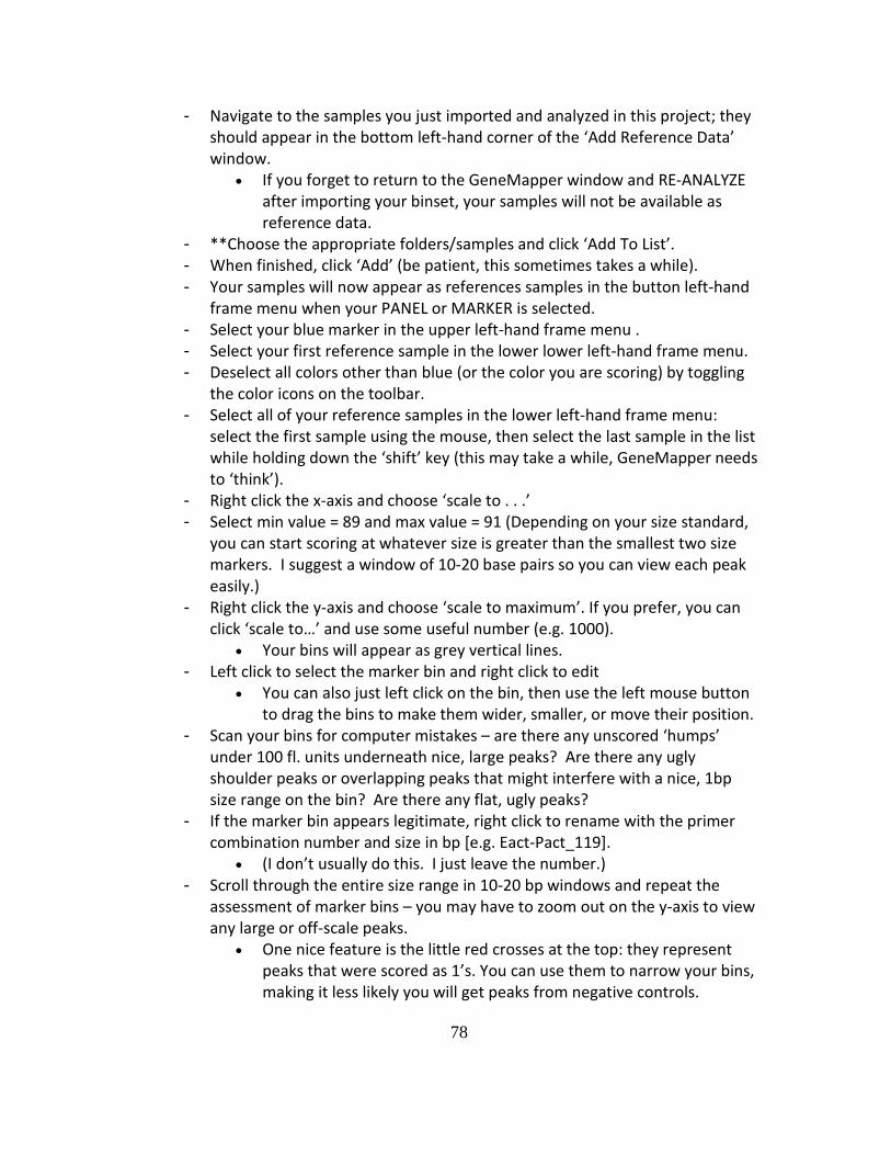
78

- Navigate to the samples you just imported and analyzed in this project; they

should appear in the bottom left-hand corner of the ‘Add Reference Data’

window.

• If you forget to return to the GeneMapper window and RE-ANALYZE

after importing your binset, your samples will not be available as

reference data.

- **Choose the appropriate folders/samples and click ‘Add To List’.

- When finished, click ‘Add’ (be patient, this sometimes takes a while).

- Your samples will now appear as references samples in the button left-hand

frame menu when your PANEL or MARKER is selected.

- Select your blue marker in the upper left-hand frame menu .

- Select your first reference sample in the lower lower left-hand frame menu.

- Deselect all colors other than blue (or the color you are scoring) by toggling

the color icons on the toolbar.

- Select all of your reference samples in the lower left-hand frame menu:

select the first sample using the mouse, then select the last sample in the list

while holding down the ‘shift’ key (this may take a while, GeneMapper needs

to ‘think’).

- Right click the x-axis and choose ‘scale to . . .’

- Select min value = 89 and max value = 91 (Depending on your size standard,

you can start scoring at whatever size is greater than the smallest two size

markers. I suggest a window of 10-20 base pairs so you can view each peak

easily.)

- Right click the y-axis and choose ‘scale to maximum’. If you prefer, you can

click ‘scale to…’ and use some useful number (e.g. 1000).

• Your bins will appear as grey vertical lines.

- Left click to select the marker bin and right click to edit

• You can also just left click on the bin, then use the left mouse button

to drag the bins to make them wider, smaller, or move their position.

- Scan your bins for computer mistakes – are there any unscored ‘humps’

under 100 fl. units underneath nice, large peaks? Are there any ugly

shoulder peaks or overlapping peaks that might interfere with a nice, 1bp

size range on the bin? Are there any flat, ugly peaks?

- If the marker bin appears legitimate, right click to rename with the primer

combination number and size in bp [e.g. Eact-Pact_119].

• (I don’t usually do this. I just leave the number.)

- Scroll through the entire size range in 10-20 bp windows and repeat the

assessment of marker bins – you may have to zoom out on the y-axis to view

any large or off-scale peaks.

• One nice feature is the little red crosses at the top: they represent

peaks that were scored as 1’s. You can use them to narrow your bins,

making it less likely you will get peaks from negative controls.

79

- Stop scoring at a size where weaker samples start to lose what otherwise

appear to be monomorphic peaks (probably 900-950bp in size). If your

samples look nice all the way up to the cut-off of the run, stop scoring before

you reach the second to largest size standard marker

- Toggle on any colors that were run concurrently and check for pull-up under

high peaks.

- Click Apply and OK to exit out of Panel Manager.

- Rerun the analysis, including overriding the ladders. If you did not edit or add

any bins, continue on to Step 11.

- If you did change or add any bins, return to the 79-91 bp window and double

check those bins.

• Again, for the bins you changed, you should be able to narrow the

bins close to the red crosses.

- Do this for the entire size range.

- Click ‘Apply’

- Repeat the scoring process for your green marker

- Export your marker bins for record/reference

• Click on the chemistry Kit, � File � Export Bin Set

• Click ‘Apply’ and OK

11. Sample Re-Analysis

- Return to GeneMapper window (samples table)

- Make sure you have selected the correct analysis, size std. and panel

- Click green arrow to reanalyze the data.

- Select only your negative controls and view them using the view button in

the tool bar. (It has a blue, red, and green peak on it.)

- Zoom in by dragging the mouse over a smaller section of one of the samples.

• If any of the negative controls have a peak, select the button on the

top left that shows a bin around a peak. (The one with grey under the

peak is the default.)

• Right click on the bin with the peak in the negative control, and delete

the bin.

- Continue checking all of the negative controls by scrolling up and down

between the samples, and left and right along the peak size.

- When you close the window, you will get a warning asking if you want to

save the Project Panel. Choose Yes.

- Correct any error in size standard (SQ). If you were not correcting your

ladders during the process above, make sure to do it now.

- Click on the ‘Genotypes’ Tab (next to the ‘Sample’ Tab).

• Your Genotypes table will now be filled with 0 and 1 scores for all

your validated bin sets.

80

• If not, go to the Table Setting Editor (the button that looks like a

table) � Genotypes � Check the Allele button in the scroll down list.

Click okay, then the alleles with 0 and 1 scores should show up in your

genotype table. You can also just change the Table Setting to “AFLP

Default.”

� File � Export Table or Ctrl-E

- Save the table in your folder on the desktop.

- Unless you have the new version of Microsoft office or you are using some

shareware with a good spreadsheet, you will likely not be able to view all of

the columns in the exported file. Therefore, you may want to make a Table

Setting with only the ‘Allele” button checked but not peak height, etc.

- Keep a separate excel file of all samples and primer combinations.

- Make sure your samples are always in the same order when pasting new

primer combo results into this file.

- Keep backups of everything.

12. Finalized Marker Bins

- When you have run enough samples to encompass the majority of variability

(either a predetermined number, or whenever you and the PI make the call),

you will not have to create a panel from your samples each time you add

new ones to the project.

- Instead, skip straight to the last ’11. Sample Re-Analysis’ step .

- Once you are satisfied with your marker bins, you may also want to create an

Analysis Method for that pair of primer combinations alone so you don’t

have to constantly edit the AFLP_panel method. Make sure ‘user specified

panel’ is toggled and the appropriate binset is selected.

81

BIBLIOGRAPHY

Abbott, S.L., Cheung, W.K.W., Kroske-Bystrom, S., Malekzadeh, T., and Janda, J.M.

1992. Identification of Aeromonas strains to the genospecies level in the clinical

laboratory. J Clin Microbiol. 30:1262-1266.

Ali, A., Carnahan, A., Altwegg, M., Lüthy-Hottenstein, J., and Joseph, S. 1996.

Aeromonas bestiarum, sp. nov. (formerly genomospecies DNA Group 2 A.

hydrophila), a new species isolated from non-human sources. Med. Microbiol. Lett.

5:156-165.

Altwegg, M. 1999. Aeromonas. In Murray, P.R., Baron, E.J., Pfaller, M.A., Tenover,

F.C., Yolken, R.H. (Editors), Manual of Clinical Microbiology, 7th

Ed., ASM Press,

Washington, D.C. pp. 507-516

Altwegg, M. and Jöhl, M. 1987. Isolation frequency of Aeromonas species in

relation to patient age. Eur J Clin Microbiol. 6(1):55-6.

Altwegg, M., Steigerwalt, A.G., Altwegg-Bissig, R., Lüthy-Hottenstein, J., and Brenner,

D.J. 1990. Biochemical identification of Aeromonas genospecies isolated from

humans. J. Clin. Microbiol. 28:258-64.

Austin, B., and Adams, C. 1996. Fish Pathogens. In Austin, B., Altwegg, M., Gosling,

P.J., Joseph, S.W. (Editors), In The genus: Aeromonas, 1st

Ed., John Wiley Sons, Ltd.,

Chichester, England. pp. 197-244

Bacci, C., Paris, A., Salsi, A., and Brindani, F. 2006. Genotypic and phenotypic

virulence features in Salmonella enterica strains isolates from meat. Ann. Fac.

Medic. Vet. di Parma. (Vol. XXVI): 165-174

Bogdanovic, R., Cobeljic, M., Markovic, V. et al. 1991. Haemolytic-uraemic

syndrome associated with Aeromonas hydrophila enterocolitis. Pediatr Nephrol.

5:293-5.

Cahill, M.M. 1990. Virulence factors in motile Aeromonas species. J Appl Bacteriol.

69:1-16.

Caselitz, F.H. 1955. Eine neue Bacterium der Gattung: Vibrio Muller. Vibrio

jamaicensis. Z. Tropenmed. Parasitol. 6:62

Carnahan, A.M., and Joseph, S.W. 1993. Systematic assessment of geographically

and clinically diverse aeromonads. Syst. Appl. Microbiol. 16:72-84.

82

Carnahan, A.M., Chakraborty, T., Fanning, G.R., Verma, D., Ali, A., Janda, J.M., and

Joseph, S.W. 1991b. Aeromonas trota sp. nov.: an ampicillin-susceptible species

isolated from clinical specimens. J. Clin. Microbiol. 29:1206-12.

Carnahan, A.M., Fanning, G.R., and Joseph, S.W. 1991. Aeromonas jandaei (formerly

genospecies DNA group 9 A. sobria), a new sucrose-negative species isolated from

clinical specimens. J. Clin. Microbiol. 29:560-564.

Chester, F.D. 1901. A Manual of Determinative Bacteriology. Macmillian, New York,

NY. p. 235.

Colwell, R.R., MacDonell, M.R., and De Ley, J. 1986. Proposal to recognize the

family Aeromonadaceae fam. nov. Int. J. Syst. Bacteriol. 36:473-477.

Desmond, E., Janda, J.M. 1986. Growth of Aeromonas species on enteric agars. J

Clin Microbiol. 1986 Jun; 23(6):1065-7.

Emmerich, R., and Weibel, C. 1894. Uber eine durch bakterien erzeugte seuche unter

den Forellen. Arch. Hyg. 21:1-21.

Esteve, C., Gutierrez, M.C., and Ventosa, A. 1995. Aeromonas encheleia sp. nov.,

isolated from European eels. Int. J. Syst. Bacteriol. 45:462-466.

Fanning, G.R., Hickman-Brenner, F.W., Farmer, J.J. III, and Brenner, D.J. 1985. DNA

relatedness and phenotypic analysis of the genus Aeromonas. Abst. Annu. Meet.

ASM C116:319.

Farmer, J.J. III, Hickman-Brenner, F.W., Fanning, G.R., Arduino, M.J., and Brenner,

D.J. 1986 Analysis of Aeromonas and Plesiomonas by DNA-DNA hybridization and

phenotype. 1st

Int. Workshop Aeromonas/Plesiomonas, Manchester, England. Abst.

Page 1.

Garcia-Vallve, S., Palau, J., and Romeu, A. (1999) Horizontal gene transfer in glycosyl

hydrolases inferred from codon usage in Escherichia coli and Bacillus subtilis.

Molecular Biology and Evolution 9:1125-1134.

Gosling, P.J. 1996a. Aeromonas species in diseases of animals. In Austin, B., Altwegg,

M., Gosling, P.J., Joseph, S.W. (Editors), The genus: Aeromonas, 1st

Ed., John Wiley &

Sons, Ltd., Chichester, England, pp. 175-121.

83

Graf, J. 1999a. Symbiosis of Aeromonas veronii biovar sobria and Hirudo medicinalis,

the medicinal leech: a novel model for digestive tract associations. Infect. Immun.

67:1-7.

Hänninen, M.-L. 1994. Phenotypic characteristics of the three hybridization groups

of Aeromonas hydrophila complex isolated from different sources. J Appl Bacteriol

76:455-462.

Hänninen, M.-L., and Hirvelä-Koski, V. 1997. Molecular and phenotypic methods for

the characterization of atypical Aeromonas salmonicida. Vet. Microbiol. 56:147-158.

Hänninen, M.-L., Oivanen, P., and Hirvelä-Koski, V. 1997. Aeromonas species in fish,

fish-eggs, shrimp, and freshwater. Int. J. Food. Microbiol. 34:17-26.

Hänninen, M.-L., Ridell, J., and V. Hirvelä-Koski. 1995. Phenotypic and molecular

characteristics of Aeromonas salmonicida subsp. salmonicida isolated in Southern

and Northern Finland. J. Appl. Bacteriol. 79:12-21.

Harf-Monteil, C., Flèche, A.L., Riegel, P., Prévost, G., Bermond, D., Grimont, P.A., and

Monteil, H. 2004. Aeromonas simiae sp. nov., isolated from monkey faeces. Int. J.

Syst. Evol. Microbiol. 54:481-5.

Hazen, T.C., Flierman, C.B., Hirsch, R.P., and Esch, G.W. 1978. Prevalence and

distribution of Aeromonas hydrophila in the United States. Appl. Environ. Microbiol.

36:731-738.

Hickman-Brenner, F.W., MacDonald, K.L., Steigerwalt, A.G., Fanning, G.R., Brenner,

D.J., and Farmer, J.J. III. 1987. Aeromonas veronii, a new ornithine decarboxylase

positive species that may cause diarrhea. J. Clin. Microbiol. 25:900-906.

Hiransuthikul, N., Tantisiriwat, W., Lertutsahakul, K., Vibhagool, A., and Boonma, P.

2005. Skin and soft-tissue infections among tsunami survivors in southern Thailand.

Clin Infect Dis 41:e93-e96.

Hirose, M., Kobayashi, N., Ghosh, S., Paul, S.K., Shen, T., Urushibara, N.,

Kawaguchiya, M., Shinagawa, M., Watanabe, N. 2010. Identification of

staphylocoagulase genotypes I-X and discrimination of type IV and V subtypes by

multiplex PCR assay for clinical isolates of Staphylococcus aureus. Jpn J Infect Dis.

63(4):257-63.

Holmes, P., and Niccolls, L.N. 1995. Aeromonads in drinking water supplies – their

occurrence and significance. J. Chartered. Inst. Water Environ. Manag. 5:464-469.

84

Holmes, P., Niccolls, L.M., and Sartory, D.P. 1996. The ecology of mesophilic

Aeromonas in the aquatic environment. In Austin, B., Altwegg, M., Gosling, P.J.,

Joseph, S.W. (Editors), The genus: Aeromonas, 1st

Ed., John Wiley & Sons, Ltd.,

Chichester, England. pp. 127-150.

Houston CW, Chopra AK, Rose JM, Kurosky A. 1991. Review of Aeromonas

enterotoxins. Experientia. 47(5):424-6.

Huson, D.H., Richter, D.C., Rausch, C., Dezulian, T., Franz, M. and Rupp, R. 2007.

Dendroscope - An interactive viewer for large phylogenetic trees. BMC

Bioinformatics 8:460

Huys, G., Coopman, R., Janssen, P., Kersters, K. 1996. High-resolution genotypic

analysis of the genus Aeromonas by AFLP fingerprinting. Int J Syst Bacteriol.

46(2):572-80.

Huys, G., Kämpfer, P., Albert, M.J., Kühn, I., Denys, R., Swings, J. 2002. Aeromonas

hydrophila subsp. dhakensis subsp. nov., isolated from children with diarrhoea in

Bangladesh, and extended description of Aeromonas hydrophila subsp. hydrophila

(Chester 1901) Stanier 1943 (approved lists 1980). Int J Syst Evol Microbiol. 2002

May; 52(Pt. 3):705-12.

Huys, G., Kämpfer, P., Altwegg, M., Kersters, I., Lamb, A., Coopman, R., Lüthy-

Hottenstein, J., Vancanneyt, M., Janssen, P., and Kersters, K. 1997. Aeromonas

popoffii sp. nov., a mesophilic bacterium isolated from drinking water production

plants and reservoirs. Int. J. Syst. Bacteriol. 47:1165-1171.

Huys, G., Pearson, M., Kämpfer, P., Denys, R., Cnockaert, M., Inglis, V., Swings, J.

2003. Aeromonas hydrophila subsp. ranae subsp. nov., isolated from septicaemic

farmed frogs in Thailand. Int J Syst Evol Microbiol. 2003 May; 53(Pt. 3):885-91.

Janda, J.M. 1991. Recent advances in the study of the taxonomy, pathogenicity, and

infectious syndromes associated with the genus Aeromonas. Clin Microbiol Rev.

4:397-410.

Janda, J. M., and Abbot, S. L. 1996. Human pathogens. In Austin, B., Altwegg, M.,

Gosling, P.J., Joseph, S.W. (Editors), The genus: Aeromonas, 1st

Ed., John Wiley &

Sons, Ltd., Chichester, England. pp. 151-173.

Janda, J.M., and Abbot, S.L. 1998. Evolving concepts regarding the genus

Aeromonas: An expanding panorama of species, disease presentations, and

unanswered questions. Clin. Infect. Dis. 27:332-344.

85

Janda, J.M. and Abbott, S.L. 2010. The Genus Aeromonas: Taxonomy, Pathogenicity,

and Infection. Clin. Micro. Rev. 23:35-73.

Janda, J.M., Guthertz, L.S., Kokka, R.P., Shimada, T. 1994. Aeromonas species in

septicemia: laboratory characteristics and clinical observations. Clin Infect Dis.

19:77-83.

Janssen, P., Coopman, R., Huys, G., Swings, J., Bleeker, M., Vos, P., Zabeau, M.,

Kersters, K. 1996. Evaluation of the DNA fingerprinting method AFLP as an new tool

in bacterial taxonomy. Microbiology 142(Pt. 7):1881-93.

Joseph, S.W., and Carnahan, A.M. 1994. The isolation, identification, and systematics

of the motile Aeromonas species. In Ann. Rev. Fish. Dis., vol. 4, Elsevier., New York,

pp 315-343.

Joseph, S.W. and Carnahan, A.M. 2000. Update on the genus Aeromonas. ASM

News 66, 218-223.

Joseph, S.W., Carnahan, A.M., Brayton, P.R., Fanning, G.R., Almazan, R., Zbick, C.,

Trudo, E.W. Jr., and Colwell, R.R. 1991. Aeromonas jandaei and Aeromonas veronii

dual infection of a human wound following aquatic exposure. J. Clin. Microbiol.

29:565-69.

Joseph, S.W., Daily, O.P., Hunt, W.S., Seidler, R.J., Allen, D.A., Colwell, R.R. 1979.

Aeromonas primary wound infection of a diver in polluted waters. J Clin Microbiol.

10(1):46-9.

Kämpfer, P. and Altwegg, M. 1992. Numerical classification and identification of

Aeromonas genospecies. J Appl Bacteriol. 72:341-351.

Kaper, J.B., Lockman, H., Colwell, R.R., and Joseph, S.W. 1981. Aeromonas

hydrophila: Ecology and toxigenicity of isolates from an estuary. J. Appl. Bact.

50:359-377.

Kirov, S.M. 1997. Aeromonas and Plesiomonas species. In Food Microbiology,

Fundamentals and Frontiers. Edited by Doyle, M.P., Beuchat, L.R., and Monteville,

T.J. Washington DC: ASM Press.

Lehmann, K.B., and Neumann, R. 1896. Atlas and grundress der bakteriologie. J.F.

Lehmann, Munich, Germany.

86

Longa-Briceño, A., Peña-Contreras, Z., Dávila-Vera, D. et al. 2006. Effectos de

Aeromonas caviae co-cultivada en intestine Delgado de ratón. INCI 31(6):446-450.

MacInnes, J.I., Trust, T.J., and Crosa, J.H. 1979. Deoxyribonucleic acid relationships

among members of the genus Aeromonas. Can. J. Microbiol. 25:579-586.

Martin-Carnahan, A. and Joseph, S. W. 2005. Aeromonas. In Bergey's Manual of

Systematic Bacteriology, 2nd

Ed., Vol. 2, pp. 556–578. Edited by Brenner, D.J., Krieg,

N. R., Staley, J.T., and Garrity, G.M. New York: Springer.

Knapp, J.S., Rice, R.J. 1995. Neisseria and Branhamella. In Manual of Clinical

Microbiology, 6th

Ed., pp. 321-340. Edited by Murray, P.R., Baron, E.J., Pfaller, M.A.,

Tenover, F.C., Yolken, R.H. American Society for Microbiology, Washington D.C.

Kuijper, E.J., Steigerwalt, A.G., Schoenmakers, B.S.C.I.M, Peeters, M.F., Zanen, H.C.,

and Brenner, D.J. 1989 Phenotypic characterization and DNA relatedness in human

fecal isolates of Aeromonas spp. J. Clin. Microbiol. 27:132-38.

Martinez-Murcia, A.J., Benlloch, S., and Collins, M.D. 1992a. Phylogenetic

interrelationships of members of the genera Aeromonas and Plesiomonas as

determined by 16S ribosomal DNA sequencing: lack of congruence with results of

DNA-DNA hybridizations. Int. J. Syst. Bacteriol. 42:412-21.

Martinez-Murcia, A.J., Esteve, C., Garay, E., and Collins, M.D. 1992b. Aeromonas

allosaccharophila sp. nov., a new mesophilic member of the genus Aeromonas.

FEMs. Microbiol. Ltrs. 91:199-206.

Martinez-Murcia, A.J., Monera, A., Alperi, A., Figueras, M.J., Saavedra, M.J. 2008a.

Phylogenetic evidence suggests that strains of Aeromonas hydrophila subsp.

dhakensis belong to the species Aeromonas aquariorum sp. nov. Curr Microbiol.

2009 Jan; 58(1):76-80. Epub 2008 Oct 7.

Martinez-Murcia, A.J., Saavedra, M.J., Mota, V.R., Maier, T., Stackebrandt,

E., and Cousin, S. 2008b. Aeromonas aquariorum sp. nov., isolated from the aquaria

of ornamental fish. Int J Syst Evol Microbiol. 58:1169–1175.

Miñana-Galbis, D., Farfán, M., Fusté, M.C., and Lorén, J.G. 2004. Aeromonas

molluscorum sp. nov., isolated from bivalve mollusks. Int. J. Syst. Evol. Microbiol.

54:2073-8.

87

Miñana-Galbis, D., Farfán, M., Fusté, M.C., and Lorén, J.G. 2007. Aeromonas

bivalvium sp. nov., isolated from bivalve mollusks. Int. J. Syst. Evol. Microbiol.

57:582-7.

Mehlman, I., Romero, A., Atkinson, J., Aulisio, C., Sanders, A., Campbell, W.,

Cholenski, J., Ferreira, J., Forney, E., O'Brian, K., Palmieri, M., and Weagant, S. 1982.

Detection of invasiveness of mammalian cells by Escherichia coli: collaborative

study. J Assoc Off Anal Chem. 65(3): 602-607.

Munoz, P., Fernandez-Baca, V., Pelaez, T., Sanchez, R., Rodriguez-Creixems, M.,

Bouza, E. 1994. Aeromonas peritonitis. Clin Infect Dis. 18:32-7.

Neubauer, H., Sprague, L.D., Scholz, H., and Hensel. A. 2001. The diagnostic of

Yersinia enterocolitica infections: a review on classical identification techniques and

new molecular methods. Berl. Münch. Tierärztl. Wschr. 114:1-7.

Parras, F., Diaz, M.D., Reina, J., Moreno, S., Guerrero, C., Bouza, E. 1993. Meningitis

due to Aeromonas species: case report and review. Clin Infect Dis 17:1058-60.

Peterson, G., Gerdes, B., Berges, J., Nagaraja, T.G., Frye, J.G., Boyle, D.S., Narayanan,

S. 2010. Development of microarray and multiplex polymerase chain reaction

assays for identification of serovars and virulence genes in Salmonella enterica of

human or animal origin. J Vet Diagn Invest. 22(4):559-69.

Pidiyar, V., Kaznowski, A., Narayan, N.B., Patole, M., and Shouche, Y.S. 2002.

Aeromonas culicicola sp. nov., from the midgut of Culex quinquefasciatus. Int. J. Syst.

Evol. Microbiol. 52:1723-8.

Popoff, N. 1986. Genus III. Aeromonas. Kluyver and Van Niel 1936,398AL

. In

Bergey’s Manual of Systematic Bacteriology, 1st

Ed. Vol. 1, pp. 545-548. Edited by

Krieg, N.R., Holt, J.G. Williams and Wilkins, Baltimore

Popoff, M., and Veron, M. 1976. A taxonomic study of the Aeromonas hydrophila

Aeromonas puctata group. J. Gen. Microbiol. 94:11-22

Popoff, M.Y., Coynault, C., Kiredjian, M., and Lemelin, M. 1981. Polynucleotide

sequence relatedness among motile Aeromonas species. Curr. Microbiol. 5:109-114

Presley, S.M., Rainwater, T. R., Austin, G.P., et al. 2006. Assessment of pathogens

and toxicants in New Orleans, LA following Hurricane Katrina. Environ Sci Technol

40:468-474.

88

Rocha-de-Souza, C.M., Mattos-Guaraldi, A.L., Hirata, R.J., Moreira, L.O., Monteiro-

leal, L.H., Freitas-Almeida, A.C., Previato, L.M., Previato, J.O., et al. 2003. Influence

of polarization and differentiation on interaction of 43-kDa outer-membrane protein

of Aeromonas caviae with human enterocyte-like Caco-2 cell line. Int J Mol Med 11,

661-667.

Saha, P. and Chakrabarti, T. 2006. Aeromonas sharmana sp. nov., isolated from a

warm spring. Int. J. Syst. Evol. Microbiol. 56:1905-9.

Sanarelli, G. 1891. Ueber enine neuen Mikroorganismum des Wassers, welcher fur

Thiere mit veraenderlichen und konstanter Temperature pathogen ist. Zentralbl.

Bakt. Parasitenk. 9:222-8.

Seidler, R.J., Allen, D.A., Lockman, H., Colwell, R.R., Joseph, S.W., and Daily, O.P.

1980. Isolation, enumeration, and characterization of Aeromonas from polluted

waters encountered in diving operations. Appl. Environ. Microbiol. 7:1010-1018.

Sneath, P.H.A., and Sokal, R.R. 1973. Numerical Taxonomy. W.H. Freeman, San

Franciso, CA.

Snieszko, S.F. 1957. Genus IV. Aeromonas Kluyver and van Niel, 1936. In: Breed, R.S.,

Murray, E.G.D., Smith, N.R. (Editors) Bergey’s Manual of Determinative Bacteriology,

7th Ed., Williams and Wilkins, Baltimore. p. 189.

Stanier, R.Y. 1943. A note on the taxonomy of Proteus hydrophilus. J. Bacteriol.

46:213.

Thorley, J.P., Shaw, J.G., Gryllos, I.A., and Eley, A. 1996. Adherence of Aeromonas

caviae to human cell lines HEp-2 and Caco-2. J Med Microbiol 45, 445-451.

Thornley, J.P., Shaw, J.G., Gryllos, I.A., Eley, A. 1997. Virulence properties of

clinically significant Aeromonas species: evidence for pathogenicity. Rev Med

Microbiol. 8:61-72.

Van der Kooj, D. 1988. Properties of aeromonads and their occurrence and hygienic

significance in drinking water. Zbl. Bakt. Hyg. B. 187:1-17.

Vos, P., Hogers, R., Bleeker, M., Reijans, M., van de Lee, T., Hornes, M., Frijters, A.,

Pot, J., Peleman, J., Kuiper, M., et al. 1995. AFLP: a new technique for DNA

fingerprinting. Nucleic Acids Res. 23(21):4407-14.

Documents

A STUDY OF UNUSUAL METABOLIC VARIANTS OF AEROMONAS