University of Tennessee at Chattanooga University of Tennessee at Chattanooga

UTC Scholar UTC Scholar

Honors Theses Student Research, Creative Works, and Publications

5-2017

A study of the photoacoustic effect in ethylene gas A study of the photoacoustic effect in ethylene gas

Jay Nguyen University of Tennessee at Chattanooga, kgy362@mocs.utc.edu

Follow this and additional works at: https://scholar.utc.edu/honors-theses

Part of the Chemistry Commons

Recommended Citation Recommended Citation Nguyen, Jay, "A study of the photoacoustic effect in ethylene gas" (2017). Honors Theses.

This Theses is brought to you for free and open access by the Student Research, Creative Works, and Publications at UTC Scholar. It has been accepted for inclusion in Honors Theses by an authorized administrator of UTC Scholar. For more information, please contact scholar@utc.edu.

A Study of the Photoacoustic Effect in Ethylene Gas

Jay Thanh Nguyen

Departmental Honors Thesis The University of Tennessee at Chattanooga

Department of Chemistry and Physics

Examination Date: 27 March 2017

Dr. Han J. Park, Ph.D. Assistant Professor of Chemistry and Associate Department Head

Thesis Director

Dr. Manuel F. Santiago, Ph.D. Benjamin H. Gross Professor and Department Head

Department Examiner

Dr. Titus V. Albu, Ph.D. Associate Professor of Chemistry

Department Examiner

Dedication

To my mentor,

whose passion for learning

has inspired

many of

my own

academic endeavors.

And to my parents,

Thanh and Chung Nguyen.

! of !2 97

Table of Contents

List of Figures | 4 List of Tables | 5 List of Equations | 6 List of Variables | 7 List of Abbreviations | 8 Abstract | 9

1. Introduction | 10 1.1. Importance of trace gas detection | 10 1.2. Importance of trace ethylene detection | 12 1.3. Overview of current trace gas detection techniques | 13 1.4. Introduction to photoacoustic spectroscopy as an effective trace gas detection

technique | 14 1.5. Statement of intent | 14

2. Background | 16 2.1. History of photoacoustic effect | 16 2.2. Breakdown of photoacoustic spectroscopy | 17 2.3. About ethylene | 24

3. Materials and Methodology | 28 3.1. Materials | 28 3.2. Methodology | 39

3.2.1. Part 1: Infrared spectra for ethylene and nitrogen | 40 3.2.2. Part 2: Experimental runs with manipulated parameters | 41 3.2.3. Part 3: Detection limit experiment | 47

4. Results and Analysis | 50 4.1. Infrared spectra for ethylene and nitrogen | 50 4.2. Experimental runs with manipulated parameters | 53 4.3. Detection limit experiment | 74

5. Discussion | 80 5.1. Infrared spectra for ethylene and nitrogen | 80 5.2. Experimental runs with manipulated parameters | 81 5.3. Detection limit experiment | 89 5.4. Sources of uncertainty and future research | 91 5.5. Statement of results | 94

Acknowledgements | 95 References | 96

! of !3 97

List of Figures

• Figure I. Typical waveforms of a photoacoustic signal and reference signal | 21 • Figure II. General overview of experimental setup | 29 • Figure III. Image of Cell 1 | 32 • Figure IV. Image of Cell 2 | 33 • Figure V. Image of Cell 3 | 33 • Figure VI. Infrared spectrum of ethylene gas | 51 • Figure VII. Infrared spectrum of nitrogen gas | 52 • Figure VIII. Superimposed spectra for Runs A - E | 54 • Figure IX. Superimposed spectra for Runs A2 - E2 | 55 • Figure X. Superimposed spectra for Runs F - J | 57 • Figure XI. Superimposed spectra for Runs F2 - J2 | 58 • Figure XII. Superimposed spectra for Runs K - O | 60 • Figure XIII. Superimposed spectra for Runs K2 - O2 | 61 • Figure XIV. Superimposed spectra for Runs A, F, K | 62 • Figure XV. Superimposed spectra for Runs A2, F2, K2 | 63 • Figure XVI. Superimposed spectra for Runs B, G, L | 64 • Figure XVII. Superimposed spectra for Runs B2, G2, L2 | 65 • Figure XVIII. Superimposed spectra for Runs C, H, M | 66 • Figure XIX. Superimposed spectra for Runs C2, H2, M2 | 67 • Figure XX. Superimposed spectra for Runs D, I, N | 68 • Figure XXI. Superimposed spectra for Runs D2, I2, N2 | 69 • Figure XXII. Superimposed spectra for Runs E, J, O | 70 • Figure XXIII. Superimposed spectra for Runs E2, J2, O2 | 71 • Figure XXIV. Intensity of the photoacoustic signal as a function of increasing laser power | 73 • Figure XXV. Superimposed spectra of 5%, 0.5%, 0.05%, and 0.005% concentration ethylene

gas in Cell 1 by volume | 75 • Figure XXVI. Superimposed spectra of 0.5%, 0.05%, and 0.005% concentration ethylene gas in

Cell 1 by volume | 76 • Figure XXVII. Superimposed spectra of 5%, 0.9494%, 0.09494%, and 0.009494%

concentration ethylene gas in Cell 2 by volume | 77 • Figure XXVIII. Superimposed spectra of 0.9494%, 0.09494%, and 0.009494% concentration

ethylene gas in Cell 2 by volume | 78 • Figure XXIX. Superimposed spectra of 5%, 1%, 0.1%, and 0.01% concentration ethylene gas

in Cell 3 by volume | 79 • Figure XXX. Superimposed spectra for Runs A - E from 200 - 400 Hz | 83 • Figure XXXI. Resonance frequencies vs. square root of one (1) divided by relative concentration

of analyte gas contained within cavity resonator | 85 • Figure XXXII. Normalized superimposed spectra for Runs A - E from 200 - 400 Hz | 86

! of !4 97

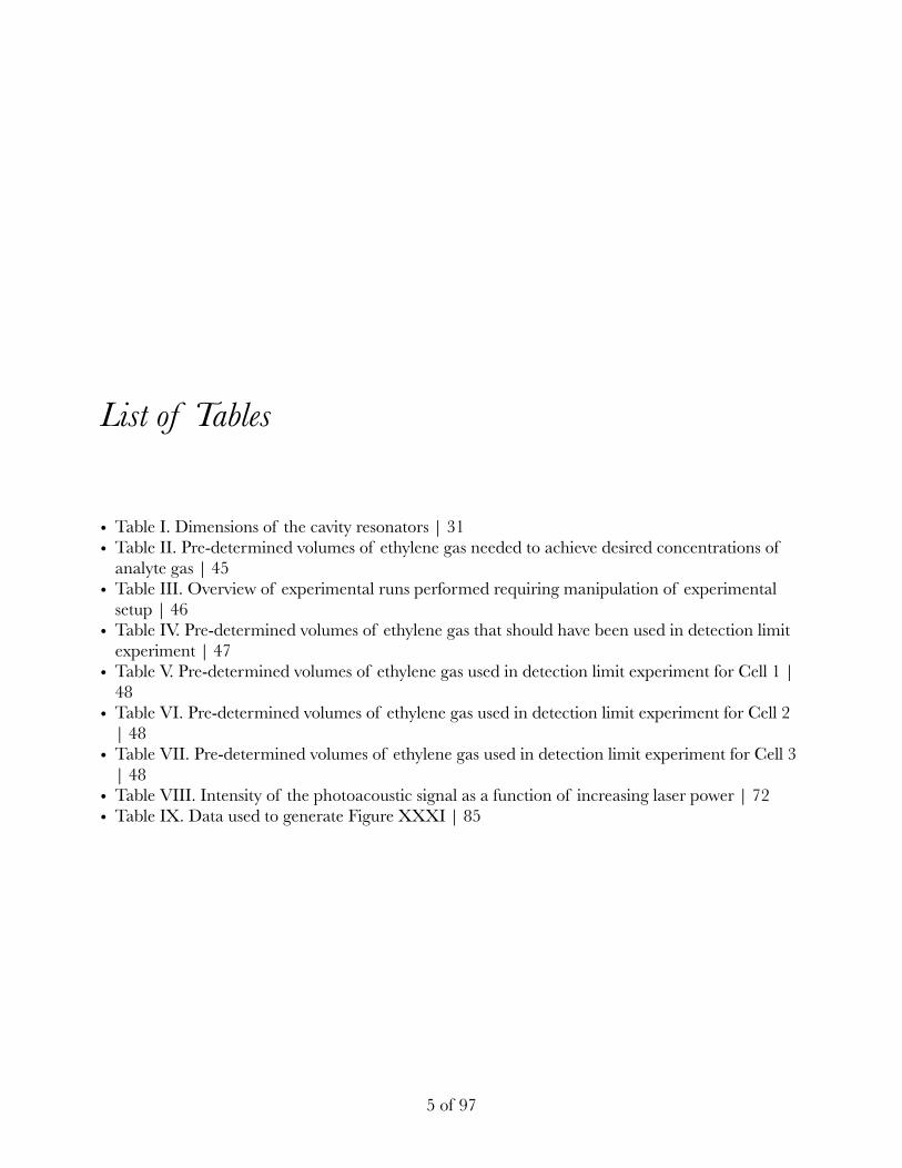
List of Tables

• Table I. Dimensions of the cavity resonators | 31 • Table II. Pre-determined volumes of ethylene gas needed to achieve desired concentrations of

analyte gas | 45 • Table III. Overview of experimental runs performed requiring manipulation of experimental

setup | 46 • Table IV. Pre-determined volumes of ethylene gas that should have been used in detection limit

experiment | 47 • Table V. Pre-determined volumes of ethylene gas used in detection limit experiment for Cell 1 |

48 • Table VI. Pre-determined volumes of ethylene gas used in detection limit experiment for Cell 2

| 48 • Table VII. Pre-determined volumes of ethylene gas used in detection limit experiment for Cell 3

| 48 • Table VIII. Intensity of the photoacoustic signal as a function of increasing laser power | 72 • Table IX. Data used to generate Figure XXXI | 85

! of !5 97

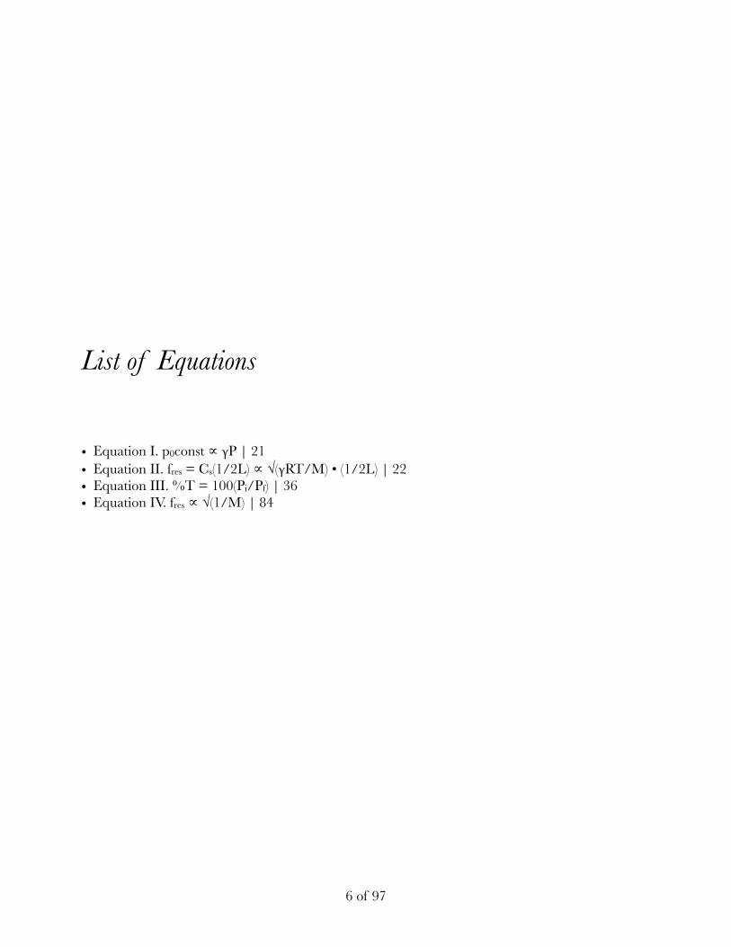
List of Equations

• Equation I. p0const ∝ γP | 21 • Equation II. fres = Cs(1/2L) ∝ √(γRT/M) • (1/2L) | 22 • Equation III. %T = 100(Pi/Pf) | 36 • Equation IV. fres ∝ √(1/M) | 84

! of !6 97

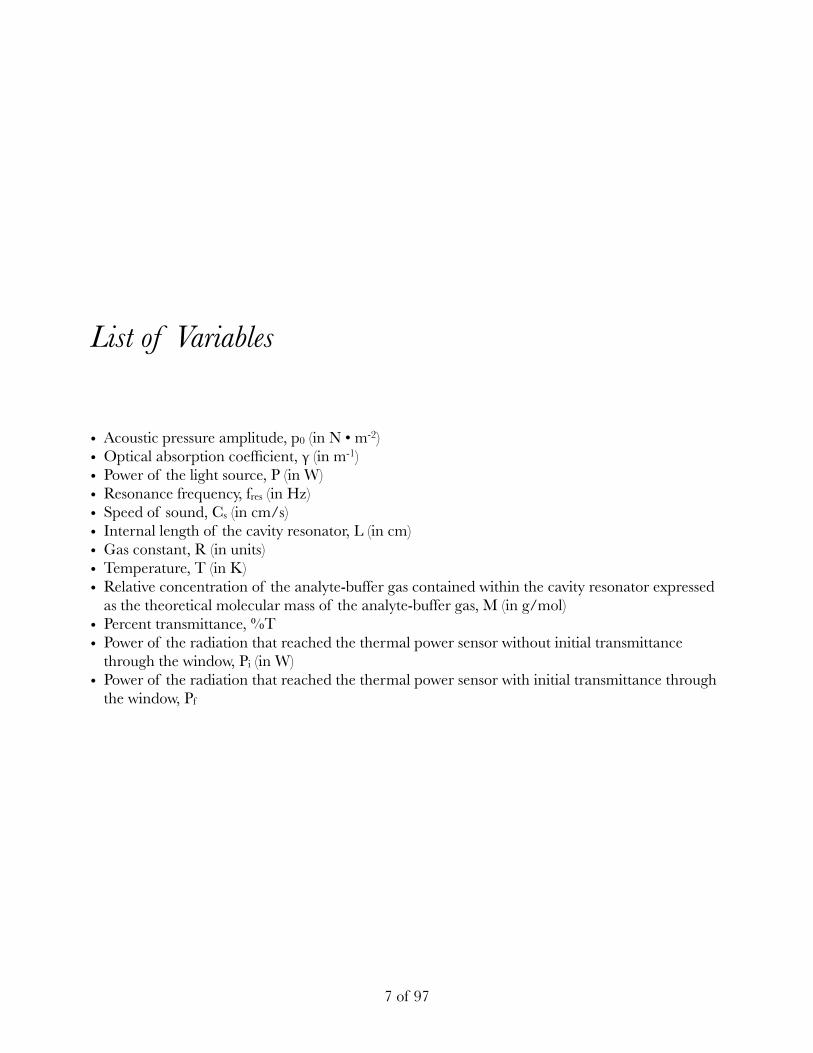
List of Variables

• Acoustic pressure amplitude, p0 (in N • m-2) • Optical absorption coefficient, γ (in m-1) • Power of the light source, P (in W) • Resonance frequency, fres (in Hz) • Speed of sound, Cs (in cm/s) • Internal length of the cavity resonator, L (in cm) • Gas constant, R (in units) • Temperature, T (in K) • Relative concentration of the analyte-buffer gas contained within the cavity resonator expressed

as the theoretical molecular mass of the analyte-buffer gas, M (in g/mol) • Percent transmittance, %T • Power of the radiation that reached the thermal power sensor without initial transmittance

through the window, Pi (in W) • Power of the radiation that reached the thermal power sensor with initial transmittance through

the window, Pf

! of !7 97

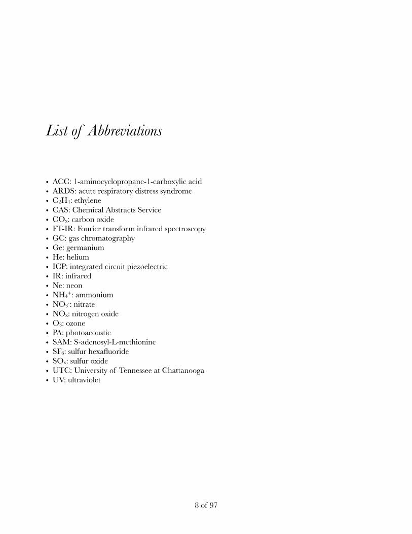
List of Abbreviations

• ACC: 1-aminocyclopropane-1-carboxylic acid • ARDS: acute respiratory distress syndrome • C2H4: ethylene • CAS: Chemical Abstracts Service • COx: carbon oxide • FT-IR: Fourier transform infrared spectroscopy • GC: gas chromatography • Ge: germanium • He: helium • ICP: integrated circuit piezoelectric • IR: infrared • Ne: neon • NH4+: ammonium • NO3-: nitrate • NOx: nitrogen oxide • O3: ozone • PA: photoacoustic • SAM: S-adenosyl-L-methionine • SF6: sulfur hexafluoride • SOx: sulfur oxide • UTC: University of Tennessee at Chattanooga • UV: ultraviolet

! of !8 97

Abstract

A Study of the Photoacoustic Effect in Ethylene Gas

By: Jay Nguyen

Ethylene, C2H4, is a plant hormone produced and released naturally by plants and soil

microorganisms. This colorless, flammable gas has a slightly sweet odor usually only recognized by

those who have handled ethylene before. In situ analyses of this gas and many other potentially

harmful gases outside of the laboratory are often difficult to perform due to the lack of a portable

yet reliable unit capable of precisely and accurately detecting and measuring the concentrations of

these gases at trace gas concentrations of a few parts per billion. In this research project,

photoacoustic spectroscopy was used to detect and measure the concentration of ethylene.

Multiple aspects of the experimental setup were independently manipulated to determine each of

their effects on the photoacoustic behavior exhibited. The data obtained in this research project

was used to help formulate a discussion about what experimental conditions were most ideal for

detection and measurement of ethylene using photoacoustic spectroscopy. It was determined that

this technique was most reliable when the internal radius of the cavity resonator was small, the

power of the light source was high, the concentration of ethylene gas was high, and the rotational

frequency of the mechanical chopper was low. These experimental conditions should be

considered by manufacturers when devising highly-sensitive, low-cost portable systems for the

detection and measurement of ethylene gas both inside and outside the laboratory.

! of !9 97

Chapter 1: Introduction

Table of Contents

• 1.1: Importance of trace gas detection

• 1.2: Importance of trace ethylene detection

• 1.3: Overview of current trace gas detection techniques

• 1.4: Introduction to photoacoustic spectroscopy as an effective trace gas detection technique

• 1.5: Statement of intent

1.1: Importance of trace gas detection

The idea that unregulated levels of gases can pose adverse health effects on humans and

other living organisms is well supported. There exist numerous arguments supporting the need for

advanced trace gas detection and analysis techniques. Such claims are often driven by those

heavily invested in environmental, microbiological, and/or medical research (1, 2).

Among the many applications of environmental research include targeted studies involving

the chemical makeup of the atmosphere, particularly within the troposphere. Such atmospheric

chemicals include sulfur oxides, SOx, nitrogen oxides, NOx, carbon oxides, COx, and various other

! of !10 97

pollutants and greenhouse gases (1). Perhaps one of the most well-known but not necessarily well-

understood chemicals is ozone, O3. Ozone is commonly used to sterilize medical tools, to treat

water, and to help preserve food. The creation of a hole around the stratosphere and troposphere

and the subsequent increase in solar ultraviolet (UV) radiation into the Earth’s atmosphere due to

the partial destruction of the ozone layer has generated global concern among scientists and

nonscientists over the years. At low concentrations, ozone exposure has been linked to respiratory

problems, skin rashes, and irritation to the eyes. Therefore, the ability to reliably detect and

measure the concentration of chemicals in the environment at any level is of paramount

importance (3). Within the field of microbiology, trace gas detection and analysis techniques such

gas chromatography together with flame ionization detection and gas chromatography together

with photon ionization detection are utilized to better understand the occurrence of nitrogen

fixation in nature. Many biological systems cannot metabolize molecular nitrogen; they must first

convert, or fix, diatomic nitrogen into some other usable form such as ammonium ion, NH4+, or

nitrate ion, NO3-. The nitrogen fixation process can be better understood by observing the

production of either of these two nitrogenous compounds. A medical application of trace gas

detection involves the physical and chemical analyses of exhaled air to help diagnosis some

common conditions. Gases produced via the body’s natural metabolic processes can accumulate

within the lungs before being exhaled. Exhaled air with a sweet odor can indicate uncontrolled

diabetes, a fishy odor can indicate advanced liver disease, and an urine-like odor can indicate

kidney failure (2).

There exist numerous other practical applications supporting the need for advanced trace

gas detection techniques. Another practical application of trace gas detection involves the

! of !11 97

combined use of physical chemistry and analytical chemistry to detect and measure the

concentration of the chemical ethylene.

1.2: Importance of trace ethylene detection

Ethylene, C2H4, is a phytohormone, or plant hormone, produced and released naturally by

plants and soil microorganisms (4, 5). This plant hormone is actively involved in almost all stages

of plant development. Seed growth and germination, leaf growth, and leaf and fruit abscission are

among the many plant processes regulated by ethylene (6). For climacteric fruits, or fruits that

continue to ripen after being harvested, the presence of ethylene further encourages ripening. For

non-climacteric fruits, or fruits that do not continue to ripen after being harvested, the presence of

ethylene further encourages deterioration or senescence. The extent to which each of these

processes occur depends generally upon both the concentration of ethylene present and the

duration of ethylene exposure (7). The term “concentration” refers to the partial pressure of a

particular gas in a gas solution.

Plants are often categorized according to the amount of ethylene they naturally release. For

example, “very low” ethylene releasing plants release less than 0.1 microliters ethylene per

kilogram per hour at 20ºC, while “very high” ethylene releasing plants release greater than 100

microliters (or 1 milliliter) ethylene per kilogram per hour at 20ºC. The rate at which a plant

develops will be faster in a confined and/or poorly-ventilated space than in an unconfined and/or

well-ventilated space. In a confined space, the concentration of ethylene present will likely increase

before it can decrease. On the other hand, in an unconfined space, the concentration of ethylene

present will likely decrease before it can increase (7). Ethylene’s odor is typically only recognized by

those who have handled ethylene before. The most common route of ethylene entry in humans

! of !12 97

occurs via inhalation (5). Adverse health effects occur when the amount of oxygen in the air

displaced by ethylene approaches 20% by volume or more (4, 8). Furthermore, ethylene gas is

flammable at concentrations between 27,000 - 360,000 parts per million (ppm) or 2.7 - 36.0% by

volume in air; therefore, advanced techniques that enable reliable detection and accurate

measurement of ethylene gas are of great importance from a medical point-of-view, in agriculture,

or in any other industrial or laboratory setting where ethylene is handled (8).

1.3: Overview of current trace gas detection techniques

Traditional trace gas analysis techniques include, but are not limited to, Fourier transform

infrared spectroscopy (FT-IR), non-dispersive IR spectroscopy, and various gas chromatography-

based techniques (9). Very few techniques are both portable enough for use outside of the

laboratory setting and precise and accurate enough for reliable detection and measurement at

preferably low concentrations (2). In a recent study, three techniques considered for use in fruit

supply chains were employed to detect and measure the concentration of various samples of the

chemical ethylene. These three techniques, which included non-dispersive IR spectroscopy,

miniaturized gas chromatography, and electrochemical measurement, each presented their own

unique advantages and disadvantages rendering neither one optimal for use. Specifically, among

the three techniques considered, advantages of non-dispersive IR spectroscopy, miniaturized gas

chromatography, and electrochemical measurement included relatively fast measurement, good

accuracy, and high resolution, respectively. On the other hand, disadvantages of non-dispersive IR

spectroscopy, miniaturized gas chromatography, and electrochemical measurement included

relatively poor sensitivity, slow measurement, and high cost, respectively (4). Therefore, there exists

a need for some other more advantageous trace ethylene detection technique.

! of !13 97

1.4: Introduction to photoacoustic spectroscopy as an effective trace gas detection

technique

Photoacoustic (PA) spectroscopy refers to the application of the PA effect for spectroscopic

purposes (9). This phenomenon, first discovered in 1880, grew in popularity nearly half a century

after its initial discovery upon discovery of the microphone and laser (10). The PA effect can be

summarized into the following three major steps: the localized release of heat from a sample of gas

within a cavity resonator, the generation of acoustic waves due to this release of heat, and the

detection and measurement of the acoustic signal produced (9, 10). How the PA effect occurs is

explained in further detail in Chapter 2: Background.

This technique is especially useful for detecting and measuring the concentration of

strongly absorbing gases, or gases with high absorption coefficients. Recent research on the PA

effect of sulfur hexafluoride, SF6, revealed that standing waves within a cavity resonator had

different amplitudes at different microphone positions (11). Furthermore, it was determined that

the modulation frequency at which PA resonance occurs for sulfur hexafluoride varied depending

upon the internal length of the cavity resonator, the temperature within the cavity resonator, and

the concentration of the gas sample contained within the cavity resonator expressed as a function

of the molecular mass of the gas solution (12).

1.5: Statement of intent

Compared with more traditional spectroscopic and trace gas analysis techniques,

knowledge of the use of PA spectroscopy as an effective technique for chemical analysis appears

far less widespread among chemists and bio-environmental scientists. There is even less

! of !14 97

documentation addressing the PA behavior of the plant hormone ethylene. This project seeks to

contribute to the current understanding of the PA effect of ethylene gas by identifying how various

facets of this technique can be manipulated to enhance its usability.

In this research project, various aspects of the experimental setup in this research project

will be independently manipulated to determine each of their effects on the PA signal produced by

ethylene. These aspects include the internal diameter of the cavity resonator, power of the light

source, concentration of analyte gas contained within the cavity resonator, and rotational

frequency of the mechanical chopper. Furthermore, the dimensions of the cavity resonator will be

manipulated to determine whether the detection limit of ethylene is affected as a result.

Theory found in physical and online references paired with data obtained in the UTC

Department of Chemistry and Physics research laboratory will be used to help formulate a

discussion about the PA effect of ethylene gas. By better understanding the experimental

conditions that best enable precise and accurate measurements of ethylene, manufacturers can

better create highly-sensitive, low-cost, portable systems that can still deliver reliable continuous

measurements both inside and outside of the traditional laboratory setting.

! of !15 97

Chapter 2: Background

Table of Contents

• 2.1: History of photoacoustic effect

• 2.2: Breakdown of photoacoustic spectroscopy

• 2.3: About ethylene

2.1: History of photoacoustic effect

The PA effect was discovered by Alexander Graham Bell in 1880 when he noticed that thin

discs exposed to a rapidly interrupted beam of light produced sound. In a later experiment, Bell

placed absorbing substances inside a spectroscope at the focal point and observed sound in all parts

of the sun’s electromagnetic spectrum using a hearing tube (2). Through his experiments, Bell

proposed that gas, liquid, and solid materials exposed to modulated radiation produced acoustic

waves that could be both detected and measured (11). Due to the lack of a proper light source,

microphone, and electronics, the PA effect was left unstudied for nearly half a century (10). Few

advancements in the study of the PA effect were observed during this time until the discovery of

the microphone in 1938 and the laser in the 1960s (13, 2). The discovery of the laser brought

! of !16 97

about improved beam quality, spectral purity, and power (in comparison to other conventional light

sources) (10). Scholars Kerr and Atwood were among the first to combine laser technology with the

PA effect to obtain absorption spectra of small gas molecules in the late 1960s (2). Scholars

Kreuzer and Patel both incorporated this phenomenon into their studies of gases in the early

1970s (14). Using an IR Ne-He laser (3 μm), Kreuzer was able to detect and measure

concentrations of methane gas in nitrogen gas to 10 parts per billion (ppb). Patel was able to detect

and measure concentrations of nitrogen monoxide and water at high altitudes using a balloon-

borne spin-flip Ramen laser. Other noteworthy scholars that contributed to today’s understanding

of the PA effect include scholars Röntgenx, Tyndall, Preece, Viegerov, and Luft. Recent

advancements in the PA research include applications of trace gas detection for environmental,

biological, and medical purposes (2).

2.2: Breakdown of photoacoustic spectroscopy

Photoacoustic spectroscopy refers to the application of the PA effect for spectroscopic

purposes (9). The mathematical theory behind the PA effect is complicated, yet the effect, itself,

can be summarized into the following three major steps: the localized release of heat from a

sample of gas due to the excitation and subsequent de-excitation of the sample’s internal energy

levels, the generation of acoustic waves due to this heat release, and the detection and

measurement of the acoustic signal produced within a cavity resonator using a microphone (9, 10).

Electromagnetic radiation in the form of photons, or massless particles containing energy,

is emitted from a continuous-wave light source and directed through the window of a cylindrical

cavity resonator (14). This radiation must have a wavelength that falls within the range of

wavelengths permitted by the window; otherwise, the radiation will not be able to enter the cavity

! of !17 97

resonator and the PA effect will not be observed (12). Prior to entering the cavity resonator, the

radiation emitted from the light source is modulated using a mechanical chopper together with a

frequency modulator. The frequency at which this mechanical chopper rotates can be set and

adjusted using the frequency modulator (10). Using the frequency modulator, the rotational

frequency of the mechanical chopper can range anywhere from single value to several thousand

hertz (Hz) (15). As the radiation emitted from the continuous-wave light source passes through the

rotating mechanical chopper, the radiation is modulated or intermittently broken up at a frequency

proportional to the rotational frequency of the mechanical chopper (10). Upon entering the cavity

resonator, photons emitted from the light source can strike the analyte gas molecules contained

within. The absorption of the incident photons by the analyte gas molecules causes the internal

energy levels within the sample to become excited to a higher quantum state. The de-excitation of

these internal energy levels within the sample can occur via radiative or non-radiative processes.

The excitation and de-excitation of the internal energy levels occur at a frequency influenced by

but not directly proportional to the rotational frequency of the mechanical chopper (16). The

frequency at which the internal energy levels become excited and de-excited cannot be directly

proportional to the rotational frequency of the mechanical chopper due to the fact that the

frequency at which the excitation and de-excitation takes place is several orders of magnitude

greater than any rotational frequency that a mechanical chopper can achieve. Radiative processes

include spontaneous or stimulated emission, while non-radiative processes include intermolecular

collisions (16). Radiative relaxation processes will not be discussed in this thesis. Non-radiative

relaxation to the ground state via intermolecular colliding results in the transformation of energy

lost into translational kinetic energy. This loss of energy presents in the form of heat. Thermal

changes in an isochoric system in which the volume remains constant results in pressure change

! of !18 97

(15). The intermittent excitation and de-excitation of the internal energy levels causes fluctuations

in pressure within the cavity resonator (17). These pressure fluctuations are the direct result of

force (in the form of mechanical waves) being generated as the analyte gas molecules seek to

minimize the localized stress caused by the subsequent excitation and de-excitation of their

internal energy levels. (13). These fluctuations in pressure present in the form of measurable

infrasonic, audible, or ultrasonic waves that can be detected and transduced, or converted from

one form into another, using a microphone. At any point in time, these mechanical waves traverse

along longitudinal eigenmodes, along radial eigenmodes, or both. At modulation frequencies

below 1 Hz, these pressure fluctuations manifest in the form of infrasonic waves; at modulation

frequencies between 16 Hz and 16 kHz, these pressure fluctuations manifest in the form of audible

waves, and at modulation frequencies greater than 16 kHz, these pressure fluctuations manifest in

the form of ultrasonic waves (13).

In PA spectroscopic experiments, microphones are used as a type of piezoelectric

transducer. These types of transducers are capable of converting mechanical fluctuations or

changes in physical quantities to electrical signals that can be observed using the proper electronics.

As the microphone picks up acoustic waves generated within the cavity resonator, it converts these

mechanical fluctuations into electrical signals that manifest as a visible waveform that can be seen

using an oscilloscope and heard using a speaker (11). This waveform has an amplitude

proportional in magnitude to the number of incident photons absorbed by the analyte gas which

may depend upon the number of analyte gas molecules contained within the cavity resonator—

expressed as a particular concentration of analyte gas—when the number of incident photons

entering the cavity resonator is kept constant, or it may depend upon the number of incident

photons entering the cavity resonator—expressed as the power of the light source emitting the

! of !19 97

photons—when the number of analyte gas molecules contained within the cavity resonator is kept

constant. As previously mentioned, the word “concentration” refers to the partial pressure of a

particular gas in a gaseous solution held at some arbitrary total pressure. Throughout this research

project, the word “concentration” was used to describe the amount of analyte gas, or the partial

pressure of the analyte gas, contained within a cavity resonator. In an isochoric system, the sum of

the partial pressures of the analyte gas and the buffer gas equals the total pressure within the cavity

resonator. For example, an analyte-buffer gas solution with an analyte gas concentration of 25% by

volume will have enough analyte gas to contribute 25% towards the total pressure within the cavity

resonator and enough buffer gas to contribute the remaining 75% towards the total pressure. In

this case, if the total pressure within the cavity resonator is 1.0 atmosphere (atm), the partial

pressure of the analyte gas will be 0.25 atm, and the partial pressure of the buffer gas will be 0.75

atm.

The typical waveforms of a PA signal (shown as an orange/yellow waveform) and the

typical waveform of a reference signal (shown as a blue waveform) can both be found in Figure I.

! of !20 97

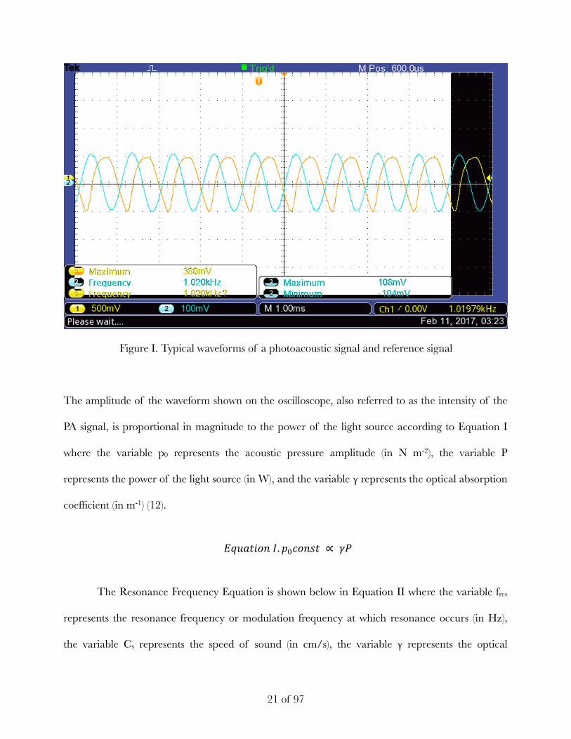
Figure I. Typical waveforms of a photoacoustic signal and reference signal

The amplitude of the waveform shown on the oscilloscope, also referred to as the intensity of the

PA signal, is proportional in magnitude to the power of the light source according to Equation I

where the variable p0 represents the acoustic pressure amplitude (in N m-2), the variable P

represents the power of the light source (in W), and the variable γ represents the optical absorption

coefficient (in m-1) (12).

The Resonance Frequency Equation is shown below in Equation II where the variable fres

represents the resonance frequency or modulation frequency at which resonance occurs (in Hz),

the variable Cs represents the speed of sound (in cm/s), the variable γ represents the optical

! of !21 97

Cell # Internal Length (cm) Internal Radius (cm) Internal Volume (mL)

1 45.0 0.953 95.27 2 44.0 1.91 341.77 3 45.0 2.54 649.03

!"#$%&'(*. ,-.'(/% ∝ 12

!"#$%&'(**. 3456 = 8612; ∝ 1<=

> × 12;

!"#$%&'(***. 3456 = 1>

Cell # Volume of Ethylene Gas Needed to Achieve Desired Concentrations of Analyte Gas (mL) 5% 10% 25% 50% 100%

1 4.764 9.527 23.82 47.64 95.27 2 17.089 34.177 85.443 170.89 341.77 3 32.452 64.903 162.26 324.52 649.03

Run

Cell [Internal Radius of

Cavity Resonator

(cm)]

Concentrations of Analyte Gas Contained Within Cavity

Resonator (%) [Volume of Analyte Gas Needed to

Achieve Desired Concentrations (mL)]

Rotational Frequency of Mechanical

Chopper (Hz)

Power of Light Source (%) [Exact Power of

Light Source (mW)]

Windows

1 (0.953) 2 (1.91) 3 (2.54)

4 (unknown)

5 10 25 50

100

200 - 4000 250 100 (291.0)

(1st, 2nd) C: coated

UC: uncoated

A 1 (0.953) 5 (4.764) 200 - 4000 100 (291.0) (C, C) B 1 (0.953) 10 (9.527) 200 - 4000 100 (291.0) (C, C) C 1 (0.953) 25 (23.82) 200 - 4000 100 (291.0) (C, C) D 1 (0.953) 50 (47.64) 200 - 4000 100 (291.0) (C, C) E 1 (0.953) 100 (95.27) 200 - 4000 100 (291.0) (C, C) F 2 (1.91) 5 (17.089) 200 - 4000 100 (291.0) (C, C) G 2 (1.91) 10 (34.177) 200 - 4000 100 (291.0) (C, C) H 2 (1.91) 25 (85.443) 200 - 4000 100 (291.0) (C, C) I 2 (1.91) 50 (170.89) 200 - 4000 100 (291.0) (C, C) J 2 (1.91) 100 (341.77) 200 - 4000 100 (291.0) (C, C) K 3 (2.54) 5 (32.452) 200 - 4000 100 (291.0) (C, C) L 3 (2.54) 10 (64.903) 200 - 4000 100 (291.0) (C, C) M 3 (2.54) 25 (162.26) 200 - 4000 100 (291.0) (C, C) N 3 (2.54) 50 (324.52) 200 - 4000 100 (291.0) (C, C)

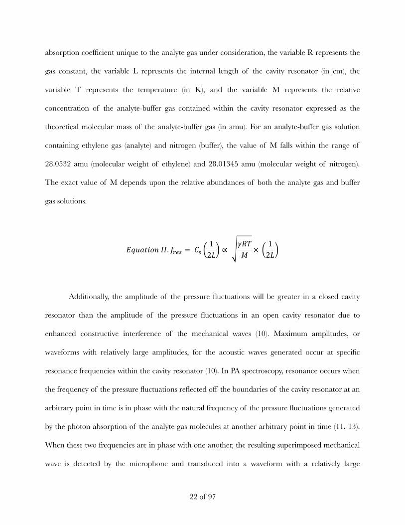
absorption coefficient unique to the analyte gas under consideration, the variable R represents the

gas constant, the variable L represents the internal length of the cavity resonator (in cm), the

variable T represents the temperature (in K), and the variable M represents the relative

concentration of the analyte-buffer gas contained within the cavity resonator expressed as the

theoretical molecular mass of the analyte-buffer gas (in amu). For an analyte-buffer gas solution

containing ethylene gas (analyte) and nitrogen (buffer), the value of M falls within the range of

28.0532 amu (molecular weight of ethylene) and 28.01345 amu (molecular weight of nitrogen).

The exact value of M depends upon the relative abundances of both the analyte gas and buffer

gas solutions.

Additionally, the amplitude of the pressure fluctuations will be greater in a closed cavity

resonator than the amplitude of the pressure fluctuations in an open cavity resonator due to

enhanced constructive interference of the mechanical waves (10). Maximum amplitudes, or

waveforms with relatively large amplitudes, for the acoustic waves generated occur at specific

resonance frequencies within the cavity resonator (10). In PA spectroscopy, resonance occurs when

the frequency of the pressure fluctuations reflected off the boundaries of the cavity resonator at an

arbitrary point in time is in phase with the natural frequency of the pressure fluctuations generated

by the photon absorption of the analyte gas molecules at another arbitrary point in time (11, 13).

When these two frequencies are in phase with one another, the resulting superimposed mechanical

wave is detected by the microphone and transduced into a waveform with a relatively large

! of !22 97

Cell # Internal Length (cm) Internal Radius (cm) Internal Volume (mL)

1 45.0 0.953 95.27 2 44.0 1.91 341.77 3 45.0 2.54 649.03

!"#$%&'(*. ,-.'(/% ∝ 12

!"#$%&'(**. 3456 = 8612; ∝ 1<=

> × 12;

!"#$%&'(***. 3456 = 1>

Cell # Volume of Ethylene Gas Needed to Achieve Desired Concentrations of Analyte Gas (mL) 5% 10% 25% 50% 100%

1 4.764 9.527 23.82 47.64 95.27 2 17.089 34.177 85.443 170.89 341.77 3 32.452 64.903 162.26 324.52 649.03

Run

Cell [Internal Radius of

Cavity Resonator

(cm)]

Concentrations of Analyte Gas Contained Within Cavity

Resonator (%) [Volume of Analyte Gas Needed to

Achieve Desired Concentrations (mL)]

Rotational Frequency of Mechanical

Chopper (Hz)

Power of Light Source (%) [Exact Power of

Light Source (mW)]

Windows

1 (0.953) 2 (1.91) 3 (2.54)

4 (unknown)

5 10 25 50

100

200 - 4000 250 100 (291.0)

(1st, 2nd) C: coated

UC: uncoated

A 1 (0.953) 5 (4.764) 200 - 4000 100 (291.0) (C, C) B 1 (0.953) 10 (9.527) 200 - 4000 100 (291.0) (C, C) C 1 (0.953) 25 (23.82) 200 - 4000 100 (291.0) (C, C) D 1 (0.953) 50 (47.64) 200 - 4000 100 (291.0) (C, C) E 1 (0.953) 100 (95.27) 200 - 4000 100 (291.0) (C, C) F 2 (1.91) 5 (17.089) 200 - 4000 100 (291.0) (C, C) G 2 (1.91) 10 (34.177) 200 - 4000 100 (291.0) (C, C) H 2 (1.91) 25 (85.443) 200 - 4000 100 (291.0) (C, C) I 2 (1.91) 50 (170.89) 200 - 4000 100 (291.0) (C, C) J 2 (1.91) 100 (341.77) 200 - 4000 100 (291.0) (C, C) K 3 (2.54) 5 (32.452) 200 - 4000 100 (291.0) (C, C) L 3 (2.54) 10 (64.903) 200 - 4000 100 (291.0) (C, C) M 3 (2.54) 25 (162.26) 200 - 4000 100 (291.0) (C, C) N 3 (2.54) 50 (324.52) 200 - 4000 100 (291.0) (C, C)

amplitude. For an isochoric system, the frequency and magnitude of the pressure fluctuations

generated by the analyte gas molecules will depend upon the rotational frequency and duty cycle,

respectively, of the mechanical chopper.

Again, a continuous-wave light source and a mechanical chopper together with a frequency

modulator are typically employed in PA spectroscopy; however, the radiation may also be pulsed

(versus modulated) by the light source, itself, prior to entering the cavity resonator. At low

modulation frequencies and pulsation frequencies, the excited internal energy levels of the analyte

gas molecules will have more time to relax back down to the ground state before being re-excited

upon reabsorption of photons from the light source. The resulting pressure fluctuations will,

therefore, be well-separated both in time and in space. As the modulation frequency and pulsation

frequency increases, the time in between each consecutive excitation and de-excitation decreases,

resulting in pressure fluctuations that are more difficult to distinguish among one another (17). This

phenomenon can be attributed to the fact that heat pulses last somewhat longer than the light

pulses; in other words, the amount of time it takes for the internal energy levels to relax back down

to the ground state is typically longer than the amount of time it takes for the internal energy levels

to become excited in the first place (10). With modulated radiation, the gas molecules contained

within the cavity resonator spend as much time exposed to the photons from the light source as

they do shielded from the photons, resulting in a 50% duty cycle. With pulsed radiation, the gas

molecules spend more time shielded from the photons than they do exposed, resulting in a lower

duty cycle (17). At very low duty cycles, the resulting pressure fluctuations will also be well-

separated in time and in space but small in magnitude, while at very high duty cycles, the resulting

pressure fluctuations will be poorly-separated. Analyte gas molecules exposed to radiation with a

! of !23 97

50% duty cycle will result in pressure fluctuations that are both well-separated and large in

magnitude (10).

An analysis of the PA effect of any sample reveals information about the transient flow of

heat to and from that sample. It can be argued that application of the PA technique is as much a

form of calorimetry as it is a form of optical absorption spectroscopy (9). A gas solution with a

high concentration of analyte gas molecules will absorb more photons, release more heat, and thus

generate larger pressure fluctuations than a gas solution with a relatively lower concentration of

analyte gas molecules, which will absorb less photons, release less heat, and thus generate smaller

pressure fluctuations. PA spectroscopy can, therefore, be used to measure the concentration of any

analyte gas molecule contained within a gas solution.

2.3: About ethylene

Dimitry Nikolayevich Neljubov, a researcher at the Botanical Institute in St. Petersburg,

discovered ethylene in the 19th century when he noticed this gaseous chemical caused his pea

seedlings to grow horizontally, making it the first phytohormone ever identified. The rise of gas

chromatography technique in the late 20th century brought about increased awareness and respect

for ethylene as a self-regulator of plant growth and development (6). This phytohormone has been

known to help regulate seed germination, the adjustment of seedlings to soil conditions, color

change, degreening of citrus fruits, and the development, senescence, and abscission of leaves (6,

7). Negative effects of ethylene often include reduced storage life, increased oxidative browning,

and quickened senescence. More specific adverse effects of ethylene include the formation of

bitter-tasting chemicals in carrots, russet spotting on lettuce, and inhibited blooming of carnations

(7).

! of !24 97

Naturally, ethylene is generated by plants metabolically via the conversion of S-adenosyl-L-

methionine (SAM) into ethylene through the methionine cycle. There are two catalysis reactions

involved in this process. First, SAM is converted into the cyclic amino-acid intermediate 1-

aminocyclopropane-1-carboxylic acid (ACC) using the enzyme ACC synthase. Finally, ACC is

converted into ethylene (with cyanide as a byproduct) using the enzyme ACC oxidase (6, 7).

In addition to its natural occurrence and use as a plant hormone, ethylene, formerly used

as an anesthetic, is also used as a refrigerant and in the production of alcohol, mustard gas,

petrochemicals, polymers, and resins. This chemical is a common air contaminant found in

tobacco smoke, automative and diesel exhaust and is produced via the manufacturing of

petroleum (5).

This colorless, flammable gas has a slightly sweet odor that is generally only recognized by

those who have had experience handling ethylene before. At extremely low temperatures, ethylene

may also exist as a colorless liquid (8). Ethylene is often referred to as acetene, ethene, olefiant gas,

and bicarburretted hydrogen as well. Each molecule consists of two double-bonded carbons with

two hydrogens attached to each carbon (5). Ethylene has a molecular mass of 28.05 amu (4). The

specific weight of ethylene gas (1.1718 kg/m3 at 15ºC) is similar to that of air (1.225 kg/m3 at

15ºC), thus making it possible for ethylene gas to dissipate evenly in air. The ability of ethylene gas

to dissipate evenly in air can be both useful or harmful, depending on the setting. Free-flowing

distribution of ethylene gas into large, open, or well-ventilated spaces like stores can induce the

slow and even ripening of fruits and vegetables, while free-flowing distribution of gas in small,

closed, or poorly-ventilated spaces like ships and trucks can force fruits and vegetables to ripen too

quickly and unevenly (4). Fruits and vegetables are often categorized according to the amount of

ethylene they naturally release. Fruits and vegetables that release less than 0.1 microliters ethylene

! of !25 97

per kilogram per hour at 20ºC, including cherry, citrus, artichoke, and asparagus, are considered

“very low” ethylene releasers; between 0.1 and 1.0 microliters ethylene per kilogram per hour are

considered “low”; between 1.0 and 10.0 microliters ethylene per kilogram per hour are considered

“moderate”; between 10.0 - 100.0 microliters ethylene per kilogram per hour are considered high;

fruits and vegetable that release greater than 100.0 microliters ethylene per kilogram per hour are

considered “very high” ethylene releasers (7).

Inhalation is the most common route of ethylene entry in humans (5). Ethylene’s ability to

travel across both short and long distances may pose serious health risks to humans if the amount

of oxygen in the air displaced by the ethylene gas, a simple asphyxiant, approaches 20% by volume

or more (4, 8). Though ethylene has a relatively short half-life of 1.9 days (5), acute overexposure

to ethylene gas has been linked to numerous respiratory and non-respiratory symptoms in humans.

These symptoms include, but are not limited to, headache, ringing in the ears, dizziness,

drowsiness, unconsciousness, nausea, and vomiting (8). It is worth noting that the majority of

ethylene inhaled is exhaled before it can enter the bloodstream. Presently, there are no known

adverse health effects linked directly to chronic exposure to ethylene gas; however, chronic

exposure to oxygen-deficient environments can cause decreased alveolar partial oxygen pressure

and induce hypoxemia, which has been linked to numerous symptoms associated with the cardiac

and central nervous system (5, 8). These symptoms include, but are not limited to, central nervous

system depression, unconsciousness, and even death. In severe cases, acute respiratory distress

syndrome (ARDS) and/or other acute and potentially life-threatening lung injuries may develop.

The signs and symptoms for these conditions may not develop for at least 24 hours but usually by

72 hours. Contact exposure of liquid ethylene to human skin can result in local frostbite at the site

of contact and other forms of skin irritation, while contact exposure to the eyes can cause redness

! of !26 97

and burning. Entry of ethylene gas in humans via ingestion can lead to irritation of the

gastrointestinal tract; however, toxicologically significant levels of ethylene rarely are absorbed by

the digestive tract (5).

It is, therefore, imperative that ethylene in both its gas and liquid form be handled with

caution. Ethylene should be stored in unconfined and/or well-ventilated spaces as a precautionary

measure to prevent the build-up of ethylene gas to potentially explosive concentrations. In the

event of a cylinder leak that cannot be sealed, sources of ignition should be shut off, the area

should be evacuated, and the cylinder should be relocated to an open-air space and emptied (5).

The slightly sweet odor of ethylene can be detected by humans between concentrations of

260 - 4000 ppm, rendering odor, alone, an unreliable indicator of possible overexposure to

ethylene (5). In situ measurements of ethylene concentration outside of the laboratory are difficult

to perform due to the lack of a portable yet sensitive unit capable of accurately and repeatedly

detecting at preferred resolutions of a few ppb. Therefore, presently, measurements of ethylene

concentration are performed using stationary equipment found in laboratories or in other similar

environments (4).

! of !27 97

Chapter 3: Materials and Methodology

Table of Contents

• 3.1: Materials

• 3.2: Methodology

• 3.2.1: Part 1: Infrared spectra for ethylene and nitrogen

• 3.2.2: Part 2: Experimental runs with manipulated parameters

• 3.2.3: Part 3: Detection limit experiment

3.1: Materials

The terms “PA cell” and “PA detector” are often used interchangeably. The two terms,

however, do not refer to the same thing. The PA cell includes those components that make up the

acoustic unit. This acoustic unit includes an analyte gas, a buffer gas, a cavity resonator, a pair of

windows, and a microphone. On the other hand, the PA detector includes all components that

make up the instrument. In addition to those components that make up the acoustic unit, the PA

detector includes a light source, a gas handling system, and any electronics necessary for gas

detection (10).

! of !28 97

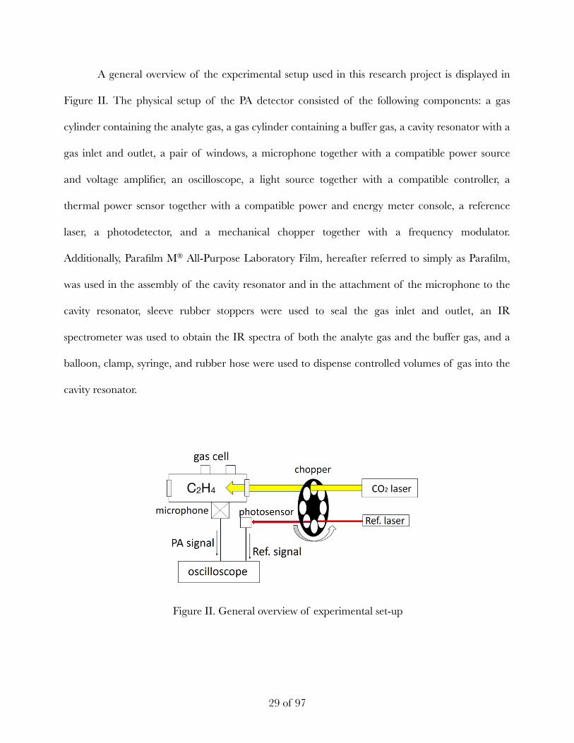
A general overview of the experimental setup used in this research project is displayed in

Figure II. The physical setup of the PA detector consisted of the following components: a gas

cylinder containing the analyte gas, a gas cylinder containing a buffer gas, a cavity resonator with a

gas inlet and outlet, a pair of windows, a microphone together with a compatible power source

and voltage amplifier, an oscilloscope, a light source together with a compatible controller, a

thermal power sensor together with a compatible power and energy meter console, a reference

laser, a photodetector, and a mechanical chopper together with a frequency modulator.

Additionally, Parafilm M® All-Purpose Laboratory Film, hereafter referred to simply as Parafilm,

was used in the assembly of the cavity resonator and in the attachment of the microphone to the

cavity resonator, sleeve rubber stoppers were used to seal the gas inlet and outlet, an IR

spectrometer was used to obtain the IR spectra of both the analyte gas and the buffer gas, and a

balloon, clamp, syringe, and rubber hose were used to dispense controlled volumes of gas into the

cavity resonator.

Figure II. General overview of experimental set-up

! of !29 97

C2H4

In this research project, pure ethylene gas was used as the analyte gas and nitrogen gas was

used as the buffer gas. Both gases were contained within gas cylinders throughout the research

period at some unknown pressure greater than 1 atm. The Chemical Abstracts Service registry

number for ethylene is 74-85-1 (8). The Chemical Abstracts Service registry number for nitrogen is

7727-37-9 (18). Nitrogen gas was selected for use as a buffer gas for two reasons: its ability to

evenly dissipate in ethylene gas and because it is a non-IR-absorbing gas. (19). Nitrogen, which

presents as diatomic nitrogen gas in its elemental form, has a molecular mass of 28.01 amu and a

specific weight of 1.153 kg/m3 at 15ºC (18). Ethylene, as previously-mentioned, has a molecular

mass of 28.05 amu and a specific weight of 1.178 kg/m3 at 15ºC (4). Nitrogen, therefore, is

capable of dissipating evenly both in ethylene gas and in air.

In this research project, three glass cavity resonators with gas inlets and outlets were used to

hold gas solutions containing both buffer gas and analyte gas. Windows were attached to both ends

of the cavity resonators using Parafilm, and sleeve rubber stoppers were inserted into both the gas

inlets and the gas outlets. Additionally, Parafilm was used to modify the geometries of the cavity

resonators and to attach the microphone to the cavity resonators. The use of windows, sleeve

rubber stoppers, and film allowed for the construction of almost entirely closed-off cavity

resonators with defined volumes. The most common cavity resonators used in PA spectroscopy are

shaped like cylinders because the symmetry of a cylindrical cavity resonator coincides best with the

laser beam’s direction of propagation (10). The three different cylindrical cavity resonators

possessed their own unique internal radii, internal lengths, and internal volumes and were

constructed using various apparatuses. Note that the various apparatuses used to construct each

cavity resonator were not specifically designed to be used in PA spectroscopy research; therefore,

the three cavity resonators used in this research project were not perfectly cylindrical—the cavity

! of !30 97

resonators were irregularly shaped. The internal radii, internal lengths, and internal volumes for

the first cavity resonator, hereafter referred to as “Cell 1,” the second cavity resonator, hereafter

referred to as “Cell 2,” and the third cavity resonator, hereafter referred to as “Cell 3,” can be

found in Table I.

The internal radius of each cavity resonator was measured at each of their widest points.

The internal length of each cavity resonator was measured from one end of the cavity resonator to

the other, excluding the additional lengths of each window. The internal volume of Cell 1 was

approximated by enclosing the cavity resonator but leaving either the gas inlet or gas outlet open,

completely filling the cavity resonator with tap water through either the gas inlet or gas outlet,

transferring the water from the cavity resonator to a graduated cylinder (or multiple graduated

cylinders if needed), and measuring the volume of water to one decimal places (no approximation

of the second decimal place). As previously-stated, the use of windows, sleeve rubber stoppers, and

Parafilm allowed for the construction of an almost entirely closed-off cavity resonator with a

defined volume. Because the cavity resonators used in this research project were irregularly shaped,

the geometry of each cavity resonator was modified as needed using Parafilm to form the desired

cylindrical shape. Measurements of the internal volume of Cell 1 were repeated twice more for a

total of three trials. The mean of these three measurements was calculated to determine the best

Table I. Dimensions of the cavity resonators

Cell # Internal Length (cm) Internal Radius (cm) Internal Volume (mL)

1 45.0 0.953 95.3

2 44.0 1.91 341.8

3 45.0 2.54 649.0

! of !31 97

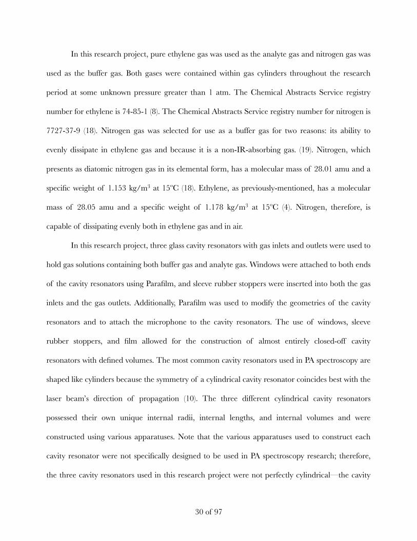
approximation for the internal volume of Cell 1. This process was repeated twice more using the

other two cavity resonators to determine the best approximation for the internal volumes of Cell 2

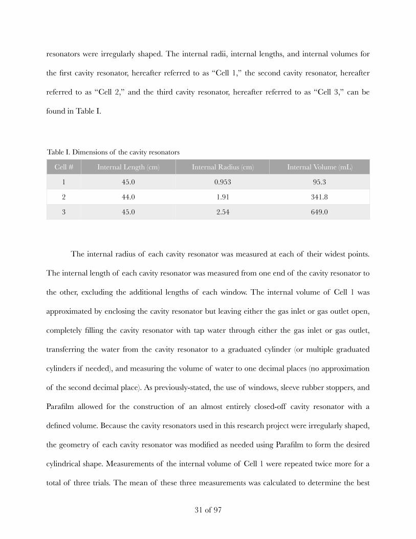
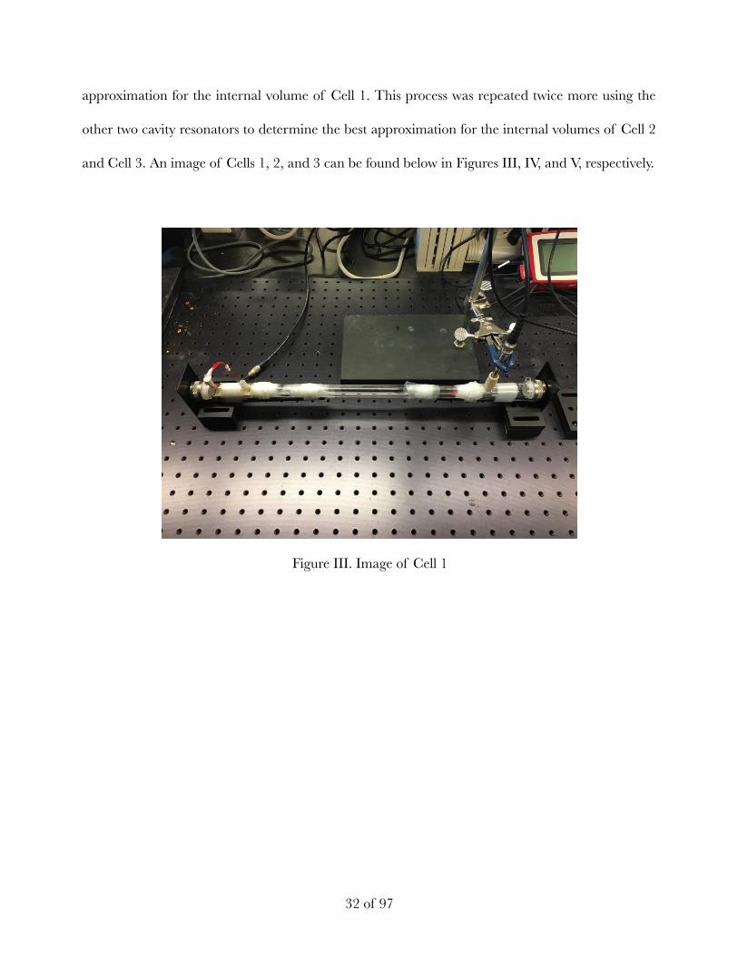
and Cell 3. An image of Cells 1, 2, and 3 can be found below in Figures III, IV, and V, respectively.

Figure III. Image of Cell 1

! of !32 97

Figure IV. Image of Cell 2

Figure V. Image of Cell 3

! of !33 97

Additionally, a fourth cavity resonator with a gas inlet and gas outlet, hereafter referred to

as “Cell 4” was used in select experimental runs when using neither Cell 1, Cell 2, nor Cell 3 were

neither necessary nor appropriate. Sleeve rubber stoppers and a set of windows were also used

with Cell 4 to allow for the construction of an almost entirely closed-off cavity resonator with a

defined volume (though the specific measurements for the internal length, internal radius, and

internal volume of this particular cavity resonator were not of significance in this research project).

In this research project, two different sets of windows were used. Windows were used to

enclose the cavity resonator and to filter the radiation that was emitted from the light source as it

entered the cavity resonator. Ethylene is IR-active at wavelengths around 10.6 μm and, therefore,

will only absorb photons with wavelengths at or around 10.6 μm. This IR-activity around the

wavelength 10.6 μm corresponds to a vibrational mode that occurs around the frequency 943 cm-1.

At this frequency, a CH2 wag will occur. It is, therefore, necessary that the windows used in this

research project also be capable of transmitting radiation at or around this wavelength. If the

radiation emitted from the light source does not have a wavelength that falls within the range of

wavelengths permitted by the window, the PA effect will not be observed. The first set of windows

used in this research project (model number, WG91050) were not coated with an antireflective

coating, while the second set of windows (model number: WG91050-G) were coated with an

antireflective coating. Both sets of windows were one inch diameter windows manufactured out of

the chemical germanium (Ge) and produced by ThorLabs, Inc. Both sets of windows allowed the

transmission of radiation between the wavelengths of 7 - 12 μm. The antireflective coating applied

to the Ge windows was designed to reduce the average reflectance of the incident radiation hitting

the coated Ge window to less than one percent when compared to the incident radiation hitting an

uncoated Ge window. The percent transmittance was approximated for both the set of uncoated

! of !34 97

Ge windows and the set of coated Ge windows to determine whether the difference between the

percent transmittance for the set of coated windows and the percent transmittance for the set of

uncoated windows was great enough to justify the additional expense required to obtain these

windows. To determine the percent transmittance for the set of uncoated windows, one uncoated

window was first attached to one end of Cell 4. The cavity resonator was placed directly in front of

the CO2 laser—this light source will be described in further detail later—so that the radiation’s

direction of propagation was perpendicular to the surface of the window. Using the thermal power

sensor together with the power and energy meter console—both of which will also be described in

further detail later—the output power was measured when the thermal power sensor was placed

between the cavity resonator and the CO2 laser and when the thermal power sensor was placed

behind the cavity resonator. These two measurements allowed us to directly compare the power of

the radiation that reached the thermal power sensor with and without transmittance through the

window. The two aforementioned measurements were obtained for the one uncoated window

when the controller—to be described in further detail later—was set to emit a radiation at 100%

of its maximum output power, 75% of its maximum output power, 50% of its maximum output

power, and 25% of its maximum output power. A simple calculation was performed to

approximate the percent of the radiation emitted from the light source that actually transmitted

through the window and reached the thermal power sensor. The previously-described process was

repeated once more to obtain a second approximation for the percent transmittance for the

uncoated window and repeated two additional times using one of the coated windows to

approximate the percent transmittance for the set of coated windows used in this research project.

The approximations for the percent transmittances of the set of uncoated windows and the set of

coated windows were determined to be 25.5% and 85.74%, respectively, using Equation III shown

! of !35 97

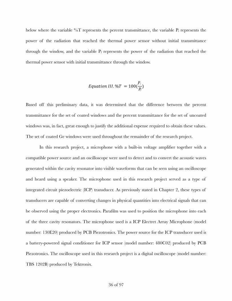
below where the variable %T represents the percent transmittance, the variable Pi represents the

power of the radiation that reached the thermal power sensor without initial transmittance

through the window, and the variable Pf represents the power of the radiation that reached the

thermal power sensor with initial transmittance through the window.

Based off this preliminary data, it was determined that the difference between the percent

transmittance for the set of coated windows and the percent transmittance for the set of uncoated

windows was, in fact, great enough to justify the additional expense required to obtain these values.

The set of coated Ge windows were used throughout the remainder of the research project.

In this research project, a microphone with a built-in voltage amplifier together with a

compatible power source and an oscilloscope were used to detect and to convert the acoustic waves

generated within the cavity resonator into visible waveforms that can be seen using an oscilloscope

and heard using a speaker. The microphone used in this research project served as a type of

integrated circuit piezoelectric (ICP) transducer. As previously stated in Chapter 2, these types of

transducers are capable of converting changes in physical quantities into electrical signals that can

be observed using the proper electronics. Parafilm was used to position the microphone into each

of the three cavity resonators. The microphone used is a ICP Electret Array Microphone (model

number: 130E20) produced by PCB Piezotronics. The power source for the ICP transducer used is

a battery-powered signal conditioner for ICP sensor (model number: 480C02) produced by PCB

Piezotronics. The oscilloscope used in this research project is a digital oscilloscope (model number:

TBS 1202B) produced by Tektronix.

! of !36 97

𝐸𝐸𝐸𝐸𝐸𝐸𝐸𝐸𝐸𝐸𝐸𝐸𝐸𝐸𝐸𝐸 𝐼𝐼𝐼𝐼𝐼𝐼. %𝑇𝑇 = 100(𝑃𝑃0𝑃𝑃 ) f

i

In this research project, a light source together with a compatible controller and a thermal

power sensor together with a compatible power and energy meter were used to excite the internal

energy levels of the analyte gas molecules and to measure the power of the radiation emitted from

the light source, respectively. Ethylene is IR-active and will only absorb photons with a wavelength

at or around 10.6 μm (7). Therefore, it is necessary that the light source together with the controller

be capable of emitting radiation at or around this same wavelength. The light source used was a

low-power continuous-wave CO2 laser (model number: L3) produced by Access Laser Company.

This particular model is capable of emitting radiation at wavelengths between 10.3 - 10.8 μm.

According to the manufacturer, the light source used in this research project is designed to have a

maximum output power of 400 mW. However, it is believed that repeat use of this particular piece

of laboratory equipment from previous research projects has forced the reduction of its maximum

output power over time. The maximum output power of the CO2 laser used in this research

project was approximated by first placing the thermal power sensor (connected to the power and

energy meter console) directly in front of the CO2 laser. The CO2 laser was turned on and set to

maximum laser power. Using the thermal power sensor together with the power and energy meter

console, the output power was measured every ten seconds for one hundred seconds. The mean of

these ten measurements was calculated to determine the best approximation for the maximum

output power. The approximation for the maximum output power for the particular light source

used in this research project was calculated to be 291.0 mW. Calculations were performed to

determine the exact power of the radiation being emitted from the light source when the CO2

laser was set to emit approximately 25%, 50%, and 75% of its maximum output power. These

powers were determined to be 72.80 mW, 145.6 mW, and 218.3 mW, respectively, by multiplying

the maximum output power for the particular light source used in this research project by 0.25,

! of !37 97

0.50, and 0.75. The thermal power sensor used was a thermal surface absorber (model number:

S310C) produced by ThorLabs, Inc. This particular model is capable of detecting radiation at

wavelengths between 0.19 - 25 μm. The power and energy meter console used in this research

project was a compact power and energy meter console (model number: PM100D) produced by

ThorLabs, Inc.

In PA spectroscopy, a reference laser and a photodetector were used to generate a noise-free

signal that could be observed on the oscilloscope. This waveform was used to help visualize

changes in the PA signal caused by the interaction of the analyte gas molecules with the photons

emitted from the previously-mentioned continuous-wave CO2 laser. The reference laser used in

this research project was a collimated laser diode module (model number: CPS182) produced by

ThorLabs, Inc. The photodetector used in this research project was a high-speed silicon

photodetector (model number: DET36A) produced by ThorLabs, Inc.

A mechanical chopper together with a frequency modulator was used to modulate both the

radiation emitted from the light source and the radiation emitted from the reference laser. As the

radiation emitted from the continuous-wave light source passed through the rotating mechanical

chopper, the radiation was intermittently broken up at a rate proportional to the rotational

frequency of the mechanical chopper. The mechanical chopper used in this research project was a

100-slot blade (model number: MC1F100) produced by ThorLabs, Inc. The frequency modulator

used in this research project was an optical chopper system (model number: MC2000B) produced

by ThorLabs, Inc. Together, the particular mechanical chopper and frequency modulator used in

this research project were capable of modulating the radiation at frequencies between 200 Hz and

10,000 Hz.

! of !38 97

Finally, an IR spectrometer was used to verify the absorption wavelengths for both the

analyte gas and buffer gas. The IR spectrometer used in this research project was a FT-IR

spectrometer (model number: Nicolet 380) produced by Thermo Scientific.

3.2 Methodology

In this research project, the following aspects of the experimental setup were intentionally

and independently manipulated to determine each of their effects on the PA signal produced by

ethylene gas: internal radius of the cavity resonator, power of the light source, concentration of

analyte gas contained within the cavity resonator, and rotational frequency of the mechanical

chopper. As previously-mentioned, each cavity resonator used in this research project was

constructed using various apparatuses not specifically designed for use in PA spectroscopy

experiments. Thus, it should be noted that experimental runs involving direct manipulation of the

internal radius of the cavity resonator yielded data were influenced by indirect manipulation of

the geometry of the cavity resonator. The methodology used in this research project is described

below in three parts. Part one describes how IR spectroscopy was used to verify that the absorption

wavelength for the buffer gas selected for use in this research project neither included nor was

around the same wavelength as the analyte gas. The second part describes how the four

aforementioned aspects of the experimental setup were manipulated to determine each of their

effects on the PA signal of ethylene. The third and final part of this research project was

performed to determine how manipulating the dimensions of the cavity resonator affected the

detection limit of ethylene.

! of !39 97

3.2.1: Part 1: Infrared spectra for ethylene and nitrogen

In the first part of this research project, IR spectroscopy was used to verify the absorption

wavelength of the analyte gas and to verify that the presence of the buffer gas used would not

unintentionally interfere with the analyte gas’s ability to absorb photons. The theoretical

wavelength at which the analyte gas, ethylene, absorbs photons is 10.6 μm; therefore, it is necessary

that the buffer gas either not be able to absorb IR radiation at all or absorb photons at a

wavelength that neither includes nor is around 10.6 μm. As previously mentioned, nitrogen gas was

selected to serve as the buffer gas because the theoretical molecular masses and specific weights of

ethylene gas and nitrogen gas in their elemental forms were both similar and because of the

characteristic inability of nitrogen gas to absorb IR radiation.

To obtain the IR spectrum of ethylene gas, the set of coated windows were first attached to

both ends of Cell 4 and a sleeve rubber stopper was inserted into both the gas inlet and outlet.

Using EZ Omnic software, the parameters of the Nicolet 380 FT-IR spectrometer were set to the

following parameters: resolution = 1 cm-1; number of scans = 16; file handling = save

automatically; background handling = collect background after 60 seconds. The background

spectrum was obtained for the cavity resonator containing no ethylene gas.

Afterward, one of the sleeve rubber stoppers was removed from either the gas inlet or gas

outlet. The cavity resonator was completely filled with ethylene gas by connecting the gas cylinder

containing pure ethylene gas to the open gas outlet (or inlet) using a rubber hose and allowing

ethylene gas to freely flow into and throughout the cavity resonator for several seconds. A sleeve

rubber stopper was inserted back into the open gas outlet (or inlet) to enclose the cavity resonator.

Without changing the parameters of the FT-IR spectrometer, the sample spectrum was obtained

for the cavity resonator containing the ethylene gas. The absorption wavelength of any given gas

! of !40 97

does not depend on the concentration of the gas sample; in other words, the wavelength at which a

particular gas within a cavity resonator absorbs photons will remain the same regardless of how

much of that particular gas is present. Therefore, the exact concentration of the ethylene gas

contained within the cavity resonator was not of significance in this research project, though it was

assumed that any undesired residual gas was expelled upon free-flowing addition of ethylene gas

into and throughout the cavity resonator.

The previously-described methodology for obtaining the IR spectrum of ethylene gas was

repeated using nitrogen gas to obtain the IR spectrum for the buffer gas. Afterward, both spectra

were compared with one another to verify that the absorption wavelength (if applicable) for the

buffer gas selected for use in this research project neither included nor was around the same

wavelength as the analyte gas.

3.2.2: Part 2: Experimental runs with manipulated parameters

In the second part of this research project, four aspects of the experimental setup were

intentionally and independently manipulated to determine each of their effects on the PA signal of

ethylene. These aspects include the internal radius of the cavity resonator, power of the light

source, concentration of analyte gas contained within the cavity resonator, and rotational

frequency of the mechanical chopper. The data obtained for each experimental run was plotted to

create a spectrum. Afterward, all spectra were compared with one another and used to help

formulate a discussion about what experimental conditions were ideal for detecting and accurately

measuring the concentration of ethylene gas using PA spectroscopic technique.

For experimental runs involving cavity resonators with varying internal radii, the three

cavity resonators, each with their own unique internal radii, were interchanged while the power of

! of !41 97

the light source remained constant. The internal radii for Cells 1, 2, and 3 can be found in Table I.

As each of the three cavity resonators were interchanged, they were placed directly in front of the

CO2 laser and oriented so that the radiation’s direction of propagation was as aligned with the

cavity resonator’s axis of symmetry as possible. For each of the three cavity resonators, the

rotational frequency of the mechanical chopper was manually increased from 200 Hz to 4000 Hz

in order to determine the intensity of the PA signal due to the interaction of the analyte gas

molecules with the photons emitted from the light source as the concentration of the analyte gas

obtained within the cavity resonator was varied. The power of the light source remained constant

for each of these experimental runs. The data sets obtained from each experimental run were used

to create spectra of PA signal intensity (in mV) versus rotational frequency of the mechanical

chopper (in Hz).

One experimental run was performed to determine what effect manipulating the power of

the light source had on the intensity of the PA signal produced. To perform this experimental run,

Cell 1, enclosed using sleeve rubber stoppers and the set of uncoated windows, was filled

completely with ethylene gas to achieve a desired concentration of 100% analyte gas. (Note that

for this particular experimental run, the set of uncoated windows was used. Because the percent

transmittance for the set of uncoated windows was previously determined to be insufficient for use

in this research project, the set of coated windows was used for all experimental runs described

hereafter.) The rotational frequency of the mechanical chopper was arbitrarily set to 250 Hz.

Using the controller for the CO2 laser, the power of the light source was gradually increased from

minimum output power to maximum output power while the concentration of the analyte gas

contained within the cavity resonator and the internal radius of the cavity resonator remained

constant. As the power of the light source was manipulated, the resulting intensity of the PA signal

! of !42 97

produced by the ethylene gas (as shown on the oscilloscope) was recorded. The thermal power

sensor together with the compatible power and energy meter console was used to measure the

exact power of the radiation being emitted from the light source as the power of the light source

was gradually increased using the controller. After recording the intensities of the PA signal as the

output power of the light source was increased from 0% to 100% of its maximum output power,

the intensities of the PA signal were adjusted to correct for any background signal that may have

presented. The data set obtained was used to create a plot of PA signal intensity (in mV) versus

laser power (in mW). For experimental runs involving a constant power of the light source, the

CO2 laser was set to emit radiation at its maximum power using the controller. As previously

mentioned, the maximum output power for the particular light source used in this research project

was experimentally-calculated to be 291.0 mW.

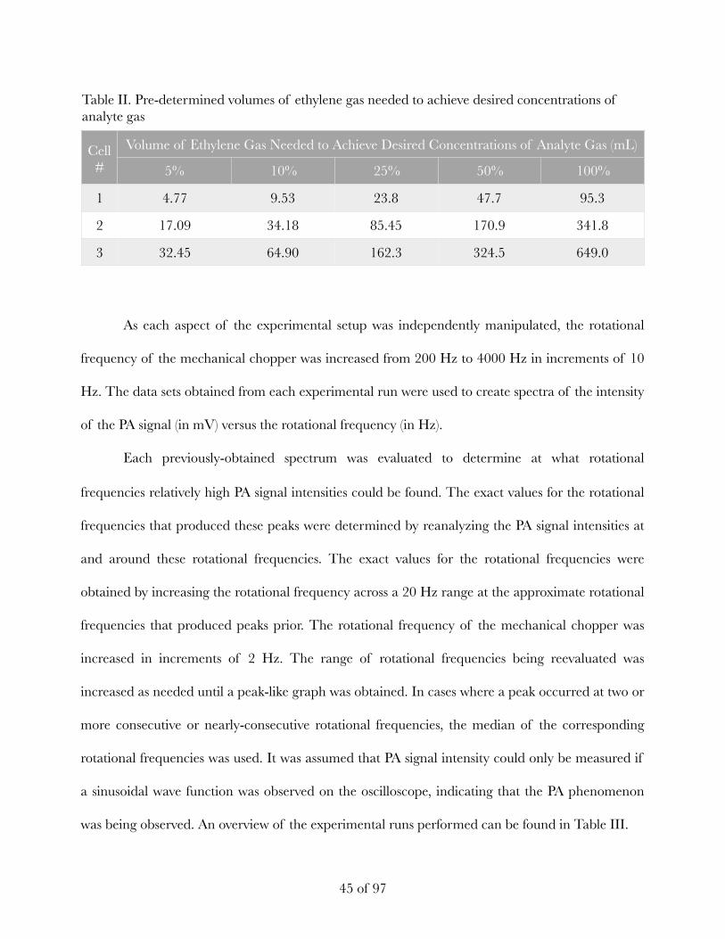
For experimental runs involving varying concentrations of analyte gas, each of the three

cavity resonators were filled with pre-determined volumes of ethylene gas to produce analyte-

buffer gas solutions with specific concentrations, represented as the percent of the internal volume

of the cavity resonator that was displaced by analyte gas or the percent of the total pressure

contributed by the analyte gas. For each of these experimental run, the power of the light source

remained constant. Similarly as before, the rotational frequency of the mechanical chopper was

manually increased from 200 Hz to 4000 Hz to determine the intensity of the PA signal under the

unique conditions established for each particular experimental run. A series of calculations were

performed to determine the volume of analyte gas that needed to be added to each cavity

resonator in order to displace 5%, 10%, 25%, 50%, and 100% of the pre-existing gas in each

cavity resonator. These volumes were determined by first approximating the internal volumes of

Cells 1, 2, and 3 and then multiplying these volumes by 0.05, 0.10, 0.25, and 0.50. Prior to each

! of !43 97

experimental run, nitrogen gas was circulated through the cavity resonator for several seconds to

rinse the cavity resonator of all residual gas that may have been left behind by other laboratory

personnel or from a previous experimental run. To rinse the cavity resonator, one of the sleeve

rubber stoppers was removed from either the gas inlet or gas outlet. The cavity resonator was

completely filled with nitrogen gas by connecting the gas cylinder containing pure nitrogen gas to

the one gas outlet (or inlet) using a rubber hose and allowing nitrogen gas to freely flow into and

throughout the cavity resonator for several seconds. To collect controlled volumes of analyte gas, a

syringe was used to draw the desired volume of gas from a sealed balloon filled with ethylene gas.

The pre-determined volumes of ethylene gas were then injected directly into the rinsed cavity

resonator through a sleeve rubber stopper. The previously-described methodology was used to

achieve desired concentrations of 5%, 10%, 25%, and 50%. It was assumed that 100%

concentration of analyte gas could be obtained by allowing ethylene gas to freely flow into and

throughout the cavity resonator. The pre-determined volumes of ethylene gas that needed to be

added to each of the three cavity resonators to achieve desired concentration of 5%, 10%, 25%,

50%, and 100% are listed in Table II. It should be noted that the particular syringes used in this

research project were capable of dispensing aliquots of ethylene gas with volumes close to but not

exactly equal to those volumes listed in Table II. The data sets obtained from each experimental

run were used to create spectra of the PA signal intensity (in mV) versus the rotational frequency

of the mechanical chopper (in Hz).

! of !44 97

As each aspect of the experimental setup was independently manipulated, the rotational

frequency of the mechanical chopper was increased from 200 Hz to 4000 Hz in increments of 10

Hz. The data sets obtained from each experimental run were used to create spectra of the intensity

of the PA signal (in mV) versus the rotational frequency (in Hz).

Each previously-obtained spectrum was evaluated to determine at what rotational

frequencies relatively high PA signal intensities could be found. The exact values for the rotational

frequencies that produced these peaks were determined by reanalyzing the PA signal intensities at

and around these rotational frequencies. The exact values for the rotational frequencies were

obtained by increasing the rotational frequency across a 20 Hz range at the approximate rotational

frequencies that produced peaks prior. The rotational frequency of the mechanical chopper was

increased in increments of 2 Hz. The range of rotational frequencies being reevaluated was

increased as needed until a peak-like graph was obtained. In cases where a peak occurred at two or

more consecutive or nearly-consecutive rotational frequencies, the median of the corresponding

rotational frequencies was used. It was assumed that PA signal intensity could only be measured if

a sinusoidal wave function was observed on the oscilloscope, indicating that the PA phenomenon

was being observed. An overview of the experimental runs performed can be found in Table III.

Table II. Pre-determined volumes of ethylene gas needed to achieve desired concentrations of analyte gas

Cell #

Volume of Ethylene Gas Needed to Achieve Desired Concentrations of Analyte Gas (mL)

5% 10% 25% 50% 100%

1 4.77 9.53 23.8 47.7 95.3

2 17.09 34.18 85.45 170.9 341.8

3 32.45 64.90 162.3 324.5 649.0

! of !45 97

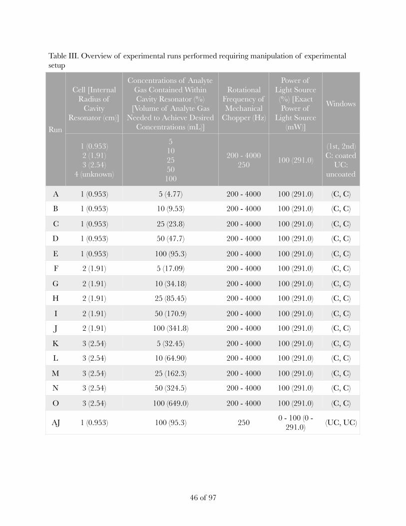
Table III. Overview of experimental runs performed requiring manipulation of experimental setup

Run

Cell [Internal Radius of

Cavity Resonator (cm)]

Concentrations of Analyte Gas Contained Within Cavity Resonator (%)

[Volume of Analyte Gas Needed to Achieve Desired

Concentrations (mL)]

Rotational Frequency of Mechanical

Chopper (Hz)

Power of Light Source (%) [Exact Power of

Light Source (mW)]

Windows

1 (0.953) 2 (1.91) 3 (2.54)

4 (unknown)

5 10 25 50 100

200 - 4000 250 100 (291.0)

(1st, 2nd) C: coated

UC: uncoated

A 1 (0.953) 5 (4.77) 200 - 4000 100 (291.0) (C, C)

B 1 (0.953) 10 (9.53) 200 - 4000 100 (291.0) (C, C)

C 1 (0.953) 25 (23.8) 200 - 4000 100 (291.0) (C, C)

D 1 (0.953) 50 (47.7) 200 - 4000 100 (291.0) (C, C)

E 1 (0.953) 100 (95.3) 200 - 4000 100 (291.0) (C, C)

F 2 (1.91) 5 (17.09) 200 - 4000 100 (291.0) (C, C)

G 2 (1.91) 10 (34.18) 200 - 4000 100 (291.0) (C, C)

H 2 (1.91) 25 (85.45) 200 - 4000 100 (291.0) (C, C)

I 2 (1.91) 50 (170.9) 200 - 4000 100 (291.0) (C, C)

J 2 (1.91) 100 (341.8) 200 - 4000 100 (291.0) (C, C)

K 3 (2.54) 5 (32.45) 200 - 4000 100 (291.0) (C, C)

L 3 (2.54) 10 (64.90) 200 - 4000 100 (291.0) (C, C)

M 3 (2.54) 25 (162.3) 200 - 4000 100 (291.0) (C, C)

N 3 (2.54) 50 (324.5) 200 - 4000 100 (291.0) (C, C)

O 3 (2.54) 100 (649.0) 200 - 4000 100 (291.0) (C, C)

AJ 1 (0.953) 100 (95.3) 250 0 - 100 (0 - 291.0) (UC, UC)

! of !46 97

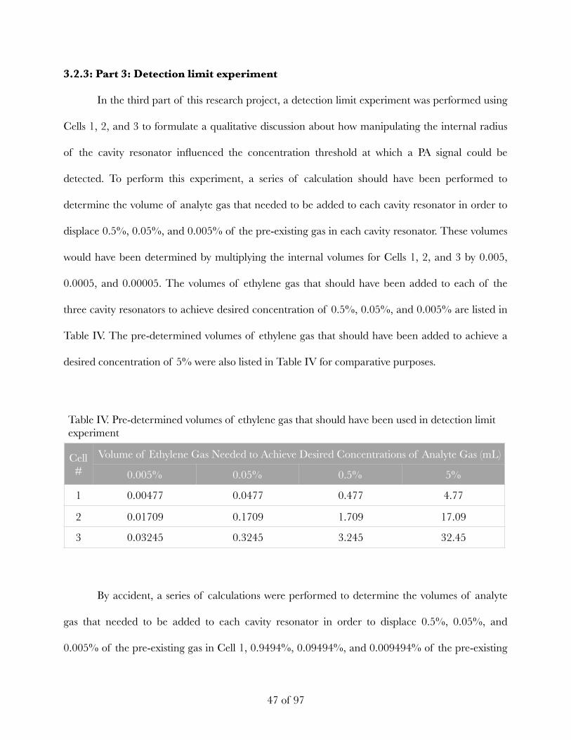
3.2.3: Part 3: Detection limit experiment

In the third part of this research project, a detection limit experiment was performed using

Cells 1, 2, and 3 to formulate a qualitative discussion about how manipulating the internal radius

of the cavity resonator influenced the concentration threshold at which a PA signal could be

detected. To perform this experiment, a series of calculation should have been performed to

determine the volume of analyte gas that needed to be added to each cavity resonator in order to

displace 0.5%, 0.05%, and 0.005% of the pre-existing gas in each cavity resonator. These volumes

would have been determined by multiplying the internal volumes for Cells 1, 2, and 3 by 0.005,

0.0005, and 0.00005. The volumes of ethylene gas that should have been added to each of the

three cavity resonators to achieve desired concentration of 0.5%, 0.05%, and 0.005% are listed in

Table IV. The pre-determined volumes of ethylene gas that should have been added to achieve a

desired concentration of 5% were also listed in Table IV for comparative purposes.

By accident, a series of calculations were performed to determine the volumes of analyte

gas that needed to be added to each cavity resonator in order to displace 0.5%, 0.05%, and

0.005% of the pre-existing gas in Cell 1, 0.9494%, 0.09494%, and 0.009494% of the pre-existing

Table IV. Pre-determined volumes of ethylene gas that should have been used in detection limit experiment

Cell #

Volume of Ethylene Gas Needed to Achieve Desired Concentrations of Analyte Gas (mL)

0.005% 0.05% 0.5% 5%

1 0.00477 0.0477 0.477 4.77

2 0.01709 0.1709 1.709 17.09

3 0.03245 0.3245 3.245 32.45

! of !47 97

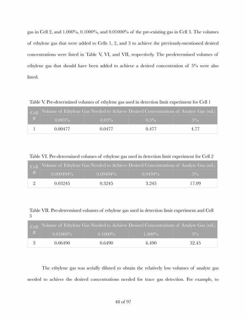
gas in Cell 2, and 1.000%, 0.1000%, and 0.01000% of the pre-existing gas in Cell 3. The volumes

of ethylene gas that were added to Cells 1, 2, and 3 to achieve the previously-mentioned desired

concentrations were listed in Table V, VI, and VII, respectively. The predetermined volumes of

ethylene gas that should have been added to achieve a desired concentration of 5% were also

listed.

The ethylene gas was serially diluted to obtain the relatively low volumes of analyte gas

needed to achieve the desired concentrations needed for trace gas detection. For example, to

Table V. Pre-determined volumes of ethylene gas used in detection limit experiment for Cell 1

Cell #

Volume of Ethylene Gas Needed to Achieve Desired Concentrations of Analyte Gas (mL)

0.005% 0.05% 0.5% 5%

1 0.00477 0.0477 0.477 4.77

Table VI. Pre-determined volumes of ethylene gas used in detection limit experiment for Cell 2

Cell #

Volume of Ethylene Gas Needed to Achieve Desired Concentrations of Analyte Gas (mL)

0.009494% 0.09494% 0.9494% 5%

2 0.03245 0.3245 3.245 17.09

Table VII. Pre-determined volumes of ethylene gas used in detection limit experiment and Cell 3

Cell #

Volume of Ethylene Gas Needed to Achieve Desired Concentrations of Analyte Gas (mL)

0.01000% 0.1000% 1.000% 5%

3 0.06490 0.6490 6.490 32.45

! of !48 97

collect and dispense 0.00477 mL of ethylene gas, a 10 mL syringe was filled with 1 mL of ethylene

gas and 9 mL of air to produce a 10 mL ethylene-air solution with a concentration of 0.1 mL

ethylene gas per mL ethylene-air solution. After allowing the ethylene-air solution to equilibrate

within the 10 mL syringe, 9 mL of the gas solution was dispensed, and the syringe was filled once

more with 9 mL of air to produce a 10 mL ethylene-air solution with a concentration of 0.01 mL

ethylene gas per mL ethylene-air solution. 4.77 ml of this ethylene-air solution was dispensed into

Cell 1 to achieve a desired concentration of 0.005%. This procedure was repeated for Cells 1, 2,

and 3 to achieve the gas concentrations needed for use in the detection limit experiment.

The data sets obtained in the second part of this research project were used to help

generate some of the spectra necessary for this part of the research project. In particular, the data

sets obtained upon reevaluation of the peaks generated in Runs A, F, and K were used to

determine the range of rotational frequencies that needed to be analyzed for determination of the

detection limit for each cavity resonator. Based on the data obtained in the second part of this

experiment, the exact rotational frequencies that produced peaks with the greatest amplitudes

when Cells 1, 2, and 3 contained 5% ethylene gas by volume were determined to be 292 Hz, 510

Hz, and 237 Hz, respectively. The rotational frequency was scanned across a 12 Hz range around

292 Hz in increments of 2 Hz to determine the intensities of the PA signal when Cell 1 contained

0.50%, 0.05%, and 0.005% ethylene gas by volume. This process was performed twice more using

510 Hz and 237 Hz (versus 292 Hz) for Cells 2 and 3, respectively. Each data set obtained was

used to create a spectrum of the intensity of the PA signal (in mV) versus the rotational frequency

(in Hz).

! of !49 97

Chapter 4: Results and Analysis

Table of Contents

• 4.1: Infrared spectra for ethylene and nitrogen

• 4.2: Experimental runs with manipulated parameters

• 4.3: Detection limit experiment

4.1: Infrared spectra of ethylene and nitrogen

The IR spectrum of ethylene gas can be found in Figure VI. The absorption wavelength of

ethylene gas was experimentally determined to exist around the wavelength 10.6 μm.

! of !50 97

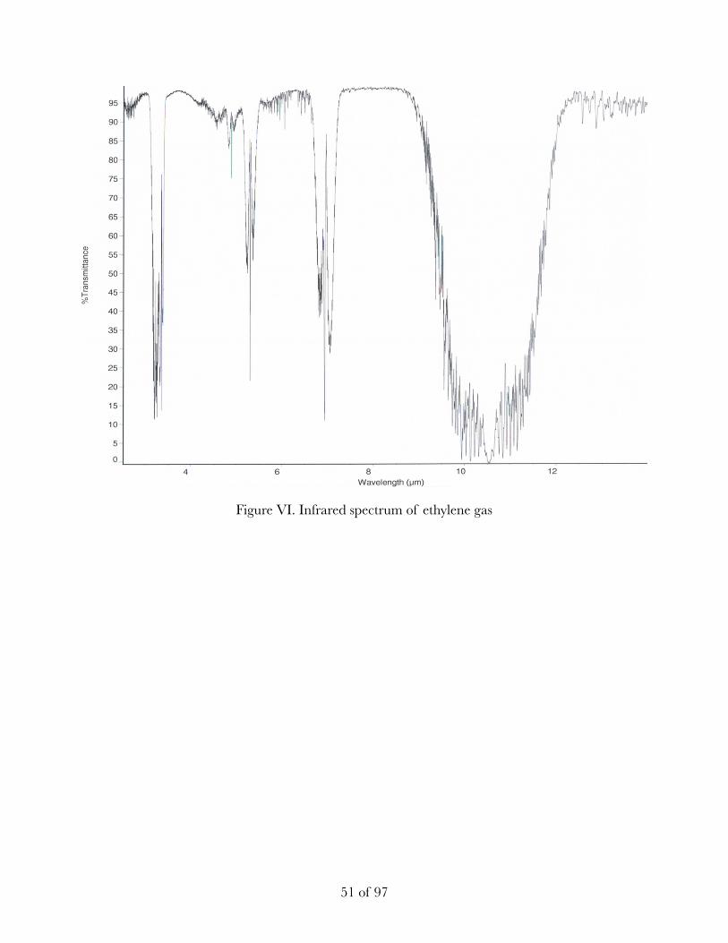
Figure VI. Infrared spectrum of ethylene gas

! of !51 97

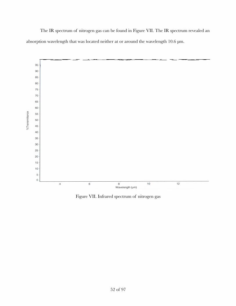
The IR spectrum of nitrogen gas can be found in Figure VII. The IR spectrum revealed an

absorption wavelength that was located neither at or around the wavelength 10.6 μm.

Figure VII. Infrared spectrum of nitrogen gas

! of !52 97

4.2: Experimental runs with manipulated parameters

A summary of the experimental runs performed in this part of the research project can be

found in Table III. The data sets obtained from Runs A - O were used to create spectra of the

intensity of the PA signal (in mV) versus the rotational frequency (in Hz). Each peak observed in

each of the aforementioned spectra was reevaluated to determine the exact values for the

rotational frequencies that produced these peaks. Hereafter, Run A2 refers to the data set obtained

upon reevaluation of the spectra generated from Run A, Run B2 refers to the data set obtained

upon reevaluation of the spectra generated from Run B, Run C2 refers to the data set obtained

upon reevaluation of the spectra generated from Run C, and so forth. The data sets obtained from

Runs A2 - O2 were also used to create spectra of the intensity of the PA signal (in mV) versus the

rotational frequency (in Hz) but only in cases where a sinusoidal wave function was observed on

the oscilloscope. The spectra for Runs A2 - O2 can also be found below. Not all peaks observed

upon initial evaluation of the spectra for Runs A - O were re-observed upon evaluation of the

spectra for Runs A2 - O2; therefore, to help maintain the integrity of the data sets gathered in this

research project that will later be used to help formulate a discussion about the PA effect of

ethylene, the spectra for Runs A - O can also be found below.

The spectra for Runs A - E were superimposed to help visualize how the intensity of the PA

signal changed as the concentration of analyte gas contained within Cell 1 was manipulated. Note

that the internal radius of the cavity resonator was held constant for Runs A - E. The resulting

spectrum can be found below in Figure VIII. For Run A, peaks were observed at rotational

frequencies of approximately 290 Hz, 560 Hz, 680 Hz, 1130 Hz, 1535 Hz, 1860 Hz, and 2155

Hz. For Run B, peaks were observed at rotational frequencies of approximately 290 Hz, 680 Hz,

1130 Hz, 1540 Hz, and 1860 Hz. For Run C, peaks were observed at rotational frequencies of

! of !53 97

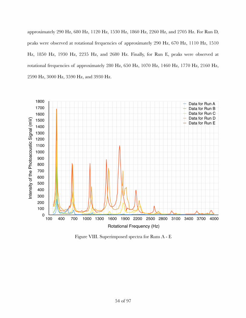
approximately 290 Hz, 680 Hz, 1120 Hz, 1530 Hz, 1860 Hz, 2260 Hz, and 2705 Hz. For Run D,

peaks were observed at rotational frequencies of approximately 290 Hz, 670 Hz, 1110 Hz, 1510

Hz, 1850 Hz, 1930 Hz, 2235 Hz, and 2680 Hz. Finally, for Run E, peaks were observed at

rotational frequencies of approximately 280 Hz, 650 Hz, 1070 Hz, 1460 Hz, 1770 Hz, 2160 Hz,

2590 Hz, 3000 Hz, 3590 Hz, and 3930 Hz.

Figure VIII. Superimposed spectra for Runs A - E

! of !54 97

Inte

nsity

of t

he P

hoto

acou

stic

Sig

nal (

mV)

0100200300400500600700800900

100011001200130014001500160017001800

Rotational Frequency (Hz)100 400 700 1000 1300 1600 1900 2200 2500 2800 3100 3400 3700 4000

Data for Run AData for Run BData for Run CData for Run DData for Run E

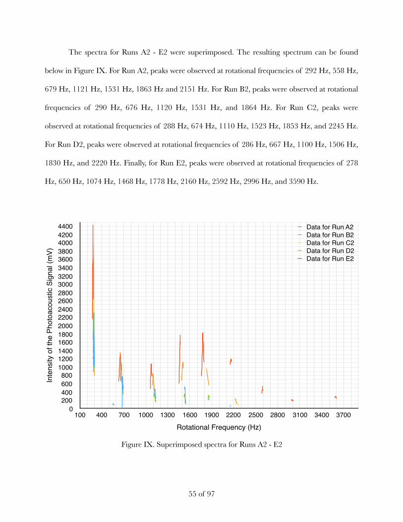
The spectra for Runs A2 - E2 were superimposed. The resulting spectrum can be found

below in Figure IX. For Run A2, peaks were observed at rotational frequencies of 292 Hz, 558 Hz,

679 Hz, 1121 Hz, 1531 Hz, 1863 Hz and 2151 Hz. For Run B2, peaks were observed at rotational

frequencies of 290 Hz, 676 Hz, 1120 Hz, 1531 Hz, and 1864 Hz. For Run C2, peaks were

observed at rotational frequencies of 288 Hz, 674 Hz, 1110 Hz, 1523 Hz, 1853 Hz, and 2245 Hz.

For Run D2, peaks were observed at rotational frequencies of 286 Hz, 667 Hz, 1100 Hz, 1506 Hz,

1830 Hz, and 2220 Hz. Finally, for Run E2, peaks were observed at rotational frequencies of 278

Hz, 650 Hz, 1074 Hz, 1468 Hz, 1778 Hz, 2160 Hz, 2592 Hz, 2996 Hz, and 3590 Hz.

Figure IX. Superimposed spectra for Runs A2 - E2

! of !55 97

Inte

nsity

of t

he P

hoto

acou

stic

Sig

nal (

mV)

0200400600800

100012001400160018002000220024002600280030003200340036003800400042004400

Rotational Frequency (Hz)100 400 700 1000 1300 1600 1900 2200 2500 2800 3100 3400 3700

Data for Run A2Data for Run B2Data for Run C2Data for Run D2Data for Run E2

The spectra for Runs F - J were superimposed to help visualize how the intensity of the PA

signal changed as the concentration of analyte gas contained within Cell 2 was manipulated. Note

that the internal radius of the cavity resonator was held constant for Runs F - J. The resulting

spectrum can be found below in Figure X. For Run F, peaks were observed at rotational

frequencies of approximately 310 Hz, 510 Hz, 710 Hz, and 1320 Hz. For Run G, peaks were

observed at rotational frequencies of approximately 300 Hz, 510 Hz, 720 Hz, and 2470 Hz. For

Run H, peaks were observed at rotational frequencies of approximately 325 Hz, 510 Hz, 720 Hz,

1920 Hz, and 2500 Hz. For Run I, peaks were observed at rotational frequencies of approximately

380 Hz, 500 Hz, 710 Hz, 1910 Hz, 2450 Hz, and 2760 Hz. Finally, for Run J, peaks were observed

at rotational frequencies of approximately 380 Hz, 490 Hz, 680 Hz, 2340 Hz, 2625 Hz and 3840

Hz.

! of !56 97

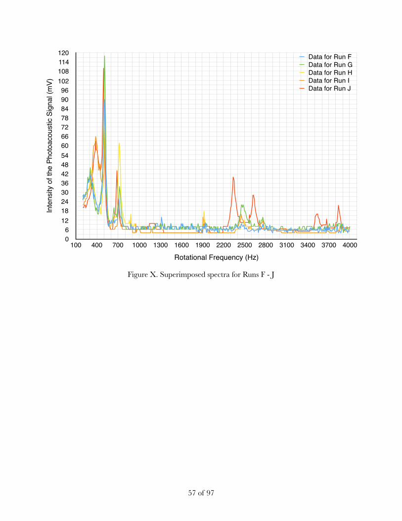
Figure X. Superimposed spectra for Runs F - J

! of !57 97

Inte

nsity

of t

he P

hoto

acou

stic

Sig

nal (

mV)

06

121824303642485460667278849096

102108114120

Rotational Frequency (Hz)100 400 700 1000 1300 1600 1900 2200 2500 2800 3100 3400 3700 4000

Data for Run FData for Run GData for Run HData for Run IData for Run J

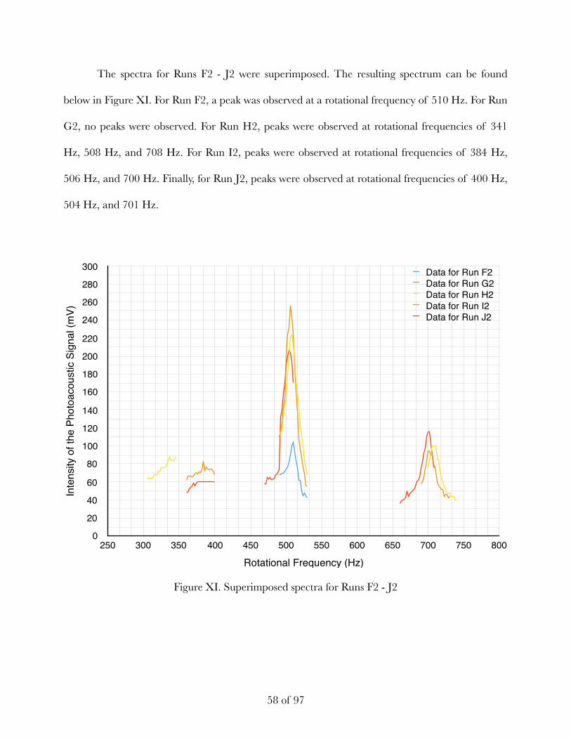
The spectra for Runs F2 - J2 were superimposed. The resulting spectrum can be found

below in Figure XI. For Run F2, a peak was observed at a rotational frequency of 510 Hz. For Run

G2, no peaks were observed. For Run H2, peaks were observed at rotational frequencies of 341

Hz, 508 Hz, and 708 Hz. For Run I2, peaks were observed at rotational frequencies of 384 Hz,

506 Hz, and 700 Hz. Finally, for Run J2, peaks were observed at rotational frequencies of 400 Hz,

504 Hz, and 701 Hz.

Figure XI. Superimposed spectra for Runs F2 - J2

! of !58 97

Inte

nsity

of t

he P

hoto

acou

stic

Sig

nal (

mV)

0

20

40

60

80

100

120

140

160

180

200

220

240

260

280

300

Rotational Frequency (Hz)250 300 350 400 450 500 550 600 650 700 750 800

Data for Run F2Data for Run G2Data for Run H2Data for Run I2Data for Run J2

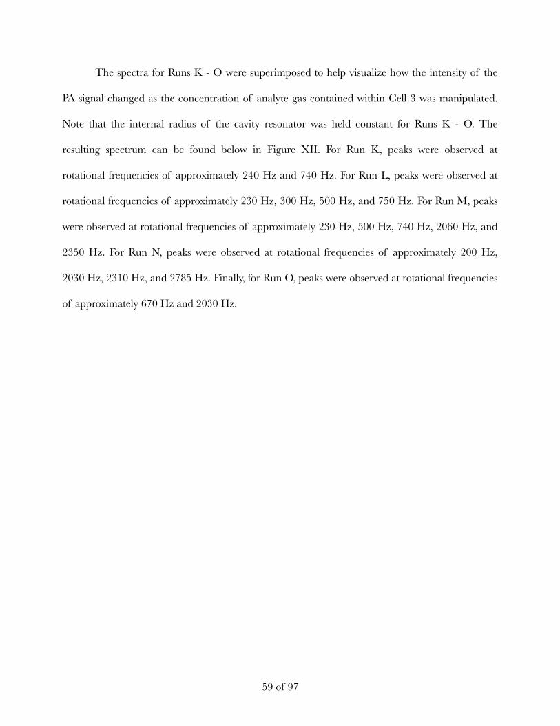
The spectra for Runs K - O were superimposed to help visualize how the intensity of the

PA signal changed as the concentration of analyte gas contained within Cell 3 was manipulated.

Note that the internal radius of the cavity resonator was held constant for Runs K - O. The

resulting spectrum can be found below in Figure XII. For Run K, peaks were observed at

rotational frequencies of approximately 240 Hz and 740 Hz. For Run L, peaks were observed at

rotational frequencies of approximately 230 Hz, 300 Hz, 500 Hz, and 750 Hz. For Run M, peaks

were observed at rotational frequencies of approximately 230 Hz, 500 Hz, 740 Hz, 2060 Hz, and

2350 Hz. For Run N, peaks were observed at rotational frequencies of approximately 200 Hz,

2030 Hz, 2310 Hz, and 2785 Hz. Finally, for Run O, peaks were observed at rotational frequencies

of approximately 670 Hz and 2030 Hz.

! of !59 97

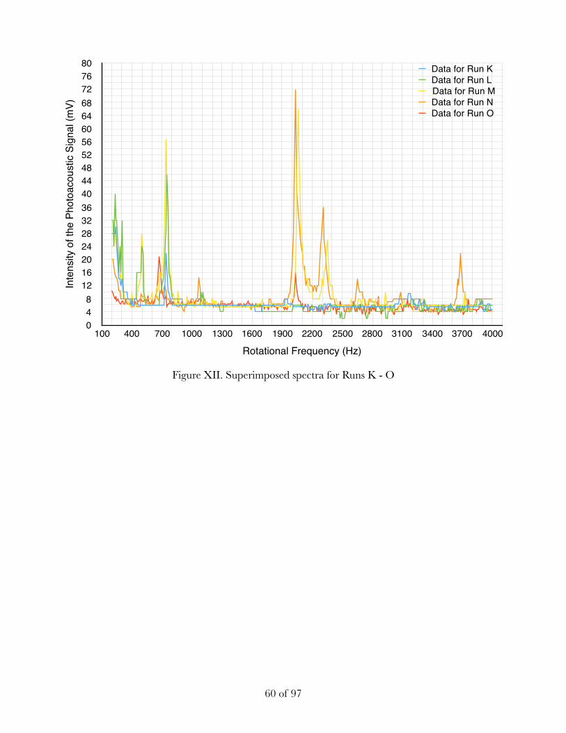
Figure XII. Superimposed spectra for Runs K - O

! of !60 97

Inte

nsity

of t

he P

hoto

acou

stic

Sig

nal (

mV)

048

121620242832364044485256606468727680

Rotational Frequency (Hz)100 400 700 1000 1300 1600 1900 2200 2500 2800 3100 3400 3700 4000

Data for Run KData for Run LData for Run M Data for Run NData for Run O

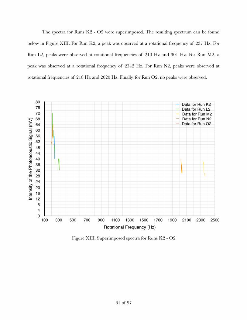
The spectra for Runs K2 - O2 were superimposed. The resulting spectrum can be found

below in Figure XIII. For Run K2, a peak was observed at a rotational frequency of 237 Hz. For

Run L2, peaks were observed at rotational frequencies of 210 Hz and 301 Hz. For Run M2, a

peak was observed at a rotational frequency of 2342 Hz. For Run N2, peaks were observed at

rotational frequencies of 218 Hz and 2020 Hz. Finally, for Run O2, no peaks were observed.

Figure XIII. Superimposed spectra for Runs K2 - O2

! of !61 97

Inte

nsity

of t

he P

hoto

acou

stic

Sig

nal (

mV)

048

121620242832364044485256606468727680

Rotational Frequency (Hz)100 300 500 700 900 1100 1300 1500 1700 1900 2100 2300 2500

Data for Run K2Data for Run L2Data for Run M2 Data for Run N2 Data for Run O2

The spectra for Runs A, F, and K were superimposed to help visualize how the intensity of

the PA signal changed when the internal radius of the cavity resonator was manipulated but the

concentration of analyte gas contained within each cavity resonator was held constant at 5%. The

resulting spectrum can be found below in Figure XIV.

Figure XIV. Superimposed spectra for Runs A, F, K

! of !62 97

Inte

nsity

of t

he P

hoto

acou

stic

Sig

nal (

mV)

0

20

40

60

80

100

120

140

160

180

200

220

240

Rotational Frequency (Hz)100 400 700 1000 1300 1600 1900 2200 2500 2800 3100 3400 3700 4000

Data for Run AData for Run FData for Run K

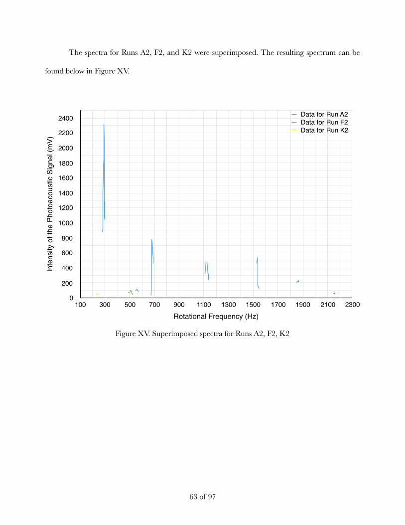
The spectra for Runs A2, F2, and K2 were superimposed. The resulting spectrum can be

found below in Figure XV.

Figure XV. Superimposed spectra for Runs A2, F2, K2

! of !63 97

Inte

nsity

of t

he P

hoto

acou

stic

Sig

nal (

mV)

0

200

400

600

800

1000

1200

1400

1600

1800

2000

2200

2400

Rotational Frequency (Hz)100 300 500 700 900 1100 1300 1500 1700 1900 2100 2300

Data for Run A2Data for Run F2Data for Run K2

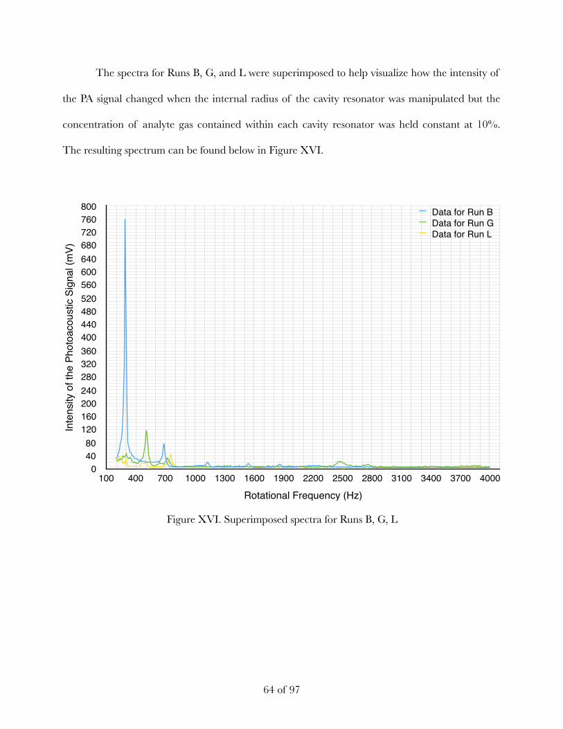
The spectra for Runs B, G, and L were superimposed to help visualize how the intensity of

the PA signal changed when the internal radius of the cavity resonator was manipulated but the

concentration of analyte gas contained within each cavity resonator was held constant at 10%.

The resulting spectrum can be found below in Figure XVI.

Figure XVI. Superimposed spectra for Runs B, G, L

! of !64 97

Inte

nsity

of t

he P

hoto

acou

stic

Sig

nal (

mV)

04080

120160200240280320360400440480520560600640680720760800

Rotational Frequency (Hz)100 400 700 1000 1300 1600 1900 2200 2500 2800 3100 3400 3700 4000

Data for Run BData for Run GData for Run L

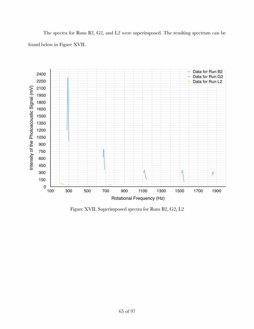
The spectra for Runs B2, G2, and L2 were superimposed. The resulting spectrum can be

found below in Figure XVII.

Figure XVII. Superimposed spectra for Runs B2, G2, L2

! of !65 97

Inte

nsity

of t

he P

hoto

acou

stic

Sig

nal (

mV)

0150300450600750900

1050120013501500165018001950210022502400

Rotational Frequency (Hz)100 300 500 700 900 1100 1300 1500 1700 1900

Data for Run B2Data for Run G2Data for Run L2

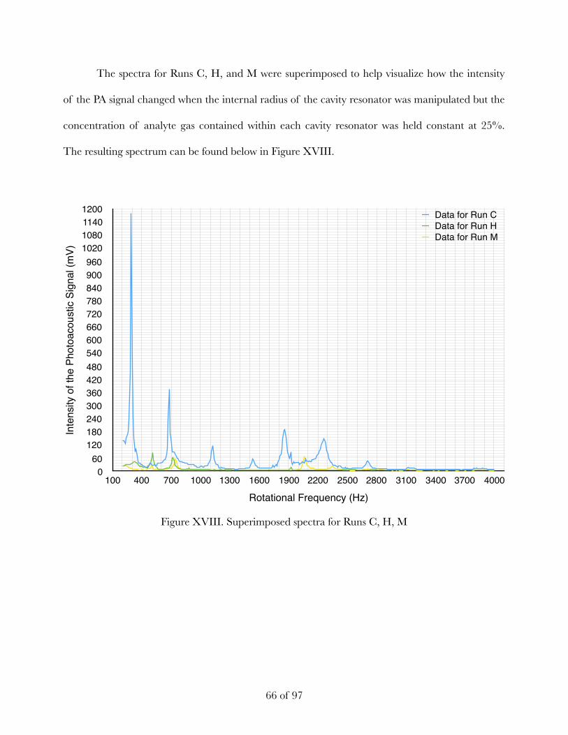
The spectra for Runs C, H, and M were superimposed to help visualize how the intensity

of the PA signal changed when the internal radius of the cavity resonator was manipulated but the

concentration of analyte gas contained within each cavity resonator was held constant at 25%.

The resulting spectrum can be found below in Figure XVIII.

Figure XVIII. Superimposed spectra for Runs C, H, M

! of !66 97

Inte

nsity

of t

he P

hoto

acou

stic

Sig

nal (

mV)

060

120180240300360420480540600660720780840900960

1020108011401200

Rotational Frequency (Hz)100 400 700 1000 1300 1600 1900 2200 2500 2800 3100 3400 3700 4000

Data for Run CData for Run HData for Run M

The spectra for Runs C2, H2, and M2 were superimposed. The resulting spectrum can be

found below in Figure XIX.

Figure XIX. Superimposed spectra for Runs C2, H2, M2

! of !67 97

Inte

nsity

of t

he P

hoto

acou

stic

Sig

nal (

mV)

0150300450600750900

105012001350150016501800195021002250240025502700

Rotational Frequency (Hz)100 300 500 700 900 1100 1300 1500 1700 1900 2100 2300 2500

Data for Run C2Data for Run H2Data for Run M2

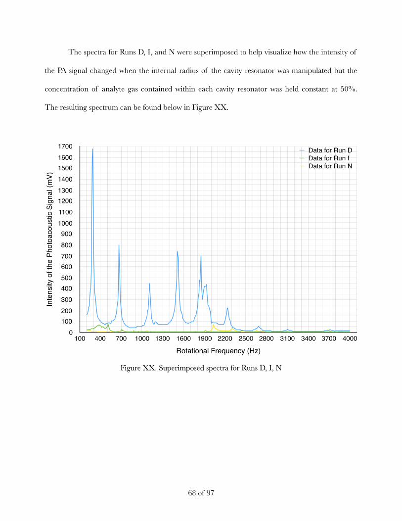
The spectra for Runs D, I, and N were superimposed to help visualize how the intensity of

the PA signal changed when the internal radius of the cavity resonator was manipulated but the

concentration of analyte gas contained within each cavity resonator was held constant at 50%.

The resulting spectrum can be found below in Figure XX.

Figure XX. Superimposed spectra for Runs D, I, N

! of !68 97

Inte

nsity

of t

he P

hoto

acou

stic

Sig

nal (

mV)

0100200300400500600700800900

10001100120013001400150016001700

Rotational Frequency (Hz)100 400 700 1000 1300 1600 1900 2200 2500 2800 3100 3400 3700 4000

Data for Run DData for Run IData for Run N

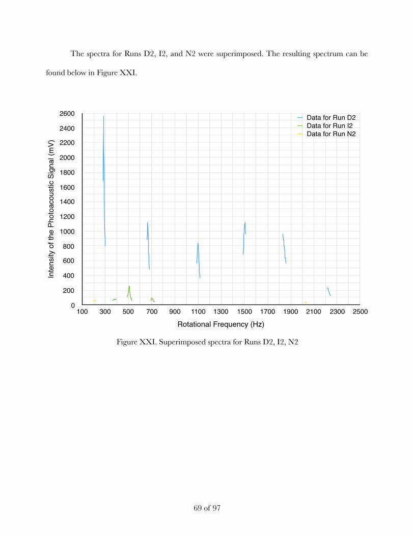
The spectra for Runs D2, I2, and N2 were superimposed. The resulting spectrum can be

found below in Figure XXI.

Figure XXI. Superimposed spectra for Runs D2, I2, N2

! of !69 97

Inte

nsity

of t

he P

hoto

acou

stic

Sig

nal (

mV)

0

200

400

600

800

1000

1200

1400

1600

1800

2000

2200

2400

2600

Rotational Frequency (Hz)100 300 500 700 900 1100 1300 1500 1700 1900 2100 2300 2500

Data for Run D2Data for Run I2Data for Run N2

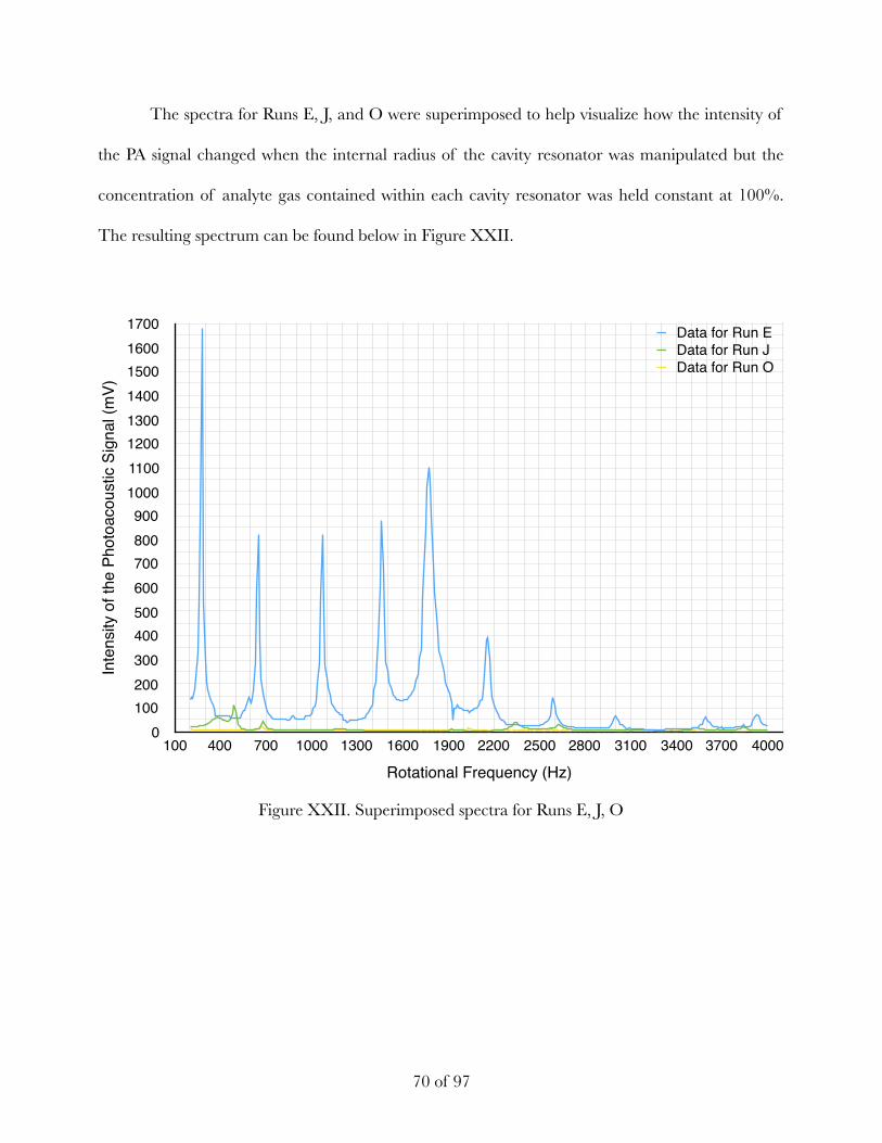
The spectra for Runs E, J, and O were superimposed to help visualize how the intensity of

the PA signal changed when the internal radius of the cavity resonator was manipulated but the

concentration of analyte gas contained within each cavity resonator was held constant at 100%.

The resulting spectrum can be found below in Figure XXII.

Figure XXII. Superimposed spectra for Runs E, J, O

! of !70 97

Inte

nsity

of t

he P

hoto

acou

stic

Sig

nal (

mV)

0100200300400500600700800900

10001100120013001400150016001700

Rotational Frequency (Hz)100 400 700 1000 1300 1600 1900 2200 2500 2800 3100 3400 3700 4000

Data for Run EData for Run JData for Run O

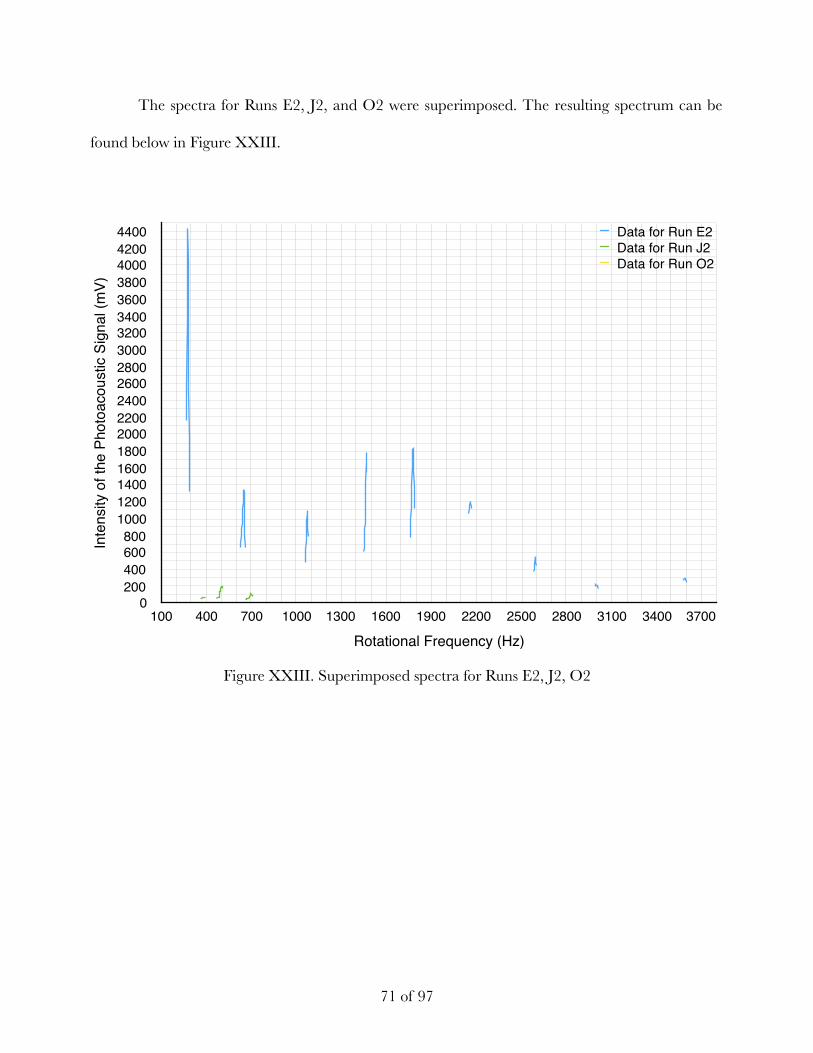
The spectra for Runs E2, J2, and O2 were superimposed. The resulting spectrum can be

found below in Figure XXIII.

Figure XXIII. Superimposed spectra for Runs E2, J2, O2

! of !71 97

Inte

nsity

of t

he P

hoto

acou

stic

Sig

nal (

mV)

0200400600800

100012001400160018002000220024002600280030003200340036003800400042004400

Rotational Frequency (Hz)100 400 700 1000 1300 1600 1900 2200 2500 2800 3100 3400 3700

Data for Run E2Data for Run J2Data for Run O2

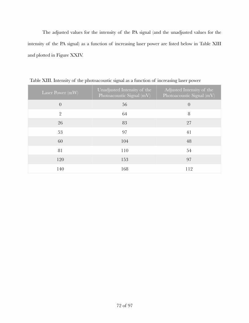
The adjusted values for the intensity of the PA signal (and the unadjusted values for the

intensity of the PA signal) as a function of increasing laser power are listed below in Table XIII

and plotted in Figure XXIV.

Table XIII. Intensity of the photoacoustic signal as a function of increasing laser power

Laser Power (mW) Unadjusted Intensity of the Photoacoustic Signal (mV)

Adjusted Intensity of the Photoacoustic Signal (mV)

0 56 0

2 64 8

26 83 27

53 97 41

60 104 48

81 110 54

120 153 97

140 168 112

! of !72 97

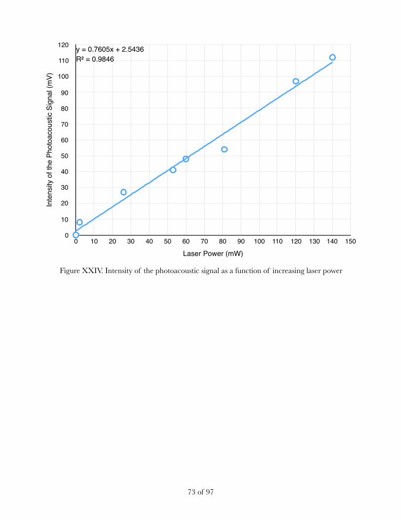
Figure XXIV. Intensity of the photoacoustic signal as a function of increasing laser power

! of !73 97

Inte

nsity

of t

he P

hoto

acou

stic

Sig

nal (

mV)

0

10

20

30

40

50

60

70

80

90

100

110

120

Laser Power (mW)0 10 20 30 40 50 60 70 80 90 100 110 120 130 140 150

y = 0.7605x + 2.5436R² = 0.9846

4.3: Detection limit experiment

The volumes of ethylene gas needed to achieve desired concentrations of 5%, 0.5%,

0.05%, and 0.005% for Cell 1, 5%, 0.9494%, 0.09494%, and 0.009494% for Cell 2, and 5%, 1%,

0.1%, and 0.01% for Cell 3 are listed in Tables V, VI, and VII, respectively. The data sets obtained

were used to create spectra of the intensity of the PA signal (in mV) versus the rotational frequency

(in Hz). The four spectra generated for Cell 1 in this part of the research project were

superimposed to help visualize how the intensity of the PA signal changed when the concentration

of ethylene gas contained within Cell 1 was manipulated. Note that the internal radius of the

cavity resonator was held constant. The resulting spectra can be found in Figures XXV and

XXVI.

! of !74 97

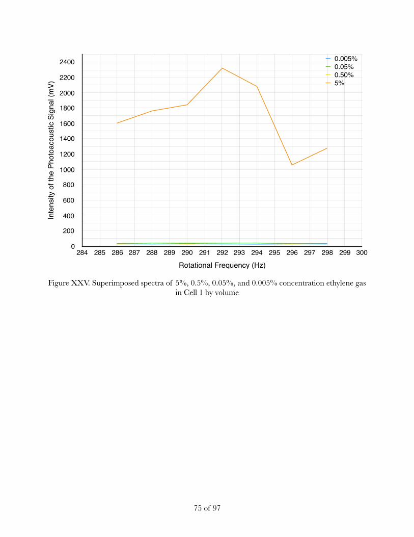
Figure XXV. Superimposed spectra of 5%, 0.5%, 0.05%, and 0.005% concentration ethylene gas in Cell 1 by volume

! of !75 97

Inte

nsity

of t

he P

hoto

acou

stic

Sig

nal (

mV)

0

200

400

600

800

1000

1200

1400

1600

1800

2000

2200

2400

Rotational Frequency (Hz)284 285 286 287 288 289 290 291 292 293 294 295 296 297 298 299 300

0.005%0.05%0.50%5%

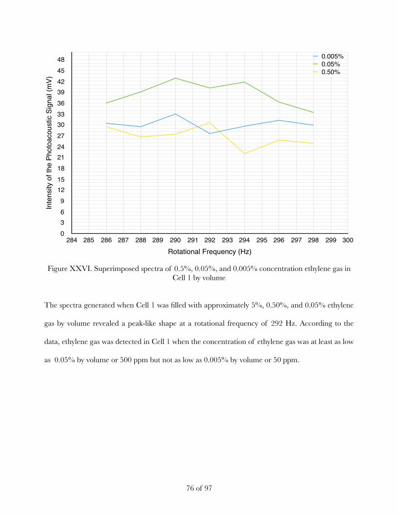
Figure XXVI. Superimposed spectra of 0.5%, 0.05%, and 0.005% concentration ethylene gas in Cell 1 by volume

The spectra generated when Cell 1 was filled with approximately 5%, 0.50%, and 0.05% ethylene

gas by volume revealed a peak-like shape at a rotational frequency of 292 Hz. According to the

data, ethylene gas was detected in Cell 1 when the concentration of ethylene gas was at least as low

as 0.05% by volume or 500 ppm but not as low as 0.005% by volume or 50 ppm.

! of !76 97

Inte

nsity

of t

he P

hoto

acou

stic

Sig

nal (

mV)

0369

12151821242730333639424548

Rotational Frequency (Hz)284 285 286 287 288 289 290 291 292 293 294 295 296 297 298 299 300

0.005%0.05%0.50%

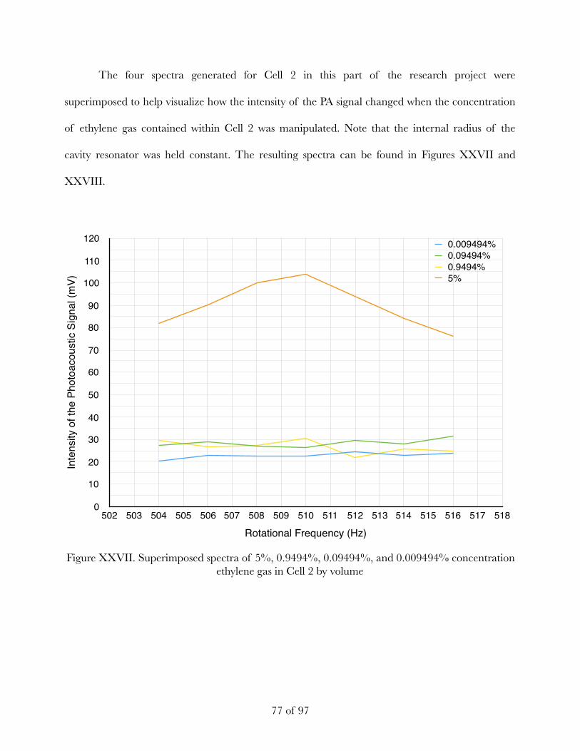
The four spectra generated for Cell 2 in this part of the research project were

superimposed to help visualize how the intensity of the PA signal changed when the concentration

of ethylene gas contained within Cell 2 was manipulated. Note that the internal radius of the

cavity resonator was held constant. The resulting spectra can be found in Figures XXVII and

XXVIII.

Figure XXVII. Superimposed spectra of 5%, 0.9494%, 0.09494%, and 0.009494% concentration ethylene gas in Cell 2 by volume

! of !77 97

Inte

nsity

of t

he P

hoto

acou

stic

Sig

nal (

mV)

0

10

20

30

40

50

60

70

80

90

100

110

120

Rotational Frequency (Hz)502 503 504 505 506 507 508 509 510 511 512 513 514 515 516 517 518

0.009494%0.09494%0.9494%5%

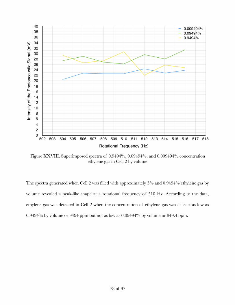
Figure XXVIII. Superimposed spectra of 0.9494%, 0.09494%, and 0.009494% concentration ethylene gas in Cell 2 by volume

The spectra generated when Cell 2 was filled with approximately 5% and 0.9494% ethylene gas by

volume revealed a peak-like shape at a rotational frequency of 510 Hz. According to the data,

ethylene gas was detected in Cell 2 when the concentration of ethylene gas was at least as low as

0.9494% by volume or 9494 ppm but not as low as 0.09494% by volume or 949.4 ppm.

! of !78 97

Inte

nsity

of t

he P

hoto

acou

stic

Sig

nal (

mV)

02468

10121416182022242628303234363840

Rotational Frequency (Hz)502 503 504 505 506 507 508 509 510 511 512 513 514 515 516 517 518

0.009494%0.09494%0.9494%

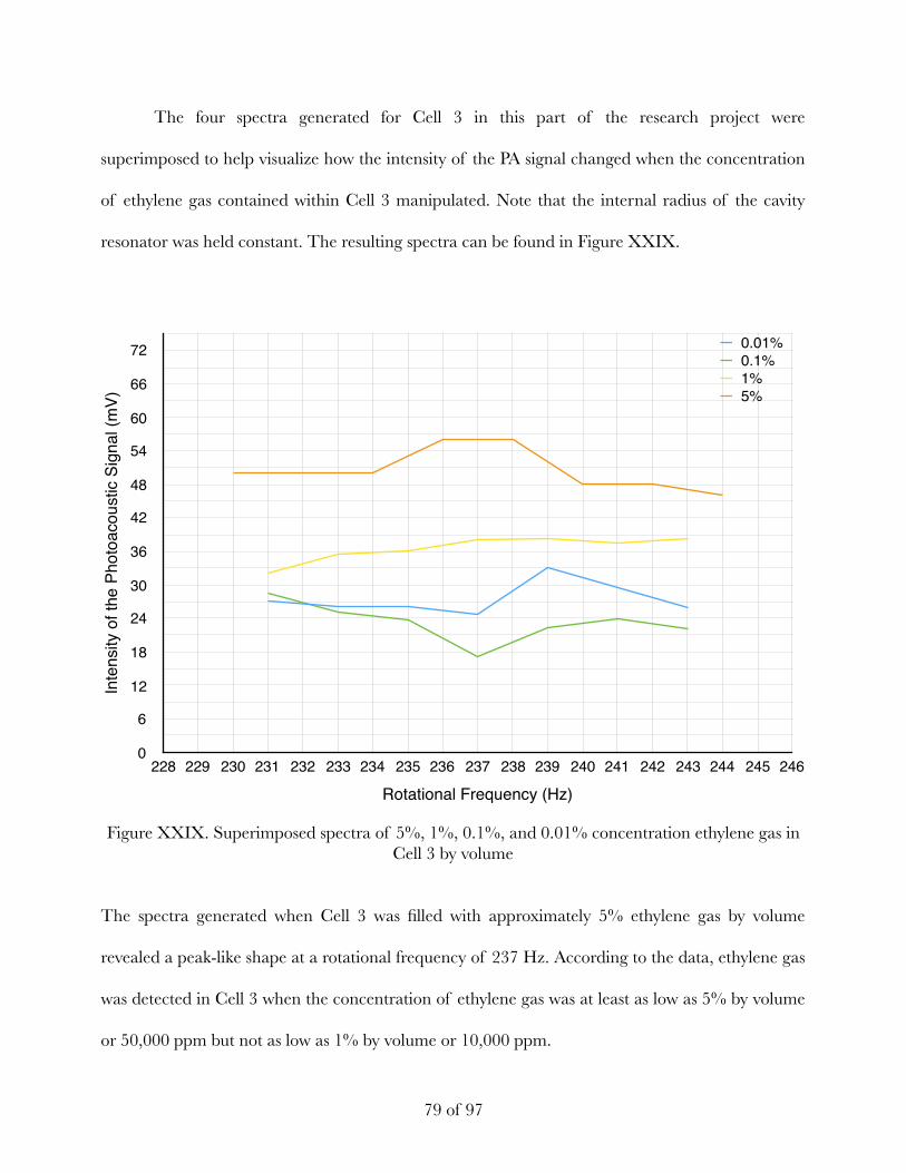
The four spectra generated for Cell 3 in this part of the research project were

superimposed to help visualize how the intensity of the PA signal changed when the concentration

of ethylene gas contained within Cell 3 manipulated. Note that the internal radius of the cavity

resonator was held constant. The resulting spectra can be found in Figure XXIX.

Figure XXIX. Superimposed spectra of 5%, 1%, 0.1%, and 0.01% concentration ethylene gas in Cell 3 by volume

The spectra generated when Cell 3 was filled with approximately 5% ethylene gas by volume

revealed a peak-like shape at a rotational frequency of 237 Hz. According to the data, ethylene gas

was detected in Cell 3 when the concentration of ethylene gas was at least as low as 5% by volume

or 50,000 ppm but not as low as 1% by volume or 10,000 ppm.

! of !79 97

Inte

nsity

of t

he P

hoto

acou

stic

Sig

nal (

mV)

0

6

12

18

24

30

36

42

48

54

60

66

72

Rotational Frequency (Hz)228 229 230 231 232 233 234 235 236 237 238 239 240 241 242 243 244 245 246

0.01%0.1%1%5%

Chapter 5: Discussion

Table of Contents

• 5.1: IR spectra of ethylene and nitrogen

• 5.2: Experimental runs with manipulated parameters

• 5.3: Detection limit experiment

• 5.4: Sources of uncertainty and future research

• 5.5: Statement of results

5.1: Infrared spectra of ethylene and nitrogen

This research project was performed to help contribute to the current understanding of the

PA effect of ethylene gas. Various aspects of the experimental setup in this research project were

independently manipulated to determine each of their effects on the PA signal produced by

ethylene.

First and foremost, IR spectroscopy technique was utilized to verify that use of the buffer

gas nitrogen would not interfere with detection and measurement of the analyte gas ethylene. The

IR absorption spectra for both ethylene gas and nitrogen gas were obtained and can be found in

! of !80 97

Figures VI and VII, respectively. According to Figure VI, the absorption wavelength of ethylene

was experimentally verified to exist around the wavelength 10.6 μm. Furthermore, because

ethylene was a strongly absorbing gas with a high absorption coefficient, the percent transmittance

was 0% at 10.6 μm. According to Figure VI, the absorption spectra for nitrogen revealed no

absorbance at or around 10.6 μm. This IR-inactive gas was, in fact, an appropriate buffer gas to

use in this research project. These findings were consistent with the literature findings.

5.2: Experimental runs with manipulated parameters

In the second part of this research project, four aspects of the experimental setup were

independently manipulated. These experimental parameters include the internal radius of the

cavity resonator, power of the light source, concentration of analyte gas contained within the

cavity resonator, and rotational frequency of the mechanical chopper. The spectra found in

Chapter 4: Results, generated by superimposing the previously-obtained spectra for Runs A - O

and Runs A2 - O2, were used to help visualize how manipulation of any of these four variables

influenced the PA behavior of the analyte gas. Each spectrum used to create the superimposed

spectra in Chapter 4: Results was individually evaluated to determine if any patterns were evident.

Upon initial evaluation of all spectra generated using the data sites for Runs A - O and A2

- O2, it was determined that in some cases but not all, as the rotational frequency of the

mechanical chopper was increased, the intensities of the resulting PA resonance peaks (for spectra

where more than two peak were observed) exponentially decreased. Literature references were

used to support these findings. According to the journal article “Photoacoustic Spectroscopy for

Process Analysis” and as previously mentioned in Chapter 2: Background, as the modulation

frequency (and pulsation frequency) increases, the time in between each consecutive excitation and

! of !81 97

de-excitation decreases, resulting in pressure fluctuations that are more difficult to distinguish

among one another. Failure of the ICP transducer to detect and distinguish individual pressure

fluctuations results in PA signals with relatively small intensities (17).

Additionally, upon initial evaluation of all spectra, it was determined that in some cases but

not all, the PA resonance peaks (for spectra where more than two peaks were observed) were

spaced out along the x-axis approximately equidistant from one another. According to the data, it

was determined that PA resonance occurred at rotational frequencies with values that were

multiples (approximately) of one another. For example, according to the data set for Run E, PA

resonance occurred at rotational frequencies with values that were approximately 370 Hz apart. In

other words, as the rotational frequency of the mechanical chopper was increased in 370 Hz

increments beginning with 280 Hz, the frequency of the pressure fluctuations reflected off the

boundaries of the cavity resonator at an arbitrary point in time was in phase with the natural

frequency of the pressure fluctuations generated by the photon absorption of the analyte gas

molecules at another arbitrary point in time. The presence or absence of the previously mentioned

patterns—exponentially-decreasing intensities of the resonance peaks and evenly-spaced

resonance peaks—were both used to help formulate a discussion about the quality of the PA effect.

Experimental parameters that yielded both of the aforementioned patterns were determined to

exhibit high quality PA behavior.

The spectra obtained using the data sets for Runs A - E and Runs A2 - E2 were

superimposed to generate the spectra shown in Figures VIII and IX. These spectra were generated

to help visualize how the intensity of the PA signal changed as the rotational frequency of the

mechanical chopper and the concentration of analyte gas contained within Cell 1 were

manipulated. The internal radius of the cavity resonator and the power of the light source were

! of !82 97

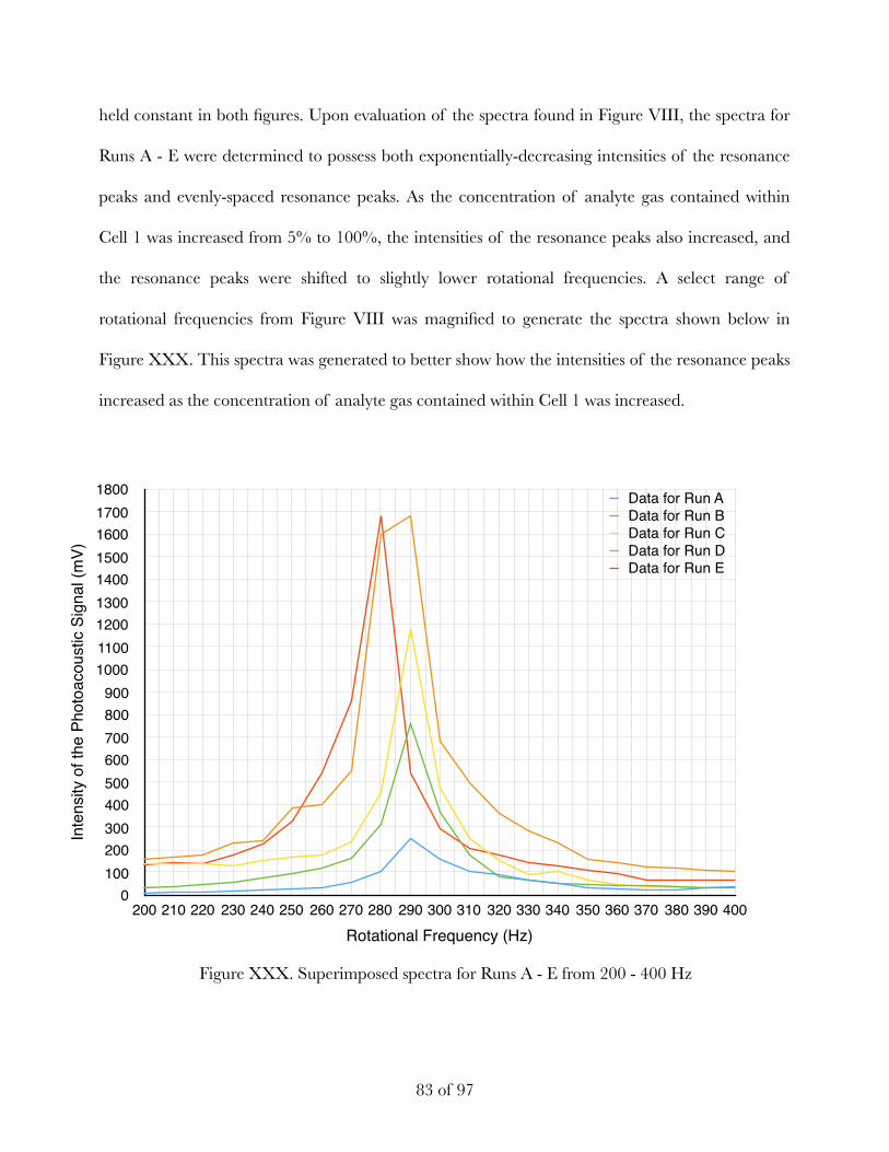
held constant in both figures. Upon evaluation of the spectra found in Figure VIII, the spectra for

Runs A - E were determined to possess both exponentially-decreasing intensities of the resonance

peaks and evenly-spaced resonance peaks. As the concentration of analyte gas contained within

Cell 1 was increased from 5% to 100%, the intensities of the resonance peaks also increased, and

the resonance peaks were shifted to slightly lower rotational frequencies. A select range of

rotational frequencies from Figure VIII was magnified to generate the spectra shown below in

Figure XXX. This spectra was generated to better show how the intensities of the resonance peaks

increased as the concentration of analyte gas contained within Cell 1 was increased.

Figure XXX. Superimposed spectra for Runs A - E from 200 - 400 Hz

! of !83 97

Inte

nsity

of t

he P

hoto

acou

stic

Sig

nal (

mV)

0100200300400500600700800900

100011001200130014001500160017001800

Rotational Frequency (Hz)200 210 220 230 240 250 260 270 280 290 300 310 320 330 340 350 360 370 380 390 400

Data for Run AData for Run BData for Run CData for Run DData for Run E

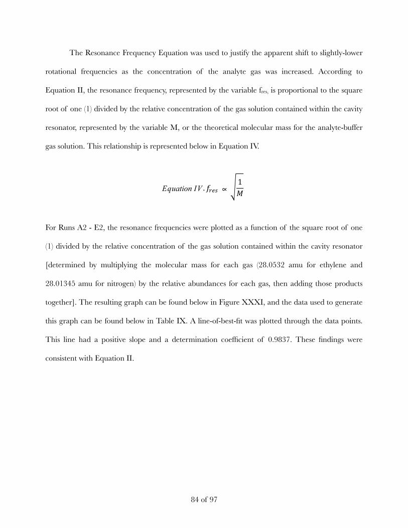
The Resonance Frequency Equation was used to justify the apparent shift to slightly-lower

rotational frequencies as the concentration of the analyte gas was increased. According to

Equation II, the resonance frequency, represented by the variable fres, is proportional to the square

root of one (1) divided by the relative concentration of the gas solution contained within the cavity

resonator, represented by the variable M, or the theoretical molecular mass for the analyte-buffer

gas solution. This relationship is represented below in Equation IV.

For Runs A2 - E2, the resonance frequencies were plotted as a function of the square root of one

(1) divided by the relative concentration of the gas solution contained within the cavity resonator

[determined by multiplying the molecular mass for each gas (28.0532 amu for ethylene and

28.01345 amu for nitrogen) by the relative abundances for each gas, then adding those products

together]. The resulting graph can be found below in Figure XXXI, and the data used to generate

this graph can be found below in Table IX. A line-of-best-fit was plotted through the data points.

This line had a positive slope and a determination coefficient of 0.9837. These findings were

consistent with Equation II.

! of !84 97

Cell # Internal Length (cm) Internal Radius (cm) Internal Volume (mL)

1 45.0 0.953 95.27 2 44.0 1.91 341.77 3 45.0 2.54 649.03

!"#$%&'(*. ,-.'(/% ∝ 12

!"#$%&'(**. 3456 = 8612; ∝ 1<=

> × 12;

!"#$%&'(***. 3456 = 1>

Cell # Volume of Ethylene Gas Needed to Achieve Desired Concentrations of Analyte Gas (mL) 5% 10% 25% 50% 100%

1 4.764 9.527 23.82 47.64 95.27 2 17.089 34.177 85.443 170.89 341.77 3 32.452 64.903 162.26 324.52 649.03

Run

Cell [Internal Radius of

Cavity Resonator

(cm)]

Concentrations of Analyte Gas Contained Within Cavity

Resonator (%) [Volume of Analyte Gas Needed to

Achieve Desired Concentrations (mL)]

Rotational Frequency of Mechanical

Chopper (Hz)

Power of Light Source (%) [Exact Power of

Light Source (mW)]

Windows

1 (0.953) 2 (1.91) 3 (2.54)

4 (unknown)

5 10 25 50

100

200 - 4000 250 100 (291.0)

(1st, 2nd) C: coated

UC: uncoated

A 1 (0.953) 5 (4.764) 200 - 4000 100 (291.0) (C, C) B 1 (0.953) 10 (9.527) 200 - 4000 100 (291.0) (C, C) C 1 (0.953) 25 (23.82) 200 - 4000 100 (291.0) (C, C) D 1 (0.953) 50 (47.64) 200 - 4000 100 (291.0) (C, C) E 1 (0.953) 100 (95.27) 200 - 4000 100 (291.0) (C, C) F 2 (1.91) 5 (17.089) 200 - 4000 100 (291.0) (C, C) G 2 (1.91) 10 (34.177) 200 - 4000 100 (291.0) (C, C) H 2 (1.91) 25 (85.443) 200 - 4000 100 (291.0) (C, C) I 2 (1.91) 50 (170.89) 200 - 4000 100 (291.0) (C, C) J 2 (1.91) 100 (341.77) 200 - 4000 100 (291.0) (C, C) K 3 (2.54) 5 (32.452) 200 - 4000 100 (291.0) (C, C) L 3 (2.54) 10 (64.903) 200 - 4000 100 (291.0) (C, C) M 3 (2.54) 25 (162.26) 200 - 4000 100 (291.0) (C, C) N 3 (2.54) 50 (324.52) 200 - 4000 100 (291.0) (C, C)

∝

quation IV . f ∝ E res √ 1M

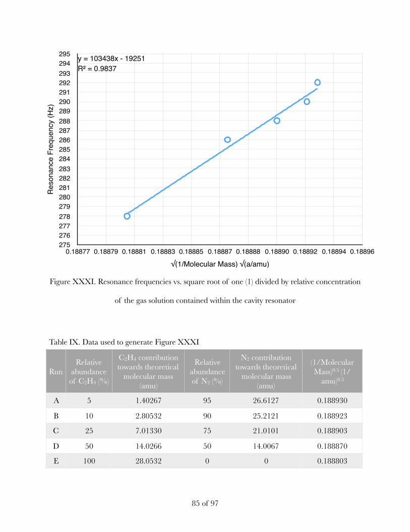
Figure XXXI. Resonance frequencies vs. square root of one (1) divided by relative concentration

of the gas solution contained within the cavity resonator

Table IX. Data used to generate Figure XXXI

RunRelative

abundance of C2H4 (%)

C2H4 contribution towards theoretical

molecular mass (amu)

Relative abundance of N2 (%)

N2 contribution towards theoretical

molecular mass (amu)

(1/Molecular Mass)0.5 (1/

amu)0.5

A 5 1.40267 95 26.6127 0.188930

B 10 2.80532 90 25.2121 0.188923

C 25 7.01330 75 21.0101 0.188903

D 50 14.0266 50 14.0067 0.188870

E 100 28.0532 0 0 0.188803

! of !85 97

Res

onan

ce F

requ

ency

(Hz)

275276277278279280281282283284285286287288289290291292293294295

√(1/Molecular Mass) √(a/amu)0.18877 0.18879 0.18881 0.18883 0.18885 0.18887 0.18888 0.18890 0.18892 0.18894 0.18896

y = 103438x - 19251R² = 0.9837

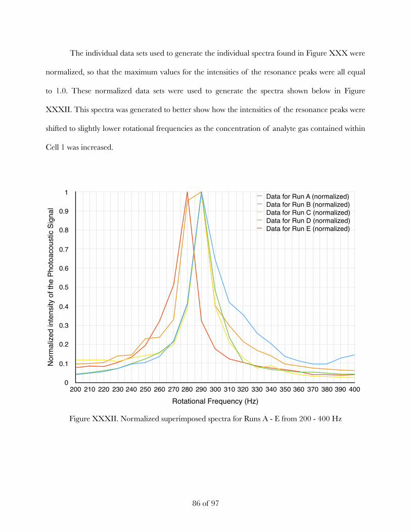
The individual data sets used to generate the individual spectra found in Figure XXX were

normalized, so that the maximum values for the intensities of the resonance peaks were all equal

to 1.0. These normalized data sets were used to generate the spectra shown below in Figure

XXXII. This spectra was generated to better show how the intensities of the resonance peaks were

shifted to slightly lower rotational frequencies as the concentration of analyte gas contained within

Cell 1 was increased.

Figure XXXII. Normalized superimposed spectra for Runs A - E from 200 - 400 Hz

! of !86 97

Nor

mal

ized

inte

nsity

of t

he P

hoto

acou

stic

Sig

nal

0

0.1

0.2

0.3

0.4

0.5

0.6

0.7

0.8

0.9

1

Rotational Frequency (Hz)200 210 220 230 240 250 260 270 280 290 300 310 320 330 340 350 360 370 380 390 400

Data for Run A (normalized)Data for Run B (normalized)Data for Run C (normalized)Data for Run D (normalized)Data for Run E (normalized)

The spectra obtained using the data sets for Runs F - J, F2 - J2, K - O, and K2 - O2 were

superimposed to generate the spectra shown in Figures X, XI, XII, and XIII, respectively. These

spectra were generated to help visualize how the intensity of the PA signal changed as the

rotational frequency of the mechanical chopper and the concentration of analyte gas contained

within Cells 2 and 3 were manipulated. The internal radii of each cavity resonator and the power

of the light source were held constant. Upon evaluation of the spectra found in Figure X, the

spectra for Run F, H, and I were determined to possess both exponentially-decreasing intensities of

the resonance peaks and evenly-spaced resonance peaks. The spectrum for Run G was determined

to possess some exponentially-decreasing intensities of the resonance peaks and to possess evenly-

spaced resonance peaks. The spectrum for Run J was determined to possess some exponentially-

decreasing intensities of the resonance peaks and some evenly-spaced resonance peaks. The

spectrum for Run K was determined to possess exponentially-decreasing intensities of the

resonance peaks and to not possess evenly-spaced resonance peaks. The spectrum for Run L was

determined to not possess exponentially-decreasing intensities of the resonance peaks and to

possess evenly-spaced resonance peaks. The spectrum for Run M was determined to not possess

exponentially-decreasing intensities of the resonance peaks and to possess some evenly-spaced

resonance peaks. The spectrum for Run N was determined to not possess exponentially-decreasing

intensities of the resonance peaks nor evenly-spaced resonance peaks. Finally, the spectrum for

Run O was determined to possess some exponentially-decreasing intensities of the resonance peaks

and to not possess evenly-spaced resonance peaks. Unlike Cell 1, according to the data, there was

no obvious correlation between the concentrations of the analyte gas contained within Cells 2 and

3 and the intensities of the resonance peaks. Additionally, there were no obvious correlations

! of !87 97

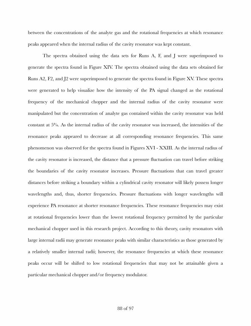
between the concentrations of the analyte gas and the rotational frequencies at which resonance

peaks appeared when the internal radius of the cavity resonator was kept constant.

The spectra obtained using the data sets for Runs A, F, and J were superimposed to

generate the spectra found in Figure XIV. The spectra obtained using the data sets obtained for

Runs A2, F2, and J2 were superimposed to generate the spectra found in Figure XV. These spectra

were generated to help visualize how the intensity of the PA signal changed as the rotational

frequency of the mechanical chopper and the internal radius of the cavity resonator were

manipulated but the concentration of analyte gas contained within the cavity resonator was held

constant at 5%. As the internal radius of the cavity resonator was increased, the intensities of the

resonance peaks appeared to decrease at all corresponding resonance frequencies. This same

phenomenon was observed for the spectra found in Figures XVI - XXIII. As the internal radius of

the cavity resonator is increased, the distance that a pressure fluctuation can travel before striking

the boundaries of the cavity resonator increases. Pressure fluctuations that can travel greater

distances before striking a boundary within a cylindrical cavity resonator will likely possess longer

wavelengths and, thus, shorter frequencies. Pressure fluctuations with longer wavelengths will

experience PA resonance at shorter resonance frequencies. These resonance frequencies may exist

at rotational frequencies lower than the lowest rotational frequency permitted by the particular

mechanical chopper used in this research project. According to this theory, cavity resonators with

large internal radii may generate resonance peaks with similar characteristics as those generated by

a relatively smaller internal radii; however, the resonance frequencies at which these resonance

peaks occur will be shifted to low rotational frequencies that may not be attainable given a

particular mechanical chopper and/or frequency modulator.

! of !88 97

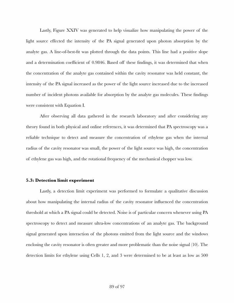
Lastly, Figure XXIV was generated to help visualize how manipulating the power of the

light source effected the intensity of the PA signal generated upon photon absorption by the

analyte gas. A line-of-best-fit was plotted through the data points. This line had a positive slope

and a determination coefficient of 0.9846. Based off these findings, it was determined that when

the concentration of the analyte gas contained within the cavity resonator was held constant, the

intensity of the PA signal increased as the power of the light source increased due to the increased

number of incident photons available for absorption by the analyte gas molecules. These findings

were consistent with Equation I.

After observing all data gathered in the research laboratory and after considering any

theory found in both physical and online references, it was determined that PA spectroscopy was a

reliable technique to detect and measure the concentration of ethylene gas when the internal

radius of the cavity resonator was small, the power of the light source was high, the concentration

of ethylene gas was high, and the rotational frequency of the mechanical chopper was low.

5.3: Detection limit experiment

Lastly, a detection limit experiment was performed to formulate a qualitative discussion

about how manipulating the internal radius of the cavity resonator influenced the concentration

threshold at which a PA signal could be detected. Noise is of particular concern whenever using PA

spectroscopy to detect and measure ultra-low concentrations of an analyte gas. The background

signal generated upon interaction of the photons emitted from the light source and the windows

enclosing the cavity resonator is often greater and more problematic than the noise signal (10). The

detection limits for ethylene using Cells 1, 2, and 3 were determined to be at least as low as 500

! of !89 97

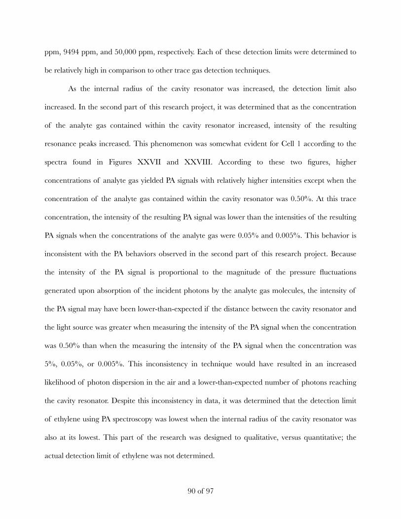
ppm, 9494 ppm, and 50,000 ppm, respectively. Each of these detection limits were determined to

be relatively high in comparison to other trace gas detection techniques.

As the internal radius of the cavity resonator was increased, the detection limit also

increased. In the second part of this research project, it was determined that as the concentration

of the analyte gas contained within the cavity resonator increased, intensity of the resulting

resonance peaks increased. This phenomenon was somewhat evident for Cell 1 according to the

spectra found in Figures XXVII and XXVIII. According to these two figures, higher

concentrations of analyte gas yielded PA signals with relatively higher intensities except when the

concentration of the analyte gas contained within the cavity resonator was 0.50%. At this trace

concentration, the intensity of the resulting PA signal was lower than the intensities of the resulting

PA signals when the concentrations of the analyte gas were 0.05% and 0.005%. This behavior is

inconsistent with the PA behaviors observed in the second part of this research project. Because

the intensity of the PA signal is proportional to the magnitude of the pressure fluctuations

generated upon absorption of the incident photons by the analyte gas molecules, the intensity of

the PA signal may have been lower-than-expected if the distance between the cavity resonator and

the light source was greater when measuring the intensity of the PA signal when the concentration

was 0.50% than when the measuring the intensity of the PA signal when the concentration was

5%, 0.05%, or 0.005%. This inconsistency in technique would have resulted in an increased

likelihood of photon dispersion in the air and a lower-than-expected number of photons reaching

the cavity resonator. Despite this inconsistency in data, it was determined that the detection limit

of ethylene using PA spectroscopy was lowest when the internal radius of the cavity resonator was

also at its lowest. This part of the research was designed to qualitative, versus quantitative; the

actual detection limit of ethylene was not determined.

! of !90 97

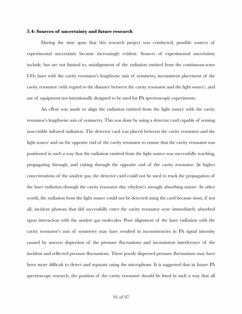
5.4: Sources of uncertainty and future research

During the time span that this research project was conducted, possible sources of

experimental uncertainty became increasingly evident. Sources of experimental uncertainty

include, but are not limited to, misalignment of the radiation emitted from the continuous-wave

CO2 laser with the cavity resonator’s lengthwise axis of symmetry, inconsistent placement of the

cavity resonator (with regard to the distance between the cavity resonator and the light source), and

use of equipment not intentionally designed to be used for PA spectroscopic experiments.

An effort was made to align the radiation emitted from the light source with the cavity

resonator’s lengthwise axis of symmetry. This was done by using a detector card capable of sensing

non-visible infrared radiation. The detector card was placed between the cavity resonator and the

light source and on the opposite end of the cavity resonator to ensure that the cavity resonator was

positioned in such a way that the radiation emitted from the light source was successfully reaching,

propagating through, and exiting through the opposite end of the cavity resonator. At higher

concentrations of the analyte gas, the detector card could not be used to track the propagation of

the laser radiation through the cavity resonator due ethylene’s strongly absorbing nature. In other

words, the radiation from the light source could not be detected using the card because most, if not

all, incident photons that did successfully enter the cavity resonator were immediately absorbed

upon interaction with the analyte gas molecules. Poor alignment of the laser radiation with the

cavity resonator’s axis of symmetry may have resulted in inconsistencies in PA signal intensity

caused by uneven dispersion of the pressure fluctuations and inconsistent interference of the

incident and reflected pressure fluctuations. These poorly dispersed pressure fluctuations may have

been more difficult to detect and separate using the microphone. It is suggested that in future PA

spectroscopy research, the position of the cavity resonator should be fixed in such a way that all

! of !91 97

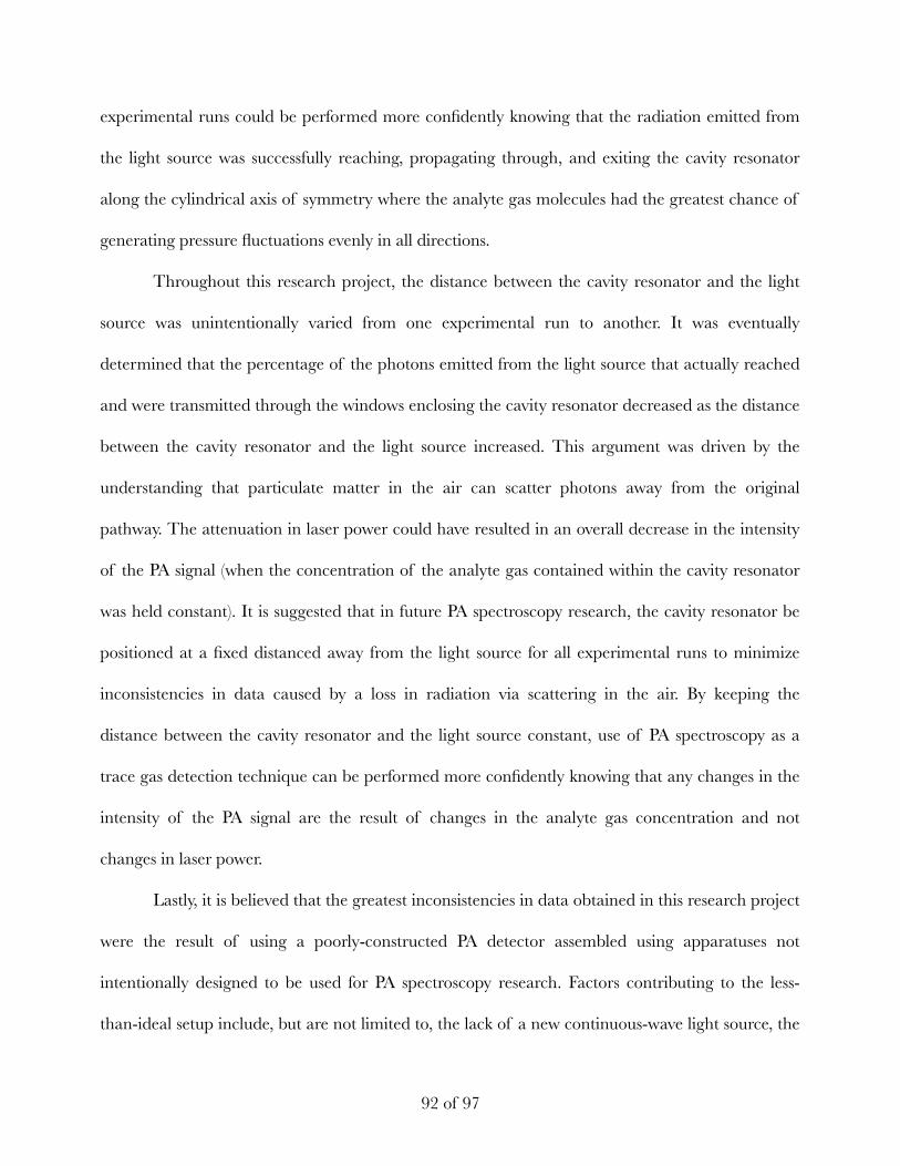
experimental runs could be performed more confidently knowing that the radiation emitted from

the light source was successfully reaching, propagating through, and exiting the cavity resonator

along the cylindrical axis of symmetry where the analyte gas molecules had the greatest chance of

generating pressure fluctuations evenly in all directions.

Throughout this research project, the distance between the cavity resonator and the light

source was unintentionally varied from one experimental run to another. It was eventually

determined that the percentage of the photons emitted from the light source that actually reached

and were transmitted through the windows enclosing the cavity resonator decreased as the distance

between the cavity resonator and the light source increased. This argument was driven by the

understanding that particulate matter in the air can scatter photons away from the original

pathway. The attenuation in laser power could have resulted in an overall decrease in the intensity

of the PA signal (when the concentration of the analyte gas contained within the cavity resonator

was held constant). It is suggested that in future PA spectroscopy research, the cavity resonator be

positioned at a fixed distanced away from the light source for all experimental runs to minimize

inconsistencies in data caused by a loss in radiation via scattering in the air. By keeping the

distance between the cavity resonator and the light source constant, use of PA spectroscopy as a

trace gas detection technique can be performed more confidently knowing that any changes in the

intensity of the PA signal are the result of changes in the analyte gas concentration and not

changes in laser power.

Lastly, it is believed that the greatest inconsistencies in data obtained in this research project

were the result of using a poorly-constructed PA detector assembled using apparatuses not

intentionally designed to be used for PA spectroscopy research. Factors contributing to the less-

than-ideal setup include, but are not limited to, the lack of a new continuous-wave light source, the

! of !92 97

lack of a more uniformly-shaped set of cylindrical cavity resonators, and the lack of system

capable of producing vacuum-like or near-vacuum-like conditions within the cavity resonator. It

was believed that repeat use of the particular light source and controller used in this research

project for other experiments in the past may have negatively affected its ability to emit consistent

and high-power radiation. Upon detailed analyses of the data obtained in this research project, it

was determined that several of the inconsistencies observed may likely the result of using

cylindrical cavity resonators that were not uniformly-shaped. For experiments involving the

manipulation of the internal radii, any changes in PA signal intensity observed should primarily

have been the result of variations in internal radii and not the result of variations in the overall

shape of the cavity resonator, itself. In this research project, the three cavity resonators were

constructed using apparatuses that were not specifically designed for PA spectroscopic experiments.

The effect that the three cavity resonator’s variation in shape had on the PA signal became

increasingly evident for Cells 2 and 3. Lastly, it was also believed that inconsistencies in data

obtained were the result of using a non-vacuum or non-near-vacuum-like apparatus. For each

experimental run performed in this research project, the cavity resonator was thoroughly rinsed

and filled with the inert buffer gas nitrogen. The cavity resonator was then filled with pre-

determined volumes of ethylene gas to achieve specific concentrations of analyte gas contained

within the cavity resonator. In theory, it is impossible for a closed system to contain any gas solution

whose volume is effectively greater than the volume of the closed system, itself. In this research

project, it was assumed that the cavity resonator used was not entirely enclosed and that leakage

could occur if need be. In a vacuum system, the exact pressure within the cavity resonator could

have been regulated. Rather than assuming that the total pressure within the cavity resonator was

1 atm, the exact total pressure could have been determined and used to further discuss the PA

! of !93 97

behavior of ethylene. It is suggested that in future PA spectroscopy research, a new continuous-

wave light source, more uniformly-cylindrical cavity resonators, and a system capable of producing

vacuum-like or near-vaccuum-like conditions be used to help minimize inconsistencies in data

caused by less-than-ideal PA detectors.

Statement of Results

This research project was performed to determine which experimental conditions best

enabled precise and accurate measurements of ethylene using PA spectroscopy as a form of trace

gas detection. It was determined that PA spectroscopy technique was most reliable when the

internal radius of the cavity resonator was small, the power of the light source was high, the

concentration of ethylene gas was high, and the rotational frequency of the mechanical chopper

was low. These experimental conditions should be considered by manufacturers when devising

highly-sensitive, low-cost, portable systems for the measurements of ethylene gas both inside and

outside the laboratory.

! of !94 97

Acknowledgements

Dr. Han J. Park, Ph.D., Thesis Director

Dr. Manuel F. Santiago, Ph.D., Department Examiner

Dr. Titus V. Albu, Ph.D., Department Examiner

Grote Fund, Department of Chemistry and Physics, UTC

Innovations in Honors Program, Honors College, UTC

Chapel Cowden, Health and Science Instruction Librarian, Library, UTC

! of !95 97

References

1. McNaghten, E.D.; Parkes, A.M.; Griffiths, B.C.; Whitehouse, A.I.; Palanco, S. Detection of

Trace Concentrations of Helium and Argon Gas in Mixtures by Laser-Induced

Breakdown Spectroscopy [Online]. Spectrochimica Acta. 2009, 1111-1118.

2. Harren, F. J. M.; Cotti, G.; Oomens, J.; Hekkert, S. L. Photoacoustic Spectroscopy in Trace Gas

Monitoring. Encyclopedia of Analytical Chemistry; John Wiley & Sons: Chichester, 2012; pp.

2203-2226.

3. Gondal, M. A.; Dastageer, A.; Yamani, Z. H. Laser-Induced Photoacoustic Detection of Ozone

at 266 nm Using Resonant Cells of Different Configuration [Online]. J. Environ. Sci.

Heal. A. 2009, 44, 1457-1464.

4. Janssen, S.; Schmitt, K.; Blanke, M.; Bauersfeld, M. L.; Wöllenstein, J.; Lang, W.; Ethylene

Detection in Fruit Supply Chains [Online]. Philos. T. Roy. Soc. A. 2014, 372, 1-21.

5. Lutrell, W. E. Ethylene [Online]. J. Chem. Health Safety. 2016, 23, 43-45.

6. Bleeker, A. Ethylene [Online]. Curr. Biol. 2011, 11, 952.

7. Ritenour, M. A.; Brecht, J. K. Ethylene Treatments for Ripening & Degreening, 2013.

8. Ethylene; MSDS No. 001022 [Online]; Airgas USA: Radnor, PA, Feb 6, 2004. https://

terpconnect.umd.edu/~choi/MSDS/Airgas/ETHYLENE.pdf (accessed Mar 5, 2017).

9. Esler, M.B.; Griffith, D.W.T.; Wilson, S.R.; Steele, L.P. Precision Trace Gas Analysis by FT-IR

Spectroscopy. 1. Simultaneous Analysis of CO2, CH4, N2O, and CO in Air [Online].

Anal. Chem. 2000, 72, 206-215.

10.Miklós, A.; Hess, P.; Modulated and Pulsed Photoacoustics in Trace Gas Analysis. Anal. Chem.

2000, 72, 30-37.

! of !96 97

11.Murphy, W. S.; Park, H. J. Detecting Photoacoustic Signals of Sulfur Hexafluoride at Varying

Microphone Positions [Online]. Open J. Phys. Chem. 2016, 6, 49-53.

12.Park, H. J.; Murphy, W. S. A Study of the Photoacoustic Effect in SF6 at High Concentrations

and at Trace Detects in N2 [Online]. Journal of Undergraduate Chemistry Research. 2015, 14,

90-92.

13.Park, H. J. Photoacoustic Effect and Sonoluminescence Generated by Laser Initiated

Exothermic Chemical Reactions. Ph.D. Thesis, Brown University, Providence, RI, 2011.

14.Rosencwaig, A. Photoacoustic Spectroscopy of Solids [Online]. Phys. Today 1975, 28,

23-30.Miklós, A.; Hess, P. Application of Acoustic Resonators in Photoacoustic Trace

Gas Analysis and Metrology [Online]. Rev. Sci. Instrum. 2001, 72, 1937-1955.

15.Ball, D. W. Photoacoustic Spectroscopy [Online]. Spectroscopy 2006, 21, 14-16.

16.Photoacoustic Spectroscopy, Theory. Encyclopedia of Spectroscopy and Spectrometry; Academic Press:

San Diego, 1999; pp. 1815-1822.

17.Schmid, T. Photoacoustic Spectroscopy for Process Analysis [Online]. Anal. Bioanal. Chem. 2006,

384, 1071-1086.

18.Nitrogen; MSDS No. 00104 [Online]; Airgas USA: Radnor, PA, May 26, 2016. https://

www.airgas.com/msds/001040.pdf (accessed Mar 5, 2017).

19.Kaneko, F.; Monjushiro, H.; Nishiyama, M.; Kasai, T. Photoacoustic Experimental System to

Confirm Infrared Absorption Due to Greenhouse Gases [Online]. J. Chem. Educ. 2010,

87, 204-206.

! of !97 97