A STUDY OF MACRO-CELL AND MICRO-CELL CORROSION OF STEEL IN CONCRETE

(Translation from Proceedings of JSCE, No.732/V-59, May 2003)

Tatsuo KAWAHIGASHI Koichi KOBAYASHI Toyoaki MIYAGAWA The use of non-destructive methods to evaluate the corrosion of reinforcing steel in concrete is one crucial tool for the maintenance of concrete structure. However, such methods are still in the examination stage, both with respect to methodology (type of non-destructive methods and implementation) and evaluation of measured values. Still, there is expectation that evaluation methods will soon be established. In this investigation, non-destructive methods such as measurements of half-cell potential, polarization resistance (AC impedance), and electric current are tested in a model experiment using different sized steel plates, leading to an understanding of changes in electrochemical response of the reinforcing steel. Macro-cell corrosion and micro-cell corrosion are then calculated from the experiment results using numerical methods. This study shows that it is possible to separate macro-cell corrosion from micro-cell corrosion, and that steel reinforcement corrosion can be estimated.

Keywords: chloride, steel corrosion, electrochemical method, half-cell potential, polarization resistance, concrete resistance, electric current, macro-cell, micro-cell, numerical analysis Tatsuo Kawahigashi is an assistant professor in the Institute for Science and Technology, Kinki University, Higashi-Osaka, Japan. He obtained his Dr. Eng. from Kyoto University in 2002. His research interests relate to the corrosion/deterioration mechanism and the estimation of durability of concrete structures. He is a member of JSMS, JCI, and JSCE. Koich Kobayashi is an assistant professor in the Department of Civil Engineering, Chubu University, Kasugai, Japan. He obtained his Dr. Eng. from Kyoto University in 1999. His research interests relate to chloride induced corrosion of reinforcing steel in concrete. He is a member of JSMS, JCI, and JSCE. Toyoaki Miyagawa is a professor in the Department of Civil Engineering, Kyoto University, Kyoto, Japan. He obtained his Dr. Eng. from Kyoto University in 1985. He is the author of a number of papers dealing with the durability, maintenance, and repair of reinforced concrete structures. He is a member of ACI, RILEM, fib, JSMS, JCI, and JSCE.

65

1. INTRODUCTION Non-destructive methods currently available for evaluating reinforcing steel corrosion in concrete include half-cell potential and polarization resistance. The half-cell potential method is most widely used in assessing corrosion because measurements are easy and measured values correlate well with corrosion conditions. On the other hand, the polarization resistance method yields an estimate of the rate of reinforcing steel corrosion, leading to predictions of future corrosion-related deterioration. However, such methods are still in the examination stage, both with respect to methodology and evaluation of measured values. It is expected that evaluation methods based on these methodologies will soon be established. [1] Steel corrosion in concrete is understood to occur through both macro-cell corrosion and micro-cell corrosion, and the interaction of the two is seen as advancing corrosion. At present, it remains difficult to distinguish between the two forms of corrosion and to estimate their progress using these non-destructive methods. An important task, therefore, is to establish evaluating of steel corrosion by a non-destructive methodology after understanding this mechanism of steel corrosion. Recently, various non-destructive and numerical methods have been used and many cases of steel corrosion are examined. For example, methods of evaluating corrosion through various numerical methods and evaluating macro-cell corrosion and micro-cell corrosion using measurements have been proposed [2][3][4]. However, there are few reports on estimating of corrosion loss with distinguishing the macro-cell and micro-cell corrosion and with resembling a actuality phenomenon. In this study, for distinguishing between macro-cell and micro-cell corrosion, electrochemical non-destructive methods are used to measure steel plate corrosion induced by chloride ions. There are two main aims for the investigation: (1) comparison of macro-cell corrosion analysis using half-cell potential, concrete resistance and polarization resistance (2) estimation of corrosion loss and relation of macro-cell corrosion between analysis, electric-current and polarization resistance 2. EXPERIMENTAL OUTLINE 2.1 Materials and mix proportion of concrete The materials used are shown in Table 1, and the concrete mix proportion, air volume, slump, and 28-d compressive strength obtained in measurements are shown in Table 2. 2.2 Test specimens Details of the concrete and steel plate are given in Fig. 1(a). Two types of test specimen were produced, for the following purposes: (1) Specimens with a single long steel plate for the purpose of examining macro-cell corrosion (L specimens) (2) Specimens with a short steel plate for the purpose of examining macro-cell (connected together in series with leads wire) and micro-cell (disconnected together) corrosion (S specimens) All steel plates were of the same material, thickness and width, and all surfaces except face for the purpose of

66

corroding were coated with epoxy. In the Series 1 (L) experiments, the steel plate was 1.6 mm thick, 15 mm wide, and 1930 mm long. All faces except 15x1810 mm area of top surface for the purpose of corroding were coated with epoxy. When casting the concrete, a polypropylene cylinder of 10 mm diameter was inserted to a depth of 5 mm to the exposure surface at one ends of steel plate. It was removed after the concrete had set. The cavity left by this cylinder formed the cell for supplying salt water. In the Series 2 (S) experiments, all steel plates except both ends plates were 1.6 mm thick, 15 mm wide, and 98 mm long, and each specimen had fixtures for lead wire at both edges. The steel plates of both ends were respectively 168 mm long (salt water supplying cell side) and 158 mm long (other side). All surfaces except exposure surface for the purpose of corroding were coated with epoxy (as with the L specimens), and the total length of the exposure surface was 1720 mm. A polypropylene cylinder was used to form the saltwater cell, with the L specimens. Concrete was cast on to the steel plate, which was put onto insulated adhesive sealing tape overlying the form. No concrete cracking occurred in removing the forms nor during the examination period, though the possibility of cracking was considered. 2.3 Curing and environmental conditions After 48 hours from casting, specimens were cured in water for 14 days and then in air indoors for fixedness period. The steel plate was started to be corroded after the dry-curing in the period. To limit the corrosion position and to ensure penetration into the concrete specimen as in actual salt diffusion, salt water was supplied regularly to the cell. The salt water consisted of 3 mass percent NaCl and was supplied at a rate of about 5-6 cc per day to ensure that the cell was always filled. It was supplied through a silicon tube of diameter 1 mm from a saltwater bottle. 2.4 Measurements Measurements consisted of electrochemical measurements and a steel mass loss measurement (after removing the steel plate from the concrete). a) Measurement conditions Electrochemical measurements consisted of half-cell potential and polarization/concrete resistance (by the AC

B-type blast-furnace slag cement, slag wt.: 40%, specific gravity: 3.05g/cm3，Blaine's specific surface area：3980cm2/g

　SiO2: 25.4, Al2O3: 8.3, Fe2O3: 2.3, CaO: 55.9, MgO: 3.6, SO3: 1.9 　Na2O: 0.25, K2O: 0.43, TiO2: 0.55, P2O5: 0.09, MnO: 0.16, ig.loss: 0.7

Content (%) 　 C3S: 31, C2S: 13, C3A: 5, C4AF: 5Fine Agg. 　River sand, specific gravity: 2.55g/cm3, F.M.: 2.74, water absorption: 2.19 (%)Coarse Agg. 　Crushed stone, specific gravity: 2.67g/cm3, F.M.: 6.29, water absorption: 0.95, max. size: 15mm

　Steel plate: rolled steel for general structures, SS41(SS400); quality: acid processing; thickness: 1.6mm

Table 1 Materials

Cement　Chemical

composition(%)

Aggregate

Reinforcing steel

W C S G AE agent Compressive Bending0.5 46.8 185 370 755 899 ― 2.0 8.5 33.9 5.6

Table 2　Mix proportion and measured values of concrete

W/C Sand volumeratio s/a (%)

Unit weight （kg/m3） Measured air

volume（％）

Measuredslump（cm）

Meas. strength 28-d（N/mm2）

67

Fig. 1 Dimensions of specimen, measurement outline, and position of measurement points impedance method), as well as current flow between steel plates in the S specimens (Fig.1 (a)). These measurements were done after wetting concrete surface. AC impedance measurements were made at a voltage of +10 mV/-10 mV and at a frequency of 10-Hz/0.01-Hz. The reference electrode for the half-cell potential, polarization resistance, and concrete resistance measurements was used with a saturated silver chloride electrode. For the counter-pole in AC impedance measurements, a double type was used (these diameter were 40 mm and 106 mm). [5]

AC impedance Half-cell potential　　　No.1→ reference electrode, counter pole reference electrode → No.21-37 Steel plate width

50mm 15mm

Steel plate exposure surface (L: 1810mm, S: 1720mm) Resin coat (60mm) Resin coated length (60mm)

　1930mm

　　　Resin coat + Friction tape Lead (Connection)Exposure surface

　　 （Resin coat）AC impedance corrosion monitor(Polarization/concrete resistance) 　To steel end

　　 98mm (Exposure surface: 95mm) Distance among plate: 2mm Outline of short steel plate S Potential reference electrode

AC impedance reference electrode, counter pole (Ag/AgCl) Steel thickness (Ag/AgCl, stainless double counter pole)

1.6mm 20 mm

Concrete dimensions　( width×length×thickness　50×1850×20 mm )Steel dimensions　( width×length×thickness　L: 15×[1930]×1.6mm, S: 15×[168＋98×16＋158=1894]×1.6mm )

Top　　　Concrete width

Electrometer(Half-cell potential)

Concrete thickness

Side

(a)　Dimensions of steel and concrete, and measurement outline

Salt water cell（φ13×15mm-depth）

Distance from cell(mm) 0 10 60 250 500 750 1000 1250 1500 1810 Meas.points

　 ●◎ □ 37

18resistance

　 ●◎ □ 21

18resistance

○ 　 ○ ○　 ○ ○ ○　 ○ ○　 ○ ○　 ○ 17among steel plate

　 ●◎ □ 21

18resistance

Note 1)　L: Long steel plate, S-MA: Short steel plate (lead connected), S-mi: Short steel plate (lead disconnected)

Note 2) ● Potential in salt water cell，　◎: Potential invicinity salt water cell，　□: Potential of steel exposure surface end

L　 Potential ○ ○ ○ ○○ ○ ○ ○ ○○ ○ ○ ○ ○○ ○ ○ ○ ○○ ○○ ○○ ○○ ○○ ○○ ○○ ○○

L　 Polarization/concrete ○ ○ ○ ○ ○ ○ ○ ○ ○ ○ ○ ○ ○ ○ ○ ○ ○ ○

S-MA　Potential ○ ○ ○ ○ ○ ○ ○ ○ ○ ○ ○ ○ ○ ○ ○ ○ ○ ○

S-MA　Polarization/concrete ○ ○ ○ ○ ○ ○ ○ ○ ○ ○ ○ ○ ○ ○ ○ ○ ○ ○

S-MA　Electric current ○　　○　　 ○ ○　　○　　 ○

S-mi　 Potential ○ ○ ○ ○ ○ ○ ○ ○ ○ ○ ○ ○ ○ ○ ○ ○ ○ ○

S-mi　 Polarization/concrete ○ ○ ○ ○ ○ ○ ○ ○ ○ ○ ○ ○ ○ ○ ○ ○ ○ ○

(b)　Position of measurement points

68

Mass loss due to steel corrosion was measured by immersing the steel plate in citric 2-ammonium solution (10% concentration) for 24 hours, and was obtained from the mass difference from before immersion and after immersion. Therefore, to extract the influence over the steel mass loss measurement was done as follows; three same kind steel plates with coating were immersed in same acid solution, and the mass of the fine aggregate peeled from steel was obtained by filtering. b) Measurement points The number of electrochemical measurement points and their position is shown for each specimen in Fig.1 (b). In the case of L specimens, the half-cell potential was measured at 37 points at 50-mm intervals, while polarization resistance and concrete resistance were measured at 18 points at 100-mm intervals. In the case of S specimens, the half-cell potential was measured at 21 points, including the center point of each steel plate, the vicinity of the salt water cell, and the leftmost end of the steel plate. Polarization resistance and concrete resistance were measured at 18 points, consisting of the same points as half-cell potential except for salt water cell inner and rightmost/leftmost ends. In the case of S specimens, each measurement was taken under two conditions: with the lead wires of short plates connecting and with the leads temporarily disconnected. An influence on the measurement was just before disconnecting/connecting the leads. Therefore, the half-cell potential was measured first and each measurement was taken after confirming that the potential had stabilized. As for the current flow in the S specimens, the current between steel plates was measured while the leads between them were connected. 3. RESULTS AND DISCUSSION 3.1 Changes in measured value a) Changes in average potential and potential distribution The average potential in L specimens and S specimens before and after supplying salt water is shown in Fig. 2. The average values while curing and before supplying salt water are similar. One specimen each from among the L specimens and the S specimens was chosen for the addition of salt water, and these were kept regularly supplied with salt water in the cell. These specimens are denoted, respectively, by "L1" and "S1". The average half-cell potential fell (shown rise in Figure) to negative (base) value rapidly during dry curing and supplying salt water in both cases, as shown in Fig. 2 (b): at about 800 hours for L1 and about 1300 hours for S1. As shown by the black arrow in Fig. 2 (b), the base period changed remarkably about 300 hours from the starting base both in L1 and S1, and thereafter the gradients became more gentle. The time at which the base beginning occurs is different because the depth of mortar below the salt water to reach the steel plate was different, so the time taken for the salt water to reach the steel plate would differ. As a result, the beginning of corrosion was about 800 hours after supplying salt water in L1 and about 1300 hours after supplying salt water in S1. In applying numerical analysis to investigate macro-cell corrosion, the measured value from the time at which the gradient of the change in base became flatter (about 1100 hours for L1 and 1600 hours for S1) was adopted. The potential distribution of each point on the specimen before and after the sudden change in average potential after supplying salt water to the cell is shown in Fig. 3. As for the potential of L1 (at 335 hours) and S1 (at 336 hours with the leads connected), there is no significant difference among measurement points. However, after the potential near the salt water cell changed into the base, the values of both L1 and S1 became the base in the vicinity of the salt water cell, while it became noble (rising to positive value) with distance from this point.

69

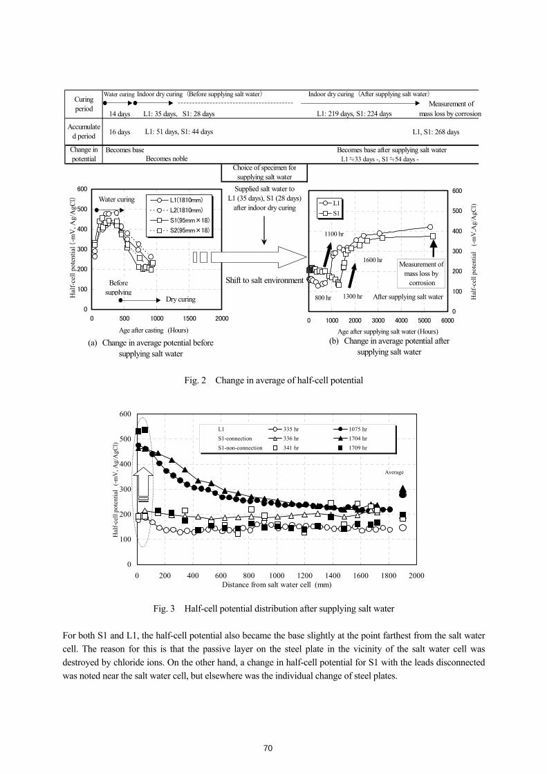
Fig. 2 Change in average of half-cell potential

Fig. 3 Half-cell potential distribution after supplying salt water For both S1 and L1, the half-cell potential also became the base slightly at the point farthest from the salt water cell. The reason for this is that the passive layer on the steel plate in the vicinity of the salt water cell was destroyed by chloride ions. On the other hand, a change in half-cell potential for S1 with the leads disconnected was noted near the salt water cell, but elsewhere was the individual change of steel plates.

Water curing Indoor dry curing（Before supplying salt water） Indoor dry curing（After supplying salt water）

14 days mass loss by corrosion

16 days L1, S1: 268 days

Becomes base Becomes base after supplying salt waterL1≒33 days -, S1≒54 days -

Curingperiod

Measurement of L1: 35 days，S1: 28 days L1: 219 days, S1: 224 days

Accumulated period L1: 51 days, S1: 44 days

Change inpotential 　 Becomes noble

Supplied salt water toL1 (35 days), S1 (28 days)

after indoor dry curing

Shift to salt environment

Choice of specimen forsupplying salt water

(b)　Change in average potential aftersupplying salt water

0

100

200

300

400

500

600

0 1000 2000 3000 4000 5000 6000

Age after supplying salt water (Hours)

Hal

f-ce

ll po

tent

ial 　

(-m

V,A

g/A

gCl)L1

S1

800 hr 1300 hr

1100 hr

1600 hr Measurement ofmass loss by corrosion

After supplying salt water

(a)　Change in average potential beforesupplying salt water

0

100

200

300

400

500

600

0 500 1000 1500 2000

Age after casting　(Hours)

Hal

f-ce

ll po

tent

ial （

-mV

, Ag/

AgC

l ） L1(1810mm)

L2(1810mm)

S1(95mm×18)

S2(95mm×18)

Water curing

Beforesupplying

Dry curing

0

100

200

300

400

500

600

0 200 400 600 800 1000 1200 1400 1600 1800 2000Distance from salt water cell (mm)

Hal

f-ce

ll po

tent

ial 　

(-m

V, A

g/A

gCl)

L1 335 hr 1075 hrS1-connection 336 hr 1704 hrS1-non-connection 341 hr 1709 hr

Average

70

b) Distribution of polarization/concrete resistance The distributions of true polarization resistance and apparent concrete resistance for specimens L1 and S1 are shown respectively in Fig. 4 (a) and (b). Concrete resistance is the apparent value, but this will form the basis of the analysis in the following paragraph. The polarization resistance and concrete resistance near the salt water cell decreased once the average potential became notably base, and these phenomena show a corrosion tendency like the results of half-cell potential.[6] After 1,075 hours in the case of L1, the polarization/concrete resistance at points far from 1200 mm from the salt water cell are larger than at points nearer than 1200 mm. Under leads disconnected after supplying saltwater, the polarization/concrete resistance in the case of specimen S1 at 1,709 hours are larger than at 341 hours except the neighborhood of the cell. Looking at the mass loss of the steel plate due to corrosion, adhesion between the steel plate and the concrete was not lost in specimens L1 and S1. Consequently, such a phenomenon (for polarization/concrete resistance) occurred because of formation of a passive layer, and because of drying between concrete and steel plate. The variations in concrete resistance between L1 and S1 result from environmental differences at measurement period and from varying moisture condition of the concrete.

(a) Polarization resistance distribution (b) Concrete resistance distribution

Fig. 4 Polarization resistance and concrete resistance distribution after supplying salt water 3.2 Analysis using measurement results Corrosion cases using the measurement and analysis results are shown in Table 3. Corrosion quantity (W ) of the steel plate by calculating from the measurement and analysis was estimated by the following formula:

W (g/cm2) =ac

I dtcorr∫ =ac K R dtp( / )1∫ (1)

where, Icorr: corrosion current density (A/cm2); K: proportional constant (V); Rp: polarization resistance (Ω･

cm2); a: value of at. wt. of iron divided by valency 2 (27.9g); and c: the Faraday constant (96,500C) The corrosion cases examine using specimens L1 and S1, as shown in Table 3, are classified as follows: L1: Corrosion estimated from macro-cell analysis (L1-MA: 1) and corrosion estimated from polarization resistance (L1-MA: 2)

1

10

100

1000

10000

0 200 400 600 800 1000 1200 1400 1600 1800 2000

Act

ual p

olar

izat

ion

resi

stan

ce　(k

Ω･ c

m2)

L1 335 hr 1075 hrS1-connection 336 hr 1704 hrS1-non-connection 341 hr 1709 hr

Average

Distance from salt water cell (mm)

0

5

10

15

0 200 400 600 800 1000 1200 1400 1600 1800 2000

Distance from salt water cell　（mm）

Con

cret

e re

sist

ance

　(k

Ω)

L1 335 hr 1075 hrS1-connection 336 hr 1704 hrS1-non-connection 341 hr 1709 hr

Average

71

Table 3 Corrosion cases for specimens L1 and S1

S1: Corrosion estimated from macro-cell analysis with leads connecting the steel plates (S1-MA: 3), corrosion estimated from the polarization resistance of each point (S1-MA-mi: 4), and micro-cell corrosion estimated from the polarization resistance the steel plates are disconnected (S1-mi: 5) Generally, examinations of macro-cell corrosion involve analysis 1 for L1. Examination 2 estimates the macro-cell corrosion and overall micro-cell corrosion. As shown in Fig. 3 and Fig. 4, however, it is considered that corroded parts influence the change toward base potential in non-corroded area. Therefore, it is difficult to obtain a strict value only of the corroded part because nearby non-corroded areas are assumed to be corroded part in some cases. On the other hand, in the case of S1, it is possible to examine 2 from a comparison of 4 and 5, and moreover it is possible to compare it with 1. Examining the case of S1 is important for evaluating macro-cell corrosion and micro-cell corrosion individually and for examining a general case like L1. It was supposed that macro-cell corrosion had not occurred in each steel plate when S1 was separated. The numerical analysis of macro-cell corrosion is described in the following paragraph. a) Analysis of macro-cell corrosion Generally, the distribution of two-dimensional potential (u) in concrete determined using Laplace's equation, as (2) below.

∂∂

∂∂

2

2

2

2 0ux

uy+ = (2)

The equation can be solved by calculus of finite difference [7] or a fininte-element method [8]. The following conditions were used to analyze Laplace's equation and the finite difference method was applied. (a) An approximate quantic curve was fitted to the measured potential at the fixed intervals (L1: 50 mm; S1: 95 mm), and the potential obtained for every 2.5 mm interval for analysis using the finite difference method.

(b) It was supposed that the concrete surface potential was the steel plate surface potential in (a) because the thickness of concrete was thin as 20 mm [3]. As the boundary condition, it is supposed that the concrete surface and both ends had a potential equal to the neighbor potential at the closest internal point. The number of axial analysis node was 725 (L1) and 689 (S1), so the total node count in the analysis was (steel plate axial direction) x 8 (the direction of concrete depth) = 5,800 (L1) and 5,512 (S1). Calculations were iterated until the difference between each node potential and the previous potential was equal or less than 0.0001 mV. (c) The inward/outward flow of electric current and the corrosion current density at the steel plate surface were obtained from the potential distribution in (b), the concrete resistance as resistivity [9], and the polarization resistance of each measurement point.

An outline of the analysis is given in Fig. 5. Nodes were arranged at the 2.5-mm intervals and resistors were set up among nodes. For example, in the vertical direction, it was supposed that 16 lines of eight series resistors made up the axial section of 40 mm in a section 20 mm in length. Resistance between pairs of nodes was calculated from the serial and parallel relations for resistance. The polarization resistance was assumed to be the resistance of the polarization layer, which is marked in Fig. 5, dividing the true polarization resistance by an area measuring 15 mm in width of 2.5-mm sections of the steel plate.

L1: Large steel plate (Exposure surface:15×1810 mm)

S1: Short steel plate (Exposure surface: 15×95 mm×18+10 mm)

Macro-cell corrosion of continuous steel plate L1-MA S1-MA Corrosion of continuous steel plate L1- MA-mi S1- MA-mi Micro-cell corrosion of separated steel plate ―――――――― S1- mi

72

Fig. 5 Analysis concept for half-cell potential distribution and current

73

b) Distribution of potential and current by macro-cell analysis The steel plate surface potential, which was obtained as an approximate quantic curve fitting the potential distribution after changing toward the base potential shown in Fig.3, is shown in Fig.6. The potential distribution for macro-cell corrosion analysis was obtained from regressing the approximate quantic curve to the points of measurement and non-measurement as described on (a) in paragraph a). Various formula were used for the regression curve, and the correlation of the 4th quantic was the highest with a coefficient of correlation "R2" of about 0.99. The measured potential at 10 mm intervals was compared with the value from the approximate expression, but there were no problems in the regression curve. The current distribution on the steel plate surface, as obtained in the analysis, is shown in Fig. 7. The inset figure is a magnification of the transverse direction in the vicinity of the salt cell of L1 and S1; it can be seen that the current calculated from the potential and concrete resistance is bigger than that when polarization resistance is considered. However, this difference was on the appearance and no conspicuous difference was found by integrated value which is equivalent to the anode current in the paragraphs that follow. From these results, it is considered that the difference in current between the potential/concrete-resistance and the potential /concrete-resistance/polarization-resistance calculations was not large, and that there was almost no difference in the analysis of corrosion current and macro-cell corrosion quantity.

Fig. 6 Half-cell potential distribution and application of quantic curve

Fig. 7 Vertical component of current for certain cases

L1 : E = -0.000000000000447L 4 - 0.0000000748958L 3

+ 0.0003179611L 2 - 0.4721919L + 480.393R2 = 0.9943

S1 : E = -0.0000000000507L 4 + 0.0000001722037L 3

- 0.00006114318L 2 - 0.288240L + 475.730R2 = 0.9894

0

100

200

300

400

500

600

0 200 400 600 800 1000 1200 1400 1600 1800 2000

Distance from salt water cell　L (mm)

Hal

f-ce

ll ot

entia

l 　E

　(-

mV

, Ag/

AgC

l)

-0 .02

0

0 .02

0 .04

0 .06

0 .08

0 .1

0 500 1000 1500 2000

D istance from sa lt w ater ce ll (m m )

Cur

rent　

(μA

)

S 1-1704 h r

Pot.+C on . res .

Pot.+C on . res .+Po l. res .

L1-1075 h r

Pot.+C on . res .

Pot.+C on . res .+Po l. res .

-0 .02

0

0 .02

0 .04

0 .06

0 .08

0 .1

0 20 40 60 80 100 120

D istance from sa lt w ate r ce ll　 (m m )

Ele

ctric

cur

rent

　（μ

A）

S 1-1704 h r

Pot.+C on . res .

Pot.+C on . res .+Po l. re s .

L1-1075 h r

Pot.+C on . res .

Pot.+C on . res .+Po l. re s .

74

c) Measured and estimated current with leads S1 connected (S1-MA) To allow comparison with analytical values, the current between steel plates was measured with a zero-resistance ammeter and the current in each steel plate obtained. These currents are shown in Fig. 8 (a), and each steel plate current, which is obtained from the difference of the current between steel plates, except for the plate containing the salt water cell are shown in Fig. 8 (b). The current was measured at the same time as measuring potential, polarization resistance, and concrete resistance. The concrete was not under dry-cured condition due to be measured and was under temporarily moist condition. If it is supposed that the current in each steel plate is as shown in Fig. 8 (b), it can be divided into anode and cathode currents. It is then possible to show the flow of current as in Fig. 9, from the relation between current distribution as shown in Fig. 7, and each calculated steel plate current. However, this figure does not mean the direction and start/end of the arrow corresponding to the direction and size of the total current because figure is an outline of the current flow.

Fig. 8 Measured current between steel plates and calculated current in steel plate

Fig. 9 Macro-cell current outline of model

(a) Measured current between steel plates

y = 2E-12x4 - 1E-08x3 + 2E-05x2 - 0.0239x + 9.7135R2 = 0.997

y = -4E-12x4 + 1E-08x3 + 4E-06x2 - 0.0301x + 22.411R2 = 0.9981

0

5

10

15

20

25

0 200 400 600 800 1000 1200 1400 1600 1800

Distance from salt water cell to center of plate (mm)

Cur

rent

bet

wee

n st

eel p

late

(µA

)

Period (hr)16081704185122082520

(b)　Current in steel plate from results of (a)

0

1

2

3

4

0 200 400 600 800 1000 1200 1400 1600 1800

Distance from salt water cell to center of plate (mm)

Cur

rent

in st

eel p

late

(µA

)Period (hr)

1608

1704

1851

2208

2520

Concrete

Salt water cellResin coated area

Resin coated area

Sc S1 S2 Sn Sn+1 S16 S17

Arrow : Outline of current in/out flow, 　Sc : Steel plate with cell,　S1 - S17 : Each plate

CC = (CB(C-1)-CB(1-2))+(CB(1-2)-CB(2-3))+…+(CB(15-16)-CB(16-17))+C17

= C1+C2+…+Cn+Cn+1+…+C16+C17=CB(C-1)-CB(16-17)+C17

Cc : Current in steel plate with cell ,　CB(C-1) : Current between steel plates with cell Sc and steel plate S1,

CB(n-(n+1)) : Current between No. (n) and No. (n+1) , Cn : Current in No. (n), n : 1 - 16

75

Fig. 10 Distribution of current supposing anode steel plate (with cell) and cathode steel plate (without cell)

Fig. 11 Current under moist/dry conditions (case of S1) From these relations, the current distribution is assuming that each steel current (C1-C17), as shown in Fig. 8 (b), is a cathode current and that the total current is the anode current (Cc) flowing from Sc as shown in Fig. 10. This is because Fig. 7 shows the distribution of current for each node on the 2.5-mm grid, whereas Fig. 10 shows the current for each steel plate. As already noted, these results were obtained with the specimen under moist conditions. On the other hand, it was considered important to grasp the current under dry conditions, as these are the conditions normally prevailing. This is because the difference, which is seemed to occur to the measured current under moist and dry condition, would have an affect on the analysis result. Therefore, the current measured under moist conditions (just after each measurement) was compared with that obtained under dry conditions (just before each measurement). The distribution of current between the steel plates and the steel plate current under the moist/dry condition after 3,192 hours of salt water supply is shown in Fig. 11 (a), and the change in anode current between moist and dry conditions is shown in Fig. 11 (b). Each current between steel plates under dry condition is estimating from a ratio under dry-moist condition.

-5

0

5

10

15

20

25

0 200 400 600 800 1000 1200 1400 1600 1800 2000

Distance from salt water cell to center of each steel plate (mm)

Elec

tric

curr

ent o

f eac

h pl

ate(

µA) Period (hr)

16081704185122082520

Anode current by totalcathode current frommeasured current betweensteel plates(under moist conditions)

(b) Change in anode current

0

5

10

15

20

25

30

0 500 1000 1500 2000 2500 3000 3500

Period (hr, after supplying salt water)

Tota

l cur

rent

(µA

: eq

uiva

lent

to a

node

cur

rent

） Under moist conditionsUnder dry conditions

(a) Measured value of current between steel plates and current in steel plate(3,190 hrs after supplying salt water)

y = 1E-11x4 - 4E-08x3 + 6E-05x2 - 0.0376x + 8.7797R2 = 0.9893

y = -7E-12x4 + 2E-08x3 - 3E-06x2 - 0.0355x + 28.59R2 = 0.9977

0

5

10

15

20

25

30

35

0 200 400 600 800 1000 1200 1400 1600 1800

Distance of steel plate center from salt water cell (mm, S1）

Cur

rent　

(µA

)

Current between steel plates under dry conditionsCurrent between steel plates under moist conditionsCurrent in steel plate under dry conditionsCurrent in steel plate under moist condtions

76

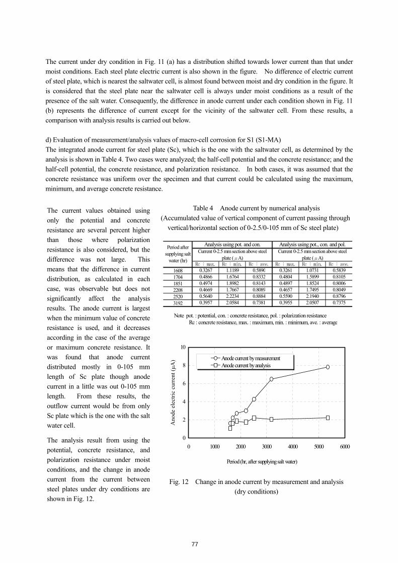
The current under dry condition in Fig. 11 (a) has a distribution shifted towards lower current than that under moist conditions. Each steel plate electric current is also shown in the figure. No difference of electric current of steel plate, which is nearest the saltwater cell, is almost found between moist and dry condition in the figure. It is considered that the steel plate near the saltwater cell is always under moist conditions as a result of the presence of the salt water. Consequently, the difference in anode current under each condition shown in Fig. 11 (b) represents the difference of current except for the vicinity of the saltwater cell. From these results, a comparison with analysis results is carried out below. d) Evaluation of measurement/analysis values of macro-cell corrosion for S1 (S1-MA) The integrated anode current for steel plate (Sc), which is the one with the saltwater cell, as determined by the analysis is shown in Table 4. Two cases were analyzed; the half-cell potential and the concrete resistance; and the half-cell potential, the concrete resistance, and polarization resistance. In both cases, it was assumed that the concrete resistance was uniform over the specimen and that current could be calculated using the maximum, minimum, and average concrete resistance.

Table 4 Anode current by numerical analysis

(Accumulated value of vertical component of current passing through vertical/horizontal section of 0-2.5/0-105 mm of Sc steel plate)

Fig. 12 Change in anode current by measurement and analysis (dry conditions)

Rc : max. Rc : min. Rc : ave. Rc : max. Rc : min. Rc : ave.1608 0.3267 1.1189 0.5890 0.3261 1.0731 0.58391704 0.4866 1.6764 0.8332 0.4804 1.5899 0.81051851 0.4974 1.8982 0.8143 0.4897 1.8524 0.80062208 0.4669 1.7667 0.8089 0.4657 1.7495 0.80492520 0.5640 2.2234 0.8884 0.5590 2.1940 0.87963192 0.3957 2.0584 0.7381 0.3955 2.0507 0.7375

Note pot. : potential, con. : concrete resistance, pol. : polarization resistance Rc : concrete resistance, max. : maximum, min. : minimum, ave. : average

Period aftersupplying salt

water (hr)

Analysis using pot. and con. Analysis using pot., con. and pol.Current 0-2.5 mm section above steel

plate (μA)Current 0-2.5 mm section above steel

plate (μA)

The current values obtained using only the potential and concrete resistance are several percent higher than those where polarization resistance is also considered, but the difference was not large. This means that the difference in current distribution, as calculated in each case, was observable but does not significantly affect the analysis results. The anode current is largest when the minimum value of concrete resistance is used, and it decreases according in the case of the average or maximum concrete resistance. It was found that anode current distributed mostly in 0-105 mm length of Sc plate though anode current in a little was out 0-105 mm length. From these results, the outflow current would be from only Sc plate which is the one with the salt water cell.

The analysis result from using the potential, concrete resistance, and polarization resistance under moist conditions, and the change in anode current from the current between steel plates under dry conditions are shown in Fig. 12.

0

2

4

6

8

10

0 1000 2000 3000 4000 5000 6000

Period (hr, after supplying salt water)

Ano

de e

lect

ric c

urre

nt (µ

A) Anode current by measurement

Anode current by analysis

77

Fig. 13 Relationship between measured and analytical anode current (dry conditions)

The cause of this low analysis value is probably related to concrete resistance. Therefore, it will be necessary in future to carry out a detailed examination of measured concrete resistance and its application in the analysis. If these relations could be sufficiently accurately modeled, the calculated macro-cell corrosion current would be estimated more correctly. e) Evaluation of micro-cell corrosion for S1 As noted already, macro-cell and micro-cell corrosion can be assumed to progress simultaneously. Micro-cell corrosion is examined in this paragraph. In Fig. 14, for specimen S1, the relationship between corrosion current density for each polarization resistance in the connected state (S1-MA-mi) is compared with the disconnected state (S1-mi). Coefficient K in formula (1) is assumed to be 0.026 V on the basis of past reports [10][11][12][13]. In the figure, points surrounded by the ellipse represent the current density for the steel plate with the salt water cell, which is equivalent to the anode, while other points represent the current density of the steel plate equivalent to the cathode. Though the points inside the ellipse are not remarkable as points outside the ellipse, most current densities in the connected are larger than when the steel plates are disconnected. Inside the ellipse, the current obtained from the polarization resistance with connection of lead line, which is considered the anode, represents macro-cell and micro-cell corrosion.

Furthermore, based on the relation in Fig. 12, the relation between anode current by analysis and that measured under dry conditions is shown in Fig. 13. Comparing these results, it is clear that analysis values are lower than the measured ones. The analysis value was about 50-60% of the measured one up to about 2,500 hours, and the difference was about 20-25% after that. It is assumed that the value obtained from the current between steel plates under dry conditions represents the macro-cell corrosion current, and the analysis method applied in this model possibly underestimates the macro-cell current.

y = 2.2589xR2 = 0.5351

0

2

4

6

8

10

0 2 4 6 8 10

Anode current by analysis (µA)

Ano

de c

urre

nt b

y m

easu

rem

ent (

µA)

Fig. 15 Current density from polarization resistance of S1 (steel plate with cell and total of each plate)

Fig. 14 Current density from polarization resistance of S1 (between connected steel plates and dis-connected steel plates)

0.01

0.1

1

10

0.01 0.1 1 10

Current density of dis-connected steel plate (µA/cm2, S1-mi)

Cur

rent

den

sity

of c

onne

cted

stee

l pla

tes (

µA/c

m2,

S1-

MA

-mi)

1608170418512208252031925376

Steel plate with cell

Period (hr)y = 0.2028xR2 = 0.5144

y = 0.9406xR2 = 0.7304

0

2

4

6

8

10

12

14

0 2 4 6 8 10 12 14

Current density of connected steel plates(µA/cm2, S1-MA-mi)

Cur

rent

den

sity

of d

is-c

onne

cted

stee

l pla

te (µ

/cm

2, S

1-m

i) Current density of steel plate with cell

Total current densityof all steel plates

78

The relationship of total current for the connected and disconnected cases is shown in Fig. 15. The total current in the connected case is larger than in the disconnected case by about 5 times. In a continuous steel plate, it is generally difficult to distinguish clearly between the corrosion and non-corrosion part of current density, or between the anode and cathode current, in the case of using potential and polarization resistance measurements. Moreover, there is possibility of mis-assigning the cathode as the anode if using the half-cell potential and the polarization resistance. If the current obtained from the polarization resistance in the cathode part is included, the total corrosion current density should be over estimated because the current density of the anode, which is shown in Figure-14, does not depend on the connection condition. Therefore, in estimating corrosion with mixed macro-cell and micro-cell phenomena, it is easily possible to overestimate the current in the cathode [14]. However, by understanding the relationship shown in Fig. 15, it should be possible to understand micro-cell corrosion under macro-cell conditions. f) Estimation of corrosion quantity and mass loss by corrosion The final process is to calculate the total amount of corrosion from the accumulated corrosion amount analyzed under each condition for S1 and L1. The result is shown in Table 5. The results presented in Table 5, and the relationship between the change in corrosion quantity and mass loss are shown in Fig. 16 (a) and (b). The analysis result and the measurement of corrosion mass loss was limited to the region of the plate with a salt water cell on both S1 and L1 (the length of L1 is equal to the length of Sc part of S1). As described in the section 2.(4)(a), it was expected that the corrosion mass loss would be affected by loss of resin coating and the influence of mortar adhesion, but no influences were seen. When the plates in S1 were connected in this model test, the corrosion quantity determined from the reciprocal of polarization resistance was a little larger than during temporary disconnection of the plates, but the difference was not very great. In fact, the corrosion loss obtained with disconnection is equal to or more than 90 % of that obtained from polarization resistance in the connection state, so the difference in corrosion quantity is several percent at most.

Table 5 Relation between estimated corrosion loss by analysis and measured mass loss due to corrosion (unit: mg)

Ana-MA Mea-dry-MA *-mi *-MA-mi Est.-tot-cor. MLSC

S1

8.424 : A 23.750 : B

From A and B,

Mea-dry-MA/Ana-MA=2.82 : F

96.453 : C 97.522 : D

From C and D, S1-mi/S1-MA-mi=0.989 : G

From B + C 120.204 : E

123.300

L1

4.574 : H From F and H

12.899 : J From G and I

50.158 : K 50.714 : I From J + K 63.057 71.400

Note) Ana.-MA: Macro-cell corrosion loss by analysis, Mea.-dry-MA: Macro-cell corrosion loss by measurement under

dry conditions, S1-mi, S1-MA･mi: Corrosion loss from polarization resistance with connected/disconnected S1, Est.-tot.-cor.: Total corrosion loss by estimation , MLSC: Mass loss of steel through corrosion by measurement

*: Both of S1 and L1，and L1-mi was obtained from estimated L1-MA-mi by relationship S1-MA-mi and S1-mi In Fig.16 (a) and Table 5, it is supposed that the corrosion loss of S1 with disconnection is the micro-cell corrosion, whereas the corrosion loss obtained from the current between the steel plates under dry conditions is the macro-cell corrosion quantity. The total amount of corrosion was calculated to be 120.2 mg, a value near the

79

actual corrosion loss of 123.3 mg. On the other hand, in Fig. 16 (b) and Table-5, the accumulation corrosion loss obtained from the reciprocal of the polarization resistance on the steel plate near the salt water cell of L1 was 50.7 mg. From the relation between connected and disconnected time for S1, this 50.2 mg is converted into the micro-cell corrosion. The macro-cell corrosion loss obtained by analysis of L1 was calculated from the ratio explained below. The analysis macro-cell corrosion of L1 was multiplied by the ratio of macro-cell corrosion quantity of S1 between measurement under dry condition and analysis. Based on this result, the total corrosion loss by calculation is 63.1 mg, and this is about 88% of the actual corrosion loss of 72.1 mg. Though the estimate value is lower than the actual value, the calculation can be considered suitable for evaluating the corrosion of continuous steel material using something like the S1 model (with connected and temporary disconnected short steel plates). In particular, to specify the corrosion accurately, it is possible to estimate the total corrosion loss by taking the macro-cell corrosion from analysis and the micro-cell corrosion obtained from the polarization resistance near the corroded area. This means that, in order to examine steel corrosion in concrete structures, it will be necessary to go through the following steps: (1) obtain the current distribution due to macro-cell corrosion from measurements such as the half-cell potential, the polarization resistance, and the concrete resistance, the definite boundaries of the anode and cathode regions, and an estimate of macro-cell corrosion loss (2) obtain an estimate of micro-cell corrosion loss from the reciprocal of the polarization resistance in the anode area, which is obtained from (1) (3) estimate the total corrosion loss from the relation between (1) and (2) On the other hand, though the rate of micro-cell corrosion is large in the model test, this may result from the indoor dry environment to which the specimen was exposed. Thus, it can be assumed that there was little development of macro-cell corrosion. In work to follow, it will be necessary to examine the repeatability of these macro-cell corrosion analysis results and the choice of coefficient K for determining corrosion from the reciprocal of polarization resistance. Further, it will be necessary to carry out more detailed examinations, such as experiments under various levels of salinity including a case where the main loss is macro-cell corrosion. (a) Corrosion loss by estimation and steel mass loss (b) Corrosion loss by estimation and steel mass loss

by corrosion (S1) by corrosion (L1)

Fig. 16 Corrosion loss by estimation and steel mass loss by corrosion (S1 and L1)

0

10

20

30

40

50

60

70

80

0 1000 2000 3000 4000 5000 6000

Period (hr)

Cor

rosi

on lo

ss (m

g)

Macro-cell corrosion by estimation

Micro-cell corrosion by estimation

Corrosion loss by estimation

Steel mass loss through corrosion by measurement

Accumulated macro-cellcorrosion by numericalanalysis

Accumulated corrosion lossfrom reciprocal ofpolarization resistance

0

20

40

60

80

100

120

140

0 1000 2000 3000 4000 5000 6000

Period (hr)

Cor

rosi

on lo

ss (m

g)

From current under dry conditionsFrom current by numerical analysisFrom current by polarization resistance with connected lineFrom current by polarization resistance with disconnected line

Corrosion loss by estimation

Steel mass loss by corrosion

Estimation cases

80

4. CONCLUSIONS A model test in which the corroded area was made small was carried out, and steel corrosion in the concrete was evaluated using non-destructive methods and a numerical analysis. The following conclusions were reached through this study: (1) Specimens were exposed under water and dry environments for a constant period, and continuous supply of salt water was provided to a salt water cell. During this period, the rate of corrosion of steel plates could be specified by non-destructive methods such as the half-cell potential, polarization resistance, and concrete resistance. (2) In the case of macro-cell corrosion analysis of two types of specimen, L1 and S1, a difference in current distribution arose between the case where only half-cell potential and the concrete resistance were considered and the case where polarization resistance was also added as an analytical factor. However, there was no significant difference in the total anode current. (3) In connecting the leads in specimen S1, the difference between anode current from the analysis and the measured value of current between the steel plates was large in some cases, but the relationship can be understood. (4) In connecting the leads in specimen S1 and then disconnecting them temporarily, the current density from the polarization resistance is large when the connection is near the cell where corrosion takes place. However, this difference of current density was small, and, in another place except the place near the cell, the value in the connected case is larger than when disconnected. (5) In case of the model tests in this study, the micro-cell corrosion accounted for large proportion of all corrosion loss. This is considered a result of the specimen being indoors in dry condition; this environmental affected the result. (6) The corrosion quantity determined from polarization resistance when the leads in specimen S1 were temporarily disconnected is micro-cell corrosion. On the other hand, the corrosion loss obtained by examining the relation between analysis value and measured value of macro-cell current when the S1 leads were connected is macro-cell corrosion. It is possible to estimate the total corrosion loss, and to estimate the macro/micro-cell corrosion loss of L1, using the same general method. From results of this study, it seems difficult to understand steel corrosion only in terms of polarization resistance measured in various locations. Rather, it is necessary to estimate the macro-cell and micro-cell corrosion after distinguishing the anode and cathode accurately through measurements such as half-cell potential, polarization resistance and concrete resistance, and through analysis of macro-cell corrosion. On the other hand, the repeatability of macro-cell analysis and the application of K to micro-cell analysis affect the estimation of corrosion. Thus, a detailed examination of behavior under various salinity levels will be necessary in the future.

81

Acknowledgement We appreciate the many valuable suggestions made by Dr. Masaru Yokota, chief researcher at Shikoku Research Institute, Inc. References [1] 305 Committee: Present status and trend in the study of corrosion/anti-corrosion of reinforcing steel and its repair, The corrosion/anti-corrosion subcommittee report of the concrete committee, Concrete engineering series 26, JSCE, 1997 (in Japanese) [2] Miyagawa, T.: Early chloride corrosion of reinforcing steel in concrete, Kyoto University Doctoral Thesis, 1985 [3] Koyama, R., Yajima, T., Uomoto, T., and Hoshino, T.: Prediction of steel corrosion portion and area by natural potential measurement, Journal of Materials, Concrete Structures and Pavements, JSCE, No.550/V-33, pp.13-21, 1996 (in Japanese) [4] Nagataki, S., Otsuki, N., Moriwake, A., and Miyazato S.: The experimental study on corrosion mechanism of reinforced concrete at local repair part, Journal of Materials, Concrete Structures and Pavements, JSCE, No.544/V-32, pp.109-119, 1996 (in Japanese) [5]Yokota, M., and Tamura, H.: Electrochemical nondestructive inspection for corrosion diagnosis of reinforcement in concrete structures, Journal of Nondestructive Inspection, Vol. 47, No.9, pp.649-654, 1998 (in Japanese) [6] Elsener, B.: Corrosion rate of steel in concrete from laboratory to reinforced structures，Materials Science Forum, Vol.247, pp.127-138, 1997 [7] Kobayashi, K., and Miyagawa, T.: Study on estimation of corrosion rate of reinforcing steel in concrete by measuring polarization resistance, Journal of Materials, Concrete Structures and Pavements, JSCE, No.669/V-50, pp.173-186, 2001 (in Japanese) [8] Translated by Honma, T., and Tanaka, Y.: Written by Silvester, P. P., and Ferrari, R. L. “Finite Elements for Electrical Engineers”, Science, 1988 (in Japanese) [9] Seki, H., Miyata, K., Kitamine, H., and Kaneko, Y.: Experimental study on permeability of concrete based on electrical resistivity, Concrete Engineering and Pavements, JSCE, No.451/V-17, pp.49-57, 1992 (in Japanese) [10] Okada, K., Kobayashi, K., Miyagawa, T., and Honda, T.: Repair standards by reinforcing steel corrosion monitoring using a polarization resistance method, Proceedings of JCI 5th Conference, pp.249-252, 1983 (in Japanese) [11] Yokota, M.: Estimation of corrosion behavior for steel rebar in concrete by electrochemical methods, Proceedings of JCI, Vol.12, No.1, pp.545-550, 1990 (in Japanese) [12] Flis, J., Sabol, S., Pickering, H. W., Sehgal, A., Osseo-Asare, K., and Cady, P. D.: Electro-chemical Measurements on Concrete Bridges for Evaluation of Reinforcement Corrosion Rates, Corrosion, Vol.49, No.7, pp.601-613, 1993 [13] Andrade, C., Castelo, V., Alonso, C., and Gonzalez, J. A.: The determination of the corrosion rate of steel embedded in concrete by the polarization resistance and AC impedance methods, Proc. Int. Symp., Williamsburg, USA, ASTM STP 906, pp.43-63, 1986 [14] Gulikers, J.: Numerical simulation of corrosion rate determination by linear polarization, measurement and interpretation of the on-site corrosion rate, Proc. of Int. Workshop MESINA, Madrid, Spain, RILEM Publications, pp.145-156, 1999

82