A Study of Convective Velocity in Supersonic Jets Using ... · American Institute of Aeronautics and Astronautics 2 The last couple of decades have produced many empirical studies

American Institute of Aeronautics and Astronautics

1

A Study of Convective Velocity in Supersonic Jets Using

MHz Rate Imaging

M. Blohm*, W. Lempert

†, and M. Samimy

‡

Gas Dynamics and Turbulence Laboratory

The Ohio State University, Columbus, OH, 43235, USA

and

B. Thurow§

Auburn University, Auburn, Alabama, 36849

MHz-rate flow visualization and Planar Doppler Velocimetry (PDV) measurements were

carried out in Mach 1.3 and 2.0 axisymmetric jets with Reynolds number based on the nozzle exit

diameter of over 106 using a burst mode laser and a pair of high-speed CCD framing cameras.

Determination of convective velocity from flow visualization using planar space-time correlation

reveals strong evidence of bias due to distinct artificial seeding gradients resulting from partial

seeding of the flow (i.e. seeding of the mixing region, but not the jet core and the ambient). This

bias can be somewhat rectified if the measurements are restricted to the early part of the shear

layer growth, where the structures are relatively coherent and the correlation level is high and

contains a distinct peak. The bias can be nearly eliminated if the entire flow field is seeded and

PDV, rather than flow visualization, is used to determine the convective velocity. Under these

circumstances, the measured convective velocity agrees very well with theoretical predictions.

I. Introduction

he study of compressible shear layers has been motivated by their importance to many practical engineering

applications such as noise production and high speed fuel/air mixing. Although it was not initially intended, the

incompressible free shear layer work of Brown and Roshko [1974] was the first to display the presence of large-

scale vortical structures in such flows of high Reynolds numbers. The theoretical work of Bogdanoff [1983] and

experimental work of Papamoschou and Roshko [1988] extended the work in incompressible free shear layers to

compressible cases and defined a convective Mach number, Mc, and corresponding convective velocity as:

2

2

1

1

21

21

a

UU

a

UU

aa

UUM cc

c

−=

−=

+

−=

(1)

21

2211

aa

UaUaU c

+

+=

(2)

where U is the free stream velocity, a is the speed of sound, and the subscripts 1 and 2 indicate the high and low

speed streams, respectively.

It was shown both in the theoretical study of Bogandoff [1983] and the experimental study of Papamoschou and

Roshko [1988] that this convective Mach number correlated the shear layer growth rate and thus has been used

extensively as an important compressibility parameter.

* Graduate Student, AIAA member; Currently with GE Energy – Gas Turbine Compressor Aerodynamics † Professor, Dept. of Mechanical Eng. and Chemistry, AIAA Associate Fellow ‡ Professor, Dept. of Mechanical Eng., Director, Gas Dynamics and Turbulence Laboratory, AIAA Associate

Fellow, corresponding author: [email protected] § Assistant Professor, Dept. of Aerospace Eng., AIAA member

T

44th AIAA Aerospace Sciences Meeting and Exhibit9 - 12 January 2006, Reno, Nevada

AIAA 2006-45

Copyright © 2006 by the American Institute of Aeronautics and Astronautics, Inc. All rights reserved.


2

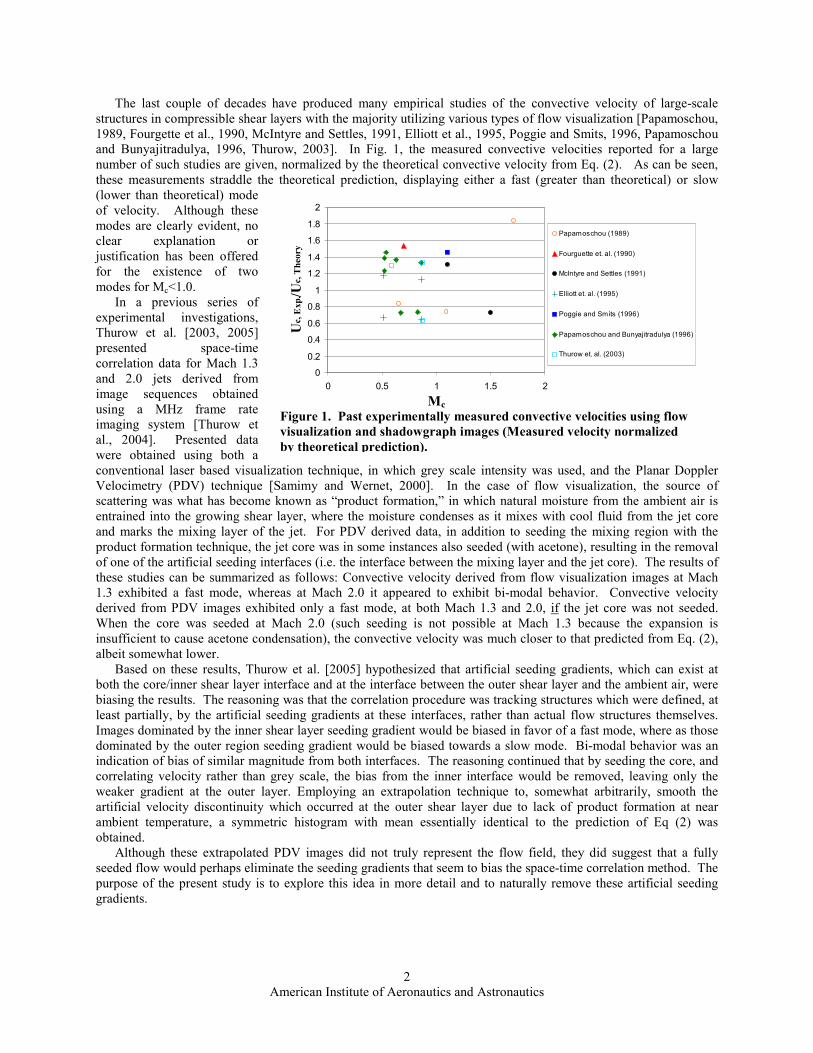
The last couple of decades have produced many empirical studies of the convective velocity of large-scale

structures in compressible shear layers with the majority utilizing various types of flow visualization [Papamoschou,

1989, Fourgette et al., 1990, McIntyre and Settles, 1991, Elliott et al., 1995, Poggie and Smits, 1996, Papamoschou

and Bunyajitradulya, 1996, Thurow, 2003]. In Fig. 1, the measured convective velocities reported for a large

number of such studies are given, normalized by the theoretical convective velocity from Eq. (2). As can be seen,

these measurements straddle the theoretical prediction, displaying either a fast (greater than theoretical) or slow

(lower than theoretical) mode

of velocity. Although these

modes are clearly evident, no

clear explanation or

justification has been offered

for the existence of two

modes for Mc<1.0.

In a previous series of

experimental investigations,

Thurow et al. [2003, 2005]

presented space-time

correlation data for Mach 1.3

and 2.0 jets derived from

image sequences obtained

using a MHz frame rate

imaging system [Thurow et

al., 2004]. Presented data

were obtained using both a

conventional laser based visualization technique, in which grey scale intensity was used, and the Planar Doppler

Velocimetry (PDV) technique [Samimy and Wernet, 2000]. In the case of flow visualization, the source of

scattering was what has become known as “product formation,” in which natural moisture from the ambient air is

entrained into the growing shear layer, where the moisture condenses as it mixes with cool fluid from the jet core

and marks the mixing layer of the jet. For PDV derived data, in addition to seeding the mixing region with the

product formation technique, the jet core was in some instances also seeded (with acetone), resulting in the removal

of one of the artificial seeding interfaces (i.e. the interface between the mixing layer and the jet core). The results of

these studies can be summarized as follows: Convective velocity derived from flow visualization images at Mach

1.3 exhibited a fast mode, whereas at Mach 2.0 it appeared to exhibit bi-modal behavior. Convective velocity

derived from PDV images exhibited only a fast mode, at both Mach 1.3 and 2.0, if the jet core was not seeded.

When the core was seeded at Mach 2.0 (such seeding is not possible at Mach 1.3 because the expansion is

insufficient to cause acetone condensation), the convective velocity was much closer to that predicted from Eq. (2),

albeit somewhat lower.

Based on these results, Thurow et al. [2005] hypothesized that artificial seeding gradients, which can exist at

both the core/inner shear layer interface and at the interface between the outer shear layer and the ambient air, were

biasing the results. The reasoning was that the correlation procedure was tracking structures which were defined, at

least partially, by the artificial seeding gradients at these interfaces, rather than actual flow structures themselves.

Images dominated by the inner shear layer seeding gradient would be biased in favor of a fast mode, where as those

dominated by the outer region seeding gradient would be biased towards a slow mode. Bi-modal behavior was an

indication of bias of similar magnitude from both interfaces. The reasoning continued that by seeding the core, and

correlating velocity rather than grey scale, the bias from the inner interface would be removed, leaving only the

weaker gradient at the outer layer. Employing an extrapolation technique to, somewhat arbitrarily, smooth the

artificial velocity discontinuity which occurred at the outer shear layer due to lack of product formation at near

ambient temperature, a symmetric histogram with mean essentially identical to the prediction of Eq (2) was

obtained.

Although these extrapolated PDV images did not truly represent the flow field, they did suggest that a fully

seeded flow would perhaps eliminate the seeding gradients that seem to bias the space-time correlation method. The

purpose of the present study is to explore this idea in more detail and to naturally remove these artificial seeding

gradients.

0

0.2

0.4

0.6

0.8

1

1.2

1.4

1.6

1.8

2

0 0.5 1 1.5 2

Mc

Uc,

Exp

. /Uc,

Th

eory

Papamoschou (1989)

Fourguette et. al. (1990)

McIntyre and Settles (1991)

Elliott et. al. (1995)

Poggie and Smits (1996)

Papamoschou and Bunyajitradulya (1996)

Thurow et. al. (2003)

Figure 1. Past experimentally measured convective velocities using flow

visualization and shadowgraph images (Measured velocity normalized

by theoretical prediction).


3

II. Experimental Facilities and Methods

All PDV and flow visualization images were recorded in the Ohio State University’s Gas Dynamics and

Turbulence Laboratory (GDTL). The facility contains a stagnation plenum and jet stand equipped with a variety of

nozzles, designed via the method of characteristics. The free jet exits from the test nozzle and is exhausted through

a large bell mouth, located approximately 8 ft. from the nozzle exit. The two jets investigated in this experiment are

Mach 1.3 and 2.0, identical to those studied by Thurow et al. [2003, 2005], with Reynolds numbers based on nozzle

exit diameter of 1.0 × 106 and 2.4 × 10

6, respectively.

The MHz frame rate flow visualization and PDV instrumentation employed in this work have been described in

detail previously and will therefore be only summarized here. The illumination source is a second-generation “pulse

burst” laser system [Thurow, et al., 2004], which has been shown to produce burst trains of 10-30 pulses with

spacing as low as 1 microsecond and individual pulse energies as high as 100 mJ. For the measurements to be

presented here, the burst train was composed of 28 pulses (~10ns FWHM) with 4 µs inter-pulse spacing. The

average individual pulse energy at the second harmonic wavelength of 0.532µm was ~ 10 mJ, which was more than sufficient. Images were acquired using two ultra high frame rate CCD cameras (Model PSI-IV) manufactured by

Princeton Scientific Instruments. The cameras have a pixel format of 81 × 161, and can capture up to 28 frames

with framing rate as high as 1 ΜΗz. The high frame rate is achieved by continuous shifting of charge from each individual pixel into its own on-chip 28 frame memory storage area. Upon receipt of a stop trigger, the last 28

frames obtained are transferred to a PC for subsequent post processing.

The PDV technique has also been described in detail elsewhere [Samimy and Wernet, 2000]. The basic concept

utilizes the Doppler shift of scattered light, which is a function of scattering particle velocity and optical geometry

according to

Vos

fDv

rr

⋅−

=∆λ

)( (3)

where sr and o

r are the unit vectors in the scattered and incident laser propagation directions, respectively, λ is the

wavelength of light, and Vris the flow velocity vector. For all the experimental results to be presented here, a 1–

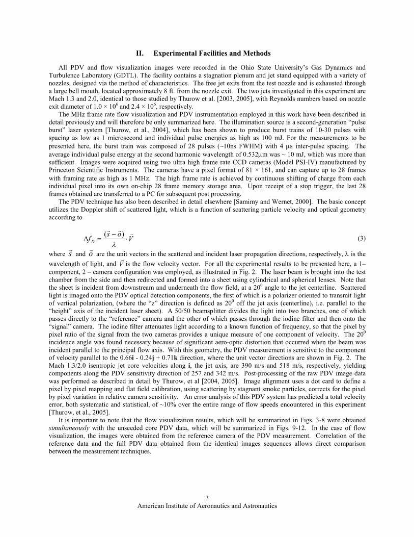
component, 2 – camera configuration was employed, as illustrated in Fig. 2. The laser beam is brought into the test

chamber from the side and then redirected and formed into a sheet using cylindrical and spherical lenses. Note that

the sheet is incident from downstream and underneath the flow field, at a 200 angle to the jet centerline. Scattered

light is imaged onto the PDV optical detection components, the first of which is a polarizer oriented to transmit light

of vertical polarization, (where the “z” direction is defined as 200 off the jet axis (centerline), i.e. parallel to the

“height” axis of the incident laser sheet). A 50/50 beamsplitter divides the light into two branches, one of which

passes directly to the “reference” camera and the other of which passes through the iodine filter and then onto the

“signal” camera. The iodine filter attenuates light according to a known function of frequency, so that the pixel by

pixel ratio of the signal from the two cameras provides a unique measure of one component of velocity. The 200

incidence angle was found necessary because of significant aero-optic distortion that occurred when the beam was

incident parallel to the principal flow axis. With this geometry, the PDV measurement is sensitive to the component

of velocity parallel to the 0.66i - 0.24j + 0.71k direction, where the unit vector directions are shown in Fig. 2. The

Mach 1.3/2.0 isentropic jet core velocities along i, the jet axis, are 390 m/s and 518 m/s, respectively, yielding

components along the PDV sensitivity direction of 257 and 342 m/s. Post-processing of the raw PDV image data

was performed as described in detail by Thurow, et al [2004, 2005]. Image alignment uses a dot card to define a

pixel by pixel mapping and flat field calibration, using scattering by stagnant smoke particles, corrects for the pixel

by pixel variation in relative camera sensitivity. An error analysis of this PDV system has predicted a total velocity

error, both systematic and statistical, of ~10% over the entire range of flow speeds encountered in this experiment

[Thurow, et al., 2005].

It is important to note that the flow visualization results, which will be summarized in Figs. 3-8 were obtained

simultaneously with the unseeded core PDV data, which will be summarized in Figs. 9-12. In the case of flow

visualization, the images were obtained from the reference camera of the PDV measurement. Correlation of the

reference data and the full PDV data obtained from the identical images sequences allows direct comparison

between the measurement techniques.


4

Figure 2. Schematic diagram illustrating laser sheet, jet, and PDV optical components.

The correlation technique utilizes the fluctuating signal defined by:

),(),,(),,(' yxFtyxFtyxF kkkk −= (4)

where ),,( kk tyxF is the time varying signal and ),( yxF is the ensemble average. For an x, y array of

fluctuating signals in time (i.e. an image), the average correlation, C, between two of these instances (i,j) is given as:

),,('),,('1

1 1

, jj

m

x

n

y

iiji tyxFtyxFmn

C ∑∑= =

= (5)

where m and n are the pixel index in the x and y directions, respectively. In practice Eq. (5) needs to reflect the

displacement of structures being tracked, resulting in,

),,('),,('1

),(1 1

, jj

m

x

n

y

iiji tyyxxFtyxFmn

yxC ∆+∆+=∆∆ ∑∑= =

(6)

Sig. Cam.

Jet Nozzle

Laser Sheet

Beam from

PBL

Ref. Cam.

Polarizer

50/50 Beamsplitter Mirror

Iodine Filter

Scattered Light

(Frequency Shifted)

Illuminated

Flow Field

k is out of plane i

j

20°

Incident laser sheet direction

sv


5

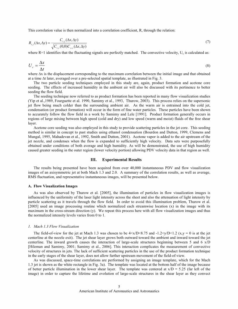
This correlation value is then normalized into a correlation coefficient, R, through the relation:

),()0,0(

),(),(

,,

,

,yxCC

yxCyxR

jjji

ji

ji∆∆

∆∆=∆∆ (7)

where R=1 identifies that the fluctuating signals are perfectly matched. The convective velocity, Uc is calculated as:

t

xU c

∆

∆= (8)

where ∆x is the displacement corresponding to the maximum correlation between the initial image and that obtained

at a time ∆t later, averaged over a pre-selected spatial template, as illustrated in Fig. 3.

The two particle seeding techniques employed in this study are, again, product formation and acetone core

seeding. The effects of increased humidity in the ambient air will also be discussed with its pertinence to better

seeding the flow field.

The seeding technique now referred to as product formation has been reported in many flow visualization studies

(Yip et al.,1989, Fourguette et al. 1990, Samimy et al., 1993, Thurow, 2003). This process relies on the supersonic

jet flow being much colder than the surrounding ambient air. As the warm air is entrained into the cold jet,

condensation (or product formation) will occur in the form of fine water particles. These particles have been shown

to accurately follow the flow field in a work by Samimy and Lele [1991]. Product formation generally occurs in

regions of large mixing between high speed (cold and dry) and low speed (warm and moist) fluids of the free shear

layer.

Acetone core seeding was also employed in this study to provide scattering particles in the jet core. This seeding

method is similar in concept to past studies using ethanol condensation (Bourdon and Dutton, 1999, Clemens and

Mungal, 1995, Mahadevan et al., 1992, Smith and Dutton, 2001). Acetone vapor is added to the air upstream of the

jet nozzle, and condenses when the flow is expanded to sufficiently high velocity. Data sets were purposefully

obtained under conditions of both average and high humidity. As will be demonstrated, the use of high humidity

caused greater seeding in the outer region (lower velocity portion) allowing PDV velocity data in that region as well.

III. Experimental Results

The results being presented have been acquired from over 40,000 instantaneous PDV and flow visualization

images of an axisymmetric jet at both Mach 1.3 and 2.0. A summary of the correlation results, as well as average,

RMS fluctuation, and representative instantaneous images, will be presented below.

A. Flow Visualization Images

As was also observed by Thurow et al. [2005], the illumination of particles in flow visualization images is

influenced by the uniformity of the laser light intensity across the sheet and also the attenuation of light intensity by

particle scattering as it travels through the flow field. In order to avoid this illumination problem, Thurow et al.

[2005] used an image processing routine which normalized each streamwise location (x) in the image with its

maximum in the cross-stream direction (y). We repeat this process here with all flow visualization images and thus

the normalized intensity levels varies from 0 to 1.

1. Mach 1.3 Flow Visualization

The field-of-view for the jet at Mach 1.3 was chosen to be 4<x/D<8.75 and -1.2<y/D<1.2 (x,y = 0 is at the jet

centerline at the nozzle exit). The jet shear layer grows both outward toward the ambient and inward toward the jet

centerline. The inward growth causes the interaction of large-scale structures beginning between 5 and 6 x/D

[Hileman and Samimy, 2001; Samimy et al., 2006]. This interaction complicates the measurement of convective

velocity of structures in jets. The lack of sufficient scattering particles in the use of the product formation technique

in the early stages of the shear layer, does not allow further upstream movement of the field-of-view.

As was discussed, space-time correlations are performed by assigning an image template, which for the Mach

1.3 jet is shown as the white rectangle in Fig. 3a). The template was located at the bottom half of the image because

of better particle illumination in the lower shear layer. The template was centered at x/D = 5.25 (far left of the

image) in order to capture the lifetime and evolution of large-scale structures in the shear layer as they convect


6

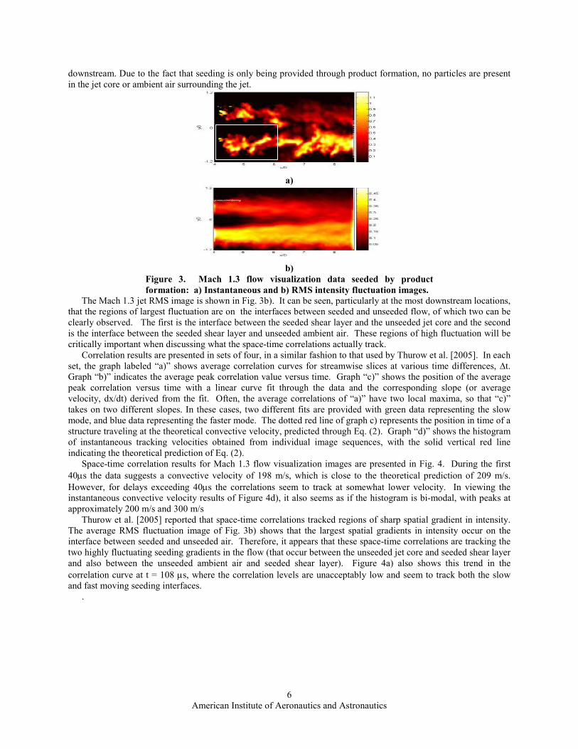
downstream. Due to the fact that seeding is only being provided through product formation, no particles are present

in the jet core or ambient air surrounding the jet.

a)

b)

Figure 3. Mach 1.3 flow visualization data seeded by product

formation: a) Instantaneous and b) RMS intensity fluctuation images.

The Mach 1.3 jet RMS image is shown in Fig. 3b). It can be seen, particularly at the most downstream locations,

that the regions of largest fluctuation are on the interfaces between seeded and unseeded flow, of which two can be

clearly observed. The first is the interface between the seeded shear layer and the unseeded jet core and the second

is the interface between the seeded shear layer and unseeded ambient air. These regions of high fluctuation will be

critically important when discussing what the space-time correlations actually track.

Correlation results are presented in sets of four, in a similar fashion to that used by Thurow et al. [2005]. In each

set, the graph labeled “a)” shows average correlation curves for streamwise slices at various time differences, ∆t.

Graph “b)” indicates the average peak correlation value versus time. Graph “c)” shows the position of the average

peak correlation versus time with a linear curve fit through the data and the corresponding slope (or average

velocity, dx/dt) derived from the fit. Often, the average correlations of “a)” have two local maxima, so that “c)”

takes on two different slopes. In these cases, two different fits are provided with green data representing the slow

mode, and blue data representing the faster mode. The dotted red line of graph c) represents the position in time of a

structure traveling at the theoretical convective velocity, predicted through Eq. (2). Graph “d)” shows the histogram

of instantaneous tracking velocities obtained from individual image sequences, with the solid vertical red line

indicating the theoretical prediction of Eq. (2).

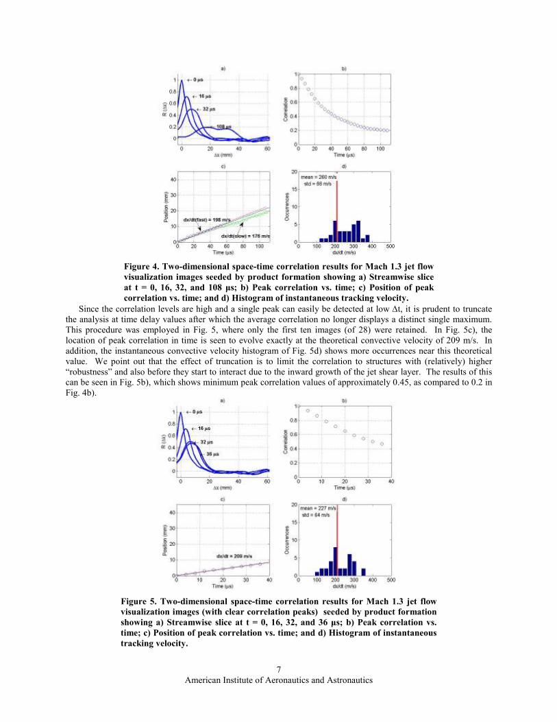
Space-time correlation results for Mach 1.3 flow visualization images are presented in Fig. 4. During the first

40µs the data suggests a convective velocity of 198 m/s, which is close to the theoretical prediction of 209 m/s.

However, for delays exceeding 40µs the correlations seem to track at somewhat lower velocity. In viewing the instantaneous convective velocity results of Figure 4d), it also seems as if the histogram is bi-modal, with peaks at

approximately 200 m/s and 300 m/s

Thurow et al. [2005] reported that space-time correlations tracked regions of sharp spatial gradient in intensity.

The average RMS fluctuation image of Fig. 3b) shows that the largest spatial gradients in intensity occur on the

interface between seeded and unseeded air. Therefore, it appears that these space-time correlations are tracking the

two highly fluctuating seeding gradients in the flow (that occur between the unseeded jet core and seeded shear layer

and also between the unseeded ambient air and seeded shear layer). Figure 4a) also shows this trend in the

correlation curve at t = 108 µs, where the correlation levels are unacceptably low and seem to track both the slow and fast moving seeding interfaces.

.


7

Figure 4. Two-dimensional space-time correlation results for Mach 1.3 jet flow

visualization images seeded by product formation showing a) Streamwise slice

at t = 0, 16, 32, and 108 µs; b) Peak correlation vs. time; c) Position of peak

correlation vs. time; and d) Histogram of instantaneous tracking velocity.

Since the correlation levels are high and a single peak can easily be detected at low ∆t, it is prudent to truncate the analysis at time delay values after which the average correlation no longer displays a distinct single maximum.

This procedure was employed in Fig. 5, where only the first ten images (of 28) were retained. In Fig. 5c), the

location of peak correlation in time is seen to evolve exactly at the theoretical convective velocity of 209 m/s. In

addition, the instantaneous convective velocity histogram of Fig. 5d) shows more occurrences near this theoretical

value. We point out that the effect of truncation is to limit the correlation to structures with (relatively) higher

“robustness” and also before they start to interact due to the inward growth of the jet shear layer. The results of this

can be seen in Fig. 5b), which shows minimum peak correlation values of approximately 0.45, as compared to 0.2 in

Fig. 4b).


visualization images (with clear correlation peaks) seeded by product formation

showing a) Streamwise slice at t = 0, 16, 32, and 36 µs; b) Peak correlation vs.

time; c) Position of peak correlation vs. time; and d) Histogram of instantaneous

tracking velocity.


8

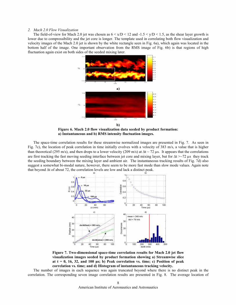
2. Mach 2.0 Flow Visualization

The field-of-view for Mach 2.0 jet was chosen as 6 < x/D < 12 and -1.5 < y/D < 1.5, as the shear layer growth is

lower due to compressibility and the jet core is longer. The template used in correlating both flow visualization and

velocity images of the Mach 2.0 jet is shown by the white rectangle seen in Fig. 6a), which again was located in the

bottom half of the image. One important observation from the RMS image of Fig. 6b) is that regions of high

fluctuation again exist on both sides of the seeded mixing later.

a)

b)

Figure 6. Mach 2.0 flow visualization data seeded by product formation:

a) Instantaneous and b) RMS intensity fluctuation images.

The space-time correlation results for these streamwise normalized images are presented in Fig. 7. As seen in

Fig. 7c), the location of peak correlation in time initially evolves with a velocity of 383 m/s, a value that is higher

than theoretical (295 m/s), and then drops to a lower velocity (209 m/s) at ∆t ~ 72 µs. It appears that the correlations

are first tracking the fast moving seeding interface between jet core and mixing layer, but for ∆t >~72 µs they track the seeding boundary between the mixing layer and ambient air. The instantaneous tracking results of Fig. 7d) also

suggest a somewhat bi-modal nature, however, there seem to be more fast mode than slow mode values. Again note

that beyond ∆t of about 72, the correlation levels are low and lack a distinct peak.


visualization images seeded by product formation showing a) Streamwise slice

at t = 0, 16, 32, and 100 µs; b) Peak correlation vs. time; c) Position of peak


The number of images in each sequence was again truncated beyond where there is no distinct peak in the

correlation. The corresponding seven image correlation results are presented in Fig. 8. The average location of


9

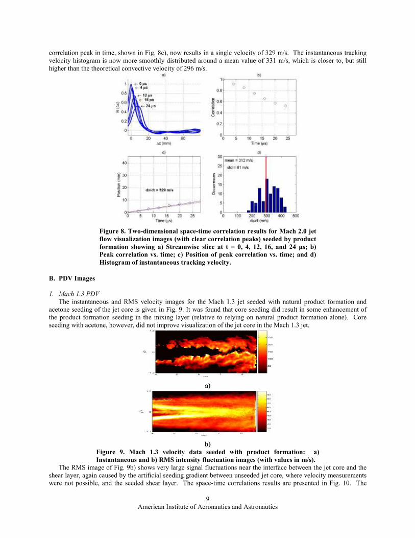
correlation peak in time, shown in Fig. 8c), now results in a single velocity of 329 m/s. The instantaneous tracking

velocity histogram is now more smoothly distributed around a mean value of 331 m/s, which is closer to, but still

higher than the theoretical convective velocity of 296 m/s.

Figure 8. Two-dimensional space-time correlation results for Mach 2.0 jet

flow visualization images (with clear correlation peaks) seeded by product

formation showing a) Streamwise slice at t = 0, 4, 12, 16, and 24 µs; b)

Peak correlation vs. time; c) Position of peak correlation vs. time; and d)

Histogram of instantaneous tracking velocity.

B. PDV Images

1. Mach 1.3 PDV

The instantaneous and RMS velocity images for the Mach 1.3 jet seeded with natural product formation and

acetone seeding of the jet core is given in Fig. 9. It was found that core seeding did result in some enhancement of

the product formation seeding in the mixing layer (relative to relying on natural product formation alone). Core

seeding with acetone, however, did not improve visualization of the jet core in the Mach 1.3 jet.

a)

b)

Figure 9. Mach 1.3 velocity data seeded with product formation: a)

Instantaneous and b) RMS intensity fluctuation images (with values in m/s).

The RMS image of Fig. 9b) shows very large signal fluctuations near the interface between the jet core and the

shear layer, again caused by the artificial seeding gradient between unseeded jet core, where velocity measurements

were not possible, and the seeded shear layer. The space-time correlations results are presented in Fig. 10. The


10

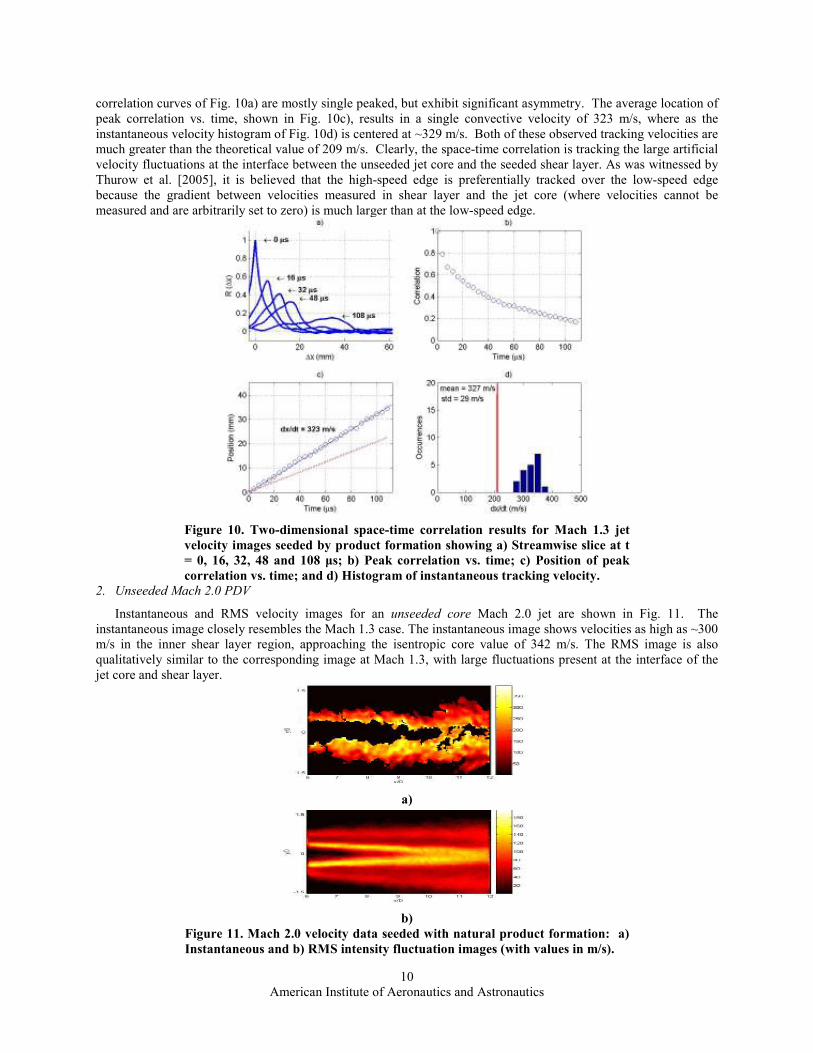
correlation curves of Fig. 10a) are mostly single peaked, but exhibit significant asymmetry. The average location of

peak correlation vs. time, shown in Fig. 10c), results in a single convective velocity of 323 m/s, where as the

instantaneous velocity histogram of Fig. 10d) is centered at ~329 m/s. Both of these observed tracking velocities are

much greater than the theoretical value of 209 m/s. Clearly, the space-time correlation is tracking the large artificial

velocity fluctuations at the interface between the unseeded jet core and the seeded shear layer. As was witnessed by

Thurow et al. [2005], it is believed that the high-speed edge is preferentially tracked over the low-speed edge

because the gradient between velocities measured in shear layer and the jet core (where velocities cannot be

measured and are arbitrarily set to zero) is much larger than at the low-speed edge.


velocity images seeded by product formation showing a) Streamwise slice at t

= 0, 16, 32, 48 and 108 µs; b) Peak correlation vs. time; c) Position of peak


2. Unseeded Mach 2.0 PDV

Instantaneous and RMS velocity images for an unseeded core Mach 2.0 jet are shown in Fig. 11. The

instantaneous image closely resembles the Mach 1.3 case. The instantaneous image shows velocities as high as ~300

m/s in the inner shear layer region, approaching the isentropic core value of 342 m/s. The RMS image is also

qualitatively similar to the corresponding image at Mach 1.3, with large fluctuations present at the interface of the

jet core and shear layer.

a)

b)

Figure 11. Mach 2.0 velocity data seeded with natural product formation: a)

Instantaneous and b) RMS intensity fluctuation images (with values in m/s).


11

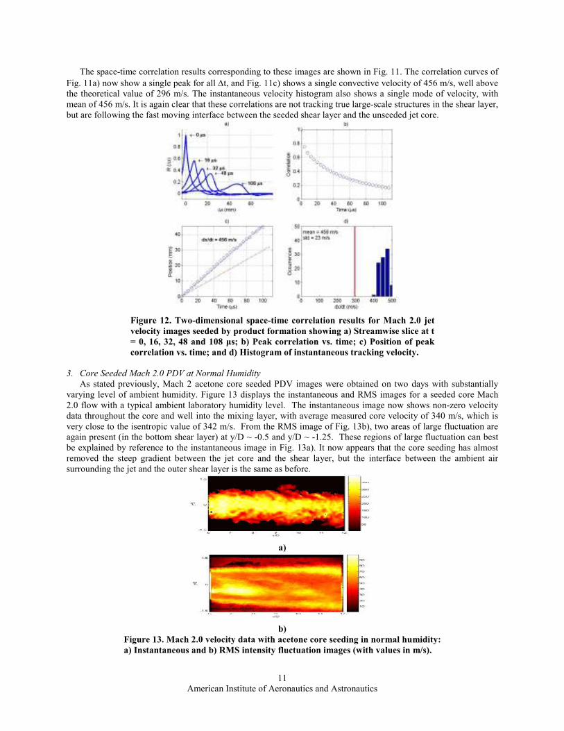
The space-time correlation results corresponding to these images are shown in Fig. 11. The correlation curves of

Fig. 11a) now show a single peak for all ∆t, and Fig. 11c) shows a single convective velocity of 456 m/s, well above the theoretical value of 296 m/s. The instantaneous velocity histogram also shows a single mode of velocity, with

mean of 456 m/s. It is again clear that these correlations are not tracking true large-scale structures in the shear layer,

but are following the fast moving interface between the seeded shear layer and the unseeded jet core.


velocity images seeded by product formation showing a) Streamwise slice at t

= 0, 16, 32, 48 and 108 µs; b) Peak correlation vs. time; c) Position of peak


3. Core Seeded Mach 2.0 PDV at Normal Humidity

As stated previously, Mach 2 acetone core seeded PDV images were obtained on two days with substantially

varying level of ambient humidity. Figure 13 displays the instantaneous and RMS images for a seeded core Mach

2.0 flow with a typical ambient laboratory humidity level. The instantaneous image now shows non-zero velocity

data throughout the core and well into the mixing layer, with average measured core velocity of 340 m/s, which is

very close to the isentropic value of 342 m/s. From the RMS image of Fig. 13b), two areas of large fluctuation are

again present (in the bottom shear layer) at y/D ~ -0.5 and y/D ~ -1.25. These regions of large fluctuation can best

be explained by reference to the instantaneous image in Fig. 13a). It now appears that the core seeding has almost

removed the steep gradient between the jet core and the shear layer, but the interface between the ambient air

surrounding the jet and the outer shear layer is the same as before.

a)

b)

Figure 13. Mach 2.0 velocity data with acetone core seeding in normal humidity:

a) Instantaneous and b) RMS intensity fluctuation images (with values in m/s).


12

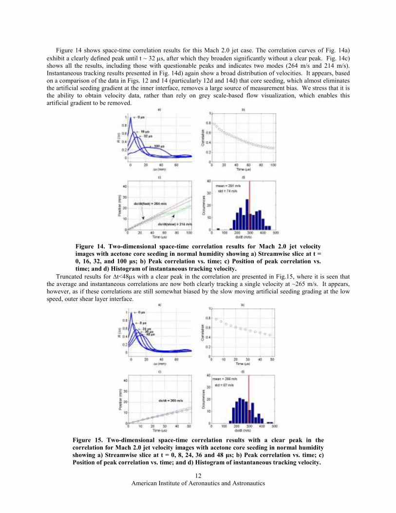
Figure 14 shows space-time correlation results for this Mach 2.0 jet case. The correlation curves of Fig. 14a)

exhibit a clearly defined peak until t ~ 32 µs, after which they broaden significantly without a clear peak. Fig. 14c) shows all the results, including those with questionable peaks and indicates two modes (264 m/s and 214 m/s).

Instantaneous tracking results presented in Fig. 14d) again show a broad distribution of velocities. It appears, based

on a comparison of the data in Figs. 12 and 14 (particularly 12d and 14d) that core seeding, which almost eliminates

the artificial seeding gradient at the inner interface, removes a large source of measurement bias. We stress that it is

the ability to obtain velocity data, rather than rely on grey scale-based flow visualization, which enables this

artificial gradient to be removed.

Figure 14. Two-dimensional space-time correlation results for Mach 2.0 jet velocity

images with acetone core seeding in normal humidity showing a) Streamwise slice at t =

0, 16, 32, and 100 µs; b) Peak correlation vs. time; c) Position of peak correlation vs.

time; and d) Histogram of instantaneous tracking velocity.

Truncated results for ∆t<48µs with a clear peak in the correlation are presented in Fig.15, where it is seen that the average and instantaneous correlations are now both clearly tracking a single velocity at ~265 m/s. It appears,

however, as if these correlations are still somewhat biased by the slow moving artificial seeding grading at the low

speed, outer shear layer interface.

Figure 15. Two-dimensional space-time correlation results with a clear peak in the

correlation for Mach 2.0 jet velocity images with acetone core seeding in normal humidity

showing a) Streamwise slice at t = 0, 8, 24, 36 and 48 µs; b) Peak correlation vs. time; c)

Position of peak correlation vs. time; and d) Histogram of instantaneous tracking velocity.


13

The space-time correlation results in Fig. 15 are similar to those presented by Thurow et al. [2005] for the Mach

2.0 case with acetone core and product formation seeding in normal humidity. In this earlier work, a large outer

shear layer seeding gradient was also evident in PDV images, which also appeared to bias the results toward lower

velocity. This artificial gradient, as discussed in the introduction, was dealt with by arbitrarily extrapolating velocity

values into unseeded regions of the flow field image. After the application of this extrapolation procedure, the

measured convective velocity obtained from space-time correlations matched closely the theoretical convective

velocity. These results suggested that the measurements should be performed again, with effort made to obtain data

as far out into the outer shear layer as possible.

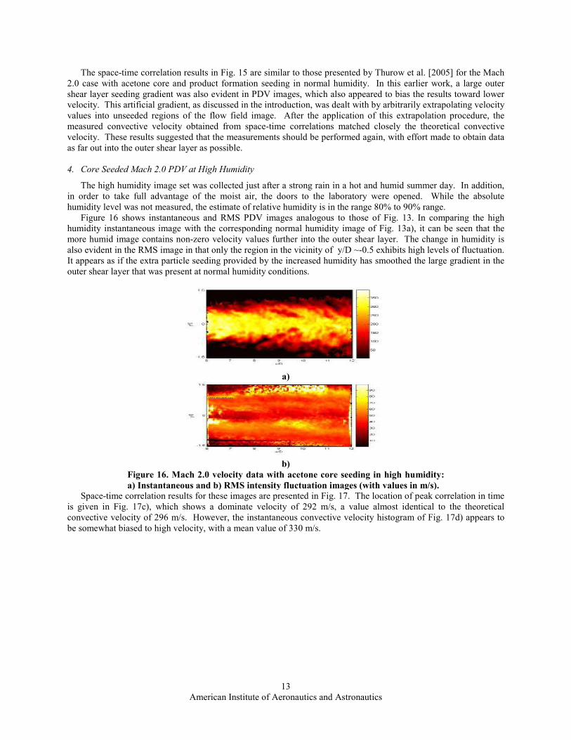
4. Core Seeded Mach 2.0 PDV at High Humidity

The high humidity image set was collected just after a strong rain in a hot and humid summer day. In addition,

in order to take full advantage of the moist air, the doors to the laboratory were opened. While the absolute

humidity level was not measured, the estimate of relative humidity is in the range 80% to 90% range.

Figure 16 shows instantaneous and RMS PDV images analogous to those of Fig. 13. In comparing the high

humidity instantaneous image with the corresponding normal humidity image of Fig. 13a), it can be seen that the

more humid image contains non-zero velocity values further into the outer shear layer. The change in humidity is

also evident in the RMS image in that only the region in the vicinity of y/D ~-0.5 exhibits high levels of fluctuation.

It appears as if the extra particle seeding provided by the increased humidity has smoothed the large gradient in the

outer shear layer that was present at normal humidity conditions.

a)

b)

Figure 16. Mach 2.0 velocity data with acetone core seeding in high humidity:

a) Instantaneous and b) RMS intensity fluctuation images (with values in m/s).

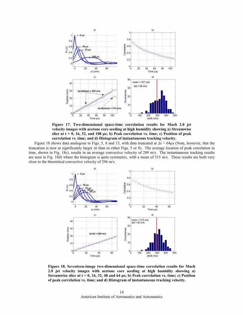
Space-time correlation results for these images are presented in Fig. 17. The location of peak correlation in time

is given in Fig. 17c), which shows a dominate velocity of 292 m/s, a value almost identical to the theoretical

convective velocity of 296 m/s. However, the instantaneous convective velocity histogram of Fig. 17d) appears to

be somewhat biased to high velocity, with a mean value of 330 m/s.


14


velocity images with acetone core seeding at high humidity showing a) Streamwise

slice at t = 0, 16, 32, and 108 µs; b) Peak correlation vs. time; c) Position of peak


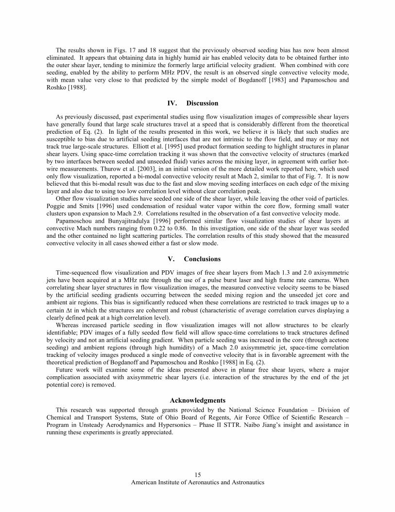
Figure 18 shows data analogous to Figs. 5, 8 and 15, with data truncated at ∆t = 64µs (Note, however, that the

truncation is now at significantly larger ∆t than in either Figs. 5 or 8). The average location of peak correlation in time, shown in Fig. 18c), results in an average convective velocity of 289 m/s. The instantaneous tracking results

are seen in Fig. 18d) where the histogram is quite symmetric, with a mean of 315 m/s. These results are both very

close to the theoretical convective velocity of 296 m/s.

Figure 18. Seventeen-image two-dimensional space-time correlation results for Mach

2.0 jet velocity images with acetone core seeding at high humidity showing a)

Streamwise slice at t = 0, 16, 32, 48 and 64 µs; b) Peak correlation vs. time; c) Position

of peak correlation vs. time; and d) Histogram of instantaneous tracking velocity.


15

The results shown in Figs. 17 and 18 suggest that the previously observed seeding bias has now been almost

eliminated. It appears that obtaining data in highly humid air has enabled velocity data to be obtained further into

the outer shear layer, tending to minimize the formerly large artificial velocity gradient. When combined with core

seeding, enabled by the ability to perform MHz PDV, the result is an observed single convective velocity mode,

with mean value very close to that predicted by the simple model of Bogdanoff [1983] and Papamoschou and

Roshko [1988].

IV. Discussion

As previously discussed, past experimental studies using flow visualization images of compressible shear layers

have generally found that large scale structures travel at a speed that is considerably different from the theoretical

prediction of Eq. (2). In light of the results presented in this work, we believe it is likely that such studies are

susceptible to bias due to artificial seeding interfaces that are not intrinsic to the flow field, and may or may not

track true large-scale structures. Elliott et al. [1995] used product formation seeding to highlight structures in planar

shear layers. Using space-time correlation tracking it was shown that the convective velocity of structures (marked

by two interfaces between seeded and unseeded fluid) varies across the mixing layer, in agreement with earlier hot-

wire measurements. Thurow et al. [2003], in an initial version of the more detailed work reported here, which used

only flow visualization, reported a bi-modal convective velocity result at Mach 2, similar to that of Fig. 7. It is now

believed that this bi-modal result was due to the fast and slow moving seeding interfaces on each edge of the mixing

layer and also due to using too low correlation level without clear correlation peak.

Other flow visualization studies have seeded one side of the shear layer, while leaving the other void of particles.

Poggie and Smits [1996] used condensation of residual water vapor within the core flow, forming small water

clusters upon expansion to Mach 2.9. Correlations resulted in the observation of a fast convective velocity mode.

Papamoschou and Bunyajitradulya [1996] performed similar flow visualization studies of shear layers at

convective Mach numbers ranging from 0.22 to 0.86. In this investigation, one side of the shear layer was seeded

and the other contained no light scattering particles. The correlation results of this study showed that the measured

convective velocity in all cases showed either a fast or slow mode.

V. Conclusions

Time-sequenced flow visualization and PDV images of free shear layers from Mach 1.3 and 2.0 axisymmetric

jets have been acquired at a MHz rate through the use of a pulse burst laser and high frame rate cameras. When

correlating shear layer structures in flow visualization images, the measured convective velocity seems to be biased

by the artificial seeding gradients occurring between the seeded mixing region and the unseeded jet core and

ambient air regions. This bias is significantly reduced when these correlations are restricted to track images up to a

certain ∆t in which the structures are coherent and robust (characteristic of average correlation curves displaying a clearly defined peak at a high correlation level).

Whereas increased particle seeding in flow visualization images will not allow structures to be clearly

identifiable; PDV images of a fully seeded flow field will allow space-time correlations to track structures defined

by velocity and not an artificial seeding gradient. When particle seeding was increased in the core (through acetone

seeding) and ambient regions (through high humidity) of a Mach 2.0 axisymmetric jet, space-time correlation

tracking of velocity images produced a single mode of convective velocity that is in favorable agreement with the

theoretical prediction of Bogdanoff and Papamoschou and Roshko [1988] in Eq. (2).

Future work will examine some of the ideas presented above in planar free shear layers, where a major

complication associated with axisymmetric shear layers (i.e. interaction of the structures by the end of the jet

potential core) is removed.

Acknowledgments

This research was supported through grants provided by the National Science Foundation – Division of

Chemical and Transport Systems, State of Ohio Board of Regents, Air Force Office of Scientific Research –

Program in Unsteady Aerodynamics and Hypersonics – Phase II STTR. Naibo Jiang’s insight and assistance in

running these experiments is greatly appreciated.


16

References

Bogdanoff, D.W., “Compressibility Effects in Turbulent Shear Layers,” AIAA Journal, 21, 1983, pg. 926.

Bourdon, C.J., Dutton, J.C., “Planar Visualizations of Large-Scale Turbulent Structures in Axisymmetric Supersonic

Separated Flows,” Physics of Fluids, 11, 1999, pg. 201.

Brown, G.L., Roshko, A., “On Density Effects and Large Structure in Turbulent Mixing Layers,” Journal of Fluid

Mechanics, 64, 1974, pg. 775.

Clemens, N.T., Mungal, M.G., “Large-scale Structure and Entrainment in the Supersonic Mixing Layer,” Journal of

Fluid Mechanics, 284, 1995, pg. 171.

Elliott, G., Samimy, M., and Arnette, S., “The Characteristics and Evolution of Large-Scale Structures in

Compressible Mixing Layers,” Physics of Fluids, 7, 1995, pg. 864.

Forkey, J.N., “Development and Demonstration of Filtered Rayleigh Scattering – a Laser Based Flow Diagnostic for

Planar Measurements of Velocity, Temperature, and Pressure,” Final TR for NASA Graduate Student Researcher

Fellowship Grant NGT-50826, Princeton University, Princeton, NJ, 1996.

Fourgette, D.C., Mungal, M.G., Dibble, R.W., “Time Evolution of the Shear Layer of a Supersonic Axisymmetric

Jet,” AIAA Journal, 29, 1991, pg. 1123.

Lempert, W., Wu, P., Zhang, B., Miles, R., Lowrance, J., Mastracola, V., and Kosonocky, W., “Pulse-Burst Laser

System for High Speed Flow Diagnostics,” AIAA Paper, 96-0179, 1996.

Mahadevan, R., Guglielmo, J.J., Frank, R.S., Loth, E., “High-Speed Cinematography of Supersonic Mixing Layers,”

AIAA Paper, 1992-3545, 1992.

McGregor, I., “The Vapor Screen Method of Flow Visualization,” Journal of Fluid Mechanics, 11, 1961, pg. 481.

McIntyre, S.S., and Settles, G.S., “Optical Experiments on Axisymmetric Compressible Turbulent Mixing Layers,”

AIAA Paper, 91-0623, 1991.

Papamoschou, D., Roshko, A., “The Compressible Turbulent Shear Layer: An Experimental Study,” Journal of

Fluid Mechanics, 197, 1988, pg. 453.

Papamoschou, D., “Structure of the Compressible Turbulent Shear Layer,” AIAA Paper, 89-0126, 1989.

Papamoschou, D., and Bunyajitradulya, A., “Evolution of Large Eddies in Compressible Shear Layers,” Physics of

Fluids, 9, 1997, pg. 756.

Poggie, J., and Smits, A.J., “Large-Scale Coherent Turbulence Structures in a Compressible Mixing Layer Flow,”

AIAA Paper, 96-0440, 1996.

Samimy, M., Lele, S.K., “Motion of Particles with Inertia in a Compressible Free Shear Layer,” Physics of Fluids, 3,

1991, pg. 1915.

Samimy, M., Zaman, K.B.M.Q., and Reeder, M.F., "Effect of Tabs on the Flow and Noise Field of an Axisymmetric

Jet," AIAA Journal, Vol. 31, pp. 609-619, 1993.

Samimy, M., and Wernet, M., “A Review of Planar Multiple-Component Velocimetry in High Speed Flows,” AIAA

Journal, Vol. 38, No. 4, pp. 553-574, 2000.


17

Samimy, M., Kim, J.-H., Adamovich, I., Utkin, Y., and Kastner, J., “Active Control of High Speed and High

Reynolds Number Free Jet Using Plasma Actuators,” 44th AIAA Aerospace Sciences Meeting and Exhibit, AIAA-

2006-0711, 2006.

Smith, K., Dutton, J., “Evolution and Convection of Large-Scale Structures in Supersonic Reattaching Shear

Flows,” Physics of Fluids, 11, 1999, pg. 2127.

Thurow, B., Samimy, M., Lempert, W., “Compressibility effects on Turbulence Structures of Axisymmetric Mixing

Layers,” Physics of Fluids, 15, 2003, pg. 1755.

Thurow, B., Jaing, N., Samimy, M., Lempert, W., “Narrow-Linewidth Megahertz-Rate Pulse-Burst Laser for High-

Speed Flow Diagnostics,” Applied Optics, 43, 2004, pg. 5064.

Thurow, B., M. Blohm, W.R. Lempert, and M. Samimy, “High Repetition Rate Planar Velocity Measurements in a

Mach 2.0 Compressible Axisymmetric Jet,” AIAA-2005-0515, 43rd AIAA Aerospace Science Meeting, Reno, NV,

Jan 9-12, 2005.

Yip, B., Lyons, K., Long, M., Mungal, M.G., Rarlow, R., and Dibble, R., “Visualization of a Supersonic

Underexpanded Jet by Planar Rayleigh Scattering,” Physics of Fluids, 1, 1989, pg. 1449.

Documents

A Study of Convective Velocity in Supersonic Jets Using ... · American Institute of Aeronautics and Astronautics 2 The last couple of decades have produced many empirical studies