A Structural VAR analysis of the Monetary Policy in Japan · Rt Pt Mt yt t t t t t t t t MR yR MP RP My Ry Py M R P y L M P y a a a a a a a.... c A MP AS LM IS 1 0 0 0 1 1 0 1 0 e

Discussion Paper No. 94

A Structural VAR analysis of the Monetary Policy in Japan

MIHIRA, Tsuyoshi

Economist, Economic Research Institute

SUGIHARA, Shigeru

Ex-Senior Economist, Economic Research Institute

(Senior Economist, Japan Center for Economic Research)

July 2000

Economic Research Institute

Economic Planning Agency

Tokyo, Japan

The views expressed here are the author’s and do not

represent those of the Economic Planning Agency.

A Structural VAR Analysis of the Monetary Policy in Japan

MIHIRA, Tsuyoshi* SUGIHARA, Shigeru

July 2000

Abstract

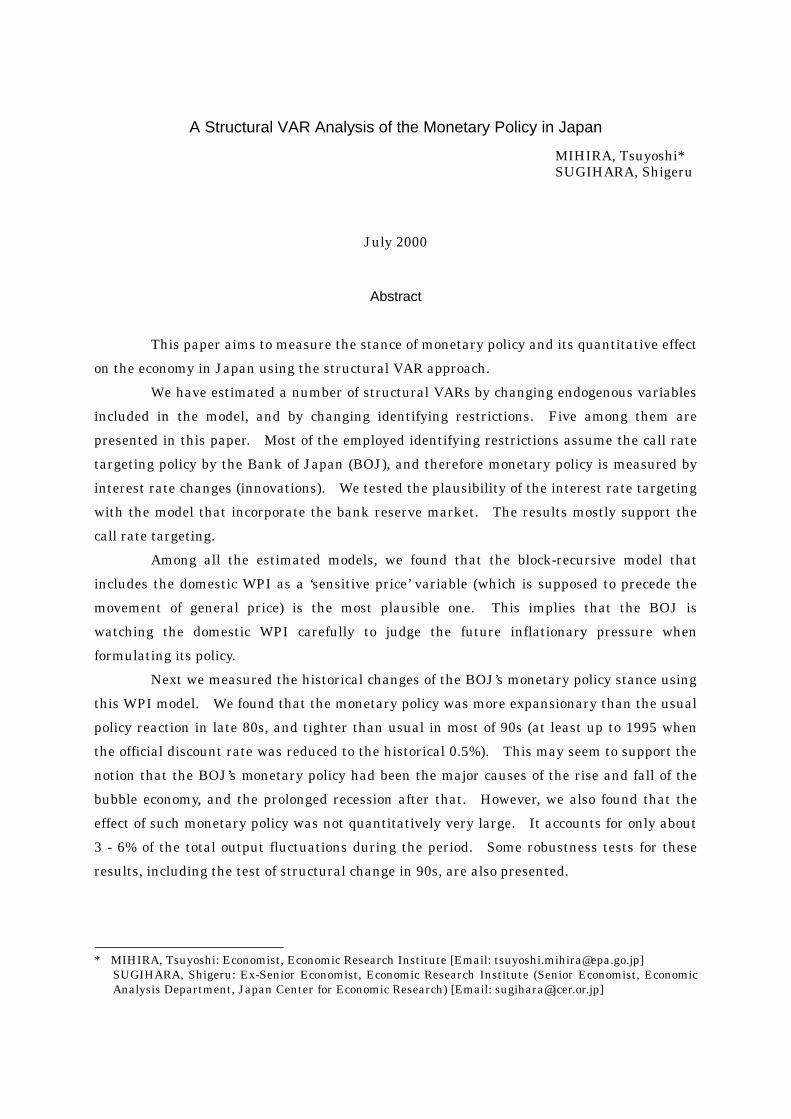
This paper aims to measure the stance of monetary policy and its quantitative effect

on the economy in Japan using the structural VAR approach.

We have estimated a number of structural VARs by changing endogenous variables

included in the model, and by changing identifying restrictions. Five among them are

presented in this paper. Most of the employed identifying restrictions assume the call rate

targeting policy by the Bank of Japan (BOJ), and therefore monetary policy is measured by

interest rate changes (innovations). We tested the plausibility of the interest rate targeting

with the model that incorporate the bank reserve market. The results mostly support the

call rate targeting.

Among all the estimated models, we found that the block-recursive model that

includes the domestic WPI as a ‘sensitive price’ variable (which is supposed to precede the

movement of general price) is the most plausible one. This implies that the BOJ is

watching the domestic WPI carefully to judge the future inflationary pressure when

formulating its policy.

Next we measured the historical changes of the BOJ’s monetary policy stance using

this WPI model. We found that the monetary policy was more expansionary than the usual

policy reaction in late 80s, and tighter than usual in most of 90s (at least up to 1995 when

the official discount rate was reduced to the historical 0.5%). This may seem to support the

notion that the BOJ’s monetary policy had been the major causes of the rise and fall of the

bubble economy, and the prolonged recession after that. However, we also found that the

effect of such monetary policy was not quantitatively very large. It accounts for only about

3 - 6% of the total output fluctuations during the period. Some robustness tests for these

results, including the test of structural change in 90s, are also presented.

* MIHIRA, Tsuyoshi: Economist, Economic Research Institute [Email: [email protected]] SUGIHARA, Shigeru: Ex-Senior Economist, Economic Research Institute (Senior Economist, Economic

Analysis Department, Japan Center for Economic Research) [Email: [email protected]]

- 1 -

A Structural VAR Analysis of the Monetary Policy in Japan1

Introduction

Although most economists would agree that monetary policy affect the economy at

least in the short run, the quantitative degree of it is still in dispute. Moreover, consensus

has not yet achieved even on how we measure the stance of monetary policy of a time. For

example, some argues that the Bank of Japan (BOJ) actually kept monetary policy tight

during the post-bubble recession of early 90s, looking at the very low (sometimes even

negative) growth of monetary aggregates, while the BOJ insists that it kept loosening by

lowering interest rate.

This paper aims to answer these questions of measuring monetary policy stance and

its quantitative effect using the structural VAR approach. The approach is actively used in

the U.S. to deal with these issues, but the application of it to the Japanese data is still

limited2.

The paper is structured as follows. Section 1 briefly explains the structural VAR

approach. Section 2 gives the comparison of estimation results by five different identifying

restrictions, which are based on:

- Four variable aggregate demand - aggregate supply (AD-AS) model {output y, price P,

money stock M, interest rate R }

- Five variable AD-AS model {y, P, M, R, bank reserves RS }

- Block recursive model with sensitive price variable {y, P, M, R, sensitive price Ps }

- Simultaneous model with sensitive price variable {y, P, M, R, Ps }

- Long-run neutrality restrictions {y, P, M, R }

Section 3 analyses the effect of monetary policy and the changes of monetary policy stance in

Japan using the block-recursive model (with the domestic Wholesale Price Index (WPI) used

as a sensitive price variable), which showed the most plausible estimation results in the

Section 2. Comparison with the results by the bank reserve model is also given.

l This Paper is first prepared for the International Workshop on Econometric Modelling held by the

Economic Research Institute, Economic Planning Agency of the Japanese Government; Tokyo, March 2-3, 2000. The authors appreciate the comments by Dr. Miyao, Ryuzo (Kobe University), Dr. Gerald Holtham (Norwich Credit Management), Prof. Stephen Hall (Imperial College), Dr. Raymond J. Barrel (NIESR: National Institute for Economic and Social Research), and Dr. Andrew Levin (Federal Reserve Bord) at the workshop. The authors also thank Prof. Christopher A. Sims, Prof. Ben S. Bernanke, Prof. Mark W. Watson (Princeton University), Dr. Shioji, Etsuro (Yokohama National University), Dr. Kenneth Kasa (Federal Reserve Bank of San Francisco), Prof. Michael M. Hutchison, Dr. Yin-Wong Cheung (University of California Santa Cruz) for the suggestions on the research. Authors are responsible for all the errors and mistakes.

2 Major exceptions are Shioji (2000), Miyao (1999a, 1999b), Kasa and Popper (1997), Hutchinson (1994), West (1993), and Iwabuchi (1990).

- 2 -

1. Structural VAR Approach

An ordinary VAR (vector auto-regression) model describes the dynamic movements

of endogenous variables by their own past values. It is expressed as:

;221t1 tqtqtt x uBxBxBkx +++++= −−− K tu ~ 0,... (dii ∑ )u [1]

ttL uxBk ++= )(

where tx is a vector of endogenous variables, k is a vector of constants, B’s are matrices of

coefficients, tu is a vector of disturbances, and L is the lag operator.

This is a very generalised model, which imposes no restriction on the form of B(L ),

i.e. the dynamic relationship among variables. It is known that VAR models are

particularly useful for forecasting.

One weakness of such a VAR as a tool of economic analysis is, however, that each

equation has no economic interpretation. This causes a problem for our purpose of

analysing monetary policy effect, as we cannot tell what is the ‘monetary policy’ in a VAR.

Consider a VAR model with four endogenous variables for example: output (y ),

price (P ), interest rate (R ), and money stock (M ). One may attempt to analyse the effect of

an interest rate raising monetary policy by looking at the impulse responses to the

innovations in the R equation ( Ru ). But the R equation may reflect not only monetary

policy reaction to the economy but also money demand and other economic relations.

Accordingly, its innovation Ru will contain not only the innovations in monetary policy but

also the money demand and other kinds of shocks. Thus naively interpreting the impulse

responses to Ru as the effect of monetary policy may be problematic. We need to ‘identify’

the underlying ‘structure’ of the economy reflected in the VAR, in particular that of monetary

policy reaction and its innovation, to measure the true monetary policy effect.

This is what the ‘Structural VAR’ approach intends to do. A structural VAR is

expressed as:

[2] ;)(0 ttt L ε++= xAcxA tε ~ i.i.d.(0, D )

The structure of simultaneous determination in the economy is now explicitly

represented in the matrix A0. Each equation is assumed to represent a specific economic

relation such as monetary policy reaction or money demand, and thus the innovation ε

represents the exogenous shocks in it. Since we assume ε’s are exogenous shocks, they are

orthogonal to each other; i.e. the variance matrix D is a diagonal matrix by assumption.

From the viewpoint of a structural VAR, an ordinary VAR [1] can be regarded as the

reduced form of [2]. Multiplying the both side of [2] by 10−A :

ttt L ε10

10

10 )( −−− ++= AxAAcAx

ttL uxBk ++= )(

- 3 -

Accordingly, the relationship between the structural and the reduced form parameters are:

[3-1] )()( 00 LL BAAk,Ac ==

[3-2] =′⇔= −− )( 10

100 ADAuA tt ε ∑u

The problem of estimating the structural VAR [2] is that it is a system of

simultaneous equations and thus the OLS estimator will be biased and inconsistent. A

usual procedure is to estimate the reduced form VAR [1] by OLS, and recover the structural

parameters using the relationship [3-1,2]. If A0 is estimated, other structural parameters

can be recovered by [3-1]. A0 (together with D) is to be recovered using [3-2]. But while A0

and D contain n2 unknown parameters, ∑u has only n(n+1)/2 information in it as it is a

symmetric matrix. Therefore l ≥ n(n-1)/2 additional restrictions are required for the

identification of A0.

We examine five different identifying restrictions for the Japanese economy in the

next section.

- 4 -

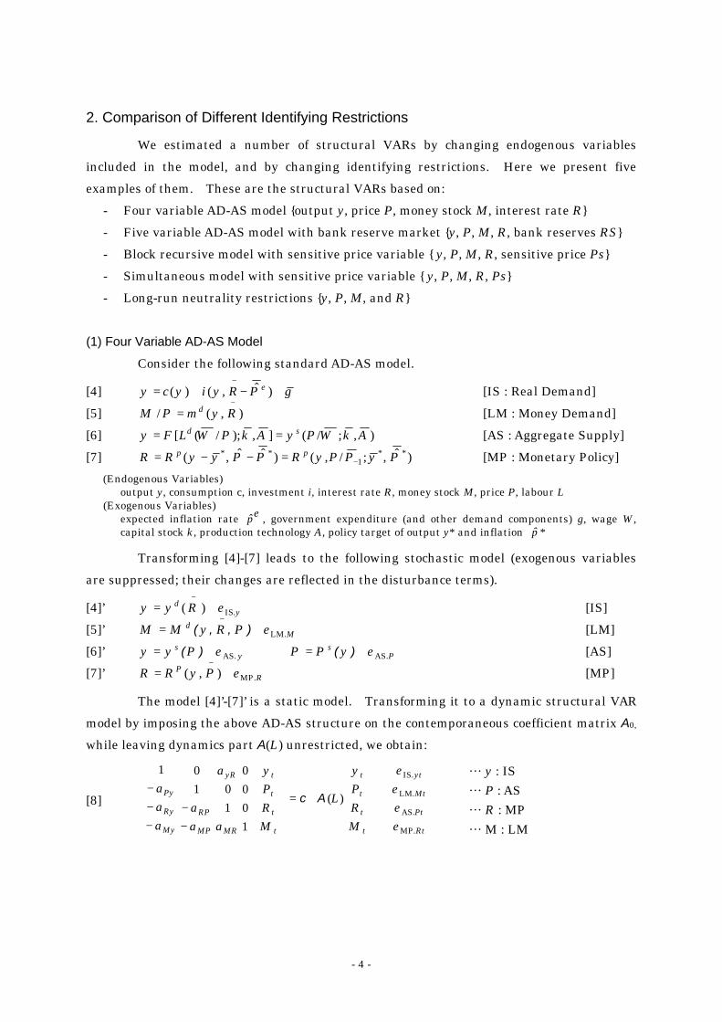
2. Comparison of Different Identifying Restrictions

We estimated a number of structural VARs by changing endogenous variables

included in the model, and by changing identifying restrictions. Here we present five

examples of them. These are the structural VARs based on:

- Four variable AD-AS model {output y, price P, money stock M, interest rate R}

- Five variable AD-AS model with bank reserve market {y, P, M, R, bank reserves RS}

- Block recursive model with sensitive price variable { y, P, M, R, sensitive price Ps}

- Simultaneous model with sensitive price variable { y, P, M, R, Ps}

- Long-run neutrality restrictions {y, P, M, and R}

(1) Four Variable AD-AS Model

Consider the following standard AD-AS model.

[4] gPRyiycy e +−+=−++

)ˆ,()( [IS : Real Demand]

[5] ),(/−+

= RymPM d [LM : Money Demand]

[6] ),;/(],);/([ AkWPyAkPWLFy sd+

== [AS : Aggregate Supply]

[7] )ˆ,;/,()ˆˆ,( 1∗∗

−

++∗∗ =−−= PyPPyRPPyyRR pp [MP : Monetary Policy]

(Endogenous Variables) output y, consumption c, investment i, interest rate R, money stock M, price P, labour L

(Exogenous Variables) expected inflation rate ep , government expenditure (and other demand components) g, wage W, capital stock k, production technology A, policy target of output y* and inflation *p

Transforming [4]-[7] leads to the following stochastic model (exogenous variables

are suppressed; their changes are reflected in the disturbance terms).

[4]’ .yd Ryy IS)( ε+=

− [IS]

[5]’ Md PRyMM .),,( LMε+=

+−+ [LM]

[6]’ Ps

ys yPPPyy .. )()( ASAS εε +=⇔+=

++ [AS]

[7]’ RP PyRR .MP),( ε+=

−+ [MP]

The model [4]’-[7]’ is a static model. Transforming it to a dynamic structural VAR

model by imposing the above AD-AS structure on the contemporaneous coefficient matrix A0,

while leaving dynamics part A(L) unrestricted, we obtain:

… y : IS … P : AS … R : MP

[8]

+

+=

−−

−−−

Rt

Pt

Mt

yt

t

t

t

t

t

t

t

t

MR

yR

MP

RP

My

Ry

Py

MRPy

L

MRPy

a

a

aa

aaa

.

.

.

.

Ac

MP

AS

LM

IS

)(

1000

101

01

εεεε

… M : LM

- 5 -

The equation [8] suggests five zero restrictions on A0. We further assume the

investment decision lag (i.e., 0=yRa ), as six restrictions are required for identification.

Thus the model results in a recursive VAR (no simultaneous determination in the system: A0

reduces to a lower triangular matrix and usual Choleski factorisation is applicable). If the

assumed AD-AS structure is identified correctly by such recursive restrictions, the estimated

A0 matrix should have the signs indicated by [8].

Also, the estimated impulse responses are expected to show the response patterns

indicated by the equation [9] below, which is obtained by the comparative statics of [4]’-[7]’.

[9]

+−+−−

++−

+++

=

.M

P.R

S.P

.y

dddd

dMdRdPdy

LM

M

A

IS

000

?? εεεε

- Positive real demand (lS) shock ( 0IS >yd .ε ) will increase y, P, and R

- Negative supply (AS) shock ( 0AS >Pd .ε ) will decrease y, and raise P and R

- Tight monetary (MP) shock ( 0MP >Rd .ε ) will decrease y, P, M, while raising R

- Money demand (LM) shock ( 0LM >Md .ε ) will just increase M, and will not affect y, P, and R

We estimated the structural VAR [8] using quarterly data (y: log of real GDP, P : log

of GDP deflator, R: call money rate, M: log of M2+CD) from 1980Q1 to 1999Q43. We

examined ten different specifications of data forms (differenced or in levels, seasonally

adjusted or not adjusted) and lag length (two lags or four lags). The results have some

unfavourable features, however.

Table 1 shows the estimated A0 matrices. Although the monetary policy reaction

function [MP equation] is estimated with correct signs, the signs of the AS and LM equations

tend to go against the supposed model (the ‘wrong’ signs are marked by shadings). The

estimated AS curves are all negatively sloped in the contemporaneous y-P plane, which is

more plausible for AD curves. The estimated LM equations tend to show negative

contemporaneous relations with y and P, and a positive relation with R; this may suggest

that some part of monetary authority’s policy reaction is reflected in the estimated LM

equations (i.e., BOJ’s behaviour is not fully grasped by the estimated MP equations).

The estimated impulse responses also show some unexpected patterns. Figure 1 shows

examples of them4. Most notably, P goes up after a tight monetary policy (MP) shock. This is a

3 We also estimated the structural VAR [8] and all other models presented in this paper with monthly data,

using industrial production instead of real GDP, and consumer price index instead of GDP deflator. The results are similar to those of quarterly data estimation.

4 We take the four period differenced models for examples, as they are clear to see without noisy fluctuations. One example each is selected for the two specifications of interest rate [differenced or in level], choosing lag length by Akaike Information Criteria. The examples of latter part of the paper are selected in the same way.

- 6 -

phenomenon known as the “price puzzle”, which frequently appears in structural VAR

analysis in particular when monetary policy is measured by interest rate. The price puzzle

is a common feature in all the ten specifications estimated here.

Another common puzzling result is that y and P respond positively to a increased

money demand (LM) shock. This reinforces our suspect that the estimated LM equation

may reflect BOJ’s policy reaction in some part.

Other unfavourable features of the impulse responses are:

- Price P initially responds negatively to a positive IS shock in all specifications (though

this response is not strong and short-lived)

- Negatives AS shock causes interest rate fall in some specifications. There are also

cases in which a negative AS shock leads to output increase.

Table 1: Contemporaneous Coefficient Matrices of the Four Variable AD-AS Model

Log-Difference (1) [R: Level] 2 Lags Log-Difference (1) [R: Level] 4 Lags

1.0000 0.0000 0.0000 0.0000 1.0000 0.0000 0.0000 0.0000 0.0870 1.0000 0.0000 0.0000 0.1011 1.0000 0.0000 0.0000 -0.0822 -0.4094* 1.0000 0.0000 -0.0963 -0.4439* 1.0000 0.0000 0.0591 -0.0168 -0.1245 1.0000 0.0377 0.0295 -0.1530 1.0000

Log-Difference (1) [R: Difference] 2 Lags Log-Difference (1) [R: Difference] 4 Lags

1.0000 0.0000 0.0000 0.0000 1.0000 0.0000 0.0000 0.0000 0.1090 1.0000 0.0000 0.0000 0.0769 1.0000 0.0000 0.0000 -0.0974 -0.2404 1.0000 0.0000 -0.0537 -0.2947* 1.0000 0.0000 0.0589 0.0346 -0.1439 1.0000 0.0638 0.1262 -0.2030* 1.0000


1.0000 0.0000 0.0000 0.0000 1.0000 0.0000 0.0000 0.0000 0.1451* 1.0000 0.0000 0.0000 0.1029 1.0000 0.0000 0.0000 -0.1159* -0.1676 1.0000 0.0000 -0.1301* -0.2333* 1.0000 0.0000 0.0982 0.0131 -0.1678 1.0000 0.0934 0.0610 -0.2790* 1.0000


1.0000 0.0000 0.0000 0.0000 1.0000 0.0000 0.0000 0.0000 0.1234* 1.0000 0.0000 0.0000 0.0857 1.0000 0.0000 0.0000 -0.0738 -0.2412 1.0000 0.0000 -0.0040 -0.2734 1.0000 0.0000 0.1124 0.0702 -0.1503 1.0000 0.0962 0.1544 -0.2248* 1.0000

Log-Level [R: Level] 2 Lags LogLevel [R: Level] 4 Lags

1.0000 0.0000 0.0000 0.0000 1.0000 0.0000 0.0000 0.0000 0.0475 1.0000 0.0000 0.0000 0.0535 1.0000 0.0000 0.0000 -0.1072 -0.3382* 1.0000 0.0000 -0.0981 -0.3765* 1.0000 0.0000 0.0424 -0.0453 -0.1096 1.0000 0.0079 0.0580 -0.1270 1.0000

Log-Difference (1): variables are log-differenced from the previous period, SA (except R)

Log-Difference (4): variables are log-differenced from the same period of the previous year, not SA (except R)

Log-Level: variables are in logs, SA (except R)

Unexpected signs of coefficients are marked by shadings

Coefficients of significance at 2 s.e. are marked by *

- 7 -

Figure 1: Impulse Responses of the Four Variable AD-AS structural VAR

(1) Log-Difference (4) [R: Level] 4 Lags

(2) Log-Difference (4) [R: Difference] 2 Lags

- 8 -

(2) Bank Reserve Model

The reason why we obtained the results with some unpleasant features in the

previous section may be because the model was too simple and therefore ignored some

important transmission pass of monetary policy. In this regard, we built up several

extended models, each of which contains an additional transmission variable, and estimated

corresponding structural VARs. The variables added are: long-term interest rate, exchange

rate, stock price, bank loans, high-powered money, and bank reserves. The results did not

improve much however: the price puzzle still remains; y and P continues to respond

positively to a money demand (LM) shock.

Here we show the example of the bank reserve model. A unique feature of the

model is that it can cope with the question of a particular interest: what is the policy

variable of the BOJ?

So far we have assumed the interest rate (the call rate) targeting policy by the BOJ,

in which the BOJ controls the short term call rate as a sole policy variable (as reflected in

the specification of the policy reaction function [7]’). This is in accordance with what the

BOJ says.

However, this might be an extreme assumption. The complete interest rate

targeting implies a larger fluctuation of monetary aggregates, as the fluctuation of money

demand would be fully accommodated by the supply of money by the authority, to suppress

the changes of interest rate. If the central bank considers the stability in monetary

aggregates also desirable, however, the bank may not fully accommodate the fluctuating

money demand. In this case, monetary aggregates cared by the bank also constitute a part of

the bank’s policy variables, and the bank’s policy stance will not be fully captured by a single

variable of interest rate innovations. In the case of complete monetary aggregate target (an

opposite extreme case), the innovations in interest rate will not contain the information of

monetary policy at all, but just reflect the changes in money demand or other shocks. Thus,

assuming interest rate targeting a priori might be problematic. It might be better to consider

the possibility that the BOJ cares both of interest rate and monetary aggregates.

Bank reserves would be one of the natural candidates for such monetary quantity

cared by the central bank, as the reserve market is where the actual monetary policy

operations take place.

We specify the structure of the reserve market as follows.

[10] .RP RS ,P ,yRR MP)( ε+=

+++ [MP: Monetary Policy]

[11] .RSd M ,RRSRS RD)( ε+=

+− [RD: Reserve Demand]

The reserve (RS) supply curve by the policy authority is assumed to be positively sloped

in the R-RS plane, reflecting the assumption that the central bank would avoid large volatility of

both of interest rate and bank reserves. The slope of the curve becomes flatter if the

- 9 -

authority behaves more like interest rate targeting way, and becomes sharper as the

authority cares more about the reserve quantity. The reserve demand curve is supposed to

be negatively sloped in the R-RS plane, and it is assumed that, at least in a very short run,

only M (large part of which is bank deposit) affects the curve through reserve requirement.

The corresponding structural VAR is:

… y : IS … P : AS … R : MP … M : LM

[12]

+

+=

−−−

−−−−

RSt

Mt

Rt

Pt

yt

t

t

t

t

t

t

t

t

t

t

S.MRRS.R

MRMPMy

R.RSRPRy

Py

yR

RMRPy

L

RMRPy

aaaaa

aaaa

a

.

.

.

.

.

Ac

RD

LM

MP

AS

IS

S

)(

S10001

0100010001

εεεεε

… RS : RD

This is a just-identified model. The structural monetary policy shock is now a

mixture of the interest rate innovation and the reserve innovation of the reduced form VAR,

with the weight of the slope of policy reaction curve in the reserve market, aR.RS•

[13] PtRPytRyRstR.RsRtRt uauauau −−−=.MPε (Remember [3-2] tt uA0=ε )

Note that the structural VAR [12] nests the interest rate targeting policy, in which

case 0=R.RSa . Thus we could test the interest rate targeting by examining the

significance of the estimated coefficient.

However, the estimation did not proceed well: the RATS @Bernanke procedure

somehow failed to achieve convergence in maximum likelihood iteration in four of ten

specifications. This may be suggesting that the identifying restrictions to distinguish the

monetary policy and the reserve demand (MP does not respond to current M, and RD does

not respond to current y and P ) are too weak.

Nevertheless, as presented in the Table 2-(1), the coefficient R.RSa is estimated as

exactly zero (at least down to four places of disimals) in four of the converged six

spesifications, thus suggesting the BOJ’s policy is actually the interest rate targeting policy.

aR.RS is significantly different from zero only in one specification.

An alternative strategy to test the interest rate targeting is to impose 0=R.RSa as

an additional identifying restriction on [12], and to test the over-identification. The same

strategy can be applied to test the reserve target policy. Specifying the monetary policy

equation under reserve targeting as:

[14] RSP P ,yRS RS MP.)( ε+=

−− [MP(RS)]

And the over-identifying reserve targeting structural VAR is:

- 10 -

… y : IS … P : AS … R : RD … M : LM

[15]

+

+=

−−−

−

RSt

Mt

Rt

Pt

yt

t

t

t

t

t

t

t

t

t

t

RS.PRS.y

MRMPMy

R.RSRM

Py

yR

RM

RPy

L

RM

RPy

aaaaa

aaa

a

.

.

.

.

.

Ac

MP

LM

RD

AS

IS

S

)(

S10001

10000010001

εεεεε

… RS : MP

The estimated coefficient matrices and the results of over-identification tests are

given in Table 2-(2) and (3). The results are in favour of the call rate targeting (as one

might expect). With the call rate target model, over-identifying restriction is not rejected in

nine specifications out of ten at 5% significance level. All the coefficients of MP and RD

equations are signed correctly. On the other hand, the reserve target model is rejected by

the over-identification test in eight of the nine specifications estimated (convergence was not

achieved in one specification). The estimated MP and RD equations tend to have wrong

signs5.

Examples of estimated impulse responses for each model are shown in Figure 2-1

and 2-2. The interest rate target model shows similar responses to those in the previous

section: the price puzzle is still present, and LM shock causes output and price rise. The

impulse responses of the reserve target model are also accompanied by some unfavourable

features. They are:

- Interest rate R rises after a loosening MP shock (increased reserve supply shock) in five

specifications out of nine. This is known as the “liquidity puzzle”, which often occurs

especially when some kind of monetary quantity is specified as a policy variable.

- Output y and price P declines after a loosening MP shock in some specification.

- Price P goes up in response to an increased reserve demand shock in every specification.

5 The conclusion that the call rate target is more plausible is also obtained by the monthly data estimation.

With monthly data, the nested model is successfully converged in seven specifications and in all of them the coefficient aR.RS is estimated as exactly zero (at least down to four places of decimals); all other coefficients of the MP and RD equations are signed correctly except one case where aRy is insignificantly negative. The call rate target model achieved convergence in all the ten specifications, and none of them is rejected by the over-identification test; the MP and RD coefficients are signed correctly in most cases although in some specifications aRy is estimated insignificantly negative. The reserve target model fails to achieve convergence in five specifications, and three of the rest are rejected by the over-identification test; the MP equation has wrong signs in all of the five converged specifications.

- 11 -

Table 2: Contemporaneous Coefficient Matrices of the Bank Reserve Model (Results of Over-Identification Test Attached Where Applied)

(1) Nested Model


Convergence Not Achieved Convergence Not Achieved


1.0000 0.0000 -0.0277 0.0000 0.0000 1.0000 0.0000 0.0852 0.0000 0.0000 0.1097 1.0000 0.0000 0.0000 0.0000 0.0966 1.0000 0.0000 0.0000 0.0000 -0.0842 -0.2493 1.0000 0.0000 0.0000 -0.1132 -0.3375* 1.0000 0.0000 -0.0000 0.0607 0.0169 -0.1448 1.0000 0.0000 0.0758 0.1466 -0.2253* 1.0000 0.0000 0.0000 0.0000 0.5918 -1.3868* 1.0000 0.0000 0.0000 0.6857 -1.6138* 1.0000


Convergence Not Achieved Convergence Not Achieved


1.0000 0.0000 -3.8446* 0.0000 0.0000 1.0000 0.0000 1.2383 0.0000 0.0000 -0.0881 1.0000 0.0000 0.0000 0.0000 -0.0405 1.0000 0.0000 0.0000 0.0000 -2.4833* 1.9450* 1.0000 0.0000 0.9733* -0.7996 -0.7999 1.0000 0.0000 -0.0277 -0.6042 -0.4718* -0.3172* 1.0000 0.0000 0.0750 0.1322 -0.2180* 1.0000 0.0000 0.0000 0.0000 0.3372 -4.2227 1.0000 0.0000 0.0000 1.0654* -1.3553* 1.0000

Log-Level [R: Level] 2 Lags Log-Level [R: Level] 4 Lags

1.0000 0.0000 0.3752 0.0000 0.0000 1.0000 0.0000 0.5664 0.0000 0.0000 0.0256 1.0000 0.0000 0.0000 0.0000 0.0216 1.0000 0.0000 0.0000 0.0000 -0.2359 -0.3045 1.0000 0.0000 -0.0000 -0.3294 -0.3367 1.0000 0.0000 -0.0000 0.0504 -0.0612 -0.0233 1.0000 0.0000 0.0181 -0.0175 -0.0359 1.0000 0.0000 0.0000 0.0000 0.1651 -1.4856* 1.0000 0.0000 0.0000 0.3249 -1.6338* 1.0000

- 12 -

Table 2: Contemporaneous Coefficient Matrices of the Bank Reserve Model (Continued) (Results of Over-Identification Test Attached Where Applied)

(2) Call Rate Target Model Log-Difference (1) [R: Level] 2 Lags Log-Difference (1) [R: Level] 4 Lags

1.0000 0.0000 -0.0004 0.0000 0.0000 1.0000 0.0000 -0.0002 0.0000 0.0000 0.0867 1.0000 0.0000 0.0000 0.0000 0.1182 1.0000 0.0000 0.0000 0.0000 -0.0837 -0.4181 1.0000 0.0000 0.0000 -0.0975 -0.4567 1.0000 0.0000 0.0000 0.0620 -0.0185 -0.1321 1.0000 0.0000 0.0565 0.0765 -0.1791* 1.0000 0.0000 0.0000 0.0000 0.7450 -1.3174* 1.0000 0.0000 0.0000 0.8299* -1.3756* 1.0000 LR Test of Overidentification Chi-Square (1) = 1.91912 Signif. Level = 0.1659534

LR Test of Overidentification Chi-Square (1) = 3.04061 Signif. Level = 0.0812055


1.0000 0.0000 -0.0012 0.0000 0.0000 1.0000 0.0000 -0.0000 0.0000 0.0000 0.1076 1.0000 0.0000 0.0000 0.0000 0.1052 1.0000 0.0000 0.0000 0.0000 -0.0981 -0.2492 1.0000 0.0000 0.0000 -0.0613 -0.3360* 1.0000 0.0000 0.0000 0.0607 0.0169 -0.1448 1.0000 0.0000 0.0758 0.1466 -0.2253* 1.0000 0.0000 0.0000 0.0000 0.5918 -1.3868* 1.0000 0.0000 0.0000 0.6857* -1.6138* 1.0000 LR Test of Overidentification Chi-Square (1) = 0.90324 Signif. Level = 0.3419145



1.0000 0.0000 -0.0093 0.0000 0.0000 1.0000 0.0000 -0.0165 0.0000 0.0000 0.1437 1.0000 0.0000 0.0000 0.0000 0.1183 1.0000 0.0000 0.0000 0.0000 -0.1141 -0.1526 1.0000 0.0000 0.0000 -0.1442 -0.2539 1.0000 0.0000 0.0000 0.0973 -0.0339 -0.1946 1.0000 0.0000 0.0968 0.0516 -0.3410* 1.0000 0.0000 0.0000 0.0000 0.9380 -1.0834* 1.0000 0.0000 0.0000 0.9664 -1.2892* 1.0000 LR Test of Overidentification Chi-Square (1) = 0.04316 Signif. Level = 0.8354190



1.0000 0.0000 -0.0004 0.0000 0.0000 1.0000 0.0000 -0.0000 0.0000 0.0000 0.1338 1.0000 0.0000 0.0000 0.0000 0.1197 1.0000 0.0000 0.0000 0.0000 -0.0847 -0.2618 1.0000 0.0000 0.0000 -0.0696 -0.4460* 1.0000 0.0000 0.0000 0.0911 -0.0146 -0.1413 1.0000 0.0000 0.0868 0.1443 -0.2332* 1.0000 0.0000 0.0000 0.0000 0.7305 -1.3255* 1.0000 0.0000 0.0000 0.9559* -1.3742* 1.0000 LR Test of Overidentification Chi-Square (1) = 1.18973 Signif. Level = 0.2753831


Log-Level (1) [R: Level] 2 Lags Log-Level (1) [R: Level] 4 Lags

1.0000 0.0000 -0.0013 0.0000 0.0000 1.0000 0.0000 -0.0006 0.0000 0.0000 0.0513 1.0000 0.0000 0.0000 0.0000 0.0659 1.0000 0.0000 0.0000 0.0000 -0.0790 -0.2881 1.0000 0.0000 0.0000 -0.0718 -0.2954 1.0000 0.0000 0.0000 0.0504 -0.0612 -0.0233 1.0000 0.0000 0.0181 -0.0175 -0.0359 1.0000 0.0000 0.0000 0.0000 0.1651 -1.4856* 1.0000 0.0000 0.0000 0.3249 -1.6338* 1.0000 LR Test of Overidentification Chi-Square (1) = 1.61416 Signif. Level = 0.2039083


- 13 -

Table 2: Contemporaneous Coefficient Matrices of the Bank Reserve Model (Continued) (Results of Over-Identification Test Attached Where Applied)

(3) Reserve Target Model Log-Difference (1) [R: Level] 2 Lags Log-Difference (1) [R: Level] 4 Lags

1.0000 0.0000 -0.0349 0.0000 0.0000 1.0000 0.0000 -0.0306 0.0000 0.0000 0.0869 1.0000 0.0000 0.0000 0.0000 0.1183* 1.0000 0.0000 0.0000 0.0000 0.0000 0.0000 1.0000 0.3851 0.0203 0.0000 0.0000 1.0000 0.2322 0.0349 0.0792 0.0887 -0.3885 1.0000 0.0000 0.0681 0.1421 -0.3228 1.0000 0.0000 0.2630 -0.4101 0.0000 0.0000 1.0000 0.3935 -0.2826 0.0000 0.0000 1.0000 LR Test of Overidentification Chi-Square (1) = 16.20111 Signif. Level = 0.0000570



1.0000 0.0000 -0.0947 0.0000 0.0000 1.0000 0.0000 -0.0166 0.0000 0.0000 0.1080 1.0000 0.0000 0.0000 0.0000 0.1052 1.0000 0.0000 0.0000 0.0000 0.0000 0.0000 1.0000 0.2938 0.0103 0.0000 0.0000 1.0000 0.0394 0.0267 0.0697 0.0629 -0.3292 1.0000 0.0000 0.0770 0.1544 -0.2486 1.0000 0.0000 0.3400 -0.0531 0.0000 0.0000 1.0000 0.4941 0.0511 0.0000 0.0000 1.0000 LR Test of Overidentification Chi-Square (1) = 11.43414 Signif. Level = 0.0007211



1.0000 0.0000 -0.3247 0.0000 0.0000 0.1180* 1.0000 0.0000 0.0000 0.0000 0.0000 0.0000 1.0000 0.1346 0.0115 0.1068 0.1013 -0.5366 1.0000 0.0000 0.3113 -0.3079 0.0000 0.0000 1.0000

Convergence Not Achieved



1.0000 0.0000 -0.5097 0.0000 0.0000 1.0000 0.0000 0.0291 0.0000 0.0000 0.1708* 1.0000 0.0000 0.0000 0.0000 0.1192 1.0000 0.0000 0.0000 0.0000 0.0000 0.0000 1.0000 -2.1340 0.1851 0.0000 0.0000 1.0000 0.2906 0.0446 0.4791 -0.5978 1.8049 1.0000 0.0000 0.1045 0.2353* -0.4372 1.0000 0.0000 0.2335 0.6668 0.0000 0.0000 1.0000 0.3975 0.0477 0.0000 0.0000 1.0000 LR Test of Overidentification Chi-Square (1) = 0.04496 Signif. Level = 0.8320748


Log-Level (1) [R: Level] 2 Lags Log-Level (1) [R: Level] 4 Lags

1.0000 0.0000 -0.1291 0.0000 0.0000 1.0000 0.0000 -0.0979 0.0000 0.0000 0.0512 1.0000 0.0000 0.0000 0.0000 0.0659 1.0000 0.0000 0.0000 0.0000 0.0000 0.0000 1.0000 0.1511 -0.0046 0.0000 0.0000 1.0000 0.1774 0.0029 0.0530 -0.0295 -0.1333 1.0000 0.0000 0.0214 0.0191 -0.1597 1.0000 0.0000 0.2477 -0.6126 0.0000 0.0000 1.0000 0.2859 -0.9770 0.0000 0.0000 1.0000 LR Test of Overidentification Chi-Square (1) = 12.70265 Signif. Level = 0.0003651


Log-Difference (1): variables are log-differenced from the previous period, SA (except R) Log-Difference (4): variables are log-differenced from the same period of the previous year, not SA (except R) Log-Level: variables are in logs, SA (except R) Unexpected signs of coefficients are marked by shadings Coefficients of significance at 2 s.e. are marked by*

- 14 -

Figure 2-1: Impulse Responses of the Bank Reserve Model [Call Rate Target]



- 15 -

Figure 2-2: Impulse Responses of the Bank Reserve Model [Reserve Target]



- 16 -

(3) Block-Recursive Model with Sensitive Price Variable

A widely adopted practice to cope with the price puzzle is to include a ‘sensitive

price’ variable Ps (which is supposed to precede the movement of general prices) in the

structural VAR, and assume that monetary authority react to such a sensitive price

contemporaneously. Thus the monetary policy reaction function in the VAR is now:

[16] ,,;Ps ,P ,yRR Rtq-t1-ttttPtt .xx MP)( ε+= K

or

[17] tPsRtRPtRyRt PsaPayacR ,+++= 1Ra+ ’ 21 Rt ax +− ’ 2−tx Rna++ K ’ Rtqt .x MPε+−

where tx is a vector of endogenous variables.

The reason why such a specification solves the price puzzle can be considered as

follows. Suppose we estimate the policy reaction by [17]’ below, which does not include the

current value of tPs in the information set of the authority, when the true policy reaction is

described by [17].

[17]’ tRPtRyRt PayacR ++= 1Ra+ ’ 21 Rt ax +− ’ 2−tx Rna++ K ’ Rtqt .x MPε+−

Then the resulting estimated exogenous policy shock +Rt.ˆMPε will include the actually

endogenous reaction of the authority to the part of tPs that is orthogonal to Pt, i.e. Ps.tε : the

residual of regressing Ps by P. If we regress +Rt.ˆMPε by Ps.tε , then:

RtPstR.PsRt a .. ˆˆˆˆ MPMP εεε +=+ R.SPa : estimator of coefficient on tPs in [17]

Rt.ˆMPε : estimator of true policy shock by [17]

The first term of the RHS is the actually endogenous policy reaction to Pstε and the second

term is the truely exogenous policy shock. The wrongly estimated impulse response of the

general price P to a policy shock thus will be:

.Rt.Rt

stPs.tR.Ps

Ps.t

stRt

Rt

stst d

Pda

Pd

PdP MP

MPMP

MP

εε

εε

εε

ˆˆ

ˆˆˆ

ˆˆ

.. ∂

∂+

∂∂

=∂∂

= ++++

++

Thus, if Ps precedes the movement of the general price P ( 0/ >∂∂ + Ps.tstP ε ), and if the policy

authority reacts to the rise of Ps by raising interest rate R ( 0>R.Psa ), then one might result

in finding positive response of P to a tight monetary policy shock, even if the true response is

negative ( 0/ MP <∂∂ + .RtstP ε ).

Christiano, Eichembaum and Evans (1998) estimate a block-recursive structural VAR

with such a sensitive price variable. A great merit of a block-recursive model is that we can

estimate the responses of all the variables in the model to a monetary policy shock without

identifying the whole structure of the model, as far as only the policy shock is correctly

- 17 -

identified6.

Consider the following block-recursive structural VAR with five variables including

a sensitive price.

… y : ?

… P : ?

… Ps : ?

… R : MP [18]

+

=

±±±±−−−

±±±±±±

Mt

MP.Rt

Ps

Pt

yt

t

t

t

t

t

t

t

t

t

t

MRM.PsMPMy

R.PsRPRy

Ps.PPs.y

P.PsPy

y.PsyP

MR

PsPy

L

MR

PsPy

aaaaaaa

aaaaaa

εε

εεε

t)(

101001001001

A

… M : ?

The specification of [18] corresponds to assuming the following block-recursive

structure among the three blocks of the economy7:

1 Real block variables [ ttt PsPy ,, ] are predetermined to monetary policy block and do not

respond contemporaneously to current monetary policy variable [ tR ]

2 Financial block variable [ tM ] responds contemporaneously to current monetary policy

[ tR ]

3 Monetary policy [ tR ] is set reacting to the real variables [ ttt PsPy ,, ] contemporaneously,

but there is no contemporaneous feed-back from the financial block variable [ tM ]

If we are only interested in the effect of monetary policy, we need not to specify the

structure within the each of the real and the financial block (thus the signs of the

coefficients of those equations are not specified). If only the structural monetary policy

shock is estimated correctly (and this can be done by OLS, as the MP equation does not have

simultaneously determined explaining variables by the block-recursive assumption), then

any arbitrary restriction to estimate the real and the financial block equations will produce

the same impulse responses to the identified monetary policy shock. Thus, we can impose

0=== PsPPsyyP aaa .. for the convenience of estimation, which reduces A0 to a lower

triangular matrix so that the Choleski factorisation is applicable.

The results of the previous sections suggest the difficulty of identifying the whole

structure of the economy8. But the interest rate targeting MP equation has been estimated

without violation of the sign conditions9. If the Japanese economy had the block-recursive 6 Christiano, Eichenbaum and Evans (1998) p. 17. Proposition 4.1. 7 In this example, the monetary policy block as well as the financial block is consisting of only one variable.

But the monetary policy block can also contain more than two variables as far as it maintains a block-recursive structure with non-policy blocks. Examples are Bernanke and Blinder (1992) and Bernanke and Mihov (1998a, l998b).

8 Many structural VAR experts including Dr. Shioji, Dr. Bernanke, and Dr. Watson maintained that identifying the whole economic structure is extremely difficult and maybe too ambitious considering the nature of the structural VAR approach, which imposes minimum (and thus very weak) identifying restrictions using only the information of contemporaneous correlation among variables. Actually, most of the resent structural VAR literature, including Bernanke and Blinder (1992) and Bernanke and Mihov (1998a, 1998b), employ the block-recursive strategy. Rare examples that exceptionally succeeded in identifying the whole economy based on AD-AS structure are Blanchard and Watson (1986) and Gali (1992).

9 In this regard, the four-variable recursive VAR of Section 2-(1) can be viewd as a block-recursive model without

- 18 -

structure as indicated in [18], the responses of the economy to monetary policy could be

estimated correctly without identifying the whole structure of the economy.

We examined four candidates for the ‘sensitive price’ variable: Nikkei commodity

price index, import price index, and two wholesale price indexes (total and domestic). For

each candidate, impulse responses to the identified monetary policy shock are estimated for

ten specifications as before.

Among the four candidates, the domestic WPI showed some favourable results (See

Figure 3-1. We also give the results using the commodity price index in Figure 3-2 for

comparison). Although the price puzzle remains in the log-level models, it largely

diminishes in the log-difference models. In particular, when we take the difference of

interest rate as well, the price puzzle disappears. These results may be suggesting that the

BOJ is paying a particular attention to the domestic WPI to judge the future inflationary

pressure when formulating its monetary policy.

a sensitive price variable.

- 19 -

Figure 3-1: Impulse Responses of the Block-Recursive Structural VAR [Domestic WPI]



- 20 -

Figure 3-2: Impulse Responses of the Block-Recursive Structural VAR [Commodity Price]



- 21 -

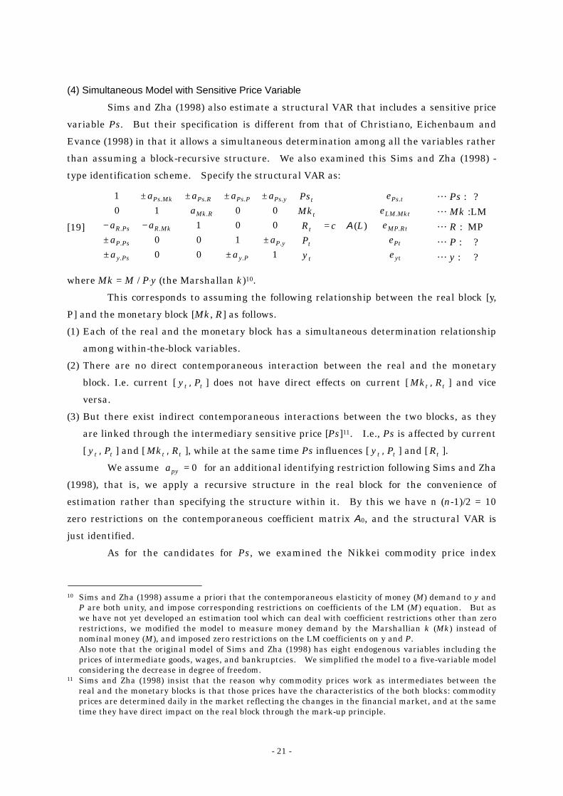
(4) Simultaneous Model with Sensitive Price Variable

Sims and Zha (1998) also estimate a structural VAR that includes a sensitive price

variable Ps. But their specification is different from that of Christiano, Eichenbaum and

Evance (1998) in that it allows a simultaneous determination among all the variables rather

than assuming a block-recursive structure. We also examined this Sims and Zha (1998) -

type identification scheme. Specify the structural VAR as:

… Ps : ? … Mk :LM … R : MP … P : ?

[19]

++=

±±±±

−−+

±±±±

t

)(

100

1000010010

1

y

Pt

MP.Rt

LM.Mkt

Ps.t

t

t

t

t

t

y.Py.Ps

P.yP.Ps

R.MkR.Ps

Mk.R

Ps.yPs.PPs.RPs.Mk

Lc

yP

RMk

Ps

aa

aaaa

a

aaaa

εε

εε

ε

A

… y : ?

where Mk = M / P.y (the Marshallan k)10.

This corresponds to assuming the following relationship between the real block [y,

P] and the monetary block [Mk, R] as follows.

(1) Each of the real and the monetary block has a simultaneous determination relationship

among within-the-block variables.

(2) There are no direct contemporaneous interaction between the real and the monetary

block. I.e. current [ tt Py , ] does not have direct effects on current [ tt RMk , ] and vice

versa.

(3) But there exist indirect contemporaneous interactions between the two blocks, as they

are linked through the intermediary sensitive price [Ps]11. I.e., Ps is affected by current

[ tt Py , ] and [ tt RMk , ], while at the same time Ps influences [ tt Py , ] and [ tR ].

We assume 0=pya for an additional identifying restriction following Sims and Zha

(1998), that is, we apply a recursive structure in the real block for the convenience of

estimation rather than specifying the structure within it. By this we have n (n-1)/2 = 10

zero restrictions on the contemporaneous coefficient matrix A0, and the structural VAR is

just identified.

As for the candidates for Ps, we examined the Nikkei commodity price index

10 Sims and Zha (1998) assume a priori that the contemporaneous elasticity of money (M) demand to y and

P are both unity, and impose corresponding restrictions on coefficients of the LM (M) equation. But as we have not yet developed an estimation tool which can deal with coefficient restrictions other than zero restrictions, we modified the model to measure money demand by the Marshallian k (Mk) instead of nominal money (M), and imposed zero restrictions on the LM coefficients on y and P. Also note that the original model of Sims and Zha (1998) has eight endogenous variables including the prices of intermediate goods, wages, and bankruptcies. We simplified the model to a five-variable model considering the decrease in degree of freedom.

11 Sims and Zha (1998) insist that the reason why commodity prices work as intermediates between the real and the monetary blocks is that those prices have the characteristics of the both blocks: commodity prices are determined daily in the market reflecting the changes in the financial market, and at the same time they have direct impact on the real block through the mark-up principle.

- 22 -

according to the original idea of Sims and Zha (1998)12, as well as the domestic WPI which

produced relatively good results in the previous section. We estimated ten specifications

each for the two candidates as usual, but the convergence was not achieved in eight cases

out of the total twenty.

Looking at the impulse responses for the estimated twelve cases (examples are in

Figure 4-1 and 4-2), the price puzzle is tenacious: P rises after a tight MP shock in all the

cases. There are also the cases in which y increases as well rather than decreases. The

positive responses of y and P to a tight LM shock are also observed in all the cases.

12 See the previous footnote.

- 23 -

Figure 4-1: Impulse Responses of the Simultaneous Structural VAR [Domestic WPI]



- 24 -

Figure 4-2: Impulse Responses of the Simultaneous Structural VAR [Commodity Price]



- 25 -

(5) Long-Run Neutrality Model

Blanchard and Quah (1989) use a long-run neutrality condition that the demand

does not affect the real variables in the long-run to identify the two variable AD-AS

structural VAR. The basic idea of the paper is as follows. Remember that a structural

VAR is expressed using the reduced form parameters B(L) and the contemporaneous

coefficients A0 as below (the constant term is suppressed for simplification).

[20] ttt L ε+= xAxA )(0 ttL ε+= xBA )(0

We can transform the structural VAR into a infinite vector moving average (VMA)

process of the structural shocks (the final form VMA).

[21] ttL ε=− xBIA )]([0 tt L ε1

01)]([ −−−=⇔ ABIx

Thus the matrix 10

1)]1([ −−− ABI (replacing the lag operator L with l) gives the

infinitely accumulated effects of the structural shocks ε. Long-run neutrality restrictions

corresponds to imposing zero restrictions on this matrix.

Now, recall the four-variable AD-AS model considered in Section 2-(1).

[22] IS)( ε+=−Ryy d [IS]

[23] LM)( ε+=+−+PRyMM d ,, [LM]

[24] MP)( ε−=++PyRR P , [MP]

[25] AS)( ε+=+Pyy S [Short-Run AS]

[25] is a short-run AS schedule, which is derived by incorporating labour demand

into a production function assuming nominal wage rigidity. However, wage will be flexible

in the long-run, and output will be determined solely by the supply side production

technology at the full employment GDP level (the Say’s low applies). Thus the long-run AS

schedule is:

[26] yyy .ASε+= ∗ [Long-Run AS]

A comparative statics of [22]-[24] and [26] gives the long-run effects of each shock.

This can be solved recursively as follows.

[26]’ ASεddy = [Long-Run AS]

[22]’ RyddydR )/( ISε+−= [IS]

Rydd )/( ISAS εε +−=

[24]’ Py RddRdyRdP ]/[ MPε++−= [MP]

PRy RdydddR ]/)/([ MPISASAS εεεε ++−+−=

PPRRy RdRyddyR /)/)1([ MPISAS εεε +++−=

- 26 -

[23]’ RRy yddMdMdM )/( ISASAS εεε +−−= [LM]

LMMPISAS /]/)1([ εεεε dRdMRyddyRM PPpRRyP ++++−+

PRRyPRRyP RydyRMMyMR /)]1()([ ASε+−+=

LMMPIS //)( εεε dRdMRydRMM PPPRPRP ++−+

The pattern of long-run effects of the each shock is therefore as expressed in the

following [27]. (Beware that the monetary policy [MP] equation is now assigned to the

equation, not to the call rate equation.)

………………… AS (y ) shock ………………… IS (R ) shock ………………… MP (P ) shock

[27]

++++−

+−+

=

M

P

R

y

dddd

dMdPdRdy

.

.

.

.

LM

MP

IS

AS

??000000

εεεε

………………… LM (M ) shock

We estimated a four variable AD-AS structural VAR using the long-run neutrality

identifying restrictions indicated by [27] (i.e. placing the zero restrictions indicated by the

matrix in [27] on the long-run effect matrix 10

1)]1([ −−− ABI ). If such restrictions lead to a

correct identification of the AD-AS structure supposed, then the estimated accumulated

impulse responses should show the pattern indicated in [27] in the long-run:

- Positive real supply (AS) shock ( yd .ASε > 0) will increase y, and decrease P and R

- Positive real demand (IS) shock ( Rd .ISε > 0) will not affect real output y in the

long-run, and the effect is absorbed by increases in P and. R

- Nominal shocks such as loose monetary policy (MP) shock ( Pd .MPε > 0) and tight

money demand (LM) shock ( Md .LMε > 0) will not affect the real sector variables y, P

Also, if the supposed AD-AS structure is identified correctly, the estimated

contemporaneous coefficient matrix A0 and the short term impulse responses should follow

those indicated by the short-run model [22]-[25] and its comparative statics.

……… y [AS] ……… R [IS] ……… P [MP]

[28]

+

+=

−−−

−

M

R

R

y

MPMRMy

PRPy

Ry

yP

MPRy

(L

MPRy

aaaaa

aa

.

.

.

.

Ac

LM

MP

IS

AS

)

101001001

εεεε

……… M [LM]

……………… AS (y ) shock ……………… IS (R ) shock ……………… MP (P ) shock

[29]

++++−−+−+++

=

M

R

R

y

dddd

dMdPdRdy

.

.

.

.

LM

MP

IS

AS

??000

εεεε

……………… LM (M ) shock

We estimated the structural VAR with such long-run neutrality identifying restrictions

for four specifications in which all the variables including interest rate R are differenced.

- 27 -

However, the results do not match with the expected ones.

Table 3 shows the estimated coefficient matrices and the accumulated long-run

impulse responses. The long-run response matrices show that the positive real supply (AS)

shock raises interest rate R and price P in the long-run against the expectation. We also

obtained unexpected signs in the coefficient matrices:

- AS curves are negatively sloped in the y-P plane, which is more plausible for AD curves.

- IS equations show positive relation of real demand and interest rate R.

- MP equations show that the authority lowers interest rate R when observing rise in P

in all the cases, and also on increase of y in two cases.

- LM curves are negatively sloped in R-M plane.

The estimated accumulated impulse responses in Figure 5 also exhibit unexpected

patterns of responses.

- Positive real supply (AS) shock rises R and P, at least from the second year.

- Positive real demand (IS) shock reduces output y.

- Loose monetary policy (MP) shock reduces y. Also it initially raises R.

The long-run neutrality restrictions examined here seem to be invalid in identifying

the supposed AD-AS structure of the Japanese economy.

Table 3: Coefficient Matrices and Accumulated Responses of the Long-Run Neutrality Model Log-Difference (1) [R: Difference] 2 Lags Log-Difference (1) [R: Difference] 4 Lags

Contemporaneous Coefficient Matrix A0 Contemporaneous Coefficient Matrix A0 0.1912 -0.2039 -0.1869 -0.1937

-0.1050 0.7899 0.1150 -0.1386

0.2251 -0.4367 0.7931 -0.1171

0.5389 0.2232 -0.0873 0.1827

0.1170 -0.2486 -0.0931 -0.1226

-0.1139 0.7188 0.1300 -0.0869

0.1381 -0.4422 0.8912 -0.0098

0.4380 0.2076 -0.0625 0.0624

Accumulated Response Matrix [I - B(1)]-1 A0-1 Accumulated Response Matrix [I - B(1)]-1 A0

3.47479 -0.00000 0.00000 0.00000 5.14359 0.00000 0.00000 0.00000 0.92302 1.45058 0.00000 0.00000 1.17077 1.39025 -0.00000 -0.00000 2.01446 0.50268 2.21543 0.00000 3.52587 1.15965 2.90230 0.00000 6.20508 0.85553 1.25750 2.94597 9.43098 2.26656 2.42692 2.80987


Contemporaneous Coefficient Matrix A0 Contemporaneous Coefficient Matrix A0 0.2284 -0.1275 0.1536 0.5359 0.0465 -0.1227 0.0853 0.2043 -0.2790 0.6578 -0.3397 0.2569 -0.2038 0.5415 -0.2574 0.4239 -0.0113 0.0914 0.9608 -0.0446 0.0324 0.1290 0.9362 -0.0459 -0.1707 -0.1696 -0.0011 0.1128 -0.0052 -0.0028 0.0007 -0.0002 Accumulated Response Matrix [I - B(1)]-1 A0 Accumulated Response Matrix [I - B(1)]-1 A0 10.84345 -0.00000 -0.00000 -0.00000 17.21526 0.00000 -0.00000 -0.00000 2.78044 3.82129 -0.00000 -0.00000 3.72458 3.46954 -0.00000 0.00000 8.45899 4.21020 8.14961 -0.00000 15.15581 2.63019 6.77458 -0.00000 21.37123 7.83934 9.03448 7.97082 36.09658 5.84950 1.92611 8.02057

Log-Difference (1): variables are log-differenced from the previous period, SA (except R) Log-Difference (4): variables are log-differenced from the same period of the previous year, not SA (except R) Unexpected signs of coefficients and accumulated responses are marked by shadings

- 28 -

Figure 5: Accumulated Impulse Responses of the Long-Run Neutrality Model

(1) Log-Difference (1)[R: Difference] 2 Lags


Documents

A Structural VAR analysis of the Monetary Policy in Japan · Rt Pt Mt yt t t t t t t t t MR yR MP RP My Ry Py M R P y L M P y a a a a a a a.... c A MP AS LM IS 1 0 0 0 1 1 0 1 0 e