Embed Size (px)
Citation preview

December 2017
OIES PAPER: WPM 75
A Structural Model of the World Oil Market: The Role of Investment Dynamics and Capacity Constraints
in Explaining the Evolution of the Real Price of Oil
Andreas Economou, Paolo Agnolucci,
Bassam Fattouh and Vincenzo De Lipis*

A Structural Model of the World Oil Market
i
The contents of this paper are the authors’ sole responsibility. They do not necessarily represent the
views of the Oxford Institute for Energy Studies or any of its members.
Copyright © 2017
Oxford Institute for Energy Studies
(Registered Charity, No. 286084)
With thanks to the Kuwait Foundation for the Advancement of Sciences for funding support.
This publication may be reproduced in part for educational or non-profit purposes without special
permission from the copyright holder, provided acknowledgment of the source is made. No use of this
publication may be made for resale or for any other commercial purpose whatsoever without prior
permission in writing from the Oxford Institute for Energy Studies.
ISBN 978-1-78467-097-9
DOI: https://doi.org/10.26889/9781784670979
* Andreas Economou, Doctoral Researcher, UCL Energy Institute and OIES Research Associate;
Paolo Agnolucci, Senior Lecturer, UCL Institute for Sustainable Resources; Bassam Fattouh, OIES;
and Vincenzo De Lipsis, Research Associate, UCL Institute for Sustainable Resources.
Corresponding author. Email: [email protected]

A Structural Model of the World Oil Market
ii
Contents
Contents ................................................................................................................................................. ii
Figures and Tables ............................................................................................................................... ii
Abstract .................................................................................................................................................. 1
1. Introduction ....................................................................................................................................... 2
2. A Review of the Supply Shock Measures of Crude Oil ................................................................. 5
2.1. Measure of flow supply shocks to global crude oil production ..................................................... 6
2.2. Measure of exogenous shocks to OPEC crude oil production .................................................... 9
2.3. Measure of endogenous shocks to global production capacity ................................................. 11
3. A Structural Model of the World Oil Market.................................................................................. 14
3.1. Data ............................................................................................................................................ 14
3.2. Structural VAR model ................................................................................................................. 14
3.3. Identification ............................................................................................................................... 15
4. Estimation Results .......................................................................................................................... 17
4.1. Responses to oil supply and oil demand shocks ....................................................................... 18
4.2. Historical decomposition of the real price of oil ......................................................................... 21
4.3. Empirical comparison with a structural VAR model of flow supply, flow demand and speculative
demand shocks ................................................................................................................................. 25
4.3.1. Responses of the real price of oil to oil supply and oil demand shocks .............................. 26
4.3.2. Contribution of the structural shocks to oil price movements since 2002 ........................... 27
4.3.3. Real-time forecasts of the Brent price as of June 2014....................................................... 28
5. Conclusion ....................................................................................................................................... 32
Acknowledgments .............................................................................................................................. 34
References ........................................................................................................................................... 35
Appendix A .......................................................................................................................................... 39
Appendix B .......................................................................................................................................... 40
Figures and Tables
Figure 1: Worldwide drilling activity and global capacity utilisation rates, 1975-2016 ............................ 4
Figure 2: World crude oil production in monthly percent changes, 1973.2-2016.8 ................................ 7
Figure 3: Exogenous disruptions and offsets in OPEC crude oil production in thousand barrels per day, 1990.1-2016.8 ......................................................................................................................................... 9
Figure 4: Measure of exogenous supply shocks to OPEC crude oil production in first-difference, 1990.2-2016.8 ....................................................................................................................................... 10
Figure 5: Endogenous cover/exposed levels of crude oil production in thousand barrels per day, 1990.1-2016.8 ....................................................................................................................................... 12
Figure 6: Measure of endogenous oil supply shocks to global production capacity in first-difference, 1990.2-2016.8 ....................................................................................................................................... 13
Figure 7: Structural impulse responses and corresponding pointwise 68% posterior error bands, 1990.2-2016.8 ....................................................................................................................................... 18
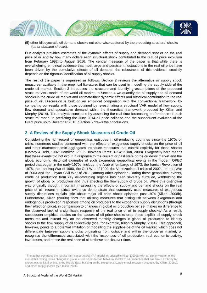
Figure 8: Historical decomposition of the real price of oil by structural shock in percent changes, 1992.2-2016.8 ....................................................................................................................................... 20
Figure 9: Contribution to the cumulative change in the real price of oil by structural shock, in 2016.8 USD per barrel ...................................................................................................................................... 22
Figure 10: Contribution to the cumulative change in the real price of oil by structural shock from January to August 2016, in 2016.8 USD per barrel .............................................................................. 23
Figure 11: Responses of global real economic activity and the real price of oil to a positive endogenous oil supply shock ................................................................................................................ 24

A Structural Model of the World Oil Market
iii
Figure 12: Structural impulse responses of the real price of oil by model specification, in percentages, 1990.2-2016.8 ....................................................................................................................................... 27
Figure 13: Contribution to the cumulative change in the real price of oil by structural shock, by model specification, in 2016.8 USD per barrel ................................................................................................ 28
Figure 14: One-step ahead forecasts of the Brent price for July 2014 to January 2015, in nominal USD per barrel, 2014.1-2015.1 ............................................................................................................. 29
Figure 15: One-step ahead forecast errors from September 2014 to January 2015 ............................ 30
Figure 16: Real-time forecasts of the Brent price as of December 2014, in nominal USD per barrel, 2013.12-2016.12 ................................................................................................................................... 31
Figure 17: Actual and predicted annual change of the key oil market indicators for 2015 and 2016, year-over-year ....................................................................................................................................... 32
Figure A1: Structural impulse responses and corresponding pointwise 68% posterior error bands conditional on the estimate of the 4-variable SVAR model, 1990.2-2016.8 ......................................... 39
Figure B1: Index of global real economic activity in percent deviations from trend, 2014.1-2015.1 .... 40
Table 1: Sign restrictions on impact responses in VAR model ............................................................. 16
Table 2: Minimum and maximum cumulative contribution to the real price of oil per range of price elasticity of oil demand in use, in percentages ..................................................................................... 25
Table 3: Sign restrictions on impact responses in the 4-variable SVAR model .................................... 26
Table 4: Recursive MSPE ratio of the baseline model forecast relative to the 4-variable SVAR model forecast .................................................................................................................................................. 31

A Structural Model of the World Oil Market
1
Abstract
Using novel measures that decompose oil supply shocks into its exogenous supply (driven by
exogenous geopolitical events in OPEC countries) and endogenous supply (driven by investment
dynamics within the oil sector) components, this paper offers a fresh perspective on the role of supply,
flow demand and speculative demand shocks in explaining the changes in the real price of oil over
the last three decades. We show that while exogenous supply shocks are non-negligible, endogenous
supply shocks have generated larger and more persistent price responses than previously thought.
Earlier studies have consistently shown that positive shifts in the flow demand for oil were responsible
for most of the oil price surge between 2002-2008. But this paper shows that endogenous production
capacity constraints, which restricted the ability of producers to ramp up production to meet the
unexpected increase in demand, added at least $50/barrel to the real price of oil. More recently,
endogenous oil supply shocks alone accounted roughly for twice as much as any other supply or
demand shock in explaining the 2014 oil price collapse. Specifically, of the $64 per barrel cumulative
decline in the real price of oil from June 2014 to January 2015, our model estimates that $29 have
been due to endogenous oil supply shocks, $13 have been due to exogenous oil supply shocks, and
$12 have been due to flow demand shocks. The paper concludes by demonstrating that forecasting
models that are able to distinguish between exogenous and endogenous supply shocks generate
more realistic out-of-sample estimates of the sequences of the structural shocks, thus resulting in
higher real-time predictive accuracy than forecasting models that use a collective measure of a flow
supply shock.
Keywords: Oil price; crude oil market; supply; demand; inventories; production capacity; OPEC; shale
oil; oil production; economic activity; oil shocks; forecast; structural model; VAR; identification.

A Structural Model of the World Oil Market
2
1. Introduction
Understanding the evolution of the oil price is important to consumers, firms and policymakers
because oil price fluctuations affect economic decisions across all segments of the global economy
(Barsky & Kilian, 2002, 2004; Hamilton, 2009a; Kilian, 2008a, 2014). Oil price fluctuations, however,
are difficult to anticipate due to unexpected shifts in supply and demand (Baumeister & Kilian, 2016a).
In practice, the oil price will only be as predictable as its determinants, implying that the better one
can identify and understand the determinants of past oil price fluctuations, the more realistic
interpretations and better forecasts one can make (Alquist, Kilian & Vigfusson, 2013; Baumeister &
Kilian, 2012, 2014). The unexpected component of a change in the price of oil is referred to as an oil
price shock, defined as the difference between the expected price of oil and its eventual realisation.
Just a few years ago, it was commonly believed that all major oil price shocks could be attributed to
oil supply disruptions triggered by exogenous geopolitical events in oil-producing countries, such as
wars and revolutions, and/or by some other disruptive supply-based factors, such as a shift in OPEC’s
oil policy (Hamilton, 1983, 1985, 2003).1 Today, this view has little empirical support. Not only do
direct measures of exogenous oil supply disruptions have little explanatory power (see, for example,
Kilian, 2006, 2008b), but also structural vector autoregressive (VAR) models of the world oil market
that focus on the supply-demand determinants of the oil price show that oil supply shocks overall
have had little impact on the real price of oil since 1973 (Baumeister & Peersman, 2013a, 2013b;
Kilian, 2009a; 2009b; Kilian & Murphy, 2014; Kilian & Hicks, 2013; Peersman & Van Robays, 2009).
In contrast, there is now widespread recognition that changes in crude oil demand best explain most
major oil price fluctuations since the 1970s. Demand shocks driven by shifts in the global business
cycle are now seen as the primary driver of oil prices, with shocks to physical speculative (or
inventory) demand arising from shifts in market participants about future supply-demand tightness
playing a much lesser part (see also Baumeister & Hamilton, 2015; Baumeister & Kilian, 2016b; Kilian
& Lee, 2014; Lippi & Nobili, 2012; Melolinna, 2012).
Although traditional supply-side explanations of the real price of oil have come under extreme scrutiny
during the past decade, there is still good reason to be sceptical of the assertion that the supply
determinant is not as important as originally thought. The classical notion of an oil supply shock as
discussed in the literature (also referred to as flow supply shock), corresponds to an exogenous
disturbance to the flow supply that shifts the upward-sloping oil supply curve along the downward-
sloping oil demand curve and hence, results in an opposite movement in global oil production and in
the real price of oil (see, for example, Baumeister & Peersman, 2013b; Kilian, 2009a; Kilian & Murphy,
2014). Recent experience, however, with regards to the oil price collapse in the second half of 2014,
when the monthly average real price of oil plunged by -44%,2 has shown that oil supply shocks can
generate abrupt changes in the real price of oil without large quantity movements, if at all, in the
observed global oil production. For example, Baumeister & Kilian (2016b) argue that to the extent that
oil supply shocks mattered for the 2014 oil price collapse, the question of interest is not whether oil
production moved or not, but whether it moved relative to what it was expected to be. The authors go
further and suggest (p. 135): “If oil production was expected to decline, for example, but did not
because of a positive oil supply shock, then this shock would trigger an additional [downward]
adjustment of the price of oil without a change in observed oil production”. In a falling market
characterised by relative oil abundance, such expectations could arise by beliefs that OPEC oil
1 Exogeneity here means that these events did not occur in response to the current or past state of the crude oil market and the
global economy. 2 The real price of oil in this paper refers to the Brent price deflated by the US consumer price index in August 2016 USD,
unless otherwise stated. The Brent price is the most widely traded global crude oil benchmark and refers to a light-sweet grade
of crude oil produced from several separate crude streams in the North Sea.

A Structural Model of the World Oil Market
3
producers will pursue an aggressive pricing strategy by curbing their output and/or non-OPEC oil
producers whose long-run marginal costs exceed the current price of oil will exit the market. An
opposite situation arises when the market is tight. If oil production is expected to increase, but does
not because of a negative oil supply shock, then this shock would trigger an additional upward
adjustment of the price of oil without a change in observed oil production (see, for example, Hamilton,
2009a). This phenomenon became self-evident during the 2003 and mid-2008 surge of the monthly
average real price of oil from $41/b to $147/b, driven by a series of stronger-than-expected flow
demand shocks in conjunction with a stagnating global oil production from 2004 onwards (Hamilton,
2009b, 2013a, 2013b; Kilian, 2009b, 2010a, 2010b; Lombardi & Van Robays, 2011; Nakov &
Pescatori, 2010). In both cases the heart of the problem is not the unexpected disruptions of global oil
production, but instead is the limited ability of oil producers to adjust oil supplies in response to
demand-driven shocks to the real price of oil, due to the presence of capacity constraints in crude oil
production (see Baumeister & Kilian, 2016a; Kilian, 2008b; Mabro, 1998, 2006; Smith, 2009). Indeed,
there is a consensus in the literature that the absence of surplus production capacity since the early-
1990s may have contributed to higher oil price fluctuations, albeit quantifying the extent of these
changes has proved hard to empirically pin down (see, for example, Baumeister & Peersman, 2013a).
Traditional oil market VAR models implicitly assume that existing production capacity in oil producing
countries is fixed over time, while the ability or willingness of oil producers to adjust production to
smooth out price changes is observationally equivalent to a shock to the flow supply of crude oil, as
measured by global crude oil production (see, for example, Kilian & Murphy, 2014). 3 Capacity
constraints however are not fixed over time and the outcome of a given exploration effort are not
related to prices; in contrast the investment decision is (Favero & Perasan, 1991; Mabro, 1992). As
noted by Fattouh and Mabro (2006) a number of uncertainties pertaining to geological, political,
economic and technological factors have an impact on the investment decisions of oil producers, that
affect oil supply and can lead to inefficiencies. On the one hand, considering the long lead times and
long gestation periods from the point at which a Final Investment Decision (FID) is made and the start
of first-production, underinvestment in upstream oil can generate large oil price spikes due to the
inability of oil producers to maintain and expand production. On the other hand, considering that once
costs have been sunk producers are unlikely to reverse an investment decision on a project, as well
as shutting-in operating capacity is costly, overinvestment in upstream oil can depress the price of oil
due to the unwillingness of oil producers to defer excess production. Even OPEC will find it difficult to
maintain its role as a market stabilizer in an oversupplied market because of the uncertainty
pertaining to the responsiveness of oil demand and non-OPEC supply to a higher price, as well as the
cost of losing market share in favour of restoring its revenue (Fattouh & Sen, 2015). Taken together,
whereas both risks of either under- or over-investment can result to capacity constraints in crude oil
production, their effect on the real price of oil would be markedly different. This point is displayed in
Figure 1 that shows the annual worldwide active rig counts (i.e. drilling activity) as one of the primary
indicators for investment activity in the oil sector and the global capacity utilisation rates for the period
1990-2016. As is evident from both graphs, the presence of capacity constraints due to
underinvestment refers to a situation where the current or future production capacity is unable to meet
the current or expected increases in global oil demand (as observed by the profound year-on-year
increases in drilling activity during 2003-2008), generating thus abrupt and persistent increases in the
real price of oil. In contrast, the presence of capacity constraints due to overinvestment refers to a
situation where the current and future operating capacity runs ahead of the current and expected
increases in oil demand, thus severely depressing the real price of oil and producing an environment
conducive to low investment rates affecting supply conditions in the next cycle (as observed by the
more-than-halve displacement of drilling rigs during 2014-2016). Such asymmetric responses are not
3 Production capacity is the sum of operating and spare (or surplus) capacity. Operating capacity is defined as the maximum
sustainable amount of capacity that is in operation at the beginning of a period. Spare capacity is defined as the component of
production capacity that is not in operation but can be brought online within one month; or not in operation but under active
repair that can be completed within three months.

A Structural Model of the World Oil Market
4
allowed for in the existing VAR literature in modelling the world oil market, which implies that this type
of oil supply shocks cannot be identified from traditional observables of flow supply. This observation
raises the question of how reliable is the comparative lack of explanatory power of the supply
determinants in favour of the demand-driven explanations of major fluctuations in the real oil price.
Figure 1: Worldwide drilling activity and global capacity utilisation rates, 1975-2016
Notes: The real price of oil refers to the West Texas Intermediate price deflated by the US consumer price index in 2016 USD. The red shaded bars indicate the periods 2003-2008 and 2014-2016. Data source: Federal Reserve Bank of St. Louis; Baker Hughes GE Database; US Energy Information Administration.
This paper quantifies the role of investment dynamics and capacity constraints in crude oil production
in determining the real price of oil, by redefining oil supply shocks in terms of exogenous geopolitical
disruptions in crude oil production (henceforth referred to as exogenous supply shocks) and the
presence of capacity constraints in crude oil production due to investment dynamics (henceforth
referred to as endogenous supply shocks). The identification of the newly proposed oil supply shocks
rests on the availability of two time series due to Economou (2016). One is a measure of exogenous
production shortfalls of crude oil due to geopolitical events in OPEC producing countries. The other is
a newly constructed time series intended to capture any positive (oversupply) and negative (stagnant
supply) deviations of production capacity from the equilibrium production path that arise due to risks
of either over- or under-investment, respectively, and due to the presence of capacity constraints in
crude oil production. Accordingly, the analysis in this paper builds on a fully specified structural vector
autoregressive (VAR) model of the world oil market, in the tradition of Kilian and Murphy (2014), that
decomposes the real price of oil as follows:
(1) shocks to oil supply that are caused by exogenous geopolitical events in OPEC countries (exogenous supply shocks);
(2) shocks to oil supply that arise within the crude oil market due to investment inefficiencies in upstream oil that result to capacity constraints (endogenous supply shocks);
(3) shocks to oil demand associated with the global business cycle (flow demand shocks);
(4) shocks to stock demand arising from the forward-looking behaviour of the market participants (speculative demand shocks); and
A Structural Model of the World Oil Market
5
(5) other idiosyncratic oil demand shocks not otherwise captured by the preceding structural shocks (other demand shocks).
Our analysis provides estimates of the dynamic effects of supply and demand shocks on the real
price of oil and by how many dollars each structural shock contributed to the real oil price evolution
from February 1992 to August 2016. The central message of the paper is that while there is
overwhelming empirical evidence that most large and persistent fluctuations in the real oil price have
been driven by the cumulative effects of oil demand, the robustness of this evidence crucially
depends on the rigorous identification of oil supply shocks.
The rest of the paper is organised as follows. Section 2 reviews the alternative oil supply shock
measures, available in the empirical literature, that can be used in modelling the supply side of the
crude oil market. Section 3 introduces the structure and identifying assumptions of the proposed
structural VAR model of the world oil market. In Section 4 we quantify the oil supply and oil demand
shocks in the crude oil market and estimate their dynamic effects and historical contribution to the real
price of oil. Discussion is built on an empirical comparison with the conventional framework, by
comparing our results with those obtained by re-estimating a structural VAR model of flow supply,
flow demand and speculative demand within the theoretical framework proposed by Kilian and
Murphy (2014). The analysis concludes by assessing the real-time forecasting performance of each
structural model in predicting the June 2014 oil price collapse and the subsequent evolution of the
Brent price up to December 2016. Section 5 draws the conclusions.
2. A Review of the Supply Shock Measures of Crude Oil
Considering the rich record of geopolitical episodes in oil-producing countries since the 1970s-oil
crisis, numerous studies concerned with the effects of exogenous supply shocks on the price of oil
and other macroeconomic aggregates introduce measures that control explicitly for these shocks
(Dotsey & Reid, 1992; Hamilton, 2003; Hoover & Perez, 1994; Kilian, 2008). Exogeneity here means
that these events did not occur in response to the current or past state of the crude oil market and the
global economy. Historical examples of such exogenous geopolitical events in the modern OPEC
period that began in the early-1970s, include: the Arab oil embargo of 1973, the Iranian Revolution of
1978, the Iran-Iraq War of 1980, the Gulf War of 1990, the Venezuelan oil crisis of 2002, the Iraq War
of 2003 and the Libyan Civil War of 2011, among other episodes. During these geopolitical events,
crude oil production from key oil-producing regions has been severely curtailed, withholding the
growth of global oil production and thus affecting the flow supply of crude oil. While this distinction
was originally thought important in assessing the effects of supply and demand shocks on the real
price of oil, recent empirical evidence demonstrate that commonly used measures of exogenous
supply disruptions explain little about major oil price shock episodes post-1974 (Kilian, 2008b).
Furthermore, Kilian (2009a) finds that utilising measures that distinguish between exogenous and
endogenous production responses among oil producers to the exogenous supply disruptions (through
their effect on price), in comparison to changes in global oil production per se, makes no difference to
the observed lack of a significant response of the real price of oil to supply shocks.4 As a result,
subsequent empirical studies on the causes of oil price shocks drop these explicit oil supply shock
measures and instead rely on the observed monthly changes in global oil production to identify
shocks to the flow supply of oil collectively (see, for example, Kilian & Murphy, 2014). This approach,
however, points to a potential limitation of modelling the supply-side of the oil market, which does not
differentiate between supply shocks originating from outside and within the crude oil market, or
recognise the differences associated with the responses of oil production, real economic activity,
inventories, and hence the real price of oil to these shocks over time.
4 The author compares the results from the structural VAR model introduced in Kilian (2009a) with an earlier version of the
model that distinguishes changes in global crude oil production between shocks to oil production that are driven explicitly by
exogenous political events in the Middle East, building on the exogenous supply shock measure proposed by Kilian (2008b),
and other supply shocks (see Kilian, 2006).

A Structural Model of the World Oil Market
6
In addressing these problems, recent empirical work by Economou (2016) introduces a new set of oil
supply shock measures that distinguish between changes in crude oil production that arise due to
exogenous geopolitical events in OPEC producing countries, such as wars and civil unrests, and
capacity constraints in production capacity that arise due to market-specific innovations associated
with the investment dynamics in upstream oil. The key insight on which the proposed measures are
built is that any attempt to identify the timing and magnitude of these distinct oil supply shocks
requires explicit assumptions about the counterfactual path of oil production in the absence of an
exogenous event in question on the one hand and conditional to the equilibrium production path on
the other hand. The methodology for constructing the exogenous oil supply shock measure
generalises the approach introduced by Kilian (2008b) and is designed to capture the timing, the
duration, the magnitude and the sign of all exogenous changes in OPEC crude oil production driven
by major geopolitical events. The newly proposed measure of endogenous supply shocks builds on
the explicit assumption that oil supply shocks can also be determined endogenously with respect to
the cumulative amount that could eventually be extracted and the projected time path of the demand
function (Adelman & Watkins, 2008; Smith, 2009, 2012). The reasoning underlying this assumption
follows the logic that just as the interaction of supply and demand determines the equilibrium price
path, these market forces determine also the equilibrium production path (Adelman, 1993).
Accordingly, the endogenous oil supply shock measure is designed to capture the timing, the
magnitude and the sign of any positive or negative deviations of production capacity from the
equilibrium production path that arise due to inefficiencies in the investment decisions of oil
producers. These measures allow us to evaluate the quantitative importance of the exogenous and
endogenous supply components in the real price of oil at each point in time since January 1990. This
is a period of academic and policy interest, as the supply-side of the oil market experienced a
structural shift away from the problem of availability towards the problem of deliverability5 and the
investment challenge that dictate oil price dynamics to date (Fattouh & Mabro, 2006).
2.1. Measure of flow supply shocks to global crude oil production
The classical notion in the literature of shocks to the flow supply of crude oil, associates these shocks
with disruptions in global oil production driven by exogenous geopolitical events in oil-producing
countries, as well as politically motivated decisions by OPEC members and other flow supply-related
shocks (Kilian & Murphy, 2014, p. 458). Figure 2 plots the monthly percent changes in global crude oil
production from February 1973 to August 2016, using data compiled by the US Energy Information
Administration (EIA). From the figure, it is shown that major historical movements in crude oil
production reflect largely key exogenous geopolitical events in OPEC countries (indicated by the
vertical lines in the plot), which are associated with wars and political unrests, politically motivated
supply decisions and internal OPEC power struggles observed during periods of high volatility such
as in the mid-1980s (see Gately, Adelman & Griffin, 1986). It can also be seen that, by historical
standards, there have been no substantial fluctuations in global oil production after 1990, with the
largest changes corresponding to the Gulf War of 1990, the Venezuelan Oil Crisis of 2002 and the
Iraq War of 2003.6 Indicatively, from January 1990 to August 2016, shocks to the flow supply of oil
accounted for 0.8% of the variability in global oil production changes, compared to 4.8% in the
previous period of the sample (February 1973 to December 1989). Finally, a visual examination of the
series seems to belie any obvious relationship to endogenous shocks in crude oil production after
2003. Yet a large body of the recent literature postulates that major oil price developments after 2003
were partly driven by capacity constraints in crude oil production associated with the long run
5 Naimi (2005) defines deliverability as a measure of effective capacity that the oil industry needs to develop, produce, refine
and deliver to end-consumers, as to meet the actual and expected oil demand. 6 The volatility starting from mid-1990s till the early-2000s is largely driven by the fluctuations in Iraqi oil production associated
with the gradual erosion of the U.N. Oil-for-Food-Programme and the Iraqi oil exports bans that served as a negotiating tactic
against the uneven enforcement of the U.N. sanctions (Katzman, 2003).

A Structural Model of the World Oil Market
7
challenges of depletion, the erosion of spare capacity, the economic viability of new sources of supply
such as US shale oil and Canadian oil sands, as well as shifts in OPEC oil output policy (Alquist &
Guenétte, 2014; Arezki, 2016; Fattouh & Sen, 2015; Hamilton, 2013a, 2014; Sandrea, 2014).
A case in point is the 2003-2008 episode, during which the strong demand growth from the non-
OECD economies had caught up with the decade-long structural underinvestment in the upstream
sector of the 1990s, the maturity of legacy oil fields and the long lead times associated with the
development of new production capacity. Between 2004 and 2007, oil consumption in emerging
economies increased on average by a 4.3% annual growth rate, whereas global oil production
between 2005 and 2007 unexpectedly halted.7 Although there have been other episodes when global
oil production stagnated over a two-year period, these were inevitably either responses to falling
demand during recessions or to exogenous supply disruptions (Hamilton, 2013b). During this episode,
however, the strength of global demand growth caught oil producers by surprise. By 2007, crude oil
production outside OPEC was 0.73 mb/d lower from its levels in 2004, as important contributors to the
growth of non-OPEC oil supply (e.g. the US, the North Sea and Mexico) failed to maintain and expand
production. Fattouh & Mabro (2006) attribute this stagnation of crude oil production to a number of
economic, political and geological factors, as well as other relating to corporate behaviour, that
predominated in the oil industry since the 1980s. These factors combined produced a long-lasting
environment conducive to low investment rates in the upstream sector at the expense of maintaining
and developing new crude capacity. Most importantly, the main impact of the generalised structural
underinvestment in the upstream sector over the previous two decades was felt on the erosion of
spare capacity that between 2002 and 2005 collapsed by 4.15 mb/d, down to 1.02 mb/d (Fattouh,
2006). Hamilton (2009b, p.10) characterises the 2003-2008 oil price surge as a new era for oil price
dynamics, according to which without the willingness or the ability of Saudi Arabia to adjust production
to smooth out price changes, any disturbance to supply or demand had a significantly bigger effect on
price after 2005.
Figure 2: World crude oil production in monthly percent changes, 1973.2-2016.8
7 Calculations in this section are based on publicly available data from the US Energy Information Administration, unless stated
otherwise. Available at: https://www.eia.gov/petroleum/data.php

A Structural Model of the World Oil Market
8
Another case of interest, is the unprecedented growth of US shale oil production and its importance to
recent price dynamics which shifted market perceptions from oil scarcity to oil abundance. Between
2009-2015, US oil production grew on average at a sustained annual rate of 9.6%, while US shale oil
production alone grew on average by a remarkable annual rate of 22.3%. Alquist and Guenétte
(2014) attribute this unprecedented growth in US shale oil production to the persistent high oil prices
in the past decade, the transfer of technological expertise and knowledge from the exploitation of
shale gas that had been developed in the US since the 19th century, as well as the legal incentives,
access to finance and advanced infrastructure available to US oil producers. Nevertheless, despite
US oil production accounting on average for 9% of total world output (between 2009-2015), the
immense growth of US production had no obvious impact to the growth of global oil production, at
least not until 2014. Many observers have suggested that this paradox can be explained by the fact
that from December 2010 to March 2014, the 3.2 mb/d of new production originating from the US
were exactly matched by exogenous disruptions in oil production in the Middle East and North Africa
(Stevens, 2015, p. 6). Only in the second half of 2014, when the earlier geopolitical production
shortfalls unexpectedly receded and OPEC decided not to cut output to counter the excess supply
that had been muted for years, did the supply-demand imbalance materialise, generating a very
significant price response to the downside (Baffes et al. 2015). By 2015, the annual average real price
of oil halved from $100/b down to $53/b, as global oil production continued to grow at an annual
average rate of 2.8% driven by an increase in OPEC and US crude oil production by 4% and 7.4%
respectively, while global oil consumption grew by a comparably weaker annual average rate of 1.6%.
Evidently, there is a good reason to suspect that modelling shocks to the flow supply of oil collectively,
based on changes in global oil production per se, may render recent structural VAR models of the
world oil market informationally mispecified. One important implication is that critical information about
the underlying supply conditions of the crude oil market are not contained in the shock measure of
flow supply available to the econometrician (e.g. oil production might be subject to capacity
constraints). An additional implication is that exogenous shocks in crude oil production would be
expected to have a markedly different effect on the real price of oil, as on the rest variables of the
model, compared to shocks to crude oil production within the confines of the world oil market. To the
extent that this assumption is valid, estimates of the dynamic effects of flow supply shocks on the real
oil price are potentially misleading, especially at increasingly distant horizons. The reason is that, on
the one hand, geopolitical shortfalls in crude oil production tend to be resolved in the short-run by
spare capacity releases when excess production is available, which explains why recent empirical
studies find that exogenous supply shocks have little systematic impact on the real price of oil (see,
for example, Kilian, 2008b). On the other hand, unless oil demand deteriorates, capacity constraints
due to underinvestment can only be resolved in the long-run by adding new capacity in the oil market,
which is a process associated with long gestation periods and lead times of optimal investment
decisions and planning (Fattouh & Mabro, 2006). Similarly, unless oil demand recovers or OPEC
collectively decides to balance the market, the only way to resolve capacity constraints due to
overinvestment hitting the market, is for oil producers whose long-run marginal cost exceeds the
current price of oil to exit the market, which can take months or years (Baumeister & Kilian, 2016b).8
This line of reasoning suggests that while exogenous oil supply shocks are non-negligible, capacity
constraints in crude oil production may have generated larger and more persistent price responses in
recent years than previously thought.
8 In his regard, Adelman (1962) notes that, under competition, when demand falls short of operating capacity the price must fall
so low until it is clearly below the current extractive operation costs of many wells producing a sizeable fraction of output, for the
market oversupply to be resolved.

A Structural Model of the World Oil Market
9
2.2. Measure of exogenous shocks to OPEC crude oil production
Many studies have proposed measures of exogenous oil production shortfalls (see Dotsey & Reid,
1992; Hamilton, 2003; Kilian, 2008b). More recently, Economou (2016) proposes a monthly measure
of exogenous shocks to OPEC crude oil production that takes full account of the timing and the actual
duration of the shock, as well as of variations over time in its magnitude and sign. Building on the
work of Kilian (2008b), the author generates the counterfactual production level for an OPEC country
associated with an exogenous geopolitical episode, by extrapolating its pre-shock production level
based on the average growth rate of production in other OPEC countries that are subject to similar
governance, operational and investment performance but not in any way associated with that episode
or any other exogenous episode of their own. Incorporated into the counterfactual underlying the
construction of the series, is a monthly dummy variable that identifies the actual duration of an
exogenous shock to crude oil production on a case-by-case basis. This approach allows for the
counterfactual production level to normalise relative to actual production, given that the initial
exogenous event has expired and is not followed by another episode. Explicit in the methodology is
the role of Saudi Arabia which is the only producer that has an official policy of maintaining spare
capacity and has historically acted as a swing producer filling the gaps at times of oil disruptions
(Fattouh & Mahadeva, 2013). In this case, the counterfactual production series identifies the timing,
the magnitude and the sign of a Saudi oil production response to an exogenous production shortfall
elsewhere in OPEC, over an extended period of adjustment and not strictly temporary. The measure
of exogenous oil supply shocks reflects changes in OPEC crude oil production driven explicitly by
geopolitical events and not by collective output adjustment decisions in response to the state of the
crude oil market or by other oil market-specific factors (e.g. geological depletion or investment
decisions).9
Figure 3: Exogenous disruptions and offsets in OPEC crude oil production in thousand barrels
per day, 1990.1-2016.8
9 For a detailed discussion on the methodology and construction of the counterfactuals on a country-basis the reader is referred
to Economou (2016).

A Structural Model of the World Oil Market
10
Figure 3 shows the OPEC-wide exogenous shortfalls and offsets in crude oil production driven by
major geopolitical events for the period January 1990 to August 2016. These are computed on a
country-basis by subtracting from the actual production levels the constructed counterfactual levels at
monthly frequency. The negative production levels at each point in time may be viewed as the true
shortfalls in crude oil production from a given country as a response to a major exogenous event,
indicated by the vertical lines in the plot; namely from Iran, Iraq, Kuwait, Venezuela, Nigeria and
Libya. The positive production levels at each point in time may be viewed as the true oil production
responses from Saudi Arabia that are triggered in response to an exogenous event elsewhere in
OPEC. The actual duration of each exogenous shock to crude oil production is part of the propagation
mechanism to be estimated by the dummy series underlying the construction of the counterfactuals.
By summing all OPEC country-specific shortfalls in oil production and the Saudi production increases
as a response, it is possible to construct an aggregate time series of changes in OPEC crude oil
production caused explicitly by exogenous geopolitical events. The change over time in the series
provides a natural measure of the exogenous oil supply shocks at monthly frequency, shown in Figure
4. The series is expressed as a percent share of global production capacity.
Figure 4: Measure of exogenous supply shocks to OPEC crude oil production in first-
difference, 1990.2-2016.8
Figure 4 shows that exogenous oil supply shocks range from -7.5% to +4.5% of global production
capacity. These are associated with large negative and positive swings in OPEC crude oil production
that by construction reflect a production shortfall driven by an exogenous event and the degree of a
reversal of that shortfall either by releases of spare capacity from Saudi Arabia, or by the gradual
recovery of the initial shortfall following the expiration of the exogenous episode, or both. Exogenous
oil supply shocks from February 1990 to December 2003 account for 1.6% of the variability in global
production capacity changes, following the outbreak of major geopolitical events such as the Gulf War
of 1990, the Iraqi Oil Embargos during 1997-2002, the Venezuelan Oil Crisis of 2002 and the Iraq War
of 2003. From January 2004-onwards, however, the movements in the exogenous oil supply shock
measure are comparably weaker and less persistent, accounting for only 0.6% of the variability in
global production capacity. Overall, these exogenous movements exhibit a similar pattern with shocks
to the flow supply of oil as shown in Figure 2, the latter accounting for 1.2% and 0.4% of the variability
in world output at the same intervals, while a preliminary statistical comparison shows that the two

A Structural Model of the World Oil Market
11
measures are relatively close with a correlation of about 60%. This statistically significant relationship
further strengthens our concerns that measures of flow supply shocks may have become less
informative in recent years. One possible explanation is that they largely reflect changes in global oil
production that are brought about by exogenous events, thus neglecting important information about
innovations to oil production that arise within the crude oil market. Another explanation ex ante is that
to the extent that measures of flow supply shocks fail in practice to model the supply-side of the oil
market collectively, recent VAR models of the world oil market may ignore the endogenous channel of
transmission of supply shocks to the real price of oil, in favour of other demand-related channels.
Therefore, of equal importance to a measure that controls explicitly for all exogenous shocks to crude
oil production, is an explicit measure of shocks to global production capacity that operate within the
crude oil market.
2.3. Measure of endogenous shocks to global production capacity
Exogenous shocks to global crude oil production constitute only one type of oil supply shock. There
also may be shocks to global production capacity due to a number of uncertainties impacting the
investment decisions of oil producers and hence affecting the oil supply. This type of oil supply shocks
(referred to as endogenous oil supply shocks) arises within the crude oil market and implicitly reflects
the rate of investment in new production capacity, conditional to the expectations of oil producers
regarding future market conditions and the likelihood of price (Adelman, 1993; Mabro, 2006).
Accordingly, recent empirical work by Economou (2016) introduces a novel methodology for
constructing a monthly measure of endogenous oil supply shocks that takes full account of the timing,
the magnitude and the sign of any supply-related deviations from the equilibrium production path
driven by oil market-specific factors. The newly proposed measure implicitly equates new additions in
production capacity with oil production based on the critical assumption that just as the growth rate of
production capacity must be equal to that of oil production, the growth rate of oil production must be
approximately equal to that of petroleum consumption. Having adjusted the actual oil production
levels insofar as all exogenous shocks are accounted for (due to the measure of exogenous supply
shocks),10 the author generates the counterfactual production path for selected oil producers that are
net importers and net exporters by country, by extrapolating their adjusted production levels based on
the growth rate of their domestic consumption. The latter is weighted according to the percent
contribution of domestic production and imports drawn by origin to the total consumption of the net
importers, and the percent contribution of total production from the net exporters to domestic
consumption and exports by destination. The assignment of weights ensures that the counterfactual
production levels do not overstate the true endogenous shortages or surpluses in global oil
production, given that operating capacity is predetermined. The strategy is to estimate that amount of
oil production that the net importers need to cover by imports drawn to meet total domestic
consumption on the one hand, and that amount that is available for exports given that the net
exporters cover their domestic consumption on the other hand. The intuition is that through petroleum
inter-regional movements they should offset one another, thus determining the equilibrium production
path, from which it is possible to observe the timing, the magnitude and the sign of any oil market-
specific supply deviations over time (see Economou, 2016).
Figure 5 shows the vertical differences between actual and counterfactual production levels by
country for selected oil producers that are net importers, namely for the US and China, and those that
are net exporters, namely for aggregate OPEC, Russia, Canada, Mexico and the North Sea (i.e. the
UK and Norway combined); along key oil market-specific events in the period January 1990 to August
2016. Incorporated into the weights underlying the construction of the counterfactuals for the net
10 Further to oil supply shocks that arise explicitly by exogenous events in OPEC countries, the author also controls for
exogenous production shortfalls that occur outside OPEC, namely for Canada, Mexico, the North Sea, the US and Rest of
World. These are primarily associated with natural disasters, such as the Katrina/Rita/Ivan and Gustav/Ike Hurricanes in the
USGC of 2005 and 2008, as well as other geopolitical outages that occurred in the Middle East and North Africa following the
2011 Arab Uprisings.

A Structural Model of the World Oil Market
12
exporters, is also demand for imports from Japan, India, IEA Europe and Rest of World.11 Excluding
the last aggregate, the selected sample combined represents on average a total of 81% of world oil
output and 79% of world petroleum consumption, in the twenty-six-year horizon of the sample. The
negative production levels at each point in time may be viewed as that amount of oil supply that the
net importers need to cover by imports drawn and not from domestic production. The positive
production levels at each point in time may be viewed as that surplus amount of oil supply that is
available to be exported by the net exporters, given that they cover in principle their own domestic
needs. The change over time in the series is driven explicitly by endogenous factors conditional to the
current and past state of the crude oil market. For example, increasing production could be driven
either by a significant oil discovery or by a past period of high investment rates in the upstream sector,
or both. On the other hand, declining production could be driven by the natural declining rates of oil
reserves or by a past period of structural underinvestment in the upstream sector, or both. In addition,
these changes reflect collective OPEC (and non-OPEC) output adjustment decisions based on
expectations about future market conditions and price. By summing all country-specific endogenous
shortages and surpluses in oil production and further subtracting any amount of spare capacity over
the buffer of 2.0 mb/d,12 it is possible to construct an aggregate time series of imbalances in global
production capacity caused explicitly by oil market-specific factors. The change over time in the series
provides a natural measure of the endogenous oil supply shocks at monthly frequency as shown in
Figure 6, expressed as a percent share of global production capacity.13
Figure 5: Endogenous cover/exposed levels of crude oil production in thousand barrels per
day, 1990.1-2016.8
11 IEA Europe includes Austria, Belgium, Czech Republic, Denmark, Estonia, Finland, France, Germany, Greece, Hungary,
Ireland, Italy, Luxembourg, the Netherlands, Poland, Portugal, Slovak Republic, Spain, Sweden, Switzerland and Turkey;
excluding Norway and the United Kingdom. 12 As an informal rule of thumb, oil market analysts suggest that OPEC needs to hold at least 5% of global oil demand in spare
capacity to enable it to stabilise the market, which equals on average around 4.0 mb/d for the period 1990-2016 (McNally,
2012). However, Saudi Arabia’s declared policy is to maintain a volume of spare capacity of 2-3 mb/d (Fattouh & Mabro, 2006,
p. 125). 13 For more details on the rationale and construction of this measure the reader is referred to Economou (2016).

A Structural Model of the World Oil Market
13
Endogenous oil supply shocks between February 1990 to August 2016 range from around +2.5% to -
2.5% of global production capacity and account for 3.1% of the variability in the changes of the world
series, compared to only 1.2% of the variability due to exogenous oil supply shocks (as shown in
Figure 4). The movements in the baseline endogenous oil supply shocks measure can be reconciled
with key market-specific oil dates, indicated by the blue vertical lines in the plot. For example, the
initially negative and then positive swings exhibited in the shock measure in 1998, 1999, 2008 and
2009 are consistent with the collective OPEC-non-OPEC output adjustment decisions related to the
market uncertainty in the aftermath of the Asian Financial Crisis of 1997 and the Global Financial
Crisis of 2008. In addition, the negative spikes between 2002-2004 reflect the erosion of spare
capacity amid the unexpected surge in non-OECD oil demand, owing to the generalised
underinvestment in the oil sector in the 1990s. Finally, there are two periods of gradual fluctuations in
the endogenous oil supply shock series that denote persistence: the 2005-2008 and the 2012-2015.
The former reflects the global production stagnation associated with persistent declines in the series
followed by temporary increases, while the latter reflects the US capacity expansions in
unconventional oil production associated with persistent increases in the series followed by temporary
declines. Overall, endogenous oil supply shocks from February 1990 to December 2003 account for
1.9% of the variability in global production capacity changes, compared to 4.2% from January 2004-
onwards. A visual examination of the constructed series confirms that the measure is reasonably
isolated from any exogenous events, as indicated by the absence of any significant shortfalls during
key exogenous oil dates (e.g. Gulf War in August 1990). Furthermore, the correlation of the
exogenous and endogenous shock series is weak at about 20%. Similar results also hold when the
endogenous measure is compared with that of flow supply shocks (the correlation is weak at 21%).
This evidence supports the robustness of the endogenous oil supply shock measure, while further
strengthening the claim that traditional shock measures may neglect critical information about the
underlying supply conditions of the crude oil market.
Figure 6: Measure of endogenous oil supply shocks to global production capacity in first-
difference, 1990.2-2016.8

A Structural Model of the World Oil Market
14
3. A Structural Model of the World Oil Market
The analysis in this paper builds on a dynamic simultaneous equation model in the form of a structural
VAR that generalises the structural oil market model introduced by Kilian and Murphy (2014). The
sample period extends from February 1990 to August 2016. The model is specified based on a
monthly dataset that includes: (1) a measure of exogenous oil supply shocks; (2) a measure of
endogenous oil supply shocks; (3) a measure of global real economic activity; (4) the real price of oil;
and (5) a proxy of global crude oil inventories. Furthermore, we consider 24 autoregressive lags in
line with the literature (Hamilton & Herrera, 2004; Kilian, 2009a), an intercept and seasonal dummies
to remove the seasonal variations. The structural VAR model is set-identified based on a combination
of sign restrictions, as well as bounds on the impact price elasticities of oil supply and oil demand. 14
These identification restrictions constitute an essential component for the economic interpretation and
causal meaning of the model estimates and they are motivated by economic theory, institutional
knowledge and other extraneous information. The implementation of the identification procedure is
described in Kilian and Murphy (2014, p. 463), while for a general exposition about the usefulness of
set-identified VAR models the reader is referred to Kilian and Murphy (2012).
3.1. Data
Consider a VAR model based on monthly data for yt = (prodt, capt, reat, ∆rpot, ∆stockst)´. Accordingly,
prodt is the measure of changes in OPEC crude oil production driven by exogenous geopolitical
events in OPEC countries and capt is the measure of imbalances in global production capacity that
arise within the crude oil market, as discussed in Section 2. Both these measures are expressed as a
percent share of global production capacity and are stationary by construction. The reat denotes an
updated measure of global real economic activity proposed by Kilian (2009a). This is a business cycle
index of global real economic activity that is designed to capture shifts in the global demand for all
industrial commodities. Moreover, it is widely characterised by the literature as one of the most
suitable indices deemed appropriate for quantifying the effect of global economy on oil demand (see,
for example, Baumeister & Peersman, 2013a; Kilian & Hicks, 2013). The index is expressed as
percent deviation from a linear trend and is stationary by construction. The ∆rpot refers to the real
price of oil defined as the spot Brent price deflated by the US consumer price index and is expressed
in log-differences. Finally, ∆stockst is the level-changes in closing OECD crude oil and other liquids
inventories in million barrels, as reported by the EIA. Considering that there are no readily available
data in the public domain for global oil inventories, we follow the literature in approximating the global
stocks based on OECD oil inventories (see Hamilton, 2009b). Moreover, recent empirical studies that
device alternative proxies for above-ground global crude oil inventories show that the use of these
proxies in determining the real price of oil yields very similar results in general (see Kilian & Lee,
2014). This issue was addressed as part of our sensitivity analysis from which we concluded that the
use of alternative inventory data does not change the main results of this paper.
3.2. Structural VAR model
Let yt be a vector of the five observables, then the proposed structural VAR of the world oil market
may be written as:
𝐵0𝑦𝑡 = ∑ 𝐵𝑖𝑦𝑡−𝑖 + 𝜀𝑡
24
𝑖=1
, (1)
where 𝐵𝑖, 𝑖 = 0, …, 24, denotes the coefficient matrices and 𝜀𝑡 is the vector of orthogonal structural
innovations. The vector 𝜀𝑡 consists of five structural shocks. The first shock incorporates shocks to
14 Identification by sign restrictions in structural VAR models was pioneered by Faust (1998), Canova and De Nicolo (2002) and
Uhlig (2005). The refinements of these sign restrictions to accommodate additional inequality restrictions for reducing the set of
admissible structural models, as proposed in this paper, were introduced by Kilian and Murphy (2012).

A Structural Model of the World Oil Market
15
crude oil production triggered by geopolitical events in OPEC countries that are exogenous with
respect to the crude oil market (exogenous oil supply shock).
The second shock captures unexpected imbalances in production capacity, relative to the equilibrium
production path, that reflect the failure of oil producers either to expand production due to
underinvestment or to adjust excess production due to overinvestment, conditional on their
expectations about future market conditions and the likelihood of price (endogenous oil supply shock).
The third shock corresponds to unexpected fluctuations in the global business cycle that drive
demand for crude oil and other industrial commodities (flow demand shock).
The fourth shock captures changes in stock demand arising from forward-looking behaviour not
otherwise captured by the model (speculative demand shock).
Finally, the fifth shock corresponds to other idiosyncratic oil demand shocks that cannot be classified
as one of the preceding structural shocks (other demand shock). The latter is essentially a residual
shock that escapes economic interpretation, but it implicitly represents other exogenous shifts in the
demand for oil that can be driven by a myriad of reasons (e.g. weather-related shocks).
The preceding structural shocks are identified based on a set of key identifying assumptions that
involve primarily restrictions on the signs of the impact responses of the five observables to each
structural shock. These sign restrictions derive directly from the economic model, outlined as follows.
First, conditional on all past data, an unanticipated exogenous shortfall in crude oil production raises
the real price of oil and production capacity (through drilling activity), and lowers the real economic
activity on impact. The impact effect on oil inventories is ambiguous ex ante because inventories
could either be drawn down to mitigate the magnitude of the price increase (Hamilton, 2009b), or be
built up driven by speculative demand in anticipation of the price increase (Alquist & Kilian, 2010).
Therefore, we do not impose any restrictions on the sign of the impact response of oil inventories.
Second, an unanticipated endogenous contraction of production capacity causes the real price of oil
to increase and the real economic activity to decrease on impact. We do not restrict the sign of the
impact response of crude oil production and inventories because the former implicitly responds only to
exogenous events and the latter is ambiguous ex ante.
Third, an unanticipated increase in oil demand for current consumption (i.e. flow demand for oil)
raises the production capacity, the real economic activity and the real price of oil on impact. As in the
case of a negative endogenous oil supply shock, we do not impose any sign restrictions on crude oil
production and oil inventories.
Fourth, a positive speculative demand shock in equilibrium causes an accumulation in oil inventories,
which requires oil production to increase and oil consumption to decrease (reflected by an increase in
production capacity and a decline in real economic activity), as the real price of oil increases.15 By the
same logic as before, we do not restrict the sign of the impulse response of crude oil production to a
speculative demand shock.
Finally, these sign restrictions identify the fifth structural shock referring to other demand shocks not
otherwise accounted for.
3.3. Identification
The usefulness of identifying assumptions is that they allow the model to distinguish between the
unique patterns of the different oil supply and oil demand shocks, as well as they provide an
economically meaningful interpretation of the model estimates when assessing the causal effect of
these shocks to the model variables. Identification in set-identified models, however, can be
problematic in that the lack of sufficient information about the values of the structural model
15 For more details on the motivation, rationale and economic interpretation of speculative demand shocks the reader is referred
to Alquist & Kilian (2010) and Kilian and Murphy (2014).

A Structural Model of the World Oil Market
16
parameters can lead to a wide range of admissible models (i.e. satisfying the identification
restrictions), further complicating statistical inference (Inoue & Kilian, 2013). To overcome this
problem, Kilian and Murphy (2012) suggest that when such information exists it is important to impose
all credible identifying restrictions for the identification of the model estimates to be economically
meaningful. In particular, the authors demonstrate that sign restrictions may be strengthened with the
help of additional economically motivated inequality restrictions. In the context of a structural model of
the world oil market, one such set of restrictions relates to empirically plausible bounds on the
magnitude of the oil supply and oil demand elasticities on impact. Moreover, Kilian and Lütkepohl
(2017) argue that it is possible to further reduce the set of admissible model solutions by imposing
additional sign restrictions on the structural impulse responses beyond the impact period. However,
because it is difficult to imply these dynamic sign restrictions directly from economic theory, these are
often motivated based on some other extraneous information about the dynamic responses of the
model variables (see, for example, Inoue & Kilian, 2013). Accordingly, our structural VAR model is
identified based on a combination of static sign restrictions on the impact responses of the five
observables to each structural shock, dynamic sign restrictions on the responses to an unexpected
exogenous oil supply shock and bounds on the impact price elasticities of oil supply and oil demand.
Table 1: Sign restrictions on impact responses in VAR model
Exogenous supply shock
Endogenous supply shock
Flow demand shock
Speculative demand shock
Oil production – Production capacity
+ – + +
Real activity – – + – Real price of oil + + + + Inventories +
Table 1 summarises the sign restrictions on the impact responses of crude oil production, production
capacity, real economic activity, the real price of oil and oil inventories to each structural shock, as
described in Section 3.2. All structural shocks have been normalised as to imply an increase in the
real price of oil, while missing entries denote that no sign restrictions are imposed. In addition to these
static sign restrictions, we also impose the restriction that the response of the real price of oil to a
negative exogenous oil supply shock must be positive for at least one year beyond the impact period.
This implies a joint set of sign restrictions such that the responses of oil production and real economic
activity to an unanticipated exogenous oil supply shock are negative for the first twelve months, while
the responses of the real price of oil and production capacity are positive. The inclusion of these
dynamic sign restrictions follows the rationale in Kilian and Murphy (2014, p. 462), suggesting that
these are necessary to rule out admissible models in which unanticipated exogenous shortfalls in
crude oil production cause a decline in the real price of oil below its starting level. In contrast, we do
not impose any sign restrictions on the impulse responses to endogenous oil supply shocks, flow
demand shocks and speculative demand shocks beyond the impact period, because these shocks
are associated with an expectational component which is not possible to determine ex ante at
increasing horizons. For example, it is not possible to know how OPEC producers might resolve the
uncertainty pertaining to the future state of the crude oil market, nor how traders will respond to the
expectational shifts related to this uncertainty. These questions are instead treated as part of the
propagation mechanism to be estimated by the structural model, conditional to additional inequality
restrictions about the impact price elasticities of oil supply and oil demand.
The impact price elasticity of oil supply can be expressed as a function of the joint-ratio of the impact
responses of oil production and production capacity to an unexpected exogenous demand shock (i.e.
either in flow demand or in speculative demand), relative to the impact response of the real price of oil
triggered by the same shock. In practice, oil producers will be slow, if at all, to respond to a flow
demand shock on impact, given the costs of adjusting production and the uncertainty about the state
of the crude oil market (Kilian, 2009a). In support to this view are empirical estimates of the short-run

A Structural Model of the World Oil Market
17
price elasticity of oil supply that suggest a range between effectively zero and 0.27.16 Considering that
there is little evidence to suggest that differences within this range have an important effect on
inference about the relative contribution of oil supply and oil demand shocks on the real price of oil
(see, for example, Baumeister & Hamilton, 2015), we impose the restriction that the impact price
elasticity of oil supply falls within a lower bound of 0.00 and an upper bound of 0.02. This bound is
consistent with conventional views in the literature that suggest a steep but not quite vertical short-run
oil supply curve (Kilian & Murphy, 2014). We also examined the sensitivity of our main results to
higher upper bounds, indicatively of 0.05 and 0.1, and found that there are no significant changes to
the shape of the posterior distribution of the impulse responses, despite an increase in the set of the
admissible models, in line with the wider consensus in the literature.
Finally, the model imposes the restriction that the long-run price elasticity of oil demand must at least
weakly exceed on average the short-run price elasticity over the sample. Rather than associating this
oil demand elasticity with its textbook definition (i.e. the ratio of the impact response of oil production
and of the real price of oil to an unexpected oil supply shock), Kilian and Murphy (2014) propose a
novel time-varying measure that estimates the responses of both oil production and oil inventories to
an exogenous shift in the oil supply curve, called oil demand elasticity in use.17 The authors argue that
this distinction is important because of the implied additions to inventory holdings that must be
subtracted from the quantity of oil produced to depict the true amount of oil used. Thus, the impact
price elasticity of oil demand in use can be constructed by evaluating jointly the ratio of the impact
responses of oil production and production capacity minus the ratio of the impact response of oil
inventories to the unexpected exogenous oil supply shocks, relative to the impact response of the real
price of oil to these shocks. Because by construction our structural model disentangles the oil supply
shocks into exogenous and endogenous (i.e. oil market-specific), we report the average oil demand
elasticity in use as a function of the responses to the sum of both supply shocks. In addition, we
impose the restriction that the impact price elasticity of oil demand in use should fall within a bound
between -0.8 and 0, consistent with formal empirical estimates of the long-run price elasticity of oil
demand available in the literature.18
4. Estimation Results
The structural VAR model is consistently estimated by the least-squares method, based on 10 million
random draws for the rotation matrix that result to a set of candidate structural models. From this set
we retain only those structural representations of the model that satisfy the identifying restrictions
described in Section 3.3. Even though the range of admissible models is not very large, for expository
purposes we report the results from the model that yields an impact price elasticity of oil demand in
use closest to -0.29, which is the posterior median of this elasticity among all the admissible models.
At the end of Section 4.2, we provide additional sensitivity analysis with respect to this elasticity and
show that the model results are quite robust regardless of the elasticity range. It is important to note
that qualitatively similar results are obtained from all the admissible response functions, with only a
few admissible models assigning a higher predictive power for changes in the real price of oil to
speculative demand shocks, at the expense of changes in oil inventories. These response estimates,
however, are well outside the pointwise 68% posterior error bands at all horizons, suggesting that
they are neither equally plausible nor economically credible compared to the rest admissible
responses and thus are disregarded.
16 For a survey of this literature, see Caldara, Cavallo and Iacoviello (2016). 17 For a detailed discussion on how to construct the oil demand elasticity in use within a structural VAR model, the reader is
referred to (Kilian & Murphy, 2014, pp. 477-478). 18 For a survey of this literature, see Caldara, Cavallo and Iacoviello (2016) and Fattouh (2007a).

A Structural Model of the World Oil Market
18
4.1. Responses to oil supply and oil demand shocks
Figure 7 plots the responses of oil production, production capacity, real economic activity, the real
price of oil and oil inventories to each structural shock along with the corresponding pointwise 68%
posterior error bands obtained by drawing from the reduced-form posterior distribution (indicated by
the shaded area).19 We note that all shocks have been normalised such that they imply an increase in
the real price of oil. Recall that the feature that distinguishes oil production from production capacity,
is that the former responds only to unanticipated exogenous oil supply shocks in OPEC producing
countries, while the impact from these shocks to production capacity is channelled explicitly through
their effect on the real price of oil. Furthermore, by construction, endogenous oil supply shocks reflect
either an unanticipated stagnation in global production capacity (i.e. negative shock) or unanticipated
expansions in global production capacity (i.e. positive shock), both of which arise explicitly within the
crude oil market. This additional information would generate biases in the admissible impulse
responses related to these observables, the extent of which hinges on the credibility of our underlying
economic assumptions. For example, Figure 7 shows that apart from the exogenous supply shock, all
remaining structural shocks have virtually no significant effect on oil production. Another example is
the failure of production capacity to increase beyond impact of an unanticipated positive flow demand
shock, despite a persistent increase in the real price of oil, once again supporting the robustness of
the shock measures.
Figure 7: Structural impulse responses and corresponding pointwise 68% posterior error
bands, 1990.2-2016.8
Notes: All responses but the inventory responses are expressed in percentages. The inventory responses are in million barrels.
19 We do not include the variable responses to a residual demand shock because this shock is found to be largely negligible.
Results about the cumulative effect of other demand shocks are presented in Section 4.2.

A Structural Model of the World Oil Market
19
The most striking result in Figure 7 is the fact that the relative importance of oil supply shocks for the
real price of oil differs greatly, depending on the nature of the shock. On the one hand, a negative
exogenous oil supply shock causes a sharp decline in crude oil production on impact, followed by the
partial reversal of that decline within three months. The real price of oil temporarily rises on impact
and after one year it gradually starts to decline towards its starting value, as oil production recovers
near pre-shock levels. The price increase triggers endogenous expansions in production capacity that
are proportional in magnitude to the exogenous shortfalls in oil production, but peak after half a year.
The real economic activity drops slightly for less than a year, while oil inventories are persistently
drawn down.
On the other hand, an unanticipated negative endogenous oil supply shock is associated with a
significant contraction in production capacity on impact that persists at all horizons and relates to
year-long stagnation periods. Notably, in the two-year horizon, the gains in production capacity reach
only half the level of the initial shortage, consistent with the long lead times associated with the
development of new capacity. This shock causes a steep and very persistent increase in the real
price of oil that is twice as large in magnitude and duration compared with that caused by an
exogenous supply disruption. Real economic activity is associated with large positive loops that
progressively become more persistent to the downside. Oil inventories are temporarily drawn down
and reverse near staring levels within one year. These estimates imply a larger role for shocks to oil
supply that originate within the crude oil market than those driven by exogenous events, underscoring
the importance of modelling explicitly each oil supply shock, as well as the central role of endogenous
capacity pressures in determining the real price of oil.
At the same time, Figure 7 illustrates that a positive shock to the flow demand for oil is associated
with a persistent and hump-shaped increase in real economic activity that causes an immediate jump
in the real price of oil. The price increase remains large and persistent at all horizons. By construction,
the effect on oil production is insignificant, while production capacity remains largely negative owing to
the shortages in excess capacity. Oil inventories are persistently and significantly drawn down in an
effort to smooth out consumption.
Finally, a positive speculative demand shock causes a persistent increase in oil inventories. The real
price of oil temporarily rises on impact and reverts to its starting value after three months, before
marginally declining further within one year. Production capacity slightly increases in the first half a
year, while real economic activity remains largely in decline at all horizons. These estimates support
some of the core insights provided by earlier studies, suggesting that flow demand shocks have large
predictive power for changes in the real price of oil as opposed to speculative demand shocks that are
largely negligible (see Kilian, 2014).
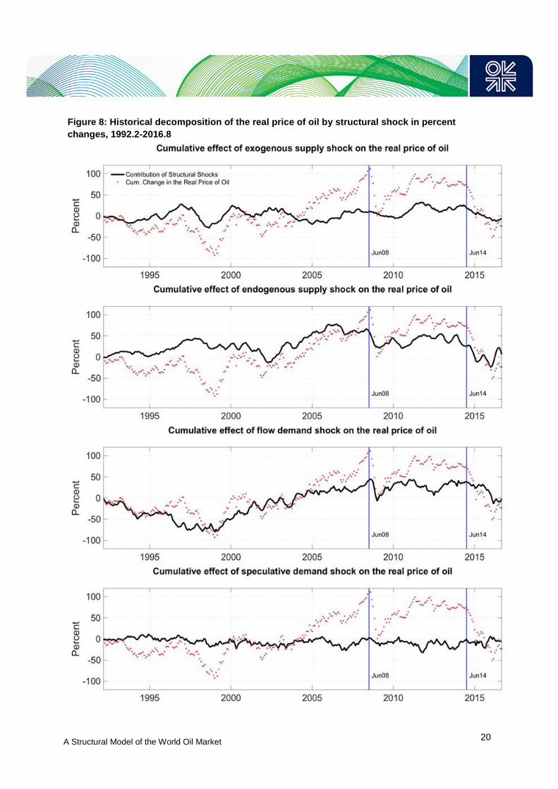
A Structural Model of the World Oil Market
20
Figure 8: Historical decomposition of the real price of oil by structural shock in percent
changes, 1992.2-2016.8

A Structural Model of the World Oil Market
21
4.2. Historical decomposition of the real price of oil
Figure 8 shows the historical decomposition of the real price of oil from February 1992 to August
2016. Each panel in the figure plots the respective cumulative contribution of each structural shock to
the real price of oil over time. The solid lines show how the real price of oil would have evolved, if all
structural shocks but the shock in question had been turned off. The dashed lines show the
cumulative change in the real price of oil caused by all structural shocks. The first panel indicates that
exogenous oil supply shocks overall made little contribution to the real price of oil, especially after
2000. By far the biggest contribution is due to the endogenous oil supply shock and the flow demand
shock. Endogenous oil supply shocks exerted significant upward pressure on the real price of oil
between 2004 and mid-2007, while their increasing importance to the market imbalance that plunged
the price of oil in June 2014 appears as early as mid-2012. Flow demand shocks are responsible for
the bulk of the oil price collapse in 1997-1999 and largely for the price surge that preceded up to June
2008, but there is little evidence to suggest that the 2014 oil price collapse was demand-driven. To
the extent that flow demand shocks mattered for the oil price slump of 2014-2016, they appear to be
responsible for a sharp defined decrease in the real price of oil only after mid-2015. The final panel
indicates that speculative demand shocks make no large systematic contribution to the evolution of
the real price of oil. Notwithstanding these historical decompositions, it is instructive to focus on
specific episodes since the early 2000s.
Figure 9 shows by how many dollars per barrel each oil supply and oil demand shock contributed to
the cumulative change in the real price of oil over some period of interest. The results are broken
down into three periods, representing: (a) the boom and bust of 2002-2009 (panel 1); (b) the oil price
recovery of 2009-2014 (panel 2); and (c) the oil price collapse of 2014-2016 (panel 3). The real price
of oil is inflation-adjusted in 2016.8 US dollars. The first five bars in each panel show the cumulative
contribution of each structural shock to the cumulative change in the real price of oil over the period in
question. The last bar indicates the actual cumulative change in the real price oil observed in the data.
Starting with the results from January 2002 to June 2008 in the first panel of Figure 9 (indicated by the
blue bars), we observe that out of the cumulative $119/b increase in the real price of oil over this
period, $50/b are attributed to the cumulative effect of the endogenous oil supply shocks and $48/b to
flow demand shocks. An additional $22/b are attributed to speculative and other demand shocks
combined. On the contrary, the cumulative effect of exogenous oil supply shocks is negative but
negligible, lowering the price of oil by $1/b. What these results merely suggest is that despite popular
belief that positive shifts in the flow demand for oil produced the bulk of the oil price surge between
2002-2008 (see Kilian, 2014, p. 6), if there was enough available production capacity to cover the
unexpected rise in flow demand, the real price of oil would have been lower by at least $50/b. This
does not mean that the oil price would not have increased close to $75/b (from $26/b) driven explicitly
by the growth of flow demand for oil, but endogenous capacity constraints in oil-producing countries
amplified the effect of flow demand shocks on the real price of oil roughly by 104%. The same can be
said for the subsequent plunge of the real price of oil by $96/b, between June 2008 and February
2009 (indicated by the grey bars in the first panel). Endogenous supply shocks in conjunction with
flow demand shocks accounted in total for 70% of the observed cumulative oil price decline, that is for
$36/b and $32/b respectively. The difference in this episode is that OPEC oil producers were able
(and willing) to adjust production to counterbalance the fall in flow demand and hence to smooth out
the price collapse, which proved to be short-lived.

A Structural Model of the World Oil Market
22
Figure 9: Contribution to the cumulative change in the real price of oil by structural shock, in
2016.8 USD per barrel

A Structural Model of the World Oil Market
23
The second panel in Figure 9 focuses on the oil price recovery between February 2009 and June
2014 (indicated by the blue bars). We observe that out of the cumulative $64/b increase in the real
price of oil over this period, $30/b are attributed to the cumulative effect of flow demand shocks and
$16/b are due to exogenous oil supply shocks following the outbreak of the 2011 Arab Uprisings.
Speculative demand shocks accounted for an additional $15/b, while endogenous supply shocks
accounted only for $4/b. It is useful to explore further the price dynamics over this period, especially
between June 2012 and June 2014 (indicated by the grey bars in the second panel). A closer
examination shows that even though the real price of oil was fairly balanced, associated with a minor
cumulative decline by $2/b, the underlying shocks in the oil market had been far more important. For
example, we observe that endogenous oil supply shocks in the form of unanticipated capacity
expansions exerted significant downward pressure on the real price of oil by $11/b. However, the real
price of oil response to these shocks have been small, as the excess supply was largely matched by
positive shifts in the flow demand for oil that accounted for $10/b of the cumulative price change.
These estimates contradict earlier conjectures in the literature suggesting that the market oversupply
at the time had been offset by unexpected exogenous shortfalls in crude oil production (see, for
example, Stevens & Hulbert, 2012). This explanation is not supported by our results. On the contrary,
out of the observed $16/b cumulative contribution of exogenous oil supply shocks to the price
increase between February 2009 to June 2014, these shocks account for at most $1/b after June
2012.
Finally, the third panel in Figure 9 shows that of the $64/b cumulative decline in the real price of oil
from June 2014 to January 2015 (indicated by the blue bars), $29/b are due to endogenous oil supply
shocks, $13/b are due to exogenous oil supply shocks and $12/b are attributed to flow demand
shocks. An additional $12/b to the price collapse are attributed to speculative demand shocks. These
estimates suggest that endogenous oil supply shocks alone roughly accounted for twice as much as
any other supply or demand shock in explaining the oil price plunge during this episode, indicating
that the persistence of the earlier capacity expansions were the dominant factor. On the contrary, an
unexpected slowdown in global real economic activity affecting the flow demand for oil was the major
contributor to a renewed price decline by $22/b between January 2015 to January 2016 (observed by
the grey bars in the third panel). Over this period, flow demand shocks accounted for an additional
cumulative decline in the real price of oil by $15/b, while endogenous oil supply shocks accounted
only for $1/b. The rest $6/b of the additional price drop was due to receding exogenous supply
disruptions. Thereafter, between January to August 2016 the real price of oil recovered from its earlier
drop by a cumulative increase of $14/b, of which over 95% is attributed to negative endogenous oil
supply shocks driven primarily by a contraction in US shale oil production (see Figure 10).
Figure 10: Contribution to the cumulative change in the real price of oil by structural shock
from January to August 2016, in 2016.8 USD per barrel

A Structural Model of the World Oil Market
24
An obvious question that arises from these results is why did flow demand for oil unexpectedly fail to
grow after June 2014, albeit a persistent decline in the real price of oil. Figure 11 illustrates how our
response estimates of real economic activity and the real price of oil to a positive endogenous oil
supply shock could help explain this paradox. We observe that whereas a positive endogenous oil
supply shock causes a persistent decline in the real oil price, this shock causes almost no change in
real economic activity on impact, followed by negative loops that progressively shift upwards (shown
by the trendline in the plot). These findings suggest that despite the belief that an oil price fall has a
net positive impact effect on global economy, the expected economic boost due to a market
oversupply is far from smooth (through its effect on price). This view is consistent with recent
empirical evidence in the literature suggesting that there appear no signs of economic growth picking
up in the first year following the price collapse not only in 2014, but also in 1986 (see IMF, 2015). Both
these episodes share two common and interrelated characteristics. First, a large persistent
component to the oil price declines. Second, a large loss in oil revenues for the oil exporters as a
response. Considering that oil exporting economies are heavily dependent on oil revenues and thus
they present many fiscal and external vulnerabilities, an expected lower oil price is associated with
adverse shocks to the economic growth of the oil exporters that pass-through to the global economy
(IMF, 2016).
Figure 11: Responses of global real economic activity and the real price of oil to a positive
endogenous oil supply shock
Notes: Both responses are expressed in percentages.
For example, Obstfeld, Arezki and Milesi-Ferretti (2016) argue that the oil exporting countries were
the largest contributors to the slowdown of global economic growth during 2015-2016, despite their
relatively small share of global GDP (about 15% based on purchasing power parity). In support to this
evidence the European Central Bank (2016) finds that the oil exporting economies experienced
substantial fiscal deficits, higher inflationary pressures and financial strains insofar as they exceeded
the marginal consumption gains in oil importing countries, resulting to a net negative impact on the
global economy. Furthermore, the absence of a balancing mechanism in the oil market (i.e. the
unwillingness of OPEC producers to cut output) has led to a prolonged environment of higher price
uncertainty that prompted oil producers to curtail capital investment in the upstream sector, weighing
heavily on global economic activity and trade as a response. For example, Baumeister and Kilian
(2017) show that because of the increased weight of oil-related investment in US real GDP growth
due to the shale oil boom, the sharp decline in capital expenditure in the shale oil sector dampened
the aggregate growth of the US economy. These examples highlight that the timing of the boost to

A Structural Model of the World Oil Market
25
global economic activity amid a market oversupply (through its effect on price), depends on whether
the latter is temporary or persistent. If temporary, oil exporters can draw on their financial reserves or
increase borrowing to buffer their losses in oil rents, while upstream investment will remain robust as
the oil price would be expected to recover. If persistent, the spending patterns of the oil exporters
need time to adjust, while upstream investment will diminish once the expected price exceeds the
long-run marginal cost of oil production, leading to a vulnerable macroeconomic environment and
abrupt shocks to the flow demand for oil in both directions (see Figure 11).20
As part of our sensitivity analysis, we address any concerns on whether our core conclusions are
sensitive to allowing for the possibility of lower price elasticities of oil demand in use. Table 2 presents
the minimum and maximum contribution of each structural shock based on all admissible models
within a pre-specified range of this elasticity, over some period of interest. The resulting estimates are
expressed in percent contribution of the total cumulative price change and they are rounded to the
nearest integer. Table 2 indicates that regardless of the sample period, the endogenous supply shock
and the flow demand shock account for the lion’s share of the cumulative change in the real price of
oil with only small quantitative differences across the elasticity ranges. For example, consider the
results for the period January 2002 to June 2008. Regardless of the elasticity range, endogenous oil
supply shocks accounted for anywhere between 34% and 49% of the cumulative price increase over
this period, while flow demand shocks accounted for anywhere between 33% and 49%. The rest
structural shocks combined accounted for anywhere between -3% and 30%. Likewise, regardless of
the elasticity range, these two shocks combined accounted for anywhere between 67% and 79% of
the cumulative price decline over June 2008 to January 2016, compared to the rest structural shocks
that combined accounted for anywhere between 14% and 38%. These estimates imply that our main
results are equally consistent regardless the choice of the admissible model.
Table 2: Minimum and maximum cumulative contribution to the real price of oil per range of
price elasticity of oil demand in use, in percentages
Evaluation
Period
Elasticity
in use
Exogenous
supply
shock
Endogenous
supply shock
Flow
demand
shock
Speculative
demand
shock
Other
demand
shock
2002.1 to
2008.6
[-0.30, 0] [-2, 11] [34, 47] [33, 44] [1, 13] [-1, 4]
[-0.25, 0] [-2, 13] [36, 49] [37, 47] [1, 13] [-2, 2]
[-0.20, 0] [ 0, 13] [36, 48] [37, 48] [1, 13] [-1, 2]
[-0.15, 0] [ 1, 13] [40, 48] [37, 49] [1, 11] [-2, 3]
2008.6 to
2016.1
[-0.30, 0] [12, 19] [37, 41] [32, 36] [-2, 1] [8, 11]
[-0.25, 0] [16, 18] [38, 41] [32, 38] [-5, 6] [8, 12]
[-0.20, 0] [16, 18] [37, 41] [30, 34] [-6, 7] [8, 12]
[-0.15, 0] [16, 18] [38, 41] [31, 34] [-6, 7] [8, 12]
4.3. Empirical comparison with a structural VAR model of flow supply, flow demand and speculative demand shocks
A central objective in this paper is to explore how the use of endogenous and exogenous supply
shock measures potentially affects the conventional estimates of the effects of supply and demand
shocks to the real price of oil obtained from structural oil market models that identify shocks to the
flow supply of oil collectively (see Section 2.1). This section compares our baseline results to those
obtained by re-estimating a structural VAR model of flow supply, flow demand and speculative
20 It is worth emphasising that shale oil production is widely perceived as being more price sensitive than conventional
production and thus shale oil investment is supposed to be more responsive in the short-run. However, there is still no empirical
evidence to support this view which remains ambiguous.

A Structural Model of the World Oil Market
26
demand in the tradition of Kilian and Murphy (2014). The model includes four monthly variables: (1)
the percent change in global oil production; (2) the measure of global real economic activity due to
Kilian (2009a); (3) the real price of crude oil; (4) and the proxy for changes in global oil inventories.
Data on global oil production rely on monthly estimates as reported by the EIA, while the rest
variables have been defined in Section 3.1. The sample extends from February 1990 to August 2016.
The model is estimated recursively by least squares using 24 autoregressive lags and seasonal
dummies.
Table 3: Sign restrictions on impact responses in the 4-variable SVAR model
Flow supply shock Flow demand shock Speculative demand shock
Oil production – + + Real activity – + – Real price of oil + + + Inventories +
The structural shocks are identified based on a combination of sign restrictions and bounds on the
impact price elasticities of oil supply and oil demand, building on Kilian and Murphy (2014). Table 3
summarises the sign restrictions on the impact responses of the model variables to the four structural
shocks, outlined as follows.21 A negative shock to the flow supply of crude oil lowers oil production
and real economic activity on impact and raises the real price of oil. A positive flow demand shock
raises oil production, real economic activity and the real price of oil on impact. A positive speculative
demand shock in equilibrium raises oil production, oil inventories and the real price of oil, but lowers
real economic activity. These restrictions implicitly identify the fourth residual demand shock. In
addition, we impose the dynamic sign restriction that a negative flow supply shock does not lower the
real price of oil for the first twelve months. Finally, the model bounds the impact price elasticity of oil
supply by 0.02 and the impact price elasticity of oil demand in use between -0.8 and 0. To facilitate
our comparison, we report the results for the model that yields an impact price elasticity of oil demand
in use closest to -0.29 (henceforth referred to as 4-variable SVAR), in line with the benchmark
elasticity estimate obtained by our baseline model. The response estimates of each model variable to
each structural shock are shown in Appendix A.
4.3.1. Responses of the real price of oil to oil supply and oil demand shocks
Figure 12 compares the responses of the real price of oil to each structural shock by model
specification. All shocks have been normalised as to imply an increase in the real price of oil. For
expository purposes, we also plot the aggregate oil price response to an exogenous and endogenous
supply shock referred to as total supply shock. It can be shown that a flow supply disruption causes a
temporary increase in the real price of oil that peaks after one year and then gradually starts to
decline towards its starting value. This pattern is qualitatively (and even quantitatively) similar to the
response of the real price of oil to an exogenous supply disruption, while it largely contrasts with the
oil price responses to a negative endogenous supply shock and a negative total supply shock. The
latter shock causes a steep and very significant increase in the real price of oil for the first six months
that despite its partial reversal after a year and a half, it remains persistent at all horizons. These
findings imply that flow supply shocks largely reflect disruptions in crude oil production that are
brought about by exogenous events, neglecting important information about endogenous innovations
to flow supply that arise within the crude oil market. We can observe that this missing information is
instead transmitted to the real price of oil through demand-related channels. In particular, the 4-
variable SVAR model attributes somewhat higher predictive power to the flow demand shock and the
speculative demand shock for the changes in the real price of oil, than the baseline model. Given
21 All structural shocks have been normalised as to imply an increase in the real price of oil. Missing entries in Table 3 denote
that no sign restrictions are imposed. For a detailed discussion see Kilian and Murphy (2014).

A Structural Model of the World Oil Market
27
these differences it is worth examining further the cumulative effect of each shock on the evolution of
the real price of oil by model specification.
Figure 12: Structural impulse responses of the real price of oil by model specification, in
percentages, 1990.2-2016.8
4.3.2. Contribution of the structural shocks to oil price movements since 2002
Figure 13 plots the cumulative change in the real price of oil caused by each structural shock over
January 2002 to August 2016, obtained from the 4-variable SVAR model (red bars) and the baseline
model (blue bars). The first bar in each panel compares the cumulative contribution of flow supply
shocks against that of total supply shocks, as specified in the previous section. It can be shown that
regardless of the period in question, the 4-variable SVAR model attributes the bulk of the cumulative
changes in the real price of oil to flow demand shocks, whereas the differences between the two
models regarding the speculative demand shock are quite small. For example, of the $119/b
cumulative increase in the real price of oil from January 2002 to June 2008 (first panel), this model
assigns $90/b to the cumulative effect of flow demand shocks compared to $48/b attributed by the
baseline model. Likewise, of the $99/b cumulative decline in the real price of oil from June 2008 to
August 2016 (second panel), the 4-variable SVAR model assigns $75/b to the cumulative effect of
flow demand shocks compared to the baseline model that assigns only $32/b to this shock. Evidently,
these differences operate at the expense of the explanatory ability of the supply determinant, as flow
supply shocks due to the 4-variable SVAR model are found to have played a limited role in explaining
the evolution of the real price, compared to the more significant role assigned to total supply shocks
due to the baseline model. The former assigns -$1/b and -$14/b to the cumulative contribution of flow
supply shocks to the price changes over the two periods, against $49/b and -$52/b assigned by the
baseline model to total supply shocks respectively.

A Structural Model of the World Oil Market
28
Figure 13: Contribution to the cumulative change in the real price of oil by structural shock, by
model specification, in 2016.8 USD per barrel
It is worth emphasising that the cumulative contribution of flow supply shocks is strikingly similar to
that of exogenous supply shocks, that is of -$1/b and -$12/b. These results underscore that the
traditional emphasis on changes in global oil production, per se, for modelling the supply-side of the
world oil market collectively is misplaced. Moreso, the claim that economic fundamentals in the form
of flow demand and to a lesser extent speculative demand have been the main determinants of the
real price of oil must be rethought. Much of the prima facie case against an important role of oil supply
shocks rests on the fact that the traditional shock measures of flow supply are informationally
inadequate. Whereas exogenous shocks to crude oil production are not negligible, endogenous
shocks in global production capacity have been a far more important determinant for major oil price
fluctuations in recent years.
4.3.3. Real-time forecasts of the Brent price as of June 2014
Given the differences between the two VAR models when it comes to the identification of the
structural shocks that drive the price of oil and the overall importance of oil supply and oil demand
shocks, it is useful to contrast their ability to predict the price of oil. This is an important test of the
validity of our core conclusions. Recent studies have shown that suitably chosen reduced-form VAR
models that include the key variables relevant to the determination of the real price of oil exhibit
superior out-of-sample forecast accuracy than alternative forecasting models (see Baumeister &
Kilian, 2012). Recall that a clear distinction between the competing forecasting models is that the
baseline model decomposes the oil supply determinant into its distinct exogenous and endogenous
components, whereas the 4-variable SVAR model does not. The question of interest is whether the
inclusion of the proposed decomposition of oil supply shocks in a forecasting model of the price of oil
potentially improves the real-time predictive accuracy of conventional VAR forecasts that model

A Structural Model of the World Oil Market
29
shocks to the flow supply of oil collectively. This question may be addressed by generating real-time
forecasts of the Brent price using the reduced-form representation of each structural VAR model
(Baumeister & Kilian, 2014). The objective is to assess the real-time forecasting performance of each
model in predicting the June 2014 oil price collapse and the subsequent evolution of the Brent price
up to December 2016, converted to nominal US dollars.
Figure 14: One-step ahead forecasts of the Brent price for July 2014 to January 2015, in
nominal USD per barrel, 2014.1-2015.1
Figure 14 shows the evolution of the nominal Brent price from January 2014 to January 2015, along
with the real-time forecasts obtained by the 4-variable SVAR model and the baseline model as of
June 2014 (marked by the vertical line in the plot). For expository purposes, we focus on the one-step
ahead forecasts. Each forecast is generated in real-time using only information as of the previous
month (denoted by the black markers). As can be seen from Figure 14, the 4-variable SVAR model
forecasts perform relatively poorly in predicting the one-step ahead directional change of the Brent
price, with a success ratio of 43% (i.e. the fraction of times that the model correctly predicts the
directional change of the oil price). Even though the forecasts in July and August are very close to the
actual Brent price, the model systematically overpredicts the price of oil from the September forecast
onwards by about $13/b. On the contrary, the baseline model forecasts are much closer to the
realisations of the Brent price, with a success ratio of 86%. Only the September 2014 and January
2015 baseline forecasts overpredict the Brent price by a more significant amount of $7/b and $10/b
respectively. The consistency of this pattern, regardless of the model specification, raises the
question of what are the causes of the competing forecast errors after August 2014, in the related
context of supply and demand shocks to the price of oil.

A Structural Model of the World Oil Market
30
Figure 15: One-step ahead forecast errors from September 2014 to January 2015
Notes: The forecast errors corresponding to the shock measures of crude oil supply due to the baseline model, are normalised as to reflect the aggregate forecast errors in global oil production.
Figure 15 traces the one-step ahead forecast errors by model specification from September 2014 to
January 2015, for the Brent price, for global oil production, for global real economic activity and for
changes in oil inventories. The first entry in each of the bar charts, corresponding to the errors in
forecasting September 2014, shows large differences between the forecast errors of the two VAR
models for global oil production and for oil inventories. The forecast errors for global real economic
activity are largely in agreement in all months. The September forecast due to the 4-variable SVAR
model generated a very large positive forecast error for global oil production (corresponding to about
3% of world oil output), which is lower by almost two-thirds due to the baseline model (corresponding
to 1.2% of world oil output). The latter also attributed a small but non-negligible positive forecast error
for the change in oil inventories (corresponding to 0.9% of OECD industry oil stocks). Thereafter, with
the benefit of an additional month of information the one-step ahead forecast errors for the Brent price
due to the 4-variable SVAR model persist well into October and November, while the errors due to the
baseline model in the same months are largely corrected for. Considering that there are no large
forecast errors associated with either an unexpectedly large supply or demand shock, a strong case
can be made for the persistence of the forecast errors due to the 4-variable SVAR model being
associated with the absence of critical information pertaining to the sequence of the earlier
endogenous supply shocks. Likewise, despite both December forecasts attributing the forecast errors
for the Brent price to large negative forecast errors for global real economic activity (compared with
the actual index value of global real economic activity shown in Appendix B), the baseline forecast
corrected this error by about one third at the expense of a large positive forecast error for global oil
production (corresponding to about 1.5% of world oil output). Over 90% of the latter forecast error is

A Structural Model of the World Oil Market
31
attributed to endogenous factors, due to the baseline model, which again appears to drive the
mismatch between the January 2015 forecasts.
Figure 16: Real-time forecasts of the Brent price as of December 2014, in nominal USD per
barrel, 2013.12-2016.12
In order to fully appreciate the implications of the informational inadequacy of flow supply shock
measures at longer horizons, Figure 16 shows the evolution of the Brent price from December 2013
to December 2016 together with the real-time forecasts of the Brent price by model specification as of
December 2014 (marked by the vertical line in the plot). Very similar results hold for both models
regarding the directional accuracy of the December forecasts 24-months ahead, with a success ratio
of 54% due to the 4-variable SVAR forecast and 50% due to the baseline forecast. However, by
comparison, the baseline model forecast produced systematically lower real-time mean squared
prediction errors (MSPEs), denoting higher predictive accuracy (Table 4). In most cases, MSPE
reductions are higher than 40% relative to the 4-variable SVAR model forecast even at longer
horizons.
Table 4: Recursive MSPE ratio of the baseline model forecast relative to the 4-variable SVAR
model forecast
Month
[Horizon]
Jan 15
[1]
Mar 15
[3]
Jun 15
[6]
Sep 15
[9]
Dec 15
[12]
Jun 16
[18]
Dec 16
[24]
MSPE 0.4043 0.4535 1.0587 0.6560 0.5781 0.5785 0.4437
Notes: Boldface indicates improvements relative to the 4-variable SVAR model forecast.
An intuitive way to put these results into perspective is to observe the bar charts in Figure 17 that
compare the actual and predicted annual change of the key oil market indicators in 2015 and 2016,
based on the real-time forecasts as of December 2014. Evidently, the main disagreement between
the competing real-time forecasts is associated with the predicted annual growth of global oil
production. On the one hand, the real-time 4-variable SVAR forecast predicted that global oil
production in 2015 will marginally turn negative by -0.15 mb/d on average, before declining further in
2016 by -0.62 mb/d year-over-year (y-o-y). On the other hand, the real-time baseline forecast

A Structural Model of the World Oil Market
32
correctly predicted that the annual growth of global oil production will persist well into 2015 and 2016,
by 1.6 mb/d and 1.3 mb/d y-o-y, missing the average 2016 realisation only by 0.59 mb/d. As a result,
in 2016, the 4-variable SVAR forecast predicted that the Brent price would rise at $88/b year-end
compared to $53/b of the actual December price, whereas the baseline forecast predicted a price
ceiling at $66/b by the second half of the year (see Figure 16). These results are particularly
informative given that the ability of the baseline forecasting model to distinguish between oil supply
shocks that are different in nature has led to the much closer realisations of global oil production and
hence of the Brent price over time. In support to the robustness of the baseline forecasting model, is
also the fact that both forecasts detected an unexpected weakening of global economy and a stronger
than expected growth of storage demand for oil.
Figure 17: Actual and predicted annual change of the key oil market indicators for 2015 and
2016, year-over-year
5. Conclusion
A recurring question in recent and past episodes of the crude oil market is how important are oil
supply and oil demand shocks in explaining major oil price fluctuations. Advancements in theoretical
and empirical work during the past decade made considerable strides addressing this question,
enhancing our understanding of the determinants of oil price shocks. The conventional view today is
that most major oil price shocks are explained by oil demand shocks collectively, rather than flow
supply shocks, with a central role played by shifts in the global business cycle affecting the flow
demand for oil. Traditionally, flow supply shocks were thought to reflect disruptions in crude oil
production triggered by geopolitical events in oil producing countries and politically motivated OPEC
decisions, both of which occurred outside the confines of the crude oil market. However, such
exogenous shocks to global crude oil production constitute only but one type of oil supply shock.

A Structural Model of the World Oil Market
33
There also may be shocks to global production capacity associated with the interaction of an array of
geological, economical, regulatory and technological factors that combined can affect the supply of
oil. This type of oil supply shocks arises endogenously with respect to the crude oil market and
reflects the rate of investment to new production capacity and the lead times in bringing new capacity,
conditional on the expectations of oil producers about future market conditions and expected price.
This means that oil price shocks can only be understood with the help of structural models of the
world oil market that jointly identify and estimate the exogenous and endogenous supply components
in the real price of oil, along the components driven by flow demand and speculative demand. In this
paper, we augmented the structural VAR model of flow supply, flow demand and speculative demand
to allow for the decomposition of the supply determinant based on some novel approaches that in turn
allow for the simultaneous identification of all four types of supply and demand shocks conditional on
all past data.
There are two reasons why this decomposition is important. One is the fact that much of the prima
facie case against an important role of oil supply shocks in explaining the evolution of the real price of
oil rests on traditional measures of flow supply that are informationally inadequate. Our findings
suggest that flow supply shocks largely reflect disruptions in crude oil production that are brought
about by exogenous events, neglecting important information about endogenous innovations to flow
supply that arise within the crude oil market. This missing information is instead transmitted to the real
price of oil through demand-related channels at the expense of the explanatory power of the supply
determinant. The second is that the relative importance of oil supply shocks for the real price of oil
differs greatly, depending on the nature of the shock. For example, endogenous oil supply shocks
appear to be associated with a markedly larger and more persistent impact on the real price of oil
than exogenous disruptions in crude oil production. Furthermore, these shocks are also associated
with important indirect effects on the real price of oil through other demand-related channels, such as
their asymmetric impact effect on global economy.
The central message of the paper is that while there is overwhelming empirical evidence in the
literature that most large and persistent fluctuations in the real price of oil have been driven by the
cumulative effects of oil demand, the robustness of this evidence crucially depends on the rigorous
identification of oil supply shocks. In general, our analysis showed that most large and persistent
fluctuations in the real price of oil since the early-1990s can be explained either by large positive shifts
in flow demand confronted by negative endogenous oil supply shocks or by persistent positive
endogenous oil supply shocks confronted by unexpected negative shifts in the flow demand for oil.
For example, our results suggest that despite the popular belief in the literature that the sustained run-
up in the real price of oil between 2002-2008 was caused primarily by positive shifts in the global
business cycle affecting oil demand, endogenous capacity constraints in oil-producing countries more
than doubled the impact effect of flow demand shocks to the real price of oil. Likewise, while the 2014
oil price collapse was primarily triggered by the persistence of positive endogenous oil supply shocks,
an unexpected downshift of the global business cycle in mid-2015 aggravated the recent price
downcycle both in terms of magnitude and duration. On the contrary, there is little evidence to
suggest that exogenous supply disruptions and shifts in speculative demand for oil contributed much
to the evolution of the real price of oil over the sample period, confirming some of the core
conclusions of earlier studies. Notwithstanding, both these shocks remain important components for
the structural decomposition of the real price of oil. Finally, we demonstrated that forecasting models
able to distinguish between oil supply shocks that are different in nature, produce more realistic out-
of-sample estimates of the sequences of supply and demand shocks, thus enjoying higher real-time
predictive accuracy than forecasting models that incorporate shocks to the flow supply of oil
collectively. These findings underscore the importance of explicitly modelling endogenous supply
shocks in structural models of the world oil market and the central role of production capacity
pressures in understanding the evolution of the real price of oil.

A Structural Model of the World Oil Market
34
Acknowledgments
The authors are overly grateful to Lutz Kilian for useful insights and expertise that greatly assisted the
research.

A Structural Model of the World Oil Market
35
References
Adelman, M. A. 1993. Modelling World Oil Supply. The Energy Journal 14(1): 1-32.
Adelman, M. A. 2002. World Oil Production and Prices: 1947–2000. The Quarterly Review of
Economics and Finance, 42(2): 169-191.
Adelman, M. A. and Watkins, G. C. 2008. Reserve Prices and Mineral Resource Theory. The Energy
Journal, 29(2008): 1-16.
Alquist, R. and Guenétte, J. D. 2014. A Blessing in Disguise: The Implications of High Global Oil
Prices for the North American Market. Energy Policy, 64(C): 49-57.
Alquist, R. and Kilian, L. 2010. What Do We Learn from the Price of Crude Oil Futures? Journal of
Applied Econometrics, 25(4): 539-573.
Alquist, R., Kilian, L. and Vigfusson, R. J. 2013. Forecasting the Price of Oil. In G. Elliot and A.
Timmersmann (ed.) Handbook of Economic Forecasting, 2: 427-507. Amsterdam: North Holland.
Arezki, R. 2016. Seven Questions on Rethinking the Oil Market in the Aftermath of the 2014-16 Price
Slump. IMF Research Bulletin, 17(3): 9-12.
Arezki, R. and Blanchard, O. 2015. The 2014 Oil Price Slump: Seven Key Questions. IMF Direct,
International Monetary Fund: December 22.
Babel, A. and McGillicuddy, J. 2015. Oil Prices: Is Supply or Demand Behind the Slump? Federal
Reserve Bank of St. Louis.
Baffes, J., Kose, M. A., Ohnsorge, F. and Stocker, M. 2015. The Great Plunge in Oil Prices: Causes,
Consequences and Policy Responses. Policy Research Note, No. 1 World Bank.
Barsky, R. B. and Kilian, L. 2002. Do We Really Know that Oil Caused the Great Stagflation? A
Monetary Alternative. In B.S. Bernanke and K. Rogoff (ed.) NBER Macroeconomics Annual 2001, 16:
137-183. Cambridge: MIT Press.
Barsky, R. B. and Kilian, L. 2004. Oil and the Macroeconomy since the 1970s. Journal of Economic
Perspectives, 18(4): 115-134.
Baumeister, C. and Hamilton, J. D. 2015. Structural Interpretation of Vector Autoregressions with
Incomplete Identification: Revisiting the Role of Oil Supply and Oil Demand Shocks. Manuscript
University of Notre Dame and UCSD.
Baumeister, C. and Kilian, L. 2012. Real-Time Forecasts of the Real Price of Oil. Journal of Business
and Economic Statistics, 30: 326-336.
Baumeister, C. and Kilian, L. 2014. Real-Time Analysis of Oil Price Risks using Forecast Scenarios.
IMF Economic Review, 62: 119-145.
Baumeister, C. and Kilian, L. 2016a. Forty Years of Oil Price Fluctuations: Why the Price of Oil May
Still Surprise Us. Journal of Economic Perspectives, 30(1): 139-160.
Baumeister, C. and Kilian, L. 2016b. Understanding the Decline in the Price of Oil since June 2014.
Journal of the Association of Environmental and Resource Economics, 3(1): 131-158.
Baumeister, C. and Kilian, L. 2017. Lower Oil Prices and the U.S. Economy: Is This Time Different?
Brookings Papers on Economic Activity, Fall 2016: 287-336.
Baumeister, C. and Peersman, G. 2013a. The Role of Time-Varying Price Elasticities in Accounting
for Volatility Changes in the Crude Oil Market. Journal of Applied Econometrics, 28(7): 1087-1109.

A Structural Model of the World Oil Market
36
Baumeister, C. and Peersman, G. 2013b. Time-Varying Effects of Oil Supply Shocks on the US
Economy. American Economic Journal: Macroeconomics, 5(4): 1-28.
Bodenstein, M., Erceg, C. J. and Guerrieri, L. 2007. Oil Shocks and External Adjustment. International
Finance Discussion, No. 897.
Caldara, D., Cavallo, M. and Iacoviello M. M. 2016. Oil Price Elasticities and Oil Price Fluctuations.
FRB International Finance Discussion Paper, No. 1173.
Canova, F. and De Nicolo, G. 2002. Monetary Disturbances Matter for Business Cycle Fluctuations in
the G-7. Journal of Monetary Economics, 49: 1131-1159.
Dotsey, M. and Reid, M. 1992. Oil Shocks, Monetary Policy, and Economic Activity. FRB Richmond
Economic Review, 78(4): 14-27.
Economou, A. 2016. Oil Price Shocks: A Measure of the Exogenous and Endogenous Supply Shocks
of Crude Oil. Oxford Institute for Energy Studies WPM 68.
European Central Bank. 2016. Economic and Monetary Developments. Economic Bulletin Issue, No.
4/2016: June.
Fattouh, B. 2006. Spare Capacity and Oil Price Dynamics. Middle East Economic Survey XLIX(5).
Fattouh, B. 2007a. The Drivers of Oil Prices: The Usefulness and Limitations of Non-Structural
Models, Supply-Demand Frameworks, and Informal Approaches. EIB papers, 12(1): 128-156.
Fattouh, B. 2007b. OPEC Pricing Power: The Need for a New Perspective. Oxford Institute for Energy
Studies WPM 31.
Fattouh, B. and Mabro, R. 2006. The Investment Challenge. In R. Mabro (ed.) Oil in the 21st Century:
Issues, Challenges and Opportunities, 101-127. Oxford: Oxford University Press.
Fattouh, B. and Mahadeva, L. 2013. OPEC: What Difference Has It Made? Oxford Institute for Energy
Studies MEP 3.
Fattouh, B. and Sen, A. 2015. Saudi Arabia Oil Policy: More than Meets the Eye? Oxford Institute for
Energy Studies MEP 13.
Fattouh, B., Kilian, L. and Mahadeva, L. 2012. The Role of Speculation in Oil Markets: What Have We
Learned So Far? Oxford Institute for Energy Studies WPM 45.
Faust, J. 1998. On the Robustness of Identified VAR Conclusions about Money. Carnegie-Rochester
Conference Series on Public Policy, 49: 207-244.
Favero, C. A. and Perasan M. H. 1991. Oil Investment in the North Sea. Oxford Institute for Energy
Studies WP EE15.
Gately, D. 2011. OPEC at 50: Looking Back and Looking Ahead. In conference at the National Energy
Policy Institute: April 18.
Gately, D., Adelman, M. A. and Griffin, J. M. 1986. Lessons from the 1986 Oil Price Collapse.
Brookings Papers on Economic Activity, 2(1986): 237-284.
Hamilton, J. D. 1983. Oil and the macroeconomy since World War II. Journal of Political Economy,
91:228-248.
Hamilton, J. D. 1985. Historical causes of postwar oil shocks and recessions. Energy Journal, 6: 97-
116.
Hamilton, J. D. 2003. What Is an Oil Shock? Journal of Econometrics, (113): 363-398.
Hamilton, J. D. 2009a. Understanding Crude Oil Prices. The Energy Journal, 30(2): 179-206.

A Structural Model of the World Oil Market
37
Hamilton, J. D. 2009b. Causes and Consequences of the Oil Shock of 2007-08. Brooking Papers on
Economic Activity, Spring: 215-259.
Hamilton, J. D. 2013a. Historical Oil Shocks. In Routledge Handbook of Major Events in Economic
History: 239-265. edited by Randall E. Parker and Robert Whaples. New York: Routledge Taylor and
Francis Group.
Hamilton, J. D. 2013b. Oil Prices, Exhaustible Resources, and Economic Growth. In Handbook of
Energy and Climate Change: 29-57. edited by Roger Fouquet. Cheltenham: Edward Elgar Publishing.
Hamilton, J. D. 2014. The Changing Face of Crude Oil Markets. IAEE Energy Forum, 4th Quarter: 7-
13.
Hamilton, J. D. and Herrera, A. M. 2004. Oil Shocks and Aggregate Macroeconomic Behavior: The
Role of Monetary Policy. Journal of Money, Credit, and Banking, 36: 265-286.
Hoover, K. D. and Perez, S. J. 1994. Post Hoc Ergo Propter Hoc Once More: An Evaluation of ‘Does
Monetary Policy Matter?’ in the Spirit of James Tobin. Journal of Monetary Economics, 34(1994): 89-
99.
Inoue, A. and Kilian, L. 2013. Inference on Impulse Response Functions in Structural VAR Models.
Journal of Econometrics, 177: 1-13.
International Monetary Fund. 2015. Global Implications of Lower Oil Prices, IMF Staff Discussion
SDN/15/15.
International Monetary Fund. 2016. Economic Diversification in Oil-Exporting Arab Countries. In
Annual Meeting of Arab Ministers of Finance: April.
Katzman, K. 2003. Iraq: Oil-For-Food Program, International Sanctions, and Illicit Trade.
Congressional Research Service: April 16.
Kaufmann, R. K. 2011. The Role of Market Fundamentals and Speculation in Recent Price Changes
for Crude Oil. Energy Policy, 39(1): 105-115.
Kilian, L. 2006. Not All Oil Price Shocks Are Alike: Disentangling Demand and Supply Shocks in the
Crude Oil Market. CEPR Discussion Paper No. 5994.
Kilian, L. 2008a. The Economic Effects of Energy Price Shocks. Journal of Economic Literature,
46(4): 871-909.
Kilian, L. 2008b. Exogenous Oil Supply Shocks: How Big Are They and How Much Do They Matter for
The U.S. Economy? Review of Economics and Statistics, 90(2): 216-240.
Kilian, L. 2009a. Not All Oil Price Shocks Are Alike: Disentangling Demand and Supply Shocks in the
Crude Oil Market. American Economic Review, 99(3): 1053-1069.
Kilian, L. 2009b. Comment on "Causes and Consequences of the Oil Shock of 2007-08" by James D.
Hamilton. Brookings Papers on Economic Activity, 1(2009): 267-278.
Kilian, L. 2014. Oil Price Shocks: Causes and Consequences. Annual Review of Resource
Economics, 6(2014): 133-154.
Kilian, L. and Hicks, B. 2013. Did Unexpectedly Strong Economic Growth Cause the Oil Price Shock
of 2003-2008? Journal of Forecasting, 32(5): 385-394.
Kilian, L. and Lee, T. 2014. Quantifying the Speculative Component in the Real Price of Oil: The Role
of Global Oil Inventories. Journal of International Money and Finance, 42: 71-87.
Kilian, L. and Lütkepohl, H. 2017. Structural Vector Autoregressive Analysis. Forthcoming: Cambridge
University Press.

A Structural Model of the World Oil Market
38
Kilian, L. and Murphy, D. 2012. Why Agnostic Sign Restrictions Are Not Enough: Understanding the
Dynamics of Oil Market VAR Models. Journal of the European Economic Association, 10(5): 1166-
1188.
Kilian, L. and Murphy, D. 2014. The Role of Inventories and Speculative Trading in the Global Market
for Crude Oil. Journal of Applied Econometrics, 29(3): 454-478.
Knittel, R. C. and Pindyck, R. S. 2013. The Simple Economics of Commodity Price Speculation.
NBER Working Paper 18951.
Lippi, F. and Nobili, A. 2009. Oil and the Macroeconomy: A Quantitative Structural Analysis. Bank of
Italy: Discussion Paper: 704.
Lombardi, M. and Van-Robays, I. 2011. Do Financial Investors Destabilise the Oil Price? ECB
Working Paper Series, No. 1253/October 2010.
Mabro, R. 1992. OPEC and the Price of Oil. The Energy Journal, 13(2): 1-17.
Mabro, R. 1998. The Oil Price Crisis of 1998. Oxford Institute for Energy Studies SP 10.
Mabro, R. 2006. Oil in the 21st Century: Issues, Challenges and Opportunities. Oxford: Oxford
University Press.
McNally, R. 2012. Managing Oil Market Disruption in a Confrontation with Iran. Council on Foreign
Relations Energy Brief January.
Melolinna, M. 2012. Macroeconomic Shocks in an Oil Market VAR. ECB Working Paper Series, No.
1432/May 2012.
Naimi, A. 2005. Shaping the Energy Future: The Role of Saudi Arabia. Middle East Economic Survey
XLVIII(40).
Nakov, A. and Pescatori, A. 2010. Monetary Policy Trade-Offs with a Dominant Oil Producer. Journal
of Money, Credit and Banking, 42(1).
Obstfeld, M., Arezki, R. and Milesi-Ferretti G. M. 2016. Oil Prices and the Global Economy: It’s
Complicated. VoxEU: April 13.
Pindyck, R. S. 1991. Irreversibility, Uncertainty and Investment. Journal of Economic Literature, 29(3):
1110-1148.
Sandrea, I. 2014. US Shale Gas and Tight Oil Industry Performance: Challenges and Opportunities.
Oxford Institute for Energy Studies: Energy Comment.
Smith, J. L. 2009. World Oil: Market or Mayhem. Journal of Economic Perspectives, 23(3): 145-164.
Smith, J. L. 2012. On the Portents of Peak Oil (And Other Indicators of Resource Scarcity). Energy
Policy 44: 68-78.
Stevens, P. 2015. The Shale Technology Revolution and the Implications for the GCC. Arab Center
for Research and Policy Studies: January.
Stevens, P. and Hulbert, M. 2012. Oil Prices: Energy Investment, Political Stability in the Exporting
Countries and OPEC’s Dilemma. EEDP Programme Paper, No. 2012/03.
Uhlig, H. 2005. What Are the Effects of Monetary Policy on Output? Results from an Agnostic
Identification Problem. Journal of Monetary Economics, 52: 381-419.

A Structural Model of the World Oil Market
39
Appendix A
Figure A1: Structural impulse responses and corresponding pointwise 68% posterior error
bands conditional on the estimate of the 4-variable SVAR model, 1990.2-2016.8
Notes: All structural shocks have been normalised as to imply an increase in the real price of oil. All responses but the inventory responses are expressed in percentages. The inventory responses are in million barrels.
A Structural Model of the World Oil Market
40
Appendix B
Figure B1: Index of global real economic activity in percent deviations from trend, 2014.1-
2015.1
Notes: This index is developed in Kilian (2009a) and is designed to measure the state of global economy. Negative index values represent recessionary phases of the economy and positive values expansionary phases. For a meaningful interpretation of the indicator, the magnitude of the deviations from zero should only be viewed in relation to the past.