A Stochastic Stormwater Quality Volume-SizingMethod with First Flush Emphasis

Soroosh Sharifi1, Arash Massoudieh2*, Masoud Kayhanian3

ABSTRACT: A Monte Carlo simulation technique was applied toassess the effect of stormwater quality volume captured by bestmanagement practices (BMPs) on the frequency of dischargingconcentrations of constituents above certain designated threshold limits.The method used an assumption of a power law relationship between thecumulative load and flow to incorporate the first flush effect. Theexponent of this relationship was considered a random variable and itsfrequency distribution was obtained from 78 measured pollutographsfrom three urban highway sites in West Los Angeles, California.Although the effect of rain depth captured by BMPs is site-specific, themethod offered here provides a systematic approach to evaluate theeffect of selecting various regulatory guidelines for controlling urbanstormwater pollution on the overall discharge of pollutants intowaterways. This allows selecting the requirements for capturing runoffvolume by BMPs based on the tradeoff between the probability ofconcentration criteria violation and economic factors. Water Environ.Res., 83, 2025 (2011).

KEYWORDS: best management practices, water quality volume,stormwater, total maximum daily load, first flush.

doi:10.2175/106143011X12989211

IntroductionNonpoint sources of pollution generated from urban storm-

water runoff are now deemed to be significant contributors ofpollutants in waterbodies (Barrett et al., 1998; Horan, 1990;Larsen et al., 1998). This has led to the development ofregulatory guidelines (e.g., RIDEM and CRMC, 2010; MPCA,2008; NHDES, 2008; U.S. EPA, 2004) aimed at controlling orreducing the effect of non-point-source pollutants to receivingwaters. These regulations mainly rely on development of bestmanagement practices (BMPs) to treat nonpoint sources or toreduce the direct discharge of polluted water into receivingwaters. These BMPs can primarily be categorized into twogroups: (1) methods that reduce the discharge of water intosurface waterbodies by promoting infiltration into the ground orstore the water so that it is never released in the form of surfacerunoff, such as through the use of infiltration ponds (Jefferies etal., 1999), rain gardens (Davis, 2008), rain barrels (MPCA, 2008),and permeable pavements (Balades et al., 1995); and (2) methodsthat remove particulate matter and the contaminants bound tothem and, sometimes, nutrients through burial or denitrification.

These include methods such as retention, detention (England,2001), bioretention basins (Hsieh and Davis, 2005), sand filters(MassDEP, 1997), and constructed wetlands (Ahlfeld andMinihane, 2004; MassDEP, 1997; U.S. EPA, 2004). Theeffectiveness of most of these BMPs depends on the volume ofstorm runoff that can be captured and treated by them, which isdirectly related to the size of BMPs. The efficiency of BMPs alsodepends on whether they are able to entrap the most pollutedportion of the storm runoff by taking advantage of the concept offirst flush (Kayhanian and Stenstorm, 2005).

The term, first flush, was first introduced in the 1970s (Sartorand Boyd, 1972). The intuitive and general concept of first flushrefers to the release of the greater fraction of constituent mass orconcentration of pollutants at the early part of a storm event(Barco et al., 2008; Kim et al., 2005). This phenomenon wasthought to be caused by the quick wash-off of pollutantsaccumulated during dry weather periods on the pavementsurface. In general, significant factors affecting the occurrenceand severity of first flush in an event include storm character-istics, size and drainage characteristics of the drainage area, themobility and properties of pollutants, and the length of theantecedent dry period (Bertrand-Krajewski et al., 1998; Deletic,1998; Deng et al., 2005; Kang et al., 2008). Several attempts havebeen made to develop empirical (e.g., Deletic and Maksimovic1998; Gupta and Saul 1996) or physically based models (e.g.,Kang et al. 2006; Massoudieh et al. 2008) to predict the first flushbehavior in highway environments. Despite differences re-garding the quantitative definition of first flush (Deng et al.,2005) and the universality and transferability of the proposedpredictive models (Flint and Davis, 2007; Kang et al., 2006), theexpectation of a higher pollutant concentration at the beginningof the storm has been the basis of the most practiced criteria forthe design of stormwater treatment BMPs.

Various regulatory criteria have been suggested for thetreatment of captured water volume by BMPs, referred to aswater quality volume (WQV). The most widely presented andadopted rule is based on the first flush concept and requiresa fixed depth of runoff to be captured (also referred to as waterquality depth [WQD]) (e.g., MassDEP, 1997; MPCA, 2008). Forexample, many states throughout the United States adopt thehalf-inch rule, which requires the first one-half inch of runoff betreated by BMPs. However, because of regional variations ofprecipitation, a single WQD might not be adequate over anentire state (Chang et al., 1990). The alternative approachrequires capturing and treating a certain fraction of the rainvolume from each event. For example, the 90% rainfall eventcriterion, adopted by many states including Minnesota (MPCA,2008) and New Hampshire (NHDES, 2008), defines WQV as

1,2* Department of Civil Engineering, Catholic University of America,620 Michigan Ave. N.E., Washington, D.C. 20064; e-mail: massoudieh@cua.edu.3 Department of Civil and Environmental Engineering, University ofCalifornia Davis.

November 2011 2025

being equal to the storage required to capture and treat 90% ofthe entire rainfall volume for 24-hour design storms on anannual basis. The third approach requires a removal rate forpollutants often surrogated by the fraction of total suspendedsolids (TSS) removed from the runoff (U.S. EPA, 2004). Themost frequently used pollutant removal criterion requires an80% removal of TSS on an individual storm event basis (U.S.EPA, 2004; MPCA, 2008).

Despite their limitations (Chang et al., 1990), first flush-basedsizing criteria are still widely used and valued for their relativesimplicity. For example, Sartor and Boyd (1972) assumed thatreductions in pollutants follow an exponential decay curve andproposed a sizing equation relating the magnitude of first flushto rainfall intensity and the particle size of the constituent.Furthermore, measuring the effects of roofing material on theturbidity of first harvested rainwater and the amount of firstflush and following a mass balance approach, Martinson andThomas (2005) proposed a simple rule-of-thumb for first flushbehavior that states that ‘‘for each [millimeter] of first flush, thecontaminate load will halve’’. Based on this rule, a rationalmethod was suggested for sizing some BMP devices based onfirst flush and the desired material intended to be removed.Attempts have also been made to define the flowrate thatcorresponds to the first flush runoff depth to optimize flow-through BMPs (Ahlfeld and Minihan, 2004; Froehlich, 2009).However, based on the authors’ knowledge, no quantitativesystematic approach for determining a WQD criterion has beenoffered that considers uncertainties in event characteristics andthe first flush behavior of pollutants during events. Researchpresented in this article extends previous work by proposinga probabilistic method for assessment of the effect of sizingcriteria on effluent water quality, which takes into account boththe uncertainties in first flush behavior during the events and theprecipitation pattern. A model based on traditional first flushformulations was developed and a Monte Carlo simulation wasperformed to estimate the number of times various water qualityconstituents in the effluent exceeded a predefined set of waterquality standards as a result of capturing various depths ofprecipitation. Although the proposed method is developed andtested on roadway stormwater data collected from three sites inthe state of California, the modeling framework is transferable toother site types and regions.

MethodsFirst Flush Analysis. In the traditional approach for

quantifying first flush, two dimensionless quantities are usedincluding the dimensionless cumulative flow, V(t), and thedimensionless cumulative constituent mass, M(t), as follows(Cristina and Sansalone, 2003; Lee et al., 2004):

V tð Þ~R t

0 Q tð ÞdtR T

0 Q tð Þdtð1Þ

M tð Þ~R t

0 Q tð ÞC tð ÞdtR T

0 Q tð ÞC tð Þdtð2Þ

Where

t 5 time referenced to the initiation of runoff,T 5 duration of the entire storm event,

Q(t) 5 flowrate at time t, andC(t) 5 constituent concentration at time t.

The simplest criterion for the presence of the first flush is

M(t)wV (t) ð3Þ

A graphical representation of this criterion can be obtainedby plotting M(t) on the dependent axis against V(t) on theindependent axis. This is also known as the mass load graph(Kim et al., 2005). A first flush exists if this curve exceeds the45-deg line from the origin (Geiger, 1987). Bertrand-Krajewskiet al. (1998) defined first flush as the state at which at least80% of the pollutant mass is transported in the first 30% ofthe runoff volume. Based on the same concept, other similarfirst flush identification criterions have been reported byStahre and Urbonas (1990) and Wanielista et al. (1977), forexample.

Characteristics of the M(V) curves have been extensivelyanalyzed in previous studies. A generally accepted observation isthat the set of all M(V) curves for a constituent in one sitepresents a wide scatter (Bertrand-Krajewski et al. 1998; Ellis,1986; Geiger, 1987; Saget et al., 1996; Sansalone and Buchberger,1997). Furthermore, the set of M(V) curves are found to bedifferent for different sites (Bertrand-Krajewski et al., 1998),while the mean M(V) curves for some constituents are found tobe similar at one site (Geiger, 1987). It has been demonstratedthat, in most instances, the M(V) curve can be fitted by a powerfunction relatively well, as follows (Bertrand-Krajewski et al.,1998; Sansalone and Cristina, 2004):

M(t)~½V (t)�b ð4Þ

where b is the first flush exponent that directly describes theshape of the M(V) curve. Based on this representation, a firstflush occurs when b , 1 and the strength of the first flush can bedetermined by the magnitude of b (Bertrand-Krajewski et al.,1998; Saget et al., 1996). The variation of this parameter has alsobeen investigated. All studies unanimously conclude that no setof parameters can sufficiently explain the variations of theconstituents recorded for all catchments and events (e.g.,Bertrand-Krajewski et al. [1998]). In this research, the authorsused the power relationship in eq 4 to quantify the intensity offirst flush.

Pollutograph Simulation. The method proposed hereassumes a generic BMP capable of capturing and treatinga defined depth of precipitation and bypassing the remainderwithout any treatment. To incorporate the effect of first flush onthe performance of BMPs, the authors adopted the power lawequation (see eq 4). Substituting eqs 1 and 2 into eq 4 yields

R t0 Q(t)C(t)dtR T

0 Q(t)C(t)dt~

R t0 Q(t)dtR T

0 Q(t)dt

!b

ð5Þ

Considering the definition of the event mean concentration(EMC) (Bertrand-Krajewski, 1998; Charbeneau and Barrett,1998; Huber, 1993) as follows:

EMC~

R T0 Q(t)C(t)dtR T

0 Q(t)dtð6Þ

and substituting the result in eq 5 gives

Sharifi et al.

2026 Water Environment Research, Volume 83, Number 11

Z t

0Q(t)C(t)dt~EMC:

R t0 Q(t)dt

� �b

R T0 Q(t)dt

� �b{1 ð7Þ

Differentiating both sides with respect to time, t, and simplifyingthe equation provides

C(t)~EMC:b:R t

0 Q(t)dtR T

0 Q(t)dt

!b{1

ð8Þ

Now, assuming the flow is proportional to rain intensity and thetime of concentration is small compared to the rain intensityvariation time scale, Q(t) can be expressed as

Q(t)~ci(t)A ð9Þ

Where

A 5 drainage area,c 5 runoff coefficient, and

i(t) 5 rainfall intensity.

It should be noted that eq 9 is usable only for instances wherethe size of the basin is small enough so that its time ofconcentration is small relative to the time scale of rain intensityfluctuation. Also, for large watersheds, the value of c can dependon rain intensity and the area of the watershed. This dependenceis neglected in this research assuming that the size of thewatershed is small enough.

Incorporating eq 9 to eq 8 yields

C(t)~EMC:b:R t

0 i(t)dtR T

0 i(t)dt

!b{1

~EMC:b:I(t)Imax

� �b{1

ð10Þ

Where

Imax 5 the event total rainfall depth (mm) andI(t) 5 cumulative rain depth (mm) up to time t.

I(t) can also be defined as

I(t)~WQD

cð11Þ

Equation 10 implies that if the I(t) depth (mm) of rainfall orWQD/c of runoff volume is captured and treated, then,depending on different possible situations, the maximumpollutant concentration (Cmax) in the released stormwater willbe equal to

Cmax~

EMC:b: WQD=cImax

� �b{1for ImaxwWQD=c and bv1

EMC:b for ImaxwWQD=c and bw1

0 for ImaxvWQD=c

8>><

>>:ð12Þ

Equation 12 indicates that when the event total rainfall depth(Imax) is larger than the captured cumulative rain depth, I(t) orWQD/c, and when first flush occurs (b , 1), then eq 10 gives themaximum pollutant concentration. Conversely, when first flushdoes not occur (b . 1), the pollutant concentration will beincreasing during the storm and, therefore, the maximumconcentration takes place at the end of the event and thus willbe equal to EMC?b. Finally, when the event total rainfall depth is

less than the captured cumulative rain depth, then all the rainfallis captured by the BMP and, consequently, there will be noreleased stormwater and Cmax will be equal to 0.

In addition, the mean concentration (Cavg) of the dischargedstormwater can be obtained from

Cavg~EMC

Imaxb{1ð Þ

: Imaxb{ WQD=cð Þb

Imax{ WQD=cð Þ for ImaxwWQD=c

0 for ImaxvWQD=c

(

ð13Þ

Furthermore, in an instance where a total daily maximum load(TMDL) criterion should be met, the total load released to thereceiving water can be obtained from

L~Cavg:ZT

t

i(t)dt:c:A~EMC

Imaxb{1ð Þ

: Imaxb{ WQD=cð Þb

h i:c:A ð14Þ

Depending on the type of water quality criteria used to limit thepollutant discharge, eqs 12 through 14 can be used to evaluatethe frequency of exceedance of the pollutant concentration andmass loading based on specified WQD capture and treatment.

In this work, the authors demonstrate the application of themaximum and average concentration criteria (eqs 12 and 13) inevaluating the effect of WQD criteria on the exceedancefrequency of a range of water quality constituents. The threeparameters controlling the maximum and mean dischargeconcentrations, including the rain event depth (Imax), EMC,and b, are considered random variables with frequencydistribution and cross-correlations obtained from 78 measuredevent-wise pollutographs from three highway sites in the state ofCalifornia.

Hydrologic and Pollutant Wash-Off Data. Hydrologicdata and pollutant characteristics were obtained from a firstflush highway runoff characterization study of three highlyurbanized highway sites in west Los Angeles, California, over fivewet monitoring seasons (1999 to 2004) (Stenstrom andKayhanian, 2005). A total of 78 storm events were monitoredfor the three combined sites. Table 1 summarizes the basicstatistics of all monitored storm events. Water quality consti-tuents including metals, organics, nutrients, flowrate, and rainintensity were monitored over the entire hydrograph of eachstorm. For detailed information on the sites, storm events, andsample chemical analyses, the reader is referred to the first flushphenomenon report (Stenstrom and Kayhanian, 2005) andelsewhere (e.g., Han et al. 2006; Kim et al. 2005).

The concentration of pollutants throughout the pollutographand the EMC for each event were obtained for numerous waterquality parameters and organic and inorganic chemical con-stituents. For the purpose of this article, only toxic metalconstituents (cadmium, chromium, copper, nickel, lead, andzinc) were considered. The first flush exponent, b, for each eventwas obtained using the least square method through numericalminimization of the difference between the measured andmodeled cumulative normalized mass vs cumulative normalizedflow curves.

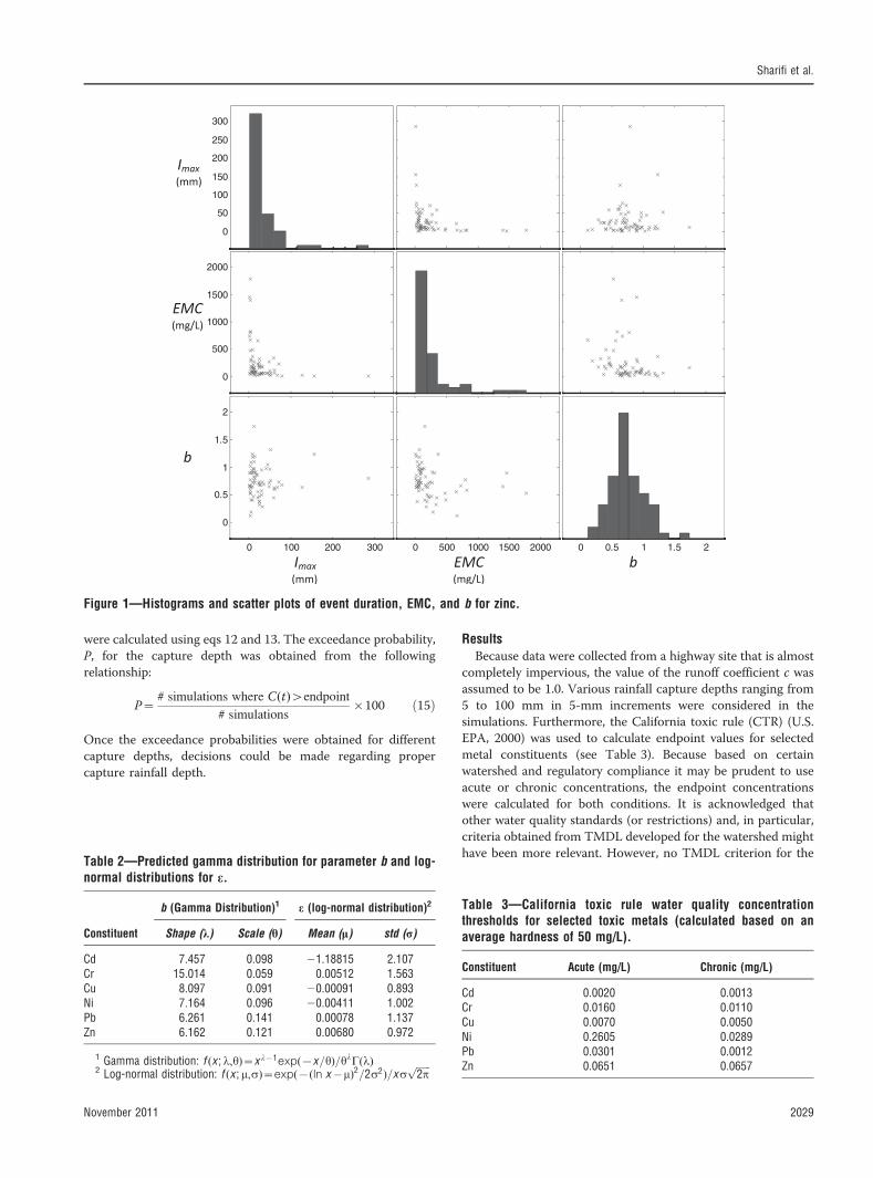
Monte Carlo Simulation. A statistical analysis was per-formed to investigate the frequency distributions and anypossible correlations among parameters b, EMC, Imax, andseveral hydrograph indicators including event duration, totalvolume, event skewness, and temporal moments of rain intensitythroughout the events. As an example, Figure 1 shows the

Sharifi et al.

November 2011 2027

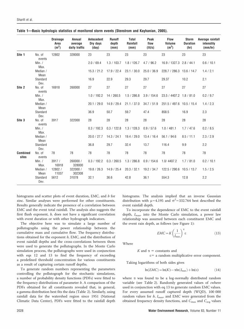
histograms and scatter plots of event duration, EMC, and b forzinc. Similar analyses were performed for other constituents.Results generally indicate the presence of a correlation betweenEMC and the event total rainfall. The analysis also suggests thefirst flush exponent, b, does not have a significant correlationwith event duration or with other hydrograph indicators.

The objective here was to simulate a large number ofpollutographs using the power relationship between thecumulative mass and cumulative flow. The frequency distribu-tions obtained for the exponent b, EMC, and the distribution ofevent rainfall depths and the cross-correlations between themwere used to generate the pollutographs. In the Monte Carlosimulation process, the pollutographs were used in conjunctionwith eqs 12 and 13 to find the frequency of exceedinga predefined threshold concentration for various constituentsas a result of capturing certain runoff depths.

To generate random numbers representing the parameterscontrolling the pollutograph for the stochastic simulations,a number of probability density functions (PDFs) were fitted tothe frequency distributions of parameter b. A comparison of thePDFs obtained for all constituents revealed that, in general,a gamma distribution best fits the data (Table 2). Similarly, usingrainfall data for the watershed region since 1951 (NationalClimatic Data Center), PDFs were fitted to the rainfall depth

histograms. The analysis implied that an inverse Gaussiandistribution with m54.195 and s25332.764 best described theevent rainfall depth.

To incorporate the dependence of EMC to the event rainfalldepth, Imax, into the Monte Carlo simulation, a power lawrelationship was assumed between each constituent EMC andthe event rain depth, as follows (see Figure 1):

EMC~K1

Imax

� �a

e ð13Þ

Where

K and a 5 constants ande5 a random multiplicative error component.

Taking logarithms of both sides gives

ln EMCð Þ~ln(K ){aln Imaxð Þzln(e) ð14Þ

where a was found to be a log-normally distributed randomvariable (see Table 2). Randomly generated values of ewhereused in conjunction with eq 13 to generate random EMC values.For every assumed runoff captured depth (WQD), 100 000random values for b, Imax, and EMC were generated from theobtained frequency density functions, and Cmax and Cavg values

Table 1—Basic hydrologic statistics of monitored storm events (Stenstrom and Kayhanian, 2005).

DrainageArea(m2)

Annualaverage

daily traffic

AntecedentDry days

(day)

Runoffdepth(mm)

TotalRainfall

(mm)

Peakflow

(lit/s)

FlowVolume

(m3)

StormDuration

(hr)

Average rainfallintenstity(mm/hr)

Site 1 No. ofevents

12802 328000 23 23 23 23 23 23 23

Min. /Max.

2.0 / 69.4 1.3 / 103.7 1.8 / 126.7 4.7 / 96.2 16.9 / 1327.3 2.8 / 44.1 0.6 / 10.1

Median /Mean

15.3 / 21.2 17.9 / 22.4 23.1 / 30.0 25.0 / 36.9 228.7 / 286.3 13.6 / 14.7 1.4 / 2.1

StandardDev.

16.9 22.9 29.3 29.7 29.37 10.2 2.1

Site 2 No. ofevents

16918 260000 27 27 27 27 27 27 27

Min. /Max.

1.0 / 192.2 14 / 260.5 1.5 / 286.8 3.9 / 154.6 23.5 / 4407.2 1.8 / 81.0 0.2 / 9.7

Median /Mean

20.1 / 29.0 14.9 / 29.4 21.1 / 37.0 34.7 / 51.9 251.5 / 497.6 10.5 / 15.4 1.4 / 2.3

StandardDev.

36.9 50.7 59.7 47.4 858.5 16.9 2.3

Site 3 No. ofevents

3917 322000 28 28 28 28 28 28 28

Min. /Max.

0.3 / 192.3 0.3 / 122.8 1.3 / 128.3 0.9 / 57.6 1.0 / 481.1 1.7 / 47.6 0.2 / 8.5

Median /Mean

20.0 / 27.7 14.3 / 24.1 19.4 / 29.0 13.4 / 16.4 56.1 / 94.6 8.5 / 11.1 2.3 / 2.9

StandardDev.

36.8 29.7 32.4 13.7 116.4 9.9 2.2

Combinedsites

No. ofevents

78 78 78 78 78 78 78 78 78

Min. /Max.

3917 /16918

260000 /328000

0.3 / 192.2 0.3 / 260.5 1.3 / 286.8 0.9 / 154.6 1.0/ 4407.2 1.7 / 81.0 0.2 / 10.1

Median /Mean

12802 /11037

322000 /302308

19.8 / 26.3 14.9 / 25.4 20.3 / 32.1 19.2 / 34.7 122.5 / 290.6 10.5 / 13.7 1.5 / 2.5

StandardDev.

5612 31078 32.1 36.6 42.8 36.1 554.3 12.8 2.2

Sharifi et al.

2028 Water Environment Research, Volume 83, Number 11

were calculated using eqs 12 and 13. The exceedance probability,P, for the capture depth was obtained from the followingrelationship:

P~# simulations where C(t)wendpoint

# simulations|100 ð15Þ

Once the exceedance probabilities were obtained for differentcapture depths, decisions could be made regarding propercapture rainfall depth.

ResultsBecause data were collected from a highway site that is almost

completely impervious, the value of the runoff coefficient c wasassumed to be 1.0. Various rainfall capture depths ranging from5 to 100 mm in 5-mm increments were considered in thesimulations. Furthermore, the California toxic rule (CTR) (U.S.EPA, 2000) was used to calculate endpoint values for selectedmetal constituents (see Table 3). Because based on certainwatershed and regulatory compliance it may be prudent to useacute or chronic concentrations, the endpoint concentrationswere calculated for both conditions. It is acknowledged thatother water quality standards (or restrictions) and, in particular,criteria obtained from TMDL developed for the watershed mighthave been more relevant. However, no TMDL criterion for the

Figure 1—Histograms and scatter plots of event duration, EMC, and b for zinc.

Table 2—Predicted gamma distribution for parameter b and log-normal distributions for e.

Constituent

b (Gamma Distribution)1 e (log-normal distribution)2

Shape (l) Scale (h) Mean (m) std (s)

Cd 7.457 0.098 21.18815 2.107Cr 15.014 0.059 0.00512 1.563Cu 8.097 0.091 20.00091 0.893Ni 7.164 0.096 20.00411 1.002Pb 6.261 0.141 0.00078 1.137Zn 6.162 0.121 0.00680 0.972

1 Gamma distribution: f (x ; l,h)~x l{1exp({x=h)=hlC(l)2 Log-normal distribution: f (x ; m,s)~exp({(ln x{m)2=2s2)=xs

ffiffiffiffiffiffi2pp

Table 3—California toxic rule water quality concentrationthresholds for selected toxic metals (calculated based on anaverage hardness of 50 mg/L).

Constituent Acute (mg/L) Chronic (mg/L)

Cd 0.0020 0.0013Cr 0.0160 0.0110Cu 0.0070 0.0050Ni 0.2605 0.0289Pb 0.0301 0.0012Zn 0.0651 0.0657

Sharifi et al.

November 2011 2029

current highway characterization study area was available at thetime of the study.

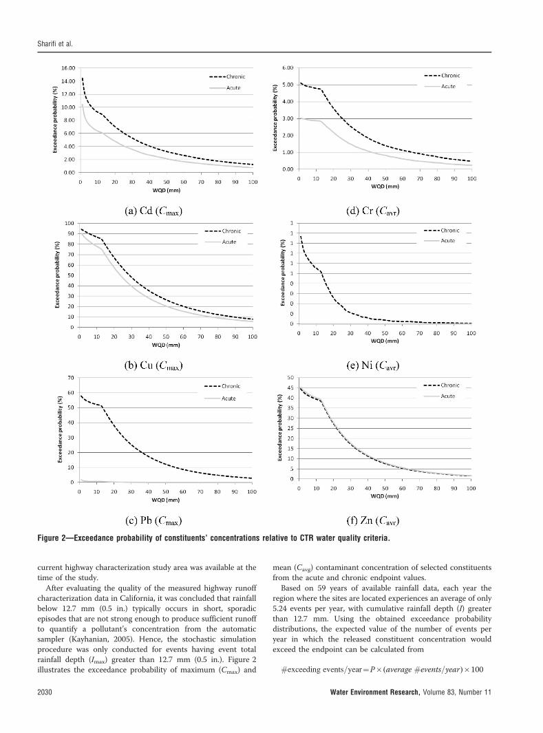
After evaluating the quality of the measured highway runoffcharacterization data in California, it was concluded that rainfallbelow 12.7 mm (0.5 in.) typically occurs in short, sporadicepisodes that are not strong enough to produce sufficient runoffto quantify a pollutant’s concentration from the automaticsampler (Kayhanian, 2005). Hence, the stochastic simulationprocedure was only conducted for events having event totalrainfall depth (Imax) greater than 12.7 mm (0.5 in.). Figure 2illustrates the exceedance probability of maximum (Cmax) and

mean (Cavg) contaminant concentration of selected constituentsfrom the acute and chronic endpoint values.

Based on 59 years of available rainfall data, each year theregion where the sites are located experiences an average of only5.24 events per year, with cumulative rainfall depth (I) greaterthan 12.7 mm. Using the obtained exceedance probabilitydistributions, the expected value of the number of events peryear in which the released constituent concentration wouldexceed the endpoint can be calculated from

#exceeding events=year~P|(average #events=year)|100

Figure 2—Exceedance probability of constituents’ concentrations relative to CTR water quality criteria.

Sharifi et al.

2030 Water Environment Research, Volume 83, Number 11

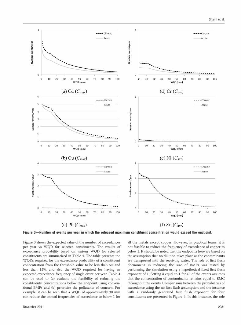
Figure 3 shows the expected value of the number of exceedancesper year vs WQD for selected constituents. The results ofexceedance probability based on various WQD for selectedconstituents are summarized in Table 4. The table presents theWQDs required for the exceedance probability of a constituentconcentration from the threshold value to be less than 5% andless than 15%, and also the WQD required for having anexpected exceedance frequency of single event per year. Table 4can be used to (a) evaluate the feasibility of reducing theconstituents’ concentrations below the endpoint using conven-tional BMPs and (b) prioritize the pollutants of concern. Forexample, it can be seen that a WQD of approximately 30 mmcan reduce the annual frequencies of exceedance to below 1 for

all the metals except copper. However, in practical terms, it isnot feasible to reduce the frequency of exceedance of copper tobelow 1. It should be noted that the endpoints here are based onthe assumption that no dilution takes place as the contaminantsare transported into the receiving water. The role of first flushphenomena in reducing the size of BMPs was tested byperforming the simulation using a hypothetical fixed first flushexponent of 1. Setting b equal to 1 for all of the events assumesthat the concentration of contaminants remains equal to EMCthroughout the events. Comparisons between the probabilities ofexceedance using the no first flush assumption and the instancewith a randomly generated first flush exponent for fourconstituents are presented in Figure 4. In this instance, the role

Figure 3—Number of events per year in which the released maximum constituent concentration would exceed the endpoint.

Sharifi et al.

November 2011 2031

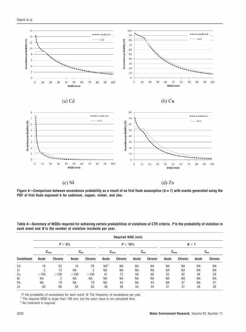
Table 4—Summary of WQDs required for achieving certain probabilities of violations of CTR criteria. P is the probability of violation ineach event and N is the number of violation incidents per year.

Constituent

Required WQD (mm)

P , 5% P , 15% N , 1

Cmax Cavr Cmax Cavr Cmax Cavr

Acute Chronic Acute Chronic Acute Chronic Acute Chronic Acute Chronic Acute Chronic

Cd 19 32 15 29 NA2 NA NA NA NA NA NA NACr 2 13 NA 2 NA NA NA NA NA NA NA NACu .100 .100 .100 .100 61 72 59 68 52 62 49 59Ni NA 2 NA NA NA NA NA NA NA NA NA NAPb NA 79 NA 79 NA 44 NA 43 NA 37 NA 37Zn 66 66 63 63 36 36 34 34 31 31 28 28

P: the probability of exceedance for each event; N: The frequency of exceedance per year.1 The required WQD is larger than 100 mm, but the exact value is not calculated here.2 No treatment is required.

Figure 4—Comparison between exceedance probability as a result of no first flush assumption (b = 1) with events generated using thePDF of first flush exponent b for cadmium, copper, nickel, and zinc.

Sharifi et al.

2032 Water Environment Research, Volume 83, Number 11

of first flush appears to not be substantial. This is because thevariability of EMCs of events dominates the concentrationvariability during each event as a result of first flush. However,this conclusion is specific to the studied site and the thresholdvalues considered and, therefore, should not be generalized.

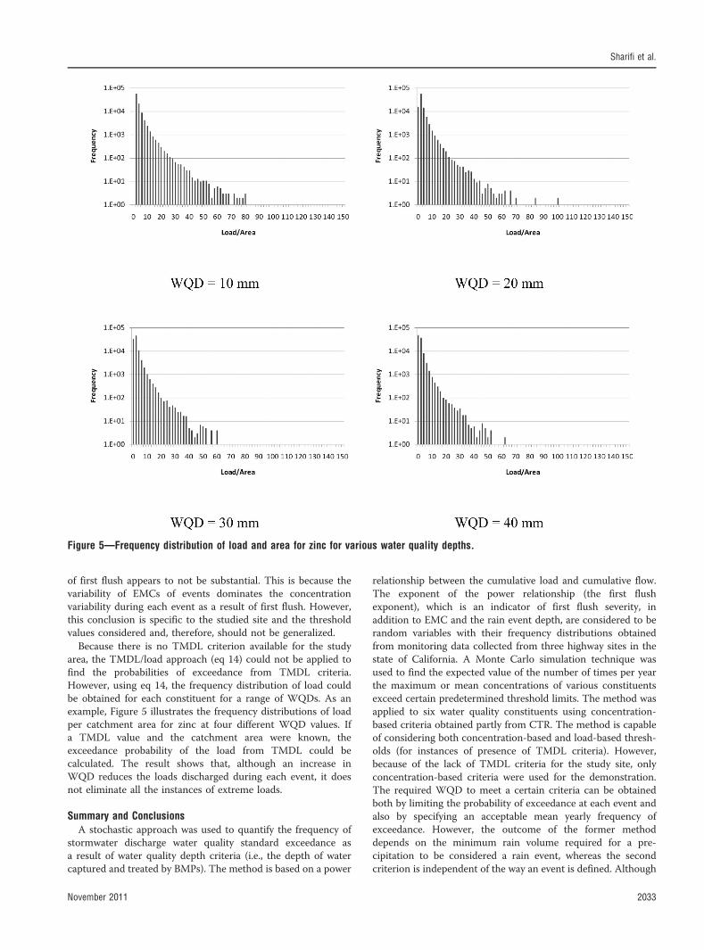
Because there is no TMDL criterion available for the studyarea, the TMDL/load approach (eq 14) could not be applied tofind the probabilities of exceedance from TMDL criteria.However, using eq 14, the frequency distribution of load couldbe obtained for each constituent for a range of WQDs. As anexample, Figure 5 illustrates the frequency distributions of loadper catchment area for zinc at four different WQD values. Ifa TMDL value and the catchment area were known, theexceedance probability of the load from TMDL could becalculated. The result shows that, although an increase inWQD reduces the loads discharged during each event, it doesnot eliminate all the instances of extreme loads.

Summary and ConclusionsA stochastic approach was used to quantify the frequency of

stormwater discharge water quality standard exceedance asa result of water quality depth criteria (i.e., the depth of watercaptured and treated by BMPs). The method is based on a power

relationship between the cumulative load and cumulative flow.The exponent of the power relationship (the first flushexponent), which is an indicator of first flush severity, inaddition to EMC and the rain event depth, are considered to berandom variables with their frequency distributions obtainedfrom monitoring data collected from three highway sites in thestate of California. A Monte Carlo simulation technique wasused to find the expected value of the number of times per yearthe maximum or mean concentrations of various constituentsexceed certain predetermined threshold limits. The method wasapplied to six water quality constituents using concentration-based criteria obtained partly from CTR. The method is capableof considering both concentration-based and load-based thresh-olds (for instances of presence of TMDL criteria). However,because of the lack of TMDL criteria for the study site, onlyconcentration-based criteria were used for the demonstration.The required WQD to meet a certain criteria can be obtainedboth by limiting the probability of exceedance at each event andalso by specifying an acceptable mean yearly frequency ofexceedance. However, the outcome of the former methoddepends on the minimum rain volume required for a pre-cipitation to be considered a rain event, whereas the secondcriterion is independent of the way an event is defined. Although

Figure 5—Frequency distribution of load and area for zinc for various water quality depths.

Sharifi et al.

November 2011 2033

the frequency of exceedance values obtained are site-specific anddepends on the water quality endpoints chosen, the approachprovides a systematic way to quantitatively evaluate the effect ofthe selection of water quality depth on the concentrations ofvarious pollutants discharged into receiving waters or to meetTMDL criteria using monitoring data. In particular, the methodoffers a simple way to prioritize pollutants during developmentof TMDL implementation plans. It also offers a means toevaluate the efficacy of forcing water quality depth criteria forsatisfying TMDL or concentration criteria in complicated urbansettings where the use of distributed or lumped parameterwatershed water quality models is difficult and involves largeuncertainties. It should be noted that the method proposed hereassumes that the watershed size is small enough so that its timeof concentration is small relative to the rain-intensity fluctuationtime scale. This assumption should be used with caution forlarge watersheds. Moreover, the applicability of the powerrelationship for approximating the normalized cumulative loadvs flow curves needs to be verified with pollutograph datacollected from a larger number of sites. In addition, in the modelapplication presented here, it was assumed that the runoffcoefficient c is independent of rain intensity. In applications tolarge watersheds, such dependencies can be incorporated byexplicitly expressing c as a function of rain intensity in theMonte Carlo simulation.

The main conclusions drawn from this study are as follows:

N A half-inch WQD seems to reduce the frequency ofexceeding the concentration-based criteria significantly formost constituents. However, in some instances, even muchlarger WQDs will not satisfy concentration-based criteria.

N The BMP design criteria based on a required water qualitydepth seems to be more effective in reducing the probabilityof exceeding load-based criteria than a concentration-basedcriteria.

N For the data set used in this study, it was found that the roleof event first flush on the effect of water quality depth onexceedance frequencies is not significant. This is becausethe exceedance probability is dominated mostly by thelarger variability in EMCs of events. Therefore, consideringfirst flush will not result in substantially smaller waterquality depth criteria.

NotationsA 5 drainage areab 5 first flush exponent M(t)~½V (t)�bC 5 constituent concentrationc 5 runoff coefficientI 5 cumulative rainfall depthi 5 rainfall intensity

K 5 constant in eq 13M 5 dimensionless cumulative constituent massP 5 exceedance probabilityT 5 duration of the entire eventt 5 time

V 5 dimensionless cumulative flowa 5 constant in eq 13C 5 gamma functione 5 random error componenth 5 scale factor in Gamma function

l 5 shape factor in Gamma functions2 5 variancem 5 average

Subscriptsavg 5 average value

max 5 maximum value (at the end of rainfall)

AcronymsEMC 5 event mean concentration

FF 5 first flushPDF 5 probability density function

TMDL 5 total daily maximum loadWQD 5 water quality depthWQV 5 water quality volume

Credits

Data used in this study were obtained from first flush highwayrunoff characterization that was funded by the Division ofEnvironmental Analysis, California Department of Transportation.The first flush characterization study was performed undercollaborative efforts between the Departments of Civil andEnvironmental Engineering at the University of California at LosAngeles and the University of California at Davis. The authors areespecially thankful to Professor Mike Stenstrom and his graduatestudents and research staff for all of their efforts and contributionsduring the study period. Partial funding for this study was providedby the District of Columbia Water Resources Research Institute.

Submitted for publication August 26, 2010; revised manuscriptsubmitted January 31, 2011; accepted for publication March 14,2011.

ReferencesAhlfeld, D. P.; Minihane, M. (2004) Storm Flow from First-Flush

Precipitation in Stormwater Design. J. Irrigation Drainage Eng., 130(4), 269.

Balades, J. D.; Legret, M.; Madiec, H. (1995) Permeable Pavements—Pollution Management Tools. Water Sci. Technol., 32 (1), 49.

Barco, J.; Papiri, S.; Stenstrom, M. K. (2008) First Flush in a CombinedSewer System. Chemosphere, 71 (5), 827.

Barrett, M. E.; Irish, L. B.; Malina, J. F.; Charbeneau, R. J. (1998)Characterization of Highway Runoff in Austin, Texas, Area. J.Environ. Eng., 124 (2), 131.

Bertrand-Krajewski, J. L.; Chebbo, G.; Saget, A. (1998) Distribution ofPollutant Mass Vs Volume in Stormwater Discharges and the FirstFlush Phenomenon. Water Res., 32 (8), 2341.

Chang, G.; Parrish, J.; Souer, C. (1990) The First Flush of Runoff and ItsEffect on Control Structure Design. Final Report; Environmentaland Conservation Services Department, Environmental ResourcesManagement Division: Austin, Texas.

Charbeneau, R. J.; Barrett, M. E. (1998) Evaluation of Methods forEstimating Stormwater Pollutant Loads. Water Environ. Res., 70 (7),1295.

Cristina, C. M.; Sansalone, J. J. (2003) ‘‘First Flush,’’ Power Law andParticle Separation Diagrams for Urban Stormwater SuspendedParticulates. J. Environ. Eng., 129 (4), 298.

Davis, A. P. (2008) Field Performance of Bioretention: HydrologyImpacts. J. Hydrologic Eng., 13 (2), 90.

Deletic, A. (1998) The First Flush Load of Urban Surface Runoff. WaterRes., 32 (8), 2462.

Deletic, A. B.; Maksimovic, C. T. (1998) Evaluation of Water QualityFactors in Storm Runoff from Paved Areas. J. Environ. Eng., 124 (9),869.

Sharifi et al.

2034 Water Environment Research, Volume 83, Number 11

Deng, Z. Q.; de Lima, J.; Singh, V. P. (2005) Fractional Kinetic Model forFirst Flush of Stormwater Pollutants. J. Environ. Eng., 131 (2), 232.

Ellis, J. B. (1986) Probabilistic Modelling of Urban Runoff Quality. InWater Quality Modelling in the Inland Natural Environment;British Hydrodynamics Research Association: Cranfield, Bedford-shire, U.K.; pp 551–558.

England, G. (2001) The Use of Ponds as BMPs. Stormwater, 2 (5), 40.Flint, K. R.; Davis, A. P. (2007) Pollutant Mass Flushing Characterization

of Highway Stormwater Runoff from an Ultra-Urban Area. J.Environ. Eng., 133 (6), 616.

Froehlich, D. C. (2009) Graphical Calculation of First-Flush Flow Ratesfor Storm-Water Quality Control. J. Irrigation Drainage Eng., 135(1), 68.

Geiger, W. (1987) Flushing Effects in Combined Sewer Systems.Proceedings of the 4th International Conference on Urban Drainage;Lausanne, Switzerland; pp 40–46.

Gupta, K.; Saul, A. J. (1996) Specific Relationship for the First Flush Loadin Combined Sewer Flows. Water Res., 30 (5), 1244.

Han, Y. H.; Lau, S. L.; Kayhanian, M.; Stenstrom, M. K. (2006)Correlation Analysis among Highway Stormwater Pollutants andCharacteristics. Water Sci. Technol., 53 (2), 235.

Horan, N. J. (1990) Biological Wastewater Treatment Systems: Theoryand Operation; Wiley & Sons: London, United Kingdom.

Hsieh, C. H.; Davis, A. P. (2005) Multiple-Event Study of Bioretention forTreatment of Urban Storm Water Runoff. Water Sci. Technol., 51(3–4), 177.

Huber, W. C. (1993) Contaminant Transport in Surface Water. InHandbook of Hydrology; Maidment, D. R., Ed.; McGraw-Hill: NewYork; pp 14.11–14.50.

Jefferies, C.; Aitken, A.; McLean, N.; Macdonald, K.; McKissock, G.(1999) Assessing the Performance of Urban BMPs in Scotland.Water Sci. Technol., 39 (12), 123.

Kang, J. H.; Kayhanian, M.; Stenstrom, M. K. (2006) Implications ofa Kinematic Wave Model for First Flush Treatment Design. WaterRes., 40 (20), 3820.

Kang, J. H.; Kayhanian, M.; Stenstrom, M. K. (2008) Predicting theExisting of Stormwater First Flush from the Time of Concentration.Water Res., 42 (1–2), 220.

Kayhanian, M. (2005) Advanced Stormwater Runoff Characterization.Proceedings of the 10th International Conference on UrbanDrainage; Copenhagen, Denmark; Aug 21–26.

Kayhanian M.; Stenstrom, M. K. (2005) First Flush Pollutant MassLoading: Treatment Strategies. In Transportation Research Record(Hydrology, Hydraulics, and Water Quality); No. 1904; pp 133–143.

Kim, L. H.; Kayhanian, M.; Zoh, K. D.; Stenstrom, M. K. (2005) Modelingof Highway Stormwater Runoff. Sci. Total Environ., 348 (1–3), 1.

Larsen, T.; Broch, K.; Andersen, M. R. (1998) First Flush Effects in anUrban Catchment Area in Aalborg. Water Sci. Technol., 37 (1), 251.

Lee, H.; Lau, S. L.; Kayhanian, M.; Stenstrom, M. K. (2004) Seasonal FirstFlush Phenomenon of Urban Stormwater Discharges. Water Res.,38 (19), 4153.

Martinson, D. B.; Thomas, T. (2005) Low-Cost Inlet Filters for RainwaterTanks. Proceedings of the 12th International Rainwater CatchmentSystems Conference; New Delhi, India.

Massachusetts Department of Environmental Protection (1997) Storm-water Management, Volume One: Stormwater Policy Handbook;State of Massachusetts Publication No. 17871-250-1800-4/97-6.52-C.R.; Massachusetts Department of Environmental Protection:Boston, Massachusetts.

Massoudieh, A.; Abrishamchi, A.; Kayhanian, M. (2008) MathematicalModeling of First Flush in Highway Storm Runoff using GeneticAlgorithm. Sci. Total Environ., 398 (1–3), 107.

Minnesota Pollution Control Agency (2008) Minnesota StormwaterManual. http://www.pca.state.mn.us/publications/wq-strm9-01.pdf.http://www.pca.state.mn.us/index.php/view-document.html?gid5

8937 (accessed July 28, 2011).National Climatic Data Center. Water Year Data, 1950–2010, Los

Angeles Airport Station. http://www4.ncdc.noaa.gov/cgi-win/wwcgi.dll?wwDIStnSrchStnID20001642#DAF (accessed Aug 16,2010).

New Hampshire Department of Environmental Services (2008) NewHampshire Stormwater Manual; Volume 2, Post-Construction BestManagement Practices Selection & Design. http://des.nh.gov/organization/commissioner/pip/publications/wd/documents/wd-08-20b.pdf (accessed July 28, 2011).

Rhode Island Department of Environmental Management; CoastalResources Management Council (2010) Rhode Island StormwaterDesign and Installation Standards Manual. http://www.dem.ri.gov/pubs/regs/regs/water/swmanual.pdf (accessed July 28, 2011).

Saget, A.; Chebbo, G.; Bertrand-Krajewski, J. L. (1996) The First Flush inSewer Systems. Water Sci. Technol., 33 (9), 101.

Sartor, J. D.; Boyd, G. B. (1972) Water Pollution Aspects of Street SurfaceContaminants; EPA-R2/72-081; U.S. Environmental ProtectionAgency: Washington, D.C.

Sansalone, J. J.; Buchberger, S. G. (1997) Partitioning and First Flush ofMetals in Urban Roadway Storm Water. J. Environ. Eng., 123 (2),134.

Sansalone, J. J.; Cristina, C. M. (2004) First Flush Concepts for Suspendedand Dissolved Solids in Small Impervious Watersheds. J. Environ.Eng., 130 (11), 1301.

Stahre, P.; Urbonas, B. (1990) Storm-Water Detention for Drainage,Water Quality and CSO Management; Prentice Hall: EngelwoodCliffs, New Jersey.

Stenstrom, M. K.; Kayhanian, M. (2005) First Flush PhenomenonCharacterization; California Department of Transportation, Di-vision of Environmental Analysis: Sacramento, California.

U.S. Environmental Protection Agency (2000) Water QualityStandards; Establishment of Numeric Criteria for Priority ToxicPollutants for the State of California; Rule. Fed. Regist., 65 (97),31682.

U.S. Environmental Protection Agency (2004) Stormwater Best Man-agement Design Guide: Volume 1, General Considerations; EPA-600/R-04-121; U.S. Environmental Protection Agency, Office ofResearch and Development: Washington, D.C.

Wanielista, M. P.; Yousef, Y. A.; McLellon, W. M. (1977) NonpointSource Effects on Water Quality. J.— Water Pollut. Control Fed., 49(3), 441.

Sharifi et al.

November 2011 2035