A Statistical comparative analysis of Simulated … · A Statistical comparative analysis of Simulated Annealing and Variable Neighborhood Search … 297 Computación y Sistemas Vol

Computación y Sistemas Vol. 14 No. 3, 2011 pp 295-308 ISSN 1405-5546

A Statistical comparative analysis of Simulated Annealing and Variable Neighborhood Search for the Geographic Clustering

Problem

Un Análisis Estadístico Comparativo de Recocido Simulado y Búsqueda de Vecindad Variable para el Problema de Agregación Geográfica

Beatriz Bernábe Loranca1, José E. Espinosa Rosales2, Javier Ramírez Rodriguez3 and María A. Osorio Lama4

1Facultad de Ciencias de la Computación, Benemérita Universidad Autónoma de Puebla Puebla, México

[email protected] 2Facultad de Ciencias Físico Matemáticas, Benemérita Universidad Autónoma de Puebla

Puebla, México [email protected]

3Departamento de Sistemas, Universidad Autónoma Metropolitana Distrito Federal, México

[email protected] 4Facultad de Ingeniería Química, Benemérita Universidad Autónoma de Puebla

Puebla, México [email protected]

Article received on October 23, 2009; accepted on May 06, 2010

Abstract. This paper describes a factorial statistical study that compares the quality of solutions produced by two heuristics: Simulated Annealing (SA) and Variable Neighborhood Search (VNS). These methods are used to solve the Geographic Clustering Problem (GCP), and the quality of the solutions produced for specific times has been compared. With the goal of comparing the quality of the solutions, where both heuristics participate in an impartial evaluation, time has been the only common element considered for VNS and SA. At this point, two factorial experiments were designed and the corresponding parameters for each heuristic were carefully modeled leaving time as the cost function. In instances of 24 objects, the experiments involved the execution of two sets of tests recording the results of the different response times and the associated values of the objective function for each heuristic and instance conditions. The solution to this problem requires a partitioning process where each group is composed of objects that fulfill better the objective: the minimum accumulated distance from the objects to the centroid of each group. The GCP is a combinatorial NP-hard problem (Bação, Lobo and Painho, 2004). Keywords: Algorithms, Design, Experimentation, Geographic Clustering Problem, Heuristics. Resumen. Este artículo describe un estudio estadístico factorial para comparar la calidad de las soluciones de dos heurísticas: Recocido Simulado (RS) y Búsqueda en Entorno Variable (BEV). Estos métodos son usados para resolver el

problema de agregación geográfica, y se han comparado de acuerdo a la calidad de las soluciones obtenidas en tiempos específicos estimados. Con el objetivo de comparar la calidad de las soluciones, donde las dos heurísticas participen en una evaluación equitativa, se ha considerado el tiempo como el único elemento común para BEV y RS. En este punto, se diseñaron dos experimentos factoriales donde se modelaron cuidadosamente los parámetros correspondientes para cada heurística dejando como función de costo al tiempo. Estos experimentos implicaron la ejecución de dos conjuntos de pruebas para instancias de 24 objetos registrándose los resultados de los diferentes tiempos de respuesta y los valores asociados de la función objetivo para cada heurística. La solución a este problema requiere un proceso de particionamiento donde cada grupo está formado de objetos que cumplen mejor con el objetivo: la distancia mínima acumulada de los objetos al centroide en cada grupo. El problema de agregación geográfica es combinatorio NP-duro (Bação, Lobo and Painho, 2004). Palabras clave: Algoritmos, Diseño, Experimentación, Problema de Agrupamiento Geográfico, Heurísticas.

1 Introduction

The GCP consists in the classification of objects in geographic units that meet certain objectives, mainly the geometric compactness (Bação, Lobo and

296 Beatriz Bernábe Loranca, José E. Espinosa Rosales, Javier Ramírez Rodríguez and María A. Osorio Lama


Painho, 2004). The geographic units that have been considered correspond to AGEBs (Basic Geo-Statistical Areas) from the metropolitan zone of the Toluca Valley (MZTV) (INEGI, 2000).

The GCP problem belongs to the Territorial Design (TD) category and it is understood as the problem of grouping small geographic areas (basic areas) in larger geographical clusters called territories, in such a way that the acceptable grouping is one that meets certain predetermined criteria (Zoltners and Sinha, 1983). The criteria or properties to meet in GCP problems depend on the constraint space and the geometric compactness (Murtagh, 1991). The NP-hard condition of the GCP implies having to solve a large number of geographic tasks that emphasizes the classification process directed towards meeting an objective.

Therefore, this problem is usually explained with a description in terms of an optimization objective modeled mathematically as a cost function complemented by the characteristics of the problem expressed as constraints. The NP-hard nature of this problem justifies the use of heuristics to obtain good solutions in a reasonable amount of time. The GCP is a special case of the classic clustering problem, but with the requirement of compactness, connectedness and/or homogeneity in some cases (Murtagh, 1991; Zoltners and Sinha, 1983).

To solve the GCP, we developed our own partitioning algorithm that minimizes the distances between the objects, in order to obtain compactness between the AGEBs (Bernábe, 2009 and 2009a). However, the primary goal of this research goes beyond presenting the solutions generated by VNS (Hansen and Mladenovic, 1996 and 2003) and SA (Kirkpatrick, Gelatt and Vecchi, 1983).

Our main contribution is centered exactly in this point: we used the optimal solutions obtained with SA (Bernábe, 2009) and compared them with the solutions generated with VNS for the GCP (Bernábe, 2009a) using a Box Behnken experimental design (Montgomery, 1991) with different selected times, to evaluate the quality of the solutions.

This paper is organized as follows. In section 2 we present the mathematical model for the GCP. Section 3 describes the solution to the GCP with SA and with VNS. Section 4 describes the results obtained for the Box Behnken design with VNS and section 5 presents the Box Behnken design with SA. Finally some conclusions are presented in section 6.

2.Mathematical model for the Geographic Clustering Problem (GCP)

Many approaches have been used to solve the GCP. The method utilized in this research to solve the AGEBs conglomerate design is similar to the method presented in (Bação, Lobo and Painho, 2004), where the authors implemented a genetic algorithm for a similar zone design problem. In the GCP solved here, the AGEBs are geographical units where each AGEB is separated by different distances of non uniform geometric structure, because the AGEBs are spatial data and its geographical localization is given by latitude and longitude, it was easier to calculate the distances between them (Zamora, 2006). The AGEBs are clustered in territories (groups) that are very close geographically, in order to minimize the distances between them. Basically, the strategy is to randomly choose AGEBs as centroids to identify the territory (group). Those AGEBs that are not centroids and have the shortest distance to a specific centroid-AGEB are members of the same territory or cluster. This informal idea is the definition of geometrical compactness. The definition of compactness for geographic units is included in Definition 1: Definition 1. Let n,..,,Z 21 be the set of n objects

to cluster; the objective is to divide Z in k groups ZG..,GG k,, 21 with nk , such that:

ZGk1i i

ji GG , ji

1iG ki ,..,1

A group mG with 1mG is compact if every object

Gmt satisfies:

mm G-Zj tiGi

jt,d Min itd Min

,

)(),(

A group mG with 1mG is compact only if its

object t satisfies:

m f Gflj, tZi

lt,d Min itd Min

)(),(

(1)

A Statistical comparative analysis of Simulated Annealing and Variable Neighborhood Search … 297

Computación y Sistemas Vol. 14 No. 3, 2011 pp 295-308

ISSN 1405-5546

The neighborhood criterion between objects, needed to achieve the compactness, is given by the pairs of distances described in (1). Using this definition of compactness we will proceed to describe the model for the GCP. Effectively, it is possible to rewrite definition 1 and extend it to a general optimization model for geographical partitioning, in this way the data, restrictions and objective function are identified. So it is understood that the GCP model may have different algorithmic translation (pseudo code) and/or implementations when a heuristic method is introduced (Bernábe, 2009 and 2009a). In this work the model had two extensions with variants in the implementation owing to, among other things, the difference in obtaining neighboring solutions for each heuristic: a) Model for GCP with SA and b) Model for GCP with VNS. A model with different capacity can be built with the inclusion of another heuristic method, and hybrid between RS and VNS for example; this is a work in progress. There is a detailed explanation with pseudo code in section 3 about how SA and VNS obtain their respective neighboring solutions for this problem.

2.1 Model GCP

The following describes the model for GCP. Data

gU total of AGEBs Let the initial set of n geographical units be

n,...,,g xxxU 21 where

ix is the thi geographical unit ( gUi index)

k is the number of the zone (group). The following variables are defined to refer to the different groups:

iZ is the set of geographical units that belong to the

thi zone n is the number of geographical units

tC is the centroid

j)d(i, is the Euclidean distance from node i to node j

(from one AGEB to another) Constraints

iZ for ki ,..,1 (nonempty groups)

ji ZZ for ji (the same AGEBs cannot be

in different groups)

gki i UZ 1 (The union of all the groups are all

the AGEBs). Objective Function Once the number of centroids (k) is decided ( tC with

ki ,..,1 ), the centroids will be randomly selected and the AGEBs will be assigned to the nearest centroids. Then, for each AGEBi, the objective function is defined as the minimum of the sum of the distances between the centroids (for each k), and the AGEBs assigned to them (each AGEB is assigned to the closest centroid). For every k (where n,..,k 1 ) the sum of the distances from every AGEBs assigned to each centroid is calculated, and the minimum is selected. Therefore the objective function can be written as:

k

t i t

n,...,k tit c )ci, (dMin

11}{ (2)

where nit is the number of iterations.

3.Variable Neighborhood Search (VNS) and Simulated Annealing (SA) in the Geographical Clustering Problem

In this section the VNS and SA are introduced, as they are commonly discussed in the literature, and also the algorithmic adaptation of each heuristic to the geographical clustering model.

3.1 The Variable Neighborhood Search (VNS)

The VNS metaheuristic, proposed by Hansen and Mladenovic (1996 and 2003) is based on the observation that local minima tend to cluster in one or more areas of the searching space. Therefore when a local optimum is found, one can get advantage of the information it contains. For example, the value of several variables may be equal or close to their values at the global optimum. Looking for better solutions, VNS starts exploring, first the nearby neighborhoods of its current solution, and gradually the more distant ones. There is a current solution Sa and a neighborhood of order k associated to each iteration of VNS. Two steps are executed in every iteration: first, the generation of a neighbor solution of Sa, named Sp Nk(Sa), and second, the application of a local search



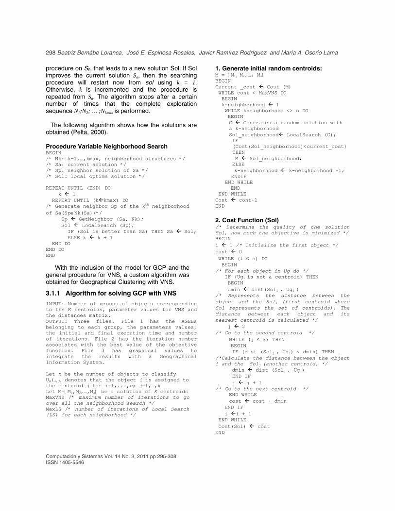
procedure on Sp, that leads to a new solution Sol. If Sol improves the current solution Sa, then the searching procedure will restart now from sol using k = 1. Otherwise, k is incremented and the procedure is repeated from Sa. The algorithm stops after a certain number of times that the complete exploration sequence N1;N2; … ;Nkmax is performed. The following algorithm shows how the solutions are obtained (Pelta, 2000). Procedure Variable Neighborhood Search BEGIN /* Nk: k=1,…,kmax, neighborhood structures */ /* Sa: current solution */ /* Sp: neighbor solution of Sa */ /* Sol: local optima solution */ REPEAT UNTIL (END) DO k 1 REPEAT UNTIL (kkmax) DO /* Generate neighbor Sp of the kth neighborhood of Sa(SpNk(Sa))*/ Sp GetNeighbor (Sa, Nk); Sol LocalSearch (Sp); IF (Sol is better than Sa) THEN Sa Sol; ELSE k k + 1 END DO END DO END With the inclusion of the model for GCP and the general procedure for VNS, a custom algorithm was obtained for Geographical Clustering with VNS.

3.1.1 Algorithm for solving GCP with VNS

INPUT: Number of groups of objects corresponding to the K centroids, parameter values for VNS and the distances matrix. OUTPUT: Three files. File 1 has the AGEBs belonging to each group, the parameters values, the initial and final execution time and number of iterations. File 2 has the iteration number associated with the best value of the objective function. File 3 has graphical values to integrate the results with a Geographical Information System. Let n be the number of objects to classify Ug(i,j) denotes that the object i is assigned to the centroid j for i=1,...,n; j=1,…,k Let M={M1,M2,…,Mk} be a solution of K centroids MaxVNS /* maximum number of iterations to go over all the neighborhood search */ MaxLS /* number of iterations of Local Search (LS) for each neighborhood */

1. Generate initial random centroids: M = {M1, M2,…, Mk} BEGIN Current _cost Cost (M) WHILE cont < MaxVNS DO BEGIN k-neighborhood 1

WHILE kneighborhood <> n DO BEGIN

C Generates a random solution with a k-neighborhood

Sol_neighborhood LocalSearch (C); IF

(Cost(Sol_neighborhood)<current_cost) THEN

M Sol_neighborhood; ELSE k-neighborhood k-neighborhood +1; ENDIF END WHILE

END END WHILE Cont cont+1 END 2. Cost Function (Sol) /* Determine the quality of the solution Sol, how much the objective is minimized */ BEGIN i 1 /* Initialize the first object */ cost 0 WHILE (i n) DO BEGIN /* For each object in Ug do */ IF (Ugi is not a centroid) THEN BEGIN dmin dist(Sol1 , Ugi ) /* Represents the distance between the object and the Sol1 (first centroid where Sol represents the set of centroids). The distance between each object and its nearest centroid is calculated */ j 2 /* Go to the second centroid */ WHILE (j k) THEN BEGIN IF (dist (Solj , Ugi) < dmin) THEN /*Calculate the distance between the object i and the Solj (another centroid) */ dmin dist (Solj , Ugi) END IF j j + 1 /* Go to the next centroid */ END WHILE cost cost + dmin END IF i i + 1 END WHILE Cost(Sol) cost END



ISSN 1405-5546

Remarks about VNS in GCP The former pseudo code describes how neighbor solutions are obtained, moreover, it is observed that an initial solution is of the form (c1, c2, ..., ck) where K specifies the number of territories (groups) and the centroids are chosen at random.

If a neighbor solution in geographical clustering means to change a centroid ci for another ci’ then it is necessary to determine which centroids are changed and which remain fixed to ensure the creation of a neighbor solution. For example, when c1, the first element of the solution, is kept fixed, a neighborhood is created by varying the last component ck with ck’. Evidently, if the initial solution is (c1, c2, ..., ck) then (c1, c2, ..., ck’) can be considered a neighbor solution. The criterion to establish the method for changing the centroid that is not fixed consists in randomly choosing another centroid ci’ to replace centroid ci using a distance threshold between ci and ci’ within a given interval.

However, changing the centroid of one territory will necessarily generate a change in at least one of the other territories since a rearrangement of its members is invariably generated.

The objective function is calculated between the centroids and the objects of its respective clusters, if there is an improvement in the solution, it is taken into account, otherwise another centroid is chosen until the stopping criterion is met (like the VNS criteria).

When a solution is generated within a neighborhood, it is supplied to the local search procedure in order to find a local optimum (that improves the solution) or until the maximum number of iterations is reached. When the solution of the local search procedure is returned (either improved or not), it is evaluated in order to decide whether a solution of the same neighborhood is generated (if there is an improvement) or a new neighborhood is selected (if there is no improvement over the current solution). Clarifying, the expression “centroid” in the algorithms described here does not mean the object at the center of the groups, in this case it could be at any coordinate within the group (territory).

The general VNS procedure does not state that the number of neighborhoods must be equal to the number of objects, but this rule was adopted during the algorithmic and implementation phases due to its usefulness for the problem being solved.

Finally, the Local Search (LS) algorithm improves the search of the current solution in its neighborhood. It can end up finding a better solution

or reaching the maximum number of iterations. The maximum number of iterations avoids the algorithm cycling in the case that a better solution cannot be found.

3.2 The Simulated Annealing (SA)

The SA algorithm is a neighborhood-based search method characterized by an acceptance criterion for neighboring solutions that adapts itself at run time. It uses a parameter called temperature (T), that according to its value determines the degree in which worse neighboring solutions can be accepted. The temperature variable is initialized with a high value, called initial temperature T0 and is reduced with each iteration through a cooling temperature mechanism (cooling factor α) until a final temperature (Tf) is reached. During each iteration a concrete number of neighbors L(T) is generated, which may be fixed for all the execution time or may change for each iteration. Each time a neighbor is generated, an acceptance criterion is applied to determine if it will substitute the current solution (Kirkpatrick, Gelatt and Vecchi, 1983).

If the neighbor solution is better than the current one, it is automatically accepted, as a classic local search would do (LS). On the contrary, if it is worse, there still exists the possibility for the neighbor to substitute the current solution. This allows the algorithm to escape from local optima, where LS would get trapped. The higher the temperature, the more likely it is to accept worse solutions. In this way, the algorithm accepts solutions much worse than the current one at the beginning of the execution (exploring) but not at the end (exploiting).

At the stage of transition between solutions a new neighbor solution (candidate) is generated by randomly disturbing any centroid (replacing it with another object), and the cost difference between the current solution and the neighbor is calculated. A smaller cost difference increases the probability of accepting worse solutions. Every time a neighbor is generated the acceptance criterion is applied to determine whether it replaces the current solution.

The cost difference in this problem depends on the objective function, which is formulated to minimize distances from the objects to the centroids. Furthermore, L(T) must be “big enough”, in this case of geographical clustering it is fixed in such a way as to reaching a stationary state for that temperature. The general procedure for simulated annealing is



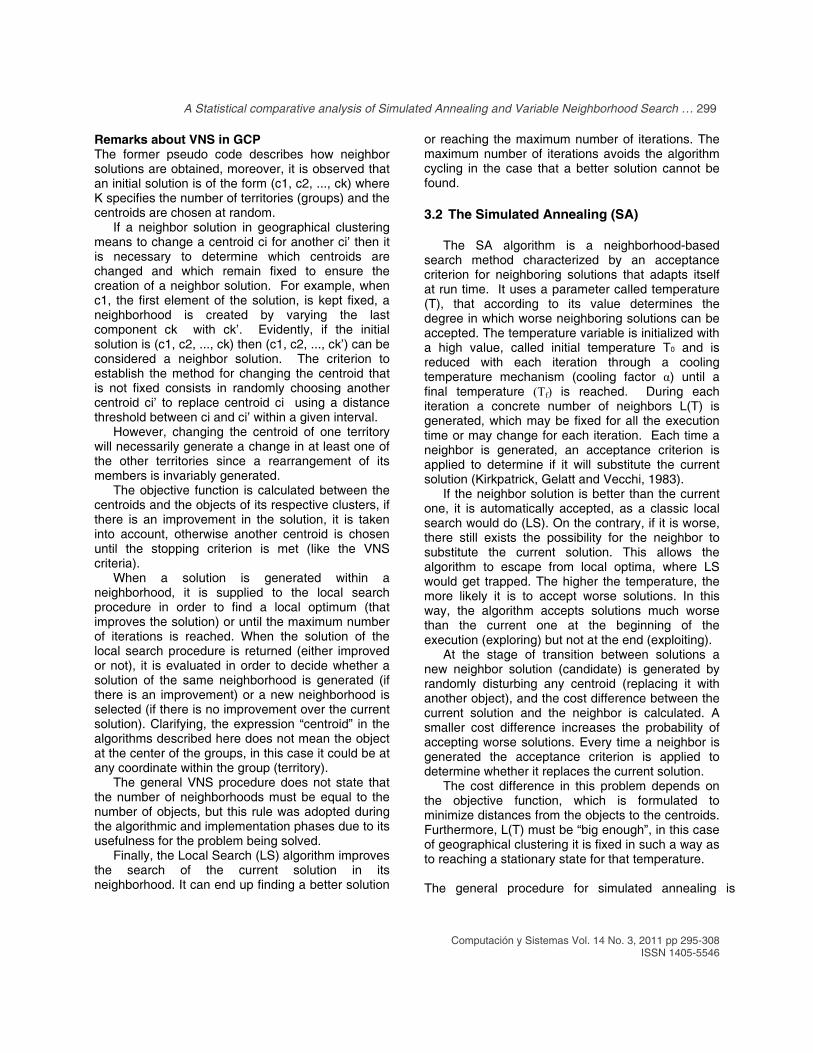
presented as follows (Dowsland, 2003): Procedure Simulated Annealing (SA) INPUT (To, α, L(t), Tf) T To /* Initial value for the control parameter* / Scur Generate initial solution WHILE T Tf DO /* Stopping condition */ BEGIN FOR cont 1 TO L(T) DO /* Cooling speed(T) */ BEGIN Scand Select solution N(Scur) /* Creation of a new solution */ cost(Scand) - cost(Scur) /* Computation of cost difference */ IF (U(0,1) < e(-/T) OR <0) THEN Scur Scand /* Acceptance criterion*/ END Tα*T /* Cooling mechanism */ END {/* WRITE as solution the best of the visited Scur*/}

By incorporating this procedure (Dowsland, 2003) to the geographical clustering model, an appropriate algorithm for geographical clustering with simulated annealing is obtained.

3.2.1 Algorithm for solving GCP with VNS

Simulated annealing and partitioning algorithm for the geographical clustering problem.

INPUT: Number of groups of objects corresponding to the K centroids, Parameter values for SA and the distances matrix.

OUTPUT: Three files. File 1 has the AGEBs belonging to each group, the parameters values, the initial and final execution time and number of iterations. File 2 has the iteration number associated with the best value of the objective function. File 3 has graphical values to integrate the results with a Geographical Information System.

Let n be the number of objects to classify Ug(i,j) denotes object i is assigned to centroid j for i = 1, …, n and j = 1, …, k Let M={M1, M2, …, Mk} be a solution with k centroids Let T0 be the initial temperature Let Tf be the final temperature Let L(t) be the number of iterations to be performed with temperature t

1..Randomly generate the initial solution M = {M1, M2, …, Mk} /* Obtain the initial solution. Any AGEB can be a randomly chosen centroid */ BEGIN Current_cost <- Cost(M)@ /* This assignment already represents an initial solution or it is a proposed solution generated by the previous iteration. The following steps generate another solution (neighbor solution) to determine how good it is compared to the current one and decide whether it is replaced or not */ WHILE T>=Tf /* While the system has not cooled down */ FOR count=1 to L(t) DO /* Number of iterations to perform with the same temperature (Parameter of SA) */ C <- Random solution /* A solution to be compared to @ is generated */ Cost_cand <- Cost(C) /* The cost of the candidate solution just generated is obtained */ <- Cost_cand – Current_cost /* Cost difference to obtain the probability of accepting the candidate solution */ IF U(0,1) < e-/T or <0 THEN /* If the acceptance probability is still high */ M <-C /* The candidate solution is accepted */ Current_cost <- Cost_cand END IF END FOR t <- *t /* The system is cooling down */ END WHILE END 2. Function Cost(Sol) /* Determines how good the solution Sol */ i <- 1 /* Initializes the first object */ Cost <- 0 WHILE i<= n /* for each object in Ug do */ IF Ugi is not a centroid THEN dmin <- dist(Sol1, Ugi) /*represents the distance from the object Ugi to Sol1 (first centroid, where Sol represents the set of all centroids). The distance from each object to the nearest centroid is calculated (distance from the object Ugi, which is not centroid to Sol1, which is centroid*/ j <- 2 /* proceeds to the second centroid */ WHILE j<= k THEN IF dist(Soli, Ugi) < dmin /* The distance from the object Ugi to Solj (another centroid) is calculated */ dmin <- dist(Solj, Ugi) END IF i <- i+1 END WHILE Cost(Sol) <- cost



ISSN 1405-5546

4 Statistical Analysis

With the purpose of developing systematic experiments to evaluate the locality of the solutions from the heuristics discussed here, several experimental schemes can be proposed, such as factorial designs, fractional factorial designs, Box Behnken designs or central composite designs (Montgomery, 1991). A matrix D(n×k) represents some of these schemes, where n is the number of combinations (treatments) for the values of the k factors (input variables for the process, parameters in this case) and there are r possible answers for each of the n combinations; with the information produced by the experiment, it is possible to individually model each of the r answers. As a general rule this models are linear or quadratic and are a function of the k factors. To develop a comparative statistical analysis about the quality of the solutions as a function of time between VNS and SA, the Box Behnken factorial was employed. The characteristics of this type of design make it easy to carry out experiments, defining adapted levels of the design parameters. Furthermore, it is a rotary design that uses equal variance for all the experimentation points that have the same distance to the center of the design, and it is possible to make sequential experiments in the pruned regions, in order to study the individual effects of the control parameters and its combined effects (Montgomery, 1991). The experimental process in this work was performed in stages. The first allowed determining the values of the parameters that improved the quality of the solutions independently of time. The second stage takes the levels that influence the experiment in the first stage; the most important values were analyzed in parallel and thus it was possible to perform new random tests around these parameters; lastly, an experimental design area was detected. These results contributed to modeling an experiment where the heuristics parameters were calibrated so that they executed in a specific time. For the comparative study, the determination of the parameter levels used for both heuristics when modeling the experiment has been supported in previous works (Bernábe, 2009 and 2009a). Before introducing the development of the experiment, it is convenient to mention that 171 census variables were considered, which describe the 473 geo-statistical areas (AGEBs) for the

Metropolitan Zone of the Toluca Valley. The AGEB information has been taken from the latest household and population census (INEGI, 2000).

4.1 The Experimental Box Benhken design for VNS

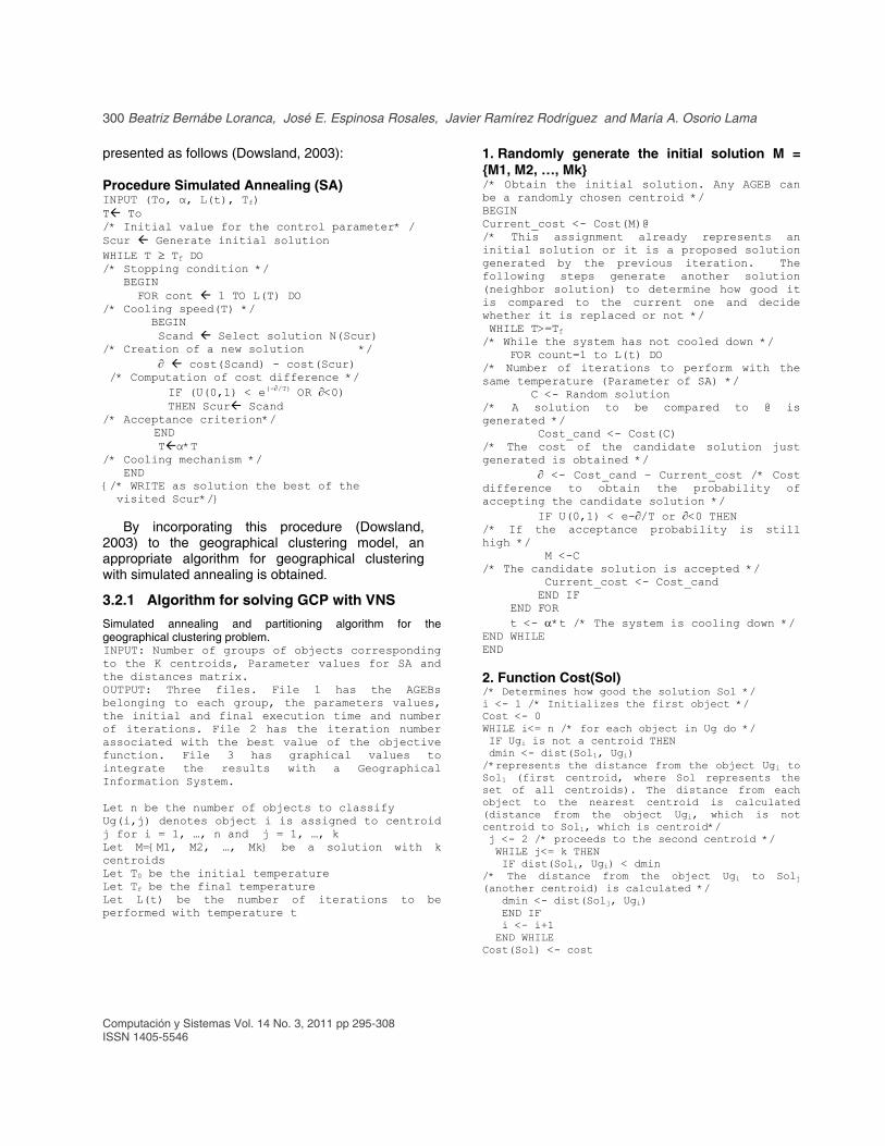
In order to approach the comparative analysis, the VNS experiment reported previously has been revisited (Bernábe, 2009a). The parameter controls for VNS are: neighborhood structures (NS), local search iterations (LS) and the number of groups (G). The parameter levels used in the experiment can be seen in Table 1.

Table 1. Experimentation Level for VNS

Parameter High Center Low LS 848 530 212 NS 640 400 160 G 24 18 12

In Table 2 we show results for 15 configurations

with VNS. The nomenclature used is: NS, LS, G (Groups that mean territory), and OBJ (Objective Value).

Table 2. Configuration for VNS

Test G LS NS OBJ 1 12 212 400 15.4535 2 24 212 400 10.9011 3 12 848 400 15.1598 4 24 848 400 10.8866 5 12 530 160 15.3206 6 24 530 160 11.0177 7 12 530 640 15.3221 8 24 530 640 10.8371 9 18 212 160 12.8541 10 18 848 160 12.4411 11 18 212 640 12.6957 12 18 848 640 12.4726 13 18 530 400 12.5597 14 18 530 400 12.5667



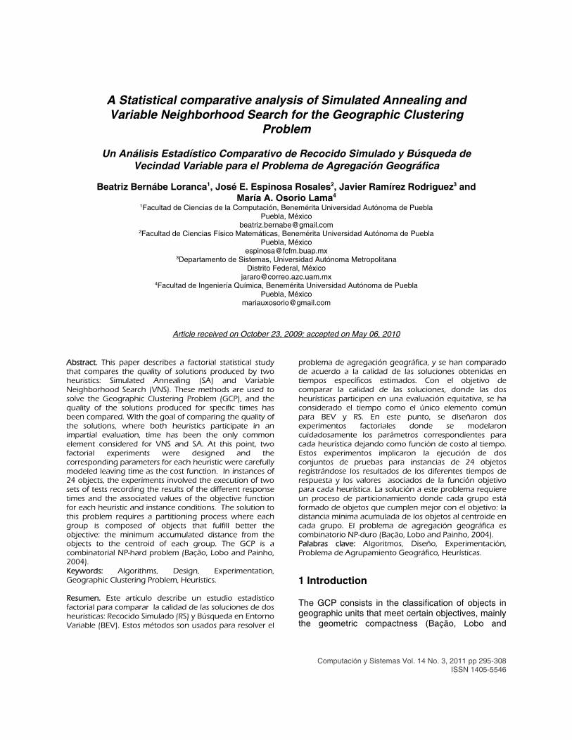
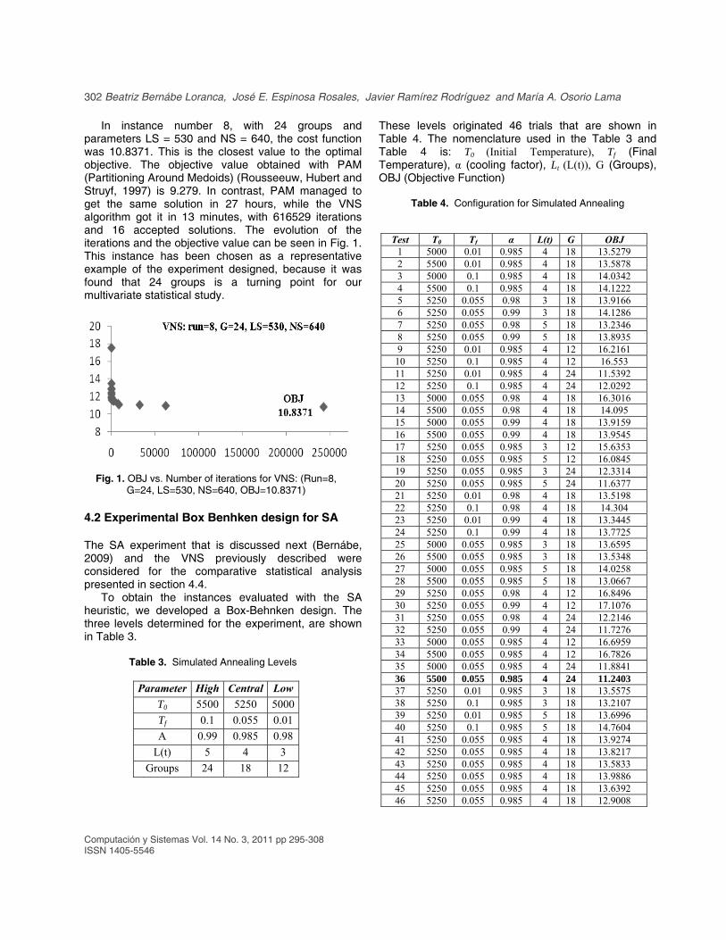
In instance number 8, with 24 groups and parameters LS = 530 and NS = 640, the cost function was 10.8371. This is the closest value to the optimal objective. The objective value obtained with PAM (Partitioning Around Medoids) (Rousseeuw, Hubert and Struyf, 1997) is 9.279. In contrast, PAM managed to get the same solution in 27 hours, while the VNS algorithm got it in 13 minutes, with 616529 iterations and 16 accepted solutions. The evolution of the iterations and the objective value can be seen in Fig. 1. This instance has been chosen as a representative example of the experiment designed, because it was found that 24 groups is a turning point for our multivariate statistical study.

Fig. 1. OBJ vs. Number of iterations for VNS: (Run=8, G=24, LS=530, NS=640, OBJ=10.8371)

4.2 Experimental Box Benhken design for SA

The SA experiment that is discussed next (Bernábe, 2009) and the VNS previously described were considered for the comparative statistical analysis presented in section 4.4.

To obtain the instances evaluated with the SA heuristic, we developed a Box-Behnken design. The three levels determined for the experiment, are shown in Table 3.

Table 3. Simulated Annealing Levels

Parameter High Central Low

T0 5500 5250 5000

Tf 0.1 0.055 0.01

Α 0.99 0.985 0.98

L(t) 5 4 3

Groups 24 18 12

These levels originated 46 trials that are shown in Table 4. The nomenclature used in the Table 3 and Table 4 is: T0 (Initial Temperature), Tf (Final Temperature), α (cooling factor), Lt (L(t)), G (Groups), OBJ (Objective Function)

Table 4. Configuration for Simulated Annealing

Test T0 Tf α L(t) G OBJ 1 5000 0.01 0.985 4 18 13.5279 2 5500 0.01 0.985 4 18 13.5878 3 5000 0.1 0.985 4 18 14.0342 4 5500 0.1 0.985 4 18 14.1222 5 5250 0.055 0.98 3 18 13.9166 6 5250 0.055 0.99 3 18 14.1286 7 5250 0.055 0.98 5 18 13.2346 8 5250 0.055 0.99 5 18 13.8935 9 5250 0.01 0.985 4 12 16.2161 10 5250 0.1 0.985 4 12 16.553 11 5250 0.01 0.985 4 24 11.5392 12 5250 0.1 0.985 4 24 12.0292 13 5000 0.055 0.98 4 18 16.3016 14 5500 0.055 0.98 4 18 14.095 15 5000 0.055 0.99 4 18 13.9159 16 5500 0.055 0.99 4 18 13.9545 17 5250 0.055 0.985 3 12 15.6353 18 5250 0.055 0.985 5 12 16.0845 19 5250 0.055 0.985 3 24 12.3314 20 5250 0.055 0.985 5 24 11.6377 21 5250 0.01 0.98 4 18 13.5198 22 5250 0.1 0.98 4 18 14.304 23 5250 0.01 0.99 4 18 13.3445 24 5250 0.1 0.99 4 18 13.7725 25 5000 0.055 0.985 3 18 13.6595 26 5500 0.055 0.985 3 18 13.5348 27 5000 0.055 0.985 5 18 14.0258 28 5500 0.055 0.985 5 18 13.0667 29 5250 0.055 0.98 4 12 16.8496 30 5250 0.055 0.99 4 12 17.1076 31 5250 0.055 0.98 4 24 12.2146 32 5250 0.055 0.99 4 24 11.7276 33 5000 0.055 0.985 4 12 16.6959 34 5500 0.055 0.985 4 12 16.7826 35 5000 0.055 0.985 4 24 11.8841 36 5500 0.055 0.985 4 24 11.2403 37 5250 0.01 0.985 3 18 13.5575 38 5250 0.1 0.985 3 18 13.2107 39 5250 0.01 0.985 5 18 13.6996 40 5250 0.1 0.985 5 18 14.7604 41 5250 0.055 0.985 4 18 13.9274 42 5250 0.055 0.985 4 18 13.8217 43 5250 0.055 0.985 4 18 13.5833 44 5250 0.055 0.985 4 18 13.9886 45 5250 0.055 0.985 4 18 13.6392 46 5250 0.055 0.985 4 18 12.9008



ISSN 1405-5546

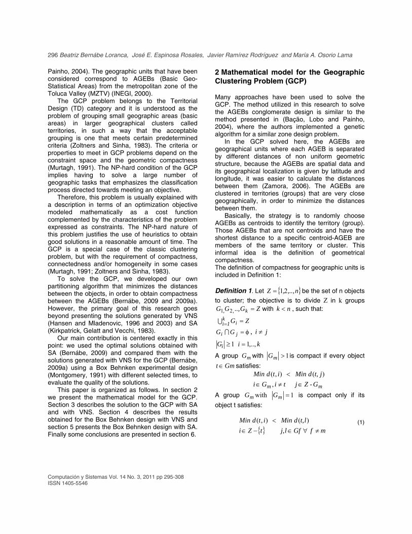
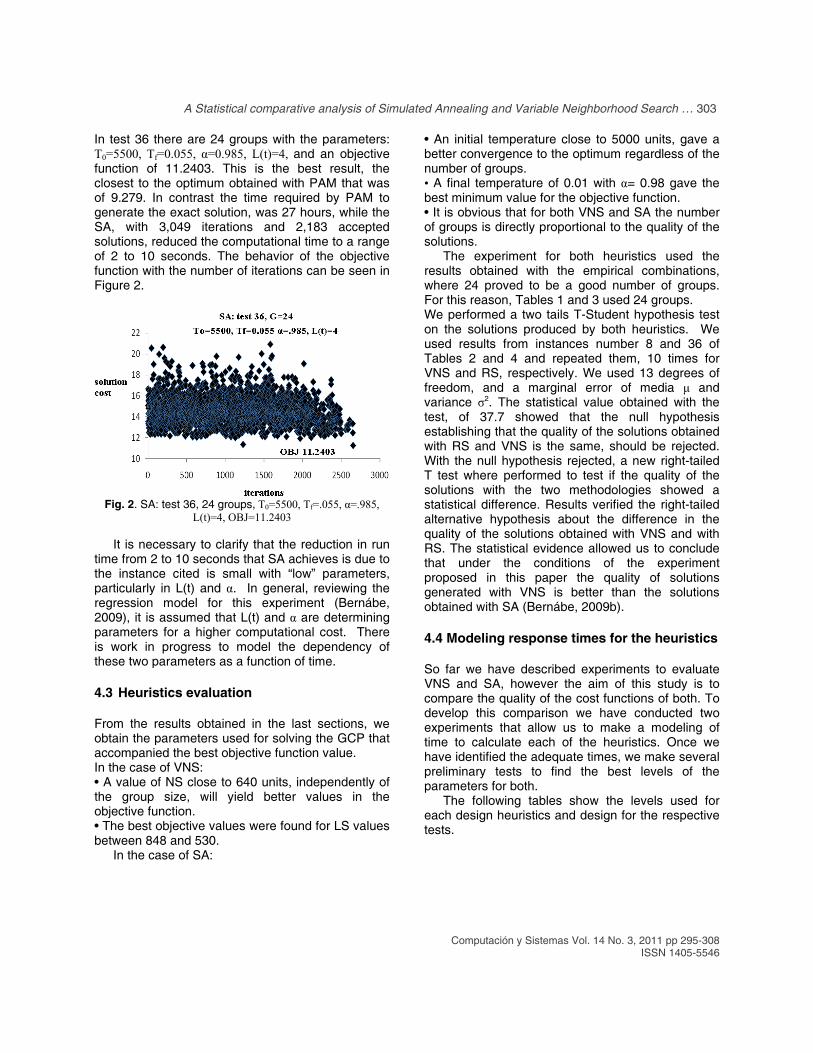
In test 36 there are 24 groups with the parameters: T0=5500, Tf=0.055, α=0.985, L(t)=4, and an objective function of 11.2403. This is the best result, the closest to the optimum obtained with PAM that was of 9.279. In contrast the time required by PAM to generate the exact solution, was 27 hours, while the SA, with 3,049 iterations and 2,183 accepted solutions, reduced the computational time to a range of 2 to 10 seconds. The behavior of the objective function with the number of iterations can be seen in Figure 2.

Fig. 2. SA: test 36, 24 groups, T0=5500, Tf=.055, α=.985,

L(t)=4, OBJ=11.2403

It is necessary to clarify that the reduction in run time from 2 to 10 seconds that SA achieves is due to the instance cited is small with “low” parameters, particularly in L(t) and α. In general, reviewing the regression model for this experiment (Bernábe, 2009), it is assumed that L(t) and α are determining parameters for a higher computational cost. There is work in progress to model the dependency of these two parameters as a function of time.

4.3 Heuristics evaluation

From the results obtained in the last sections, we obtain the parameters used for solving the GCP that accompanied the best objective function value. In the case of VNS: • A value of NS close to 640 units, independently of the group size, will yield better values in the objective function. • The best objective values were found for LS values between 848 and 530. In the case of SA:

• An initial temperature close to 5000 units, gave a better convergence to the optimum regardless of the number of groups. • A final temperature of 0.01 with α= 0.98 gave the best minimum value for the objective function. • It is obvious that for both VNS and SA the number of groups is directly proportional to the quality of the solutions. The experiment for both heuristics used the results obtained with the empirical combinations, where 24 proved to be a good number of groups. For this reason, Tables 1 and 3 used 24 groups. We performed a two tails T-Student hypothesis test on the solutions produced by both heuristics. We used results from instances number 8 and 36 of Tables 2 and 4 and repeated them, 10 times for VNS and RS, respectively. We used 13 degrees of freedom, and a marginal error of media μ and variance σ2. The statistical value obtained with the test, of 37.7 showed that the null hypothesis establishing that the quality of the solutions obtained with RS and VNS is the same, should be rejected. With the null hypothesis rejected, a new right-tailed T test where performed to test if the quality of the solutions with the two methodologies showed a statistical difference. Results verified the right-tailed alternative hypothesis about the difference in the quality of the solutions obtained with VNS and with RS. The statistical evidence allowed us to conclude that under the conditions of the experiment proposed in this paper the quality of solutions generated with VNS is better than the solutions obtained with SA (Bernábe, 2009b).

4.4 Modeling response times for the heuristics

So far we have described experiments to evaluate VNS and SA, however the aim of this study is to compare the quality of the cost functions of both. To develop this comparison we have conducted two experiments that allow us to make a modeling of time to calculate each of the heuristics. Once we have identified the adequate times, we make several preliminary tests to find the best levels of the parameters for both.

The following tables show the levels used for each design heuristics and design for the respective tests.



4.4.1 Modeling response times for VNS

Taking the results from section 4.1, a new set of 35 random duplicates (instances) to build a central composite design since only two parameters are calibrated as a cost function (Montgomery, 1991). Table 5 shows the composed design levels for VNS and Table 6, the experiments performed with VNS. The factorial experiments require the test to be performed to be random, “Standard Order”, tables 6 and 8 show the order in which the test were performed.

Table 5. Composite design levels for VNS

Parameter High Low

LS 916 158

NS 1092 190

Table 6. Configuration for VNS according to

the experimental design

Test Standard Order NS LS T 1 13 641 537 314 2 12 641 537 314 3 4 1092 916 509 4 9 641 537 312 5 8 641 1073 313 6 6 1279 537 624 7 7 641 101 130 8 10 641 537 318 9 3 190 916 90

10 11 641 537 287 11 1 190 158 90 12 2 1092 158 1050 13 5 3.19 537 3

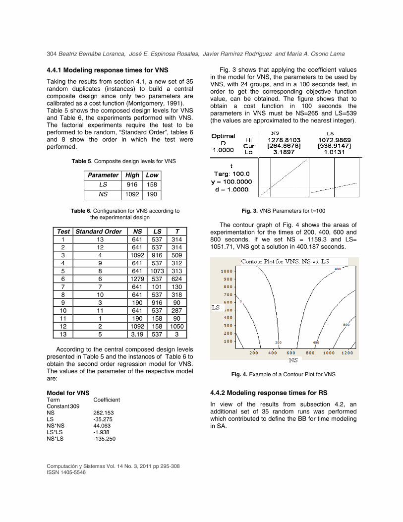
According to the central composed design levels presented in Table 5 and the instances of Table 6 to obtain the second order regression model for VNS. The values of the parameter of the respective model are: Model for VNS Term Coefficient Constant 309 NS 282.153 LS -35.275 NS*NS 44.063 LS*LS -1.938 NS*LS -135.250

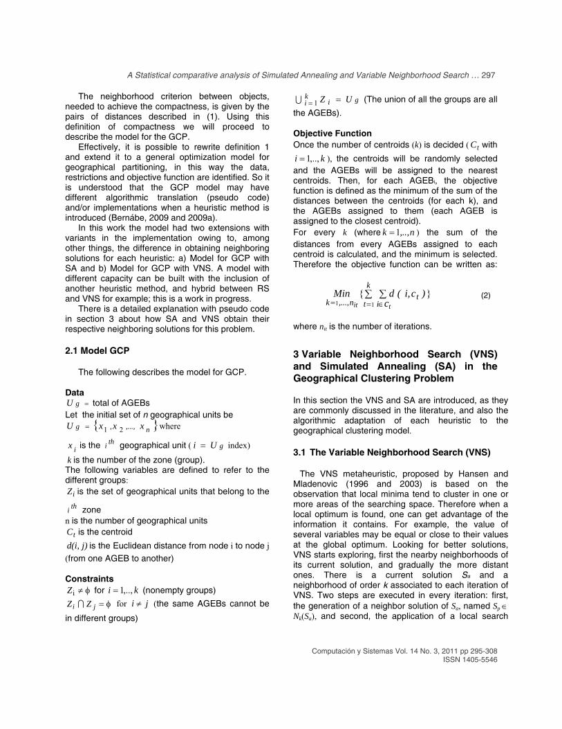
Fig. 3 shows that applying the coefficient values in the model for VNS, the parameters to be used by VNS, with 24 groups, and in a 100 seconds test, in order to get the corresponding objective function value, can be obtained. The figure shows that to obtain a cost function in 100 seconds the parameters in VNS must be NS=265 and LS=539 (the values are approximated to the nearest integer).

Fig. 3. VNS Parameters for t=100 The contour graph of Fig. 4 shows the areas of experimentation for the times of 200, 400, 600 and 800 seconds. If we set NS = 1159.3 and LS= 1051.71, VNS got a solution in 400.187 seconds.

Fig. 4. Example of a Contour Plot for VNS

4.4.2 Modeling response times for RS

In view of the results from subsection 4.2, an additional set of 35 random runs was performed which contributed to define the BB for time modeling in SA.



ISSN 1405-5546

Tables 7 and 8 show a series of tests that respond to the design and the experiments performed with SA.

Table 7. Box Benhken levels for SA

Parameter High Low

T0 50000 500

Tf 0.1 0.01

α 0.99 0.98

L(t) 1000 5

Table 8. Configuration for Simulated Annealing according

to the experimental design

Test

Std. Order T0 Tf α Lt t

1 5 25250 0.055 0.98 5 2 2 2 50000 0.01 0.985 502.5 174 3 10 50000 0.055 0.98 502.5 119 4 14 25250 0.1 0.985 5 3 5 13 25250 0.01 0.985 5 1 6 16 25250 0.1 0.985 1000 285 7 17 500 0.055 0.985 5 2 8 27 25250 0.055 0.985 502.5 154 9 22 25250 0.1 0.98 502.5 129

10 6 25250 0.055 0.99 5 2 11 7 25250 0.055 0.98 1000 219 12 4 50000 0.1 0.985 502.5 150 13 12 50000 0.055 0.99 502.5 239 14 19 500 0.055 0.985 1000 209 15 23 25250 0.01 0.99 502.5 262 16 15 25250 0.01 0.985 1000 354 17 21 25250 0.01 0.98 502.5 126 18 3 500 0.1 0.985 502.5 96 19 25 25250 0.055 0.985 502.5 156 20 8 25250 0.055 0.99 1000 444 21 1 500 0.01 0.985 502.5 125 22 11 500 0.055 0.99 502.5 158 23 18 50000 0.055 0.985 5 2 24 24 25250 0.1 0.99 502.5 217 25 20 50000 0.055 0.985 1000 313 26 9 500 0.055 0.98 502.5 76 27 26 25250 0.055 0.985 502.5 152

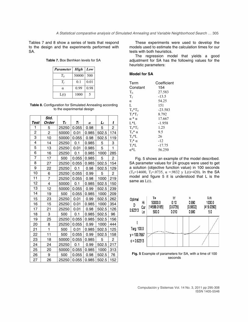
These experiments were used to develop the models used to estimate the calculation times for our tests with both heuristics. The regression model that yields a good adjustment for SA has the following values for the heuristic parameters: Model for SA Term Coefficient Constant 154 T0 27.583 Tf -13.5 α 54.25 L 151 T0*T0 -23.583 Tf*Tf 8.792 α * α 17.667 L*L -1.958 T0*Tf 1.25 T0* α 9.5 T0*L 26 Tf* α -12 Tf*L -17.75 α*L 56.250 Fig. 5 shows an example of the model described. SA parameter values for 24 groups were used to get a solution (objective function value) in 100 seconds (T0=14600, Tf=.0735, α =.9832 y L(t)=420). In the SA model and figure 5 it is understood that L is the same as L(t).

Fig. 5 Example of parameters for SA, with a time of 100 seconds



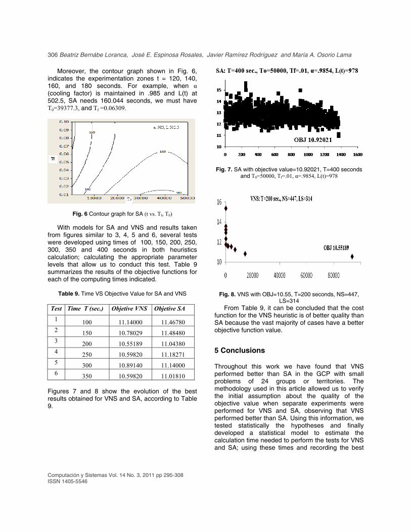
Moreover, the contour graph shown in Fig. 6, indicates the experimentation zones t = 120, 140, 160, and 180 seconds. For example, when α (cooling factor) is maintained in .985 and L(t) at 502.5, SA needs 160.044 seconds, we must have T0=39377.3, and Tf =0.06309.

Fig. 6 Contour graph for SA (t vs. Tf, T0)

With models for SA and VNS and results taken from figures similar to 3, 4, 5 and 6, several tests were developed using times of 100, 150, 200, 250, 300, 350 and 400 seconds in both heuristics calculation; calculating the appropriate parameter levels that allow us to conduct this test. Table 9 summarizes the results of the objective functions for each of the computing times indicated.

Table 9. Time VS Objective Value for SA and VNS

Test Time T (sec.) Objetive VNS Objetive SA

1 100 11.14000 11.46780 2 150 10.78029 11.48480 3 200 10.55189 11.04380 4 250 10.59820 11.18271 5 300 10.89140 11.14000 6 350 10.59820 11.01810

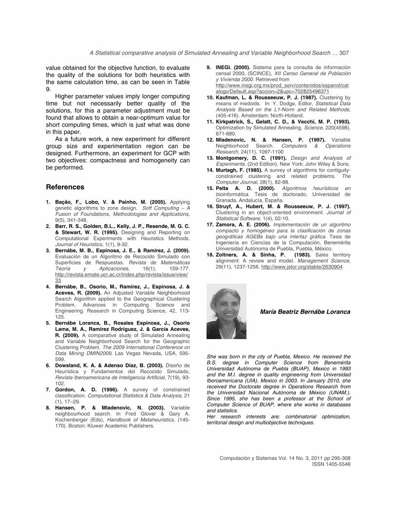
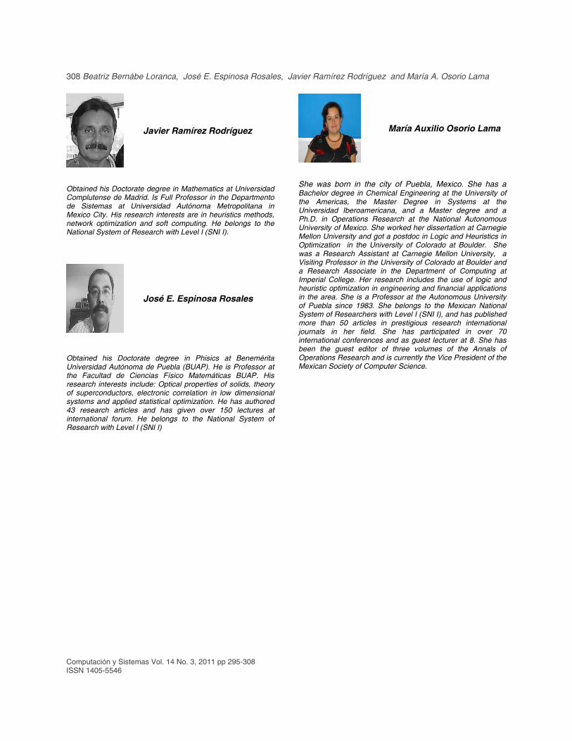
Figures 7 and 8 show the evolution of the best results obtained for VNS and SA, according to Table 9.

Fig. 7. SA with objective value=10.92021, T=400 seconds

and T0=50000, Tf=.01, α=.9854, L(t)=978

Fig. 8. VNS with OBJ=10.55, T=200 seconds, NS=447, LS=314

From Table 9, it can be concluded that the cost function for the VNS heuristic is of better quality than SA because the vast majority of cases have a better objective function value.

5 Conclusions

Throughout this work we have found that VNS performed better than SA in the GCP with small problems of 24 groups or territories. The methodology used in this article allowed us to verify the initial assumption about the quality of the objective value when separate experiments were performed for VNS and SA, observing that VNS performed better than SA. Using this information, we tested statistically the hypotheses and finally developed a statistical model to estimate the calculation time needed to perform the tests for VNS and SA; using these times and recording the best



ISSN 1405-5546

value obtained for the objective function, to evaluate the quality of the solutions for both heuristics with the same calculation time, as can be seen in Table 9. Higher parameter values imply longer computing time but not necessarily better quality of the solutions, for this a parameter adjustment must be found that allows to obtain a near-optimum value for short computing times, which is just what was done in this paper. As a future work, a new experiment for different group size and experimentation region can be designed. Furthermore, an experiment for GCP with two objectives: compactness and homogeneity can be performed.

References

1. Bação, F., Lobo, V. & Painho, M. (2005). Applying genetic algorithms to zone design. Soft Computing – A Fusion of Foundations, Methodologies and Applications, 9(5), 341-348.

2. Barr, R. S., Golden, B.L., Kelly, J. P., Resende, M. G. C. & Stewart, W. R. (1995). Designing and Reporting on Computational Experiments with Heuristics Methods. Journal of Heuristics, 1(1), 9-32.

3. Bernábe, M. B., Espinosa, J. E., & Ramírez, J. (2009). Evaluación de un Algoritmo de Recocido Simulado con Superficies de Respuestas. Revista de Matemáticas Teoría y Aplicaciones, 16(1), 159-177. http://revista.emate.ucr.ac.cr/index.php/revista/issue/view/33

4. Bernábe, B., Osorio, M., Ramírez, J., Espinosa, J. & Aceves, R. (2009). An Adjusted Variable Neighborhood Search Algorithm applied to the Geographical Clustering Problem. Advances in Computing Science and Engineering. Research in Computing Science, 42, 113-125.

5. Bernábe Loranca, B., Rosales Espinosa, J., Osorio Lama, M. A., Ramírez Rodríguez, J. & García Aceves, R. (2009). A comparative study of Simulated Annealing and Variable Neighborhood Search for the Geographic Clustering Problem. The 2009 International Conference on Data Mining DMIN2009, Las Vegas Nevada, USA, 595-599.

6. Dowsland, K. A. & Adenso Díaz, B. (2003). Diseño de Heurística y Fundamentos del Recocido Simulado, Revista Iberoamericana de Inteligencia Artificial, 7(19), 93-102.

7. Gordon, A. D. (1996). A survey of constrained classification. Computational Statistics & Data Analysis, 21 (1), 17–29.

8. Hansen, P. & Mladenovic, N. (2003). Variable neighbourhood search. In Fred Glover & Gary A. Kochenberger (Eds), Handbook of Metaheuristics, (145-170). Boston: Kluwer Academic Publishers.

9. INEGI. (2000). Sistema para la consulta de información censal 2000, (SCINCE), XII Censo General de Población y Vivienda 2000. Retrieved from http://www.inegi.org.mx/prod_serv/contenidos/espanol/catalogo/Default.asp?accion=2&upc=702825496371

10. Kaufman, L. & Rousseeuw, P. J. (1987). Clustering by means of medoids. In: Y. Dodge, Editor, Statistical Data Analysis Based on the L1-Norm and Related Methods, (405-416). Amsterdam: North-Holland.

11. Kirkpatrick, S., Gelatt, C. D., & Vecchi, M. P. (1993). Optimization by Simulated Annealing. Science, 220(4598), 671-680.

12. Mladenovic, N. & Hansen, P. (1997). Variable Neighborhood Search. Computers & Operations Research, 24(11), 1097-1100

13. Montgomery, D. C. (1991). Design and Analysis of Experiments. (2nd Edition). New York: John Wiley & Sons.

14. Murtagh, F. (1985). A survey of algorithms for contiguity-constrained clustering and related problems. The Computer Journal, 28(1), 82-88.

15. Pelta A. D. (2000). Algoritmos heurísticos en bioinformática. Tesis de doctorado, Universidad de Granada, Andalucía, España.

16. Struyf, A., Hubert, M. & Rousseeuw, P. J. (1997). Clustering in an object-oriented environment. Journal of Statistical Software, 1(4), 02-10.

17. Zamora, A. E. (2006). Implementación de un algoritmo compacto y homogéneo para la clasificación de zonas geográficas AGEBs bajo una interfaz gráfica. Tesis de Ingeniería en Ciencias de la Computación, Benemérita Universidad Autónoma de Puebla, Puebla, México.

18. Zoltners, A. & Sinha, P. (1983). Sales territory alignment: A review and model. Management Science, 29(11), 1237-1256. http://www.jstor.org/stable/2630904

María Beatriz Bernábe Loranca

She was born in the city of Puebla, Mexico. He received the B.S. degree in Computer Science from Benemérita Universidad Autónoma de Puebla (BUAP), Mexico in 1993 and the M.I. degree in quality engineering from Universidad Iberoamericana (UIA), Mexico in 2003. In January 2010, she received the Doctorate degree in Operations Research from the Universidad Nacional Autónoma de México (UNAM.). Since 1995, she has been a professor at the School of Computer Science of BUAP, where she works in databases and statistics. Her research interests are: combinatorial optimization, territorial design and multiobjective techniques.



Javier Ramírez Rodríguez

Obtained his Doctorate degree in Mathematics at Universidad Complutense de Madrid. Is Full Professor in the Departmento de Sistemas at Universidad Autónoma Metropolitana in Mexico City. His research interests are in heuristics methods, network optimization and soft computing. He belongs to the National System of Research with Level I (SNI I).

José E. Espinosa Rosales

Obtained his Doctorate degree in Phisics at Benemérita Universidad Autónoma de Puebla (BUAP). He is Professor at the Facultad de Ciencias Físico Matemáticas BUAP. His research interests include: Optical properties of solids, theory of superconductors, electronic correlation in low dimensional systems and applied statistical optimization. He has authored 43 research articles and has given over 150 lectures at international forum. He belongs to the National System of Research with Level I (SNI I)

María Auxilio Osorio Lama

She was born in the city of Puebla, Mexico. She has a Bachelor degree in Chemical Engineering at the University of the Americas, the Master Degree in Systems at the Universidad Iberoamericana, and a Master degree and a Ph.D. in Operations Research at the National Autonomous University of Mexico. She worked her dissertation at Carnegie Mellon University and got a postdoc in Logic and Heuristics in Optimization in the University of Colorado at Boulder. She was a Research Assistant at Carnegie Mellon University, a Visiting Professor in the University of Colorado at Boulder and a Research Associate in the Department of Computing at Imperial College. Her research includes the use of logic and heuristic optimization in engineering and financial applications in the area. She is a Professor at the Autonomous University of Puebla since 1983. She belongs to the Mexican National System of Researchers with Level I (SNI I), and has published more than 50 articles in prestigious research international journals in her field. She has participated in over 70 international conferences and as guest lecturer at 8. She has been the guest editor of three volumes of the Annals of Operations Research and is currently the Vice President of the Mexican Society of Computer Science.

Documents

A Statistical comparative analysis of Simulated … · A Statistical comparative analysis of Simulated Annealing and Variable Neighborhood Search … 297 Computación y Sistemas Vol