Embed Size (px)
Citation preview
The Electronic Journal of Mathematics and Technology, Volume 9, Number 1, ISSN 1933-2823
A Software Tool to Improve Teaching Numerical
Methods.
María Gómez e-mail: [email protected]
Universidad Autónoma Metropolitana
Cuajimalpa, Distrito Federal, México
Jorge Cervantes e-mail: [email protected]
Universidad Autónoma Metropolitana
Cuajimalpa, Distrito Federal, México
Elsa Báez e-mail: [email protected]
Universidad Autónoma Metropolitana
Cuajimalpa, Distrito Federal, México
Alejandra García e-mail: [email protected]
Universidad Autónoma Metropolitana
Cuajimalpa, Distrito Federal, México
Rogelio Ramos e-mail: [email protected]
Universidad Nacional Autónoma de México
Cuautitlán Izcalli, Edo. Mex., México
Abstract We describe and evaluate an educational software tool called Educational Active SYstem for
Numerical Methods (EASyNuM) which provides teaching support for undergraduate courses of
numerical methods. We show our teaching experience results using several tests on a group of
students in order to obtain evidence of the advantages of using this tool. Tests results suggest that,
using the system, students understand better some of the concepts. We also show students’ opinion
through their answers to some questions related to their experience with the system.
.
1. Introduction Numerical Methods is a regular course for engineers and mathematicians. There is a wealth of
resources to support learning numerical methods [6] and online courses [8]. However, when it
comes to demonstrating why numerical methods work, most of these resources use commercial
software such as Mathematica and Maple, which require programming skills and sometimes hinder
understanding how the methods work and the possibility of comparing methods in simple
parameters such as number of iterations.
Some efforts have been undertaken to develop more user friendly software which make
emphasis on understanding the numerical methods, for example, in [3] a tool called CoNum is
described as numerical computation educational software. It is available online at
The Electronic Journal of Mathematics and Technology, Volume 9, Number 1, ISSN 1933-2823
108
http://www.norg.uminho.pt/emgpf/lectivas.htm. However, before CoNum can be used, it requires a
previous installation which is not easy and even not always possible. There is also a tool to learn
approximation and interpolation algorithms commonly used in engineering design published by
Gutiérrez de Ravè et al. [5], called Approximation and Interpolation algorithms. However, the
authors did not make it available to the web. Owens et al. [9] assessed online resources used for an
the engineering course in numerical methods and demonstrated that website modules can be very
helpful. They analyzed specifically a very complete, award winning, online resource for an
undergraduate course in numerical methods [6-7].
We have developed a system for teaching numerical methods called Educational Active
SYstem for Numerical Methods (EASyNuM). EASyNuM offers teachers a tool to explain some
subtleties in numerical methods and thus students have the opportunity to acquire better
understanding. It is freely available on the web at
http://libio.cua.uam.mx/~coordinacioningcomp/SiMetNum/simv4.html
and very easy to use. With EASyNuM the user can introduce different parameters and see
final results on screen for their analysis. Teachers can work with examples that, when performed
manually, take a lot of time. It can also help in the preparation of exams and class exercises.
One of the main advantages of EASyNuM when compared with other resources is that it has
a parser. With it, students can experiment with several different functions (when needed) in order to
better understand the essence of some methods by checking how results can change depending on
the function that is being used. For example, suppose we want to find some root of a polynomial
function using either Bisection or Newton-Raphson method. After having done several exercises,
students can then be asked to find the root of several functions including some non-polynomials.
This should illustrate the power of the method because, for many of these functions, there might be
no analytical method available for this purpose. Students can then start playing with functions of
their own.
According to Crouch et al. [2] “Science education research shows that most students learn
more from instruction that actively engages them rather than from traditional methods in which they
are passive spectators”. Shacham et al. [10] developed a set of numerical problems and solved them
via computer with active participation of students and discussed the educational benefits of this
approach. Exercises of this kind are called live demonstrations and according to Di Stefano [4] they
stimulate students’ interest. EASyNuM facilitates carrying out live demonstrations of numerical
methods so students get the picture about the methods studied and their operation. EASyNuM was
designed to motivate students to do exploration in order to understand better the way numerical
methods work. It also enhances the development of metacognitive skills which are seen as crucial to
learn [1].
In section 2 we briefly describe EASyNuM and its scope. In section 3 we show how the
system can be used by teachers to show some properties of the methods. Section 4 shows results of
the tests that we have performed to produce evidence of the effects in the students' understanding by
using the system. Conclusions are in Section 5.
2. Scope of EASyNuM It is important to notice that the main purpose of EASyNuM is not to execute numerical methods
quickly, but, rather, to clearly show their properties. The methods that are included in EASyNuM are grouped in four categories:
Solution of Non-Linear Equations:
o Newton-Raphson and
o Bisection.
The Electronic Journal of Mathematics and Technology, Volume 9, Number 1, ISSN 1933-2823
109
Systems of Linear Equations:
o Jacobi and
o Gauss-Seidel.
Interpolation:
o Newton’s forward interpolation and
o Lagrange’s Interpolation.
Numerical Integration:
o Composite Trapezoidal,
o Composite Simpson’s 1/3 rule, and
o Composite Simpson’s 3/8 rule.
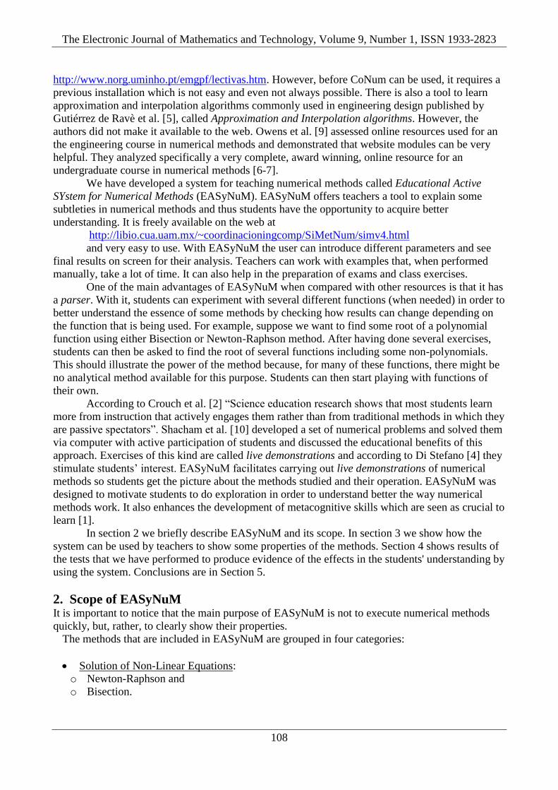
Fig. 1 shows the EASyNuM home page. The user must pass the mouse over one of the
groups of methods in order to see the methods' list.
Figure 1: EASyNuM home page
The current version of the system is in Spanish and all the implemented numerical methods
have the same format which consists of three parts: a brief description of the method, the user
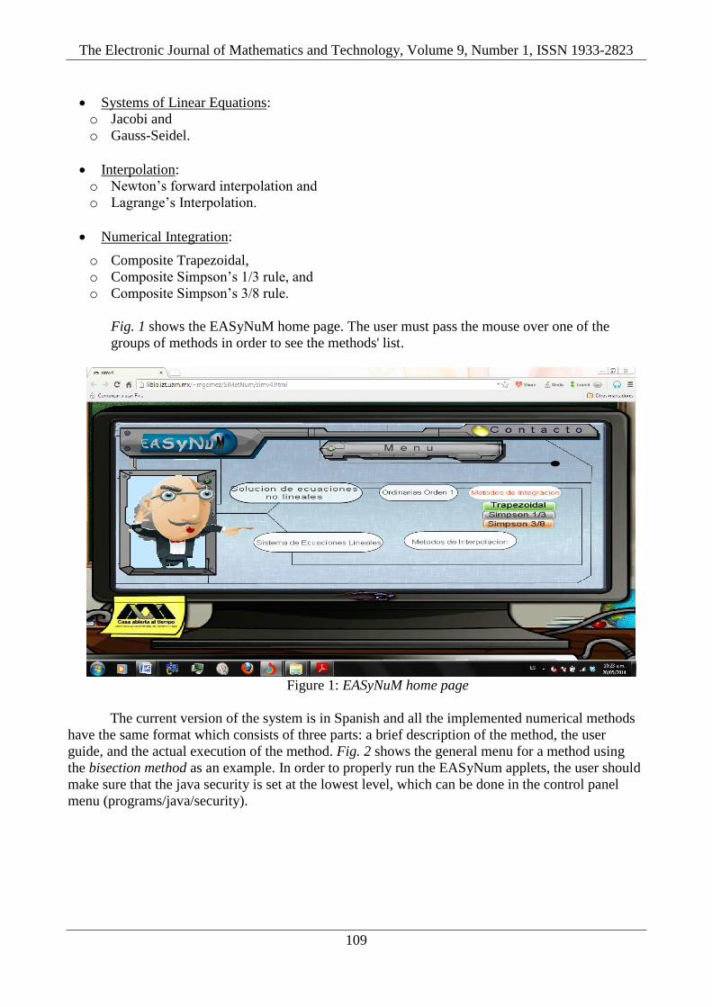
guide, and the actual execution of the method. Fig. 2 shows the general menu for a method using
the bisection method as an example. In order to properly run the EASyNum applets, the user should
make sure that the java security is set at the lowest level, which can be done in the control panel
menu (programs/java/security).
The Electronic Journal of Mathematics and Technology, Volume 9, Number 1, ISSN 1933-2823
110
Figure 2: Bisection method page
3. Learning some properties of the numerical methods with EASyNuM
3.1. Speed of iterative methods
Teaching how many iterations a method would require to achieve an accuracy (tolerance) given,
as well as the aspects which depend on the convergence of the problem, is not an easy task and
consumes a lot of effort in the classroom. However EASyNuM provides results that illustrate in a
didactic way, all these aspects. Students can easily and see, for example, how sensitive is the
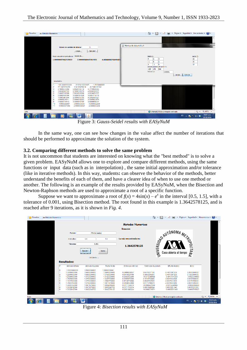
number of iterations to changes in some parameter. As an example, we can use the Gauss-Seidel
method to find the solution of the following system of linear equations:
23
30
22
611
281
126
3
2
1
x
x
x
with the initial solution vector x(0) = [0, 0, 0]T and a tolerance of 0.00001. EASyNuM gives the
approximate solution (2.00000, 3.00000, 4.00000) after 8 iterations. If the initial solution vector is
replaced by x(0) = [-255, 170, 800]T students can see that only 11 iterations are required to obtain a
solution within the same tolerance. Student can see that, in some cases, the Gauss-Seidel method
converges quickly even if the initial solution vector is very far from the exact solution. Fig. 3 shows
an screenshot of the results given by EASyNuM.
The Electronic Journal of Mathematics and Technology, Volume 9, Number 1, ISSN 1933-2823
111
Figure 3: Gauss-Seidel results with EASyNuM
In the same way, one can see how changes in the value affect the number of iterations that
should be performed to approximate the solution of the system.
3.2. Comparing different methods to solve the same problem
It is not uncommon that students are interested on knowing what the "best method" is to solve a
given problem. EASyNuM allows one to explore and compare different methods, using the same
functions or input data (such as in interpolation) , the same initial approximation and/or tolerance
(like in iterative methods). In this way, students: can observe the behavior of the methods, better
understand the benefits of each of them, and have a clearer idea of when to use one method or
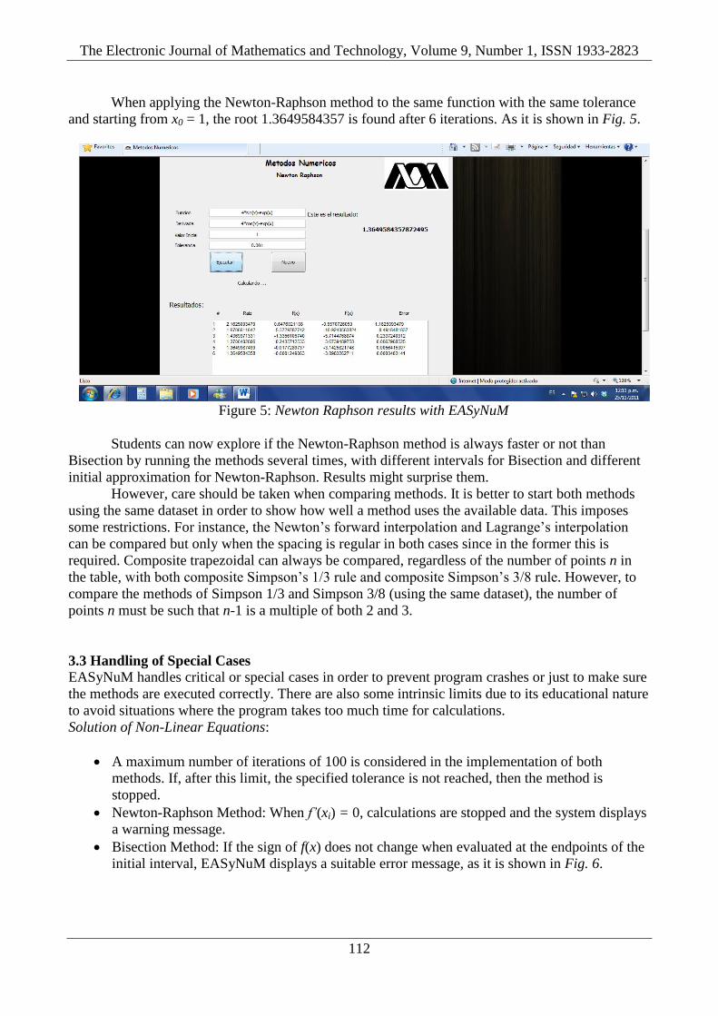
another. The following is an example of the results provided by EASyNuM, when the Bisection and
Newton-Raphson methods are used to approximate a root of a specific function.
Suppose we want to approximate a root of f(x) = 4sin(x) – ex in the interval [0.5, 1.5], with a
tolerance of 0.001, using Bisection method. The root found in this example is 1.3642578125, and is
reached after 9 iterations, as it is shown in Fig. 4.
Figure 4: Bisection results with EASyNuM
The Electronic Journal of Mathematics and Technology, Volume 9, Number 1, ISSN 1933-2823
112
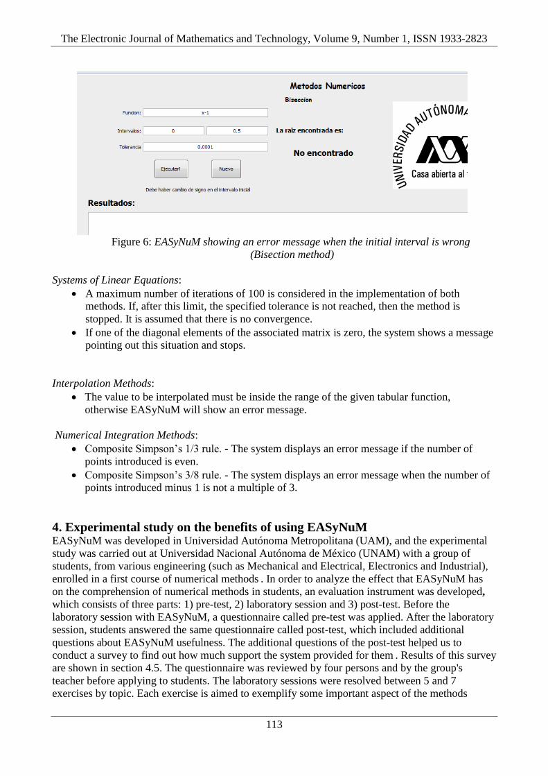
When applying the Newton-Raphson method to the same function with the same tolerance
and starting from x0 = 1, the root 1.3649584357 is found after 6 iterations. As it is shown in Fig. 5.
Figure 5: Newton Raphson results with EASyNuM
Students can now explore if the Newton-Raphson method is always faster or not than
Bisection by running the methods several times, with different intervals for Bisection and different
initial approximation for Newton-Raphson. Results might surprise them.
However, care should be taken when comparing methods. It is better to start both methods
using the same dataset in order to show how well a method uses the available data. This imposes
some restrictions. For instance, the Newton’s forward interpolation and Lagrange’s interpolation
can be compared but only when the spacing is regular in both cases since in the former this is
required. Composite trapezoidal can always be compared, regardless of the number of points n in
the table, with both composite Simpson’s 1/3 rule and composite Simpson’s 3/8 rule. However, to
compare the methods of Simpson 1/3 and Simpson 3/8 (using the same dataset), the number of
points n must be such that n-1 is a multiple of both 2 and 3.
3.3 Handling of Special Cases EASyNuM handles critical or special cases in order to prevent program crashes or just to make sure
the methods are executed correctly. There are also some intrinsic limits due to its educational nature
to avoid situations where the program takes too much time for calculations.
Solution of Non-Linear Equations:
A maximum number of iterations of 100 is considered in the implementation of both
methods. If, after this limit, the specified tolerance is not reached, then the method is
stopped.
Newton-Raphson Method: When f’(xi) = 0, calculations are stopped and the system displays
a warning message.
Bisection Method: If the sign of f(x) does not change when evaluated at the endpoints of the
initial interval, EASyNuM displays a suitable error message, as it is shown in Fig. 6.
The Electronic Journal of Mathematics and Technology, Volume 9, Number 1, ISSN 1933-2823
113
Figure 6: EASyNuM showing an error message when the initial interval is wrong
(Bisection method)
Systems of Linear Equations:
A maximum number of iterations of 100 is considered in the implementation of both
methods. If, after this limit, the specified tolerance is not reached, then the method is
stopped. It is assumed that there is no convergence.
If one of the diagonal elements of the associated matrix is zero, the system shows a message
pointing out this situation and stops.
Interpolation Methods:
The value to be interpolated must be inside the range of the given tabular function,
otherwise EASyNuM will show an error message.
Numerical Integration Methods:
Composite Simpson’s 1/3 rule. - The system displays an error message if the number of
points introduced is even.
Composite Simpson’s 3/8 rule. - The system displays an error message when the number of
points introduced minus 1 is not a multiple of 3.
4. Experimental study on the benefits of using EASyNuM EASyNuM was developed in Universidad Autónoma Metropolitana (UAM), and the experimental
study was carried out at Universidad Nacional Autónoma de México (UNAM) with a group of
students, from various engineering (such as Mechanical and Electrical, Electronics and Industrial),
enrolled in a first course of numerical methods . In order to analyze the effect that EASyNuM has
on the comprehension of numerical methods in students, an evaluation instrument was developed,
which consists of three parts: 1) pre-test, 2) laboratory session and 3) post-test. Before the
laboratory session with EASyNuM, a questionnaire called pre-test was applied. After the laboratory
session, students answered the same questionnaire called post-test, which included additional
questions about EASyNuM usefulness. The additional questions of the post-test helped us to
conduct a survey to find out how much support the system provided for them . Results of this survey
are shown in section 4.5. The questionnaire was reviewed by four persons and by the group's
teacher before applying to students. The laboratory sessions were resolved between 5 and 7
exercises by topic. Each exercise is aimed to exemplify some important aspect of the methods
The Electronic Journal of Mathematics and Technology, Volume 9, Number 1, ISSN 1933-2823
114
studied for the subject matter. The questionnaires contain some multiple choice questions, others
can choose between two options ("true" or "false"), and there are also some others in which students
are required to write the answer. In each laboratory session we tried to cover the most relevant
aspects of each set of methods, paying special attention to subtleties involved such as number of
iterations, convergence, etc. Each laboratory session lasted 2 hours and they were undertaken 3
weeks apart.
In the next subsections we present the results of the evaluation instruments for each of the
four categories. These results are presented in two ways: number of correct answers and test score
histogram. The former allows us to see the usefulness of EASyNuM for each question. The latter is
useful to see if students accumulate knowledge by measuring the number of correct answers in the
two questionnaires we evaluated.
For space reasons, only the laboratory session and questionnaire of the evaluation instrument
for the first group of methods are included in Appendix A. For the rest of groups we include results
only. The full set of evaluation instruments of this study can be consulted at the following
addresses:
Systems of linear equations.- https://dl.dropboxusercontent.com/u/
33870917/Systems_of_linear_equations.pdf
Interpolation methods.-
https://dl.dropboxusercontent.com/u/33870917/Interpolation_methods.pdf
Integration methods.-
https://dl.dropboxusercontent.com/u/33870917/Integration_methods.pdf
4.1. Results for Non-Linear Equations
In figure 7a) one can see that the number of correct answers in the post-test, increased in most of
the questions, especially in questions 1.1, 1.2 and 6 (see Appendix A), where the correct answers
grew to more than double after practice with EASyNuM. In the histogram of figure 7b) one can see
that the distribution of test scores is considerably shifted to higher values after the laboratory
session showing that, individually, students improved their understanding of the topic after the
laboratory session .
It can be noticed that EASyNuM is particularly useful to demonstrate the differences
between Bisection and Newton-Raphson methods, as observing the behavior of each method when
different initial intervals are used for the first one, and several initial values (even far from the root)
for the second one.
7a) Number of correct answers per question
The Electronic Journal of Mathematics and Technology, Volume 9, Number 1, ISSN 1933-2823
115
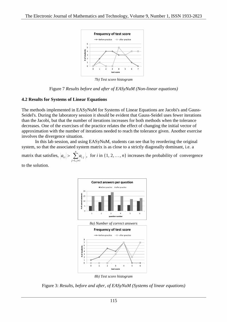
7b) Test score histogram
Figure 7 Results before and after of EASyNuM (Non-linear equations)
4.2 Results for Systems of Linear Equations
The methods implemented in EASyNuM for Systems of Linear Equations are Jacobi's and Gauss-
Seidel's. During the laboratory session it should be evident that Gauss-Seidel uses fewer iterations
than the Jacobi, but that the number of iterations increases for both methods when the tolerance
decreases. One of the exercises of the practice relates the effect of changing the initial vector of
approximation with the number of iterations needed to reach the tolerance given. Another exercise
involves the divergence situation.
In this lab session, and using EASyNuM, students can see that by reordering the original
system, so that the associated system matrix is as close to a strictly diagonally dominant, i.e. a
matrix that satisfies,
n
ijj
jiii aa,1
, for i in {1, 2, , n} increases the probability of convergence
to the solution.
8a) Number of correct answers
8b) Test score histogram
Figure 3: Results, before and after, of EASyNuM (Systems of linear equations)
The Electronic Journal of Mathematics and Technology, Volume 9, Number 1, ISSN 1933-2823
116
Figure 8a) shows that the number of correct answers increased notably after laboratory
session, for all questions, and in figure 8b) we can see a clear improvement in test scores too.
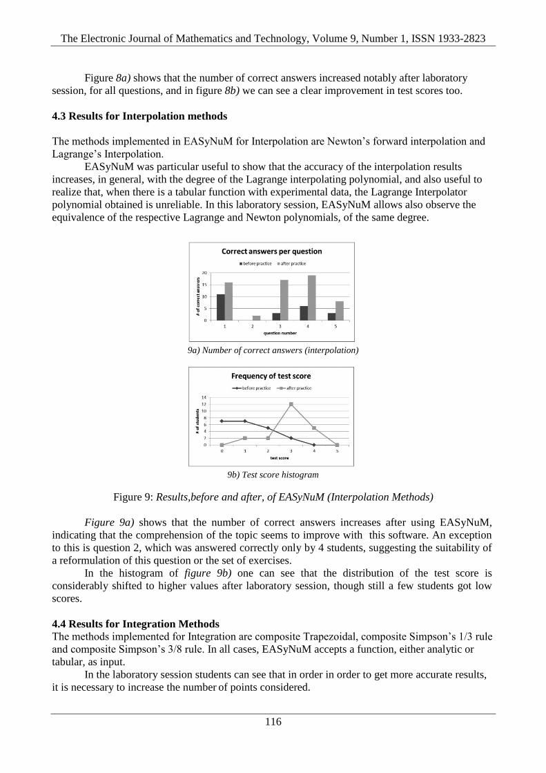
4.3 Results for Interpolation methods
The methods implemented in EASyNuM for Interpolation are Newton’s forward interpolation and
Lagrange’s Interpolation.
EASyNuM was particular useful to show that the accuracy of the interpolation results
increases, in general, with the degree of the Lagrange interpolating polynomial, and also useful to
realize that, when there is a tabular function with experimental data, the Lagrange Interpolator
polynomial obtained is unreliable. In this laboratory session, EASyNuM allows also observe the
equivalence of the respective Lagrange and Newton polynomials, of the same degree.
9a) Number of correct answers (interpolation)
9b) Test score histogram
Figure 9: Results,before and after, of EASyNuM (Interpolation Methods)
Figure 9a) shows that the number of correct answers increases after using EASyNuM,
indicating that the comprehension of the topic seems to improve with this software. An exception
to this is question 2, which was answered correctly only by 4 students, suggesting the suitability of
a reformulation of this question or the set of exercises.
In the histogram of figure 9b) one can see that the distribution of the test score is
considerably shifted to higher values after laboratory session, though still a few students got low
scores.
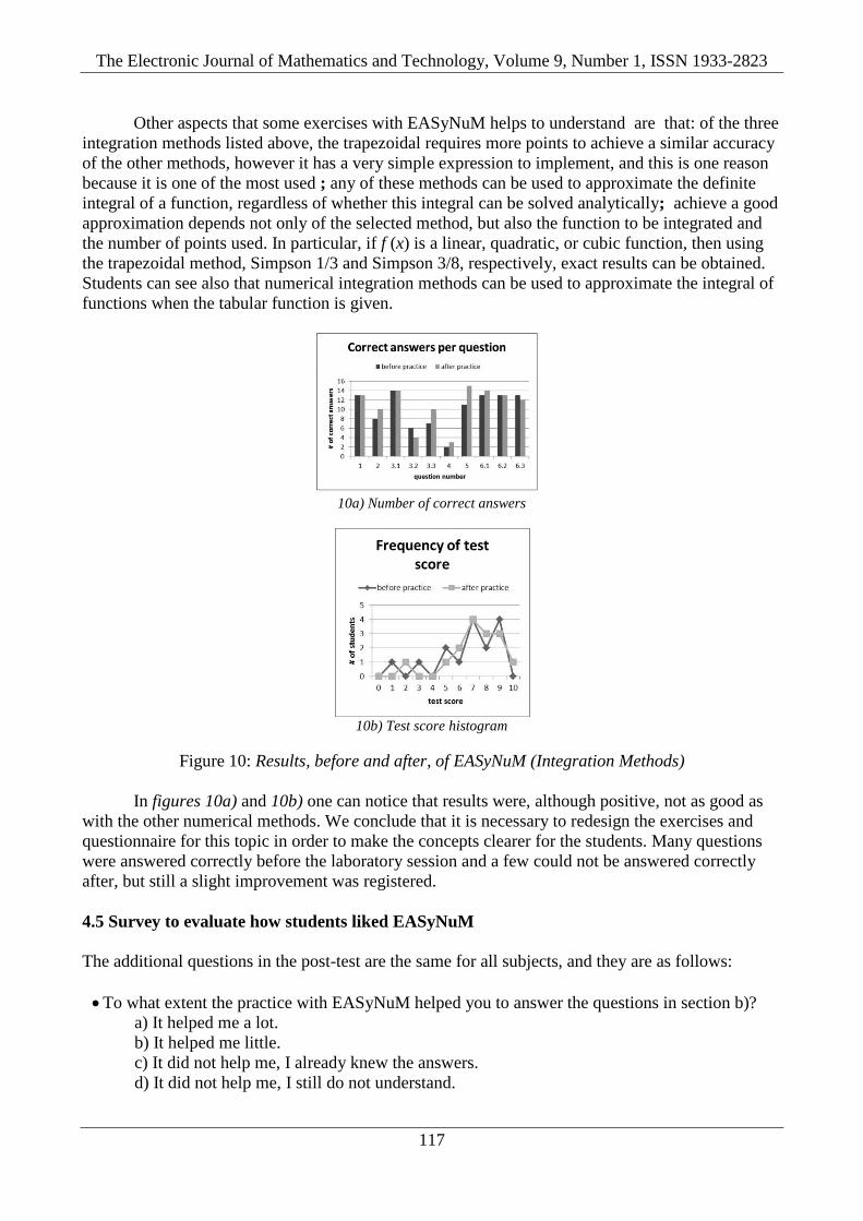
4.4 Results for Integration Methods
The methods implemented for Integration are composite Trapezoidal, composite Simpson’s 1/3 rule
and composite Simpson’s 3/8 rule. In all cases, EASyNuM accepts a function, either analytic or
tabular, as input.
In the laboratory session students can see that in order in order to get more accurate results,
it is necessary to increase the number of points considered.
The Electronic Journal of Mathematics and Technology, Volume 9, Number 1, ISSN 1933-2823
117
Other aspects that some exercises with EASyNuM helps to understand are that: of the three
integration methods listed above, the trapezoidal requires more points to achieve a similar accuracy
of the other methods, however it has a very simple expression to implement, and this is one reason
because it is one of the most used ; any of these methods can be used to approximate the definite
integral of a function, regardless of whether this integral can be solved analytically; achieve a good
approximation depends not only of the selected method, but also the function to be integrated and
the number of points used. In particular, if f (x) is a linear, quadratic, or cubic function, then using
the trapezoidal method, Simpson 1/3 and Simpson 3/8, respectively, exact results can be obtained.
Students can see also that numerical integration methods can be used to approximate the integral of
functions when the tabular function is given.
10a) Number of correct answers
10b) Test score histogram
Figure 10: Results, before and after, of EASyNuM (Integration Methods)
In figures 10a) and 10b) one can notice that results were, although positive, not as good as
with the other numerical methods. We conclude that it is necessary to redesign the exercises and
questionnaire for this topic in order to make the concepts clearer for the students. Many questions
were answered correctly before the laboratory session and a few could not be answered correctly
after, but still a slight improvement was registered.
4.5 Survey to evaluate how students liked EASyNuM
The additional questions in the post-test are the same for all subjects, and they are as follows:
To what extent the practice with EASyNuM helped you to answer the questions in section b)?
a) It helped me a lot.
b) It helped me little.
c) It did not help me, I already knew the answers.
d) It did not help me, I still do not understand.
The Electronic Journal of Mathematics and Technology, Volume 9, Number 1, ISSN 1933-2823
118
Results per laboratory session are shown in Table 1.
Table 1: EASyNuM Usefulness
What aspects of EASyNuM were helpful?
The most important observations are listed below:
o All (37).
o The system shows partial results (8).
o It is easy and fast (11).
o It helps to understand concepts (7).
o The ability to compare methods (5).
What aspects are not suitable?
The most important observations are listed below:
o Entering a function is uncomfortable (10).
o It is necessary to improve the explanation of how to enter functions (3).
o When one needs to introduce fractions, instead of giving the format a/b it is necessary to
give the corresponding decimal number. For example the system accepts only 0.3333 and
not 1/3 (2).
From the survey we observed that the opinion of the students about EASyNuM is very
positive with only a few negative comments. The latter will be considered in the next version of the
system
5. Conclusions EASyNuM is a convenient freely available software software tool, which works on the web, that
provides support for teachers and students. It can be used with any operating system and does not
require any special installation. EASyNuM displays relevant aspects for learning numerical
methods. Particularly it allows the observation of key features of each method, helping students to
build their intuition and, as they have expressed, they appreciate it very much. It has a parser that
allows the system to accept any function as input, including invocations to transcendent functions
making the system very flexible and suitable for exploration. It also facilitates comparisons between
methods solving the same problem.
In addition EASyNuM can help to clarify what happens when some parameters (such as
tolerance or the initial approximation) are introduced.
Finally, EASyNuM helps teachers in creating and assessing tests and assignments. It helps
students to verify their hand calculations, and it can also help advanced students who require a user-
friendly system for solving problems that do not require heavy loads of computing.
The study presented here allowed us to see that, although results are clearly positive, the
exercises included in the laboratory sessions can be improved, and it is also necessary to improve
the development of the test questions. We would strongly support on the suggestion made by
Owens et al.[9] to develop a conceptual inventory on numerical methods. Having such an inventory
would aid comparing different teaching methods.
The Electronic Journal of Mathematics and Technology, Volume 9, Number 1, ISSN 1933-2823
119
EASyNuM can be qualified in general as very useful when teaching numerical methods and
it was also highly appreciated by the students; even those with a low level in programming were
able to understand the methods with minimal effort. Overall, results are very positive and we feel
encouraged to keep using the system in future courses.
8. References [1] Bransford, J., Brown, A. & Cocking, R., (2000), How people learn: brain mind and
transfer, Washington, D.C. National Academies Press.
[2] Crouch C.H., Fagen A.P., Callan J.P., & Mazur E., (2004), Classroom demonstrations:
Learning tools or entertainment?, Am J Phys, 72: 835-838.
[3] Carneiro F., Leão C. P. & Texeira C. F., (2010), Teaching Differential Equations in
Different Environments: A First Approach, Comput Appl in Eng Educ., 18(3): 555-562.
[4] Di Stefano R., (1996), Preliminary IUPP results: Student reactions to in-class
demonstrations and to the presentation of coherent themes, Am J Phys, 64: 58-68.
[5] Gutiérrez de Ravé E., Jiménez-Hornero F. J. & Giráldez J. V., (2011), A Computer
Application for teaching and learning Approximation and Interpolation Algorithms of
Curves, Comput Appl in Eng Educ.,19(1): 40-47.
[6] Holistic Numerical Methods, Transforming Numerical Methods education for
undergraduates. http://numericalmethods.eng.usf.edu, 2009.
[7] Kaw A. K., Collier N., Keteltas M., Paul J. & Besterfield G., (2003) Holistic but customized
resources for a course in Numerical Methods, Comput Appl in Eng Educ, 11: 203-210.
[8] MIT open courseware. http://mit.ocw.edu, 2009.
[9] Owens C., Kaw A., Hess M., (2012), Assessing Online Resources for an Engineering
Course in Numerical Methods, Comput Appl in Eng Educ, 20(3): 426-433.
[10] Shacham M., Cutlip M., Elly M., 2009), Live Problem Solving via Computer in the
Classroom to Avoid Death by Power Point, Comput Appl in Eng Educ, 17:241-252.
The Electronic Journal of Mathematics and Technology, Volume 9, Number 1, ISSN 1933-2823
120
Appendix A: Laboratory session and questionnaire for Non-Linear Equations Results obtained with EASyNuM are marked in grey, correct options are highlighted using bold
font and correct text answers are in italic.
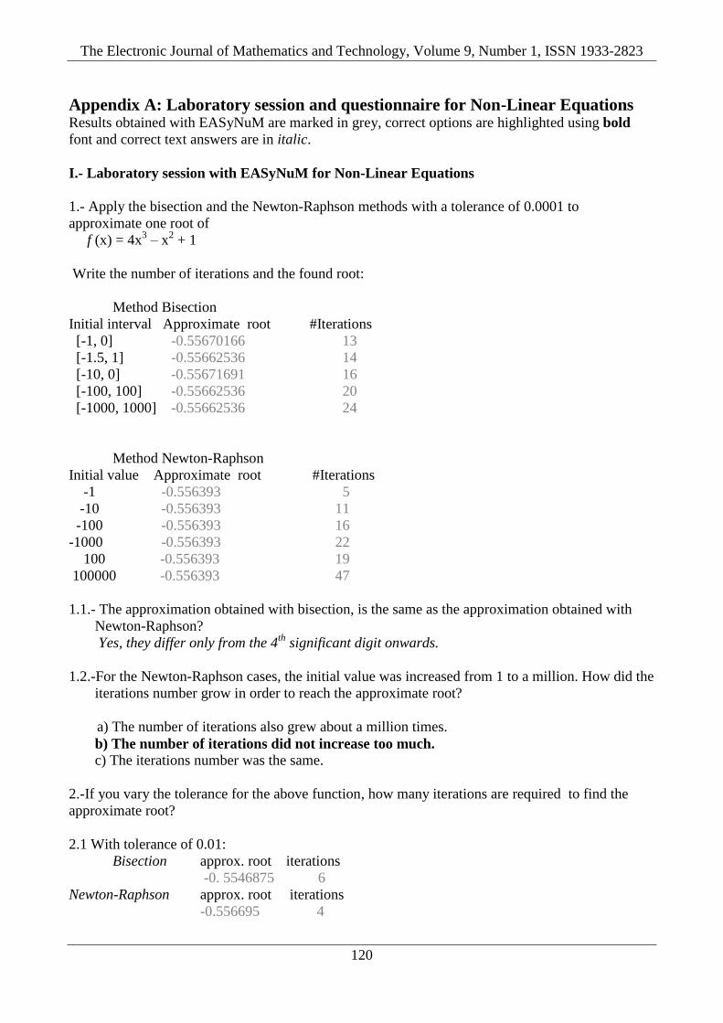
I.- Laboratory session with EASyNuM for Non-Linear Equations
1.- Apply the bisection and the Newton-Raphson methods with a tolerance of 0.0001 to
approximate one root of
f (x) = 4x3 – x
2 + 1
Write the number of iterations and the found root:
Method Bisection
Initial interval Approximate root #Iterations
[-1, 0] -0.55670166 13
[-1.5, 1] -0.55662536 14
[-10, 0] -0.55671691 16
[-100, 100] -0.55662536 20
[-1000, 1000] -0.55662536 24
Method Newton-Raphson
Initial value Approximate root #Iterations
-1 -0.556393 5
-10 -0.556393 11
-100 -0.556393 16
-1000 -0.556393 22
100 -0.556393 19
100000 -0.556393 47
1.1.- The approximation obtained with bisection, is the same as the approximation obtained with
Newton-Raphson?
Yes, they differ only from the 4th
significant digit onwards.
1.2.-For the Newton-Raphson cases, the initial value was increased from 1 to a million. How did the
iterations number grow in order to reach the approximate root?
a) The number of iterations also grew about a million times.
b) The number of iterations did not increase too much. c) The iterations number was the same.
2.-If you vary the tolerance for the above function, how many iterations are required to find the
approximate root?
2.1 With tolerance of 0.01:
Bisection approx. root iterations
-0. 5546875 6
Newton-Raphson approx. root iterations
-0.556695 4
The Electronic Journal of Mathematics and Technology, Volume 9, Number 1, ISSN 1933-2823
121
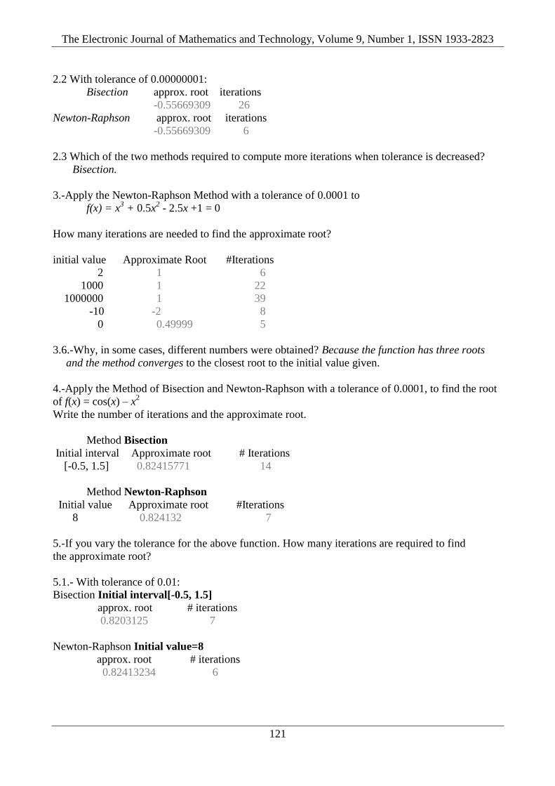
2.2 With tolerance of 0.00000001:
Bisection approx. root iterations
-0.55669309 26
Newton-Raphson approx. root iterations
-0.55669309 6
2.3 Which of the two methods required to compute more iterations when tolerance is decreased?
Bisection.
3.-Apply the Newton-Raphson Method with a tolerance of 0.0001 to
f(x) = x3 + 0.5x
2 - 2.5x +1 = 0
How many iterations are needed to find the approximate root?
initial value Approximate Root #Iterations
2 1 6
1000 1 22
1000000 1 39
-10 -2 8
0 0.49999 5
3.6.-Why, in some cases, different numbers were obtained? Because the function has three roots
and the method converges to the closest root to the initial value given.
4.-Apply the Method of Bisection and Newton-Raphson with a tolerance of 0.0001, to find the root
of f(x) = cos(x) – x2
Write the number of iterations and the approximate root.
Method Bisection
Initial interval Approximate root # Iterations
[-0.5, 1.5] 0.82415771 14
Method Newton-Raphson
Initial value Approximate root #Iterations
8 0.824132 7
5.-If you vary the tolerance for the above function. How many iterations are required to find
the approximate root?
5.1.- With tolerance of 0.01:
Bisection Initial interval[-0.5, 1.5]
approx. root # iterations
0.8203125 7
Newton-Raphson Initial value=8
approx. root # iterations
0.82413234 6
The Electronic Journal of Mathematics and Technology, Volume 9, Number 1, ISSN 1933-2823
122
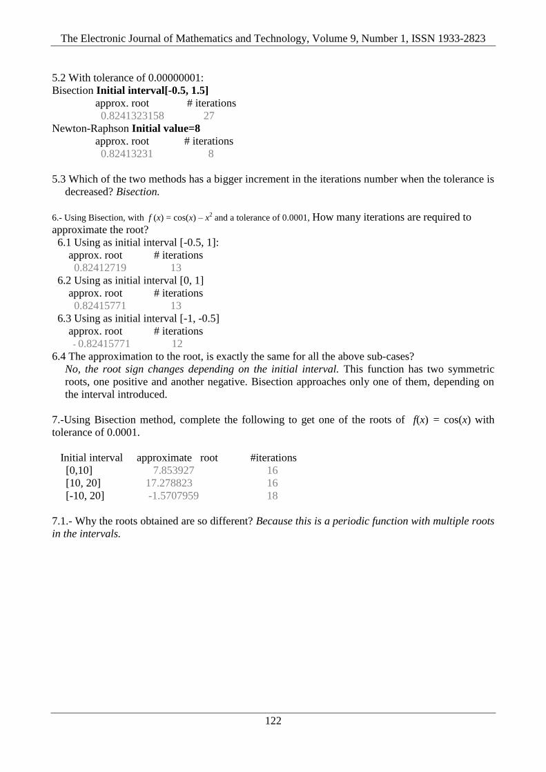
5.2 With tolerance of 0.00000001:
Bisection Initial interval[-0.5, 1.5]
approx. root # iterations
0.8241323158 27
Newton-Raphson Initial value=8
approx. root # iterations
0.82413231 8
5.3 Which of the two methods has a bigger increment in the iterations number when the tolerance is
decreased? Bisection.
6.- Using Bisection, with f (x) = cos(x) – x2 and a tolerance of 0.0001, How many iterations are required to
approximate the root?
6.1 Using as initial interval [-0.5, 1]:
approx. root # iterations
0.82412719 13
6.2 Using as initial interval [0, 1]
approx. root # iterations
0.82415771 13
6.3 Using as initial interval [-1, -0.5]
approx. root # iterations
- 0.82415771 12
6.4 The approximation to the root, is exactly the same for all the above sub-cases?
No, the root sign changes depending on the initial interval. This function has two symmetric
roots, one positive and another negative. Bisection approaches only one of them, depending on
the interval introduced.
7.-Using Bisection method, complete the following to get one of the roots of f(x) = cos(x) with
tolerance of 0.0001.
Initial interval approximate root #iterations
[0,10] 7.853927 16
[10, 20] 17.278823 16
[-10, 20] -1.5707959 18
7.1.- Why the roots obtained are so different? Because this is a periodic function with multiple roots
in the intervals.
The Electronic Journal of Mathematics and Technology, Volume 9, Number 1, ISSN 1933-2823
123
II.- Questionnaire for Non-Linear Equations
1).- Assuming that a given initial interval has only one root.
1.1. What happens with the number n of iterations, in the bisection method, when the initial
interval is one hundred times larger?
a) n does not increase
b) n increases slightly c) n increases by 100
d) Any of the above could happen
1.2. Do you get exactly the same result with the bisection method when the initial interval varies,
and the tolerance is the same?
The final approximations to the root are very similar, but the least significant digits vary
slightly.
2).-In the bisection method, if we provide different initial intervals to a function, with multiple
roots, do you expect to obtain approximations to the same root or to a different root?
We expect to have approximations to different roots.
3).-If we have a function with three known roots, e.g.:
f(x) = x3 + 0.5x
2 - 2.5x +1 = 0
whose roots are x1 = -2 x2 = 0.5 x3 = 1 and we apply the Newton-Raphson method with an initial
value close to the root of the extreme right, such as X0 = 2, the root obtained with n iterations is
x=1, what would happen if we use X0= 10000? (Assume the same tolerance in both cases).
a) The number of iterations will be much greater than n.
b) The number of iterations does not increase too much. c) The number of iterations will be the same.
d) Any of the above could happen
4).- When the methods of bisection or Newton-Raphson are used, what happens to the number of
iterations if greater accuracy is required?, i.e. when tolerance decreases.
The number of iterations increases.
5).- In general, and assuming that it is possible to approximate the roots of a function, with either
bisection or Newton-Raphson, which of these methods will be faster? Why?
Newton-Raphson. While there are several issues to consider, such as the function, the initial
interval or value, etc.., generally when both methods converge, Newton-Raphson requires less
iterations.
6).- If we apply the methods of bisection and Newton-Raphson to the same function, with a
tolerance of 0.0001 and and provide an initial interval [ao, bo] and an initial value X0 respectively,
Is the approximation obtained with bisection exactly equal to the approximation obtained with
Newton-Raphson?
No, they differ in some of their least significant digits.


![Succeed at iq tests improve your numerical, verbal and spatial reasoning skills ~ [tsg]](https://img.pdfslide.us/doc/110x75/55a5b5061a28ab283a8b45f1/succeed-at-iq-tests-improve-your-numerical-verbal-and-spatial-reasoning-skills-tsg.jpg)
