A small structural empirical model of the UK monetary

1

A small structural empirical model of theUK monetary transmission mechanism

Shamik Dhar, Darren Pain and Ryland Thomas

Bank of England, Threadneedle Street, London, EC2R 8AH.

This paper represents the views and analysis of the authors and should not be thought torepresent those of the Bank of England or Monetary Policy Committee members. Weare extremely grateful to Paul Tucker, Ron Smith, Andrew Scott and Mark Astley forcomments, as well as seminar participants at the Bank of England and conferenceparticipants at the Warwick Macroeconomic Modelling Bureau Conference 1999.

Issued by the Bank of England, London, EC2R 8AH, to which requests for individualcopies should be addressed; envelopes should be marked for the attention of PublicationsGroup. (Telephone 020-7601 4030). Working Papers are also available from the Bank’sInternet site at http://www.bankofengland.co.uk/wplist.htm

Bank of England 2000ISSN 1368-5562

3

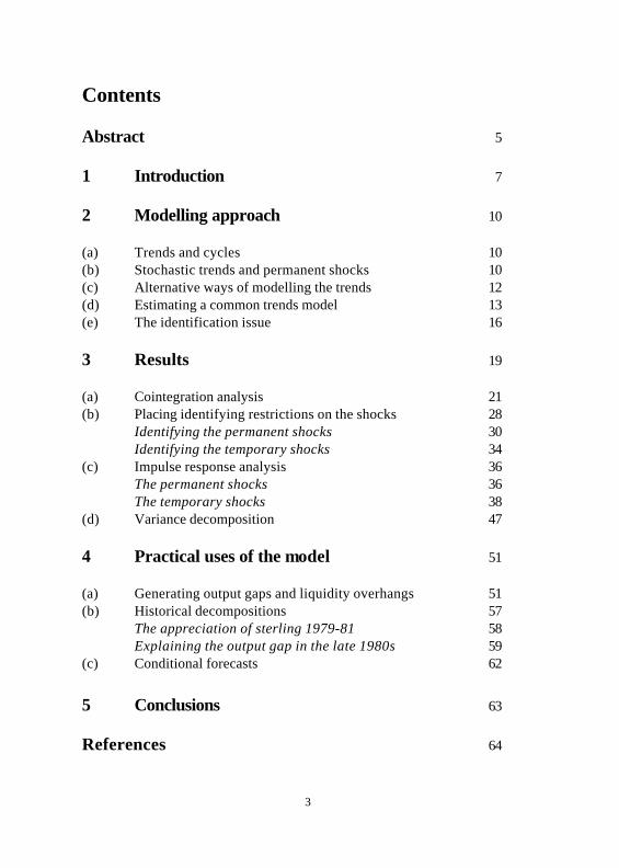
Contents

Abstract 5

1 Introduction 7

2 Modelling approach 10

(a) Trends and cycles 10(b) Stochastic trends and permanent shocks 10(c) Alternative ways of modelling the trends 12(d) Estimating a common trends model 13(e) The identification issue 16

3 Results 19

(a) Cointegration analysis 21(b) Placing identifying restrictions on the shocks 28

Identifying the permanent shocks 30Identifying the temporary shocks 34

(c) Impulse response analysis 36The permanent shocks 36The temporary shocks 38

(d) Variance decomposition 47

4 Practical uses of the model 51

(a) Generating output gaps and liquidity overhangs 51(b) Historical decompositions 57

The appreciation of sterling 1979-81 58Explaining the output gap in the late 1980s 59

(c) Conditional forecasts 62

5 Conclusions 63

References 64

5

Abstract

In this paper we estimate a structural empirical model of the UK monetarytransmission mechanism, which can be used for policy analysis andforecasting. We model a small system of eight variables that theoreticallyhave an important role in the transmission mechanism. The aim is todecompose the movements of each of these variables into a small number ofindependent underlying forcing processes or ‘shocks’, with a well-definedeconomic interpretation. To do this we estimate a statistical (VAR) model ofthe data, on which we impose a minimal number of identifying restrictions.Cointegration analysis is also used to distinguish between permanent shocks,which drive the stochastic trends of the system, and temporary shocks, whichhave purely cyclical effects.

We find that, in addition to identifying shocks to productivity, domesticdemand, external demand and the foreign exchange risk premium, we are ableto distinguish between several types of monetary shock. In particular, we areable to make a distinction between ‘permanent’ monetary policy shocks,attributable to changes in the underlying nominal target of the authorities,and ‘temporary’ policy shocks, reflecting either policy ‘errors’ or transitorydeviations from the authorities’ reaction function. We are also able toidentify a financial intermediation shock, reflecting changes in the provisionof credit by the banking system and the degree of financial liberalisation.

We demonstrate some of the practical uses to which the model can be put.These include: (a) estimating the deviation of each of the variables fromlong-run equilibrium to generate measures of the output gap and the size ofliquidity under/overhangs; (b) analysing the importance of different shocksfor each of the variables over different periods in UK economic history; and(c) generating conditional inflation forecasts based on different paths for thestochastic trends and monetary policy.

7

1 Introduction

In this paper we describe a small, structural empirical model of the UKmonetary transmission mechanism, which can be used for policy analysis andforecasting. As with the companion analytical model project (see Dhar andMillard (2000)), our concern is with the role of money in the transmissionmechanism, and so we focus on the interactions between nominal and realvariables and their relationship with inflation. The model is very much in thespirit of the Bank of England’s ‘pluralist’ approach to modelling andforecasting (see Bank of England (1999)). So even though we aim to developa model in which the monetary channels of influence are spelled out directly,our small stylised model ignores many features of the real world that are ofmajor importance to policy-makers, such as a detailed treatment of the labourmarket. We do this in order to focus on issues that are important to monetaryeconomists.

Our methodological approach to forecasting informs the kind of model wewant to construct. Specifically, we want to generate conditional forecasts,based on relatively few assumptions about economic primitives. Byprimitives we mean fundamental shocks, trends or forcing processes, whichultimately drive the endogenous variables. These fundamentals might includetrend productivity growth, trend velocity growth and the nominal anchor.Our approach to forecasting is as follows: given assumptions about theseprimitives, and given our estimated model of the propagation mechanism,what is the conditional forecast of inflation?

A prerequisite therefore is that the model we use is structural, in the sensethat we can assign economic meaning to the sources of uncertainty in ourmodel.(1) A weakness of the large macro-model approach to forecasting is thatthe complexity and large number of sources of uncertainty in these modelssometimes make it difficult to understand why certain results are generated.The model we develop is small, with eight endogenous variables, and we usetheory-consistent criteria to identify eight economic shocks, of which four

________________________________________________(1) Note that this use of the word ‘structural’ differs slightly from that of the dynamicstochastic general equilibrium (DSGE) school, where the term refers to a model in whichall parameters have economic interpretations in terms of primitives, such as preferencesand technology.

8

have permanent effects on the endogenous variables and four have onlytemporary effects.

The relationship with previous work

We aim to build on previous work on monetary forecasting models. Perhapsthe most influential of these is the ‘P-Star’ model, first applied in a US contextby Hallman, Porter and Small (1991). This model in effect makes the quantitytheory operational by inverting the equation of exchange to relate the trendprice level (p*) to trend velocity (v*) and potential output (y*). The actualprice level is then assumed to adjust to this trend price level, according to anestimated distributed lag process.

Such a model is attractive because it accords the quantity theory a centralrole, but it is clearly non-structural. All the dynamics of the transmissionmechanism are represented in the distributed lag process for prices and, moreoften than not, the estimates of trend velocity and potential output requiredto estimate p* are purely statistical constructs, and hence difficult to interpretas economically meaningful concepts. The approach we adopt in this paper issomewhat different from the basic P-star framework. We expand the numberof variables considered to a set that might be thought of as a minimalrepresentation of the UK transmission mechanism. And then we use moregeneral restrictions derived from economic theory to identify trends invelocity, output, the nominal anchor and other trends in a structural vectorautoregression (VAR) containing all these variables.

We also aim to tie in our model with the work on monetary overhangs(‘M-M*’) previously carried out within the Bank (see Thomas (1997a,b,c)).This work estimated long-run money demand functions for different sectors inthe economy, to produce estimates of monetary under/overhangs or liquiditygaps. While this work proved useful in identifying and calibrating thepotential risks from strong monetary growth, it also showed that the dynamicinteraction between money holdings, activity and prices was likely to dependon the shock that had hit the economy. In this paper we build on the M-M*work, by being able to show explicitly how the relationship between money,activity and prices differs according to which fundamental shock hits theeconomy. We are also able to construct different concepts of the liquiditygap, each of which may have a different link with output and inflation.

9

We also regard this paper as highly complementary to work on analyticalmodels that embody temporary liquidity overhangs, as outlined in Dhar andMillard (2000). That project involves the construction of a dynamicstochastic general equilibrium (DSGE) model of the transmission mechanism,which aims at consolidating our understanding of the role of money. DSGEmodels, when linearised, can usually be written as a first-order vectorautoregression. Consequently, the model developed in this paper can bethought of as the empirical counterpart to the DSGE model developedelsewhere.

The structure of the paper is as follows. In the next section, we describe ouroverall approach to modelling economic time series. It explains how wedecompose the movements of the variables in our system into economicallymeaningful shocks, through placing sufficient restrictions on a statisticalmodel of the data. In Section 3, we set up the system of variables to bemodelled, and apply the techniques of Section 2 to obtain a representation ofthe variables in terms of the permanent and temporary structural shocks. Theproperties of the model are then examined through impulse response andvariance decomposition analysis. Section 4 of the paper gives ademonstration of the practical uses of the model. This includes generatingestimates of the deviation from trend for each variable (eg producingestimates of output gaps and liquidity overhangs); analysing the importanceof different shocks as sources of movement for each of the variables overparticular historical periods (we look at a number of case studies such as theappreciation of sterling 1979-81); and generating conditional forecasts, basedon different assumptions about the future paths of the permanent andtemporary shocks driving the system.

10

2 Modelling approach—how do we model time seriesmovements?

In this section, we describe our general approach to modelling the time serieswe are interested in. In particular, we describe what we mean by the terms‘permanent’ and ‘temporary’ shock and the terms ‘trend’ and ‘cycle’. Wealso explain how we ‘identify’ them, ie give them an economic interpretation.

(a) Trends and cycles

We model our time series as the sum of two components, a trend and a cycle:

ttt vxx )L(F0 Φ++= τ (1)

where

x t = a vector of the n time series of interest at time t.

Fτt = the non-stationary or permanent components of xt , with τt = the trendsand F = loading matrix (ie how each trend affects each of the variables in thelong run).

Φ(L) vt = the stationary or temporary components of xt, with vt a vector ofwhite noise disturbances, which generate dynamic or ‘cyclical’ effectsthrough the distributed lag matrix Φ(L), where L is the lagoperator (Ln vt = vt-n). So Φ(L)vt is a stationary distributed lag ofcurrent and past disturbances = Φ0 vt + Φ1Lvt + Φ2L

2vt ... orequivalently = Φ0 vt + Φ1 vt-1 +...

(b) Stochastic trends and permanent shocks

In addition to the usual deterministic growth or ‘drift’ term, we allow thetrends to have a stochastic or random component, made up of a sequence ofsmall random disturbances. Since these disturbances have a permanent effecton each of the variables, they are termed the ‘permanent shocks’.

11

ttt 11 ητµτ +−+= (2)

or

∑==

−+t

jjttt

01ηµτ (2a)

where µ represents deterministic growth and η1t are the permanent shocks. Soour stochastic trends are simply a vector of random walks with drift. And thestochastic part of the trend is simply the sum of the current and pastpermanent shocks to hit the economy .(2)

Since our trends are stochastic, there is no reason to restrict the permanentshocks driving these trends from having cyclical effects (ie dynamic effectsthat differ from the long-run effects). So the vector vt contains bothpermanent and temporary shocks:

]'[ 21 tttv ηη=

where η2t are purely temporary shocks, which do not have a long-run impacton xt and so do not form part of the stochastic trends.

So in general, our trend-cycle model for xt can be written in terms of thepermanent and temporary shocks as:

∑= Φ+++−

=−

t

tt

iittt xx

2

11

010 )L( F

η

ηηµ (3)

where F is a n x k matrix, where k is the number of permanent shocks drivingthe system. Such a representation is often called a moving-average (‘MA’)representation, as it describes movements in xt as a weighted moving averageof current and past shocks.

________________________________________________(2) When the trends have a stochastic component, xt is said to be a‘difference-stationary’ rather than a ‘trend-stationary’ process.

12

(c) Alternative ways of modelling the trends

There are of course other ways of modelling the non-stationary componentsof our series. One obvious alternative is to model them as simple lineardeterministic trends. In this case, the shocks in the model affect only thecyclical movements of each variable and are independent of the systematicforces driving the trends.

Another way of modelling the trends is as a sequence of one-off deterministicregime shifts:

1* −++= ttt D τµµτ (4)

∑+==

−

t

iittt D

0*µµτ (4a)

where D is a vector of impact dummy variables and ∑=

−

t

iitD

0a vector of

one-zero step-dummies.

In this case, the non-stationarity of xt is the result of a number of largerelatively infrequent ‘regime’ shifts, rather than a sequence of successivesmall random changes.(3) This may be important for some of the trends wewish to identify. For example, the underlying nominal anchor or permanentcomponent of inflation may be best modelled as a series of known shifts inthe policy regime, rather than a sequence of small incremental changes. Asimilar argument may be used for modelling the trend in financialliberalisation.

In this paper, we attempt to model our stochastic trends without the aid ofany deterministic regime shifts.(4) The statistical model we estimate later isrelatively stable over the sample period, suggesting that it is reasonable tomodel the non-stationarity of our variables in terms of random walks withdrift. But this is only weak evidence, and such a choice should not be based________________________________________________(3) The dummy terms can be generalised to allow for shifts in the deterministic growthor drift term.(4) Indeed we do not use any dummies in our system, even those that only generatetemporary movements in the variables.

13

on empirical evidence alone. In future work we intend to compare the resultsbelow with results based on a system where at least some of thenon-stationarity in the system is captured by deterministic regime shifts.

(d) Estimating a common trends model

The estimation of a model such as (1) proceeds by recognising that it is theinverse representation of a VAR model:

tt edxA +=)(L (5)

where A(L) = A0 + A1L + A2L2...

and the structural shocks that we ultimately recover, through the use ofeconomic identifying restrictions, are simply a transformation of the VARresiduals et. For the moment, we leave the identification issue aside andproceed as if the VAR residuals, et, are equivalent to the economic shocks wewish to recover, denoted earlier as ηt. This is to focus attention ondetermining the number of permanent and temporary shocks driving thesystem. This has an important bearing on how we invert the VARrepresentation to yield an MA representation.

The number of permanent shocks depends upon the cointegrating propertiesof the data. Loosely speaking, two or more non-stationary variables are saidto cointegrate if a linear combination of them is found to be stationary. Inother words, the non-stationary or trend components of the variables tend tomove together over time in some proportion, and the linear combination of thevariables can be thought of as defining a long-run equilibrium relationship.This in turn implies that the non-stationary components of these variables aredriven by a ‘common’ stochastic trend (or trends). The implication is thatthere are fewer stochastic trends or permanent shocks than there areendogenous variables. And the number of columns in the matrixF = k < n .

To see the duality between cointegration and the existence of commonstochastic trends, we rewrite the VAR above in vector error-correction(VECM) form, where the long-run relationships between the levels of thevariables in xt are isolated in the matrix Π:

14

ttt exdxB +Π+=∆ −1)L( (6)

If none of the variables cointegrate, then Π = 0, and we are left with astandard VAR in the first differences of the variables

tt edxB +=∆)L( (7)

This, in most cases, can be easily inverted to yield the MA representation:

tt ecx )L(+=∆ µ where 1)L()L( −= Bc (8)

and rewriting in terms of trends and cycles

teCCxxt

iittt e )L(*)1(

1

00 +++= ∑

−

=−µ (9)

where )]1()L([1)L1()L(* CCC −−−= and )1(C is the long-run impact

matrix equivalent to F above. In this case, the matrix F is an n x n matrix, andthere are k = n stochastic trends driving xt.

If the variables are cointegrated with r cointegrating vectors or long-runrelationships in the data, then rank (Π)=r and Π can be written as βα ′Π = ,

where β is an n x r matrix of r cointegrating vectors, and α is an n x r matrix offactor loadings. Inverting the VAR is more difficult in this case. We can stillwrite the model as

teCCxxt

iittt e )L(*

1

00 )1( +∑++=

−

=−µ (10)

But this time, C(1) = F is a reduced rank matrix (rank = n - r), which Engle andGranger (1987) and Engle and Yoo (1991) show can be written as the productof two matrices C(1) = γ θ′. γ and θ are n x n-r (or equivalently n x k) matricesrelated (non-uniquely) to the parameters of the cointegrating vectors α and βthrough the relationships β′ γ = 0 and θ′α = 0. In this case, the trend cycledecomposition of xt should be written:

ttt eCtxx )L(*0 +++= τγµ (11)

15

where there are n-r common stochastic trends (CSTs) given by:

∑θ′−

=−=

1

0

t

iitt eτ (12)

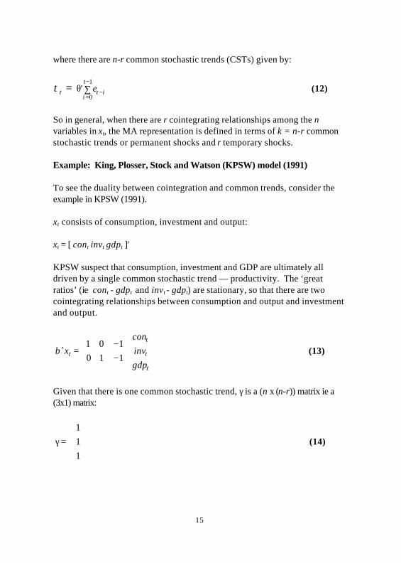
So in general, when there are r cointegrating relationships among the nvariables in xt, the MA representation is defined in terms of k = n-r commonstochastic trends or permanent shocks and r temporary shocks.

Example: King, Plosser, Stock and Watson (KPSW) model (1991)

To see the duality between cointegration and common trends, consider theexample in KPSW (1991).

xt consists of consumption, investment and output:

xt = [ cont invt gdpt ]′

KPSW suspect that consumption, investment and GDP are ultimately alldriven by a single common stochastic trend — productivity. The ‘greatratios’ (ie cont - gdpt and invt - gdpt) are stationary, so that there are twocointegrating relationships between consumption and output and investmentand output.

−−

=′

t

t

t

t

gdpinvcon

x110101

β (13)

Given that there is one common stochastic trend, γ is a (n x (n-r)) matrix ie a(3x1) matrix:

=γ

111

(14)

16

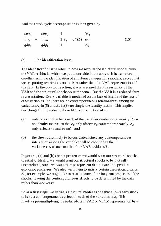
And the trend-cycle decomposition is then given by:

∆+

+

=

t

t

t

t

t

t

t

eeLc

gdpinvcon

gdpinvcon

3

2

0

0

0

)(*111 τ

τ (15)

(e) The identification issue

The identification issue refers to how we recover the structural shocks fromthe VAR residuals, which we put to one side in the above. It has a naturalcorollary with the identification of simultaneous equations models, except thatwe are putting restrictions on the MA rather than the VAR representation ofthe data. In the previous section, it was assumed that the residuals of theVAR and the structural shocks were the same. But the VAR is a reduced-formrepresentation. Every variable is modelled on the lags of itself and the lags ofother variables. So there are no contemporaneous relationships among thevariables: A0 in (5) and B0 in (6) are simply the identity matrix. This impliestwo things for the reduced-form MA representation of xt :

(a) only one shock affects each of the variables contemporaneously (C0 isan identity matrix, so that e1t only affects x1t contemporaneously, e2t

only affects x2t and so on); and

(b) the shocks are likely to be correlated, since any contemporaneousinteraction among the variables will be captured in thevariance-covariance matrix of the VAR residuals Σ.

In general, (a) and (b) are not properties we would want our structural shocksto satisfy. Ideally, we would want our structural shocks to be mutuallyuncorrelated, since we want them to represent distinct and independenteconomic processes. We also want them to satisfy certain theoretical criteria.So, for example, we might like to restrict some of the long-run properties of theshocks, leaving the contemporaneous effects to be determined by the data,rather than vice versa .

So as a first stage, we define a structural model as one that allows each shockto have a contemporaneous effect on each of the variables in xt. Thisinvolves pre-multiplying the reduced-form VAR or VECM representation by a

17

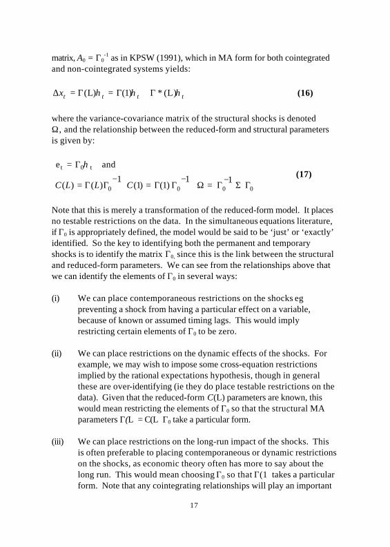
matrix, A0 = Γ0-1 as in KPSW (1991), which in MA form for both cointegrated

and non-cointegrated systems yields:

ttttx ηηη )L(*)1()L( Γ+Γ=Γ=∆ (16)

where the variance-covariance matrix of the structural shocks is denotedΩ, and the relationship between the reduced-form and structural parametersis given by:

0000

t0t

11)1()1(

1)()(

and=e

ΓΣ−Γ=Ω−

ΓΓ=−

ΓΓ=

Γ

CLLC

η (17)

Note that this is merely a transformation of the reduced-form model. It placesno testable restrictions on the data. In the simultaneous equations literature,if Γ0 is appropriately defined, the model would be said to be ‘just’ or ‘exactly’identified. So the key to identifying both the permanent and temporaryshocks is to identify the matrix Γ0, since this is the link between the structuraland reduced-form parameters. We can see from the relationships above thatwe can identify the elements of Γ0 in several ways:

(i) We can place contemporaneous restrictions on the shocks egpreventing a shock from having a particular effect on a variable,because of known or assumed timing lags. This would implyrestricting certain elements of Γ0 to be zero.

(ii) We can place restrictions on the dynamic effects of the shocks. Forexample, we may wish to impose some cross-equation restrictionsimplied by the rational expectations hypothesis, though in generalthese are over-identifying (ie they do place testable restrictions on thedata). Given that the reduced-form C(L) parameters are known, thiswould mean restricting the elements of Γ0 so that the structural MAparameters Γ(L) = C(L) Γ0 take a particular form.

(iii) We can place restrictions on the long-run impact of the shocks. Thisis often preferable to placing contemporaneous or dynamic restrictionson the shocks, as economic theory often has more to say about thelong run. This would mean choosing Γ0 so that Γ(1) takes a particularform. Note that any cointegrating relationships will play an important

18

part in this, since the matrix of long-run multipliers is of reduced rankand can be split into Γ(1) = [F 0] satisfying β ′F = 0 (see KPSW (1991)and Wickens (1996)).

(iv) Finally, we can place restrictions such that the variance-covariancematrix of the structural shocks takes a particular form. As arguedearlier, we would want our structural shocks to be orthogonal to oneanother, and so we might want to place the restrictions that

Γ0−1 Σ Γ0 = Ω = I.

In this paper, we use a combination of restrictions (iii) and (iv) to identify thepermanent shocks, and (i) and (iv) to identify the temporary shocks. In thepresence of cointegrating relationships, KPSW (1991) and Warne (1991) showthat Γ0 can be partitioned into two matrices = [H J], which allows us to breakdown the identification of Γ0 into several stages:

(i) Cointegrating restrictions that determine the rank of H and J, and placesome restrictions on the pattern of H. These impose (n-r) x rrestrictions on Γ0.

(ii) Identifying the permanent shocks. This involves orthogonalityrestrictions on the permanent shocks, as well as long-run restrictions.This provides (n-r)2 restrictions (see Mellander et al (1992)).

(iii) Orthogonality between the permanent and temporary shocks. Thisimposes r(n-r) restrictions.

(iv) Identifying the transitory shocks using orthogonality andcontemporaneous restrictions. This provides r2 additional restrictions.

In all, we impose n2 restrictions on Γ0, which is the minimum we need toidentify exactly its n2 elements. Following KPSW (1991), we also place sometestable over-identifying restrictions on the cointegrating vectors at stage (i).This is to ensure that our cointegrating vectors represent, as far as possible,sensible long-run equilibrium relationships. As we will see, this is useful intying down some of the long-run multipliers.

19

3 Results

To estimate our structural monetary model, we consider a system of eightvariables, all of which are thought to play a significant role in the monetarytransmission mechanism of the UK economy.

• m - p : real M4 (break-adjusted nominal M4, deflated by the GDP market-price deflator)

• y : real GDP at market prices• is : base rate• il : long-term interest rates• pk : real asset prices (FTSE All-Share index deflated by the

GDP market-price deflator)• ∆p : Three-month annualised rate of seasonally adjusted

RPIX inflation• id : the weighted own-rate on M4 (a weighted average of

bank and building society deposit rates)• e : The real effective exchange rate (the nominal effective

rate multiplied by relative unit labour costs; a rise in erepresents a real appreciation).

The first six variables are fairly representative of those used in typicalclosed-economy monetary models of the transmission mechanism, see eg themodel of Blanchard (1981), which examines the links between money, assetprices, bond yields and inflation in a rational-expectations framework. Weaugment these variables with the own-rate on M4 and the real exchange rate.This allows us to extend the basic closed monetary economy model to thecase of a small open economy with a banking system.(5) Developments in theUK economy’s relationship with overseas economies (eg changes inexchange rate regimes and trading relationships such as the common market)and changes in the structure and competitiveness of the banking system (egthe financial controls of the 1970s and the liberalisation of the 1980s) havebeen important influences on the UK economy over the past thirty years. Soany empirical monetary model needs to encompass them. But this potentially

________________________________________________(5) See Dornbusch (1976) and Obstfeld and Rogoff (1996) for examples of smallopen-economy models, and Fischer (1983) and Dhar and Millard (2000) for models thatincorporate a banking system.

20

adds to the number of stochastic trends driving the system, eg overseasdemand and banking sector shocks.

Data for these variables exists over the period 1964 Q1 to 1998 Q2, which weuse as our sample period. It is true that this sample period encompasses anumber of potential regime shifts, such as the movement from fixed to floatingexchange rates in 1972 and 1992. As discussed earlier, we attempt to modelsuch changes as part of the stochastic trends (ie as one of a series ofsuccessive permanent shocks), rather than as large one-off events throughthe use of deterministic shift dummies. Tests of the stability of the estimatedsystem give an idea of how reasonable this assumption is. But we intend toexperiment with different ways of allowing for regime shifts in future work.

The estimation and analysis of our structural empirical model is carried out inseveral stages:

• Cointegration analysis. The unrestricted VAR system containing thelevels of all the variables is estimated, and Johansen’s (1988) MLprocedure for determining the cointegrating rank of the system is applied.This is to determine the number of common stochastic trends in thesystem. We also place some (over)identifying restrictions on thecointegrating vectors as a first stage in identifying the shocks, althoughas argued by Warne (1991), this is not a necessity to identify a SVARmodel.

• Placing structural identifying restrictions on the shocks to obtain anSVAR model. The reduced-form errors of the VECM system aretransformed into structural shocks, using identifying restrictions on theshort and long-run impact of the shocks as discussed earlier.

• Impulse response analysis. The dynamic impact of the identified shockson each of the variables is analysed to see if the predictions are sensible.

• Variance decomposition. The importance of each of the permanentshocks in driving each variable in the system is examined, at differenttime horizons.

It is important to emphasise that the identifying restrictions we impose are notmeant to be set in stone, especially as some of them are controversial andmodel-dependent. They are meant to illustrate what sort of restrictions can be

21

imposed in this framework. In general, we can estimate the structural modelusing a variety of different identifying assumptions, and examine whatdifference it makes to the pattern of the structural shocks and their impact oneach of the variables in the system.

(a) Cointegration analysis

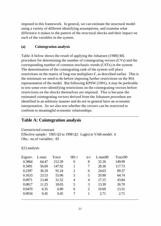
Table A below shows the result of applying the Johansen (1988) MLprocedure for determining the number of cointegrating vectors (CVs) and thecorresponding number of common stochastic trends (CSTs) in the system.The determination of the cointegrating rank of the system will placerestrictions on the matrix of long-run multipliers F, as described earlier. This isthe minimum we need to do before imposing further restrictions on the MArepresentation of the model. But following KPSW (1991), it may be preferableto test some over-identifying restrictions on the cointegrating vectors beforerestrictions on the shocks themselves are imposed. This is because theestimated cointegrating vectors derived from the Johansen procedure areidentified in an arbitrary manner and do not in general have an economicinterpretation. So we also test whether the vectors can be restricted toconform to meaningful economic relationships.___________________________________________________________Table A: Cointegration analysis

Unrestricted constantEffective sample: 1965 Q3 to 1998 Q2: Lag(s) in VAR-model: 6Obs.- no.of variables: 83

I(1) analysis

Eigenv. L-max Trace H0: r n-r L-max90 Trace900.3864 64.47 212.39 0 8 32.26 149.990.3491 56.69 147.92 1 7 28.36 117.730.2397 36.18 91.24 2 6 24.63 89.370.1633 23.53 55.06 3 5 20.90 64.740.0971 13.48 31.52 4 4 17.15 43.840.0817 11.25 18.05 5 3 13.39 26.700.0470 6.35 6.80 6 2 10.60 13.310.0034 0.45 0.45 7 1 2.71 2.71

___________________________________________________________

22

The test results indicate that there are probably four cointegrating vectors atthe 10% significance level. This implies that there are four common stochastictrends driving the eight variables. Blanchard’s (1981) closed-economy modelhas four central equilibrium relationships: a term-structure relationship, anasset pricing equation, a money demand equation and an aggregate demandrelationship. This would suggest four cointegrating relationships: the spreadbetween short rates and long rates (as the expectations hypothesis of theterm structure suggests that short and long rates should be equal in the longrun); an asset price relationship linking real asset prices homogeneously withincome and negatively with real interest rates; a money-demand relationshiplinking real money with income, real asset prices (as a proxy for real wealth),and the opportunity cost of holding money; and an aggregate demandrelationship linking GDP to wealth, interest rates and the exchange rate.

Table B below shows the results of restrictions tests on the CVs that examinewhether they conform to the equilibrium relationships implied by theBlanchard model. At least four restrictions in each equation are needed toidentify the vectors (see Johansen and Juselius (1994), Pesaran and Shin(1995)). The initial restrictions we imposed were as follows:

(i) The first vector was restricted to form a money-demand relationship.This involved imposing zero restrictions on all variables except money,GDP and asset prices, and restricting the deposit rate and base rate toform a term in the opportunity cost of holding money (id-is).

(ii) The second vector was restricted to form a term-structure relationship.So the coefficients on short and long rates were restricted to be equalwith opposite sign, and all other coefficients were restricted to be zero.

(iii) The third vector was restricted to be an asset-price relationship. Sothe coefficients on income and asset prices were restricted to be equalin magnitude with opposite sign, as were the coefficients on theshort-term interest rate and inflation. All other coefficients wererestricted to be zero.

(iv) The fourth vector was restricted to be an aggregate demandrelationship. For this we excluded real broad money (no wealth effectas it largely represents inside money) and restricted two of the threeinterest rate coefficients to be zero, leaving the other interest rate to

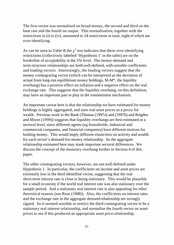
23

take up the burden of affecting aggregate demand. The results werebroadly the same whichever two interest rates were excluded (partlyowing to the restrictions already imposed on the short and long ratesin (ii)).

__________________________________________________

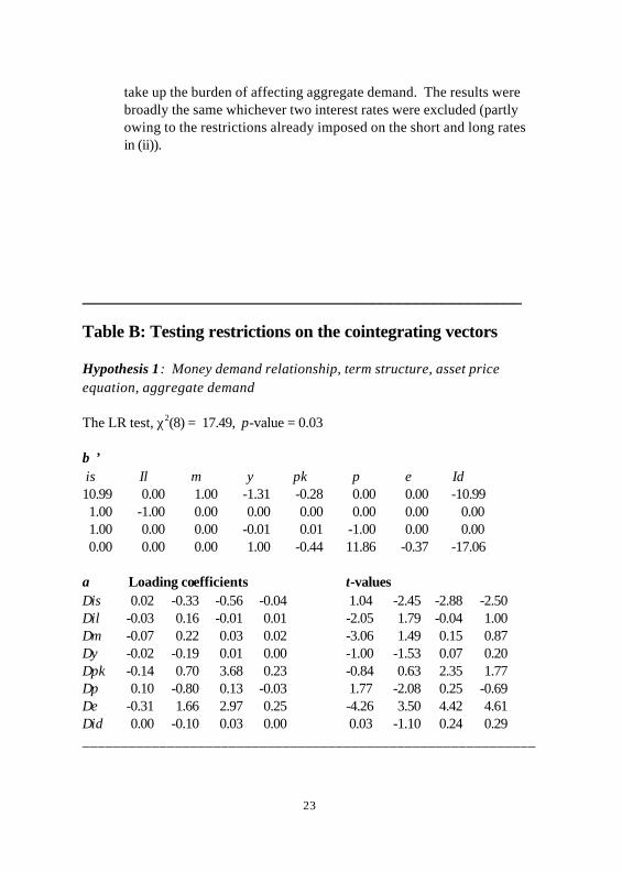
Table B: Testing restrictions on the cointegrating vectors

Hypothesis 1: Money demand relationship, term structure, asset priceequation, aggregate demand

The LR test, χ2(8) = 17.49, p-value = 0.03

β ’is Il m y pk π e Id10.99 0.00 1.00 -1.31 -0.28 0.00 0.00 -10.991.00 -1.00 0.00 0.00 0.00 0.00 0.00 0.001.00 0.00 0.00 -0.01 0.01 -1.00 0.00 0.000.00 0.00 0.00 1.00 -0.44 11.86 -0.37 -17.06

α Loading coefficients t-values∆is 0.02 -0.33 -0.56 -0.04 1.04 -2.45 -2.88 -2.50∆il -0.03 0.16 -0.01 0.01 -2.05 1.79 -0.04 1.00∆m -0.07 0.22 0.03 0.02 -3.06 1.49 0.15 0.87∆y -0.02 -0.19 0.01 0.00 -1.00 -1.53 0.07 0.20∆pk -0.14 0.70 3.68 0.23 -0.84 0.63 2.35 1.77∆π 0.10 -0.80 0.13 -0.03 1.77 -2.08 0.25 -0.69∆e -0.31 1.66 2.97 0.25 -4.26 3.50 4.42 4.61∆id 0.00 -0.10 0.03 0.00 0.03 -1.10 0.24 0.29___________________________________________________________

24

___________________________________________________________

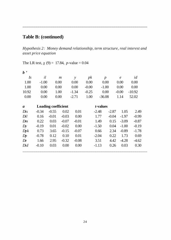
Table B: (continued)

Hypothesis 2: Money demand relationship, term structure, real interest andasset price equation

The LR test, χ (9) = 17.84, p-value = 0.04

β ’Is il m y pk π e id

1.00 -1.00 0.00 0.00 0.00 0.00 0.00 0.001.00 0.00 0.00 0.00 -0.00 -1.00 0.00 0.00

10.92 0.00 1.00 -1.34 -0.25 0.00 -0.00 -10.920.00 0.00 0.00 -2.71 1.00 -36.08 1.14 52.02

α Loading coefficient t-values∆is -0.34 -0.55 0.02 0.01 -2.48 -2.87 1.05 2.49∆il 0.16 -0.01 -0.03 0.00 1.77 -0.04 -1.97 -0.99∆m 0.22 0.03 -0.07 -0.01 1.49 0.15 -3.09 -0.87∆y -0.19 0.01 -0.02 0.00 -1.50 0.04 -1.00 -0.19∆pk 0.73 3.65 -0.15 -0.07 0.66 2.34 -0.89 -1.78∆p -0.78 0.12 0.10 0.01 -2.04 0.22 1.73 0.69∆e 1.66 2.95 -0.32 -0.08 3.51 4.42 -4.28 -4.62∆id -0.10 0.03 0.00 0.00 -1.13 0.26 0.03 0.30___________________________________________________________

25

The first vector was normalised on broad money, the second and third on thebase rate and the fourth on output. This normalisation, together with therestrictions in (i) to (iv), amounted to 24 restrictions in total, eight of which areover-identifying.

As can be seen in Table B the χ2 test indicates that these over-identifyingrestrictions (collectively labelled ‘Hypothesis 1’ in the table) are on theborderline of acceptability at the 5% level. The money-demand andterm-structure relationships are both well-defined, with sensible coefficientsand loading vectors. Interestingly, the loading vectors suggest that themoney cointegrating vector (which can be interpreted as the deviation ofactual from long-run equilibrium money holdings, M-M*, the liquidityoverhang) has a positive effect on inflation and a negative effect on the realexchange rate. This suggests that the liquidity overhang, on this definition,may have an important part to play in the transmission mechanism.

An important caveat here is that the relationship we have estimated for moneyholdings is highly aggregated, and uses real asset prices as a proxy forwealth. Previous work in the Bank (Thomas (1997a) and (1997b) and Brigdenand Mizen (1999)) suggests that liquidity overhangs are best estimated at asectoral level, since different agents (eg households, industrial andcommercial companies, and financial companies) have different motives forholding money. This would imply different elasticities on activity and wealthfor each sector’s demand-for-money relationship. So the aggregaterelationship estimated here may mask important sectoral differences. Wediscuss the concept of the monetary overhang further in Section 4 of thispaper.

The other cointegrating vectors, however, are not well-defined underHypothesis 1. In particular, the coefficients on income and asset prices areextremely low in the third identified vector, suggesting that the realshort-term interest rate is close to being stationary. This would be plausiblefor a small economy if the world real interest rate was also stationary over thesample period. And a stationary real interest rate is also appealing for othertheoretical reasons (see Rose (1988)). Also, the coefficients on interest ratesand the exchange rate in the aggregate demand relationship are wronglysigned. So it seemed sensible to restrict the third cointegrating vector to be astationary real interest relationship, and normalise the fourth vector on assetprices to see if this produced an appropriate asset price relationship.

26

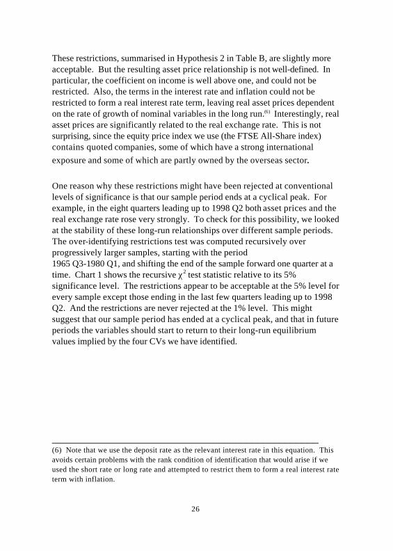
These restrictions, summarised in Hypothesis 2 in Table B, are slightly moreacceptable. But the resulting asset price relationship is not well-defined. Inparticular, the coefficient on income is well above one, and could not berestricted. Also, the terms in the interest rate and inflation could not berestricted to form a real interest rate term, leaving real asset prices dependenton the rate of growth of nominal variables in the long run.(6) Interestingly, realasset prices are significantly related to the real exchange rate. This is notsurprising, since the equity price index we use (the FTSE All-Share index)contains quoted companies, some of which have a strong internationalexposure and some of which are partly owned by the overseas sector.

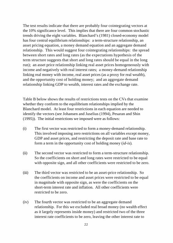
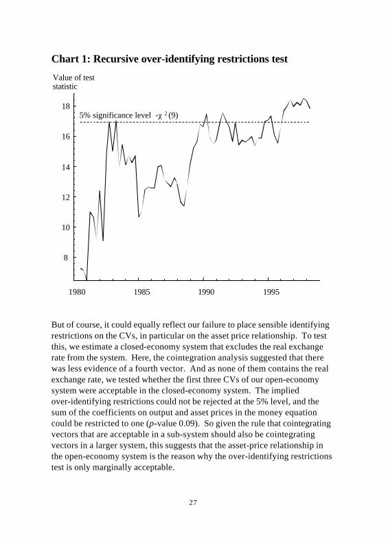
One reason why these restrictions might have been rejected at conventionallevels of significance is that our sample period ends at a cyclical peak. Forexample, in the eight quarters leading up to 1998 Q2 both asset prices and thereal exchange rate rose very strongly. To check for this possibility, we lookedat the stability of these long-run relationships over different sample periods.The over-identifying restrictions test was computed recursively overprogressively larger samples, starting with the period1965 Q3-1980 Q1, and shifting the end of the sample forward one quarter at atime. Chart 1 shows the recursive χ2 test statistic relative to its 5%significance level. The restrictions appear to be acceptable at the 5% level forevery sample except those ending in the last few quarters leading up to 1998Q2. And the restrictions are never rejected at the 1% level. This mightsuggest that our sample period has ended at a cyclical peak, and that in futureperiods the variables should start to return to their long-run equilibriumvalues implied by the four CVs we have identified.

________________________________________________(6) Note that we use the deposit rate as the relevant interest rate in this equation. Thisavoids certain problems with the rank condition of identification that would arise if weused the short rate or long rate and attempted to restrict them to form a real interest rateterm with inflation.

27

Chart 1: Recursive over-identifying restrictions test

But of course, it could equally reflect our failure to place sensible identifyingrestrictions on the CVs, in particular on the asset price relationship. To testthis, we estimate a closed-economy system that excludes the real exchangerate from the system. Here, the cointegration analysis suggested that therewas less evidence of a fourth vector. And as none of them contains the realexchange rate, we tested whether the first three CVs of our open-economysystem were acceptable in the closed-economy system. The impliedover-identifying restrictions could not be rejected at the 5% level, and thesum of the coefficients on output and asset prices in the money equationcould be restricted to one (p-value 0.09). So given the rule that cointegratingvectors that are acceptable in a sub-system should also be cointegratingvectors in a larger system, this suggests that the asset-price relationship inthe open-economy system is the reason why the over-identifying restrictionstest is only marginally acceptable.

1980 1985 1990 1995

8

10

12

14

16

185% significance level -χ 2 (9)

Value of teststatistic

28

Given their broad acceptability over time and in smaller sub-systems (and alsoremembering that we have not added any dummy variables to our system), wetake the CVs we have identified as reasonably acceptable long-runrelationships. But in our subsequent analysis, we point out where the assetprice relationship might be having an impact on the results.

(b) Placing identifying restrictions on the shocks

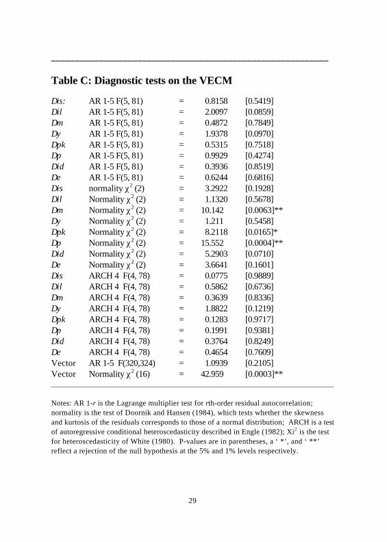
Following the cointegration analysis, the next stage is to estimate the VECMrepresentation (equation (6) above) with the cointegrating rank and therestrictions on the CVs imposed. Despite having some doubts about theidentification of the cointegrating vectors in Section (a), the estimated VECMhas reasonably good statistical properties. Table C below shows somediagnostic tests on the VECM. The only major statistical problems are withthe normality of the residuals of the inflation and real money equations. Aninspection of the residuals shows that this is largely related to the large hikein VAT in 1979 Q3, which had the temporary effect, over one quarter, ofraising inflation and reducing real balances. An appropriate dummy variablefor this period is a possible solution. But for now we stick to our initialstrategy, which is to attempt to model our system of variables without the aidof any deterministic variables. So this VAT effect will be captured in one ofour identified shocks.

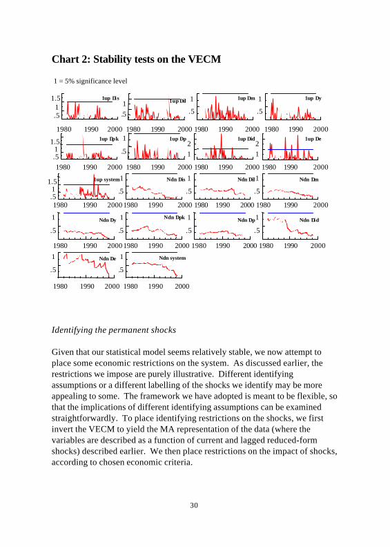
The VECM also seems to be a reasonably stable statistical model. Chart 2shows recursive one-step (labelled 1up) and break-point (labelled Ndn) Chowtest statistics for each equation in the system (relative to their 5% significancelevel), as well as a test for the system as a whole. None of the equationsappears to show any major sign of a structural break (except perhaps,unsurprisingly, the real exchange rate over the ERM period), which impliesthat our attempt to capture the non-stationarity in our system via thestochastic trends is not entirely unreasonable.

29

__________________________________________________________

Table C: Diagnostic tests on the VECM

∆is: AR 1-5 F(5, 81) = 0.8158 [0.5419]∆il AR 1-5 F(5, 81) = 2.0097 [0.0859]∆m AR 1-5 F(5, 81) = 0.4872 [0.7849]∆y AR 1-5 F(5, 81) = 1.9378 [0.0970]∆pk AR 1-5 F(5, 81) = 0.5315 [0.7518]∆π AR 1-5 F(5, 81) = 0.9929 [0.4274]∆id AR 1-5 F(5, 81) = 0.3936 [0.8519]∆e AR 1-5 F(5, 81) = 0.6244 [0.6816]∆is normality χ2 (2) = 3.2922 [0.1928]∆il Normality χ2 (2) = 1.1320 [0.5678]∆m Normality χ2 (2) = 10.142 [0.0063]**∆y Normality χ2 (2) = 1.211 [0.5458]∆pk Normality χ2 (2) = 8.2118 [0.0165]*∆π Normality χ2 (2) = 15.552 [0.0004]**∆id Normality χ2 (2) = 5.2903 [0.0710]∆e Normality χ2 (2) = 3.6641 [0.1601]∆is ARCH 4 F(4, 78) = 0.0775 [0.9889]∆il ARCH 4 F(4, 78) = 0.5862 [0.6736]∆m ARCH 4 F(4, 78) = 0.3639 [0.8336]∆y ARCH 4 F(4, 78) = 1.8822 [0.1219]∆pk ARCH 4 F(4, 78) = 0.1283 [0.9717]∆π ARCH 4 F(4, 78) = 0.1991 [0.9381]∆id ARCH 4 F(4, 78) = 0.3764 [0.8249]∆e ARCH 4 F(4, 78) = 0.4654 [0.7609]Vector AR 1-5 F(320,324) = 1.0939 [0.2105]Vector Normality χ2 (16) = 42.959 [0.0003]**_____________________________________________________________________

Notes: AR 1-r is the Lagrange multiplier test for rth-order residual autocorrelation;normality is the test of Doornik and Hansen (1984), which tests whether the skewnessand kurtosis of the residuals corresponds to those of a normal distribution; ARCH is a testof autoregressive conditional heteroscedasticity described in Engle (1982); Xi2 is the testfor heteroscedasticity of White (1980). P-values are in parentheses, a ‘ *’, and ‘ **’reflect a rejection of the null hypothesis at the 5% and 1% levels respectively.

30

Chart 2: Stability tests on the VECM

Identifying the permanent shocks

Given that our statistical model seems relatively stable, we now attempt toplace some economic restrictions on the system. As discussed earlier, therestrictions we impose are purely illustrative. Different identifyingassumptions or a different labelling of the shocks we identify may be moreappealing to some. The framework we have adopted is meant to be flexible, sothat the implications of different identifying assumptions can be examinedstraightforwardly. To place identifying restrictions on the shocks, we firstinvert the VECM to yield the MA representation of the data (where thevariables are described as a function of current and lagged reduced-formshocks) described earlier. We then place restrictions on the impact of shocks,according to chosen economic criteria.

1980 1990 2000

.51

1.5 1up ∆i s

1980 1990 2000

.51 1up ∆il

1980 1990 2000

.5

1 1up ∆m

1980 1990 2000

.5

1 1up ∆y

1980 1990 2000.51

1.5 1up ∆pk

1980 1990 2000

.5

1 1up ∆π

1980 1990 2000

12

1up ∆id

1980 1990 2000

12

1up ∆e

1980 1990 2000.51

1.5 1up system

1980 1990 2000

.5

1 Ndn ∆is

1980 1990 2000

.5

1 Ndn ∆il

1980 1990 2000

.5

1 Ndn ∆m

1980 1990 2000

.5

1 Ndn ∆y

1980 1990 2000

.5

1 Ndn ∆pk

1980 1990 2000

.5

1 Ndn ∆π

1980 1990 2000

.5

1 Ndn ∆id

1980 1990 2000

.5

1 Ndn ∆e

1980 1990 2000

.5

1 Ndn system

1 = 5% significance level

31

As discussed in Section 2, we need to place (n-r)2 restrictions to identify thepermanent shocks. Ten of the restrictions can be obtained by assuming thatthe structural permanent shocks are mutually uncorrelated (ie originate fromindependent sources) and have a normalised variance of 1. This leaves sixfurther restrictions to be imposed. As discussed earlier, we impose long-runrestrictions on the impact of the CSTs based on the predictions of theory.

So what type of permanent shocks should we be looking for, and how do weidentify them? Some guidance on this is offered by the cointegration analysiswe carried out earlier. Indeed, it is important that the restrictions we imposeare consistent with the cointegrating vectors we identify. The fact that wehave found cointegrating relationships for money demand, the term structure,real interest rates and asset prices suggests that we should rule outidentifying our permanent shocks as those to money demand, the term andequity risk premia, or the world real interest rate. Consider the term-structurerelationship. The cointegrating vector implies that short and long rates movetogether in the long run. In contrast, the existence of a permanentterm-premium shock (and hence the existence of a term-premium stochastictrend) would imply that short and long rates moved apart over time. So thetwo are inconsistent. A similar argument applies to the other relationships.

This leaves us with several potential candidates for the four fundamentalpermanent shocks:

(1) Domestic productivity/aggregate supply shocks.

(2) Domestic demand shocks, such as shifts in fiscal policy and consumerpreferences.

(3) A permanent nominal shock, reflecting the implicit inflation/moneygrowth target of the authorities. In the absence of full credibility, thismight be interpreted as the trend in inflation expectations or ‘core’inflation.(7)

________________________________________________(7)

There are obvious Lucas critique issues here since a shift in the nominal target of theauthorities might influence the process which agents use to generate their expectations.This would invalidate the assumption of constant parameters in the structural MArepresentation of the system.

32

(4) A financial liberalisation/credit market shock, which affects thecompetitiveness/willingness to lend of the banking system and leads to apermanent shift in the velocity of circulation. Another way to think ofthis is as a shock to the demand and supply of the intermediationservices provided by banks.

(5) Shifts in the pattern of foreign demand and supply, which affect theequilibrium current account.

Given that the real interest rate is stationary, we choose not to identify theaggregate demand shock as one of our permanent shocks. So we assume thatshifts in aggregate demand have no long-run effects on any of the variablesof our system. This is controversial, since in certain open-economy models ashift in aggregate demand will affect the equilibrium real exchange rate in thelong run. The typical mechanism is that, for a given level of equilibriumoutput in the long run, a rise in real domestic demand must be offset by a fallin net external demand, which is engineered through a rise in the realexchange rate.

But this argument only considers the internal balance of the economy, andignores the fact that a current account deficit will result from a shift betweendomestic and overseas demand. The resulting fall in net external assets willcontinue to have negative wealth effects on domestic demand, as long as thedeficit persists. Provided that the propensity to consume out of wealth isgreater than the real rate of return on overseas assets and that the economy issmall relative to the rest of the world, the current account will return tobalance at the initial level of the real exchange rate.(8) So in the long run, stockand flow equilibrium implies that a shift in any of the components of domesticdemand will be offset by a wealth-induced fall in domestic consumption,rather than an exchange rate-induced fall in overseas demand. And as thisdoes not affect the equilibrium level of output or the equilibrium currentaccount, it should have no effect on the real exchange rate.

________________________________________________(8) If the propensity to consume out of wealth is lower than the real interest rate, themodel can become unstable, since the decumulation of assets/accumulation of debt willworsen the debt-service component of the current account faster than it improves thetrade balance component.

33

So we identify the four permanent shocks on the following basis:

• The first shock is identified as a productivity shock (labelled an ASshock) and is restricted to have no long-run impact on the rate ofinflation, although it may have cumulative effects on the price level. Thisshock is also intended to cover shocks to productivity from overseassuch as oil shocks, and shocks emerging from the labour market.

• The second shock we identify as a shock to financial intermediation(labelled FIN). This is left unrestricted, as it is a shock for which we havefew theoretical priors regarding its long-run effects. Potentially, a shift inthe supply of credit could affect long-run output via ‘credit-channel’effects on investment. And we would want such a shock to have asignificant long-run effect on the opportunity cost of holding money; egthe spread between deposit rates and base rates would be expected tonarrow as a result of a financial liberalisation.

• The third shock is identified as a nominal shock (NOM) and is restrictedto have no impact on real output or the real exchange rate in the long run.We allow it to have an effect on real balances and real asset prices, giventhat a rise in core inflation is likely to affect the opportunity cost ofholding M4 (since a small proportion of M4 is non interest bearing) andgiven that one of our cointegrating vectors suggested that the growth ofnominal variables affects real asset prices in the long run.(9)

• The fourth shock is identified as a relative foreign demand (FOR) shockthat permanently affects the equilibrium real exchange rate. It isrestricted to have no long-run impact on output, inflation or any of thedomestic interest rates (this only involves three restrictions, since thestationarity of the real interest rate and the term structure implies thatanything that has a zero long-run effect on inflation also has a zero effecton the short and long-term interest rates). The first of these restrictionsis somewhat controversial, as it implies that even though the realexchange rate changes in the long run, this has no long-run effect on theequilibrium level of output. Thus, we are assuming that in the long run

________________________________________________(9) If we did restrict the inflation rate to have no effect on asset prices, then thenominal shock would have to affect one or more of the other variables in the asset -pricecointegrating vector to ensure consistency.

34

there are no wedge effects that drive a permanent gap between realproduct and consumption wages and that would in turn shift the NAIRU.

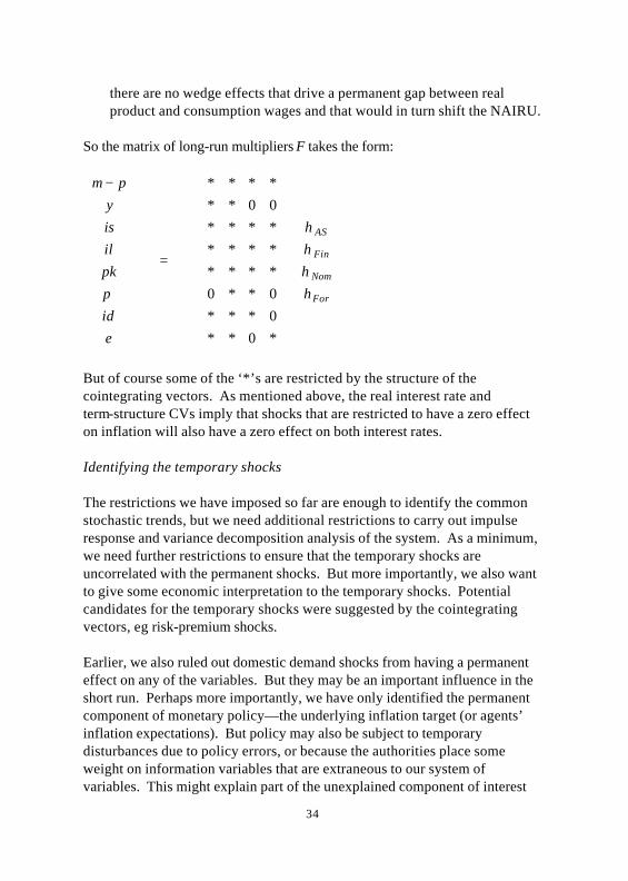
So the matrix of long-run multipliers F takes the form:

=

−

For

Nom

Fin

AS

eid

pkilisy

pm

ηηηη

π

*0**0***0**0************00******

But of course some of the ‘*’s are restricted by the structure of thecointegrating vectors. As mentioned above, the real interest rate andterm-structure CVs imply that shocks that are restricted to have a zero effecton inflation will also have a zero effect on both interest rates.

Identifying the temporary shocks

The restrictions we have imposed so far are enough to identify the commonstochastic trends, but we need additional restrictions to carry out impulseresponse and variance decomposition analysis of the system. As a minimum,we need further restrictions to ensure that the temporary shocks areuncorrelated with the permanent shocks. But more importantly, we also wantto give some economic interpretation to the temporary shocks. Potentialcandidates for the temporary shocks were suggested by the cointegratingvectors, eg risk-premium shocks.

Earlier, we also ruled out domestic demand shocks from having a permanenteffect on any of the variables. But they may be an important influence in theshort run. Perhaps more importantly, we have only identified the permanentcomponent of monetary policy—the underlying inflation target (or agents’inflation expectations). But policy may also be subject to temporarydisturbances due to policy errors, or because the authorities place someweight on information variables that are extraneous to our system ofvariables. This might explain part of the unexplained component of interest

35

rate movements. To see how the permanent and temporary policy shocksinteract, imagine that the authorities on average operate a Taylor rule:

ist = r* + π*t + a (π t - π*t) + (1- a) ( yt - y*t) + ηtpol

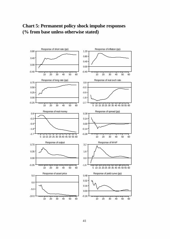
π*t = π*t-1 + ηNom

The temporary policy shock ηtpol then represents any movement in interestrates that deviates from this rule. The permanent policy shock, as discussedearlier, permanently changes π∗, which changes ist one for one in the long run(keeping the real interest rate unchanged at r*), but less than one-for-one inthe short run.

To identify the temporary shocks, we impose contemporaneous restrictions.In addition to the ten restrictions required for orthogonality, we must place sixadditional restrictions on the temporary disturbances to identify them.Unfortunately, these contemporaneous restrictions require us to makeassumptions about the timing relationships between the variables. Inparticular, we are forced to take a stand on such issues as the degree ofnominal rigidity in response to different shocks. The four shocks we attemptto identify and the restrictions we impose are as follows:

(i) A temporary monetary policy shock (labelled TPOL). On the basis ofthere being a lag between interest rate movements and demand, and afurther lag (because of nominal rigidities) between demand andinflation, this shock is restricted to have no contemporaneous impacton output or inflation.

(ii) A domestic demand (AD) shock. This is allowed to have acontemporaneous effect on output, as it is not subject to the first lagmentioned in (i), but no contemporaneous effect on inflation, as it issubject to the second lag.

(iii) A foreign exchange risk-premium shock (FRP). This we interpret as ageneral shift in preferences towards sterling-denominated assets.Again we appeal to timing lags, and this shock is restricted to have noinitial effect on output, prices and additionally the deposit rate,reflecting the stickiness of bank deposit-rate setting, although this lastrestriction is rather arbitrary.

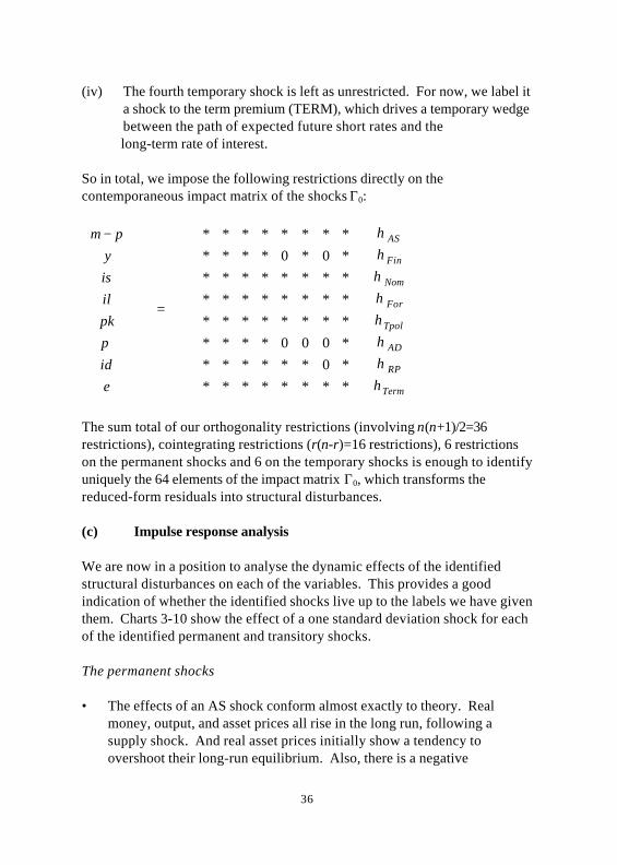
36

(iv) The fourth temporary shock is left as unrestricted. For now, we label ita shock to the term premium (TERM), which drives a temporary wedgebetween the path of expected future short rates and the

long-term rate of interest.

So in total, we impose the following restrictions directly on thecontemporaneous impact matrix of the shocks Γ0:

=

−

Term

RP

AD

Tpol

For

Nom

Fin

AS

eid

pkilisy

pm

ηηηηηηηη

π

*********0*******000*****************************0*0************

The sum total of our orthogonality restrictions (involving n(n+1)/2=36restrictions), cointegrating restrictions (r(n-r)=16 restrictions), 6 restrictionson the permanent shocks and 6 on the temporary shocks is enough to identifyuniquely the 64 elements of the impact matrix Γ0, which transforms thereduced-form residuals into structural disturbances.

(c) Impulse response analysis

We are now in a position to analyse the dynamic effects of the identifiedstructural disturbances on each of the variables. This provides a goodindication of whether the identified shocks live up to the labels we have giventhem. Charts 3-10 show the effect of a one standard deviation shock for eachof the identified permanent and transitory shocks.

The permanent shocks

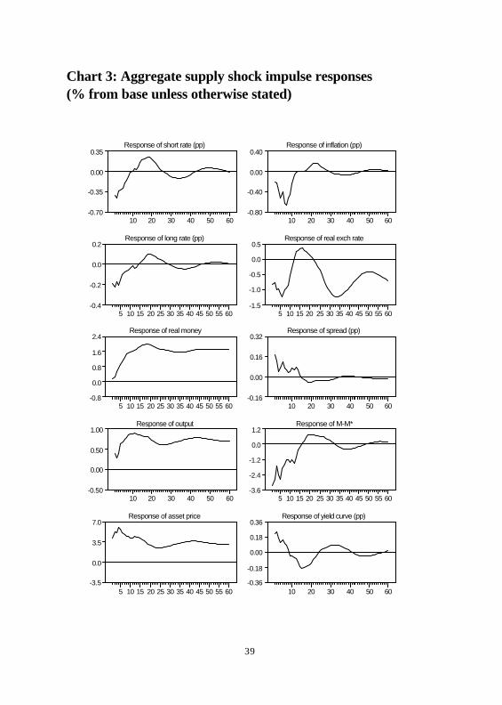
• The effects of an AS shock conform almost exactly to theory. Realmoney, output, and asset prices all rise in the long run, following asupply shock. And real asset prices initially show a tendency toovershoot their long-run equilibrium. Also, there is a negative

37

short-run effect on inflation, so that the price level falls permanently inresponse to an AS shock. The real exchange rate declines in the longrun(10). The liquidity gap, M-M*, declines initially, as income and assetprices both raise M* by more than the rise in M. So under an AS shock,M-M* is negatively associated with output, but positively associatedwith inflation.

• The effects of a nominal shock also look sensible. Short rates fall in theshort run, the real exchange rate depreciates in line with traditionalDornbusch overshooting models and inflation rises. As this shockultimately has a permanent effect on inflation, long rates rise inanticipation, so the term structure becomes upward-sloping. In the longrun, all three nominal variables converge on the same value as implied bythe stationary real interest rate. Money, real asset prices and output areboth positively affected in the short run, before tailing away to zero. Thechart shows that it is a good idea to restrict the cointegrating vectorsbefore identifying the shocks. The imposition of the term structure andstationary real interest rate cointegrating relationships ensures that allthree nominal variables are equated in the long run, in accordance withthe Fisher hypothesis. Initially, M falls slightly below M*, despite apositive effect on real balances in the short run. But after around fivequarters, a large liquidity gap emerges, which peaks at around the sametime as output and a little ahead of inflation.

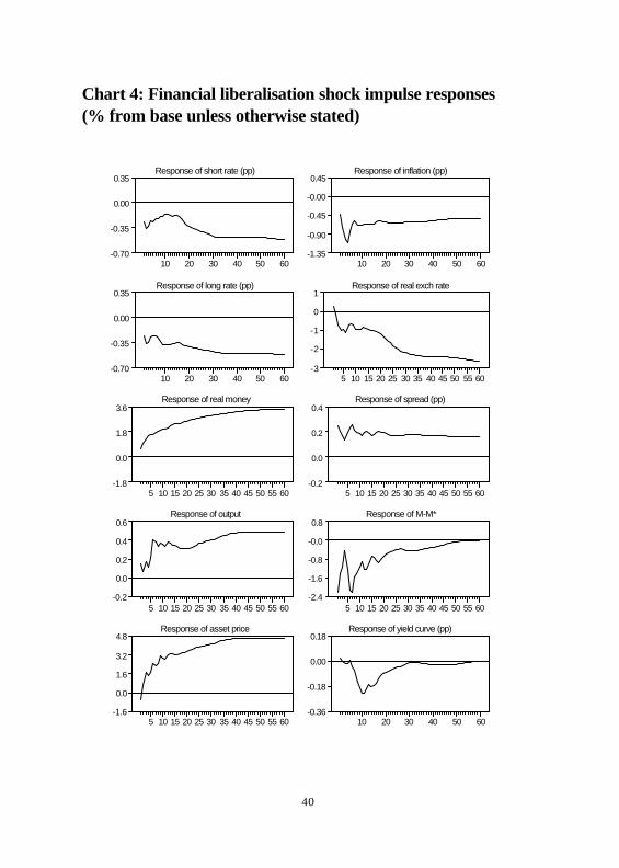
• The financial intermediation shock has a large impact on money balances,and deposit rates rise relative to short and long rates, implying a fall inthe cost of intermediation. Output rises, and both inflation and the realexchange rate fall in the long run, which is perhaps suggestive of credit-channel effects on aggregate supply. M-M* falls in the short run, asrises in output, asset prices and the spread of deposit rates over shortrates all work to increase M*. So under this shock, M-M* is negativelyrelated to output in the short run, but positively related to inflation. Thelatter may simply result from not restricting the responses of nominal

________________________________________________(10) In theory the real exchange rate declines to boost net trade sufficiently so that itmeets the rise in import demand resulting from the wealth/income generated by theproductivity increase.

38

variables to this shock to be zero.

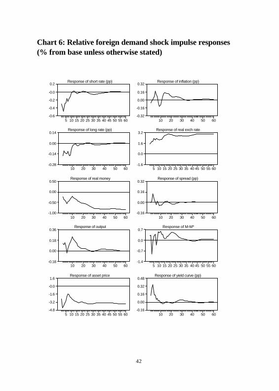
• The chief impact of the foreign shock in the long run is on the realexchange rate. But there is also a negative effect on real asset prices, asimplied by the asset-price relationship that we identified as one of thecointegrating vectors.

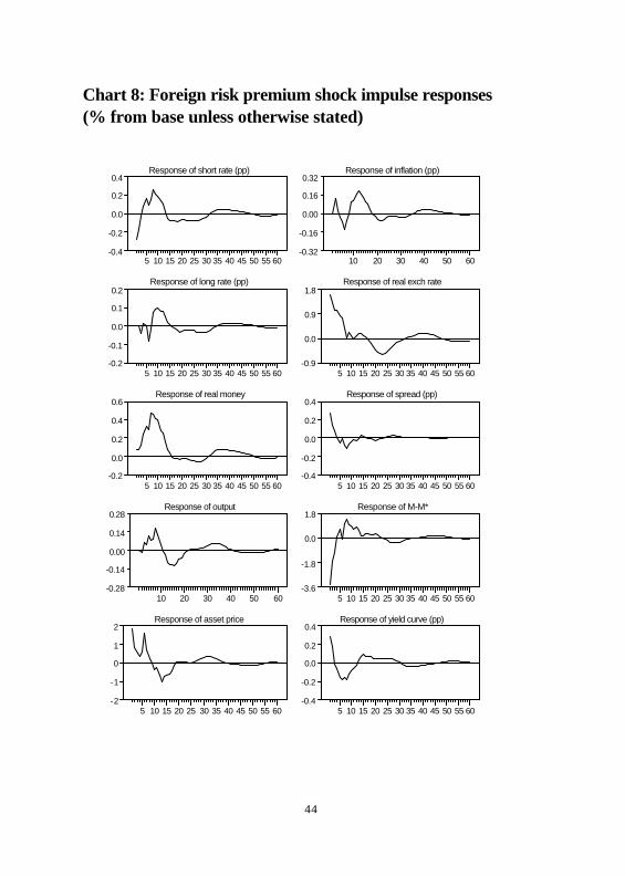
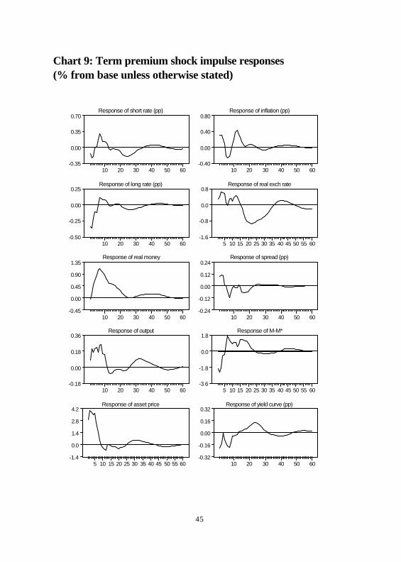
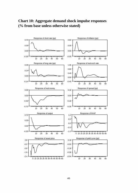
The temporary shocks

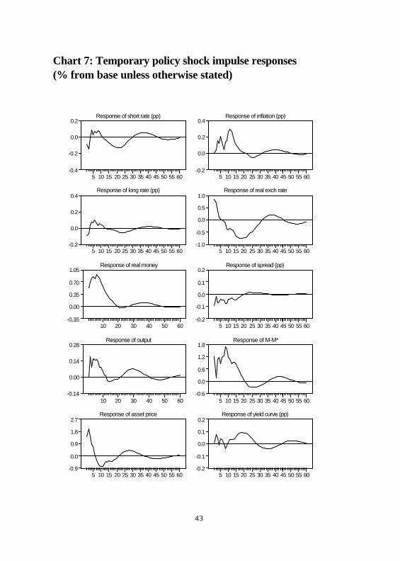
• The temporary monetary policy shock produces broadly sensibleresponses. It involves a cut in short-term interest rates, which increasesasset prices and subsequently output and inflation in the short tomedium term. So there is no ‘price puzzle’ effect. But the exchange rateinitially shows a perverse response. Only after several quarters does itdepreciate below its long-run equilibrium level as in the Dornbuschovershooting story. M-M* rises under this shock, as theory wouldpredict. And (partly by construction) it leads both output and inflationwith a positive effect.

• The responses to a domestic demand shock all accord with theory. Anexpansion of aggregate demand initially leads to a rise in interest rates bythe authorities (eg since this produces inflation inconsistent with theauthorities policy objectives) and a rise in output and the real exchangerate in the medium term.

• The impact of the foreign risk-premium shock appears to be sensible,having strong effects on real asset prices and the real exchange rate,consistent with it representing a shift in preferences towardssterling-denominated assets.

• The unrestricted shock, which we provisionally labelled a‘term-premium’ shock, would seem to live up to its name. A fall in thepremium leads to long rates falling relative to short rates, and this boostsmoney, output, asset prices and inflation in the short run.

Generally, the impulse responses are sensibly signed and provide somesupport for our identifying restrictions. In particular, neither of our monetarypolicy shocks exhibits the price puzzle problem. More interestingly, differentshocks produce different relationships between surplus liquidity and outputand inflation.

39

Chart 3: Aggregate supply shock impulse responses(% from base unless otherwise stated)

Response of short rate (pp)

10 20 30 40 50 60-0.70

-0.35

0.00

0.35

Response of long rate (pp)

5 10 15 20 25 30 35 40 45 50 55 60-0.4

-0.2

0.0

0.2

Response of real money

5 10 15 20 25 30 35 40 45 50 55 60-0.8

0.0

0.8

1.6

2.4

Response of output

10 20 30 40 50 60-0.50

0.00

0.50

1.00

Response of asset price

5 10 15 20 25 30 35 40 45 50 55 60-3.5

0.0

3.5

7.0

Response of inflation (pp)

10 20 30 40 50 60-0.80

-0.40

0.00

0.40

Response of real exch rate

5 10 15 20 25 30 35 40 45 50 55 60-1.5

-1.0

-0.5

0.0

0.5

Response of spread (pp)

10 20 30 40 50 60-0.16

0.00

0.16

0.32

Response of M-M*

5 10 15 20 25 30 35 40 45 50 55 60-3.6

-2.4

-1.2

0.0

1.2

Response of yield curve (pp)

10 20 30 40 50 60-0.36

-0.18

0.00

0.18

0.36

40

Chart 4: Financial liberalisation shock impulse responses(% from base unless otherwise stated)


10 20 30 40 50 60-0.70

-0.35

0.00

0.35


10 20 30 40 50 60-0.70

-0.35

0.00

0.35


5 10 15 20 25 30 35 40 45 50 55 60-1.8

0.0

1.8

3.6

Response of output

5 10 15 20 25 30 35 40 45 50 55 60-0.2

0.0

0.2

0.4

0.6


5 10 15 20 25 30 35 40 45 50 55 60-1.6

0.0

1.6

3.2

4.8


10 20 30 40 50 60-1.35

-0.90

-0.45

-0.00

0.45


5 10 15 20 25 30 35 40 45 50 55 60-3

-2

-1

0

1


5 10 15 20 25 30 35 40 45 50 55 60-0.2

0.0

0.2

0.4

Response of M-M*

5 10 15 20 25 30 35 40 45 50 55 60-2.4

-1.6

-0.8

-0.0

0.8


10 20 30 40 50 60-0.36

-0.18

0.00

0.18

41

Chart 5: Permanent policy shock impulse responses(% from base unless otherwise stated)


10 20 30 40 50 60-0.40

0.00

0.40

0.80


10 20 30 40 50 60-0.25

0.00

0.25

0.50

0.75


5 10 15 20 25 30 35 40 45 50 55 60-2.7

-1.8

-0.9

-0.0

0.9

Response of output

10 20 30 40 50 60-0.35

0.00

0.35

0.70


10 20 30 40 50 60-10.0

-5.0

0.0

5.0


10 20 30 40 50 60-0.40

0.00

0.40

0.80

1.20


5 10 15 20 25 30 35 40 45 50 55 60-2.7

-1.8

-0.9

-0.0

0.9


10 20 30 40 50 60-0.28

-0.14

0.00

0.14

0.28

Response of M-M*

5 10 15 20 25 30 35 40 45 50 55 60-1.6

0.0

1.6

3.2


10 20 30 40 50 60-0.16

0.00

0.16

0.32

0.48

42

Chart 6: Relative foreign demand shock impulse responses(% from base unless otherwise stated)


5 10 15 20 25 30 35 40 45 50 55 60-0.6

-0.4

-0.2

-0.0

0.2


10 20 30 40 50 60-0.28

-0.14

0.00

0.14


10 20 30 40 50 60-1.00

-0.50

0.00

0.50

Response of output

10 20 30 40 50 60-0.18

0.00

0.18

0.36


5 10 15 20 25 30 35 40 45 50 55 60-4.8

-3.2

-1.6

-0.0

1.6


10 20 30 40 50 60-0.32

-0.16

0.00

0.16

0.32


5 10 15 20 25 30 35 40 45 50 55 60-1.6

0.0

1.6

3.2


10 20 30 40 50 60-0.16

0.00

0.16

0.32

Response of M-M*

5 10 15 20 25 30 35 40 45 50 55 60-1.4

-0.7

0.0

0.7


10 20 30 40 50 60-0.16

0.00

0.16

0.32

0.48

43

Chart 7: Temporary policy shock impulse responses(% from base unless otherwise stated)


5 10 15 20 25 30 35 40 45 50 55 60-0.4

-0.2

0.0

0.2


5 10 15 20 25 30 35 40 45 50 55 60-0.2

0.0

0.2

0.4


10 20 30 40 50 60-0.35

0.00

0.35

0.70

1.05

Response of output

10 20 30 40 50 60-0.14

0.00

0.14

0.28


5 10 15 20 25 30 35 40 45 50 55 60-0.9

0.0

0.9

1.8

2.7


5 10 15 20 25 30 35 40 45 50 55 60-0.2

0.0

0.2

0.4


5 10 15 20 25 30 35 40 45 50 55 60-1.0

-0.5

0.0

0.5

1.0


5 10 15 20 25 30 35 40 45 50 55 60-0.2

-0.1

0.0

0.1

0.2

Response of M-M*

5 10 15 20 25 30 35 40 45 50 55 60-0.6

0.0

0.6

1.2

1.8


5 10 15 20 25 30 35 40 45 50 55 60-0.2

-0.1

0.0

0.1

0.2

44

Chart 8: Foreign risk premium shock impulse responses(% from base unless otherwise stated)


5 10 15 20 25 30 35 40 45 50 55 60-0.4

-0.2

0.0

0.2

0.4


5 10 15 20 25 30 35 40 45 50 55 60-0.2

-0.1

0.0

0.1

0.2


5 10 15 20 25 30 35 40 45 50 55 60-0.2

0.0

0.2

0.4

0.6

Response of output

10 20 30 40 50 60-0.28

-0.14

0.00

0.14

0.28


5 10 15 20 25 30 35 40 45 50 55 60-2

-1

0

1

2


10 20 30 40 50 60-0.32

-0.16

0.00

0.16

0.32


5 10 15 20 25 30 35 40 45 50 55 60-0.9

0.0

0.9

1.8


5 10 15 20 25 30 35 40 45 50 55 60-0.4

-0.2

0.0

0.2

0.4

Response of M-M*

5 10 15 20 25 30 35 40 45 50 55 60-3.6

-1.8

0.0

1.8


5 10 15 20 25 30 35 40 45 50 55 60-0.4

-0.2

0.0

0.2

0.4

45

Chart 9: Term premium shock impulse responses(% from base unless otherwise stated)


10 20 30 40 50 60-0.35

0.00

0.35

0.70


10 20 30 40 50 60-0.50

-0.25

0.00

0.25


10 20 30 40 50 60-0.45

0.00

0.45

0.90

1.35

Response of output

10 20 30 40 50 60-0.18

0.00

0.18

0.36


5 10 15 20 25 30 35 40 45 50 55 60-1.4

0.0

1.4

2.8

4.2


10 20 30 40 50 60-0.40

0.00

0.40

0.80


5 10 15 20 25 30 35 40 45 50 55 60-1.6

-0.8

0.0

0.8


10 20 30 40 50 60-0.24

-0.12

0.00

0.12

0.24

Response of M-M*

5 10 15 20 25 30 35 40 45 50 55 60-3.6

-1.8

0.0

1.8


10 20 30 40 50 60-0.32

-0.16

0.00

0.16

0.32

46

Chart 10: Aggregate demand shock impulse responses(% from base unless otherwise stated)


10 20 30 40 50 60-0.35

0.00

0.35

0.70


10 20 30 40 50 60-0.14

0.00

0.14

0.28


10 20 30 40 50 60-0.70

-0.35

0.00

0.35

Response of output

10 20 30 40 50 60-0.35

0.00

0.35

0.70


5 10 15 20 25 30 35 40 45 50 55 60-2.4

-1.6

-0.8

-0.0

0.8


10 20 30 40 50 60-0.30

0.00

0.30

0.60


10 20 30 40 50 60-0.45

0.00

0.45

0.90

1.35


10 20 30 40 50 60-0.36

-0.18

0.00

0.18

Response of M-M*

5 10 15 20 25 30 35 40 45 50 55 60-1.0

-0.5

0.0

0.5

1.0


10 20 30 40 50 60-0.54

-0.36

-0.18

-0.00

0.18

47

(d) Variance decomposition

An additional diagnostic on our identifying restrictions is the relativeimportance of the shocks in driving each of the variables in the system. Todo this, we carry out a variance decomposition analysis of the system.

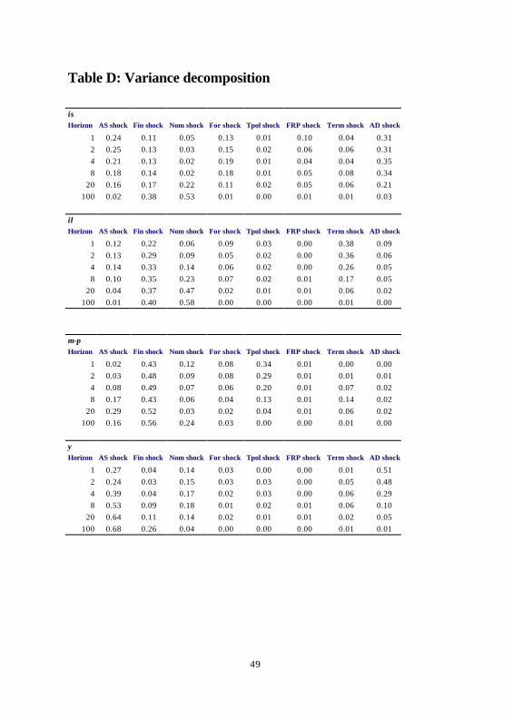
A variance decomposition analysis derives the contribution of each of theshocks to the variance of the forecast error for each variable at different timehorizons. In other words, it shows how much of the variability of each of thevariables is accounted for by each shock at different time horizons. In TableD below, we show a forecast error variance decomposition for each variable.The key points to note are:

(1) Movements in real M4 seem to be dominated at long horizons byfinancial intermediation, AS and nominal shocks. But at short horizons,temporary policy shocks appear to be quite important, suggesting thatunexpected cuts in rates may have significant effects on money growth.

(2) As in a lot of other SVAR work, movements in output are dominated byAS shocks at long horizons. But at short horizons, AD shocks accountfor a large proportion of output movements. Nominal shocks do appearto have a significant effect on output, suggesting that there may besubstantial costs of moving to a lower steady-state rate of inflation.Temporary policy shocks account for a small proportion (around 3%) ofoutput variability at short horizons.

(3) Interest rates, though largely determined by nominal shocks in the longrun, appear to be affected by most of the shocks to a fairly equal degreein the short run. The only exception is the temporary policy shocks,which only account for around 1% of the short-term variability in rates.This suggests that deviations from some average policy rule have beensmall. But it might also suggest that temporary policy shocks are beingcaptured by one of the other temporary shocks.

(4) Around one quarter of the variability in deposit rates at long horizons isaccounted for by financial intermediation shocks. And the term-premiumshock has a large impact on long rates at short horizons. This supportsour interpretation of the unrestricted shocks.

48

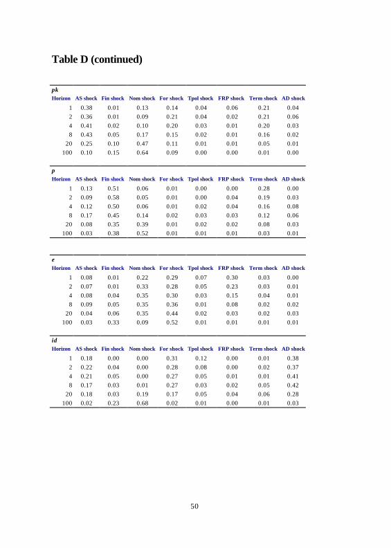
(5) More than half the variability in the real exchange rate at long horizons isdue to foreign demand shocks, giving us some confidence in ouridentifying restrictions on this variable. By contrast, AD shocks, as wehave identified them, appear to have little effect, even in the short run.This contrasts with other studies that have attempted a SVARdecomposition of the exchange rate (eg Astley and Garratt (1998)), whichusually find IS or demand shocks to have an important role in explainingexchange rate movements. But the important point to stress here is thatthe restrictions we place on the relative foreign demand shock are verysimilar to those typically used to identify AD shocks, as we discussedearlier. In effect, we have split general demand shocks into two subsets:a temporary domestic demand shock and a permanent relative foreigndemand shock. The latter appears to be more important in explainingexchange rate movements.

(6) Although inflation is dominated in the long run by the permanent policy

shock, financial liberalisation shocks seem to have an implausibly largerole in determining short to medium-term movements in inflation. Thissuggests that further over-identifying restrictions may be necessary torecover this shock fully.

49

Table D: Variance decomposition

isHorizon AS shock Fin shock Nom shock For shock Tpol shock FRP shock Term shock AD shock

1 0.24 0.11 0.05 0.13 0.01 0.10 0.04 0.312 0.25 0.13 0.03 0.15 0.02 0.06 0.06 0.314 0.21 0.13 0.02 0.19 0.01 0.04 0.04 0.358 0.18 0.14 0.02 0.18 0.01 0.05 0.08 0.34

20 0.16 0.17 0.22 0.11 0.02 0.05 0.06 0.21100 0.02 0.38 0.53 0.01 0.00 0.01 0.01 0.03

ilHorizon AS shock Fin shock Nom shock For shock Tpol shock FRP shock Term shock AD shock

1 0.12 0.22 0.06 0.09 0.03 0.00 0.38 0.092 0.13 0.29 0.09 0.05 0.02 0.00 0.36 0.064 0.14 0.33 0.14 0.06 0.02 0.00 0.26 0.058 0.10 0.35 0.23 0.07 0.02 0.01 0.17 0.05

20 0.04 0.37 0.47 0.02 0.01 0.01 0.06 0.02100 0.01 0.40 0.58 0.00 0.00 0.00 0.01 0.00

m-pHorizon AS shock Fin shock Nom shock For shock Tpol shock FRP shock Term shock AD shock

1 0.02 0.43 0.12 0.08 0.34 0.01 0.00 0.002 0.03 0.48 0.09 0.08 0.29 0.01 0.01 0.014 0.08 0.49 0.07 0.06 0.20 0.01 0.07 0.028 0.17 0.43 0.06 0.04 0.13 0.01 0.14 0.02

20 0.29 0.52 0.03 0.02 0.04 0.01 0.06 0.02100 0.16 0.56 0.24 0.03 0.00 0.00 0.01 0.00

yHorizon AS shock Fin shock Nom shock For shock Tpol shock FRP shock Term shock AD shock

1 0.27 0.04 0.14 0.03 0.00 0.00 0.01 0.512 0.24 0.03 0.15 0.03 0.03 0.00 0.05 0.484 0.39 0.04 0.17 0.02 0.03 0.00 0.06 0.298 0.53 0.09 0.18 0.01 0.02 0.01 0.06 0.10

20 0.64 0.11 0.14 0.02 0.01 0.01 0.02 0.05100 0.68 0.26 0.04 0.00 0.00 0.00 0.01 0.01

50

Table D (continued)

pkHorizon AS shock Fin shock Nom shock For shock Tpol shock FRP shock Term shock AD shock

1 0.38 0.01 0.13 0.14 0.04 0.06 0.21 0.042 0.36 0.01 0.09 0.21 0.04 0.02 0.21 0.064 0.41 0.02 0.10 0.20 0.03 0.01 0.20 0.038 0.43 0.05 0.17 0.15 0.02 0.01 0.16 0.02

20 0.25 0.10 0.47 0.11 0.01 0.01 0.05 0.01100 0.10 0.15 0.64 0.09 0.00 0.00 0.01 0.00

πHorizon AS shock Fin shock Nom shock For shock Tpol shock FRP shock Term shock AD shock

1 0.13 0.51 0.06 0.01 0.00 0.00 0.28 0.002 0.09 0.58 0.05 0.01 0.00 0.04 0.19 0.034 0.12 0.50 0.06 0.01 0.02 0.04 0.16 0.088 0.17 0.45 0.14 0.02 0.03 0.03 0.12 0.06

20 0.08 0.35 0.39 0.01 0.02 0.02 0.08 0.03100 0.03 0.38 0.52 0.01 0.01 0.01 0.03 0.01

eHorizon AS shock Fin shock Nom shock For shock Tpol shock FRP shock Term shock AD shock

1 0.08 0.01 0.22 0.29 0.07 0.30 0.03 0.002 0.07 0.01 0.33 0.28 0.05 0.23 0.03 0.014 0.08 0.04 0.35 0.30 0.03 0.15 0.04 0.018 0.09 0.05 0.35 0.36 0.01 0.08 0.02 0.02

20 0.04 0.06 0.35 0.44 0.02 0.03 0.02 0.03100 0.03 0.33 0.09 0.52 0.01 0.01 0.01 0.01

idHorizon AS shock Fin shock Nom shock For shock Tpol shock FRP shock Term shock AD shock

1 0.18 0.00 0.00 0.31 0.12 0.00 0.01 0.382 0.22 0.04 0.00 0.28 0.08 0.00 0.02 0.374 0.21 0.05 0.00 0.27 0.05 0.01 0.01 0.418 0.17 0.03 0.01 0.27 0.03 0.02 0.05 0.42

20 0.18 0.03 0.19 0.17 0.05 0.04 0.06 0.28100 0.02 0.23 0.68 0.02 0.01 0.00 0.01 0.03

51

4 Practical uses of the model

(a) Generating output gaps and liquidity overhangs

One obvious use of the model is to generate trend levels for each of thevariables, using the common stochastic trends we have identified. At firstglance this seems straightforward. We simply use the long-run impact matrixof the shocks, F, to generate a trend for each variable that is a linearcombination of the stochastic trends that drive that variable in the long run.

But we must be careful here, as use of the word ‘trend’ means different thingsin different contexts. In particular, there may be circumstances when the trendwe wish to construct would include the cyclical effects of some of thepermanent shocks. A good example is the output gap. The concept of the‘trend’ level of output used to construct an output gap is typically somenotion of the supply capacity of the economy. In this case, we would want toinclude the cyclical effects of productivity shocks on output, since theseclearly affect the supply capacity of the economy at a given moment in time.To put this another way, we would want our output gap to reflect shocks thatonly have a temporary effect on output, such as aggregate demand andmonetary policy shocks.

Another good example is that of estimating the trend in inflation or ‘core’inflation. Do we want to include the ‘cyclical’ or dynamic effects of thenominal stochastic trend? One way to answer this question is to say ‘no’ ifwe are after a measure of the underlying inflation or nominal target of theauthorities; but ‘yes’ if we are after a measure of inflation expectations thatwould enter an expectations-augmented Phillip’s curve, for example. Thedynamic effects of a change in the nominal trend/inflation target could beinterpreted as the adjustment of inflation expectations as the private sectorlearns about a new regime. Chart 11 below shows these two differentmeasures of core inflation. Core 2, which includes the cyclical effects of thenominal shock, shows less variation than Core 1, which excludes theseeffects. This could be interpreted as partial adjustment of inflationexpectations to changes in the underlying target.

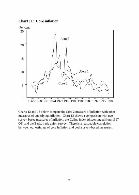
52

Chart 11: Core inflation

Charts 12 and 13 below compare the Core 2 measure of inflation with othermeasures of underlying inflation. Chart 13 shows a comparison with twosurvey-based measures of inflation, the Gallup index (discontinued from 1997Q3) and the Basix trade union survey. There is a reasonable correlationbetween our estimate of core inflation and both survey-based measures.

1965 1968 1971 1974 1977 1980 1983 1986 1989 1992 1995 19980

5

10

15

20

25

Actual

Core 1

Core 2

Per cent

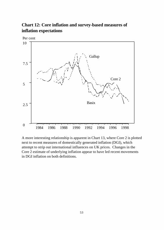
53

Chart 12: Core inflation and survey-based measures ofinflation expectations

A more interesting relationship is apparent in Chart 13, where Core 2 is plottednext to recent measures of domestically generated inflation (DGI), whichattempt to strip out international influences on UK prices. Changes in theCore 2 estimate of underlying inflation appear to have led recent movementsin DGI inflation on both definitions.

Core 2

1984 1986 1988 1990 1992 1994 1996 19980

2.5

5

7.5

10

Basix

Gallup

Per cent

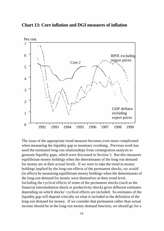
54

Chart 13: Core inflation and DGI measures of inflation

The issue of the appropriate trend measure becomes even more complicatedwhen measuring the liquidity gap or monetary overhang. Previous work hasused the estimated long-run relationships from cointegration analysis togenerate liquidity gaps, which were discussed in Section 3. But this measuresequilibrium money holdings when the determinants of the long-run demandfor money are at their actual levels. If we were to take the trend in moneyholdings implied by the long-run effects of the permanent shocks, we would(in effect) be measuring equilibrium money holdings when the determinants ofthe long-run demand for money were themselves at their trend level.Including the cyclical effects of some of the permanent shocks (such as thefinancial intermediation shock or productivity shock) gives different estimatesdepending on which shocks’ cyclical effects are included. So estimates of theliquidity gap will depend critically on what is included in the definition of thelong-run demand for money. If we consider that permanent rather than actualincome should be in the long-run money demand function, we should go for a

1992 1993 1994 1995 1996 1997 1998 19990

1

2

3

4

5

6

7

Core 2

GDP deflatorexcludingexport prices

RPIX excludingimport prices

Per cent

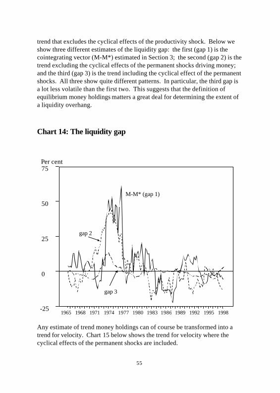
55

trend that excludes the cyclical effects of the productivity shock. Below weshow three different estimates of the liquidity gap: the first (gap 1) is thecointegrating vector (M-M*) estimated in Section 3; the second (gap 2) is thetrend excluding the cyclical effects of the permanent shocks driving money;and the third (gap 3) is the trend including the cyclical effect of the permanentshocks. All three show quite different patterns. In particular, the third gap isa lot less volatile than the first two. This suggests that the definition ofequilibrium money holdings matters a great deal for determining the extent ofa liquidity overhang.

Chart 14: The liquidity gap

Any estimate of trend money holdings can of course be transformed into atrend for velocity. Chart 15 below shows the trend for velocity where thecyclical effects of the permanent shocks are included.

1965 1968 1971 1974 1977 1980 1983 1986 1989 1992 1995 1998-25

0

25

50

75

M-M* (gap 1)

gap 2

gap 3

Per cent

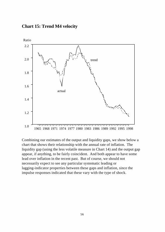
56

Chart 15: Trend M4 velocity

Combining our estimates of the output and liquidity gaps, we show below achart that shows their relationship with the annual rate of inflation. Theliquidity gap (using the less volatile measure in Chart 14) and the output gapappear, if anything, to be fairly coincident. And both appear to have somelead over inflation in the recent past. But of course, we should notnecessarily expect to see any particular systematic leading orlagging-indicator properties between these gaps and inflation, since theimpulse responses indicated that these vary with the type of shock.

1965 1968 1971 1974 1977 1980 1983 1986 1989 1992 1995 19981.0

1.2

1.4

1.6

1.8

2.0

2.2

trend

actual

Ratio

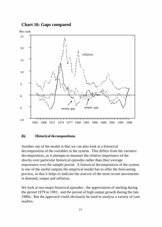
57

Chart 16: Gaps compared

(b) Historical decompositions

Another use of the model is that we can also look at a historicaldecomposition of the variables in the system. This differs from the variancedecomposition, as it attempts to measure the relative importance of theshocks over particular historical episodes rather than their averageimportance over the sample period. A historical decomposition of the systemis one of the useful outputs the empirical model has to offer the forecastingprocess, in that it helps to indicate the sources of the most recent movementsin demand, output and inflation.

We look at two major historical episodes: the appreciation of sterling duringthe period 1979 to 1981; and the period of high output growth during the late1980s. But the approach could obviously be used to analyse a variety of casestudies.

1965 1968 1971 1974 1977 1980 1983 1986 1989 1992 1995 1998-10

-5

0

5

10

15

20

25

inflation

money gap output gap

Per cent

58

The appreciation of sterling 1979-81— oil or monetary policy ?

Between 1979 Q2 and 1981 Q1 the real value of sterling in terms of relative unitlabour costs rose by almost 40%. At the time there was considerable debateover whether this rise in the real exchange rate was driven by: (i) the impactof higher oil prices on the trade balance, since the United Kingdom hadbecome a net exporter of oil by the late 1970s; or (ii) the restrictive monetarypolicy implemented by the incoming Conservative government designed tolower the underlying rate of inflation. Buiter and Miller (1981) showed thatboth shocks might cause an overshooting of the real exchange rate in theshort run and, in the case of oil, a permanent rise in the equilibrium realexchange rate in the long run.

In terms of the VAR we can attempt to shed light on this issue by analysingthe contributions of the various structural shocks to exchange ratemovements over this period. A strong contribution from the aggregatesupply shock or possibly the relative foreign demand shock would suggestthe oil price was more responsible for the rise in the real exchange rate. Astrong contribution from the permanent nominal shock, on the other hand,would suggest that restrictive monetary policy was the chief driving force.

Chart 17 below shows the cumulative rise in the real exchange rate between1979 Q2 and 1981 Q1 relative to the cumulative contribution of each of thestructural shocks. The decomposition suggests that around a third of the risemight be explained by the permanent monetary policy shock, while at mostanother third could be attributable to oil through the aggregate supply andrelative foreign demand shocks.

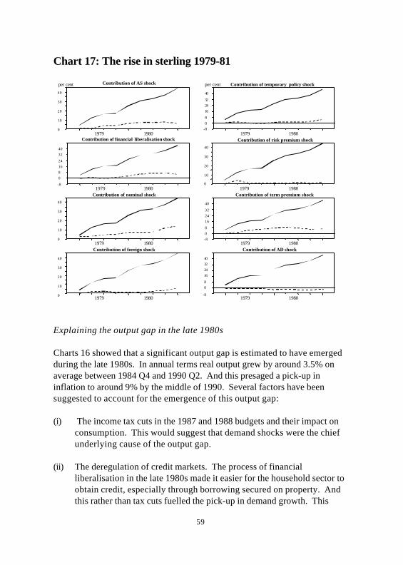
59

Chart 17: The rise in sterling 1979-81

Explaining the output gap in the late 1980s

Charts 16 showed that a significant output gap is estimated to have emergedduring the late 1980s. In annual terms real output grew by around 3.5% onaverage between 1984 Q4 and 1990 Q2. And this presaged a pick-up ininflation to around 9% by the middle of 1990. Several factors have beensuggested to account for the emergence of this output gap:

(i) The income tax cuts in the 1987 and 1988 budgets and their impact onconsumption. This would suggest that demand shocks were the chiefunderlying cause of the output gap.

(ii) The deregulation of credit markets. The process of financialliberalisation in the late 1980s made it easier for the household sector toobtain credit, especially through borrowing secured on property. Andthis rather than tax cuts fuelled the pick-up in demand growth. This

Contribution of AS shock

1979 19800

10

20

30

40

Contribution of financial liberalisation shock

1979 1980-8

081624

3240

Contribution of nominal shock

1979 19800

10

20

30

40

Contribution of foreign shock

1979 19800

10

20

30

40

Contribution of temporary policy shock

1979 1980-808

162432

40

Contribution of risk premium shock

1979 19800

10

20

30

40

Contribution of term premium shock

1979 1980-808

162432

40

Contribution of AD shock

1979 1980-8

08

16243240

per cent per cent

60

would suggest that financial liberalisation shocks had a significanteffect on demand and output.

(iii) Shadowing the Deutsche Mark. Over this period the Chancellorattempted, either formally or informally, to keep sterling tied to theDeutsche Mark. Even though it was argued that this would lock theUnited Kingdom into Germany’s low inflation rate, the upward pressureon sterling at the time may have forced the authorities to lead too loosea monetary policy, with the implication that the underlying rate ofnominal expansion or implicit inflation target may have risen. Forexample there may have been a rise in the equilibrium real exchange ratewhich put upward pressure on sterling. And in response the authoritiesheld interest rates at relatively low levels to prevent the nominalexchange rate from rising. The resulting fall in real interest rates andbuild-up of a liquidity overhang would then explain the expansion ofaggregate demand and the emergence of an output gap. This argumentwould suggest that the output gap was driven primarily by permanentmonetary policy shocks, possibly with a contribution from relativeforeign demand shocks which pushed up the equilibrium real exchangerate.

Chart 18 below shows the cumulative rise in the output gap (which wemeasure here as the cumulative rise in output excluding the cumulative impactof aggregate supply or productivity shocks) relative to the contribution ofeach of the shocks from 1984 Q4 to 1990 Q2.

• Aggregate demand shocks appear to have some role in sustaining theoutput gap during 1988 but their cumulative effect diminishes in 1989and 1990. So on this evidence tax cuts would appear to have had a smalltransitory role in boosting demand and output.

• Financial liberalisation shocks have a small but more persistent effect onthe output gap, suggesting at least some impact of financialderegulation on demand. An examination of the historicaldecomposition of real money balances over this period shows a muchstronger contribution from financial liberalisation, suggesting a strongshift in trend velocity.

• Permanent nominal shocks seem to have made the most importantcontribution to the output gap, at least to the height of the boom in 1988

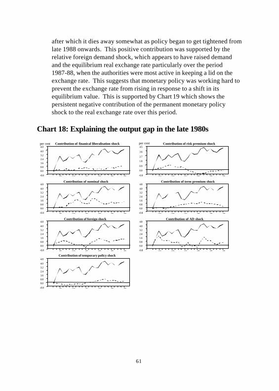
61

after which it dies away somewhat as policy began to get tightened fromlate 1988 onwards. This positive contribution was supported by therelative foreign demand shock, which appears to have raised demandand the equilibrium real exchange rate particularly over the period1987-88, when the authorities were most active in keeping a lid on theexchange rate. This suggests that monetary policy was working hard toprevent the exchange rate from rising in response to a shift in itsequilibrium value. This is supported by Chart 19 which shows thepersistent negative contribution of the permanent monetary policyshock to the real exchange rate over this period.

Chart 18: Explaining the output gap in the late 1980s

Contribution of finanical liberalisation shock

1985 1 9 8 6 1987 1988 1989 1990-0.8

0.00.81.62.43.24.0

4.8

Contribution of nominal shock

1985 1 9 8 6 1987 1988 1989 1990-0.8

0.00.81.62.43.24.0

4.8

Contribution of foreign shock

1985 1 9 8 6 1987 1988 1989 1990-0.8

0.00.81.62.43.24.0

4.8

Contribution of temporary policy shock

1985 1 9 8 6 1987 1988 1989 1990-0.8

0.00.81.62.43.24.0

4.8

Contribution of risk premium shock

1 9 8 5 1986 1987 1988 1989 1990-0.9

0.0

0.9

1.8

2.7

3.6

4.5

Contribution of term premium shock

1 9 8 5 1986 1987 1988 1989 1990-0.8

0.00.81.62.43.24.0

4.8

Contribution of AD shock

1 9 8 5 1986 1987 1988 1989 1990-0.8

0.00.81.62.43.24.0

4.8

per cent per cent

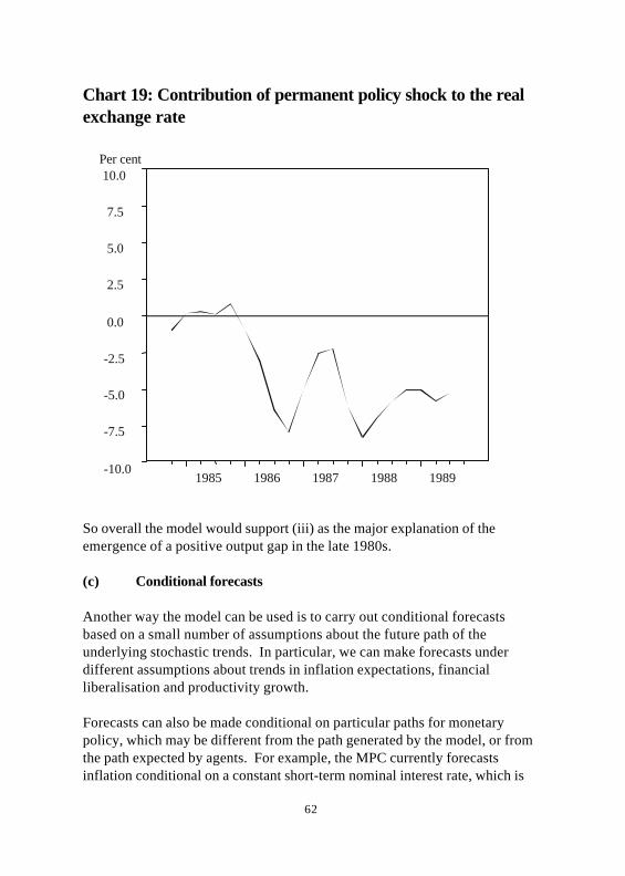
62

Chart 19: Contribution of permanent policy shock to the realexchange rate

So overall the model would support (iii) as the major explanation of theemergence of a positive output gap in the late 1980s.

(c) Conditional forecasts

Another way the model can be used is to carry out conditional forecastsbased on a small number of assumptions about the future path of theunderlying stochastic trends. In particular, we can make forecasts underdifferent assumptions about trends in inflation expectations, financialliberalisation and productivity growth.

Forecasts can also be made conditional on particular paths for monetarypolicy, which may be different from the path generated by the model, or fromthe path expected by agents. For example, the MPC currently forecastsinflation conditional on a constant short-term nominal interest rate, which is

1985 1986 1987 1988 1989-10.0

-7.5

-5.0

-2.5

0.0

2.5

5.0

7.5

10.0Per cent

63

typically different from the path implied by interest rate futures or bondyields. In the context of our model, conditioning on a path for the interest ratethat differed from the path predicted by the model would imply a series ofmonetary policy surprises over the forecast period, ie we would forecastconditional on a path for the monetary policy shocks. The important issuehere is one of signal extraction. In the light of interest rates turning outdifferently from expected, how much do agents assume that this is atemporary policy shock and how much a permanent shift in the nominal targetof the authorities? We intend to examine some of these issues in future work.

5 Conclusions

We have estimated a small structural model, involving eight variables thattheory predicts play an important role in the monetary policy transmissionmechanism. We found that we were able to decompose movements in thesevariables into four permanent and four temporary shocks, each of which wasidentified according to economic criteria. The properties of the model seembroadly sensible, and there do not seem to be any ‘price puzzle’ problemswith the response of inflation to either permanent or temporary monetarypolicy shocks. But there are some features of the model (eg the impact of thefinancial liberalisation shocks on inflation) that we intend to look at further infuture work. The model also builds on previous work in the Bank, by showingexplicitly how different shocks produce a different interaction between moneyholdings, monetary overhangs, activity and prices.

We have also shown some of the practical uses of such a model. The modelcan be used to produce estimates of the output gap, liquidity gap, and coreinflation. It can also be used to identify which shocks have been the mostimportant in driving each of the variables over a given time period. Perhapsmore importantly, the model can also be used to provide conditionalforecasts, based on different assumptions about the future paths of thestochastic trends and temporary shocks.

64

References

Astley, M and Garratt, A (1998), ‘Exchange rates and prices: sources ofsterling real exchange rate fluctuations 1973-94’, Bank of England WorkingPaper, No 85.

Bank of England (1999), Economic models at the Bank of England.

Blanchard, O J (1981), ‘Output, the stock market, and interest rates’,American Economic Review, 71(1), March 1981, pages 132-43.

Brigden, A and Mizen, P (1999), ‘Money, credit and investment in the UKcorporate sector’, Bank of England Working Paper, No 100.

Buiter, W H and Miller, M (1981), ‘Monetary policy and internationalcompetitiveness: the problems of adjustment’, Oxford EconomicPapers, 33,Supplement July 1981, pages 143-75.

Dhar, S and Millard, S (2000), ‘A limited participation model of the monetarytransmission mechanism in the United Kingdom’, Bank of England WorkingPaper, forthcoming.

Doornik, J and Hansen, H (1984), ‘A practical test of multivariate normality’.Unpublished manuscript, Nuffield College, Oxford.

Dornbusch, R (1976), ‘Expectations and exchange rate dynamics’, Journal ofPolitical Economy, Vol 84(6), pages 1,161-76.

Engle, R F (1982), ‘Autoregressive conditional heteroscedasticity, withestimates of the variance of United Kingdom inflations’, Econometrica, 50,pages 987-1007.

Engle, R F and Granger, W J (1987), ‘Co-integration and error correction:representation, estimation, and testing’, in Harvey, A (ed), ‘Time series,Volume 1’.

65

Engle, R F and Yoo, B S (1991), ‘Forecasting and testing in co-integratedsystems’, in Engle, R F and Granger, C W (eds), ‘Long-run economicrelationships: Readings in cointegration.’

Fischer, S (1983), ‘A framework for monetary and banking analysis’,Economic Journal, Supplement, pages 1-16.

Hallman, J, Porter, R and Small, D (1991), ‘Is the price level tied to the M2monetary aggregate in the long run?’, American Economic Review, pages841-58.

Johansen, S (1988), ‘Statistical analysis of cointegrating vectors’, Journal ofEconomics, Dynamics and Control, pages 231-54.

Johansen, S and Juselius, K (1994), ‘Identification of the long-run andshort-run structure: an application to the IS-LM model’, Journal ofEconometrics, pages 7-36.

King, R G, Plosser, C I, Stock, J H and Watson, M W (1991), ‘Stochastictrends and economic fluctuations’, American Economic Review, pages819-40.

Mellander, E, Vredin, A and Warne, A (1992), ‘Stochastic trends andeconomic fluctuations in a small open economy’, Journal of AppliedEconometrics,Vol 7(4), pages 369-94.

Obstfeld, M and Rogoff, K (1996), ‘Foundations of internationalmacroeconomics’, MIT Press.

Pesaran, M H and Shin, Y (1995), ‘Long-run structural modelling’, Universityof Cambridge Department of Applied Economics Working Paper Series,No 9419.

Rose, A K (1988), ‘Is the real interest rate stable?’, Journal of Finance,Vol 43(5), pages 1,095-112.

66

Thomas, R S J (1997a), ‘The Demand for M4: a sectoral analysis.Part 1 - The personal sector’, Bank of England Working Paper, No 61.

Thomas, R S J (1997b), ‘The Demand for M4: a sectoral analysis.Part 2 - The corporate sector’, Bank of England Working Paper, No 62.

Thomas, R S J (1997c), ‘M, M* and M-M*: an explanation’, Bank ofEngland, mimeo.

Warne, A (1991), ‘A common trends model: identification, estimation andasymptotics’, mimeo, Stockholm School of Economics, Sweden.

White, H (1980), ‘A heteroscedastic-consistent covariance matrix estimatorand a direct test for heteroscedasticty’, Econometrica, 48, pages 817-38.

Wickens, M R (1996), ‘Interpreting cointegrating vectors and commonstochastic trends’, Journal of Econometrics, pages 255-71.

Documents

A small structural empirical model of the UK monetary