A Single Packer Method for Characterizing Water

University of ConnecticutOpenCommons@UConn

Master's Theses University of Connecticut Graduate School

1-24-2017

A Single Packer Method for Characterizing WaterContributing Fractures in Crystalline BedrockWellsNeil FlahiveUniversity of Connecticut - Storrs, [email protected]

This work is brought to you for free and open access by the University of Connecticut Graduate School at OpenCommons@UConn. It has beenaccepted for inclusion in Master's Theses by an authorized administrator of OpenCommons@UConn. For more information, please [email protected].

Recommended CitationFlahive, Neil, "A Single Packer Method for Characterizing Water Contributing Fractures in Crystalline Bedrock Wells" (2017). Master'sTheses. 1043.https://opencommons.uconn.edu/gs_theses/1043

http://lib.uconn.edu/



https://opencommons.uconn.edu

https://opencommons.uconn.edu/gs_theses

https://opencommons.uconn.edu/gs

mailto:[email protected]

A Single Packer Method for Characterizing Water Contributing

Fractures in Crystalline Bedrock Wells

Neil A. Flahive

B.S., University of Connecticut, 2013

A Thesis

Submitted in Partial Fulfillment of the

Requirements for the Degree of

Master of Science

At the

University of Connecticut

2017

ii

APPROVAL PAGE

Master of Science Thesis

A Single Packer Method for Characterizing Water Contributing Fractures in

Crystalline Bedrock Wells

Presented by

Neil A. Flahive, B.S.

Major Advisor__________________________________________________________________

Gary Robbins

Associate Advisor_______________________________________________________________

Glenn Warner

Associate Advisor_______________________________________________________________

Meredith Metcalf

University of Connecticut

2017

iii

Acknowledgements Foremost, I would like to express my gratitude to my advisor Dr. Gary Robbins, whose

enthusiasm and dedication to my research made this possible. For the continuous guidance and

support throughout my graduate career, thank you. Your imprinted wisdom, passion, and humor

will leave with me as I move forward in life.

I would also like to thank the associate members on my advisory committee, Dr. Glenn

Warner and Dr. Meredith Metcalf, for their support and interest in my research. Thank you to my

fellow graduate students, Sarah Vitale and Stephanie Phillips, for your dependability and

assistance throughout this research. In addition, I want to thank the USGS Office of

Groundwater, Branch of Geophysics, for allowing access to the wells on site in order for this

research to be conducted.

Finally, I would like to extend a special thanks to my parents, Paul and Eileen and to my

brother, Richard for their unending support, love, and encouragement in all my endeavors. This

thesis is dedicated to you.

iv

TABLE OF CONTENTS

Approval Page ................................................................................................................................. ii

Acknowledgements ........................................................................................................................ iii

Table of Contents ........................................................................................................................... iv

Table of Tables ............................................................................................................................... v

Table of Figures ............................................................................................................................. vi

Abstract ......................................................................................................................................... vii

Introduction ..................................................................................................................................... 1

Conceptual Methodology ................................................................................................................ 7

Methodology ................................................................................................................................... 9

Results and Discussion ................................................................................................................. 12

Conclusion .................................................................................................................................... 17

References ..................................................................................................................................... 18

Appendices…………………………………………………………………………………………………………….………CD-ROM

v

Table of Tables

Table 1: SIMA 1 & SIMA 2 Water Transmissive Fractures .......................................................20

Table 2: SIMA 1 – Fracture Heads and Transmissivities ............................................................20

Table 3: SIMA 2 – Fracture Heads and Transmissivities ............................................................20

Table 4: BGAS 1, BGAS 2, & BGAS 3 Water Transmissive Fractures .....................................21

Table 5: BGAS 1 – Fracture Heads and Transmissivities ...........................................................21



vi

Table of Figures

Figure 1: Conceptual Well Cross Section ....................................................................................23

Figure 2: Conceptual Well Cross Section Packer at Depth B ......................................................24

Figure 3: Conceptual Well Cross Section Packer at Depth C ......................................................25

Figure 4: Conceptual Well Cross Section Packer at Depth D .....................................................26

Figure 5: Location of Coventry Quadrangle ................................................................................27

Figure 6: Generalized Bedrock Geologic Map of Coventry Quadrangle ....................................28

Figure 7: Site Map of Beach Hall ................................................................................................29

Figure 8: Site Map of UConn Depot Campus ..............................................................................30

Figure 9: Single Packer Apparatus ..............................................................................................30

Figure 10: Graph of Water Level Recovery Data ........................................................................31

Figure 11: Type Curve Matching Water Level Displacement Data ............................................32

Figure 12: Hydraulic Profile of SIMA 1 ......................................................................................33

Figure 13: Hydraulic Profile of SIMA 2 ......................................................................................34

Figure 14: Hydraulic Profile of BGAS 1 .....................................................................................35



Figure 17: Water Level Contour Maps of BGAS Wells ..............................................................38

vii

Abstract

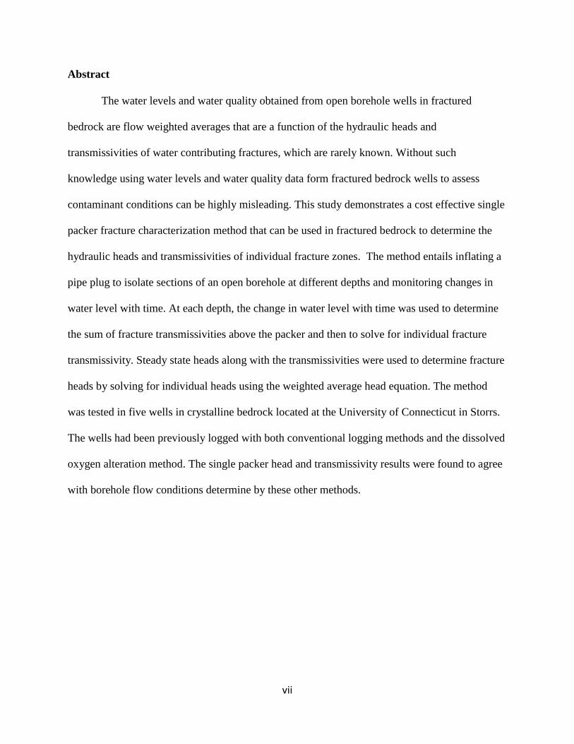
The water levels and water quality obtained from open borehole wells in fractured

bedrock are flow weighted averages that are a function of the hydraulic heads and

transmissivities of water contributing fractures, which are rarely known. Without such

knowledge using water levels and water quality data form fractured bedrock wells to assess

contaminant conditions can be highly misleading. This study demonstrates a cost effective single

packer fracture characterization method that can be used in fractured bedrock to determine the

hydraulic heads and transmissivities of individual fracture zones. The method entails inflating a

pipe plug to isolate sections of an open borehole at different depths and monitoring changes in

water level with time. At each depth, the change in water level with time was used to determine

the sum of fracture transmissivities above the packer and then to solve for individual fracture

transmissivity. Steady state heads along with the transmissivities were used to determine fracture

heads by solving for individual heads using the weighted average head equation. The method

was tested in five wells in crystalline bedrock located at the University of Connecticut in Storrs.

The wells had been previously logged with both conventional logging methods and the dissolved

oxygen alteration method. The single packer head and transmissivity results were found to agree

with borehole flow conditions determine by these other methods.

1

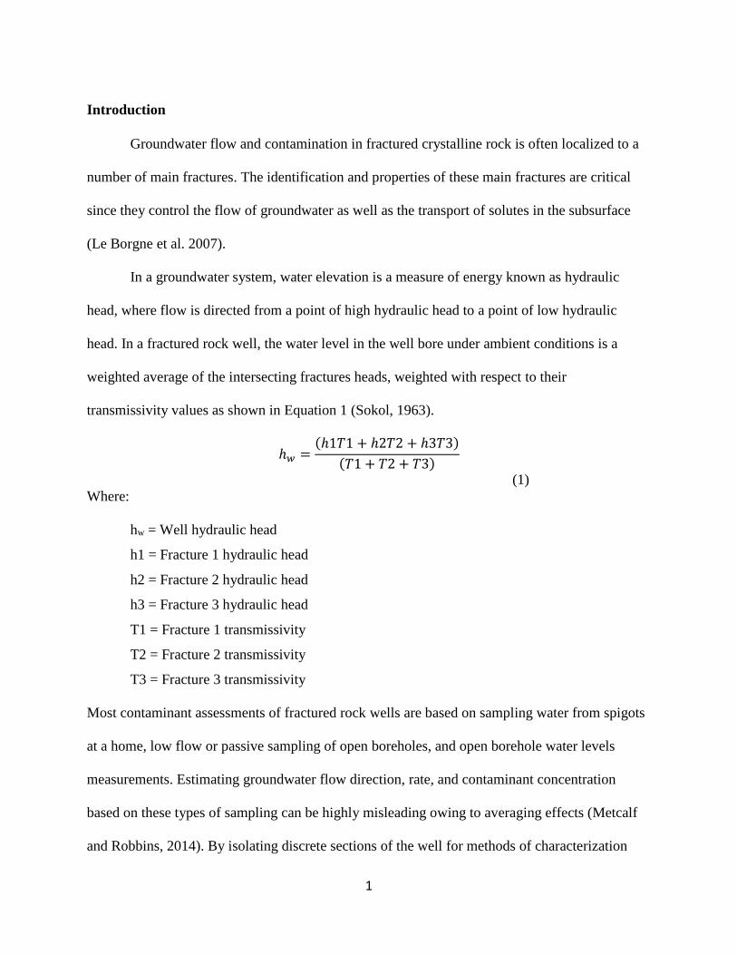
Introduction

Groundwater flow and contamination in fractured crystalline rock is often localized to a

number of main fractures. The identification and properties of these main fractures are critical

since they control the flow of groundwater as well as the transport of solutes in the subsurface

(Le Borgne et al. 2007).

In a groundwater system, water elevation is a measure of energy known as hydraulic

head, where flow is directed from a point of high hydraulic head to a point of low hydraulic

head. In a fractured rock well, the water level in the well bore under ambient conditions is a

weighted average of the intersecting fractures heads, weighted with respect to their

transmissivity values as shown in Equation 1 (Sokol, 1963).

ℎ𝑤 =(ℎ1𝑇1 + ℎ2𝑇2 + ℎ3𝑇3)

(𝑇1 + 𝑇2 + 𝑇3)

(1)

Where:

hw = Well hydraulic head

h1 = Fracture 1 hydraulic head



T1 = Fracture 1 transmissivity



Most contaminant assessments of fractured rock wells are based on sampling water from spigots

at a home, low flow or passive sampling of open boreholes, and open borehole water levels

measurements. Estimating groundwater flow direction, rate, and contaminant concentration

based on these types of sampling can be highly misleading owing to averaging effects (Metcalf

and Robbins, 2014). By isolating discrete sections of the well for methods of characterization

2

and sampling, the effects of an open borehole on hydraulic and chemical data are eliminated

(Shapiro, 2001). As such, the development of a conceptual model of groundwater flow and

solute transport in such a system requires each fracture (or fracture zone) hydraulic head to be

characterized individually.

Advancements in borehole logging and tracer testing techniques have enabled researchers

to comprehend the complex nature of groundwater flow and solute transport through fractures in

the subsurface (Johnson et al., 2005). The United States Geological Survey (USGS) “Total

Toolbox” is an approach most commonly used to characterizing groundwater flow in fractured

rock (Haeni, 2000). This approach integrates geologic, hydrologic, and geochemical data with

borehole-geophysical analysis. However, these methods can be expensive, time consuming, and

technically challenging. Thus, they are generally only deployed when there is substantial funding

available.

Johnson et al. (2005) conducted a study in cooperation with the U.S. Geological Survey

and the University of Connecticut illustrating the application of the “Total Toolbox” approach

for data accumulated from 1992-2002. A suite of methods were used to characterize the

hydrogeology of a fractured-rock aquifer near a former landfill and chemical-waste disposal pit

to determine head and transmissivity of individual fracture zones (Johnson et al., 2015). Utilizing

the “Total Toobox” approach, the depth of discrete water contributing fracture zones were

determined by borehole logging and heat pulse flow meter testing. The identified discrete

fracture intervals of open boreholes were isolated using the BAT3 straddle-packer apparatus

which can simultaneously obtain hydraulic properties and conduct fluid-withdrawal tests. The

BAT3 system consists of a series of dual packers for isolating fracture zones connected with

multi-channel tubing fitted with pressure transducers and pumps for obtaining samples from the

3

isolated zones. However, the complexity of such a system creates limitations. To suspend and

lower the system into position, a large drill rig is required, diminishing the ease of transportation

and complicating the logistics of the study. In addition, depending on the transmissivity of the

test interval, each test requires long periods of time to allow for the heads to equilibrate, further

requiring the long-term availability of a drill rig throughout the investigation. The issue of cost

becomes an integral part of the site investigations, where the application of such methods result

in an extremely high cost owing to the time and equipment involved. Other problems associated

with discrete-zone monitoring systems include periods of missing or unreliable data because of

packer failure, leaking pressure lines, freezing water lines, failing pressure gages used to monitor

the packer inflations, and overflowing water in individual continuous multi-channel tubing

(Johnson et al., 2005).

Another study conducted by Le Borgne et al. (2007) compared different hydraulic

measurement techniques in a fractured-rock aquifer in Britanny, France. The methods applied in

this study included geophysical and imaging logs, single and cross-borehole flowmeter tests and

single and double packer tests. To identify open and closed fractures intersecting the boreholes,

geophysical logging and borehole imaging were utilized. The fractures interpreted from the

geophysical logs were then hydraulically tested by performing single packer step drawdown tests

and single borehole flowmeter tests to determine which fractures were significantly transmissive.

Cross-borehole connectivity of transmissive fractures were interpreted using the following

methodologies: 1. Projecting the intersection of transmissive fractures with other boreholes by

the orientation determined from the geophysical logs; 2. Single packer hydraulic tests with

pressure monitoring in adjacent wells; 3. Cross-borehole flowmeter tests, tracking measurable

changes in vertical flow in other boreholes; 4. Mutli-level pressure monitoring in observation

4

wells during hydraulic testing (Le Borgne et al., 2007). The results highlighted the applications

and limitations of each method. Analysis of multi-level drawdown data in observation wells and

pumping wells allowed for an efficient characterization of fracture zone connectivity. When

compared with flowmeter test results a consistency of connected flow zones was observed.

Comparison of flowmeter and single packer tests conducted on adjacent boreholes also provided

comparable results of connectivity. However, a limitation of the single packer technique was the

inability to be applied to a screened borehole. Where the advantage of the flowmeter based

method was that it does not require the use of a packer and can be used in a cased well. It was

also found if multiple connections exist between boreholes, the distribution of connection

fractures can be identified, but to determine exactly which fractures are connected the use of dual

packers is required or a combination of a single packer in the pumping well and a flowmeter in

the observation well. As illustrated, detailed characterization of fracture connectivity and flow

paths in fractured rock is extremely difficult and requires complex methodologies.

Neuman (2005) discusses the challenges associated with quantifying flow and transport

through fractured rock and emphasizes that hydrogeologic characterization of fractured rock

aquifers requires accounting for highly erratic heterogeneity, directional dependence, dual or

multicomponent nature and multiscale behavior. Parker et al. (2012) provide an approach for

acquisition of data for individual fractures and fracture networks, referred to as the discrete

fracture network (DFN) approach. The DFN approach involves acquiring field and laboratory

data from rock cores, including core analysis of contaminant distribution and physical, chemical,

and microbial properties of the matrix, and borehole tests focused on the nature of the fracture

system. Although the DFN approach had been developed specifically for sedimentary rock, it is

relative to all rock types and is typically used in conjunction with other methods of borehole data

5

acquisitions (e.g., acoustic and/or optical image logs (ATV/OTV), gamma logs, temperature

logging, and liner profiling). The collection of many different types of data is optimal for

fractured rock characterization, however a combined approach can soon become expensive. The

rock coring drilling method required for the DFN approach and the laboratory core analysis can

significantly increase the cost for investigation.

Flexible Liner Underground Technologies Limited (FLUTeTM) have developed many

different flexible liners made of watertight, nylon fabric for high resolution subsurface

characterization. The motivation for the use of flexible liners to seal holes came from the

recognition of the need to minimize cross contamination at sites in fractured rock. As described

earlier, boreholes in fractured rock connect fractures with higher hydraulic head to fractures with

lower head in the same hole, inducing vertical cross flow and hydraulic mixing between

fractures. When contaminants are introduced in such a system, connections between fractures

can worsen the degree of contamination at a site and confuse the hydrochemical conditions being

investigated (Keller et al., 2013). A method which utilizes the use of FLUTeTM borehole liners

for continuous transmissivity profiling in fractured rock was developed by Keller et al. (2013).

This method involves filling the flexible borehole liner with water to create a constant driving

head to evert (reverse of invert) the liner down the borehole so that the liner pushes the borehole

water out into transmissive fractures or other permeable features. As the everting liner passes and

seals each permeable feature, changes in the liner velocity indicate the position of each feature

and an estimate of transmissivity is calculated using the Thiem equation for steady radial flow

(Keller et al., 2013). Once at the bottom of the borehole, the liner acts as a seal to prevent

borehole cross connections between fractures at different depths and removal of the liner can be

used for other investigative purposes. The transmissivity values determined using the linear

6

profiling method was found to be comparable to the values obtained by conventional straddle

packer tests (Keller et al., 2013). Keller et al. (2013) found this method to be an effective and

efficient for scanning entire boreholes for transmissive features, where profiling commonly takes

only a few hours.

FLUTeTM flexible liner method (linear profiling) was also utilized in a study conducted

by Quinn et al. (2015) in densely fractured rock boreholes. Typical fractured rock investigations

require time consuming borehole interval testing; however, this study highlights the combined

use of high resolution hydraulic tests using straddle packers and the FLUTeTM flexible liner

method to be efficient methods for determining the vertical distribution of transmissivity along

entire boreholes. This combined approach of liner profiling and straddle packer testing is a

refinement of the DFN approach described earlier by Parker et al. (2012), which utilizes data

generated from the DFN approach to maximize efficiency of collecting depth-discrete hydraulic

data representative of the entire borehole. Quinn et al. (2015) found that because of the time-

consuming aspect of this multiple test method, to maximize efficiency, straddle packer testing

should be focused on priority zones selected by prior borehole data, with emphasis on the liner

transmissivity profile. The methods outlined in this study have different investigative values and

when used in combination can diminish their individual deficiencies.

As cited above the main drawbacks of previous methods for fractured bedrock well

characterization are cost and complexity. The main objective of this research is the development

of a low-cost, simplified method for characterizing the hydraulic head and transmissivity of

water contributing fractures that intersect wells in fractured crystalline bedrock.

7

Conceptual Methodology

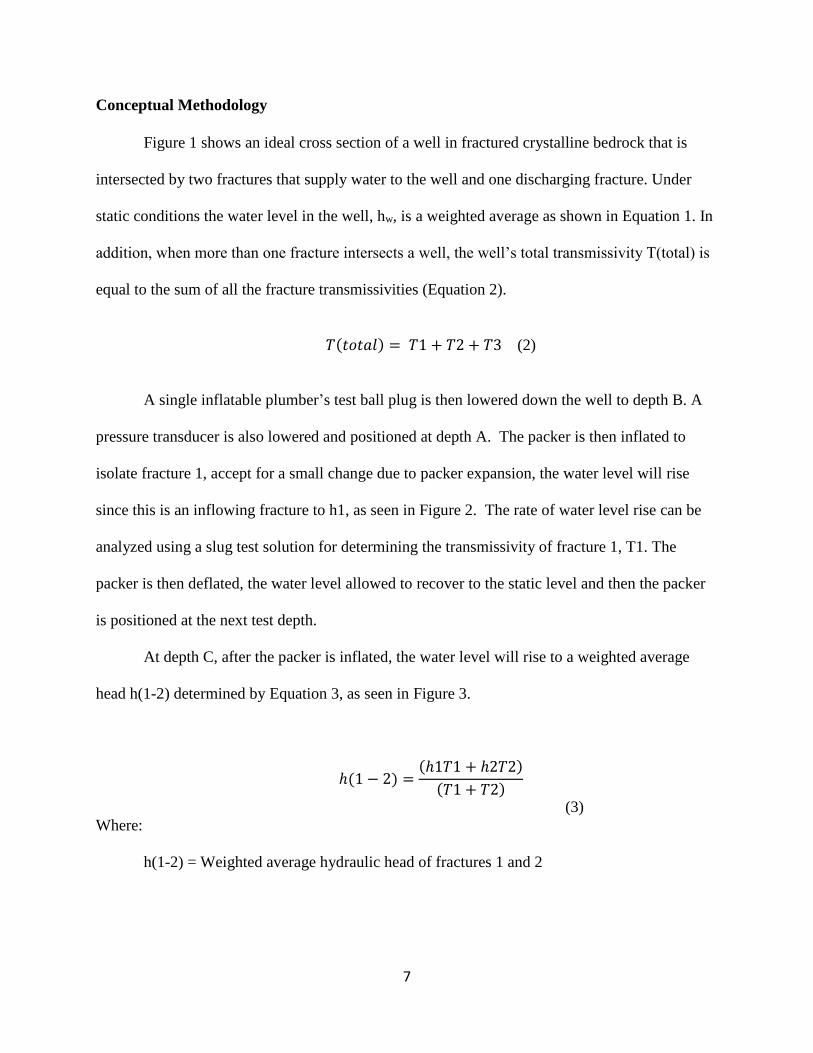
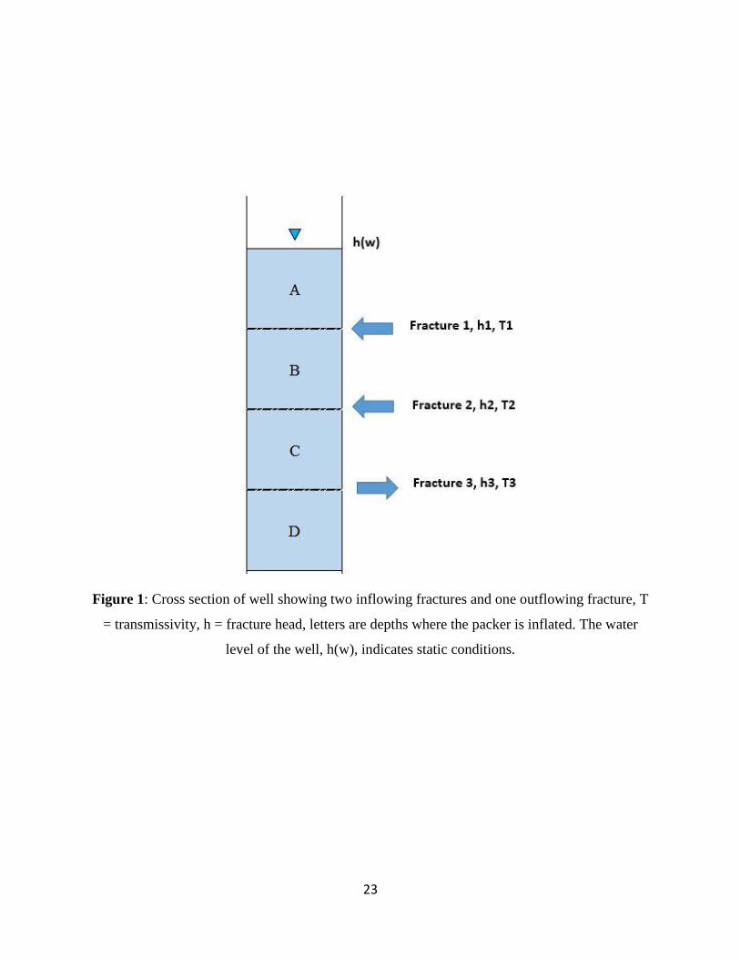
Figure 1 shows an ideal cross section of a well in fractured crystalline bedrock that is

intersected by two fractures that supply water to the well and one discharging fracture. Under

static conditions the water level in the well, hw, is a weighted average as shown in Equation 1. In

addition, when more than one fracture intersects a well, the well’s total transmissivity T(total) is

equal to the sum of all the fracture transmissivities (Equation 2).

𝑇(𝑡𝑜𝑡𝑎𝑙) = 𝑇1 + 𝑇2 + 𝑇3 (2)

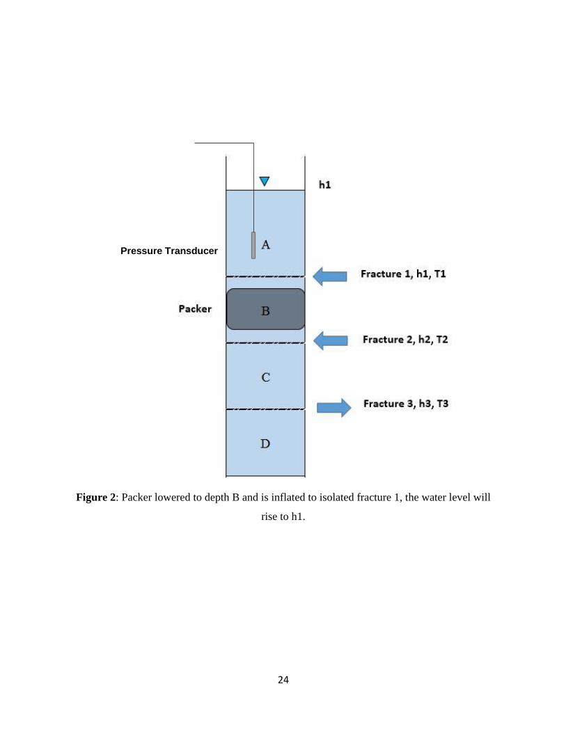
A single inflatable plumber’s test ball plug is then lowered down the well to depth B. A

pressure transducer is also lowered and positioned at depth A. The packer is then inflated to

isolate fracture 1, accept for a small change due to packer expansion, the water level will rise

since this is an inflowing fracture to h1, as seen in Figure 2. The rate of water level rise can be

analyzed using a slug test solution for determining the transmissivity of fracture 1, T1. The

packer is then deflated, the water level allowed to recover to the static level and then the packer

is positioned at the next test depth.

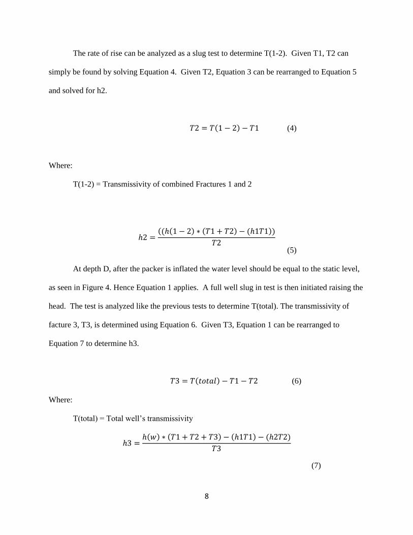
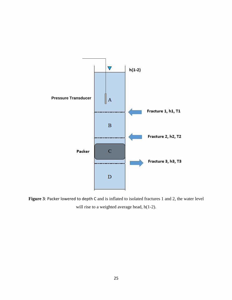
At depth C, after the packer is inflated, the water level will rise to a weighted average

head h(1-2) determined by Equation 3, as seen in Figure 3.

ℎ(1 − 2) =(ℎ1𝑇1 + ℎ2𝑇2)

(𝑇1 + 𝑇2)

(3)

Where:

h(1-2) = Weighted average hydraulic head of fractures 1 and 2

8

The rate of rise can be analyzed as a slug test to determine T(1-2). Given T1, T2 can

simply be found by solving Equation 4. Given T2, Equation 3 can be rearranged to Equation 5

and solved for h2.

𝑇2 = 𝑇(1 − 2) − 𝑇1 (4)

Where:

T(1-2) = Transmissivity of combined Fractures 1 and 2

ℎ2 =((ℎ(1 − 2) ∗ (𝑇1 + 𝑇2) − (ℎ1𝑇1))

𝑇2

(5)

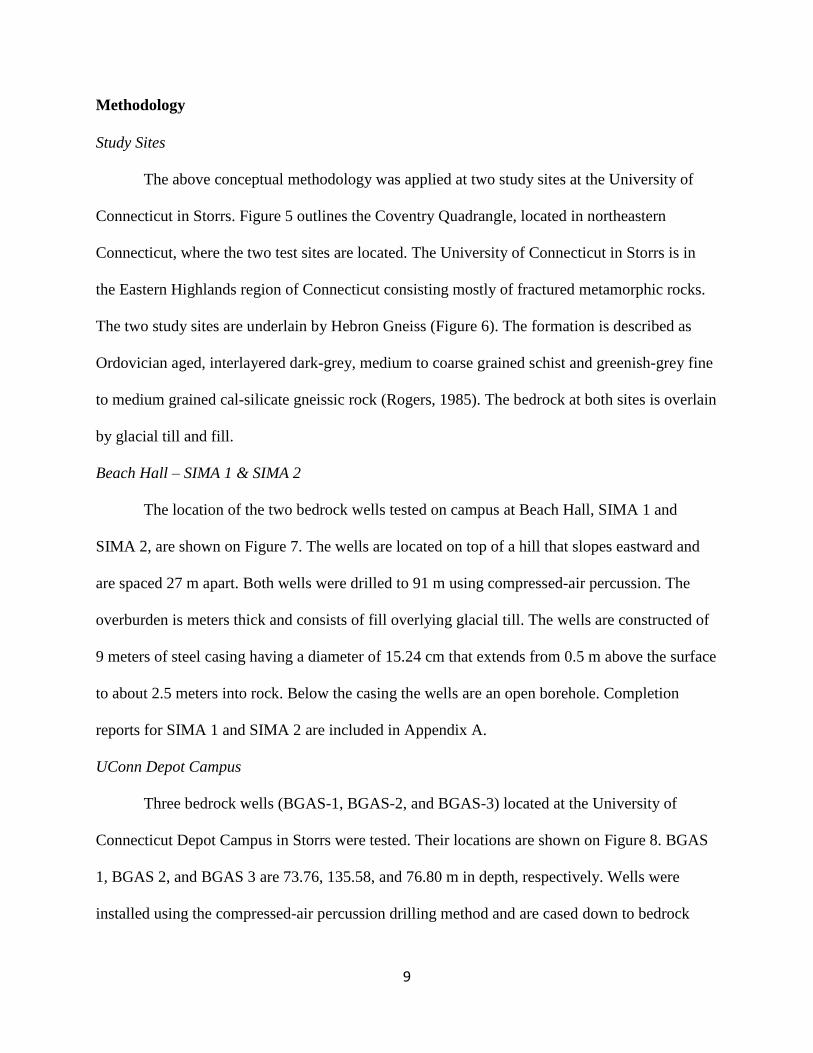
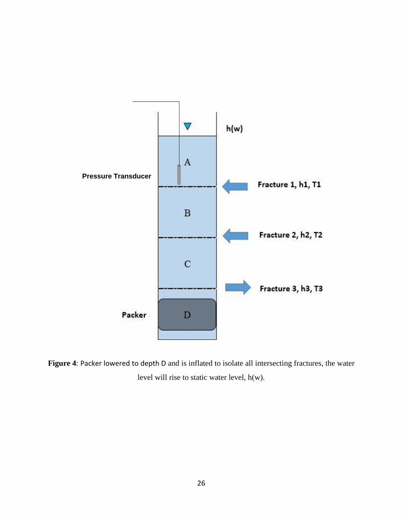
At depth D, after the packer is inflated the water level should be equal to the static level,

as seen in Figure 4. Hence Equation 1 applies. A full well slug in test is then initiated raising the

head. The test is analyzed like the previous tests to determine T(total). The transmissivity of

facture 3, T3, is determined using Equation 6. Given T3, Equation 1 can be rearranged to

Equation 7 to determine h3.

𝑇3 = 𝑇(𝑡𝑜𝑡𝑎𝑙) − 𝑇1 − 𝑇2 (6)

Where:

T(total) = Total well’s transmissivity

ℎ3 =ℎ(𝑤) ∗ (𝑇1 + 𝑇2 + 𝑇3) − (ℎ1𝑇1) − (ℎ2𝑇2)

𝑇3

(7)

9

Methodology

Study Sites

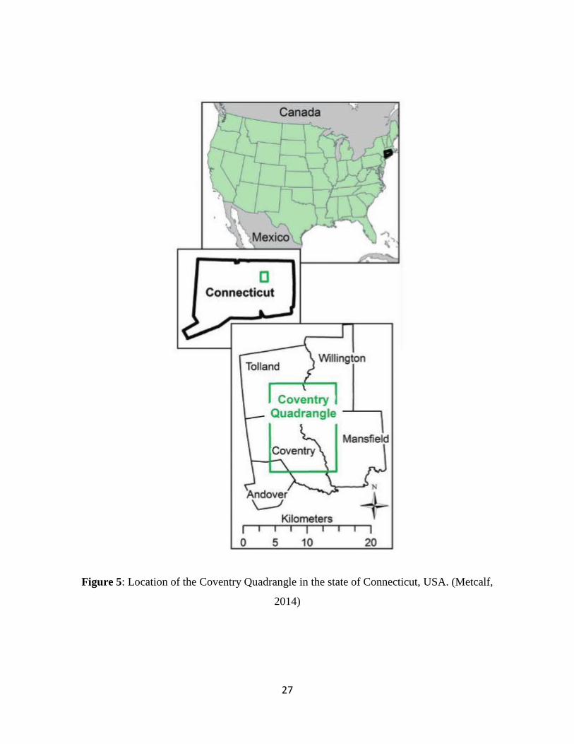
The above conceptual methodology was applied at two study sites at the University of

Connecticut in Storrs. Figure 5 outlines the Coventry Quadrangle, located in northeastern

Connecticut, where the two test sites are located. The University of Connecticut in Storrs is in

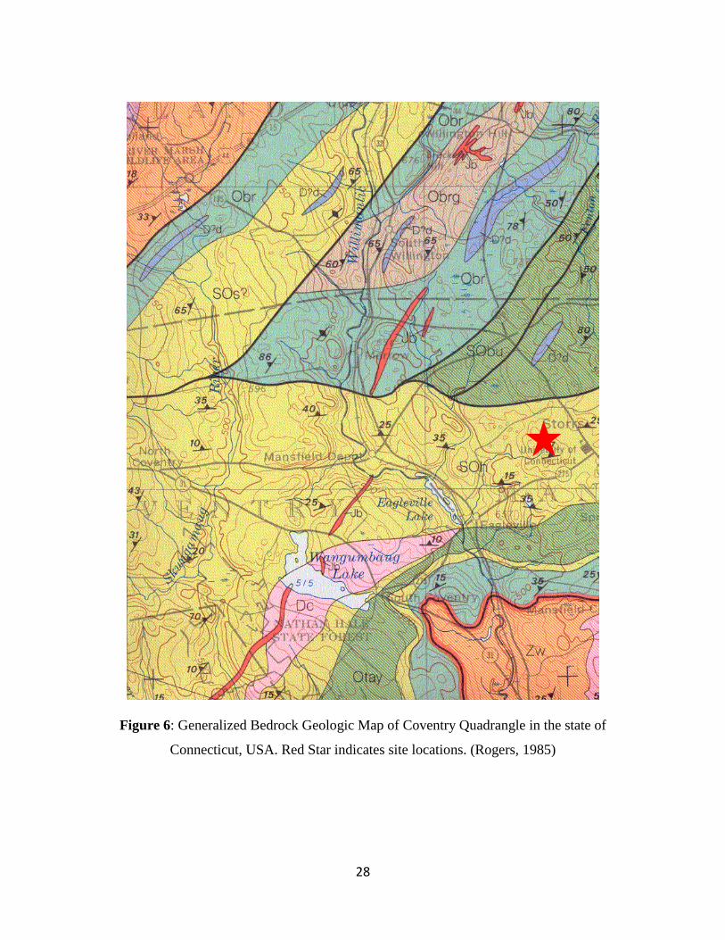
the Eastern Highlands region of Connecticut consisting mostly of fractured metamorphic rocks.

The two study sites are underlain by Hebron Gneiss (Figure 6). The formation is described as

Ordovician aged, interlayered dark-grey, medium to coarse grained schist and greenish-grey fine

to medium grained cal-silicate gneissic rock (Rogers, 1985). The bedrock at both sites is overlain

by glacial till and fill.

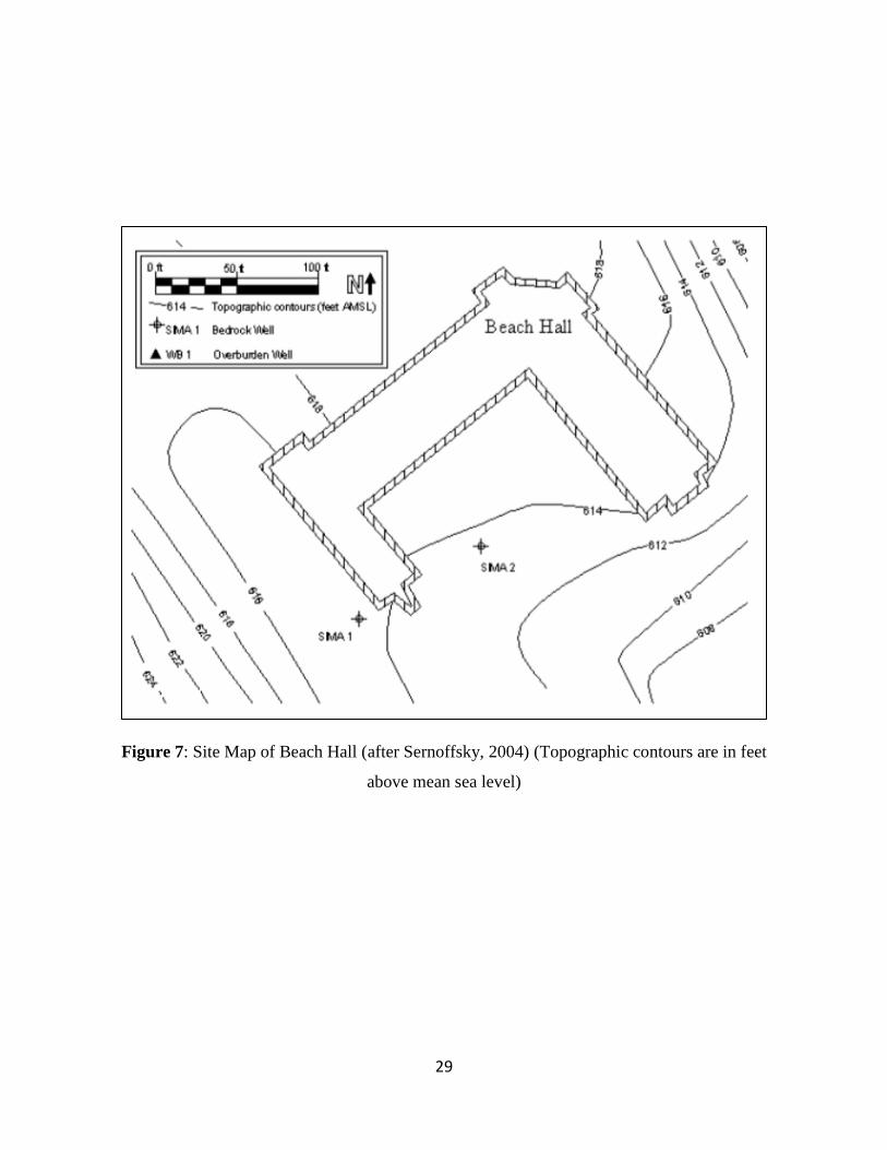
Beach Hall – SIMA 1 & SIMA 2

The location of the two bedrock wells tested on campus at Beach Hall, SIMA 1 and

SIMA 2, are shown on Figure 7. The wells are located on top of a hill that slopes eastward and

are spaced 27 m apart. Both wells were drilled to 91 m using compressed-air percussion. The

overburden is meters thick and consists of fill overlying glacial till. The wells are constructed of

9 meters of steel casing having a diameter of 15.24 cm that extends from 0.5 m above the surface

to about 2.5 meters into rock. Below the casing the wells are an open borehole. Completion

reports for SIMA 1 and SIMA 2 are included in Appendix A.

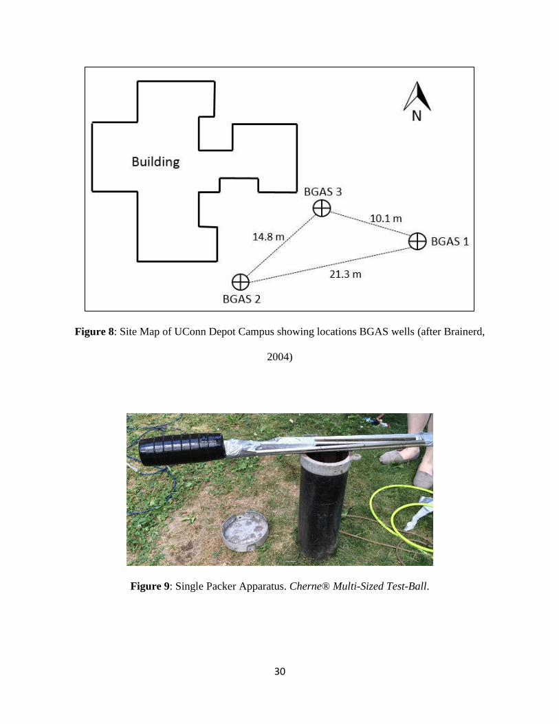
UConn Depot Campus

Three bedrock wells (BGAS-1, BGAS-2, and BGAS-3) located at the University of

Connecticut Depot Campus in Storrs were tested. Their locations are shown on Figure 8. BGAS

1, BGAS 2, and BGAS 3 are 73.76, 135.58, and 76.80 m in depth, respectively. Wells were

installed using the compressed-air percussion drilling method and are cased down to bedrock

10

which lies 4.6 m below the glacial till overburden. The diameter of the well casing is 15.2 cm.

Completion reports for the wells are included in Appendix A.

Field Methods

The results of borehole geophysical investigations (Cagle, 2005; Phillips, 2016) and the

application of the dissolved oxygen alteration method (Chlebica and Robbins, 2013; Vitale,

2016) conducted previously on the test wells were reviewed to determine: (1) the depths of water

transmissive fractures; (2) the direction of borehole flow; and (3) the relative transmissivities.

Discrete fracture intervals of the selected boreholes were isolated using a single Cherne®

Multi-Sized Test-Ball, Part Number: 275048, 4” – 6”, Cost: $140.00 USD (Figure 9). The test

ball was weighted and connected to a pressure line (Flexzilla® Air Hose, Cost: $40.00 USD). A

metal pipe was connected to the pressure line to add weight to the test ball to assist during

descent. At the surface, the line was connected to a regulator of a compressed air tank. An

Instrument Northwest, Inc. (AquiStar®PT2X) or Geoprobe (Model Number: 19345) pressure

transducer was inserted in the well above the upper fracture to measure head changes with time

following packer inflation. Data loggers were programmed to measure and record water levels

every minute.

The packer was slightly inflated to 10 psi to help facilitate lowering it down the borehole.

Once at the required depth, the packer was inflated with compressed air, and left in place until

the water level rose or fell to a steady state head. The pressure required to fully seal the borehole

was calculated using Equation 8.

𝐼𝑛𝑓𝑙𝑎𝑡𝑖𝑜𝑛 𝑃𝑟𝑒𝑠𝑠𝑢𝑟𝑒 = (𝐷𝑝 − 𝐷𝑇𝑊) ∗ 𝐶 + 𝑃𝑝 (8)

Where:

Dp = Depth of packer (ft)

DTW = Depth to water (ft)

11

C = Constant that converts height of water to psi (0.43)

Pp = Packer Inflation Pressure (30 psi)

Periodically the pressure in the packer line was monitored using a high sensitivity gauge

connected to the regulator to verify the packer maintained a seal. Zones of lower transmissivity

require longer periods of time to equilibrate where the packer was sealed in place overnight.

Once the pressure readings reached steady state, the packer was deflated and lowered to another

test interval. After each identified fracture zone was tested, a slug-in test was conducted without

the packer in the well to determine the wellbore’s total transmissivity. This method involves the

addition of a slug of water to the wellbore, raising the head ~1.52 m., and monitoring the fall of

the water level with time.

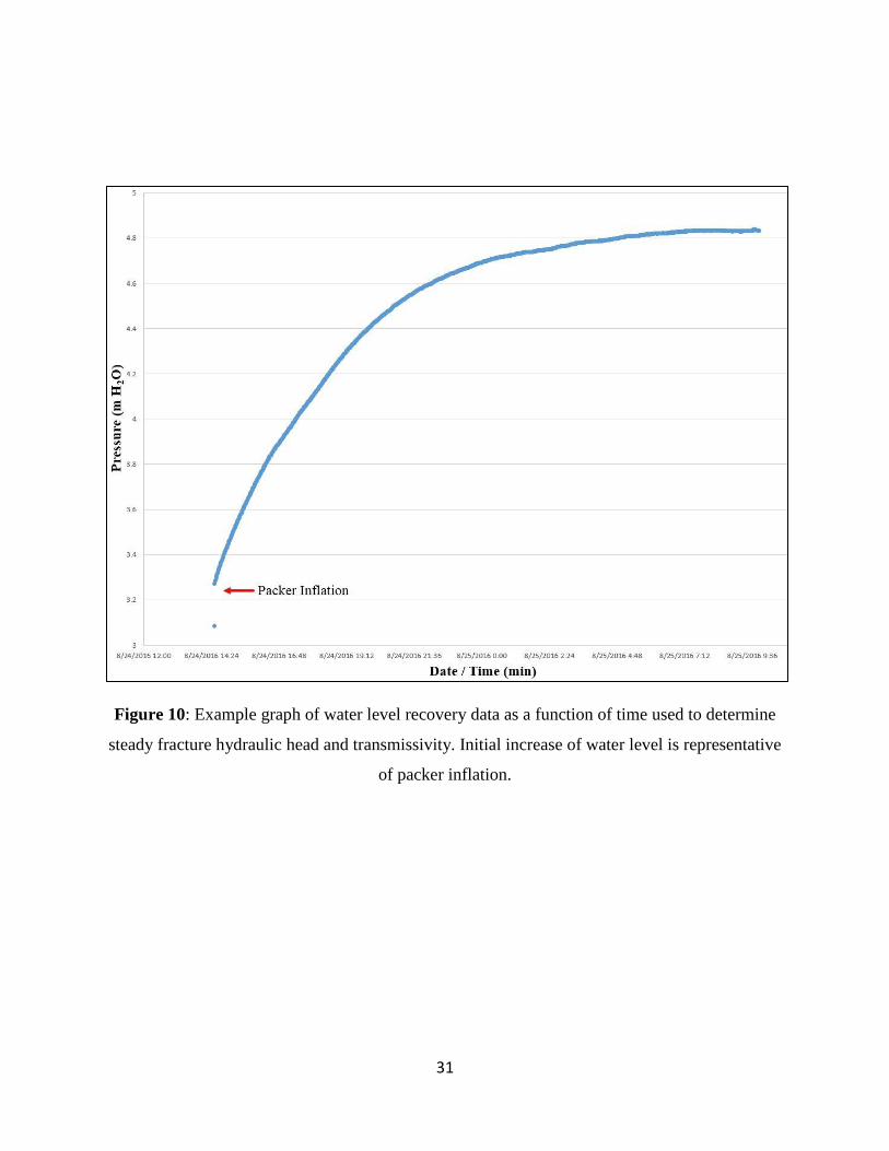
Head and Transmissivity Analysis

The recovery data recorded on the pressure transducer for each test was analyzed to

determine the stable hydraulic head for the depth interval above the packer. This was conducted

by plotting the water pressure vs. time. An example of the water displacement plot is shown in

Figure 10. The water displacement data was subtracted (if pressure rose) or added (if pressure

declined) from the initial pressure reading to obtain the differential head of the zone above the

packer. The steady state differential head was added or subtracted from the well head before

packer inflation to determine the head of the fracture zone. The heads were then processed using

the approach discussed in the conceptual model. Surface elevations that were not previously

recorded were surveyed and measured to the nearest 0.01 foot, referenced to mean sea level.

Depth to water readings were relative to ground surface and were adjusted by subtracting the

casing height above ground surface.

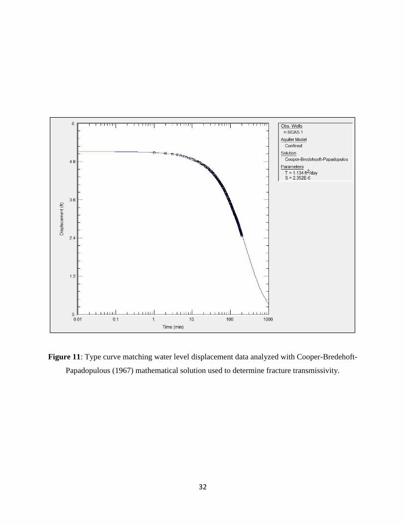
Using the computer program AQTESOLVTM, fracture transmissivity was determined for

each hydraulically active fracture. Using the solution by Cooper-Bredehoeft-Papadopulos (1967)

12

for non-leaky confined aquifers, the analysis involved matching a type-curve to water-level

displacement data for an overdamped slug test (Figure 11).

Results and Discussion

Beach Hall - SIMA 1 & SIMA 2

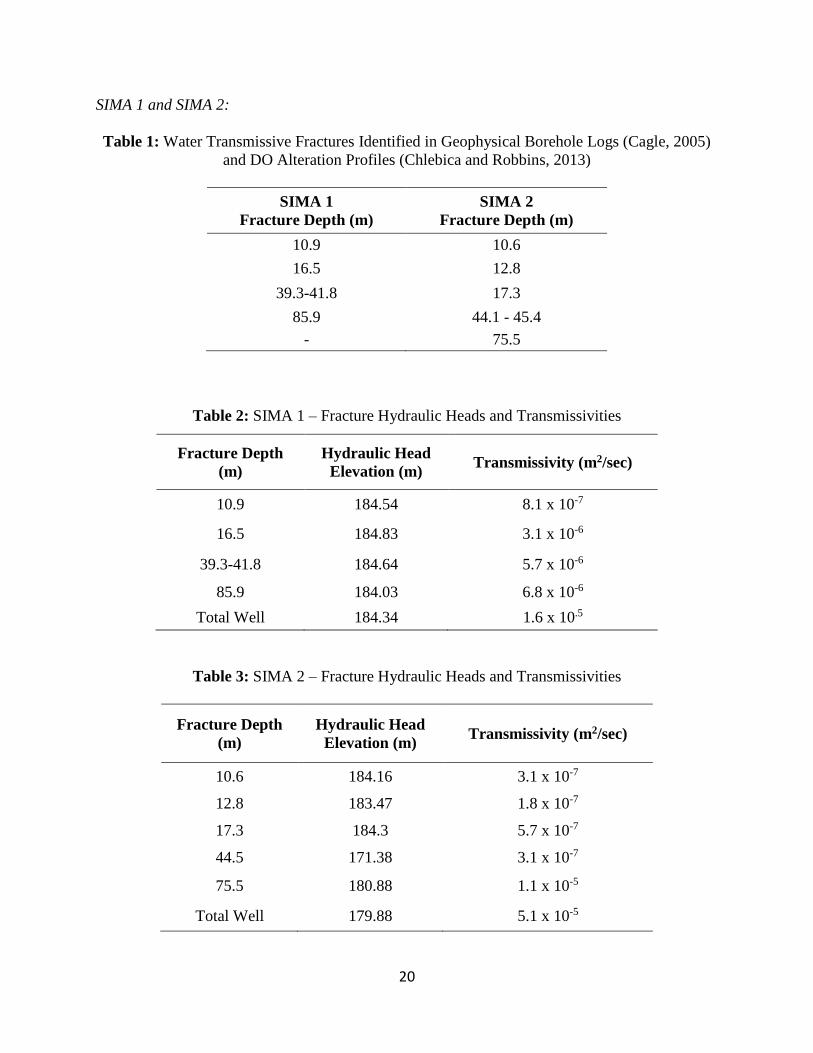
Table 1 lists the water transmissive fractures identified in SIMA 1 and SIMA 2 by

previous studies conducted by Cagle (2005) and Vitale (2017). The televiewer logs were used to

determine the orientation of fractures and foliation. In general, the fractures in SIMA 1 have a

relatively shallow dip angle with a north-northeasterly azimuth or are orientated relatively

horizontal (Cagle, 2005). However, one large fracture located at 39 m has a dip angle of 79

degrees southward and potentially connects to the shallow zone of fractures from 10 – 42 m

outside of the well boring.

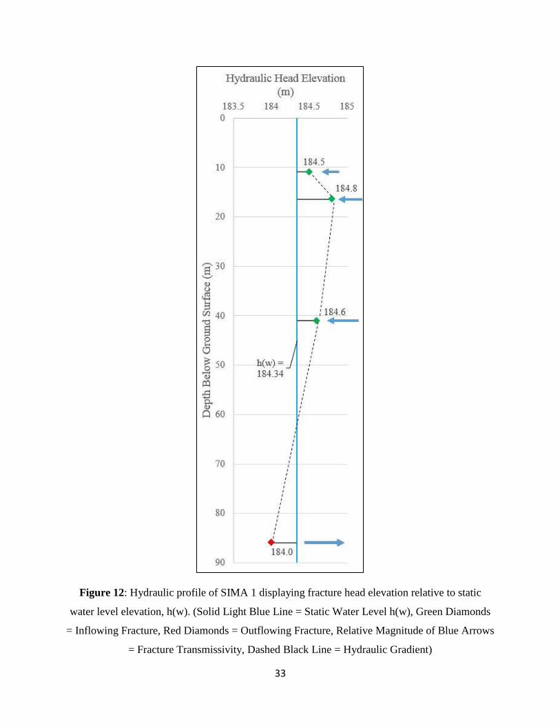
To determine the hydraulic heads and transmissivities of the fractures, the packer was

placed below the fracture depths listed in Table for both SIMA 1 and SIMA 2. Tables 2 and 3 are

the corresponding results of the fracture head and transmissivity determinations in both wells. A

hydraulic profile of SIMA 1, shown in Figure 12, illustrates the fracture head elevations relative

to the static well head elevation. The static well head elevation, hw, of SIMA 1 was 184.34 m.

The three test zones showed increases in head in response to being sealed off from the open

borehole. The vertical orientation of the 41 m fracture likely connects with the 16.5 m and 10.9

m fractures outside the borehole, averaging the fracture heads, which is indicated by the

relatively small changes in head between them. The 10.9 m, 16.5 m, and 41 m fractures have

relative heads of +0.20 m, +0.49 m, and +0.30 m from the static well head (hw) respectively. All

of these were inflowing fractures which is consistent with observations by Cagle (2005) and

13

Chlebica and Robbins (2013). Furthermore, the DO profiles show, under ambient conditions,

water flows down the borehole and out of a fracture near the bottom of the well. The deepest

fracture had the lowest head which was consistent with this flow pattern. The total well’s

transmissivity from a slug test indicated the presence of a highly transmissive fracture below the

tested intervals. The heat pulse flowmeter results from Cagle (2005) verified the presence of a

highly transmissive fracture at a depth of 85 m. Table 2 shows SIMA 1’s fracture transmissivities

increasing with depth, with the most transmissive fracture outflowing at 85 m, largely

influencing the static well head.

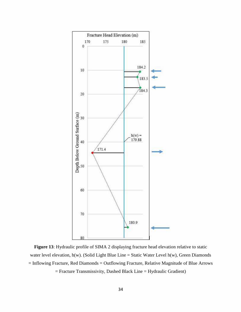
Figure 13 illustrates a hydraulic profile of SIMA 2. Most of the water transmissive

fractures in SIMA 2 have a shallow dip to the north-northwest that parallels the orientation of the

foliation, except for a 45 m deep fracture which has a dip angle of 61 degrees and a south-

southwestward azimuth (Cagle, 2005). The deepest and shallower fractures exhibit heads that

show they were inflowing. The high angle fracture at 45 m was outflowing. Once sealed at 17.3

m, the water level in SIMA 2 rose 4.2 m. In contrast, the 45 m outflowing fracture in SIMA 2

had a relative head of -8.5 m from static hw. The large head differences amongst the fractures in

this well may be related to their dip. The steeply dipping fracture is likely recharged from the

overburden close to the well location but discharges to the overburden further downhill than the

sub-horizontal fractures resulting in a lower head. Given the orientation of the sub-vertical

fractures, they would likely be recharged further uphill than the steeply dipping fracture resulting

in a higher head. The static well head of SIMA 2 had an elevation of 179.88 m, which resulted in

a head difference of 4.46 m from SIMA 1. These wells are known to be hydraulically connected

based on observed drawdown in pumping tests (Cagle, 2005) and studies using the dissolved

oxygen alteration method (Vitale and Robbins, 2015). The latter showed that the fracture at 16.5

14

m in SIMA 1 was connected to the 13.1 m fracture in SIMA 2. The wells are spaced 27 m apart.

Using the hw elevations, the apparent hydraulic gradient between SIMA 1 and SIMA 2 is 0.28 m.

However, the calculated apparent gradient based on the heads in the interconnected fractures was

only 0.05 m, indicating a significant difference in flow rate.

UConn Depot Campus, BGAS 1, BGAS 2, BGAS 3

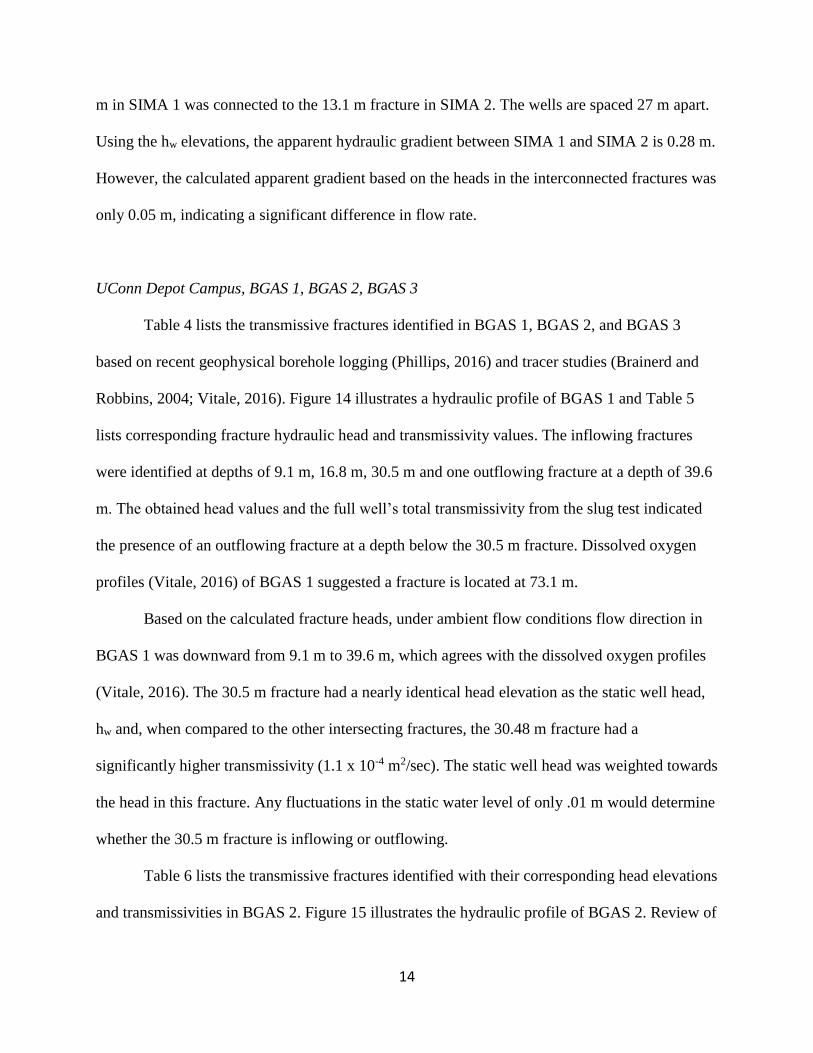
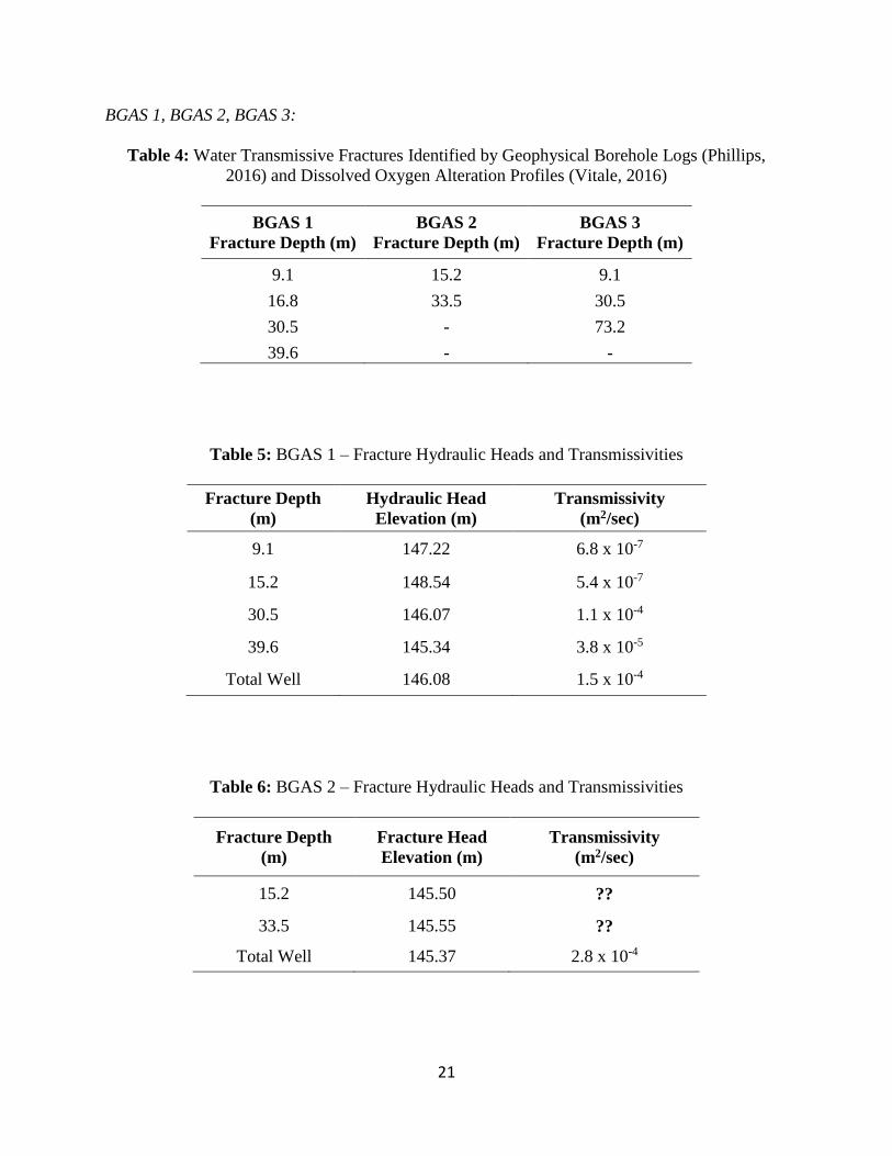
Table 4 lists the transmissive fractures identified in BGAS 1, BGAS 2, and BGAS 3

based on recent geophysical borehole logging (Phillips, 2016) and tracer studies (Brainerd and

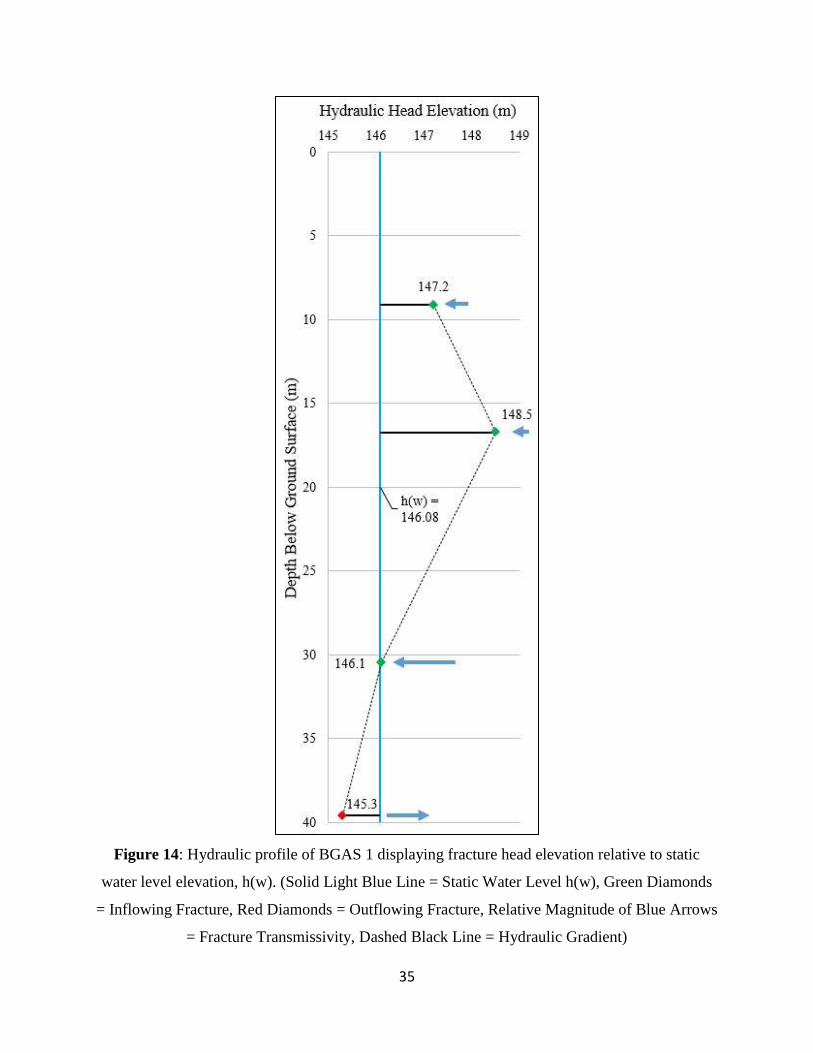
Robbins, 2004; Vitale, 2016). Figure 14 illustrates a hydraulic profile of BGAS 1 and Table 5

lists corresponding fracture hydraulic head and transmissivity values. The inflowing fractures

were identified at depths of 9.1 m, 16.8 m, 30.5 m and one outflowing fracture at a depth of 39.6

m. The obtained head values and the full well’s total transmissivity from the slug test indicated

the presence of an outflowing fracture at a depth below the 30.5 m fracture. Dissolved oxygen

profiles (Vitale, 2016) of BGAS 1 suggested a fracture is located at 73.1 m.

Based on the calculated fracture heads, under ambient flow conditions flow direction in

BGAS 1 was downward from 9.1 m to 39.6 m, which agrees with the dissolved oxygen profiles

(Vitale, 2016). The 30.5 m fracture had a nearly identical head elevation as the static well head,

hw and, when compared to the other intersecting fractures, the 30.48 m fracture had a

significantly higher transmissivity (1.1 x 10-4 m2/sec). The static well head was weighted towards

the head in this fracture. Any fluctuations in the static water level of only .01 m would determine

whether the 30.5 m fracture is inflowing or outflowing.

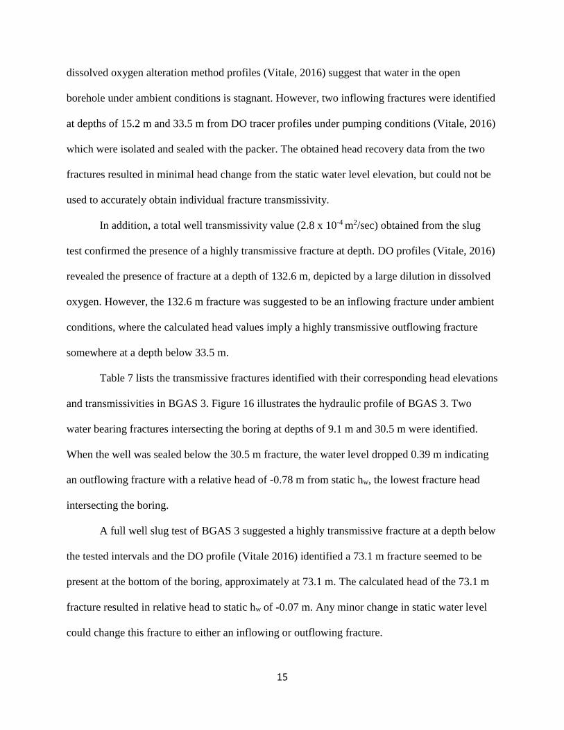
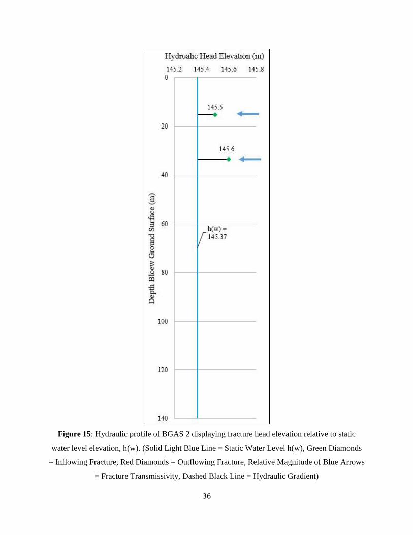
Table 6 lists the transmissive fractures identified with their corresponding head elevations

and transmissivities in BGAS 2. Figure 15 illustrates the hydraulic profile of BGAS 2. Review of

15

dissolved oxygen alteration method profiles (Vitale, 2016) suggest that water in the open

borehole under ambient conditions is stagnant. However, two inflowing fractures were identified

at depths of 15.2 m and 33.5 m from DO tracer profiles under pumping conditions (Vitale, 2016)

which were isolated and sealed with the packer. The obtained head recovery data from the two

fractures resulted in minimal head change from the static water level elevation, but could not be

used to accurately obtain individual fracture transmissivity.

In addition, a total well transmissivity value (2.8 x 10-4 m2/sec) obtained from the slug

test confirmed the presence of a highly transmissive fracture at depth. DO profiles (Vitale, 2016)

revealed the presence of fracture at a depth of 132.6 m, depicted by a large dilution in dissolved

oxygen. However, the 132.6 m fracture was suggested to be an inflowing fracture under ambient

conditions, where the calculated head values imply a highly transmissive outflowing fracture

somewhere at a depth below 33.5 m.

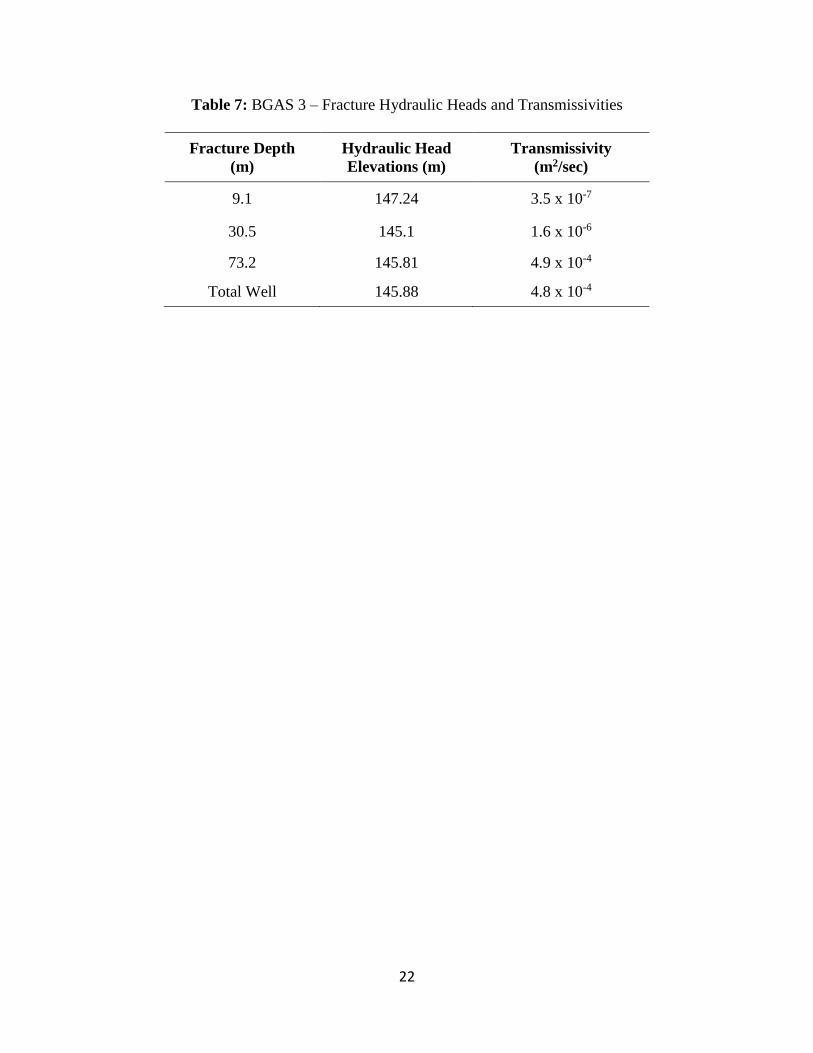
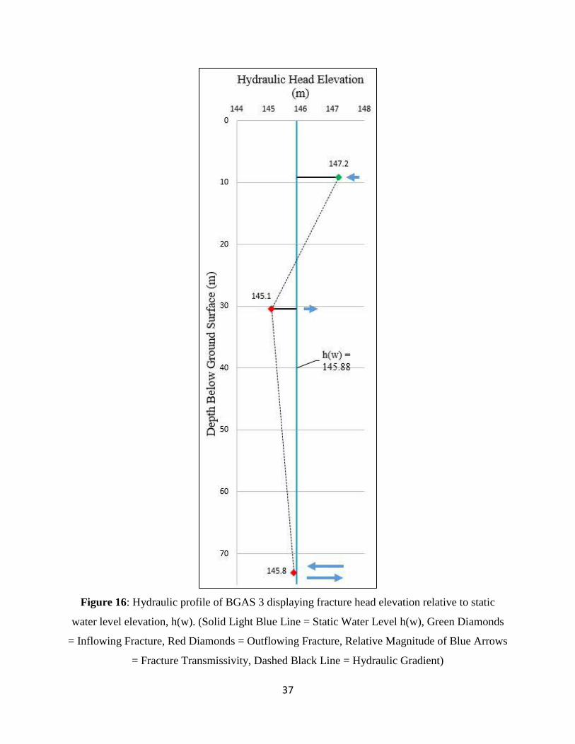
Table 7 lists the transmissive fractures identified with their corresponding head elevations

and transmissivities in BGAS 3. Figure 16 illustrates the hydraulic profile of BGAS 3. Two

water bearing fractures intersecting the boring at depths of 9.1 m and 30.5 m were identified.

When the well was sealed below the 30.5 m fracture, the water level dropped 0.39 m indicating

an outflowing fracture with a relative head of -0.78 m from static hw, the lowest fracture head

intersecting the boring.

A full well slug test of BGAS 3 suggested a highly transmissive fracture at a depth below

the tested intervals and the DO profile (Vitale 2016) identified a 73.1 m fracture seemed to be

present at the bottom of the boring, approximately at 73.1 m. The calculated head of the 73.1 m

fracture resulted in relative head to static hw of -0.07 m. Any minor change in static water level

could change this fracture to either an inflowing or outflowing fracture.

16

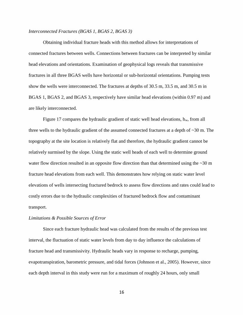
Interconnected Fractures (BGAS 1, BGAS 2, BGAS 3)

Obtaining individual fracture heads with this method allows for interpretations of

connected fractures between wells. Connections between fractures can be interpreted by similar

head elevations and orientations. Examination of geophysical logs reveals that transmissive

fractures in all three BGAS wells have horizontal or sub-horizontal orientations. Pumping tests

show the wells were interconnected. The fractures at depths of 30.5 m, 33.5 m, and 30.5 m in

BGAS 1, BGAS 2, and BGAS 3, respectively have similar head elevations (within 0.97 m) and

are likely interconnected.

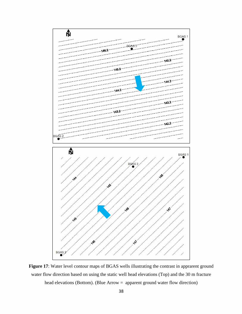
Figure 17 compares the hydraulic gradient of static well head elevations, hw, from all

three wells to the hydraulic gradient of the assumed connected fractures at a depth of ~30 m. The

topography at the site location is relatively flat and therefore, the hydraulic gradient cannot be

relatively surmised by the slope. Using the static well heads of each well to determine ground

water flow direction resulted in an opposite flow direction than that determined using the ~30 m

fracture head elevations from each well. This demonstrates how relying on static water level

elevations of wells intersecting fractured bedrock to assess flow directions and rates could lead to

costly errors due to the hydraulic complexities of fractured bedrock flow and contaminant

transport.

Limitations & Possible Sources of Error

Since each fracture hydraulic head was calculated from the results of the previous test

interval, the fluctuation of static water levels from day to day influence the calculations of

fracture head and transmissivity. Hydraulic heads vary in response to recharge, pumping,

evapotranspiration, barometric pressure, and tidal forces (Johnson et al., 2005). However, since

each depth interval in this study were run for a maximum of roughly 24 hours, only small

17

variations in static water level were observed. By using an average of the static water levels

between testing intervals in calculations this effect can be diminished.

Another potential source of error in this method is packer failure and pressure system

leakage. Deep fractures require additional air hosing for the packer to be inflated at such depths;

therefore, adding more connections could be a source for air leakages. Packer inflations were

checked and water levels monitored during the testing interval to ensure a full seal.

For fractures with head elevations nearly identical to the static well head elevation, the

water level displacement was so minimal and the data would not be used to accurately determine

the transmissivity of the fracture or fracture interval. In order to do so different configurations of

the packer apparatus would be required. In this case, it is suggested to seal off a fracture or

interval of fractures and conduct a slug test while the borehole is sealed at a discrete depth to

obtain a more accurate fracture transmissivity.

Conclusion

This study demonstrates that a cost-effective, simplified single packer fracture

characterization method can be used to confirm the presence and depths of water transmissive

fracture zones and to determine fracture transmissivity and hydraulic head. Used in conjunction

with other methods to locate transmissive fractures, such as the dissolved oxygen alteration

method, the single packer approach can provide a more cost effective means of transmissive

fracture characterization over other available approaches. Although not without its limitations, as

demonstrated here, application of this approach can help eliminate the misleading effects of

using weighted average hydraulic head determinations in open borehole wells in assessing

groundwater flow and solute transport.

18

References

Brainerd, R.J., and G.A. Robbins. 2004. A Tracer Dilution Method for Fracture Characterization

in Bedrock Wells. Ground Water 42, No. 5: 774-780.

Cagle, Matthew B., “Fracture Hydrogeology of Two Wells in Crystalline Bedrock Located in a

Glacial Upland in Connecticut” (2005). Master’s Thesis.

Chlebica, Dariusz, "Modifying Borehole Dissolved Oxygen Levels as a Tool in Deciphering

Fracture Flow Conditions" (2013). Master's Theses.

Chlebica, D.W. and G.A. Robbins. 2013. Altering Dissolved Oxygen to Determine Flow

Conditions in Fractured Bedrock Wells. Groundwater Monitoring and Remediation 33,

no. 4:100-107.

Cooper, H.H., J.D. Bredehoeft and S.S. Papadopulos, 1967. Response of a finite-diameter well to

an instantaneous charge of water, Water Resources Research, vol. 3, no. 1, pp. 263-269.

Haeni, F.P., 2000, Use of Geophysical Tool Box to Characterize Ground-Water Flow in

Fractured-Rock, presented at the EPA Fractured Rock Workshop, Providence, RI,

November 8-9, 2000 (http://water.usgs.gov/ogw/bgas/presentations/epafrcrkcon.pdf).

Johnson, C.D., Kochiss, C.K., and Dawson, C.B., Use of discrete-zone monitoring systems for

hydraulic characterization of a fractured-rock aquifer at the University of Connecticut

landfill, Storrs, Connecticut, 1999 to 2002: U.S. Geological Survey, Water-Resources

Investigations Report 03-4338, 105 p.

Keller, C., Cherry, J.A., Parker, B.L., 2013. New method for continuous transmissivity profiling

in fractured rock. Groundwater. http://dx.doi.org/10.1111/ gwat.12064.

Le Borgne, L., O. Bour, M.S. Riley, P. Gouze, P.A. Pezard, A. Belghoul, G. Lods, R. Le Provost,

R.B. Greswell, P.A. Ellis, E. Isakov, and B.J. Last. 2007. Comparison of alternative

methodologies for identifying and characterizing preferential flow paths in heterogeneous

aquifers. Journal of Hydrology 345, no. 3–4: 134–148.

Metcalf, M. J. and Robbins, G.A., 2014, Evaluating Groundwater Sustainability for Fractured

Crystalline Bedrock. Water Science and Technology: Water Supply, (early pub available

online at doi:10.2166/ws.2013/179)

Neuman, S. P. (2005). Trends, prospects and challenges in quantifying flow and transport

through fractured rocks. Hydrogeology Journal, 13(1), 124-147. DOI: 10.1007/s10040-

004-0397-2

Paillet, F.L. 2000. A field technique for estimating aquifer parameters using flow log data.

Ground Water 38, no. 4: 520–521.

19

Parker, B.L., J.A. Cherry, and S.W. Chapman. 2012. Discrete fracture network approach for

studying contamination in fractured rock. AQUAMundi: Journal of Water Science 60, no.

52: 101–116.

Phillips, Stephanie. Comparison of Flow Logging Methods at a Fractured Rock Site, Storrs,

Connecticut. (2017) University of Connecticut. Masters Thesis.

Quinn P., J.A. Cherry, and B. L. Parker. 2015. Combined use of straddle packer testing and

FLUTe profiling for hydraulic testing in fractured rock boreholes, Journal of Hydrology.,

524, 439–454.

Rogers, J. 1985, Bedrock Geological Map of Connecticut: Connecticut Geological and Natural

History Survey, in cooperation with U.S. Geological Survey, scale 1:125,000.

Sernoffsky R., Robbins G. and Mondazzi R. Use of the In Situ, Inc. MP Troll 9000 to Locate

Fractures Contributing to Ground Water Flow in Bedrock Wells. 2004. U.S. Geological

Survey.

Shapiro, A.M. 2001. Characterizing Ground-Water Chemistry and Hydraulic Properties of

Fractured Rock Aquifers Using the Multifunction Bedrock Aquifer Transportable Testing

Tool (BAT3): U.S. Geological Survey Fact Sheet FS-075- 01, 4 p.

Sokol, Daniel. 1963. Positions and Fluctuations of Water Level in Wells Perforated in More

Than One Aquifer. Journal of Geophysical Research 68, no. 4: 1079-1080.

Vitale, S and Robbins, G. A., 2015, Using Dissolved Oxygen Alteration to Identify Connecting

Transmissive Fractures and Determine Vertical Flow Velocity in Crystalline Bedrock

Wells, GSA Annual Meeting, November 1, Baltimore, Maryland.

Vitale, Sarah A., Advanced Applications of the Dissolved Oxygen Alteration Method (2017).

University of Connecticut. Doctoral Dissertation.

20

SIMA 1 and SIMA 2:

Table 1: Water Transmissive Fractures Identified in Geophysical Borehole Logs (Cagle, 2005)

and DO Alteration Profiles (Chlebica and Robbins, 2013)

SIMA 1

Fracture Depth (m)

SIMA 2

Fracture Depth (m)

10.9 10.6

16.5 12.8

39.3-41.8 17.3

85.9 44.1 - 45.4

- 75.5

Table 2: SIMA 1 – Fracture Hydraulic Heads and Transmissivities

Fracture Depth

(m)

Hydraulic Head

Elevation (m) Transmissivity (m2/sec)

10.9 184.54 8.1 x 10-7

16.5 184.83 3.1 x 10-6

39.3-41.8 184.64 5.7 x 10-6

85.9 184.03 6.8 x 10-6

Total Well 184.34 1.6 x 10.5

Table 3: SIMA 2 – Fracture Hydraulic Heads and Transmissivities

Fracture Depth

(m)

Hydraulic Head

Elevation (m) Transmissivity (m2/sec)

10.6 184.16 3.1 x 10-7

12.8 183.47 1.8 x 10-7

17.3 184.3 5.7 x 10-7

44.5 171.38 3.1 x 10-7

75.5 180.88 1.1 x 10-5

Total Well 179.88 5.1 x 10-5

21

BGAS 1, BGAS 2, BGAS 3:

Table 4: Water Transmissive Fractures Identified by Geophysical Borehole Logs (Phillips,

2016) and Dissolved Oxygen Alteration Profiles (Vitale, 2016)

BGAS 1

Fracture Depth (m)

BGAS 2

Fracture Depth (m)

BGAS 3

Fracture Depth (m)

9.1 15.2 9.1

16.8 33.5 30.5

30.5 - 73.2

39.6 - -

Table 5: BGAS 1 – Fracture Hydraulic Heads and Transmissivities

Fracture Depth

(m)

Hydraulic Head

Elevation (m)

Transmissivity

(m2/sec)

9.1 147.22 6.8 x 10-7

15.2 148.54 5.4 x 10-7

30.5 146.07 1.1 x 10-4

39.6 145.34 3.8 x 10-5

Total Well 146.08 1.5 x 10-4


Fracture Depth

(m)

Fracture Head

Elevation (m)

Transmissivity

(m2/sec)

15.2 145.50 ??

33.5 145.55 ??

Total Well 145.37 2.8 x 10-4

22


Fracture Depth

(m)

Hydraulic Head

Elevations (m)

Transmissivity

(m2/sec)

9.1 147.24 3.5 x 10-7

30.5 145.1 1.6 x 10-6

73.2 145.81 4.9 x 10-4

Total Well 145.88 4.8 x 10-4

23

Figure 1: Cross section of well showing two inflowing fractures and one outflowing fracture, T

= transmissivity, h = fracture head, letters are depths where the packer is inflated. The water

level of the well, h(w), indicates static conditions.

24

Figure 2: Packer lowered to depth B and is inflated to isolated fracture 1, the water level will

rise to h1.

Pressure Transducer

25

Figure 3: Packer lowered to depth C and is inflated to isolated fractures 1 and 2, the water level

will rise to a weighted average head, h(1-2).

Pressure Transducer

26

Figure 4: Packer lowered to depth D and is inflated to isolate all intersecting fractures, the water

level will rise to static water level, h(w).

Pressure Transducer

27

Figure 5: Location of the Coventry Quadrangle in the state of Connecticut, USA. (Metcalf,

2014)

28

Figure 6: Generalized Bedrock Geologic Map of Coventry Quadrangle in the state of

Connecticut, USA. Red Star indicates site locations. (Rogers, 1985)

29

Figure 7: Site Map of Beach Hall (after Sernoffsky, 2004) (Topographic contours are in feet

above mean sea level)

30

Figure 8: Site Map of UConn Depot Campus showing locations BGAS wells (after Brainerd,

2004)

Figure 9: Single Packer Apparatus. Cherne® Multi-Sized Test-Ball.

31

Figure 10: Example graph of water level recovery data as a function of time used to determine

steady fracture hydraulic head and transmissivity. Initial increase of water level is representative

of packer inflation.

32

Figure 11: Type curve matching water level displacement data analyzed with Cooper-Bredehoft-

Papadopulous (1967) mathematical solution used to determine fracture transmissivity.

33

Figure 12: Hydraulic profile of SIMA 1 displaying fracture head elevation relative to static

water level elevation, h(w). (Solid Light Blue Line = Static Water Level h(w), Green Diamonds

= Inflowing Fracture, Red Diamonds = Outflowing Fracture, Relative Magnitude of Blue Arrows

= Fracture Transmissivity, Dashed Black Line = Hydraulic Gradient)

34

Figure 13: Hydraulic profile of SIMA 2 displaying fracture head elevation relative to static




35

Figure 14: Hydraulic profile of BGAS 1 displaying fracture head elevation relative to static




36





37





38

Figure 17: Water level contour maps of BGAS wells illustrating the contrast in apprarent ground

water flow direction based on using the static well head elevations (Top) and the 30 m fracture

head elevations (Bottom). (Blue Arrow = apparent ground water flow direction)

Documents

A Single Packer Method for Characterizing Water