A SIMPLE PROBABILISTIC APPROACH TO CLASSIFICATION AND ROUTING

Louise Guthrie I

James Leistensnider

Lockheed Martin Corporation

P.O. Box 8048 Philadelphia, PA 19101

guthrie,leistens@mds.lmco.com

1. ABSTRACT

Several classiiiCation and routing methods were im­plemented and compared. The experiments used FBIS documents from four categories, and the measures used were the tf.idf and Cosine similarity measures, and a maximum likelihood estimate based on assuming a Multinomial Distribution for the various topics (popula­tions). In addition, the SMART program was run with 'lnc.ltc' weighting and compared to the others.

Decisions for both our classifiCation scheme (docu­ments are put into any number of disjoint categories) and our routing scheme (documents are assigned a 'score' and ranked relative to each category) are based on the highest probability for correct classification or routing. All of the techniques described here are fully automatic, and use a training set of relevant documents to produce lists of distinguishing terms and weights. All methods (ours and the ones we compared to) gave excel­lent results for the classification task, while the one based on the Multinomial Distribution produced the best results on the routing task.

2. INTRODUCTION

One of the goals of the TIPSTER Phase ll Extraction Project [Contract Number 94-F133200-000] has been to integrate extraction and detection technologies. In this paper we extend previous work (Guthrie, et al) [1] on classifying texts into categories, and develop a meth­odology based on the classification technique for rout­ing documents.

By classifying and routing texts into categories we mean to include a variety of applications; categorizing texts by topic, by the language the text is written in, or by relevance to a specified task. The techniques used here are not language specific and can be applied to any language or domain.

167

2.1. The Intuitive Model

The mathematical model we use in this paper for­malizes the intuitive notion that humans can identify the topic of an unfamiliar article based on the occurrence of topic specific words and phrases. Note that most people can tell that the first passage below is about music, even though the word 'music' is not in the passage. Similarly, most people can tell that the second passage is from a sports article, even though the word 'sport' is never mentioned.

"Before the release of his last studio album, 1993's 'Ten Summoner's Tales', Sting commented that he could no longer put his whole heart into his work; it left him feeling too vulnerable. Not surprisingly, that disc was well-crafted, but a bit void of feeling--unfortunate, considering the wondrous synergy of heart and craft on Sting's masterwork, 1987's 'Nothing Like the Sun'. Sadly, 'Mercury Falling' makes 'Ten Summoner's Tales' seem brilliant by comparison. It's as if Sting only made it because he looked at his calendar one day and real­ized, by golly, that it was time to make another record. Easily the worst album of what has until now been a re­markably successful career, the disc is aptly named: the temperature never seems to rise on this turgid effort." [2]

"Walter McCarty scored 24 points and Antoine Walker had 14 and nine rebounds as Kentucky pulled away in the second half to beat upstart San Jose State, 110-72, in the first round of the Midwest Regional in Dallas.

The Wildcats (28-3), who are seeking their first na­tional championship since 1978, will meet the winner of the Wisconsin-Green Bay-Virginia Tech game on Satur­day at Reunion Arena.

San Jose State, which was making its first NCM Tournament appearance, gave Kentucky all it could handle in the first half, tying the game at 37-37 with 2:50 to play. The Wildcats then closed out the first half

Report Documentation Page Form ApprovedOMB No. 0704-0188

Public reporting burden for the collection of information is estimated to average 1 hour per response, including the time for reviewing instructions, searching existing data sources, gathering andmaintaining the data needed, and completing and reviewing the collection of information. Send comments regarding this burden estimate or any other aspect of this collection of information,including suggestions for reducing this burden, to Washington Headquarters Services, Directorate for Information Operations and Reports, 1215 Jefferson Davis Highway, Suite 1204, ArlingtonVA 22202-4302. Respondents should be aware that notwithstanding any other provision of law, no person shall be subject to a penalty for failing to comply with a collection of information if itdoes not display a currently valid OMB control number.

1. REPORT DATE MAY 1996 2. REPORT TYPE

3. DATES COVERED 00-00-1996 to 00-00-1996

4. TITLE AND SUBTITLE A Simple Probabilistic Approach to Classification and Routing

5a. CONTRACT NUMBER

5b. GRANT NUMBER

5c. PROGRAM ELEMENT NUMBER

6. AUTHOR(S) 5d. PROJECT NUMBER

5e. TASK NUMBER

5f. WORK UNIT NUMBER

7. PERFORMING ORGANIZATION NAME(S) AND ADDRESS(ES) Lockheed Martin Corporation,P.O. Box 8048,Philadelphia,PA,19101

8. PERFORMING ORGANIZATIONREPORT NUMBER

9. SPONSORING/MONITORING AGENCY NAME(S) AND ADDRESS(ES) 10. SPONSOR/MONITOR’S ACRONYM(S)

11. SPONSOR/MONITOR’S REPORT NUMBER(S)

12. DISTRIBUTION/AVAILABILITY STATEMENT Approved for public release; distribution unlimited

13. SUPPLEMENTARY NOTES TIPSTER TEXT PROGRAM PHASE II: Proceedings of a Workshop held at Vienna, Virginia, May 6-8,1996. Sponsored by the Defense Advanced Research Projects Agency.

14. ABSTRACT Several classification and routing methods were implemented and compared. The experiments used FBISdocuments from four categories, and the measures used were the ff.idf and Cosine similarity measures, anda maximum likelihood estimate based on ass~lming a Multinomial Distribution for the various topics(populations). In addition, the SMART program was run with ’lnc.ltc’ weighting and compared to theothers. Decisions for both our classification scheme (documents are put into any number of disjointcategories) and our routing scheme (documents are assigned a ’score’ and ranked relative to eachcategory) are based on the highest probability for correct classification or routing. All of the techniquesdescribed here are fully automatic, and use a training set of relevant documents to produce lists ofdistin~i~hin?? terms and weights. All methods (ours and the ones we compared to) gave excellent resultsfor the classification task, while the one based on the Multinomial Distribution produced the best results onthe routing task.

15. SUBJECT TERMS

16. SECURITY CLASSIFICATION OF: 17. LIMITATION OF ABSTRACT Same as

Report (SAR)

18. NUMBEROF PAGES

11

19a. NAME OFRESPONSIBLE PERSON

a. REPORT unclassified

b. ABSTRACT unclassified

c. THIS PAGE unclassified

Standard Form 298 (Rev. 8-98) Prescribed by ANSI Std Z39-18

with an 11-4 run to build a 47-41 advantage at the inter­mission.

Olivier Saint-Jean finished with 18 points and seven rebounds for the Spartans (13-17), who were one of two teams in the NCM Tournament with a losing record." [3]

The music passage has many music related words such as 'studio', 'album', 'disc', and 'record', and the sports passage has many sports related words such as 'scored', 'beat', 'championship', 'game', and 're­bounds'. Any of these words taken singly would not necessarily give a strong indication about the passage topic, but taken together they can predict with a high de­gree of certainty the topic of the passage.

2.2. The Mathematical Model

The mathematical model used here is to represent each category as a multinomial distribution. Parameters are estimated from the frequency of certain sets of words and phrases (the 'distinguishing word sets') found in the training collections.

Previous results (Guthrie et all994) indicate that the simple statistical technique of the maximum likelihood ratio test would, under certain conditions, give rise to an excellent classification scheme for documents. Pre­vious theoretical results were verified using two classes of documents, and excellent recall and precision scores were achieved for distinguishing topics (previous tests were conducted in both Japanese and English). In this paper we both extend the classification scheme to in­clude any number of topics and modify the scheme to also perform routing.

In modeling a class of text. our technique requires that we identify a set of key concepts, or distinguishing words and phrases. The intuition is given in the example above, but in this work we want to automate the process of choosing word sets in a way that results in sets of 'dis­tinguishing concepts'.

In (Guthrie et al1994), it was shown that if the prob­abilities of the distinguishing word sets in each of the classes is known, we can predict the probability of cor­rect classification. Our goal eventually is to define an algorithm for choosing 'distinguishing word sets' in an optimal way; i.e. a way that will maximize the probabil­ity of correct classification. The method we use now (described in section 4.1.) is empirical, but allows us to guarantee excellent classification results.

2.3. Common Approaches

Schemes for classification and routing all tend to follow a particular paradigm:

1. Represent each class (or topic or profile or bucket) as a numerical object.

2. Represent each new document that arrives as a numerical object.

3. Measure the 'similarity' between the new document and each of the classes.

4. For Oassification - Place the new document in the category corresponding to the class (or bucket or profile) to which it is most similar. For Routing - Rank the document in the class using some function of the similarity measure.

Although many similarity measures have been stu­died, two of them seem to have gained popularity in the recent literature: the Cosine and tf.idf measures. The Cosine measure is used when a document is represented as a multi-dimensional vector. and a document is de­fined as more similar to Class 1 than Class 2 if its corre­sponding vector is closer to that of Oass 1 than to that of Class 2. In tf.idf a document is more similar to Class 1 than Class 2 if more terms match the Oass 1 terms than do the Class 2 terms. In our work a document is more similar to Oass 1 than Oass 2 if the probability ·Of it be­longing to Oass 1 is greater than the probability of it be­longing to Oass 2.

In choosing a representation of a class or a represen­tation of a document, much of the current research in classification and routing is focused on choosing the best set of terms (in our case. we call them Distinguish­ing Terms) to represent it. Many systems start with prevalent but not common (so that words such as 'the' and 'to' are not used) words and phrases in the class training set. The training set may be as small as the ini­tial query which defined the class or as large as all of the documents which are available which are deemed to be relevant to the class. If this set of terms is too small, feedback is generally employed in which the full corpus of documents to be classified and routed is compared to the set, prevalent words and phrases from highly ranked retrieved documents are added to the set. and the full corpus is run again against the larger set of terms.

168

2.4. Probabilistic Classification Approach Using Multinomial Distribution

A probabilistic method for classification was pro­posed by Guthrie and Walker [1], which assumed each class was distributed by the multinomial distribution. Elementary statistics tells us that a maximum likelihood ratio test is the best way to calculate the probability that a set of outcomes was produced by a given input. In the example below, we assume a multinomial distribution for our dice and fmd the largest conditional probability of getting a certain output given a certain input. For ex-

ample, consider the set of outcomes produced by rolling one of two single six-sided dice. One of the dice is fair and one is loaded to be more likely to give a '6' out­come. Let us assign the expected probabilities for the outcomes for each of the two dice.

Die

Fair Loaded

Outcome 1 2 3 4 5 6

Probability

1~ 1~ 1~ 1~ 1~ 1~ 1/10 1/10 1/10 1/10 1/10 1{1.

Table 2.3-1. Expected Probabilities

Now let us defme three sets of outputs.

Outcome

1 2 3 4 5 6

Output Count

set 1 5 4 4 6 5 4 set2 2 3 1 2 4 10 set 3 3 4 2 5 4 8

Table 2.3-2. Outputs

Using the multinomial distribution, we may calcu­late which is the more likely die to have produced each of the outputs. The multinomial equation is shown be­low, for the case of 6 possible outcomes.

Using the probabilities assigned to each die for PI through P6· and the number of times each outcome oc­curred for n1 through fi6, and the total number of out­comes for n, the following probabilities of producing each output given that a particular die was used are cal­culated.

Output Fair Die Loaded Die set 1 3.46 X 10-4 1.33 X 10-7 set 2 4.09 X 10-6 5.25 X 10-4 set 3 7.07 x lo--s 4.71 x 1o--s

Table 2.3-3. Probability of Output

The most likely die to produce each output is the one with the maximum probability. We can see that these probabilities are an excellent measure for determining which of the dice was more likely to be used to generate each of the sets of outcomes. Set 1, which has a fairly uniform distribution, is much more likely to have been created with the fair die than the loaded one. Set 2, which has nearly half of the outcomes as '6', is much more likely to have been created with the loaded die

169

than the fair one. Set 3 does not have an obvious dis­tribution. It has more '6' outcomes than would be ex­pected with the fair die. but not as many as would be ex­pected with the loaded die. As it turns out, it is just slightly more likely that the fair die was used to generate set3.

Applying this approach to the document classifica­tion problem. we may defme the outcomes to be the sets of Distinguish Terms which defme the classes. The ex­pected probabilities are then the sum of the frequencies of the Distinguishing Terms in each of the classes di­vided by the training set lengths. The outputs are the counts of how many of the Distinguishing Terms from each class are evident in a document. Since to create a multinomial distribution all possible outcomes must be accounted for, an additional count is kept of all of the words in a document are not members of any of the Dis­tinguishing Term sets. The expected probability for this set of words is 1.0 minus the sum of the probabilities of all of the Distinguishing Terms in the training set.

2.5. Probabilistic Routing Approach Us­ing Multinomial Distribution

Expanding this approach to the routing problem, we want to fmd the most likely class given the probabilities of the outputs. This can be calculated with Bayes' Theo­rem, using the assumption that all classes have equally likely occurrences.

P(clasSj I output) = P(output I classJ

P(output)

Continuing the example with the fair and the loaded die, the sets are assigned probabilities that they belong to each of the classes given the fact that they have a cer­tain set of outcomes. This would result in the following probabilities.

Output set 1 set2 set 3

Fair Die 0.999616 0.007730 0.600170

Loaded Die 0.000384 0.992270 0.388830

Table 2.3-4. Probability of Oass

Sorting these probabilities. we get the expected re­sults; set 1 is the output most likely to have been created with the fair die and set 2 the least. and set 2 is the output most likely to have been created with the loaded die and set 1 the least.

Comparing these routing results to the classification results, the question may be raised why the probability that a set is from a class needs to be calculated. Ranking with the probability of getting the outputs (Table 2.3-3) would have given the same ranking. But now consider the case in which set 3 was ten times larger, as shown in the table below.

Outcome

1 2 3 4 5 6

Output Count

set 1 5 4 4 6 5 4 set2 2 3 1 2 4 10 set 3 30 40 20 so 40 80

Table 2.3-5. Outputs

Our expectation is still that set 3 should be ranked in the middle, between sets 1 and 2 for each die. Calculat­ing the probabilities of getting these outputs, we get the following table.

Output

set 1 set2 set 3

Fair Die Loaded Die

3.46 X 10-4 1.33 X Ht-7

4.09 X 1Q-6 5.25 X IQ-4 1.96 X lQ-16 3.39 X IQ-18

Table 2.3-6. Probability of Output

Using these probabilities directly for ranking would place set 3 on the bottom of each list, which does not agree with intuition. Note that this problem is the same problem that document retrieval systems have with doc­uments of varying lengths; longer documents are ranked lower than they should be. But now we take the second step of calculating the probability that an output is in a class.

Output

set 1 set2 set 3

Fair Die

0.999616 0.007730 0.982998

Loaded Die

0.000384 0.992270 0.017002

Table 2.3-7. Probability of Class

We can see that now the rankings are as we expect; set 1 is the output most likely to have been created with the fair die and set 2 the least, and set 2 is the output most likely to have been created with the loaded die and set 1 the least. So using this multinomial distribution to rank documents is less likely to be adversely affected by varying document lengths.

3. APPROACH

Below is a description of the different approaches implemented for calculating the match between a docu­ment and a class profile. The class scores are then compared to each other to determine the classification and routing results.

3.1. Class Scoring Techniques tf.idf

The weight associated with each term in the training set is the log of the number of classes divided by the number of classes which contain the term.

The class score is calculated by the following equa­tion [2]. This equation has been modified from the ref­erence by dividing by the sum over the class of the term weights. to normalize the results when Distinguishing Term sets are used which have different lengths.

I count (weight x ( _1.

2 + _1.

2 ----)) max. count

document

score= -------------------------

Cosine

I weight

class

The weight associated with each term in the training set is calculated by the following equation [1].

[

number of classes weight= log number of classes with term

170

The class score is calculated by the following equa­tion [1].

L (weightxlog(count+ 1))

document

L (weight)2 x L (log(count + 1))2

class document

Multinomial Distribution

A number of weights are associated with each term in the training set. A weight is calculated for each of the classes for each term, and the weight is the probability of the term occurrence in the class. This is approxi­mated by taking the frequency of the term occurrence in the training set divided by the size of the training set. The weights for all of the Distinguishing Terms in a set are combined into a single value, called the set weight. An additional weight is calculated, which is necessary for the multinomial distribution. This is the probability that a term is not a Distinguishing Term, and is calcu­lated as 1.0 minus the sum of the probabilities of all of the Distinguishing Terms in the training set. Since the class scores calculated with this approach are exceed­ingly small, the log of the probability equation is used to avoid computational difficulties.

The class score is calculated by the following equa­tion [3].

score =~og ( n! l nd ... D.J.! fik+l!

n = number of words in document k = number of classes ni = number of terms from the ith set fik+l =number of words which do not match any set

For routing, the score is the probability for each class calculated given the words in the document. This is done with the following equation for each class.

score routing score =

sum of all scores

SMART

The SMAIIT program independently calculates the scores for the Distinguishing Terms and for the docu­ment based upon the word frequencies in the entire collection available for classifiCation and routing, and takes the score as the sum of the products of the Distin­guishing Term and document weights. A variety of weighting schemes are possible, and a common one is called 'lnc.ltc'. The weight associated with each term in the Distinguishing Term set is calculated by the fol­lowing equation [6].

log [YJ weight= -;:=====-

Jr_log[YJ class

k = number of classes m = number of classes with term

The class score is calculated by the following equa­tion [6].

score= I document

(log (count) + 1)

I (log (count) + 1)

class

x weight

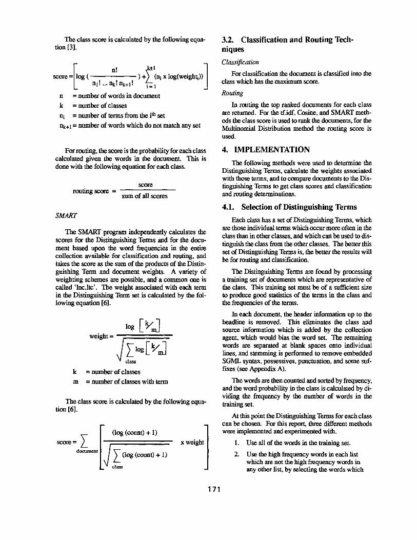
171

3.2. Classification and Routing Tech­niques

Classification

For classification the document is classified into the class which has the maximum score.

Routing

In routing the top ranked documents for each class are returned. For the tf.idf, Cosine, and SMART meth­ods the class score is used to rank the documents, for the Multinomial Distribution method the routing score is used.

4. IMPLEMENTATION

The following methods were used to determine the Distinguishing Terms, calculate the weights associated with those terms, and to compare documents to the Dis­tinguishing Terms to get class scores and classification and routing determinations.

4.1. Selection of Distinguishing Terms

Each class has a set of Distinguishing Terms, which are those individual terms which occur more often in the class than in other classes, and which can be used to dis­tinguish the class from the other classes. The better this set of Distinguishing Terms is, the better the results will be for routing and classification.

The Distinguishing Terms are found by processing a training set of documents which are representative of the class. This training set must be of a suffiCient size to produce good statistics of the terms in the class and the frequencies of the terms.

In each document, the header information up to the headline is removed. This eliminates the class and source information which is added by the collection agent. which would bias the word set. The remaining words are separated at blank spaces onto individual lines, and stemming is petformed to remove embedded SGML syntax, possessives, punctuation. and some suf­fixes (see Appendix A).

The words are then counted and sorted by frequency. and the word probability in the class is calculated by di­viding the frequency by the number of words in the training set.

At this point the Distinguishing Terms for each class can be chosen. For this report, three different methods were implemented and experimented with.

1. Use all of the words in the training set.

2. Use the high frequency words in each list which are not the high frequency words in any other list, by selecting the words which

are in the highest so many on the list and not in the highest so many on any other list.

3. Use the high frequency words in each list which occur with low frequency on all of the other lists, by selecting only the words which occur more often in one list than in all other lists combined, until enough words have been chosen.

4.2. Calculation of Term Weights

Each of the selection methods requires a weight to be calculated for each Distinguishing Term. The tf.idf and Cosine methods all calculate the weight using the number of classes which contain the term, while the Multinomial Distribution method calculates the weight using the term probabilities.

tfidf

[ number of classes J

weight = log number of classes with term

Cosine

[ number of classes

weight = log number of classes with term

Multinomial Distribution

Each term has a weight for each class.

weightc1ass i = probability in class i

SMART

log [YJ weight= -;:=====-J L_ ~og[Y .J

class

k = number of classes m = number of classes with term

4.3. Document Classification

Each document to be classified is processed the same as the training sets are up to the selection of Distin­guishing Terms; the header information is removed, re­maining words are separated at blank spaces onto indi­vidual lines, and stemming is perlormed to remove embedded SGML syntax, possessives, punctuation, and many suffixes. The words are then counted and sorted by frequency.

The document words are compared to each of the Distinguishing Terms sets, and a class score is calcu-

172

lated according to the selection method being used. For classification, the document is classified into the class which has the maximum score.

For routing, the routing score is calculated from the class scores. Mter all of the documents have been clas­sified the routing scores are sorted, with the highest ranking documents being those which are the most like the class profile than any other proftle.

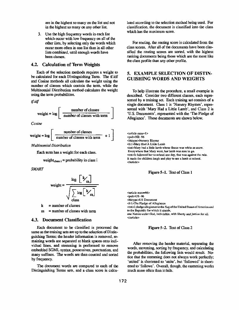
5. EXAMPLE SELECTION OF DISTIN­GUISHING WORDS AND WEIGHTS

To help illustrate the procedure, a small example is described. Consider two different classes, each repre­sented by a training set. Each training set consists of a single document Class 1 is 'Nursery Rhymes', repre­sented with 'Mary Had a Little Lamb', and Class 2 is 'U.S. Documents', represented with the 'The Pledge of Allegiance'. These documents are shown below.

<article nurn=l> <pub>NR-96 <bktype>Nursety Rhyme <hl>Mary Had A Little Lamb <txt> Mary had a little Iamb whose fleece was white as snow. Everywhere that Mary went, her lamb was sure to go. <txt> It followed her to school one day, that was against the rule. It made the children laugh and play to see a lamb at school. </article>

Figure 5-1. Text of Oass 1

<article nurn=46> <pub>US-96 <bktype>US Document <hl>The Pledge of Allegiance <txt> I pledge allegiance to the flag of the United States of America and to the Republic for which it stands, one Nation under God, indivisible, with liberty and justice for all. </article>

Figure 5-2. Text of Oass 2

Mter removing the header material, separating the words, stemming, sorting by frequency, and calculating the probabilities, the following lists would result No­tice that the stemming does not always work perlectly; 'united' is shortened to 'unite', but 'followed' is short­ened to 'followe'. Overall, though, the stemming works much more often than it fails.

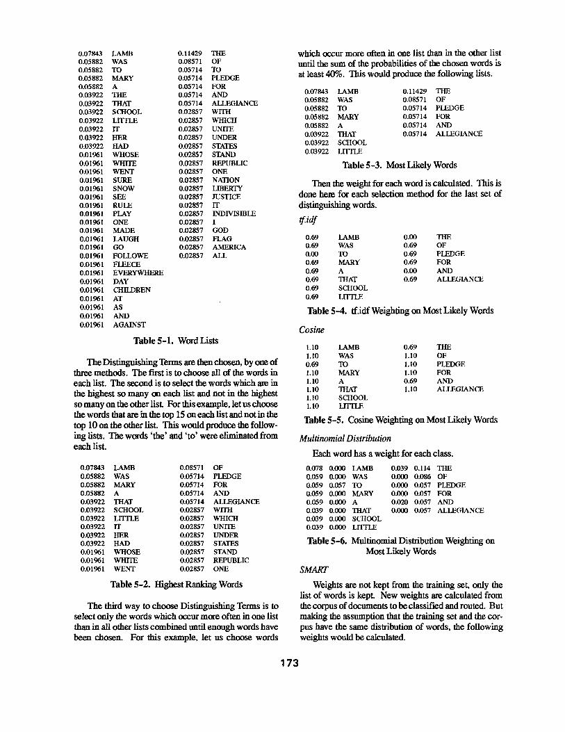
0.07843 LAMB 0.11429 TilE 0.05882 WAS 0.08571 OF 0.05882 TO 0.05714 ro 0.05882 MARY 0.05714 PLEDGE 0.05882 A 0.05714 FOR 0.03922 TilE 0.05714 AND 0.03922 THAT 0.05714 ALLEGIANCE 0.03922 SCHOOL 0.02857 WITH 0.03922 UTILE 0.02857 WHICH 0.03922 IT 0.02857 UNITE 0.03922 HER 0.02857 UNDER 0.03922 HAD 0.02857 STATES 0.01961 WHOSE 0.02857 STAND 0.01961 WHITE 0.02857 REPUBLIC 0.01961 WENT 0.02857 ONE 0.01961 SURE 0.02857 NATION 0.01961 SNOW 0.02857 LIBERIY 0.01961 SEE 0.02857 JUSTICE 0.01961 RULE 0.02857 IT 0.01961 PLAY 0.02857 INDIVISWLE 0.01961 ONE 0.02857 I 0.01961 MADE 0.02857 GOD 0.01961 LAUGH 0.02857 FLAG 0.01961 GO 0.02857 AMERICA 0.01961 FOLLOWE 0.02857 ALL 0.01961 FLEECE 0.01961 EVERYWHERE 0.01961 DAY 0.01961 CHILDREN 0.01961 AT 0.01961 AS 0.01961 AND 0.01961 AGAINST

Table 5-1. Word Lists

The Distinguishing Terms are then chosen, by one of three methods. The first is to choose all of the words in each list. The second is to select the words which are in the highest so many on each list and not in the highest so many on the other list. For this example,let us choose the words that are in the top 15 on each list and not in the top 10 on the other list. 1bis would produce the follow­ing lists. The words 'the' and 'to' were eliminated from each list.

0.07843 LAMB 0.08571 OF 0.05882 WAS 0.05714 PLEDGE 0.05882 MARY 0.05714 FOR 0.05882 A 0.05714 AND 0.03922 THAT 0.05714 ALLEGIANCE 0.03922 SCHOOL 0.02857 WITH 0.03922 UTILE 0.02857 WHICH 0.03922 IT 0.02857 UNITE 0.03922 HER 0.02857 UNDER 0.03922 HAD 0.02857 STATES 0.01961 WHOSE 0.02857 STAND 0.01961 WHITE 0.02857 REPUBLIC 0.01961 WENT 0.02857 ONE

Table 5-2. Highest Ranking Words

The third way to choose Distinguishing Terms is to select only the words which occur more often in one list than in all other lists combined until enough words have been chosen. For this example, let us choose words

which occur more often in one list than in the other list until the sum of the probabilities of the chosen words is at least 40%. This would produce the following lists.

173

0.07843 0.05882 0.05882 0.05882 0.05882 0.03922 0.03922 0.03922

LAMB WAS ro MARY A THAT SCHOOL LITILE

0.11429 0.08571 0.05714 0.05714 0.05714 0.05714

TilE OF PLEDGE FOR AND ALLEGIANCE

Table S-3. Most Likely Words

Then the weight for each word is calculated. This is done here for each selection method for the last set of distinguishing words.

tfidf

0.69 LAMB 0.00 TilE 0.69 WAS 0.69 OF 0.00 ro 0.69 PLEDGE 0.69 MARY 0.69 FOR 0.69 A 0.00 AND 0.69 THAT 0.69 ALLEGIANCE 0.69 SCHOOL 0.69 LITILE

Table S-4. tf.idf Weighting on Most Likely Words

Cosine

1.10 LAMB 0.69 TilE 1.10 WAS 1.10 OF 0.69 ro 1.10 PLEDGE 1.10 MARY 1.10 FOR 1.10 A 0.69 AND 1.10 THAT 1.10 ALLEGIANCE 1.10 SCHOOL 1.10 UTILE

Table 5-S. Cosine Weighting on Most Likely Words

Multinomial Distribution

Each word has a weight for each class.

0.078 0.000 LAMB 0.039 0.114 TilE 0.059 0.000 WAS 0.000 0.086 OF 0.059 0.057 TO 0.000 0.057 PLEDGE 0.059 0.000 MARY 0.000 0.057 FOR 0.059 0.000 A 0.020 0.057 AND 0.039 0.000 THAT 0.000 0.057 ALLEGIANCE 0.039 0.000 SCHOOL 0.039 0.000 UTILE

Table 5-6. Multinomial Distribution Weighting on Most Likely Words

SMART

Weights are not kept from the training set, only the list of words is kept. New weights are calculated from the corpus of documents to be classified and routed. But making the assumption that the training set and the cor­pus have the same distribution of words, the following weights would be calculated.

0.31 LAMB 0.00 1HE 0.31 WAS 0.42 OF 0.00 TO 0.42 PLEDGE 0.31 MARY 0.42 FOR 0.31 A 0.00 AND 0.31 TIIAT 0.42 ALLEGIANCE 0.31 SCHOOL 0.31 LITTI..E

Table S-7. SMART Weighting on Most Likely Words

6. TESTING

The methods were tested against a small set of avail­able documents. These were FBIS documents from June and July of 1991 on four different topics.

Number Topic Number of Documents

1 Vietnam: Tap Chi Cong San 20 2 Science and Technology I Japan 25 3 Arms Control 57 4 Soviet Union I Military Affairs 36

Table 6-1. Document Oasses

6.1. Selection of Distinguishing Terms

Ten documents randomly chosen from each class were used as training. These training documents were then eliminated from the set of documents to be classi­fled. The following table shows some information about the training documents.

Set Number of Words Shortest Longest Total

1 53 4445 16810 2 181 479 3118 3 161 1059 5498 4 145 6446 18191

Table 6.1-1. Document Oasses

Set 1 contained editorials from V.tetnam. Some ex­tremely short documents were included which were no longer than the header information (which was stripped before use), the title, author and source, and a note that the article was in Vietnamese and had not been trans­lated. Many of the high frequency words were political or economic.

Set 2 contained abstracts from Japanese technical papers. Many of the high frequency words were techno­logical or were Japanese locations and companies.

Set 3 contained articles about arms control from all over the world. Many of the high frequency words were location. military, or negotiation related.

Set 4 contained articles from the Soviet Union about various military affairs, including those in other coun­tries. Many of the high frequency words were Soviet Union locations or military related.

Mter experimenting with the Distinguishing Term selection methods, it was found that using the most fre­quent 300 words which were not the most frequent 300 words in any other class worked best for the tf.idf meth­od. The Cosine method worked best when the Distin­guishing Terms for each class were the words which were more likely to be in the class than in the sum of the rest of the classes, until the sum of the probabilities of the chosen words was at least 20%. The Multinomial Distribution method works best if the Distinguishing Terms for each class are more likely to be in the class than in another class, so the method which worked best was to choose the words which occur more often in one list than in all other lists combined until the sum of the probabilities of the chosen words was at least 25%.

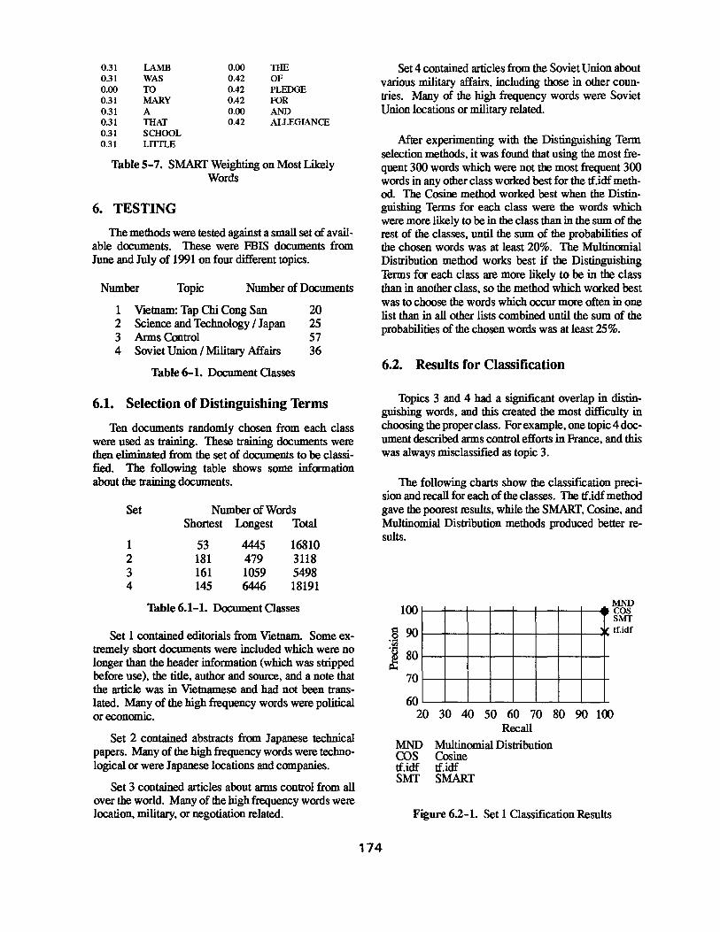
6.2. Results for Classification

Topics 3 and 4 had a significant overlap in distin­guishing words, and this created the most difficulty in choosing the proper class. For example, one topic 4 doc­ument described arms control efforts in France, and this was always misclassifted as topic 3.

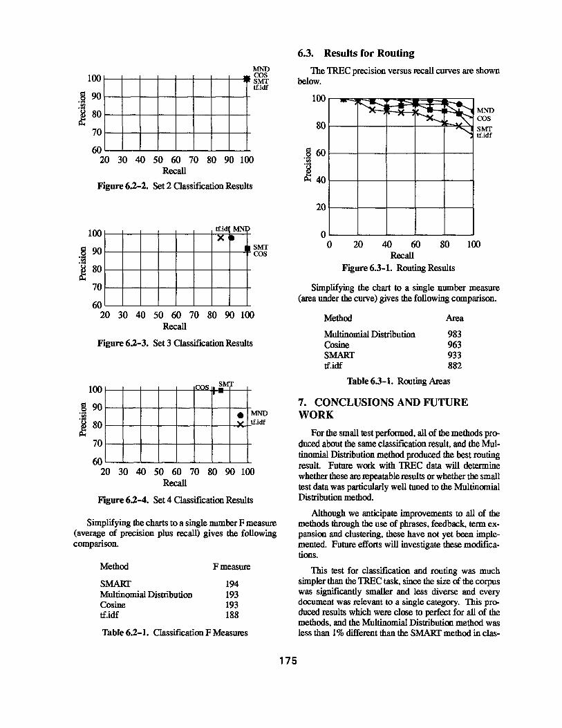
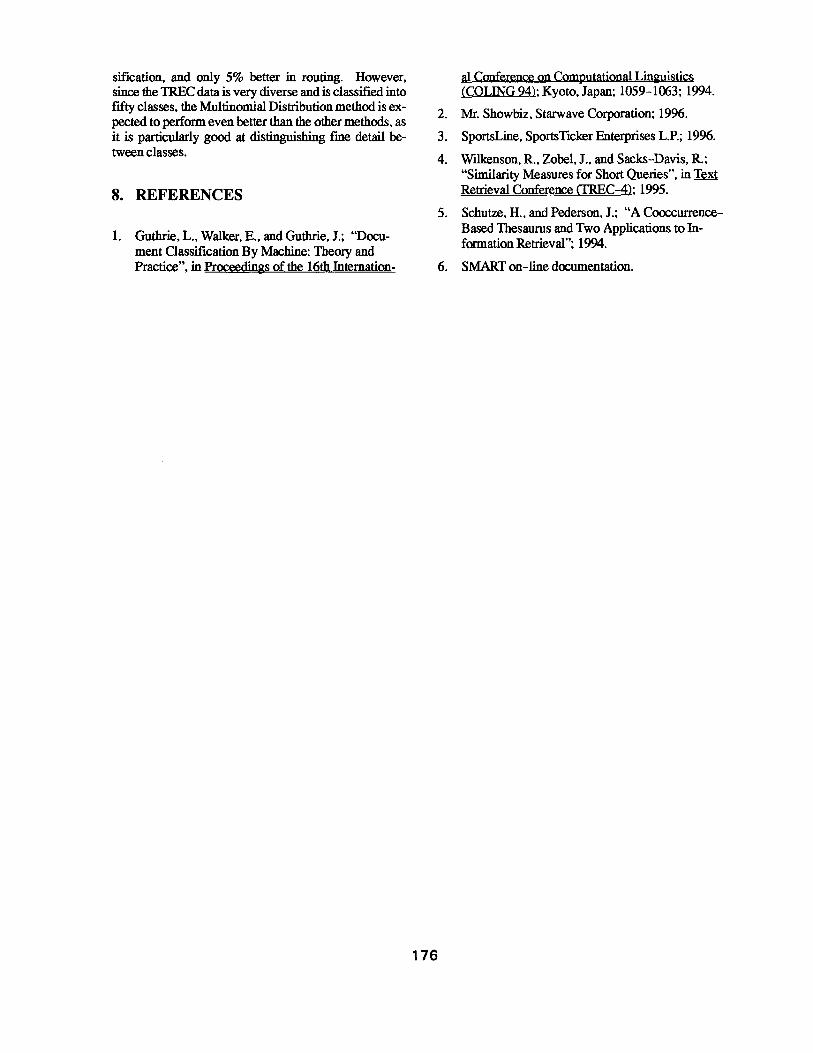
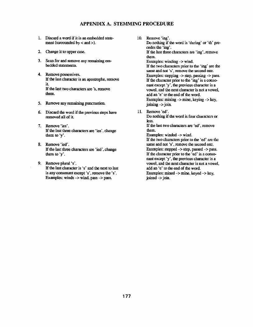
The following charts show the classification preci­sion and recall for each of the classes. The tf.idf method gave the poorest results, while the SMART, Cosine, and Multinomial Distribution methods produced better re­sults.

174

100

8 90 .....

~ 80

70

60

•if

MND cos SMT tf.idf

20 30 40 50 60 70 80 90 100 Recall

MND Multinomial Distribution COS Cosine tf.idf tf.idf SMT SMART

Figure 6.2-1. Set 1 Classification Results

MND 100 1---+-+---+--t--+--1----1--- ~m

tf.idf

8 901---+-+---+--t--t---1----1--r ..... ~ 8o~~~r-+-+-+-+-+ 70~1--+--r-~-+--r-~-+

60~~~--~~~--~~~

20 30 40 50 60 70 80 90 100 Recall

Figure 6.2-2. Set 2 Classification Results

100

8 90

j8o

70

60

tf.id

X MN:

~ I SMf

cos

20 30 40 50 60 70 80 90 100 Recall

Figure 6.2-3. Set 3 Classification Results

100

8 90 :ra ~ 80

70

60

SMf 1COS ;;.; --• v

MND tf.idf

20 30 40 50 60 70 80 90 100 Recall

Figure 6.2-4. Set 4 Classification Results

Simplifying the charts to a single number F measure (average of precision plus recall) gives the following comparison.

Method

SMART Multinomial Distribution Cosine tf.idf

Fmeasure

194 193 193 188

Table 6.2-1. Oassification F Measures

175

6.3. Results for Routing

The TREC precision versus recall curves are shown below.

100 - I ~

80

8 60 ..... rn -~

It 40

20

~ ....... ~

~ ~-......

~~ "'-J

MND cos SMf tf.idf

0 0 20 40 60 80 100

Recall Figure 6.3-1. Routing Results

Simplifying the chart to a single number measure (area under the curve) gives the following comparison.

Method

Multinomial Distribution Cosine SMART tf.idf

Area

983 963 933 882

Table 6.3-1. Routing Areas

7. CONCLUSIONS AND FUTURE WORK

For the small test performed, all of the methods pro­duced about the same classification result. and the Mul­tinomial Distribution method produced the best routing result. Future work with TREC data will determine whether these are repeatable results or whether the small test data was particularly well tuned to the Multinomial Distribution method.

Although we anticipate improvements to all of the methods through the use of phrases, feedback, term ex­pansion and clustering, these have not yet been imple­mented. Future efforts will investigate these modifica­tions.

This test for classification and routing was much simpler than the TREC task, since the size of the corpus was significantly smaller and less diverse and every document was relevant to a single category. This pro­duced results which were close to perfect for all of the methods, and the Multinomial Distribution method was less than 1% different than the SMART method in clas-

sification, and only 5% better in routing. However, since the TREC data is very diverse and is classified into f:tfty classes, the Multinomial Distribution method is ex­pected to perform even better than the other methods, as it is particularly good at distinguishing fme detail be­tween classes.

8. REFERENCES

1. Guthrie, L., Walker, E., and Guthrie, J.; "Docu­ment Oassification By Machine: Theory and Practice", in Proceedings of the 16th lntemation-

al Conference on Computational Linitlistics <COLING 94); Kyoto, Japan; 1059-1063; 1994.

2. Mr. Showbiz, Starwave Corporation; 1996.

3. SportsLine, Sports Ticker Enterprises L.P.; 1996.

4. Wilkenson, R., Zobel, J .• and Sacks-Davis, R.; "Similarity Measures for Short Queries", in Text Retrieval Conference ITREC-4); 1995.

176

5. Schutze, H., and Pederson, J.; "A Cooccurrence­Based Thesaurus and Two Applications to In­formation Retrieval"; 1994.

6. SMART on-line documentation.

APPENDIX A. STEMMING PROCEDURE

1. Discard a word if it is an embedded state- 10. Remove 'ing'. ment (surrounded by < and>). Do nothing if the word is 'during' or 'th' pre-

cedes the 'ing'. 2. Change it to upper case. If the last three characters are 'ing'. remove

them. 3. Scan for and remove any remaining em- Examples: winding-> wind.

bedded statements. If the two characters prior to the 'ing' are the same and not 's', remove the second one.

4. Remove possessives. Examples: stepping-> step, passing-> pass. If the last character is an apostrophe, remove If the character prior to the 'ing' is a conso-it. nant except 'y'. the previous character is a If the last two characters are 's, remove vowel. and the next character is not a vowel, them. add an 'e' to the end of the word.

5. Remove any remaining punctuation. Examples: mining ->mine, keying ->key, joining-> join.

6. Discard the word if the previous steps have 11. Remove 'ed'. removed all of it. Do nothing if the word is four characters or

less. 7. Remove 'ies'. If the last two characters are 'ed'. remove

If the last three characters are 'ies', change them. them to 'y'. Examples: winded -> wind.

If the two characters prior to the 'ed' are the 8. Remove 'ied'. same and not's'. remove the second one.

If the last three characters are 'ied'. change Examples: stepped-> step, passed ->pass. them to 'y'. If the character prior to the 'ed' is a conso-

nant except 'y'. the previous character is a 9. Remove plural 's'. vowel, and the next character is not a vowel,

If the last character is 's' and the next to last add an 'e' to the end of the word. is any consonant except's', remove the's'. Examples: mined-> mine. keyed-> key, Examples: winds -> wind. pass ->pass. joined-> join.

177