Embed Size (px)
Citation preview

Clayton School of Information Technology
Monash University
Clayton VIC 3800, Australia
Technical Report No. 2010/256
A Simple Gradient-based Metric LearningAlgorithm for Object Recognition
Nayyar A. Zaidi, David McG. Squire, and David Suter

Abstract
The Nearest Neighbor (NN) classification/regression techniques, besides their sim-plicity, is one of the most widely applied and well studied techniques for patternrecognition in machine learning. Their only drawback is the assumption of the avail-ability of a proper metric used to measure distances to k nearest neighbors. It hasbeen shown that K-NN classifier’s with a right distance metric can perform better thanother sophisticated alternatives like Support Vector Machines (SVM) and GaussianProcesses (GP) classifiers. That’s why recent research in k-NN methods has focusedon metric learning i.e., finding an optimized metric. In this paper we have proposed asimple gradient based algorithm for metric learning. We discuss in detail the motiva-tions behind metric learning, i.e., error minimization and margin maximization. Ourformulation is different from the prevalent techniques in metric learning where goal isto maximize the classifier’s margin. Instead our proposed technique (MEGM) findsan optimal metric by directly minimizing the mean square error. Our technique notonly resulted in greatly improving k-NN performance but also performed better thancompeting metric learning techniques. We also compared our algorithm’s performancewith that of SVM. Promising results are reported on major faces, digits, object andUCIML databases.
1 Introduction
Nearest neighbor methods for pattern recognition have been proven to be very usefulin machine learning. Despite the simplicity, their performance is comparable to othersophisticated classification and regression techniques like Support Vector Machines (SVM)and Guassian Process (GP) and they have been widely applied for a huge variety ofproblems. Computer vision research has benefited greatly from advancements in nearestneighbor methods, for example some state-of-the-art techniques for object recognition arebased on nearest neighbor analysis (1),(2). For a given query point, a nearest neighborclassifier works by assigning it the label of the majority class in its neighborhood.
It is self evident that k-NN classifier’s simplicity leads to one of its major pros. A k-NN classifier deals with multi-class classification scenario effortlessly. On the other handwe need one-versus-one and one-versus-all techniques to deal with multi-class scenarioin case of binary classifiers like SVM. This makes them computationally expensive. Ask-NN classification involves no training they are computational efficient. But still theeffectiveness of k-NN methods stems from their asymptotic properties. The asymptoticresults in (3), (4), (5) suggests that a 1-NN method based on a simple Euclidean distancewill perform well provided the number of training samples is not too small. And 1-NNwill achieve the performance of a Bayes Optimal classifier as the number of training databecomes very large. These asymptotic results are based on the fact that bias in theprediction of function f(x) becomes vanishingly small if the number of training data Nis large with few features p i.e., N >>> p. But typical machine learning data has largenumber of features and data required to validate these asymptotic results is humongouswhich is not feasible. This is also known as Curse-of-Dimensionality (COD). Also due toCOD most of the data points are very far apart and k-NN neighborhoods are no longer‘local’, refer to section 2.5 in (6). Therefore we need to modify distances in high dimensionsto alleviate the COD, reduce bias and make neighborhood local. This calls for tuning ametric and hence metric learning.
As discussed, the performance of a nearest neighbor classifier depends critically on twomajor factors: (a) the distance metric used and (b) size of the neighborhood (specified byK which denotes the number of nearest neighbors). The value of K controls the MeanSquare Error (MSE) which is defined as MSE = bias2 + var. Small K implies small biasbut high variance and vice-versa. Since K is specified in terms of the number of nearestneighbors of a query point x which implicitly depends on a distance measure, MSE can
1

Figure 1: Contrived example demonstrating the impact of metric on margin
be controlled by estimating a distance metric (a metric is generally specified through anorm and a positive semi-definite matrix). Typically we estimate the inverse square rootsof metric. That is we learn a matrix parameterizing the linear transformation of theinput space such that in the transformed space k-NN performs well. If we denote suchtransformation by a matrix A, we are effectively learning a metric defined by ATA suchthat d(x, y) = (x− y)ATA(x− y) = (Ax−Ay)T (Ax−Ay).
In the current research on nearest neighbor methods, a dichotomy exists for metriclearning methods in terms of their goals. Most ‘Metric Learning’ algorithms aim at findinga metric that results in small intra-class and large inter-class distances (7), (8), (9), (10),(11), (12). This results in maximizing the margin 1. Figure 1 depicts a simple contrivedexample of data belonging to two classes represented by red and blue dots. As can beseen that the classes are linearly separable and a hyper-plane is represented by a darkblack line. In this scenario, margin can be maximized in two ways, either we modify thehyper-plane to better fit the training data or we transform the training data to maximizemargin with respect to a certain hyper-plane. The later has been the goal of most metriclearning algorithms. SVMs on the other hand optimizes margin by finding an optimalhyper-plane. They are designed to minimize empirical risk with a bound on generalizationerror. Metric learning can also be used to minimize empirical risk i.e., maximizing themargin by modifying hyper-plane. Such a kind of strategy has been introduced in (13)where metric learning has been employed as bias reduction strategy and reducing MSE tobetter fit training data.
In this paper we have presented a novel metric learning algorithm with the goals ofmaximizing the margin by reducing MSE directly. We propose a simple MSE gradient min-imization (MEGM - Mean square Error’s Gradient Minimization) approach for improvingthe performance of k-NN neighbor classifier. Our method is based on gradient descentof MSE objective function. We compared MEGM’s performance with other metric learn-ing approaches for margin maximization for example neighborhood component analysis(NCA). As will be shown in section 4 our method not only results in significant improve-ment in the performance of k-NN classifier but also outperforms other metric learningalgorithm on most data-sets. As we will discuss in section 5, unlike SVM we minimize theempirical risk only. We have not catered for generalization in our algorithm. But in ourexperiments we did not experience any over-fitting. The inclusion of generalization termcan be introduced in our framework and has been left as a future work.
Rest of the paper is organized as follows: we will discuss related work in section 2. Ourproposed MEGM algorithm is described in detail in section 3. Detail description aboutexperimental setup and comparison results on UCIML, face, object and digits data-sets
1The margin of a point is defined as the distance between the point and the closest point on theclassification boundary
2
are given in section 4. We conclude in section 5 with pointers on future work.
2 Related Work
Our proposed algorithm MEGM is very close in nature to (14) where a gradient basedtechnique is used for selecting relevant features. That is, only diagonal terms of thecovariance matrix are estimated. In our method we learn a full covariance matrix ratherthan estimating only diagonal terms. Thats why MEGM is superior to technique proposedin (14).
The other notable techniques for metric learning are LMNN (15), RCA (16) and NCA(7). Relevant Component Analysis (RCA) (16) constructs a Mahalanobis distance metricfrom a weighted sum of in-class covariance matrices. It is similar to Principal ComponentAnalysis (PCA) and Linear Discriminant Analysis (LDA) in its reliance on second orderstatistics. Large Margin Nearest Neighbor (LMNN) algorithm in (15) is posed as a convexproblem, and thus the reach of the global solution is guaranteed. However, a specialoptimization solver is needed for efficient implementation.
Neighborhood Component Analysis (NCA) (7) maximizes margin by minimizing theprobability of error under stochastic neighborhood assignment. In particular each pointi selects another point j as its neighbor with some probability pij , and inherits its classlabels from the point it selects. pij is defined as a softmax over Euclidean distances in thetransformed space, parameterized by A:
pij =− exp(‖Axi −Axj‖2)∑k 6=i exp(−‖Axi −Axk‖2)
(1)
NCA maximizes the pij in above equation by finding an optimal A matrix. That isthe probability of the number of points correctly classified is maximized.
The comparison of our proposed algorithm (MEGM) with NCA has been a majormotivation of this work. Though NCA is sound in theory, our empirical results in section 4suggests that MEGM performs better than NCA on most data-sets. We will mention insection 5 about an approach to combine both MEGM and NCA to improve MEGM’sgeneralization capacity.
3 Approach
In a typical regression setting, an unknown function f : RD → R is predicted from thetraining data {(~x1, y1), (~x2, y2), ...(~xN , yN )}, where ~xi is a data point and y is the corre-sponding target value. The predicted function f is chosen to be the one that minimizessome loss function such as ‘mean squared error’ (MSE) etc. The MSE for a data setcontaining N of points is given in the following equation:
MSE(f) =N∑
i=1
(f(~xi)− f(~xi))2 (2)
For classification task having T classes we can replace above error function as:
MSE(y) =T∑
t=1
N∑i=1
(yti − yti) (3)
where yi denotes the predicted probability of point ~xi and yi denotes the true label (either0 or 1) of point ~xi. For brevity we have denoted y( ~xti) with yti and y( ~xti) with yti. In the
3

following discussion we will assume that there are only two classes to make our derivationssimple. For any query point ~xi, nearest neighbor methods work by predicting the value yi
by considering the labels of its k nearest neighbors. In order to have a smooth boundary,each neighbor votes for the query label based on its distance from the query point (referto (6) for details). Equation 4 shows the Nadaraya-Watson kernel for regression:
y(~x) =∑
j yjVj∑j Vj
(4)
The vote Vj casted by each label around the query point ~x is usually chosen to be a functionthat decays exponentially as the distance from the query point increases, for example aGaussian kernel:
Vj = exp(−d(~x, ~xj)
2σ2
)(5)
Determining votes using equation 5 assumes a well defined distance measure. This assump-tion, as discussed in the previous section, is not always true, due to the COD and irrelevantfeatures, and can lead to bad results. d(~x, ~xj) in equation 5 can be replaced by a moregeneral metric: that is dL(~x, ~xj). If L = ATA, then dL(~x, ~xj) = (A~x−A~xj)T (A~x−A~xj).Since MSE is a function of y and y depends on ||~x − ~xj ||2L, MSE can be minimized byselecting an optimal value of L. In other words, a change in the L induces a change in thedistance, which can alter the votes. This alteration in the votes Vj triggers a change in yaffecting the MSE. It is more helpful to optimize A rather than L, because optimizationfor L requires to fulfill semi-positive constraint which is expensive to maintain. Obviouslytrying all possible values of A is not feasible. Some sort of search mechanism is requiredto find an optimal value of A. Votes Vj in equation 5 can be replaced by Wj as:
Wj = exp
(−‖A~x−A~xj‖22
2σ2
)(6)
The proposed gradient based technique (MEGM) is based on a gradient descent al-gorithm to minimize MSE (lets denote by EA). The gradient EA is evaluated to find anoptimal A matrix. Convergence to the global minimum is not guaranteed. The risk oflocal minima can be reduced by running the algorithm several times and choosing theoutput with minimum error EA. The gradient of EA with respect to matrix A is:
∂E
∂A= (yi − yi)
1∑j Wj
∑j
(yj − yj))∂Wj
∂A(7)
The size of the gaussian kernel centered at the query point (σ in equation 6) is set propor-tional to the distance of the k nearest neighbors. Generally the average distance of halfof the nearest neighbors is used, as this measure is more stable under a varying distancemetric:
σ2 =12
1P
P∑p=1
‖~x− ~xp‖2 where P = k/2 (8)
∂Wj
∂A in equation 7 can be derived as:
∂Wj
∂A= 2WjA(~x− ~xj)(~x− ~xj)T (9)
Combining equations 7 and 9 we can write the gradient of EA with respect to matrix Aas:
∂E
∂A= 2A(yi − yi)
1∑j Wj
∑j
(yj − yj)Wj(~x− ~xj)(~x− ~xj)T (10)
4

Equation 10 represents the gradient of the error function with respect to matrix A whichis minimized to get an optimal A. The Polack-Ribiere flavour of conjugate gradients isused to compute search directions, and a line search using quadratic and cubic polynomialapproximations and the Wolfe-Powell stopping criteria is used together with the sloperatio method for guessing initial step sizes.
4 Experimental Results
In this section we present results on various machine learning databases from UCIMLrepository (17), face, object and digit databases. Database details such as number ofdata, features and classes as well as experimental setup details such as number of data percategory used for training and testing and the number of eigen vectors used are given intable 1. For faces (yalefacs, yalefaceB, AT&T, caltechfaces, caltechfacesB), digit (USPS),Object (Coil100) and Isolet data-set, not only we have compared MEGM’s performancewith standard k-NN classifier but also with SVM. MEGM’s results are also compared withother metric learning approaches like NCA, RCA and LMNN.
To obtain SVM results, multi-class SVM with gaussian kernel is used. C parameterfor SVM are tuned through cross-validataion. σ parameter is set to the average distanceof k nearest neighbor as this approach has been shown to be more efficient for objectdatabases as shown in (18). For obtaining multi-class SVM results, one-versus-all strategyis employed. Each experiment (except for UCIML databases) is repeated 10 times andmean results and standard deviations are presented.
Faces, USPS, Coil100 and Isolet data-sets are also pre-processed for efficiency. Pre-processing images using PCA is a common approach in object recognition research toreduce dimensionality. This results in vastly reduced computational cost. In our experi-ments, the results are obtained by reducing the dimensionality of data set by projectingdata on first few eigenfaces. Number of eigenfaces used for each database is given intable 1. We have not investigated results without pre-processing images, that is usinggray-scale values as features due to computational cost. No pre-processing is done forUCIML databases. The size of neighborhood (k) as discussed in section 3 is consistentlyset equal to the log2(cardinality of data set) for all databases.
Database #Data #Features #Classes PCA #Train/Class #Test/Classyalefaces 165 77760 15 50 4 7
yalefacesB 5850 307200 10 20 10 20caltechfaces 435 47500 29 30 5 10
caltechfacesB 435 47500 2 30 50 100AT&Tfaces 400 10304 40 50 5 5
Coil100 7200 16384 100 50 10 10USPS 9298 256 10 50 20 10Isolet 6238 617 26 30 20 10
Table 1: Details of Face, Object and Digit Databases used for classification
To obtain the final classification results, one nearest neighbor (1-NN) classification isused. As mentioned in section 3, since both NCA and MEGM suffers from local minimaproblems, some care has to be taken to make sure that it does not effect results. ForUCIML and other databases, we run MEGM and NCA thrice with different training datasamples and selected the best results. In order to make sure that our results are not biasedto NCA and MEGM due to this procedure, reported results for all other techniques forexample k-NN, SVM, LMNN and RCA are computed this way. That is each method is run
5
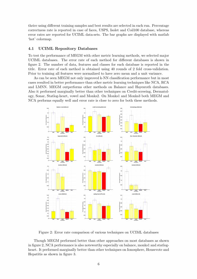
thrice using different training samples and best results are selected in each run. Percentagecorrectness rate is reported in case of faces, USPS, Isolet and Coil100 database, whereaserror rates are reported for UCIML data-sets. The bar graphs are displayed with matlab‘hot’ colormap.
4.1 UCIML Repository Databases
To test the performance of MEGM with other metric learning methods, we selected majorUCIML databases. The error rate of each method for different databases is shown infigure 2. The number of data, features and classes for each database is reported in thetitle. Error rate of each method is obtained using 40 rounds of 2 fold cross-validation.Prior to training all features were normalized to have zero mean and a unit variance.
As can be seen MEGM not only improved k-NN classification performance but in mostcases resulted in better performance than other metric learning techniques like NCA, RCAand LMNN. MEGM outperforms other methods on Balance and Hayesroth databases.Also it performed marginally better than other techniques on Credit-screeing, Dermatol-ogy, Sonar, Statlog-heart, vowel and Monks2. On Monks1 and Monks3 both MEGM andNCA performs equally well and error rate is close to zero for both these methods.
KNN RCA LMNN MEGM NCA0
0.05
0.1
0.15
0.2
0.25
Techniques
Pe
rce
nta
ge
Pe
rfo
rma
nce
balance−scale (625,4,3)
KNN RCA LMNN MEGM NCA0
0.05
0.1
0.15
0.2
0.25
Techniques
Perc
en
tag
e P
erf
orm
an
ce
credit screening (653,15,2)
KNN RCA LMNN MEGM NCA0
0.01
0.02
0.03
0.04
0.05
0.06
0.07
0.08
Techniques
Perc
en
tag
e P
erf
orm
an
ce
dermatology (358,34,6)
KNN RCA LMNN MEGM NCA0
0.05
0.1
0.15
0.2
0.25
0.3
0.35
0.4
0.45
0.5
Techniques
Perc
en
tag
e P
erf
orm
an
ce
hayesroth (135,5,3)
KNN RCA LMNN MEGM NCA0
0.01
0.02
0.03
0.04
0.05
0.06
Techniques
Perc
en
tag
e P
erf
orm
an
ce
iris (150,4,3)
KNN RCA LMNN MEGM NCA0
0.02
0.04
0.06
0.08
0.1
0.12
Techniques
Pe
rce
nta
ge
Pe
rfo
rma
nce
liver−disorder (345,6,2)
KNN RCA LMNN MEGM NCA0
0.05
0.1
0.15
0.2
0.25
0.3
Techniques
Perc
en
tag
e P
erf
orm
an
ce
monks1 (432,6,2)
KNN RCA LMNN MEGM NCA0
0.05
0.1
0.15
0.2
0.25
0.3
Techniques
Perc
en
tag
e P
erf
orm
an
ce
monks2 (432,6,2)
KNN RCA LMNN MEGM NCA0
0.05
0.1
0.15
0.2
0.25
Techniques
Perc
en
tag
e P
erf
orm
an
ce
monks3 (432,6,2)
KNN RCA LMNN MEGM NCA0
0.05
0.1
0.15
0.2
0.25
0.3
0.35
0.4
0.45
Techniques
Perc
en
tag
e P
erf
orm
an
ce
sonar (208,60,2)
KNN RCA LMNN MEGM NCA0
0.05
0.1
0.15
0.2
0.25
0.3
0.35
Techniques
Perc
en
tag
e P
erf
orm
an
ce
statlog heart (270,13,2)
KNN RCA LMNN MEGM NCA0
0.02
0.04
0.06
0.08
0.1
0.12
Techniques
Perc
en
tag
e P
erf
orm
an
ce
vowel (528,2,10)
Figure 2: Error rate comparison of various techniques on UCIML databases
Though MEGM performed better than other approaches on most databases as shownin figure 2, NCA performance is also noteworthy especially on balance, monks1 and statlog-heart. It performed marginally better than other techniques on Ionosphere, Housevote andHepatitis as shown in figure 3.
6

KNN RCA LMNN MEGM NCA0
0.05
0.1
0.15
0.2
0.25
Techniques
Perc
en
tag
e P
erf
orm
an
ce
hepatitis (80,19,2)
KNN RCA LMNN MEGM NCA0
0.01
0.02
0.03
0.04
0.05
0.06
0.07
0.08
0.09
0.1
Techniques
Perc
en
tag
e P
erf
orm
an
ce
house vote (232,16,2)
KNN RCA LMNN MEGM NCA0
0.02
0.04
0.06
0.08
0.1
0.12
0.14
0.16
0.18
0.2
Techniques
Perc
en
tag
e P
erf
orm
an
ce
ionosphere (352,34,2)
Figure 3: Error rate comparison of various techniques on UCIML databases, NCA performsbest on these data-sets
4.2 Face Databases
We have experimented with 5 face databases. Yalefaces, YalefacesB, AT&T and cal-techfaces were used to compare the performance of MEGM with margin based metriclearning algorithm (NCA) and other classification techniques like k-NN and SVM. Detailsof these databases are given in table 1. Yalefaces, YalefacesB, AT&T are well-known inface recognition research. The Yalefaces database (19) contains 165 grayscale images of15 individuals. There are 11 images per subject, one per different facial expression orconfiguration: center-light, with glasses, happy, left-light, with no glasses, normal, right-light, sad, sleepy, surprised, and wink. The YalefacesB database (20) contains 5760 singlelight source images of 10 subjects each seen under 576 viewing conditions (9 poses x 64illumination conditions). For every subject in a particular pose, an image with ambient(background) illumination was also captured. AT&T database (21) has ten different im-ages of each of 40 distinct subjects. For some subjects, the images were taken at differenttimes, varying the lighting, facial expressions (open, closed eyes, smiling, not smiling) andfacial details (glasses, no glasses). All the images were taken against a dark homogeneousbackground with the subjects in an upright, frontal position (with tolerance for some sidemovement)
Caltechfaces and CaltechfacesB constitutes images from face category in Caltech-101object database (22). Caltech-101 face category has 435 images of around 20 people.Some example images are shown in figure 4. Caltechfaces database in table 1 is based onsplitting Caltech-101 face category in 20 categories, each belonging to different person. Onthe other hand, CaltechfacesB in table 1 is based on splitting Caltech-101 face categoryin two classes only, male and female.
Figure 4: Example images from caltechfaces and caltechfacesB
The SVM results are obtained by optimizing over C parameter. C is searched from thevalues: 1, 10, 100, 1000. The comparative results on face databases are shown in figure 5where percentage performance is reported. As can be seen that MEGM results in signifi-cant improvements in k-NN classification and outperforms NCA on all databases. Thoughperformance gain of MEGM over SVM is not substantial, given that SVM is trained withC parameter optimized through cross-validation, our results are encouraging.
7

KNN MEGM−KNN SVM NCA60
65
70
75
80
85
90
95
TechniquesPe
rcen
tage
Per
form
ance
yalefaces
(a)
KNN MEGM−KNN SVM NCA90
91
92
93
94
95
96
97
98
99
100
Techniques
Perc
enta
ge P
erfo
rman
ce
yalefacesB
(b)
KNN MEGM−KNN SVM NCA90
91
92
93
94
95
96
97
98
99
100
Techniques
Perc
enta
ge P
erfo
rman
ce
AT&Tfaces
(c)
KNN MEGM−KNN SVM NCA70
75
80
85
90
95
100
Techniques
Perc
enta
ge P
erfo
rman
ce
caltechfaces
(d)
KNN MEGM−KNN SVM NCA80
82
84
86
88
90
92
94
96
98
100
Techniques
Perc
enta
ge P
erfo
rman
ce
caltechfacesB
(e)
Figure 5: Percentage performance of different techniques on different face databases
4.3 USPS Database
The USPS digits data was gathered at the Center of Excellence in Document Analysis andRecognition (CEDAR) at SUNY Buffalo, as part of a project sponsored by the US PostalService (23). Sample images from USPS digit data-set is shown in figure 6. Results on
2 4 6 8 10 12 14 16
2
4
6
8
10
12
14
16
2 4 6 8 10 12 14 16
2
4
6
8
10
12
14
16
2 4 6 8 10 12 14 16
2
4
6
8
10
12
14
16
2 4 6 8 10 12 14 16
2
4
6
8
10
12
14
16
2 4 6 8 10 12 14 16
2
4
6
8
10
12
14
16
2 4 6 8 10 12 14 16
2
4
6
8
10
12
14
16
2 4 6 8 10 12 14 16
2
4
6
8
10
12
14
16
2 4 6 8 10 12 14 16
2
4
6
8
10
12
14
16
2 4 6 8 10 12 14 16
2
4
6
8
10
12
14
16
2 4 6 8 10 12 14 16
2
4
6
8
10
12
14
16
2 4 6 8 10 12 14 16
2
4
6
8
10
12
14
16
2 4 6 8 10 12 14 16
2
4
6
8
10
12
14
16
2 4 6 8 10 12 14 16
2
4
6
8
10
12
14
16
2 4 6 8 10 12 14 16
2
4
6
8
10
12
14
16
2 4 6 8 10 12 14 16
2
4
6
8
10
12
14
16
2 4 6 8 10 12 14 16
2
4
6
8
10
12
14
16
2 4 6 8 10 12 14 16
2
4
6
8
10
12
14
16
2 4 6 8 10 12 14 16
2
4
6
8
10
12
14
16
2 4 6 8 10 12 14 16
2
4
6
8
10
12
14
16
2 4 6 8 10 12 14 16
2
4
6
8
10
12
14
16
Figure 6: Example images from USPS database
USPS dataset are shown in figure 7(a). We did not find any noticeable increase in k-NNperformance on USPS database. Though MEGM marginally improves k-NN performance,SVM performs the best. NCA on the hand did not result in any performance gain. SVMresults are optimized over C values of {1, 10, 100, 1000}.
4.4 Isolet Database
Isolet (Isolated Letter Speech Recognition) (17) consists of 26 categories. 120 subjectsspoke the name of each letter of the alphabet twice. Hence, we have 52 training examples
8

KNN MEGM−KNN SVM NCA70
75
80
85
90
95
TechniquesPe
rcen
tage
Per
form
ance
USPS
(a)
KNN MEGM−KNN SVM NCA70
75
80
85
90
95
Techniques
Perc
enta
ge P
erfo
rman
ce
Isolet
(b)
Figure 7: Percentage performance of different techniques on USPS and Isolet databases
Figure 8: Sample images from Coil Object database.
from each speaker. Results on Isolet database is shown in figure 7(b). MEGM, SVM andNCA resulted in k-NN performance on Isolet database. Like USPS, SVM outperforms ourmethod on this database. MEGM performs better than NCA. Similar to faces and USPSdatasets, SVM results are optimized over C values of {1, 10, 100, 1000}.
4.5 Coil100 Database
Coil100 object database consists of 100 object categories (24). Each category has 72images taken at different angle of the object. Figure 7 shows results on Coil100 database.Using MEGM and NCA we got some improvement over k-NN performance. SVM did notperform well on this database with only 81% success rate as compared to k-NN method of86% success rate. NCA also deteriorated k-NN results. The SVM results were obtainedby searching for C value from {1, 10, 100, 1000}.
KNN MEGM−KNN SVM NCA70
75
80
85
90
95
Techniques
Perc
enta
ge P
erfo
rman
ce
Coil100
Figure 9: Percentage performance of different techniques on Coil100 object databases
9
5 Conclusion
The main pro of our proposed MEGM algorithm is its simplicity. As discussed, MEGMminimizes MSE gradient using a simple gradient descent algorithm. MEGM improvesk-NN classification by learning a data dependent distance metric and performs as well asSVM on most if not all databases. Also It deals with multi-class problems effortlessly asopposed to binary classifiers like SVM where a one-versus-one and one-versus-all strategyis used. As discussed, SVM’s training and testing is computationally expensive, for ex-ample it takes very long time to train and test an SVM classifier on Coil100 database. Astraining involves training 100 classifiers and for classifying an image, all classifiers votefor prediction. On the other hand, once a metric is learnt using MEGM, a simple nearestneighbor classification is required. In typical object recognition tasks where number ofclasses are very large, nearest neighbor methods should be preferable for their computa-tional efficiency. Therefore k-NN methods equipped with a proper distance metric (forexample, one trained with MEGM) can be extremely useful.
A drawback of MEGM includes local minima problem. Standard approaches to avoidlocal minima are to be used. Also one is tempted to think of over-fitting if the objectivefunction is only MSE. In this work we did not encounter any over-fitting. As a futurework we are investigating to modify our objective function to include a generalizationterm, that is penalize large changes in A matrix to avoid over-fitting. We are currentlyinvestigating to combine MEGM’s and NCA’s objective function to improve our results.As in this study, MEGM which is based on the minimization of MSE resulted in betterperformance than NCA and other metric learning algorithms which maximizes marginexplicitly, a natural extension to the proposed method is to combine the two approaches.That is learn a metric by simultaneously maximizing the margin and minimizing the MSE.The objective functions of MEGM and NCA is combined in the following equation:
EA =N∑
i=1
(yi − exp
(−‖A~x−A~xj‖22
2σ2
))+
(exp(‖Axi −Axj‖2)∑
k 6=i exp(−‖Axi −Axk‖2)
)(11)
We are investigating gradient based methods to optimize for A in equation 11. Asimple gradient based strategy as employed in MEGM can be used. Considering theMEGM results, the combination with NCA can lead to good results.
There has been a lot of work done in adaptive distance metric (25), (26), (27). Inadaptive metric learning a separate metric is learnt for each query point. We are currentlymodifying MEGM to work in such local settings. Training a separate metric for each querypoint can become computationally expensive. We are investigating clustering techniquesto cluster data first and than train a separate metric for each cluster.
In summary, we proposed a simple mean square error’s gradient based metric learningalgorithm (MEGM) in this paper and showed that MEGM not only results in classificationimprovement of k-NN classifier but also perform better than other metric learning algo-rithms. The results are also compared with state-of-the-art classifier, SVM. Results areshown on major UCIML, face, digits and object databases. Our results are encouragingand requires additional investigation to further improve MEGM performance as describedabove.
References
[1] A. Frome, Y. Singer, and J. Malik, “Image retrieval and classification using localfunctions,” in NIPS, 2006.
10
[2] M. Nilsback and A. Zisserman, “A visual vocabulary for flower classification,” inCVPR, 2006.
[3] T. Cover, “Rates of convergence for nearest neighbor procedures,” in Inter. Conf. onSystems Sciences, 1968.
[4] E. Fix and J. Hodges, “Discriminatory analysis - nonparameteric discrimination: con-sistency properties,” Tech Report, Randolph Field Texas, US Airforce School of Avi-ation Medicine, Tech. Rep., 1951.
[5] R. Snapp and S. Venkatesh, “Asymptotic expansions of the k-nearest neighbor risk,”The Annals of Statistics, 1998.
[6] T. Hastie, R. Tibshirani, and J. Friedman, The Elements of Statistical Learning.Springer Series in Statistics, 2001.
[7] J. Goldberger, S. Roweis, G. Hinton, and R. Salakhutdinov, “Neighborhood compo-nent analysis,” in NIPS, 2005.
[8] J. Davis and I. Dhillon, “Structured metric learning for high dimensional problems,”in KDD, 2008.
[9] K. Weinberger, J. Blitzer, and L. Saul, “Distance metric learning for large marginnearest neighbor classification,” in NIPS, 2005.
[10] B. Sriperumbudar, O. Lang, and G. Lanckriet, “Metric embedding for kernel classi-fication rules,” in ICML, 2008.
[11] A. Globerson and S. Roweis, “Metric learning by collapsing classes,” in NIPS, 2005.
[12] E. Xing, A. Ng, M. Jordan, and S. Russell, “Distance metric learning with applicationto clustering with side-information,” in NIPS, 2002.
[13] J. Friedman, “Flexible metric nearest neighbor classification,” Tech Report, Dept. ofStatistics, Stanford University, Tech. Rep., 1994.
[14] D. Lowe, “Similarity metric learning for a variable-kernel classifier,” in NIPS, 1996.
[15] K. Weinberger, J. Blitzer, and L. Saul, “Distance metric learning for large marginnearest neighbor classification,” in NIPS, 2006.
[16] A. Bar-Hillel, T. Hertz, N. Shental, and D. Weinshall, “Learning distance functionsusing equivalence relation,” in ICML, 2003.
[17] C. Mertz and P. Murphy, “Machine learning repository,” 2005. [Online]. Available:http://archive.ics.uci.edu/ml/
[18] J. Zhang, M. Marszalek, S. Lazebnik, and C. Schmid, “Local features and kernels forclassification of texture and object categories: A comprehensive study,” in CVPRW,2006.
[19] “The yale face database,” 1997. [Online]. Available:http://cvc.yale.edu/projects/yalefaces/yalefaces.html
[20] “The yale face b database,” 2001. [Online]. Available:http://cvc.yale.edu/projects/yalefacesB/yalefacesB.html
[21] “The at&t face database,” 2002. [Online]. Available:http://www.cl.cam.ac.uk/research/dtg/attarchive/facedatabase.html
11
[22] “Caltech-101 object database,” 2006. [Online]. Available:http://www.vision.caltech.edu/Image Datasets/Caltech101/
[23] J. Hull, “A database for handwritten text recognition research,” IEEE PAMI, 1994.
[24] S. Nene, S. Nayar, and H. Murase, “Columbia object image library (coil-100),” Tech-nical Report CUCS-006-96, February 1996, Tech. Rep., 1996.
[25] T. Hastie and R. Tibshirani, “Discriminative adaptive nearest neighbor classifica-tion,” IEEE transactions on Pattern Analysis and Machine Intelligence, 1996.
[26] C. Domenciconi, J. Peng, and D. Gunopulos, “An adaptive metric machine for patternclassification,” in NIPS, 2000.
[27] N. Zaidi, D. Squire, and D. Suter, “BoostML: An adaptive metric learning for nearestneighbor classification,” in PAKDD, 2010.
12