A simple and efficient parallel FFT algorithm

using the BSP model ⋆

Marcia A. Inda

FOM Institute for Atomic and Molecular Physics (AMOLF), Kruislaan 407, 1098SJ Amsterdam, The Netherlands

andInstituto de Matematica, Universidade Federal do Rio Grande do Sul, Av. Bento

Goncalves 9500, 91509-900 Porto Alegre, RS, Brazil

Rob H. Bisseling

Department of Mathematics, Utrecht University, PO Box 80010, 3508 TA Utrecht,The Netherlands

Abstract

We present a new parallel radix-4 FFT algorithm based on the BSP model. Ourparallel algorithm uses the group-cyclic distribution family, which makes it simpleto understand and easy to implement. We show how to reduce the communicationcost of the algorithm by a factor of three, in the case that the input/output vectoris in the cyclic distribution. We also show how to reduce computation time oncomputers with a cache-based architecture. We present performance results on aCray T3E with up to 64 processors, obtaining reasonable efficiency levels for localproblem sizes as small as 256 and very good efficiency levels for local sizes largerthan 2048.

Key words: fast Fourier transform, bulk synchronous parallel1991 MSC: 65T20, 65Y05

⋆ Inda supported by a doctoral fellowship from CAPES, Brazil. Computer time onthe Cray T3E of HPaC, Delft, funded by NCF, The Netherlands

Email addresses: inda@amolf.nl (Marcia A. Inda),Rob.Bisseling@math.uu.nl (Rob H. Bisseling).

URL: http://www.math.uu.nl/people/bisseling (Rob H. Bisseling).

Preprint submitted to Elsevier Science 6 June 2001

1 Introduction

The discrete Fourier transform (DFT) plays an important role in compu-tational science. DFT applications range from solving numerical differentialequations to signal processing. (For an introduction to DFT applications, seee.g. [1].) The widespread use of DFTs is mainly due to the existence of fast al-gorithms, known by the general name of fast Fourier transform (FFT), whichcompute the DFT of an input vector of size N in O(N log N) operations in-stead of the O(N2) operations needed by a direct approach, i.e., by a matrix-vector multiplication.

In 1965, Cooley and Tukey [2] published a paper describing the FFT idea (giv-ing special attention to the so-called radix-2 FFT ). Since then, many variantsof the algorithm have appeared. For an extensive discussion of the family ofFFT algorithms, see Van Loan [3]. In recent years, after the dawn of parallelcomputing, the originally sequential FFT algorithms have been modified andadapted to the needs of parallel computation (see e.g. [3–14]).

The lack of a unified parallel computing model and the existence of manydifferent parallel architectures have made it rather difficult to develop efficientand portable parallel FFTs. Recently, however, as the parallel programmingenvironments have become less machine dependent, examples of such algo-rithms have appeared. Typical examples are the 6-pass (or 6-step) approachand the related transpose approach (see e.g. [5,6,9–11]). Those algorithms re-gard the input vector of size N = N0N1 as an N0×N1 matrix, and they carryout the computations in a similar way as done for two-dimensional FFTs.Those algorithms require p ≤ min(N0, N1) and hence in particular p ≤

√N

must hold.

As the number of available processors grows and the communication speedincreases, it is important to develop parallel algorithms that can handle morethan

√N processors. Though generalized algorithms have already been pro-

posed, they only work for very specific combinations of N and p such asN = 2qr and p = 2(q−1)s with q, r, s integers with s ≤ r [12, Chap. 10.3] oreven s = r [13]. Furthermore, to our knowledge none of those algorithms wereimplemented.

Our main aim in this paper is to present a new parallel FFT algorithm andits implementation. Our parallel algorithm works for any p < N as long asboth N and p are powers of two, which is required because of the radix-2framework. (A mixed-radix framework is discussed in [15].) In Section 2, webriefly introduce the basic framework of radix-2 and radix-4 FFTs and thebulk synchronous parallel (BSP) model. In Section 3, we derive our paral-lel FFT algorithm by inserting suitable permutation matrices into the basic

2

radix-2 decomposition of the Fourier matrix. This approach leads to a simpledistributed memory parallel FFT algorithm which is easy to implement. InSection 4, we present a set of subroutines that can be used in the implementa-tion of the algorithm. In Section 5, we present variants of our FFT algorithm.We show how to modify the algorithm to accept vectors that are not in theblock distribution. We also show how to obtain a cache-friendly version of ouralgorithm that takes advantage of the cache memory of a computer by break-ing up the computations into small sections in such a way that the data storedin the cache is completely used before new data is brought in. In Section 6, wepresent results regarding the performance of our implementation and discussaspects such as the cache effect. In Section 7, we draw our conclusions anddiscuss future work.

2 Background

2.1 The fast Fourier transform

The DFT of a complex vector z of size N is defined as the complex vector Z,also of size N , with components

Zk =N−1∑

j=0

zje2πijk

N , 0 ≤ k < N. (1)

The inverse DFT, which transforms the complex vector Z back into the vectorz, is then defined by

zj =1

N

N−1∑

k=0

Zke−

2πijkN , 0 ≤ k < N. (2)

Alternatively, the DFT can be seen as a matrix-vector multiplication:

Z = FN · z. (3)

The complex matrix FN is known as the N×N Fourier matrix ; it has elements(FN)jk = wjk

N , where

wN = e2πiN . (4)

For simplicity, we will restrict our discussion to values of N that are powers oftwo, which is a requirement of the radix-2 framework. The sequential iterative

3

radix-2 FFT algorithm starts with the so-called bit reversal permutation ofthe input vector (see Section 4.2), and proceeds in log2 N butterfly stages,AK,N (numbered K = 2, 4, 8, . . . , N) as described in Algorithm 1.

Algorithm 1 Sequential radix-2 FFT algorithm.Input y = (yin

0 , . . . , yinN−1): Complex vector of size N ; N is a power of 2 with

N ≥ 2.Output y← (yout

0 , . . . , youtN−1), where yout

k =∑N−1

j=0 yinj exp(2πijk/N).

Step 1. Perform a bit reversal on y.Step 2. Perform log2 N butterfly stages AK,N on y.

K ← 2while K ≤ N do

for t = 0 to N −K step K do

for j = 0 to K/2− 1 do

zt+j

zt+j+K/2

←

zt+j + wjK · zt+j+K/2

zt+j − wjK · zt+j+K/2

K ← 2 ·K

Each butterfly stage consists of (K/2)·(N/K) pairwise butterfly computations.These operations cost one complex multiplication and two additions, or 10 realfloating point operations (flops), per pair. The total flop count of the radix-2FFT is therefore

CFFT−2(N) = 10 · K2· NK· log2 N = 5N log2 N.

Following Van Loan’s matrix approach [3], Algorithm 1 can be described asa sequence of sparse matrix-vector multiplications which corresponds to thefollowing decomposition of the Fourier matrix 1

FN = AN,N · · ·A8,NA4,NA2,NPN , (5)

where PN is the N ×N permutation matrix corresponding to the bit reversalpermutation (step 1 of Algorithm 1), and the N×N matrices AK,N correspondto the butterfly stages (step 2). The block structure of the butterfly stagesleads to block-diagonal matrices of the form

AK,N = IN/K ⊗BK , (6)

1 Actually, the matrix decomposition corresponding to the algorithm of Cooley andTukey [2] is FN = PN AN,N · · · A8,N A4,N A2,N , where AK,N = P−1

N AK,NPN .

4

which is shorthand for a block-diagonal matrix diag(BK , . . . , BK) with N/Kcopies of the K×K matrix BK on the diagonal. The symbol ⊗ represents thedirect (or Kronecker) product of two matrices, which is formally defined atthe end of this subsection. The matrix BK is known as the K ×K 2-butterflymatrix which corresponds to the inner loop of step 2 of Algorithm 1. Thismatrix can be written as

BK =

IK/2 ΩK/2

IK/2 −ΩK/2

. (7)

Here, the matrix IK/2 is the K/2 × K/2 identity matrix and ΩK/2 is theK/2×K/2 diagonal matrix

ΩK/2 = diag(w0K , w1

K , . . . , wK/2−1K ). (8)

Later on, we will also need generalized versions of AK,N :

AαK,N = IN/K ⊗Bα

K , (9)

where BαK is the generalized K ×K 2-butterfly matrix [6,16,17]

BαK =

IK/2 ΩαK/2

IK/2 −ΩαK/2

, (10)

which has the same form as the original BK , but with the weights wjK in (8)

replaced by wj+αK , where α can be any real number.

In practice, often a radix-4 FFT is used. A radix-4 algorithm can be derivedcompletely analogously to the radix-2 algorithm, yielding a similar matrixdecomposition. The algorithm starts with a reversal of pairs of bits insteadof a reversal of single bits, and proceeds in log4 N 4-butterfly stages whichinvolve quadruples of vector components instead of pairs. Since 34 flops areperformed per quadruple, this brings the flop count down to

CFFT−4(N) = 34 · K4· NK· log4 N = 4.25N log2 N.

The resulting algorithm has the disadvantage that either it must be assumedthat N is a power of four, or special precautions must be taken which compli-cate the algorithm.

5

We take a slightly different approach: wherever possible we take pairs of stagesAK,NAK/2,N together and perform them as one operation. Our K × K 4-butterfly matrix has the form

DK = BK(I2 ⊗BK/2) =

IK/4 Λ2K/4 ΛK/4 Λ3

K/4

IK/4 −Λ2K/4 iΛK/4 −iΛ3

K/4

IK/4 Λ2K/4 −ΛK/4 −Λ3

K/4

IK/4 −Λ2K/4 −iΛK/4 iΛ3

K/4

, (11)

where ΛK/4 is the K/4×K/4 diagonal matrix

ΛK/4 = diag(w0K , w1

K , . . . , wK/4−1K ). (12)

This matrix is a symmetrically permuted version of the radix-4 butterfly ma-trix [3]. 2 This approach gives the efficiency of a radix-4 FFT algorithm, andthe flexibility of treating a parallel FFT within the radix-2 framework. Forexample, if we wish to permute the data sometime during the computation,for reasons of data locality, this can happen after any stage, and not only afteran even number of stages.

An algorithm for the inverse FFT is obtained using the following property:

F−1N =

1

NFN =

1

NAN,N · · · A4,N A2,NPN . (13)

The backward algorithm is basically the same as the forward one, the onlydifference being that the powers of wK are replaced by their conjugates andthat the final result is rescaled.

Now, we define the direct product of two matrices and give some propertiesthat will be used in the course of this paper.

Definition 1 (Direct product) Let A be a q× r matrix and B be an m×nmatrix. Then the direct product (or Kronecker product) of A and B is theqm× rn matrix defined by

A⊗ B =

a0,0B · · · a0,r−1B...

. . ....

aq−1,0B · · · aq−1,r−1B

.

2 In verifying this, note that Van Loan defines the weights to be wK = exp(−2πiK ).

6

As one would expect, the direct product is associative, but it is not commuta-tive. Lemma 2 summarizes some direct product properties that follow directlyfrom the definition. (See [3,18] for other useful properties).

Lemma 2 (Properties of the direct product) The following holds.

(1) (A⊗B)(C ⊗D) = (AC)⊗ (BD), provided the products AC and BD aredefined.

(2) (Im ⊗ In) = Imn.(3) If A and B are square matrices of order m and n, respectively,

then (A⊗ In)(Im ⊗ B) = (A⊗ B) = (Im ⊗B)(A⊗ In).(4) If A and B are square matrices of order n such that AB = BA,

then (Im ⊗ A)(Im ⊗B) = (Im ⊗ B)(Im ⊗A).

2.2 The bulk synchronous parallel model

The BSP model [19] is a parallel programming model which gives a simple andeffective way to produce portable parallel algorithms. It does not depend ona specific computer architecture, and it provides a simple cost function thatenables us to choose between algorithms without actually having to imple-ment them. In the BSP model, a computer consists of a set of p processors,each with its own memory, connected by a communication network that allowsprocessors to access the private memories of other processors. Accessing localmemory (the processor’s own memory) is faster than accessing remote memory(memory owned by other processors), but access time is considered to be in-dependent from the computer architecture. In this model, algorithms consistof a sequence of supersteps and synchronization barriers. The use of super-steps and synchronization barriers imposes a sequential structure on parallelalgorithms, and this greatly simplifies the design process.

The variant of the BSP model that we use is a single program multiple data(SPMD) model, i.e., each one of the p processors executes a copy of the sameprogram, though each has its own data. The program distinguishes betweenthe processors through a parameter s (the processor identification number).Special cases are treated using “if” statements. In our model, a superstep iseither a computation superstep, or a communication superstep. A computationsuperstep is a sequence of local computations carried out on data alreadyavailable locally before the start of the superstep. A communication superstepconsists of communication of data between processors. To ensure the correctexecution of the algorithm, global synchronization barriers (i.e., places of thealgorithm where all processors must synchronize with each other) precedeand/or follow a communication superstep.

7

A BSP computer can be characterized by four global parameters:

• p, the number of processors;• v, the single-processor computing velocity in flop/s;• g, the communication time per data element sent or received, measured in

flop time units;• l, the synchronization time, also measured in flop time units.

Algorithms can be analyzed by using the parameters p, g, and l. The parameterv is used to estimate the total execution time after the cost function hasbeen computed. The flop count of a computation superstep is simply themaximum amount of work (in flops) of any processor. The flop count of acommunication superstep is hg+l or hg+2l (depending on the number of globalsynchronizations), where h is the maximum number of data elements sent orreceived by any processor. The cost function of an algorithm can be obtainedby adding the flops of the separate supersteps. This yields an expression ofthe form a + bg + cl. For further details and some basic techniques, see [20].BSPlib [21] is a standard library defined in May 1997 which enables parallelprogramming in BSP style. The Paderborn University BSP (PUB) library [22]is another library for BSP programming; it provides the extra feature of subsetsynchronization.

2.3 Parallel radix-2 FFTs

Since the introduction of parallel computers, and even before that, methods forparallelizing FFT algorithms have been proposed [23]. The earliest methodsproduced parallel algorithms with a communication cost of O(log p(N

pg + l)),

see e.g. [7,8,14]. Such methods appeared as a direct consequence of the divide-and-conquer structure of the radix-2 FFT algorithm. Chu and George [7] dis-cuss several parallel algorithms of this type. Restricting the vector size topowers of two, they present a common framework in which all the algorithmsthey discuss are reorderings of one another in the following sense.

Each butterfly stage K of an FFT of size N performs pairwise operations thatcombine elements j and j + K/2 from the vector being transformed using theweight wj mod K

K . Writing j in its binary representation j = (jm−1, . . . , j0)2,where m = log2 N , we observe that elements j and j + K/2 differ only in bit

log2 K − 1 and that wj mod KK = w

(jlog2 K−1,...,j0)2K . If the ordering of the vector is

changed, so that original element j is stored as element l, the butterfly stagesmust be modified to carry out the same operations. If the new ordering canbe represented using a permutation of the original bits, it is easy to knowwhich elements to combine and which weights to use. For example, if N = 16a possible reordering of the input vector could be l = (j0, j2, j1, j3)2, where

8

j = (j3, j2, j1, j0)2. The butterfly stage corresponding to K = 16 should thencombine elements l = (j0, j2, j1, 0)2 with l + 1 = (j0, j2, j1, 1)2 using weights

w(j2,j1,j0)216 .

In the parallel scenario, any group of log2 p bits can be used to represent theprocessor number, while the remaining log2(N/p) bits are used to representthe local index. If the bit corresponding to the current butterfly stage is oneof the log2(N/p) bits that represent the local index, then that stage is local,otherwise communication is needed.

Swarztrauber [14] carries out a similar discussion. He starts with a more gen-eral formulation of the problem, where N is not restricted to powers of two,but when discussing the distributed memory framework, he only considersFFTs on a hypercube, restricting both p and N to powers of two. A disad-vantage of the algorithms discussed in [7,8,14] is that reorderings are carriedout by means of exchanging one bit at a time. Since there are log2 p bits inthe processor part, log2 p communication supersteps are needed, each of costO(N

pg + l). A less expensive approach is to exchange all the processor bits with

a group of local bits corresponding to butterfly stages that have already beenperformed. Since the communication cost of the permutation that exchangesmany bits is of the same order O(N

pg + l) as the cost for exchanging one bit,

the reduction in the communication cost is huge.

The basic idea for such algorithms already appears in the original paper byCooley and Tukey [2]. In their derivation of the FFT algorithm, they start byconsidering the case where N can be decomposed as N = N0N1, and rewrite(1) as

Zk1,k0 =N1−1∑

j1=0

N0−1∑

j0=0

zj0,j1wj0k0N1

N

wj1(k1N0+k0)N , 0 ≤ k1 < N1, 0 ≤ k0 < N0,(14)

where Zk1,k0 = Zk1N0+k0 = Zk, and zj0,j1 = zj0N1+j1 = zj . Since wj0k0N1

N = wj0k0

N0,

the inner sum of (14) corresponds to a DFT of size N0, which in turn can becomputed by the same procedure as before if N0 is not prime. The outersum is similar to a DFT of size N1. They remark that this procedure canbe applied to any possible factorization of N , N = N0 . . . NH−1 and that, ifN is composite enough, real gains (over the O(N2) direct approach) can beachieved. Afterwards they derive the radix-2 algorithm by choosing N to bea power of two. If instead of decomposing N into its prime factors, we stopat a higher level, we obtain a decomposition of the FFT into a sequence ofshorter FFTs that, in the parallel case, can be spread over the processors. Thisis what happens in our FFT algorithm presented in the next section and inalgorithms based on the 6-pass approach and the related transpose approach(see e.g. [5,6,9–11]).

9

3 The parallel algorithm

3.1 Group-cyclic distribution family and the parallel FFT

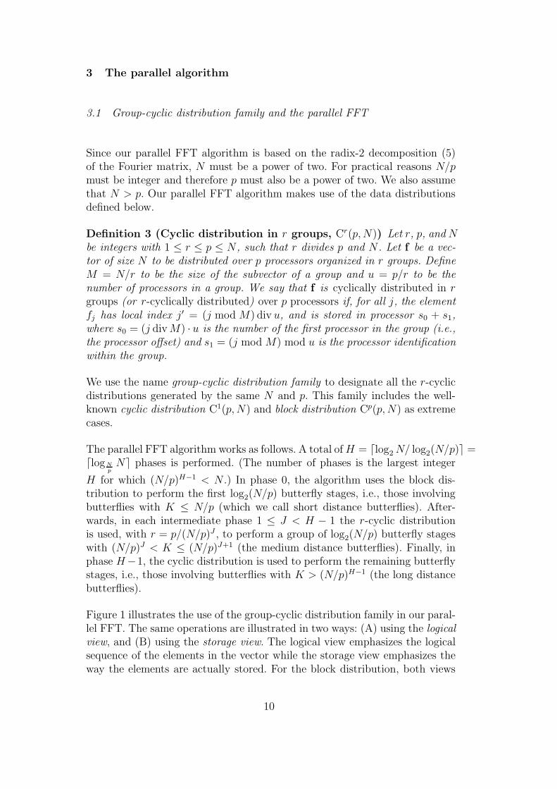
Since our parallel FFT algorithm is based on the radix-2 decomposition (5)of the Fourier matrix, N must be a power of two. For practical reasons N/pmust be integer and therefore p must also be a power of two. We also assumethat N > p. Our parallel FFT algorithm makes use of the data distributionsdefined below.

Definition 3 (Cyclic distribution in r groups, Cr(p, N)) Let r, p, and Nbe integers with 1 ≤ r ≤ p ≤ N , such that r divides p and N . Let f be a vec-tor of size N to be distributed over p processors organized in r groups. DefineM = N/r to be the size of the subvector of a group and u = p/r to be thenumber of processors in a group. We say that f is cyclically distributed in rgroups (or r-cyclically distributed) over p processors if, for all j, the elementfj has local index j′ = (j mod M) div u, and is stored in processor s0 + s1,where s0 = (j div M) · u is the number of the first processor in the group (i.e.,the processor offset) and s1 = (j mod M) mod u is the processor identificationwithin the group.

We use the name group-cyclic distribution family to designate all the r-cyclicdistributions generated by the same N and p. This family includes the well-known cyclic distribution C1(p, N) and block distribution Cp(p, N) as extremecases.

The parallel FFT algorithm works as follows. A total of H = ⌈log2 N/ log2(N/p)⌉ =⌈logN

pN⌉ phases is performed. (The number of phases is the largest integer

H for which (N/p)H−1 < N .) In phase 0, the algorithm uses the block dis-tribution to perform the first log2(N/p) butterfly stages, i.e., those involvingbutterflies with K ≤ N/p (which we call short distance butterflies). After-wards, in each intermediate phase 1 ≤ J < H − 1 the r-cyclic distributionis used, with r = p/(N/p)J , to perform a group of log2(N/p) butterfly stageswith (N/p)J < K ≤ (N/p)J+1 (the medium distance butterflies). Finally, inphase H−1, the cyclic distribution is used to perform the remaining butterflystages, i.e., those involving butterflies with K > (N/p)H−1 (the long distancebutterflies).

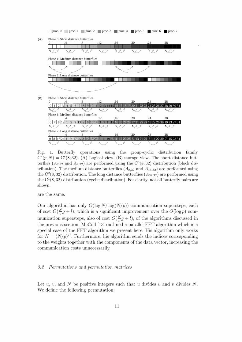
Figure 1 illustrates the use of the group-cyclic distribution family in our paral-lel FFT. The same operations are illustrated in two ways: (A) using the logicalview, and (B) using the storage view. The logical view emphasizes the logicalsequence of the elements in the vector while the storage view emphasizes theway the elements are actually stored. For the block distribution, both views

10

2716 17 25 10 18 26 11 198 1240 3 3112 1320 2128 29 14 22 30 159 4 5 6 72 2328242016128

0 4 81 2 3 5 6 7 1210 11 13 15 16 20 24 2817 18 19 21 22 23 25 26 27 29 30 31

0 4 8 12 16 20 24 281 5 9 2 6 3 70 4 8 12 10 1113 14 15 3119 2716 17 1820 2124 28 25 29 22 26 30

9

40

28242016128414

0

23

(A)0 4 8 12 16 20 24 28

Phase 2: Long distance butterflies

Phase 0: Short distance butterflies

Phase 1: Medium distance butterflies

proc. 6proc. 5 proc. 7proc. 4proc. 0 proc. 1 proc. 2 proc. 3

(B) Phase 0: Short distance butterflies

Phase 1: Medium distance butterflies

Phase 2: Long distance butterflies

.

Fig. 1. Butterfly operations using the group-cyclic distribution familyCr(p,N) = Cr(8, 32). (A) Logical view, (B) storage view. The short distance but-terflies (A2,32 and A4,32) are performed using the C8(8, 32) distribution (block dis-tribution). The medium distance butterflies (A8,32 and A16,32) are performed usingthe C2(8, 32) distribution. The long distance butterflies (A32,32) are performed usingthe C1(8, 32) distribution (cyclic distribution). For clarity, not all butterfly pairs areshown.

are the same.

Our algorithm has only O(logN/ log(N/p)) communication supersteps, eachof cost O(N

pg + l), which is a significant improvement over the O(log p) com-

munication supersteps, also of cost O(Npg + l), of the algorithms discussed in

the previous section. McColl [13] outlined a parallel FFT algorithm which is aspecial case of the FFT algorithm we present here. His algorithm only worksfor N = (N/p)H . Furthermore, his algorithm sends the indices correspondingto the weights together with the components of the data vector, increasing thecommunication costs unnecessarily.

3.2 Permutations and permutation matrices

Let u, v, and N be positive integers such that u divides v and v divides N .We define the following permutation:

11

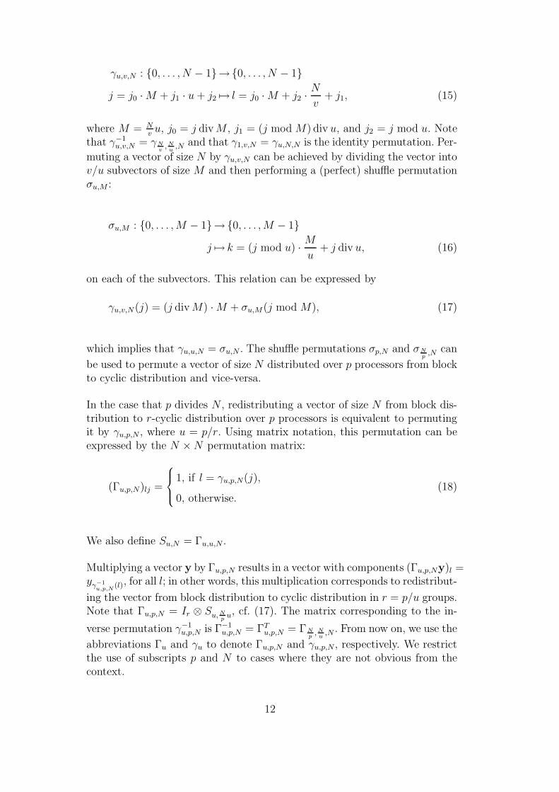
γu,v,N : 0, . . . , N − 1→0, . . . , N − 1

j = j0 ·M + j1 · u + j2 7→ l = j0 ·M + j2 ·N

v+ j1, (15)

where M = Nvu, j0 = j div M , j1 = (j mod M) div u, and j2 = j mod u. Note

that γ−1u,v,N = γN

v, N

u,N and that γ1,v,N = γu,N,N is the identity permutation. Per-

muting a vector of size N by γu,v,N can be achieved by dividing the vector intov/u subvectors of size M and then performing a (perfect) shuffle permutationσu,M :

σu,M : 0, . . . , M − 1→0, . . . , M − 1

j 7→ k = (j mod u) · Mu

+ j div u, (16)

on each of the subvectors. This relation can be expressed by

γu,v,N(j) = (j div M) ·M + σu,M(j mod M), (17)

which implies that γu,u,N = σu,N . The shuffle permutations σp,N and σNp

,N can

be used to permute a vector of size N distributed over p processors from blockto cyclic distribution and vice-versa.

In the case that p divides N , redistributing a vector of size N from block dis-tribution to r-cyclic distribution over p processors is equivalent to permutingit by γu,p,N , where u = p/r. Using matrix notation, this permutation can beexpressed by the N ×N permutation matrix:

(Γu,p,N)lj =

1, if l = γu,p,N(j),

0, otherwise.(18)

We also define Su,N = Γu,u,N .

Multiplying a vector y by Γu,p,N results in a vector with components (Γu,p,Ny)l =yγ−1

u,p,N(l), for all l; in other words, this multiplication corresponds to redistribut-

ing the vector from block distribution to cyclic distribution in r = p/u groups.Note that Γu,p,N = Ir ⊗ Su, N

pu, cf. (17). The matrix corresponding to the in-

verse permutation γ−1u,p,N is Γ−1

u,p,N = ΓTu,p,N = ΓN

p, N

u,N . From now on, we use the

abbreviations Γu and γu to denote Γu,p,N and γu,p,N , respectively. We restrictthe use of subscripts p and N to cases where they are not obvious from thecontext.

12

3.3 Decomposition of the Fourier matrix

To obtain the parallel FFT algorithm, we modify the original radix-2 decom-position of the Fourier matrix (5) by inserting identity permutation matricesIN = Γ−1

u Γu corresponding to the changes of distribution, and regrouping thematrices in the resulting decomposition. In the case that 1 < p ≤

√N and

hence H = 2, this is done as follows:

FN = Γ−1p Γp ·AN,N · Γ−1

p Γp · · ·Γ−1p Γp · A2N

p,N · Γ−1

p Γp · ANp

,N . . . A2,NPN

= Γ−1p (ΓpAN,NΓ−1

p ) · · · (ΓpA2Np

,NΓ−1p )Γp · AN

p,N . . . A2,NPN . (19)

By defining

Ak,u,p,N = Γu,p,NAku,NΓ−1u,p,N (20)

and using the fact that Γ1 is the identity matrix, we can rewrite (19) as

FN = Γ−1p · AN

p,p,p,N · · · A2 N

p2 ,p,p,N︸ ︷︷ ︸

phase 1

·ΓpΓ−11 · AN

p,1,p,N · · · A2,1,p,N

︸ ︷︷ ︸

phase 0

·Γ1PN . (21)

From now on, we denote Ak,u,p,N by Ak,u, reserving the indices p and N forsituations where they are not obvious from the context and for stand-alonedefinitions. In the general case, not restricted to p ≤

√N , we arrive at the

following decomposition of the Fourier matrix:

FN = Γ−1p AN

p,p . . . A

2(N/p)H−1

p,p

︸ ︷︷ ︸

phase H−1

Γp · Γ−1(N

p)H−2 AN

p,(N

p)H−2 . . . A2,(N

p)H−2

︸ ︷︷ ︸

phase H−2

·

Γ(Np

)H−2 · · ·Γ−1Np

ANp

, Np

. . . A2, Np

︸ ︷︷ ︸

phase 1

ΓNp· Γ−1

1 ANp

,1 . . . A2,1︸ ︷︷ ︸

phase 0

Γ1 · PN .(22)

The matrices Ak,u are block diagonal matrices with block size Np:

Ak,u,p,N = Ir ⊗ diag(A0/uk,n , A

1/uk,n , . . . , A

(u−1)/uk,n ), (23)

where r = p/u, n = N/p, and Aαk,n was defined previously, cf. (9). We shall

formally state this as Corollary 5 which follows from Theorem 4. Figure 2exemplifies the structure of the matrix Ak,u.

13

(A)

(C)

(B)

s1 = 0

s1 = 1

s1 = 2

s1 = 3

B0

8

B0

8

B1

4

8

B1

4

8

B2

4

8

B2

4

8

B3

4

8

B3

4

8

A0

8

A

1

4

8

A

2

4

8

A

3

4

8

A0

8

A

1

4

8

A

2

4

8

A

3

4

8

1

1

1

1

w

1

4

8

w

31

4

8

w

11

4

8

w

21

4

8

−w

1

4

8

−w

11

4

8

−w

21

4

8

−w

31

4

8

1

1

1

1

1

1

1

1

1

1

1

1

1

1

1

1

1

1

1

1

1

1

1

1B

3

4

8=B

2

4

8=

B1

4

8=B0

8=

1

1

1

1 w0

8

w1

8

w2

8

w3

8

−w0

8

−w1

8

−w2

8

−w3

8

w

2

4

8

w

12

4

8

w

22

4

8

−w

2

4

8

−w

12

4

8

−w

22

4

8

−w

32

4

8

w

3

4

8

w

13

4

8

w

23

4

8

w

33

4

8

−w

3

4

8

−w

13

4

8

−w

23

4

8

−w

33

4

8

w

32

4

8

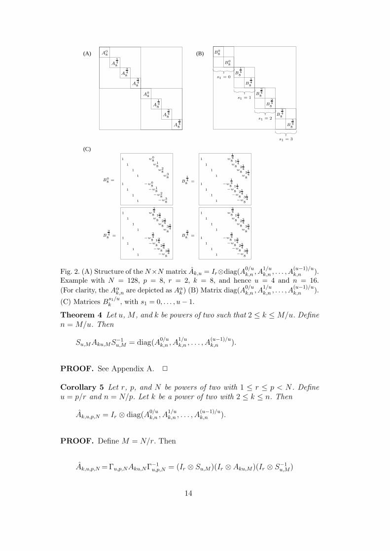
Fig. 2. (A) Structure of the N×N matrix Ak,u = Ir⊗diag(A0/uk,n , A

1/uk,n , . . . , A

(u−1)/uk,n ).

Example with N = 128, p = 8, r = 2, k = 8, and hence u = 4 and n = 16.

(For clarity, the Aαk,n are depicted as Aα

k ) (B) Matrix diag(A0/uk,n , A

1/uk,n , . . . , A

(u−1)/uk,n ).

(C) Matrices Bs1/uk , with s1 = 0, . . . , u− 1.

Theorem 4 Let u, M , and k be powers of two such that 2 ≤ k ≤M/u. Definen = M/u. Then

Su,MAku,MS−1u,M = diag(A

0/uk,n , A

1/uk,n , . . . , A

(u−1)/uk,n ).

PROOF. See Appendix A. 2

Corollary 5 Let r, p, and N be powers of two with 1 ≤ r ≤ p < N . Defineu = p/r and n = N/p. Let k be a power of two with 2 ≤ k ≤ n. Then

Ak,u,p,N = Ir ⊗ diag(A0/uk,n , A

1/uk,n , . . . , A

(u−1)/uk,n ).

PROOF. Define M = N/r. Then

Ak,u,p,N =Γu,p,NAku,NΓ−1u,p,N = (Ir ⊗ Su,M)(Ir ⊗Aku,M)(Ir ⊗ S−1

u,M)

14

= Ir ⊗ (Su,MAku,MS−1u,M) = Ir ⊗ diag(A

0/uk,n , A

1/uk,n , . . . , A

(u−1)/uk,n ).

2

Starting from the Fourier matrix decomposition (22), it is easy to develop aparallel (BSP) FFT algorithm. Since all the matrices Ak,u are block diagonal

matrices with block size equal to N/p, every multiplication Ak,u ·y can be han-dled locally, provided that the vector y is in the block distribution. This prop-erty guarantees that matrix decomposition (22) separates computation andcommunication completely: each generalized butterfly phase (AN

p,u . . . A2,u) ·y

is a computation superstep, whereas each permutation Γu · y is a communi-cation superstep. In the next section we give a complete description of theresulting parallel algorithm.

4 Implementation of the parallel algorithm

We describe our parallel algorithms with a high level of detail. As a result, theyare ready to be implemented, though not necessarily completely optimized.The following list introduces the terminology used in describing our parallelalgorithms.

• Supersteps. Each superstep is numbered textually and labeled accordingto its type: (Comp ) computation superstep, (Comm ) communication super-step, (CpCm ) subroutine containing both computation and communicationsupersteps. Global synchronizations are explicitly indicated by the keywordSynchronize.• Indexing. All the indices of vectors are global. This means that vector

elements have a unique index which is independent of the processor thatowns it. This property enables us to describe variables and gain access tovectors in an unambiguous manner, even though the vector is distributedand each processor has only part of it.• Communication. Communication between processors is indicated using

gj ← Put(pid, n, fi).

This operation puts n elements of vector f , starting from element i, intoprocessor pid and stores them there in vector g starting from element j.Subscripts are not needed when the first element of the vector is 0 or whencommunicating scalars. When communicating more than one element, weuse boldface to emphasize that we are dealing with a vector and not a scalar.All puts are assumed to be buffered, so that they are safely carried out, evenif f and g happen to be the same.

15

Algorithm 2 is a direct implementation of the matrix decomposition (22). Notethat to obtain the normalized inverse transform, the output vector must bedivided by N . The subroutines used in the FFT algorithm are described inthe following subsections.

Algorithm 2 Parallel fast Fourier transform.Call BSP FFT(s, p, sign, N,y).

Input y = (yin0 , . . . , yin

N−1): Complex vector of size N , block distributed overp processors; p and N are powers of two with p < N ; s is the processoridentification number with 0 ≤ s < p; sign is the transform direction.

Output y← (yout0 , . . . , yout

N−1), where youtk =

∑N−1j=0 yin

j exp(sign · 2πijk/N).

1CpCm Parallel bit reversal permutation: y← PN · y.BSP BitRev(s, p, N,y)

2Comp Phase 0, short distance butterflies: y← (ANp

,N . . . A2,N) · y.

BTFLY(0, sign, Np, 4,ysN

p)

3CpCm Permutation to the r-cyclic distribution: y← Γp/r · y,with r = max(1, p/(N/p)).BSP BlockToCyclic(s− s mod N

p, s mod N

p, min(p, N

p), N

p,y(s−s mod N

p)Np)

H ← ⌈logNp

N⌉for J = 1 to H − 2 do

4Comp Phase J , medium distance butterflies: y← (ANp

,(Np

)J . . . A2,(Np

)J ) · y.

BTFLY( s mod (N/p)J

(N/p)J , sign, Np, 4,ysN

p)

5Comm Permutation to the r-cyclic distribution: y← (Γ prΓ−1

(Np

)J ) · y,

with r = max(1, p/(N/p)J+1).BSP CyclicToCyclic(s, p, N, (N/p)J , min(p, (N/p)J+1),y)

6Comp Phase H − 1, long distance butterflies: y← (ANp

,p . . . A2

(N/p)H−1

p,p) · y.

BTFLY( sp, sign, N

p, 4 (N/p)H−1

p,ysN

p)

7CpCm Permutation to block distribution: y← Γ−1p · y.

BSP CyclicToBlock(0, s, p, Np,y)

4.1 Generalized butterflies

The sequential subroutine BTFLY, which multiplies the input vector by Aαn,n . . . Aα

k0,nAαk0/2,n

is described in Algorithm 3.

Algorithm 3 Sequential generalized butterfly operations.

16

Call BTFLY(α, sign, n, k0,y).

Input α: Butterfly parameter, used to compute the correct weights; 0 ≤ α <1.k0: Smaller 4-butterfly size; k0 is a power of two with 4 ≤ k0 ≤ 2n.y = (y0, . . . , yn−1): Complex vector of size n; n is a power of two withn ≥ 2.

Output y← Aαn,n . . . Aα

k0,nAαk0/2,ny for forward (sign = 1), and

y← Aαn,n . . . Aα

k0,nAαk0/2,ny for backward (sign = −1).

Step 1. Perform pairs of butterfly stages Aαk,nA

αk/2,n.

k ← k0

while k ≤ n do

for t = 0 to n− k step k do

Perform 4-butterfly Dαk = Bα

k (I2 ⊗Bαk/2).

for j = 0 to k/4− 1 do

a← yt+j + wsign·2(j+α)k · yt+j+k/4

b← yt+j − wsign·2(j+α)k · yt+j+k/4

c← wsign·(j+α)k · yt+j+k/2 + w

sign·3(j+α)k · yt+j+3k/4

d← wsign·(j+α)k · yt+j+k/2 − w

sign·3(j+α)k · yt+j+3k/4

yt+j ← a + cyt+j+k/4 ← b + sign · diyt+j+k/2 ← a− cyt+j+3k/4 ← b− sign · di

k ← 4 · kStep 2. Perform the last butterfly stage Aα

n,n.if k = 2n then

for j = 0 to n/2− 1 do

a← wsign·(j+α)n · yj+n/2

yj+n/2 ← yj − ayj ← yj + a

If the needed weights are stored in a lookup table, the cost of Algorithm 3 is

CBTFLY(n, k0) =17

4n · log2

4n

k0

+3

4n ·

(

log2

4n

k0

mod 2)

. (24)

The FFT algorithm computes the desired (short, medium, or long distance)butterfly stages corresponding to phase J , 0 ≤ J < H , by defining the inputparameter α = (s mod u)/u, where u = min(p, (N/p)J), and performing thegeneralized butterfly stages on the local part of the vector y (i.e., the subvectorysN

pof size N/p that starts at element sN/p).

17

The total computation cost of our parallel FFT, Algorithm 2, is obtained byadding the costs CBTFLY(N

p, 4) of phases J = 0 to H−2, where H = ⌈logN

pN⌉,

and CBTFLY(Np, 4 (N/p)H−1

p) of the last phase H − 1. (If H = logN

pN , then

(N/p)H−1 = p, and the cost of the last phase is also CBTFLY(Np, 4).) This gives

a total cost of

CFFT,par,Comp(N, p) =17

4

N

plog2 N +

3

4

N

p[(log2

N

pmod 2)⌊logN

pN⌋

+(log2 N mod log2

N

p) mod 2], (25)

where the second term corresponds to the extra cost we have to pay for per-forming 2-butterflies. The communication and synchronization costs of ourparallel FFT are discussed in Section 4.5 after we discuss the parallel permu-tation subroutines.

4.2 Parallel bit reversal

The bit reversal matrix PN is defined by

(PN)jk =

1, if j = revN(k),

0, otherwise.(26)

Here, revN is the bit reversal permutation

revN : 0, . . . , N − 1→0, . . . , N − 1

j =m−1∑

l=0

bl2l 7→ k =

m−1∑

l=0

bm−l−12l, (27)

where m = log2 N and (bm−1 . . . b0)2 is the binary representation of j. Notethat rev−1

N = revN , which means that P−1N = PN .

The bit reversal permutation has the following very useful property.

Lemma 6 Let u = 2q and N = 2m, with q ≤ m. Then

revN (j) = revNu(j div u) +

N

u· revu(j mod u), 0 ≤ j < N.

PROOF. Straightforward. 2

18

Corollary 7 Let u ≤ N be powers of two. Then PN = (Iu⊗PNu)(Pu⊗IN

u)Su,N .

PROOF. The matrix (Iu ⊗ PNu)(Pu ⊗ IN

u)Su,N corresponds to a sequence of

three permutations:

(1) j → l = σu,N (j) = j mod u · Nu

+ j div u;(2) l → t = revu(l div N

u) · N

u+ l mod N

u= revu(j mod u) · N

u+ j div u;

(3) t→ k = t div Nu·N

u+revN

u(t mod N

u) = revu(j mod u)·N

u+revN

u(j div u) =

revN(j).

2

Let y be a vector of size N = 2m block distributed over p = 2q processors.Suppose that we want to permute it by a bit reversal permutation, i.e., performy← PN ·y. Applying Corollary 7 with u = p, it is possible to split the parallelbit reversal permutation into two parts as shown in Algorithm 4. The firstpart sends the elements to the final destination processors, but with the localindices still in the original order:

j → t = revp(j mod p)︸ ︷︷ ︸

Proc(t)

·Np

+ j div p︸ ︷︷ ︸

t′

.

Having as a basis the block distribution, we use from now on Proc(k) = k div Np

to denote the processor in which element k is stored, and k′ = k mod Np

todenote the local index of the element. The second part permutes the localindices t′:

t′ → k′ = revNp(t′).

Algorithm 4 Parallel bit reversal.Call BSP BitRev(s, p, N,y).

Input y = (y0, . . . , yN−1): Complex vector of size N , block distributed over pprocessors; p and N are powers of two with p < N ; s is the processoridentification number with 0 ≤ s < p.

Output y← PNy.

1Comm Global permutation: y← (Pp ⊗ INp)Sp,N · y.

for j = sNp

to sNp

+ Np− 1 do

dest← revp(j mod p)xdest·N

p+j div p ← Put(dest, 1, yj)

19

Synchronize

2Comp Local bit reversal: y← (Ip ⊗ PNp) · y.

for t′ = 0 to Np− 1 do

ys Np

+rev Np

(t′) ← xs Np

+t′

If we combine the local bit reversal (superstep 2 of Algorithm 4) with the shortdistance butterfly phase (superstep 2 of Algorithm 2), we obtain a completelocal sequential FFT. This means that we can easily replace the two superstepsby any optimized FFT subroutine we can lay our hands on. If p < N/p, it ispossible to optimize superstep 1 of Algorithm 4 by sending packets of data.This is done in a similar way as when permuting from block to cyclic distri-bution (see Section 4.4); the only difference is in the destination processor,which is revp(j mod p) instead of j mod p.

4.3 Permutations within the group-cyclic distribution family

Permuting a vector from the Cr1(p, N) distribution to the Cr2(p, N) distribu-tion, where r1 = p/u1 and r2 = p/u2 may be any possible group sizes, notnecessarily powers of two, can be done as follows: first, use γ−1

u1to permute

the vector to the block distribution, and then use γu2 to permute it to theCr2(p, N) distribution. This operation is expensive if performed in parallel,because all the data have to be moved twice around the processors. The bestapproach is to combine the two permutations into one:

γu2u1

: 0, . . . , N − 1→0, . . . , N − 1j 7→ l = γu2(γ

−1u1

(j)). (28)

(Note that (γu2u1

)−1 = γu1u2

, and that γu2u1

is an abbreviation for γu2u1,p,N .) In the

general case, there is no simple formula for computing the destination indexl. Algorithm 5 implements this case.

Algorithm 5 Parallel permutation from r1-cyclic to r2-cyclic distribution.Call BSP CyclicToCyclic(s, p, N, u1, u2,y).

Input y = (y0, . . . , yN−1): Complex vector of size N , block distributed overp processors; s is the processor identification number with 0 ≤ s < p;u1 and u2 are the number of processors in the old group, u1 = p/r1,and in the new group, u2 = p/r2, respectively.

Output y← Γu2Γ−1u1· y.

1Comm Global permutation γu2u1

.

20

for j = sNp

to sNp

+ Np− 1 do

l ← γu2u1

(j)yl ← Put(l div N

p, 1, yj)

Synchronize

Some combinations of the parameters r1, r2, p, and N , however, lead to simplerexpressions for the destination index. The simplest case is when r1 or r2 isequal to p, i.e., one of the distributions involved is the block distribution. Thissituation occurs in supersteps 3 and 7 of the FFT algorithm and is discussedin Section 4.4.

4.4 Permutation from block to cyclic distribution

The permutations σp,N and σ−1p,N are the permutations that convert a vector

from block to cyclic distribution and vice versa. In the case that p < N/p,both σp,N and σ−1

p,N can be optimized by sending packets of size N/p2, wherewe assume that p2 divides N .

For σp,N , this is done as follows. Let b = N/p. First, we perform a localpermutation σp,b on the local index j′,

j′ → t′ = j′ mod p · bp

+ j′ div p.

Then we perform a global cyclic permutation of packets on the global indext = t0 · b + t1 · b

p+ t2,

t→ k = t1︸︷︷︸

Proc(k)

·b + t0 ·b

p+ t2

︸ ︷︷ ︸

k′

. (29)

This method is illustrated in Figure 3. To verify that it indeed achieves thedesired permutation, we substitute t0 = j div b, t1 = (j mod b) mod p, andt2 = (j mod b) div p into (29), obtaining

k =(j mod b) mod p · b + j div b · bp

+ (j mod b) div p

= j mod p · b + (j div b · b + j mod b) div p

= j mod p · b + j div p

=σp,N(j).

21

8 1413121110 15

18 27 3116 20 17 21 19 23 24 28 25 29 26 300 4 91 5 3 72 6 8 12 13 10 14 11 150 8 16 24

0 8 16 24

302927 28259654321 247 310 16 222120191817 23241680

proc. 3proc. 2proc. 1

3 7 11 15 19 23 27 312 10 14 22 26 306 18

(A)

26

proc. 0

22

(B)

0 4 8 12 2816 20 24 1 5 9 13 17 21 25 29

Fig. 3. Two-stage permutation from block to cyclic distribution (storage view).Example with N = 32 and p = 4. (A) Local σ4,8 permutation. (B) Global cyclicpermutation of packets of size 2.

Algorithm 6 uses the idea described above to permute from block to cyclicdistribution within a group of u processors, numbered s0, s0 +1, . . . , s0 +u−1.The corresponding subroutine is called with u = min(p, N/p) in superstep 3of the FFT algorithm, where it performs the permutation for all the p/u = rgroups simultaneously. This achieves the desired permutation by γu,p,N , be-cause permuting a vector of size N by γu,p,N is the same as dividing it into rsubvectors of size M = N/r and then performing a shuffle permutation σu,M

on each of the subvectors, cf. (17).

Algorithm 6 Parallel permutation from block to cyclic distribution within agroup of processors.Call BSP BlockToCyclic(s0, s1, u, b,y).

Input s0, s1: Processor offset and processor identification within group; 0 ≤s1 < u.y = (y0, . . . , yub−1): Complex vector of size ub, block distributed withina group of u processors; the local block size, b, is a multiple of u, ifu < b.

Output y← Su,uby.

if u ≥ b then

1Comm Global σu,ub permutation.for j = s1 · b to (s1 + 1) · b− 1 do

yσu,ub(j) ← Put(s0 + j mod u, 1, yj)Synchronize

else

2Comp Local σu,b permutation.for j′ = 0 to b− 1 do

xs1·b+σu,b(j′) ← ys1·b+j′

3Comm Global cyclic permutation of packets.for proc = 0 to u− 1 do

22

yproc·b+s1·bu← Put(s0 + proc, b

u, xs1·b+proc· b

u)

Synchronize

Subroutine BSP CyclicToBlock, which carries out γ−1u,p,N is obtained by in-

verting subroutine BSP BlockToCyclic. The algorithm starts by performing aglobal cyclic permutation of packets within a group of u processors, and thenit carries out a local permutation σ−1

u,b. (The algorithm is not presented here;see [15] for more details.)

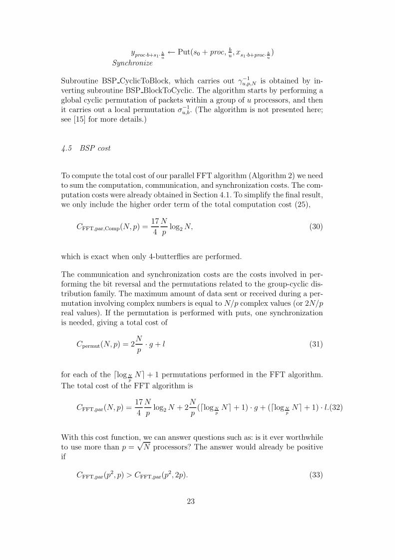
4.5 BSP cost

To compute the total cost of our parallel FFT algorithm (Algorithm 2) we needto sum the computation, communication, and synchronization costs. The com-putation costs were already obtained in Section 4.1. To simplify the final result,we only include the higher order term of the total computation cost (25),

CFFT,par,Comp(N, p) =17

4

N

plog2 N, (30)

which is exact when only 4-butterflies are performed.

The communication and synchronization costs are the costs involved in per-forming the bit reversal and the permutations related to the group-cyclic dis-tribution family. The maximum amount of data sent or received during a per-mutation involving complex numbers is equal to N/p complex values (or 2N/preal values). If the permutation is performed with puts, one synchronizationis needed, giving a total cost of

Cpermut(N, p) = 2N

p· g + l (31)

for each of the ⌈logNp

N⌉ + 1 permutations performed in the FFT algorithm.

The total cost of the FFT algorithm is

CFFT,par(N, p) =17

4

N

plog2 N + 2

N

p(⌈logN

pN⌉+ 1) · g + (⌈logN

pN⌉+ 1) · l.(32)

With this cost function, we can answer questions such as: is it ever worthwhileto use more than p =

√N processors? The answer would already be positive

if

CFFT,par(p2, p) > CFFT,par(p

2, 2p). (33)

23

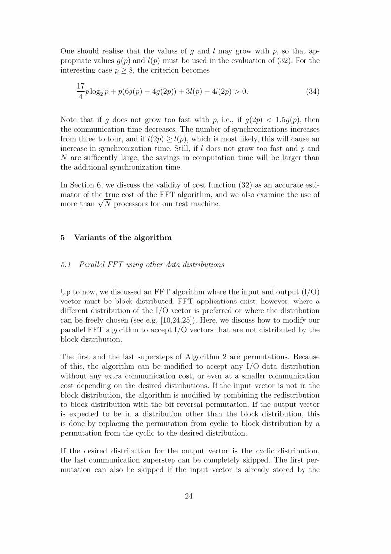
One should realise that the values of g and l may grow with p, so that ap-propriate values g(p) and l(p) must be used in the evaluation of (32). For theinteresting case p ≥ 8, the criterion becomes

17

4p log2 p + p(6g(p)− 4g(2p)) + 3l(p)− 4l(2p) > 0. (34)

Note that if g does not grow too fast with p, i.e., if g(2p) < 1.5g(p), thenthe communication time decreases. The number of synchronizations increasesfrom three to four, and if l(2p) ≥ l(p), which is most likely, this will cause anincrease in synchronization time. Still, if l does not grow too fast and p andN are sufficently large, the savings in computation time will be larger thanthe additional synchronization time.

In Section 6, we discuss the validity of cost function (32) as an accurate esti-mator of the true cost of the FFT algorithm, and we also examine the use ofmore than

√N processors for our test machine.

5 Variants of the algorithm

5.1 Parallel FFT using other data distributions

Up to now, we discussed an FFT algorithm where the input and output (I/O)vector must be block distributed. FFT applications exist, however, where adifferent distribution of the I/O vector is preferred or where the distributioncan be freely chosen (see e.g. [10,24,25]). Here, we discuss how to modify ourparallel FFT algorithm to accept I/O vectors that are not distributed by theblock distribution.

The first and the last supersteps of Algorithm 2 are permutations. Becauseof this, the algorithm can be modified to accept any I/O data distributionwithout any extra communication cost, or even at a smaller communicationcost depending on the desired distributions. If the input vector is not in theblock distribution, the algorithm is modified by combining the redistributionto block distribution with the bit reversal permutation. If the output vectoris expected to be in a distribution other than the block distribution, thisis done by replacing the permutation from cyclic to block distribution by apermutation from the cyclic to the desired distribution.

If the desired distribution for the output vector is the cyclic distribution,the last communication superstep can be completely skipped. The first per-mutation can also be skipped if the input vector is already stored by the

24

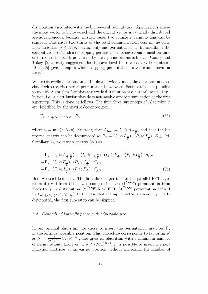
distribution associated with the bit reversal permutation. Applications wherethe input vector is bit reversed and the output vector is cyclically distributedare advantageous, because, in such cases, two complete permutations can beskipped. This saves two thirds of the total communication cost in the com-mon case that p ≤ N/p, leaving only one permutation in the middle of thecomputation. (The idea of skipping permutations to save communication timeor to reduce the overhead caused by local permutations is known. Cooley andTukey [2] already suggested this to save local bit reversals. Other authors[10,24,25] give examples where skipping permutations saves communicationtime.)

While the cyclic distribution is simple and widely used, the distribution asso-ciated with the bit reversal permutation is awkward. Fortunately, it is possibleto modify Algorithm 2 so that the cyclic distribution is a natural input distri-bution, i.e., a distribution that does not involve any communication as the firstsuperstep. This is done as follows. The first three supersteps of Algorithm 2are described by the matrix decomposition

Γu · ANp

,N . . . A2,N · PN , (35)

where u = min(p, N/p). Knowing that AK,N = Ip ⊗ AK, Np, and that the bit

reversal matrix can be decomposed as PN = (Ip ⊗ PNp) · (Pp ⊗ IN

p) · Sp,N (cf.

Corollary 7), we rewrite matrix (35) as

Γu · (Ip ⊗ ANp

, Np) . . . (Ip ⊗A2, N

p) · (Ip ⊗ PN

p) · (Pp ⊗ IN

p) · Sp,N

=Γu · (Ip ⊗ FNp) · (Pp ⊗ IN

p) · Sp,N

=Γu · (Pp ⊗ INp) · (Ip ⊗ FN

p) · Sp,N . (36)

Here we used Lemma 2. The first three supersteps of the parallel FFT algo-rithm derived from this new decomposition are: (1Comm) permutation from

block to cyclic distribution, (2Comp) local FFT, (3Comm) permutation definedby Γmin(p,N/p) · (Pp⊗IN

p). In the case that the input vector is already cyclically

distributed, the first superstep can be skipped.

5.2 Generalized butterfly phase with adjustable size

In our original algorithm, we chose to insert the permutation matrices Γu

in the leftmost possible position. This procedure corresponds to factoring Nas N = N

(N/p)H−1 (N/p)H−1, and gives an algorithm with a minimum number

of permutations. However, if p 6= (N/p)H−1, it is possible to insert the per-mutation matrices at an earlier position without increasing the number of

25

permutations. The resulting algorithm corresponds to a different factorizationof N .

We can use this flexibility to reduce the computation cost of some combina-tions of p and N by inserting the permutations so that a maximal numberof generalized butterfly stages are paired off. Another reason to permute thevector at an earlier stage is that the sizes of the butterfly phases can be betterbalanced (so that all factors of N have approximately the same size). Thiswould enhance the performance on a cache-sensitive computer (see the discus-sion in Section 6). An even more effective way of enhancing the performance ona cache-sensitive computer is to reduce the butterfly sizes so that the butter-flies always fit completely in the cache. We suggest a method in the followingsubsection.

5.3 Cache-friendly parallel FFT

Each computation superstep of our parallel FFT algorithm performs a but-terfly phase which consists of a sequence of generalized butterfly stages rep-resented by the operation y ← Rα

l,ny, where l and n are powers of two with2 ≤ l ≤ n, and

Rαl,n = Aα

n,n · · ·Aα2l,nAα

l,n, (37)

is an n×n matrix. Suppose that the cache memory of a computer is such thatthe data needed by a butterfly phase of size n/v, where v < n is a power oftwo, fits totally in the computer cache. We can view v as the number of virtualprocessors available in each processor. If we decompose (37) into a sequenceof smaller butterfly phases of size less than or equal to n/v which can becarried out independently from each other, we can fully exploit the cache ofthe computer.

Define h = ⌈lognvn⌉ and j = ⌈logn

vl⌉ − 1, so that (n

v)j < l ≤ (n

v)j+1. Similarly

to (22), if we denote Γu,v,n by Γu, we can write

Rαl,n = Γ−1

v Aαnv

,v . . . Aα

2(n/v)h−1

v,v

︸ ︷︷ ︸

phase h−j−1

Γv · Γ−1(n

v)h−2 Aα

nv

,(nv)h−2 . . . Aα

2,(nv)h−2

︸ ︷︷ ︸

phase h−j−2

Γ(nv)h−2 · . . .

. . . · Γ−1(n

v)j+1 Aα

nv

,(nv)j+1 . . . Aα

2,(nv)j+1

︸ ︷︷ ︸

phase 1

Γ(nv)j+1 · Γ−1

(nv)j Aα

nv

,(nv)j . . . Aα

l

(n/v)j,(n

v)j

︸ ︷︷ ︸

phase 0

Γ(nv)j ,

(38)

26

where Aαk,u is an abbreviation for the n× n matrix Aα

k,u,v,n = Γu,v,nAαku,nΓ

−1u,v,n.

Generalized versions of Theorem 4 and Corollary 5 can be used to prove that

Aαk,u,v,n = I v

u⊗ diag(A

α/uk, n

v, A

(α+1)/uk, n

v, . . . , A

(α+u−1)/uk, n

v). (39)

The matrix decomposition (38) can be used to construct an alternative (cache-friendly) algorithm for the computation of the generalized butterfly phases.Note that if α = 0 then the resulting algorithm can be used to construct acache-friendly sequential FFT algorithm.

6 Performance results and discussion

In this section, we present results on the performance of our implementationof the FFT. We implemented the FFT algorithm for the block distribution inANSI C using the BSPlib communications library [21]. Our programs are com-pletely self-contained, and we did not rely on any system-provided numericalsoftware such as BLAS, FFTs, etc.

We tested our implementation on a Cray T3E with up to 64 processors, eachhaving a theoretical peak speed of 600 Mflop/s. The accuracy of double pre-cision (64-bit) arithmetic is 1.0 × 10−15. We also give accuracy results fromcalculations on a Sun workstation using IEEE 754 floating point arithmetic,which has a double precision accuracy of 2.2 × 10−16, and which is the stan-dard used in many computers such as workstations. To make a consistentcomparison of the results, we compiled all test programs using the bspfront

driver with options -O3 -flibrary-level 2 -fcombine-puts and measuredthe elapsed execution times on exclusively dedicated CPUs using the systemclock. The times given correspond to an average of the execution times of aforward FFT and a normalized backward FFT.

6.1 Accuracy

We tested the overall accuracy of our implementation by measuring the errorobtained when transforming a random complex vector f with values Re(fj) andIm(fj) uniformly distributed between 0 and 1. The relative error is defined as||F∗−F||2/||F||2, where F∗ is the vector obtained by transforming the originalvector f by a forward (or backward) FFT, and F is the exact transform, whichwe computed using the same algorithm but using quadruple precision. Here,|| · ||2 indicates the L2-norm.

27

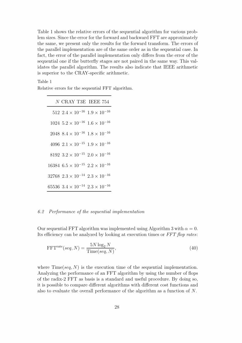
Table 1 shows the relative errors of the sequential algorithm for various prob-lem sizes. Since the error for the forward and backward FFT are approximatelythe same, we present only the results for the forward transform. The errors ofthe parallel implementation are of the same order as in the sequential case. Infact, the error of the parallel implementation only differs from the error of thesequential one if the butterfly stages are not paired in the same way. This val-idates the parallel algorithm. The results also indicate that IEEE arithmeticis superior to the CRAY-specific arithmetic.

Table 1

Relative errors for the sequential FFT algorithm.

N CRAY T3E IEEE 754

512 2.4× 10−16 1.9× 10−16

1024 5.2× 10−16 1.6× 10−16

2048 8.4× 10−16 1.8× 10−16

4096 2.1× 10−15 1.9× 10−16

8192 3.2× 10−15 2.0× 10−16

16384 6.5× 10−15 2.2× 10−16

32768 2.3× 10−14 2.3× 10−16

65536 3.4× 10−14 2.3× 10−16

6.2 Performance of the sequential implementation

Our sequential FFT algorithm was implemented using Algorithm 3 with α = 0.Its efficiency can be analyzed by looking at execution times or FFT flop rates :

FFTrate(seq, N) =5N log2 N

Time(seq, N), (40)

where Time(seq, N) is the execution time of the sequential implementation.Analyzing the performance of an FFT algorithm by using the number of flopsof the radix-2 FFT as basis is a standard and useful procedure. By doing so,it is possible to compare different algorithms with different cost functions andalso to evaluate the overall performance of the algorithm as a function of N .

28

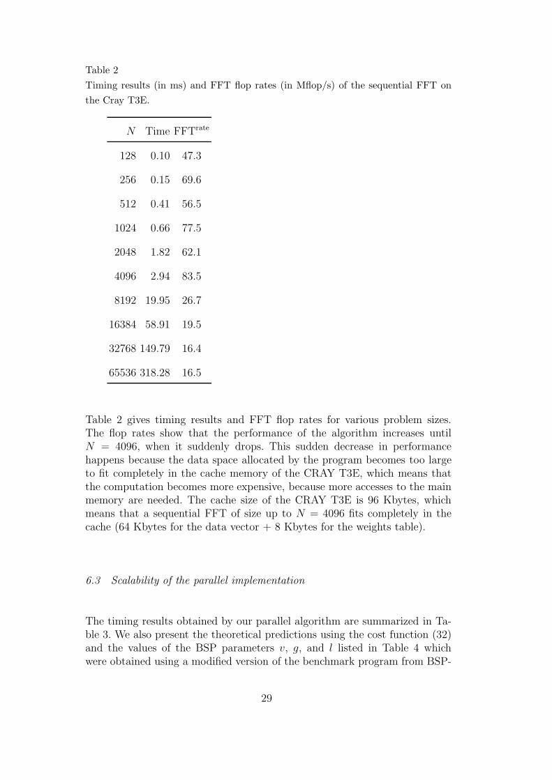
Table 2

Timing results (in ms) and FFT flop rates (in Mflop/s) of the sequential FFT on

the Cray T3E.

N Time FFTrate

128 0.10 47.3

256 0.15 69.6

512 0.41 56.5

1024 0.66 77.5

2048 1.82 62.1

4096 2.94 83.5

8192 19.95 26.7

16384 58.91 19.5

32768 149.79 16.4

65536 318.28 16.5

Table 2 gives timing results and FFT flop rates for various problem sizes.The flop rates show that the performance of the algorithm increases untilN = 4096, when it suddenly drops. This sudden decrease in performancehappens because the data space allocated by the program becomes too largeto fit completely in the cache memory of the CRAY T3E, which means thatthe computation becomes more expensive, because more accesses to the mainmemory are needed. The cache size of the CRAY T3E is 96 Kbytes, whichmeans that a sequential FFT of size up to N = 4096 fits completely in thecache (64 Kbytes for the data vector + 8 Kbytes for the weights table).

6.3 Scalability of the parallel implementation

The timing results obtained by our parallel algorithm are summarized in Ta-ble 3. We also present the theoretical predictions using the cost function (32)and the values of the BSP parameters v, g, and l listed in Table 4 whichwere obtained using a modified version of the benchmark program from BSP-

29

pack 3 [15].

Except for the out-of-cache computations (boldface entries in Table 3), thetimings show that the BSP cost function predicts the behavior of the parallelimplementation well. The discrepancy between predicted and measured resultsfor out-of-cache computations is to be expected, since the computation speed,which we assumed to be constant, suddenly drops when the computationscannot be done completely in cache. These results show that the BSP modelis a valid tool for analyzing and predicting parallel performance.

Table 3 shows that using√

N processors or more is not advantageous on ourtest machine and with our limited number of processors, cf. the timings forN = 512, 1024 with p = 32, 64 and for N = 2048, 4096 with p = 64. Table 4tells us that the growth of g satisfies g(2p) < 1.5g(p) for all p, so that thecommunication time decreases with p for all problem sizes N , cf. (34). Forsmall problems, the increase in synchronization time dominates the decreasein computation and communication time. For larger problem sizes and a largernumber of processors, we expect this to be the reverse, but we do not haveenough processors available to observe this phenomenon.

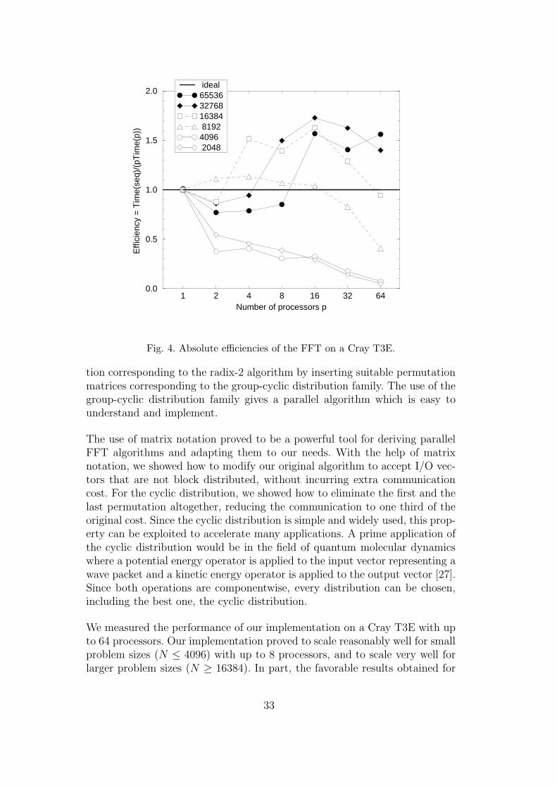
A way of analyzing the scalability of a parallel implementation is to look atits absolute efficiency

Eabs(p, N) =Time(seq, N)

pTime(p, N), (41)

as done in Figure 4. In theory, Eabs(p, N) ≤ 1, and our goal is to achieveefficiencies as close to one as possible. The figure shows moderate efficienciesfor small problem sizes (N ≤ 4096). For N ≥ 8192, efficiencies above one areachieved. Such amazing efficiencies are possible because of the so-called cacheeffect : when N ≥ 8192 the total amount of memory needed by the FFT istoo large to fit in the cache memory of one processor, but, if the problem isexecuted using a sufficiently large number of processors, the memory requiredby each processor becomes small enough to fit in the cache. This effect iswelcome, but it masks the real scalability of the algorithm.

Note that there is a sudden rise in the flop rate when the local problem sizebecomes small enough to fit in the cache. In this way the cache effect canbe easily spotted and the scalability of the algorithm better judged. FFTsizes that fit completely in the cache (N ≤ 4096) have a completely differ-ent behavior than larger problems. For small sizes (N ≤ 4096) the efficiencydecreases notably in going from one to two processors, then it is more orless constant up to 8–16 processors and after that it decreases steadily. For

3 Available at http://www.math.uu.nl/people/bisseling/software.html

30

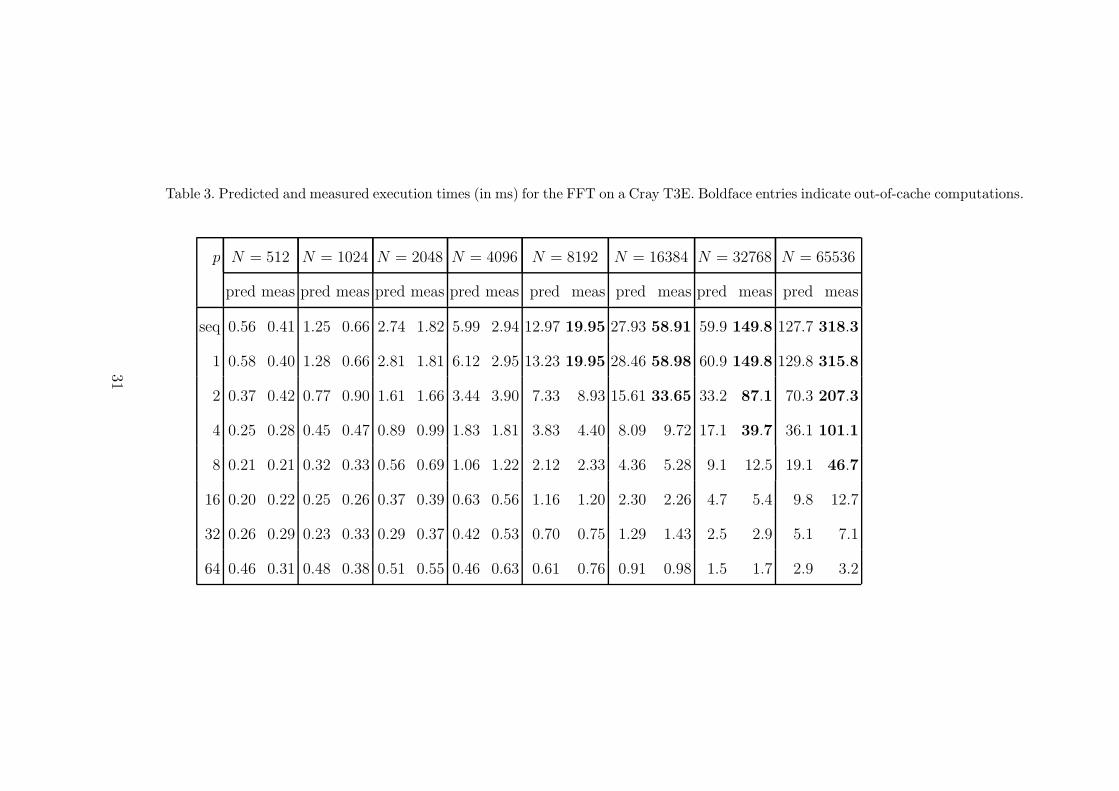
Table 3. Predicted and measured execution times (in ms) for the FFT on a Cray T3E. Boldface entries indicate out-of-cache computations.

p N = 512 N = 1024 N = 2048 N = 4096 N = 8192 N = 16384 N = 32768 N = 65536

pred meas pred meas pred meas pred meas pred meas pred meas pred meas pred meas

seq 0.56 0.41 1.25 0.66 2.74 1.82 5.99 2.94 12.97 19.95 27.93 58.91 59.9 149.8 127.7 318.3

1 0.58 0.40 1.28 0.66 2.81 1.81 6.12 2.95 13.23 19.95 28.46 58.98 60.9 149.8 129.8 315.8

2 0.37 0.42 0.77 0.90 1.61 1.66 3.44 3.90 7.33 8.93 15.61 33.65 33.2 87.1 70.3 207.3

4 0.25 0.28 0.45 0.47 0.89 0.99 1.83 1.81 3.83 4.40 8.09 9.72 17.1 39.7 36.1 101.1

8 0.21 0.21 0.32 0.33 0.56 0.69 1.06 1.22 2.12 2.33 4.36 5.28 9.1 12.5 19.1 46.7

16 0.20 0.22 0.25 0.26 0.37 0.39 0.63 0.56 1.16 1.20 2.30 2.26 4.7 5.4 9.8 12.7

32 0.26 0.29 0.23 0.33 0.29 0.37 0.42 0.53 0.70 0.75 1.29 1.43 2.5 2.9 5.1 7.1

64 0.46 0.31 0.48 0.38 0.51 0.55 0.46 0.63 0.61 0.76 0.91 0.98 1.5 1.7 2.9 3.2

31

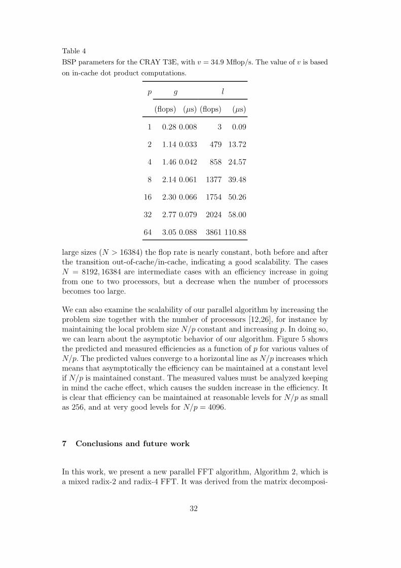
Table 4

BSP parameters for the CRAY T3E, with v = 34.9 Mflop/s. The value of v is based

on in-cache dot product computations.

p g l

(flops) (µs) (flops) (µs)

1 0.28 0.008 3 0.09

2 1.14 0.033 479 13.72

4 1.46 0.042 858 24.57

8 2.14 0.061 1377 39.48

16 2.30 0.066 1754 50.26

32 2.77 0.079 2024 58.00

64 3.05 0.088 3861 110.88

large sizes (N > 16384) the flop rate is nearly constant, both before and afterthe transition out-of-cache/in-cache, indicating a good scalability. The casesN = 8192, 16384 are intermediate cases with an efficiency increase in goingfrom one to two processors, but a decrease when the number of processorsbecomes too large.

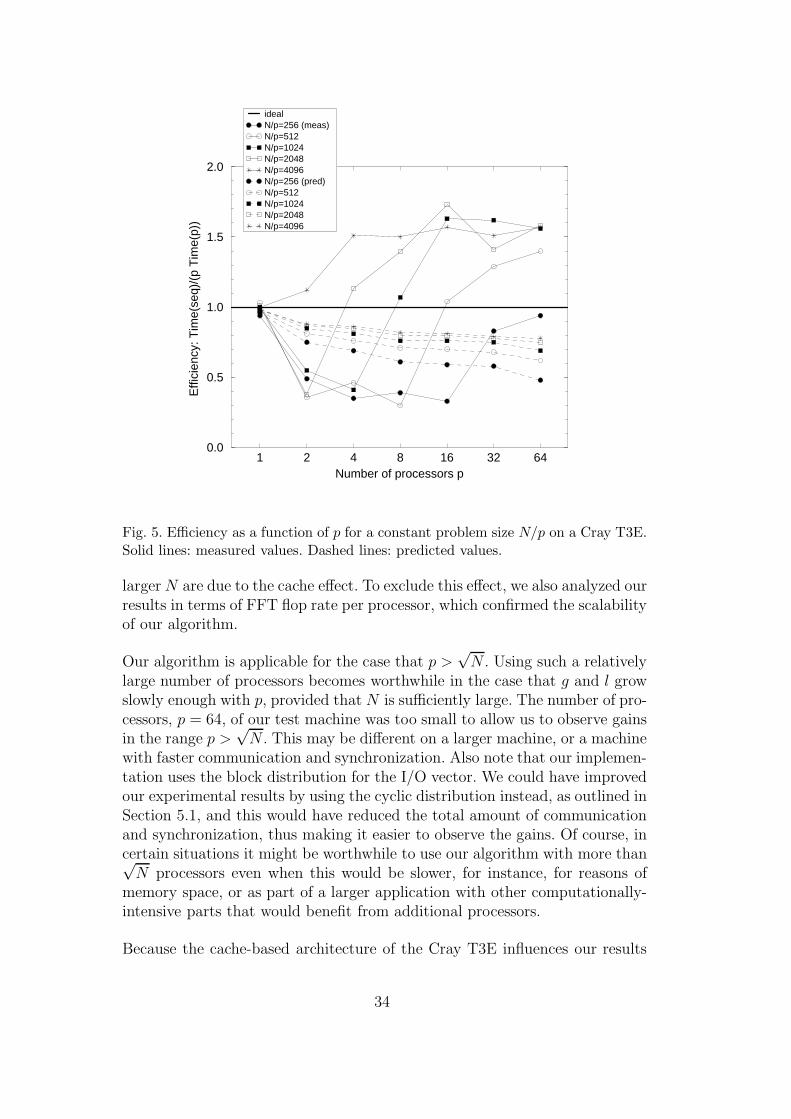
We can also examine the scalability of our parallel algorithm by increasing theproblem size together with the number of processors [12,26], for instance bymaintaining the local problem size N/p constant and increasing p. In doing so,we can learn about the asymptotic behavior of our algorithm. Figure 5 showsthe predicted and measured efficiencies as a function of p for various values ofN/p. The predicted values converge to a horizontal line as N/p increases whichmeans that asymptotically the efficiency can be maintained at a constant levelif N/p is maintained constant. The measured values must be analyzed keepingin mind the cache effect, which causes the sudden increase in the efficiency. Itis clear that efficiency can be maintained at reasonable levels for N/p as smallas 256, and at very good levels for N/p = 4096.

7 Conclusions and future work

In this work, we present a new parallel FFT algorithm, Algorithm 2, which isa mixed radix-2 and radix-4 FFT. It was derived from the matrix decomposi-

32

1 2 4 8 16 32 64Number of processors p

0.0

0.5

1.0

1.5

2.0

Effi

cien

cy =

Tim

e(se

q)/(

pTim

e(p)

)

ideal655363276816384 81924096 2048

Fig. 4. Absolute efficiencies of the FFT on a Cray T3E.

tion corresponding to the radix-2 algorithm by inserting suitable permutationmatrices corresponding to the group-cyclic distribution family. The use of thegroup-cyclic distribution family gives a parallel algorithm which is easy tounderstand and implement.

The use of matrix notation proved to be a powerful tool for deriving parallelFFT algorithms and adapting them to our needs. With the help of matrixnotation, we showed how to modify our original algorithm to accept I/O vec-tors that are not block distributed, without incurring extra communicationcost. For the cyclic distribution, we showed how to eliminate the first and thelast permutation altogether, reducing the communication to one third of theoriginal cost. Since the cyclic distribution is simple and widely used, this prop-erty can be exploited to accelerate many applications. A prime application ofthe cyclic distribution would be in the field of quantum molecular dynamicswhere a potential energy operator is applied to the input vector representing awave packet and a kinetic energy operator is applied to the output vector [27].Since both operations are componentwise, every distribution can be chosen,including the best one, the cyclic distribution.

We measured the performance of our implementation on a Cray T3E with upto 64 processors. Our implementation proved to scale reasonably well for smallproblem sizes (N ≤ 4096) with up to 8 processors, and to scale very well forlarger problem sizes (N ≥ 16384). In part, the favorable results obtained for

33

2 4 8 16 32 641Number of processors p

0.0

0.5

1.0

1.5

2.0

Effi

cien

cy: T

ime(

seq)

/(p

Tim

e(p)

)

idealN/p=256 (meas)N/p=512N/p=1024N/p=2048N/p=4096N/p=256 (pred)N/p=512N/p=1024N/p=2048N/p=4096

Fig. 5. Efficiency as a function of p for a constant problem size N/p on a Cray T3E.Solid lines: measured values. Dashed lines: predicted values.

larger N are due to the cache effect. To exclude this effect, we also analyzed ourresults in terms of FFT flop rate per processor, which confirmed the scalabilityof our algorithm.

Our algorithm is applicable for the case that p >√

N . Using such a relativelylarge number of processors becomes worthwhile in the case that g and l growslowly enough with p, provided that N is sufficiently large. The number of pro-cessors, p = 64, of our test machine was too small to allow us to observe gainsin the range p >

√N . This may be different on a larger machine, or a machine

with faster communication and synchronization. Also note that our implemen-tation uses the block distribution for the I/O vector. We could have improvedour experimental results by using the cyclic distribution instead, as outlined inSection 5.1, and this would have reduced the total amount of communicationand synchronization, thus making it easier to observe the gains. Of course, incertain situations it might be worthwhile to use our algorithm with more than√

N processors even when this would be slower, for instance, for reasons ofmemory space, or as part of a larger application with other computationally-intensive parts that would benefit from additional processors.

Because the cache-based architecture of the Cray T3E influences our results

34

so much, and many other computers have a similar architecture, we proposedthe use of cache-friendly FFT algorithms. A cache-friendly sequential algo-rithm can be derived from our parallel algorithm by replacing the processorsby virtual processors. It is also possible to derive a cache-friendly parallel al-gorithm by writing each generalized butterfly phase as a sequence of smallergeneralized butterfly phases. We expect such an algorithm to scale just as wellas the algorithm we implemented.

A Proof of Theorem 4

The proof uses the following lemma.

Lemma 8 Let u, M , and k be powers of two such that 2 ≤ k ≤M/u. DefineK = ku. Let j be an index, 0 ≤ j < M . Then

(1) If j mod K < K/2, then σu,M(j) mod k < k/2.(2) If j + K/2 < M , then σu,M(j + K/2) = σu,M(j) + k/2.(3) If j1 = j mod M

u, and j0 = j div M

u, then

σ−1u,M(j) mod K

K=

j1 mod k + j0/u

k.

PROOF. Part 1: σu,M(j) mod k = (j mod u·Mu

+j div u) mod k = (j div u) mod k.Now, j div u = (j div K ·K + j mod K) div u = j div K · k + (j mod K) div u.As a consequence, σu,M(j) mod k = (j mod K) div u < (K/2) div u = k/2.

Part 2: σu,M(j + K/2) = (j + K/2) mod u · Mu

+ (j + K/2) div u = j mod u ·Mu

+ j div u + k/2 = σu,M(j) + k/2.

Part 3: σ−1u,M(j) mod K = (j mod M

u·u+j div M

u) mod K = (j1 · u + j0) mod K

= (j1 div k · K + j1 mod k · u + j0) mod K = j1 mod k · u + j0, which gives(σ−1

u,M(j) mod K)/K = (j1 mod k · u + j0)/K = (j1 mod k + j0/u)/k.

2

Proof of Theorem 4.

PROOF. Define K = ku. To prove the theorem, it is sufficient to prove that

Su,MAK,MS−1u,My = diag(A

0/uk,n , . . . , A

(u−1)/uk,n )y, for all y.

35

First note that the vector AK,Mx can be described by

(AK,Mx)j = xj + wj mod KK xj+K/2,

(AK,Mx)j+K/2 = xj − wj mod KK xj+K/2, 0 ≤ j mod K < K/2.

(A.1)

Let x = S−1u,My and z = Su,M(AK,Mx), and substitute xj = yσu,M (j) and

zσu,M (j) = (AK,Mx)j into (A.1). This gives

zσu,M (j) = yσu,M (j) + wj mod KK yσu,M (j+K/2),

zσu,M (j+K/2) = yσu,M (j) − wj mod KK yσu,M (j+K/2), 0 ≤ j mod K < K/2.

(A.2)

Defining l = σu,M(j) and applying Lemma 8 to j gives the following. Part 1 ofLemma 8 says that j mod K < K/2 implies l mod k < k/2. Furthermore, byPart 2, σu,M(j +K/2) = l+k/2. Finally, applying Part 3 to l gives wj mod K

K =

wσ−1

u,M (l) mod K

K = wu(l′ mod k)+s1

K = wl′ mod k+s1/uk , where l′ = l mod n and s1 =

l div n.

Substituting the above results into (A.2) gives the following description ofvector z = Su,MAK,MS−1

u,My:

zl = yl + wl′ mod k+s1/uk yl+k/2,

zl+k/2 = yl − wl′ mod k+s1/uk yl+k/2, 0 ≤ l mod k < k/2.

(A.3)

Writing the index l = s1 · n + (l′ div k) · k + l′ mod k, it is easy to see that

zl = (diag(A0/uk,n , A

1/uk,n , . . . , A

(u−1)/uk,n ) · y)l. The corresponding matrix structure

is illustrated in Figure 2(B). 2

References

[1] W. L. Briggs, V. E. Henson, The DFT: An Owner’s Manual for the DiscreteFourier Transform, SIAM, Philadelphia, PA, 1995.

[2] J. W. Cooley, J. W. Tukey, An algorithm for the machine calculation of complexFourier series, Mathematics of Computation 19 (1965) 297–301.

[3] C. Van Loan, Computational Frameworks for the Fast Fourier Transform,SIAM, Philadelphia, PA, 1992.

[4] R. C. Agarwal, J. W. Cooley, Vectorized mixed radix discrete Fourier transformalgorithms, Proceedings of the IEEE 75 (9) (1987) 1283–1292.

36

[5] M. Ashworth, A. G. Lyne, A segmented FFT algorithm for vector computers,Parallel Computing 6 (1988) 217–224.

[6] A. Averbuch, E. Gabber, B. Gordissky, Y. Medan, A parallel FFT on an MIMDmachine, Parallel Computing 15 (1990) 61–74.

[7] E. Chu, A. George, FFT algorithms and their adaptation to parallel processing,Linear Algebra and its Applications 284 (1998) 95–124.

[8] A. Dubey, M. Zubair, C. E. Grosch, A general purpose subroutine forFast Fourier Transform on a distributed memory parallel machine, ParallelComputing 20 (1994) 1697–1710.

[9] A. Gupta, V. Kumar, The scalability of FFT on parallel computers, IEEETransactions on Parallel and Distributed Systems 4 (8) (1993) 922–932.

[10] O. Haan, A parallel one-dimensional FFT for Cray T3E, in: H. Lederer,F. Hertweck (Eds.), Proceedings of the Fourth European SGI/Cray MPPWorkshop, IPP, Garching, Germany, 1998, pp. 188–198.

[11] M. Hegland, Real and complex fast Fourier transforms on the Fujitsu VPP 500,Parallel Computing 22 (1996) 539–553.

[12] V. Kumar, A. Grama, A. Gupta, G. Karypis, Introduction to ParallelComputing: Design and Analysis of Algorithms, The Benjamin/CummingsPublishing Company, Inc., Redwood City, CA, 1994.

[13] W. F. McColl, Scalability, portability and predictability: The BSP approachto parallel programming, Future Generation Computer Systems 12 (1996) 265–272.

[14] P. N. Swarztrauber, Multiprocessor FFTs, Parallel Computing 5 (1987) 197–210.

[15] M. A. Inda, Constructing parallel algorithms for discrete transforms: FromFFTs to fast Legendre transforms, Ph.D. thesis, Department of Mathematics,Utrecht University, Utrecht, The Netherlands (March 2000).

[16] G. Bongiovanni, P. Corsini, G. Frosini, One-dimensional and two-dimensionalgeneralized discrete Fourier transforms, IEEE Transactions on Acoustics,Speech, and Signal Processing ASSP-24 (1976) 97–99.

[17] P. Corsini, G. Frosini, Properties of the multidimensional generalized discreteFourier transform, IEEE Transactions on Computers c-28 (11) (1979) 819–830.

[18] P. A. Regalia, S. K. Mitra, Kronecker products, unitary matrices and signalprocessing applications, SIAM Review 31 (4) (1989) 586–613.

[19] L. G. Valiant, A bridging model for parallel computation, Communications ofthe ACM 33 (8) (1990) 103–111.

[20] R. H. Bisseling, Basic techniques for numerical linear algebra on bulksynchronous parallel computers, in: L. Vulkov, J. Wasniewski, P. Yalamov(Eds.), Workshop Numerical Analysis and its Applications 1996, Vol. 1196 ofLecture Notes in Computer Science, Springer-Verlag, Berlin, 1997, pp. 46–57.

37

[21] J. M. D. Hill, B. McColl, D. C. Stefanescu, M. W. Goudreau, K. Lang, S. B.Rao, T. Suel, T. Tsantilas, R. H. Bisseling, BSPlib: The BSP programminglibrary, Parallel Computing 24 (1998) 1947–1980.

[22] O. Bonorden, B. Juurlink, I. von Otte, I. Rieping, The Paderborn UniversityBSP (PUB) library – design, implementation and performance, in: 13thInternational Parallel Processing Symposium & 10th Symposium on Paralleland Distributed Processing (IPPS/SPDP), San Juan, Puerto Rico, 1999.

[23] M. C. Pease, An adaptation of the fast Fourier transform for parallel processing,Journal of the ACM 15 (2) (1968) 252–264.

[24] M. A. Inda, R. H. Bisseling, D. K. Maslen, On the efficient parallel computationof Legendre transforms, SIAM Journal on Scientific Computing (2001) in press.

[25] S. Zoldi, V. Ruban, A. Zenchuk, S. Burtsev, Parallel implementation of thesplit-step Fourier method for solving nonlinear Schodinger systems, SIAM NewsJanuary/February (1999) 8–9.

[26] J. L. Gustafson, Reevaluating Amdahl’s law, Communications of the ACM31 (5) (1988) 532–533.

[27] R. Kosloff, Quantum molecular dynamics on grids, in: R. E. Wyatt, J. Z. Zhang(Eds.), Dynamics of Molecules and Chemical Reactions, Marcel Dekker, NewYork, 1996, pp. 185–230.

38