A Short Introduction to the MathematicalTheory of Nonequilibrium Quantum Statistical

Mechanics

Walter H. Aschbacher

Technische Universitat Munchen, Zentrum Mathematik, Germany

1

Part 1: General Theory

Contents

1. Basic concepts of C∗-algebraic quantum statistical mechanics

2. NESS: Nonequilibrium steady states

3. The “scattering approach” to NESS

4. The “spectral approach” to NESS

5. Entropy production

2

1. C∗-algebraic quantum statistical mechanics[Bratteli-Robinson], [Jaksic-Pillet 02], [A-Jaksic-Pautrat-Pillet 06],...

1.1 C∗-dynamical systems (O, τ)

• observables

(unital) C∗-algebra O

Banach ∗-algebra (complete w.r.t. submultiplicative norm ‖ · ‖, involution ∗) with ‖A∗A‖ = ‖A‖2

• dynamics

strongly continuous group τ t of ∗-automorphisms of O

R ∋ t 7→ τ t(A) ∈ O continuous w.r.t ‖ · ‖ for all A ∈ O

Example L(H) with ‖A‖ = sup‖ψ‖=1 ‖Aψ‖ and τ t(A) = eitHAe−itH and H∗ = H ∈ L(H)

3

1.2 States ω

• ω ∈ O∗

continuous linear functional on O with ω(1) = 1 (normalized) and

ω(A∗A) ≥ 0 (positive)

• E(O)

set of states

convex weak∗-compact subset of O∗ with neighborhood base UAj ,ǫ(ω) = ω′: |ω′(Aj)− ω(Aj)| < ǫ

• (τ, β)-KMS state

(O, τ) C∗-dynamical system, β > 0.

ω(Aτ iβ(B)) = ω(BA)

A,B ∈ D norm dense, τ-invariant ∗-subalgebra of Oτ “entire analytic elements for τ”:

A ∈ Oτ :⇔ R ∋ t 7→ τ t(A) extends to an entire analytic function

interpretation: systems in thermal equilibrium at temperature 1/β

Example (i.g. formal) Gibbs state ω(A) = tr(e−βHA)/Z (e.g. finite system, Fermi: unique)

4

1.3 GNS representation [Gelfand-Naimark-Segal]

• ω ∈ E(O). exists unique cyclic representation (Hω, πω,Ωω) of O s.t.

ω(A) = (Ωω, πω(A)Ωω)

πω : O → L(Hω) ∗-morphism:πω(αA+ βB) = απω(A) + βπω(B), πω(AB) = πω(A)πω(B), πω(A∗) = πω(A)∗

Ωω cyclic: πω(A)Ωω |A ∈ O dense in Hω

uniqueness up to unitary equivalence: Uπω(A)Ωω := π′ω(A)Ω′ω

Hω: positive semidefinite 〈A,B〉 := ω(A∗B), left ideal Iω := A ∈ O |ω(A∗A) = 0, equivalence classes

[A] := A+ I | I ∈ Iω, scalar product ([A], [B]) := 〈A,B〉

πω(a)[B] := [AB]Ωω := [1]

• η ∈ E(O) ω-normal :⇔ exists density matrix ρ ∈ L(Ωω):

η(A) = tr(ρ πω(A))

Nω set of all ω-normal states

5

1.4 (Concrete) von Neumann algebra

• commutant

H Hilbert space, M⊂ L(H).

M′ := A ∈ L(H) | [A,M ] = 0, M ∈ M

M⊂M′′ =M(iv) =M(vi) = ... and M′ =M′′′ =M(v) =M(vii) = ...

• von Neumann algebra over H

M′′ =M

Examples L(H); not L∞(H) since L∞(H)′ = C1

M von Neumann algebra over H, Ω ∈ H, MΩ := AΩ |A ∈ M

• Ω ∈ H cyclic :⇔ MΩ = H

• Ω ∈ H separating :⇔ Ω ∈ kerA⇒ A = 0

6

1.5 Tomita-Takesaki theory

• M von Neumann algebra over H, Ω ∈ H cyclic and separating

• transfer ∗-involution on M to dense subspace MΩ of H:

θ :M→MΩ, A 7→ AΩ θ injective (Ω separating), MΩ dense (Ω cyclic)

S0 :MΩ→MΩ, S0AΩ = A∗ΩM

θ−1

←− MΩ∗ ↓ ↓ S0

Mθ−→ MΩ

• modular conjugation J, modular operator ∆ associated with (M,Ω)

S = J∆1/2

polar decomposition of closure S := S0, J unique antiunitary, ∆ unique positive selfadjoint

• [Tomita-Takesaki] JMJ =M′ and ∆itM∆−it =M• here: M≡Mω := πω(O)′′ ⊆ L(Hω).• ω ∈ E(O) modular :⇔ Ωω is separating for Mω

Example (τ, β)-KMS state (Schwarz reflection principle, reformulation of KMS conditions)

7

1.6 Standard Liouvillean

(O, τ) C∗-dynamical system, ω ∈ E(O) modular.

⇒ exists unique self-adjoint standard Liouvillean L on Hω s.t.

πω(τt(A)) = eitLπω(A)e−itL, e−itLP ⊂ P

natural cone P = AJAΩω |A ∈Mω

η ∈ Nω and τ-invariant ⇒ exists unique Ωη ∈ kerL ∩ P s.t. η(A) = (Ωη, πω(A)Ωη)

1.7 Quantum statistical mechanics and modular theory

• kerL = 0 ⇒ no ω-normal τ-invariant states

• Quantum Koopmanism: spec L encodes some ergodic properties

Example lim|t|→∞ η(τt(A)) = ω(A) for all η ∈ Nω and all A ∈ O ”returns to equilibrium (RTE)”

⇔ spec L is absolutely continuous up to simple eigenvalue 0

• ∆ω = eLω. [Takesaki] ω is (τ, β)-KMS ⇔ Lω = −βL

8

1.8 Local perturbations

(O, τ) C∗-dynamical system.• local perturbation V = V ∗ ∈ O

• generator δV of perturbed dynamics τ t := etδ from τ t0 = etδ0

δ(A) := δ0(A) + i[V,A]

generators δ0, δ: ∗-derivation of O: δ(A∗) = δ(A)∗, δ(AB) = δ(A)B + Aδ(B), A,B ∈ D(δ)

• Dyson series

τ t(A) = τ t0(A)+∑

n≥1

in∫ t

0dt1

∫ t1

0dt2 ...

∫ tn−1

0dtn [τ tn0 (V ), [...[τ

t10 (V ), τ t0(A)]...]]

• (O, τ) is C∗-dynamical system

• ω modular. standard Liouvillean for perturbed dynamics

LV = L+ V − JV J

dom(LV ) = dom(L) and L standard Liouvillean for τ

9

1.9 Examples

Finite quantum systems• C∗-dynamical systems (O, τ), (O, τV ) H = CN , O = L(H), H=H∗

τ t(A) = eitHAe−itH

• State ρ density matrix on H, any ω ∈ E(O) of the form

ω(A) = tr(ρA)

Example unique (τ, β)-KMS state, β > 0: ρ = e−βH/tr(e−βH)

• GNS representation λj ≥ 0 eigenvalues and ψj eigenvectors of ρ

Hω = H⊗H, πω(A) = A⊗ 1, Ωω =∑

j

√

λj ψj ⊗ ψj

• Modular structure

J(ψ ⊗ φ) = φ⊗ ψ, Lω = log∆ω = log ρ⊗ 1− 1⊗ log ρ

• Standard Liouvillean

L = H ⊗ 1− 1⊗H

10

Free Fermi gas

• C∗-dynamical system(O, τ) 1-Fermion: Hilbert space h, Hamiltonian h

Examples free non-relativistic spinless electron of mass m: h = L2(R3), l2(Z3), h = − ~2

2m∆

Fock space F(h), bounded annihilation, creation operators a(f), a∗(f)

O = CAR(h) generated by a♯(f), f ∈ h

τ t(A) = eitdΓ(h)Ae−itdΓ(h)

dΓ second quantization of h, and τ t(a♯(f)) = a♯(eithf)

• Quasifree, gauge-invariant state T ∗ = T ∈ L(h), 0 ≤ T ≤ 1

ω(a∗(f1)...a∗(fn)a(g1)...a(gm)) = δmn det

[

(gi, Tfj)]

completely determined by 2-point function

ω(a∗(f)a(g)) = (g, Tf)

Examples T = F (h): Fermi gas with energy density F (E), e.g., T = (1+eβh)−1: unique (τ, β)-KMS

state, cf. XY (Pfaffian for self-dual CAR, cf. XY)

11

• GNS representation [Araki-Wyss 63] N number operator, Ω Fock vacuum

Hω = F(h)⊗ F(h), Ωω = Ω⊗Ω,

πω(a(f)) = a((1− T)1/2f)⊗ 1 + (−1)N ⊗ a∗(T1/2f)

• Modular structure

J(ψ ⊗ φ) = Uφ⊗ Uψ, U = (−1)N(N−1)/2

Lω = log∆ω = dΓ(S)⊗ 1− 1⊗ dΓ(S), S = logT(1− T)−1

• Standard Liouvillean

L = dΓ(h)⊗ 1− 1⊗ dΓ(h)

Lattice spin systems

cf. 6.

12

2. Nonequilibrium steady states (NESS) [Ruelle 00]

(O, τ0) C∗-dynamical system, ω0 ∈ E(O), V local perturbation.

Σ+(ω0) := weak∗-lim pt

1

T

∫ T

0dt ω0 τ

t, T > 0

• non-empty, weak∗-compact subset of the weak∗-compact set of

states E(O) (O unital) containing τ-invariant NESS

• Abelian averaging: limǫ→0+ ǫ∫ ∞

0dt e−ǫtω0 τ

t

useful for spectral deformation

• [A-Jaksic-Pautrat-Pillet 06] ω0 factor, weak asymptotic abelianness in

mean. η ∈ Nω0 ⇒ Σ+(η) = Σ+(ω0)

Mω0 ∩M′ω0

= C1, and limT→∞1T

∫ T

0dt η([τ t(A), B]) = 0 for all A,B ∈ O and all η ∈ Nω0

• structural properties of NESS, spectral characterization...

Example ω0 modular, ker LV contains separating vector for Mω0 ⇒ Σ+(ω0) ⊂ Nω0

13

The response of the system to a local perturbation depends strongly

on the nature of the initial state ω0.

System near equilibrium:

ω0 is (τ, β)-KMS, η ∈ Nω0. expect

limt→∞

η(τ t(A)) = ω(A) where ω is (τ, β)−KMS

• ergodic problem reduces to spectral analysis of Liouvillean LV• conceptually clear, spectral analysis done for few systems only

System far from equilibrium:

ω0 is not normal w.r.t. some KMS state

• conceptual framework not well understood, the following two ap-

proaches to the construction of NESS are used (rigorous literature):

the scattering approach, and the spectral approach

14

3. The scattering approach to NESS [Ruelle 00]

• Møller morphism (O, τ0) C∗-dynamical system, V local perturbation.

γ+ = limt→∞

τ−t0 τt

algebraic analog of Hilbert space wave operator Ω+ = s− limt→∞ eitHe−itH01ac(H0)

NESS ω0 τ0-invariant. ⇒ ω+ = ω0 γ+ ∈ Σ+(ω0)

Example ω0 is (τ0, β)-KMS ⇒ ω+ is (τ, β)-KMS

• algebraic Cook criterion for the existence of γ+∫ ∞

0dt ‖[V, τ t(A)]‖ <∞

A in dense subset of O, and |f(x)− f(y)|= |∫ y

xdt f ′(t)| ≤

∫ y

xdt |f ′(t)| → 0 for f ′ ∈ L1(R)

difficult to verify in physically interesting models

Examples [A-Pillet 03], [A-Jaksic-Pautrat-Pillet 07] reduction to 1-particle Hilbert space scattering

problem for quasifree systems; [Botvich-Malyshev 83] locally perturbed Fermi gas

15

4. The spectral approach to NESS [Jaksic-Pillet 02]

kerLV provides information about ω0-normal, τ-invariant states; but

thermodynamically interesting NESS not in Nω0 !

usual approach: scattering theory

C-Liouvillean L∗

(O, τ0) C∗-dynamical system, ω0 modular, τ0-invariant,

V local perturbation. assumptions about analytic continuation of ∆itω0V∆−it

ω0, etc.

L∗ = L+ V − J∆−1/2V∆1/2J

implements perturbed time evolution τ t(A) = eitL∗Ae−itL∗, and Ωω0 ∈ ker L

(Abelian) NESS are weak∗ limit points of ǫ ωiǫ for ǫ→ 0+, where

ωz(A) = i

∫ ∞

0dt eizt ω0(τ

t(A)) = (Ωω0, A(L∗ − z)−1Ωω0)

⇒ NESS described by resonance of L∗ !

16

5. Entropy production [Jaksic-Pillet 02]

(O, τ0) C∗-dynamical system, ω0 τ0-invariant, V local perturbation,

C∗-dynamics σ0 with generator δ0 s.t. ω0 is (σ0,−1)-KMS.

mean entropy production rate in NESS ω+ ∈ Σ+(ω)

Ep (ω+) := ω+(δ0(V ))

Example [Open system] small system S coupled to extended thermal reservoirs Rk:

ω0 = ⊗k ωk, ωk is (τk, βk)-KMS, σt0 = ⊗k τ−βktk , δ0 = −

∑

kβk δk

⇒ Ep(ω+) = −∑

kβkφk with φk := ω+(δk(V )) heat flux leaving S

• entropy production as asymptotic rate of decrease of relative entropy∫ T

0dt ω0 τ t(δ0(V )) = Ent(ω0|ω0)− Ent(ω0 τT |ω0)

• Ep(ω+) ≥ 0

• ω+ ω0-normal ⇒ Ep(ω+) = 0

equivalence under weak ergodicity condition

17

Part 2: Some Applications

Contents

6. Application of the scattering approach: XY model

7. Further applications

18

6. Application of the scattering approach: XY model

• “integrable” models as essential tools in development of equilibrium

statistical mechanics - out of equilibrium: dynamics crucial

• XY model one of few systems for which explicit knowledge of dy-

namics available: ”integrable”

due to Jordan-Wigner transformation ⇒ free fermions

• integrability may be traced back to infinite family of charges

master symmetries [Barouch-Fuchssteiner 85], [Araki 90]

• integrability relates to anomalous transport:

theory: overlap of current with charges prevents current-current cor-

relation to decay to zero ⇒ ”ideal thermal conductivity”

numerics: Fourier law violated for “integrable” systems

experiment: anomalous transport properties in low-dimensional mag-

netic systems, e.g. Heisenberg spin models

19

• Sr2CuO3

• one of the best physical realizations of 1d, S = 1/2 XYZ Heisenberg

model: interchain/intrachain interaction: ∼ 10−5 (PrCl3: XY)

• [Sologubenko et al. 00] anomalously enhanced conductivity along chain

electric insulator; T high: spinons ≫ phonons, limited by defects & phonons

20

XY chaininfinite chain of spins interacting anisotropically with two nearest

neighbors and with external magnetic field: γ ∈ (−1,1), λ ∈ R

H = −1

4

∑

x∈Z

(

(1 + γ)σ(x)1 σ

(x+1)1 + (1− γ)σ(x)

2 σ(x+1)2 + 2λσ

(x)3

)

6.1 Nonequilibrium setting [A-Pillet 03]

remove bonds at the two sites ±M⇒ 3 decoupled subsystems with (τL, βL), (τS,0), (τR, βR)-KMS states

ω0 = ωβLL ⊗ ωS ⊗ ω

βRR

infinite half-chains ZL, ZR play role of thermal reservoirs to which

finite subsystem ZS is attached via coupling V = H −H0

u u u u u u u u u u u u u u u

0 M-M-

ZS ZRZL

6

21

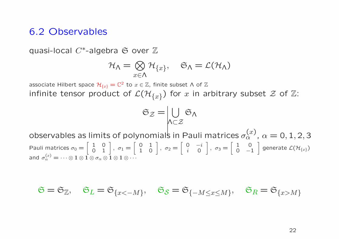
6.2 Observables

quasi-local C∗-algebra S over Z

HΛ =⊗

x∈Λ

Hx, SΛ = L(HΛ)

associate Hilbert space Hx = C2 to x ∈ Z, finite subset Λ of Z

infinite tensor product of L(Hx) for x in arbitrary subset Z of Z:

SZ =⋃

Λ⊂Z

SΛ

observables as limits of polynomials in Pauli matrices σ(x)α , α = 0,1,2,3

Pauli matrices σ0 =

[1 00 1

]

, σ1 =

[0 11 0

]

, σ2 =

[0 −ii 0

]

, σ3 =

[1 00 −1

]

generate L(Hx)

and σ(x)α = · · · ⊗ 1⊗ 1⊗ σα ⊗ 1⊗ 1⊗ · · ·

S = SZ, SL = Sx<−M, SS = S−M≤x≤M, SR = Sx>M

22

6.3 Dynamics

• local XY Hamiltonian HΛ =∑

X⊂Λ Φ(X), interaction Φ : X → SX:

Φ(X) =

−12λσ

(x)3 , X = x,

−14(1 + γ)σ

(x)1 σ

(x+1)1 + (1− γ)σ(x)

2 σ(x+1)2 , X = x, x+ 1,

0, otherwise

• thermodynamic limit of local perturbed dynamics:

τ tΛ(A) = eitHΛAe−itHΛ, τ t = limΛ→Z

τ tΛ

exists since interaction short range, two-body ⇒ defines perturbed C∗-dynamical system (S, τ)

• free dynamics from local perturbation

V = Φ(−M−1,−M)+Φ(M,M+1) ⇒ defines free C∗-dynamical system (S, τ0)

S = SL ⊗SS ⊗SR, τ t0 = τ tL ⊗ τtS ⊗ τ

tR

23

6.4 Jordan-Wigner transformation [Jordan-Wigner 28], [Araki 84]

ax := TS(x)(σ(x)1 − iσ

(x)2 )/2, S(x) =

σ(1)3 · · ·σ

(x−1)3 , x > 1

1, x = 1

σ(x)3 · · ·σ

(0)3 , x < 1

CAR A(h) with h = ℓ2(Z): ax, ay = 0 and ax, a∗y = δxy (T for two-sided chain)

• interaction becomes quadratic

φ(X) =

−12λ(2a

∗xax − 1), X = x

12a∗xax+1 + a∗x+1ax + γ(a∗xa

∗x+1 + ax+1ax), X = x, x+ 1

0, otherwise

• dynamics become Bogoliubov automorphisms

τ t(B(f)) = B(eithf), τ t0(B(f)) = B(eith0f)

[Araki 71] self-dual CAR: B(f) = a∗(f1) + a(f2) for f = (f1, f2) ∈ h⊕2

• 1-particle Hamiltonians Fourier variable ξ , V (self-dual) 2nd quantization of v

h = (cos ξ − λ)⊗ σ3 + γ sin ξ ⊗ σ2, h0 = h− v = hL ⊕ hS ⊕ hR

24

6.5 Existence and uniqueness of NESS

Theorem

Let βL, βR > 0, M ∈ N. Then:

Σ+(ω0) = ω+

Proof

• [Araki 84] βL = βR ≡ β: ω+ unique (τ, β)-KMS (RTE)

• [Kato-Birman] time dependent scattering theory for trace class type

perturbations: 1ac(h) = 1, v ∈ L0

⇒ W±(h, h0) = s−limt→±∞ eith e−ith01ac(h0) exist and are complete

completeness: ranW±(h, h0) = h(ac) (isometricity and intertwining)

γ+(B(f)) = limt→∞

τ−t0 (τ t(B(f))) = limt→∞

B(e−ith0eithf) = B(W ∗−f)

⇒ ω+ = ω0 γ+ quasifree NESS 2

25

6.6 NESS density

Theorem

ω+ has 2-point function ω+(B∗(f)B(g)) = (f, T+g) with density

T+ = (1 + e−k+)−1, k+ = (β + δ sign v−)h

v− asymptotic velocity, β = (βR + βL)/2 and δ = (βR − βL)/2

Proof

• ω+ = ω0 γ+ ⇒ T+ = W−T0W∗−

• partial wave operators wα, asymptotic projections Pαjα : ℓ2(Z)⊗ C2 → ℓ2(Zα)⊗ C2, α = L,R: canonical projections

w∗α = s−limt→−∞

eithα jα e−ith, Pα = s−limt→−∞

eith j∗αjα e−ith

[Kato-Birman], [Davies-Simon] ⇒ existence and completeness of Pα, and

W ∗− =

∑

α∈L,Rj∗αW

∗α, hαW

∗α = W ∗

α h, Pα = WαW ∗α, PL + PR = I, [Pα, h] = 0

26

• ω0 quasifree with density T0 = (1 + e−k0)−1, k0 = βL hL ⊕ 0⊕ βR hR

T+ = (1 + ek+)−1, k+ = β h+ δ (PR − PL)︸ ︷︷ ︸

= sign v−

h

v− = s-res-limt→∞ xt/t strong resolvent sense, x = −i∂ξ ⊗ 1, xt = e−ithxeith

• explicitely computable:

sign v− = sign(2λ sin ξ − (1− γ2) sin 2ξ)√

(cos ξ − λ)2 + γ2 sin2 ξ ⊗ σ0

Fourier variable ξ

2

Remarks• since k+ = βLhPL⊕βRhPR, NESS ω+ describes mixture of two independent species:”left-movers” from ranPR carry βR, ”right-movers” from ranPL carry βL

• further properties: ω+ is attractive, independent of M , translation invariant,

factor, modular, quasifree, KMS iff βL = βR, singular w.r.t. ω0

Does ω+ have nontrivial thermodynamics in the sense that its entropy

production is strictly positive?

27

6.7 Entropy production

entropy production in the open system:

Ep(ω+) = βLω+(ΦL) + βR ω+(ΦR)

ΦL = −i[H,HL], ΦR = −i[H,HR]: heat fluxes ZL, ZR → ZS

Theorem

Ep(ω+) =δ

4

∫ 2π

0

dξ

2π|κ|

sh δµ

ch 2(βµ/2) + sh 2(δµ/2)> 0 iff βL 6= βR

κ(ξ) = 2p · h = 2λ sin ξ − (1− γ2) sin 2ξ and µ(ξ) =√

(cos ξ − λ)2 + γ2 sin2 ξ

Proof explicit computation! 2

Remark

• first rigorous application of Ruelle’s scattering approach to a thermodynamically

nontrivial system

28

7. Further applications

7.1 Quasifree fermionic systems [A-Jaksic-Pautrat-Pillet 07]

NESS interaction of trace class type, no singular continuous spectrum

initial state τ t0-invariant and quasifree with density 0:

ω+(dΓ(c)) = tr(+c) with + = W−0W∗−+

∑

ε∈σpp(h)

1ε(h)01ε(h)

Landauer-Buttiker formalism derives from Ruelle’s approach:

ω+(Φq) =

∫

σac(h0)

dε

2πtr(0(ε)[q(ε)− S

∗(ε)q(ε)S(ε)])

⇒ Landauer Buttiker formula

⇒ entropy production

⇒ kinetic transport koefficients, Onsager relations

29

7.2 Weak coupling theory [A-Spohn 06]

Entropy production algebraic criterion which ensures strict positivity

in the weak coupling limit:

HS, Qj′ = C1 ⇒ Ep(ωλ+) = λ2σ(ρ0) +O(λ3) > 0

7.3 Correlations [A-Barbaroux 06], [A 07]

Spatial spin-spin correlations decay rate out of equilibrium: spectral

condition on quasifree density implies exponential decay

break translation invariance [A in progress]

von Neumann entropy density asymptotic behavior: ”left-movers”

and ”right-movers”

7.4 More...intermediate times, interacting systems, phase transitions, symme-

tries, fluctuations,...

30