Embed Size (px)
Citation preview
A short introduction to the computation of standard errors for AF measures
A short introduction to the computation ofstandard errors for AF measures
Gaston Yalonetzky
Oxford Poverty and Human Development Initiative, University of Oxford
OPHI-HDCA Summer School, Delft, 24 August - 3 September2011.
We are grateful to the World Bank, two anonymous donors andOPHI for financial support

A short introduction to the computation of standard errors for AF measures
Table of contents
Introduction
Computing the standard errors of averages in simple surveys
Asymptotic standard errors for ratios
Asymptotic standard errors for percentage changesPercentage changes in cross sectionsPercentage changes in panel data
Computation of standard errors with more complex surveys
Concluding remarks
A short introduction to the computation of standard errors for AF measures
Introduction
Introduction: Standard errors for the AF measures
I The computation of standard errors is fundamental for theperformance of statistical inference and the production ofconfidence intervals.
I In classical statistics there are two ways of producing standarderrors:
1. Applying the formulas of analytically derived standard errors.Sometimes these can only be asymptotic approximations (wewill see a couple of these).
2. With resampling methods (not covered in this lecture, butsome references given at the end).

A short introduction to the computation of standard errors for AF measures
Introduction
Introduction: Standard errors for the AF measures
In this lecture we will:
I Quickly review how we compute a standard error for H in thecase of a simple random sample.
I Study how we can derive asymptotic standard errors using Aas an example.
I Derive asymptotic standard errors for ∆% for cross-sectionsand panel datasets.
I Briefly discuss computation of standard errors when we havemore complex surveys.
A short introduction to the computation of standard errors for AF measures
Computing the standard errors of averages in simple surveys
Computing the standard error of H
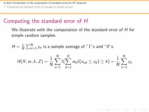
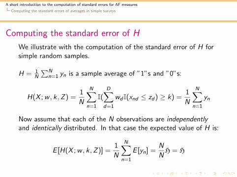
We illustrate with the computation of the standard error of H forsimple random samples.
H = 1N
∑Nn=1 yn is a sample average of ”1”s and ”0”s:
H(X ;w , k ,Z ) =1
N
N∑n=1
I(D∑
d=1
wdI(xnd ≤ zd) ≥ k) =1
N
N∑n=1
yn
Now assume that each of the N observations are independentlyand identically distributed. In that case the expected value of H is:
E [H(X ;w , k ,Z )] =1
N
N∑n=1
E [yn] =N
NH = H
A short introduction to the computation of standard errors for AF measures
Computing the standard errors of averages in simple surveys
Computing the standard error of H
We illustrate with the computation of the standard error of H forsimple random samples.
H = 1N
∑Nn=1 yn is a sample average of ”1”s and ”0”s:
H(X ;w , k ,Z ) =1
N
N∑n=1
I(D∑
d=1
wdI(xnd ≤ zd) ≥ k) =1
N
N∑n=1
yn
Now assume that each of the N observations are independentlyand identically distributed. In that case the expected value of H is:
E [H(X ;w , k ,Z )] =1
N
N∑n=1
E [yn] =N
NH = H

A short introduction to the computation of standard errors for AF measures
Computing the standard errors of averages in simple surveys
Computing the standard error of H
We illustrate with the computation of the standard error of H forsimple random samples.
H = 1N
∑Nn=1 yn is a sample average of ”1”s and ”0”s:
H(X ;w , k ,Z ) =1
N
N∑n=1
I(D∑
d=1
wdI(xnd ≤ zd) ≥ k) =1
N
N∑n=1
yn
Now assume that each of the N observations are independentlyand identically distributed.
In that case the expected value of H is:
E [H(X ;w , k ,Z )] =1
N
N∑n=1
E [yn] =N
NH = H
A short introduction to the computation of standard errors for AF measures
Computing the standard errors of averages in simple surveys
Computing the standard error of H
We illustrate with the computation of the standard error of H forsimple random samples.
H = 1N
∑Nn=1 yn is a sample average of ”1”s and ”0”s:
H(X ;w , k ,Z ) =1
N
N∑n=1
I(D∑
d=1
wdI(xnd ≤ zd) ≥ k) =1
N
N∑n=1
yn
Now assume that each of the N observations are independentlyand identically distributed. In that case the expected value of H is:
E [H(X ;w , k ,Z )] =1
N
N∑n=1
E [yn] =N
NH = H

A short introduction to the computation of standard errors for AF measures
Computing the standard errors of averages in simple surveys
Computing the standard error of H
We illustrate with the computation of the standard error of H forsimple random samples.
H = 1N
∑Nn=1 yn is a sample average of ”1”s and ”0”s:
H(X ;w , k ,Z ) =1
N
N∑n=1
I(D∑
d=1
wdI(xnd ≤ zd) ≥ k) =1
N
N∑n=1
yn
Now assume that each of the N observations are independentlyand identically distributed. In that case the expected value of H is:
E [H(X ;w , k ,Z )] =1
N
N∑n=1
E [yn] =N
NH = H

A short introduction to the computation of standard errors for AF measures
Computing the standard errors of averages in simple surveys
Computing the standard error of H
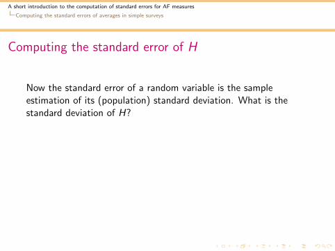
Now the standard error of a random variable is the sampleestimation of its (population) standard deviation.
What is thestandard deviation of H? We need its variance first. Let’s look atthe population variance:
E [H − H]2 =1
N2Nσ2
I =1
Nσ2I
σ2I = E [yn − H]2 = E [y2
n ]− H2
A short introduction to the computation of standard errors for AF measures
Computing the standard errors of averages in simple surveys
Computing the standard error of H
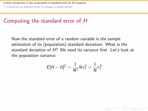
Now the standard error of a random variable is the sampleestimation of its (population) standard deviation. What is thestandard deviation of H?
We need its variance first. Let’s look atthe population variance:
E [H − H]2 =1
N2Nσ2
I =1
Nσ2I
σ2I = E [yn − H]2 = E [y2
n ]− H2

A short introduction to the computation of standard errors for AF measures
Computing the standard errors of averages in simple surveys
Computing the standard error of H
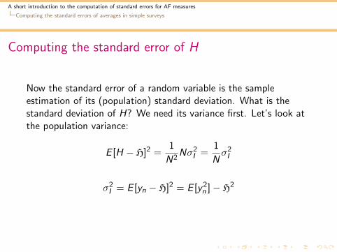
Now the standard error of a random variable is the sampleestimation of its (population) standard deviation. What is thestandard deviation of H? We need its variance first. Let’s look atthe population variance:
E [H − H]2 =1
N2Nσ2
I =1
Nσ2I
σ2I = E [yn − H]2 = E [y2
n ]− H2
A short introduction to the computation of standard errors for AF measures
Computing the standard errors of averages in simple surveys
Computing the standard error of H
Now the standard error of a random variable is the sampleestimation of its (population) standard deviation. What is thestandard deviation of H? We need its variance first. Let’s look atthe population variance:
E [H − H]2 =1
N2Nσ2
I =1
Nσ2I
σ2I = E [yn − H]2 = E [y2
n ]− H2

A short introduction to the computation of standard errors for AF measures
Computing the standard errors of averages in simple surveys
Computing the standard error of H
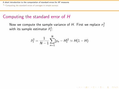
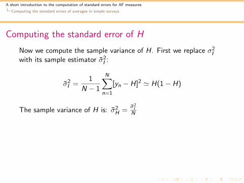
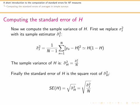
Now we compute the sample variance of H.
First we replace σ2I
with its sample estimator σ̄2I :
σ̄2I =
1
N − 1
N∑n=1
[yn − H]2 ' H(1− H)
The sample variance of H is: σ̄2H =
σ̄2IN
Finally the standard error of H is the square root of σ̄2H :
SE (H) =√σ̄2H =
√σ̄2I
N
A short introduction to the computation of standard errors for AF measures
Computing the standard errors of averages in simple surveys
Computing the standard error of H
Now we compute the sample variance of H. First we replace σ2I
with its sample estimator σ̄2I :
σ̄2I =
1
N − 1
N∑n=1
[yn − H]2 ' H(1− H)
The sample variance of H is: σ̄2H =
σ̄2IN
Finally the standard error of H is the square root of σ̄2H :
SE (H) =√σ̄2H =
√σ̄2I
N

A short introduction to the computation of standard errors for AF measures
Asymptotic standard errors for ratios
Asymptotic standard errors for ratios like A
For other averages, like Mα, the procedure to compute standarderrors using simple surveys is the same as outlined before for H.
In STATA this is done easily by generating the respective variableyn and then using the command ”summarize”.
However, this procedure cannot be implemented when we haveratios of random variables, (as opposed to averages based onsums). In the AF family we have ratios like A. For these variableswe need to compute asymptotic standard errors.

A short introduction to the computation of standard errors for AF measures
Asymptotic standard errors for ratios
Asymptotic standard errors for ratios like A
For other averages, like Mα, the procedure to compute standarderrors using simple surveys is the same as outlined before for H.
In STATA this is done easily by generating the respective variableyn and then using the command ”summarize”.
However, this procedure cannot be implemented when we haveratios of random variables, (as opposed to averages based onsums).
In the AF family we have ratios like A. For these variableswe need to compute asymptotic standard errors.

A short introduction to the computation of standard errors for AF measures
Asymptotic standard errors for ratios
Asymptotic standard errors for ratios like A
For other averages, like Mα, the procedure to compute standarderrors using simple surveys is the same as outlined before for H.
In STATA this is done easily by generating the respective variableyn and then using the command ”summarize”.
However, this procedure cannot be implemented when we haveratios of random variables, (as opposed to averages based onsums). In the AF family we have ratios like A. For these variableswe need to compute asymptotic standard errors.

A short introduction to the computation of standard errors for AF measures
Asymptotic standard errors for ratios
Asymptotic standard errors for ratios like A
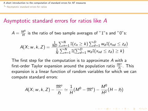
A = M0
H is the ratio of two sample averages of ”1”s and ”0”s:
A(X ;w , k ,Z ) =1
ND
∑Nn=1 I(cn ≥ k)
∑Dd=1 wdI(xnd ≤ zd)
1N
∑Nn=1 I(
∑Dd=1 wdI(xnd ≤ zd) ≥ k)
The first step for the computation is to approximate A with afirst-order Taylor expansion around the population ratio M0
H . Thisexpansion is a linear function of random variables for which we cancompute standard errors:
A(X ;w , k ,Z )− M0
H' 1
H(M0 −M0)− M0
H2(H − H)

A short introduction to the computation of standard errors for AF measures
Asymptotic standard errors for ratios
Asymptotic standard errors for ratios like A
A = M0
H is the ratio of two sample averages of ”1”s and ”0”s:
A(X ;w , k ,Z ) =1
ND
∑Nn=1 I(cn ≥ k)
∑Dd=1 wdI(xnd ≤ zd)
1N
∑Nn=1 I(
∑Dd=1 wdI(xnd ≤ zd) ≥ k)
The first step for the computation is to approximate A with afirst-order Taylor expansion around the population ratio M0
H .
Thisexpansion is a linear function of random variables for which we cancompute standard errors:
A(X ;w , k ,Z )− M0
H' 1
H(M0 −M0)− M0
H2(H − H)
A short introduction to the computation of standard errors for AF measures
Asymptotic standard errors for ratios
Asymptotic standard errors for ratios like A
A = M0
H is the ratio of two sample averages of ”1”s and ”0”s:
A(X ;w , k ,Z ) =1
ND
∑Nn=1 I(cn ≥ k)
∑Dd=1 wdI(xnd ≤ zd)
1N
∑Nn=1 I(
∑Dd=1 wdI(xnd ≤ zd) ≥ k)
The first step for the computation is to approximate A with afirst-order Taylor expansion around the population ratio M0
H . Thisexpansion is a linear function of random variables for which we cancompute standard errors:
A(X ;w , k ,Z )− M0
H' 1
H(M0 −M0)− M0
H2(H − H)
A short introduction to the computation of standard errors for AF measures
Asymptotic standard errors for ratios
Asymptotic standard errors for ratios like A
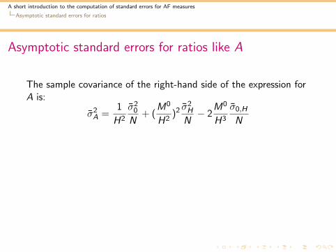
The sample covariance of the right-hand side of the expression forA is:
σ̄2A =
1
H2
σ̄20
N+ (
M0
H2)2 σ̄
2H
N− 2
M0
H3
σ̄0,H
N
Where:
σ̄20 =
1
N − 1
N∑n=1
[I(cn ≥ k)cn −M0]2
σ̄0,H ' M0[1− H]
Finally SE (A) =√σ̄2A
A short introduction to the computation of standard errors for AF measures
Asymptotic standard errors for ratios
Asymptotic standard errors for ratios like A
The sample covariance of the right-hand side of the expression forA is:
σ̄2A =
1
H2
σ̄20
N+ (
M0
H2)2 σ̄
2H
N− 2
M0
H3
σ̄0,H
N
Where:
σ̄20 =
1
N − 1
N∑n=1
[I(cn ≥ k)cn −M0]2
σ̄0,H ' M0[1− H]
Finally SE (A) =√σ̄2A
A short introduction to the computation of standard errors for AF measures
Asymptotic standard errors for percentage changes
Asymptotic standard errors for ∆%
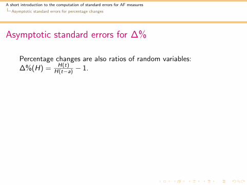
Percentage changes are also ratios of random variables:∆%(H) = H(t)
H(t−a) − 1.
Hence a similar approach to the one used forA is required:
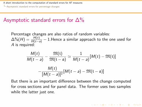
M(t)
M(t − a)− M(t)
M(t− a)' 1
M(t − a)[M(t)−M(t)]
− M(t)
[M(t − a)]2[M(t − a)−M(t− a)]
But there is an important difference between the change computedfor cross sections and for panel data. The former uses two sampleswhile the latter just one.

A short introduction to the computation of standard errors for AF measures
Asymptotic standard errors for percentage changes
Asymptotic standard errors for ∆%
Percentage changes are also ratios of random variables:∆%(H) = H(t)
H(t−a) − 1.Hence a similar approach to the one used forA is required:
M(t)
M(t − a)− M(t)
M(t− a)' 1
M(t − a)[M(t)−M(t)]
− M(t)
[M(t − a)]2[M(t − a)−M(t− a)]
But there is an important difference between the change computedfor cross sections and for panel data. The former uses two sampleswhile the latter just one.

A short introduction to the computation of standard errors for AF measures
Asymptotic standard errors for percentage changes
Percentage changes in cross sections
Asymptotic standard errors for ∆% in cross sections
The asymptotic variance of Mα is:
σ̄2∆%Mα =
1
[M(t − a)]2
σ̄2α(t)
N(t)+ [
Mα(t)
[Mα(t − a)]2]2σ̄2α(t−a)
N(t − a)
Then the standard error is:
SE (∆%Mα) =√σ̄2
∆%Mα

A short introduction to the computation of standard errors for AF measures
Asymptotic standard errors for percentage changes
Percentage changes in panel data
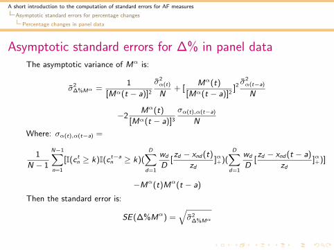
Asymptotic standard errors for ∆% in panel dataThe asymptotic variance of Mα is:
σ̄2∆%Mα =
1
[Mα(t − a)]2
σ̄2α(t)
N+ [
Mα(t)
[Mα(t − a)]2]2 σ̄
2α(t−a)
N
−2Mα(t)
[Mα(t − a)]3
σα(t),α(t−a)
N
Where: σα(t),α(t−a) =
1
N − 1
N−1∑n=1
[I(c tn ≥ k)I(c t−an ≥ k)(
D∑d=1
wd
D[zd − xnd(t)
zd]α+)(
D∑d=1
wd
D[zd − xnd(t − a)
zd]α+)]
−Mα(t)Mα(t − a)
Then the standard error is:
SE(∆%Mα) =√
σ̄2∆%Mα

A short introduction to the computation of standard errors for AF measures
Asymptotic standard errors for percentage changes
Percentage changes in panel data
Asymptotic standard errors for ∆% in panel dataThe asymptotic variance of Mα is:
σ̄2∆%Mα =
1
[Mα(t − a)]2
σ̄2α(t)
N+ [
Mα(t)
[Mα(t − a)]2]2 σ̄
2α(t−a)
N
−2Mα(t)
[Mα(t − a)]3
σα(t),α(t−a)
N
Where: σα(t),α(t−a) =
1
N − 1
N−1∑n=1
[I(c tn ≥ k)I(c t−an ≥ k)(
D∑d=1
wd
D[zd − xnd(t)
zd]α+)(
D∑d=1
wd
D[zd − xnd(t − a)
zd]α+)]
−Mα(t)Mα(t − a)
Then the standard error is:
SE(∆%Mα) =√
σ̄2∆%Mα
A short introduction to the computation of standard errors for AF measures
Computation of standard errors with more complex surveys
Standard errors with complex surveysDifferent types of surveys are available.
For instance, some of the countrysurveys included in the EU-SILC are simple and random; however mosthousehold surveys tend to be more complex, especially they tend to betwo-stage, stratified.
When computing standard errors the survey features need to be taken intoaccount, in particular:
I Strata
I Clusters
I Sampling weights
The formulas can be adapted easily (although a bit tediously) following
Deaton’s book ”The analysis of household surveys” (1997)
In STATA this is done very easily by first indicating the variables that contain
the survey information (with svyset) and then using ”svy: sum” to produce the
required statistics.

A short introduction to the computation of standard errors for AF measures
Computation of standard errors with more complex surveys
Standard errors with complex surveysDifferent types of surveys are available. For instance, some of the countrysurveys included in the EU-SILC are simple and random; however mosthousehold surveys tend to be more complex, especially they tend to betwo-stage, stratified.
When computing standard errors the survey features need to be taken intoaccount, in particular:
I Strata
I Clusters
I Sampling weights
The formulas can be adapted easily (although a bit tediously) following
Deaton’s book ”The analysis of household surveys” (1997)
In STATA this is done very easily by first indicating the variables that contain
the survey information (with svyset) and then using ”svy: sum” to produce the
required statistics.

A short introduction to the computation of standard errors for AF measures
Computation of standard errors with more complex surveys
Example of how STATA handles complex surveysImagine we want to compute the standard error of H and thevariable identifying households as poor is called ”mdpoor”.
In the quite typical case of a stratified two-stage survey, first onetells STATA what are the variables that indicate clusters, strataand weights: pause
svyset: namecluster [pweight=nameweight], strata(namestrata) ||householdid
Then one can estimate the standard error of H using the commandsvy: mean applied to ”mdpoor”:
svy: mean poor
A short introduction to the computation of standard errors for AF measures
Computation of standard errors with more complex surveys
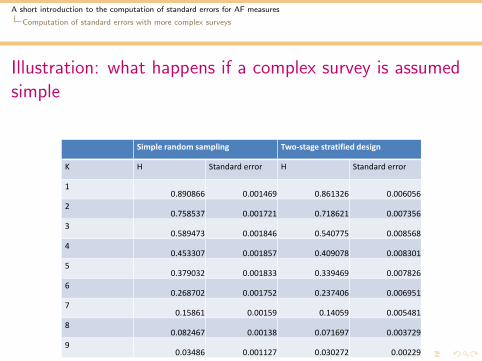
Illustration: what happens if a complex survey is assumedsimple
������������ ����� �� �� ��� ����������� ��
� � �������� ��� � ������������
� ��� ��� � ���� ������� � � ��
� ������� � ���� ������� � ����
� ������� � ���� ��� ��� � ����
� ����� � � ���� �� � �� � �� �
� ���� �� � ���� ������� � ����
� ����� � � ���� ����� � � ����
� ������ � ��� ��� �� � ����
� � ����� � ��� � ����� � ����
� � ���� � ���� � � ��� � ���

A short introduction to the computation of standard errors for AF measures
Concluding remarks
Concluding remarks
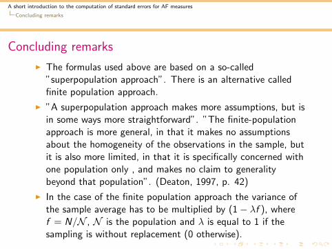
I The formulas used above are based on a so-called”superpopulation approach”.
There is an alternative calledfinite population approach.
I ”A superpopulation approach makes more assumptions, but isin some ways more straightforward”. ”The finite-populationapproach is more general, in that it makes no assumptionsabout the homogeneity of the observations in the sample, butit is also more limited, in that it is specifically concerned withone population only , and makes no claim to generalitybeyond that population”. (Deaton, 1997, p. 42)
I In the case of the finite population approach the variance ofthe sample average has to be multiplied by (1− λf ), wheref = N/N , N is the population and λ is equal to 1 if thesampling is without replacement (0 otherwise).
A short introduction to the computation of standard errors for AF measures
Concluding remarks
Concluding remarks
I The formulas used above are based on a so-called”superpopulation approach”. There is an alternative calledfinite population approach.
I ”A superpopulation approach makes more assumptions, but isin some ways more straightforward”.
”The finite-populationapproach is more general, in that it makes no assumptionsabout the homogeneity of the observations in the sample, butit is also more limited, in that it is specifically concerned withone population only , and makes no claim to generalitybeyond that population”. (Deaton, 1997, p. 42)
I In the case of the finite population approach the variance ofthe sample average has to be multiplied by (1− λf ), wheref = N/N , N is the population and λ is equal to 1 if thesampling is without replacement (0 otherwise).
A short introduction to the computation of standard errors for AF measures
Concluding remarks
Concluding remarks
I The formulas used above are based on a so-called”superpopulation approach”. There is an alternative calledfinite population approach.
I ”A superpopulation approach makes more assumptions, but isin some ways more straightforward”. ”The finite-populationapproach is more general, in that it makes no assumptionsabout the homogeneity of the observations in the sample, butit is also more limited, in that it is specifically concerned withone population only , and makes no claim to generalitybeyond that population”. (Deaton, 1997, p. 42)
I In the case of the finite population approach the variance ofthe sample average has to be multiplied by (1− λf ), wheref = N/N , N is the population and λ is equal to 1 if thesampling is without replacement (0 otherwise).
A short introduction to the computation of standard errors for AF measures
Concluding remarks
Concluding remarks
I The formulas used above are based on a so-called”superpopulation approach”. There is an alternative calledfinite population approach.
I ”A superpopulation approach makes more assumptions, but isin some ways more straightforward”. ”The finite-populationapproach is more general, in that it makes no assumptionsabout the homogeneity of the observations in the sample, butit is also more limited, in that it is specifically concerned withone population only , and makes no claim to generalitybeyond that population”. (Deaton, 1997, p. 42)
I In the case of the finite population approach the variance ofthe sample average has to be multiplied by (1− λf ), wheref = N/N , N is the population and λ is equal to 1 if thesampling is without replacement (0 otherwise).

A short introduction to the computation of standard errors for AF measures
Concluding remarks
Concluding remarks
I In practice the differences in estimates using the twoapproaches are likely to be minimal.
I It is good practice to check for the formulas of differentsurvey designs in survey design textbooks. Household surveyscome with manuals that (ideally) explain what survey designwas implemented.
I An alternative to analytically derived standard errors isprovided by resampling methods (e.g. bootstraps, jackknifes).There are several of these and they can be quite useful whenderivation becomes cumbersome. For some discussion andexamples see Kolenikov (”Resampling inference with complexsurvey data”) and Rao (”Bootstrap methods for analyzingcomplex sample survey data”).

A short introduction to the computation of standard errors for AF measures
Concluding remarks
Concluding remarks
I In practice the differences in estimates using the twoapproaches are likely to be minimal.
I It is good practice to check for the formulas of differentsurvey designs in survey design textbooks.
Household surveyscome with manuals that (ideally) explain what survey designwas implemented.
I An alternative to analytically derived standard errors isprovided by resampling methods (e.g. bootstraps, jackknifes).There are several of these and they can be quite useful whenderivation becomes cumbersome. For some discussion andexamples see Kolenikov (”Resampling inference with complexsurvey data”) and Rao (”Bootstrap methods for analyzingcomplex sample survey data”).
A short introduction to the computation of standard errors for AF measures
Concluding remarks
Concluding remarks
I In practice the differences in estimates using the twoapproaches are likely to be minimal.
I It is good practice to check for the formulas of differentsurvey designs in survey design textbooks. Household surveyscome with manuals that (ideally) explain what survey designwas implemented.
I An alternative to analytically derived standard errors isprovided by resampling methods (e.g. bootstraps, jackknifes).There are several of these and they can be quite useful whenderivation becomes cumbersome. For some discussion andexamples see Kolenikov (”Resampling inference with complexsurvey data”) and Rao (”Bootstrap methods for analyzingcomplex sample survey data”).

A short introduction to the computation of standard errors for AF measures
Concluding remarks
Concluding remarks
I In practice the differences in estimates using the twoapproaches are likely to be minimal.
I It is good practice to check for the formulas of differentsurvey designs in survey design textbooks. Household surveyscome with manuals that (ideally) explain what survey designwas implemented.
I An alternative to analytically derived standard errors isprovided by resampling methods (e.g. bootstraps, jackknifes).There are several of these and they can be quite useful whenderivation becomes cumbersome.
For some discussion andexamples see Kolenikov (”Resampling inference with complexsurvey data”) and Rao (”Bootstrap methods for analyzingcomplex sample survey data”).
A short introduction to the computation of standard errors for AF measures
Concluding remarks
Concluding remarks
I In practice the differences in estimates using the twoapproaches are likely to be minimal.
I It is good practice to check for the formulas of differentsurvey designs in survey design textbooks. Household surveyscome with manuals that (ideally) explain what survey designwas implemented.
I An alternative to analytically derived standard errors isprovided by resampling methods (e.g. bootstraps, jackknifes).There are several of these and they can be quite useful whenderivation becomes cumbersome. For some discussion andexamples see Kolenikov (”Resampling inference with complexsurvey data”) and Rao (”Bootstrap methods for analyzingcomplex sample survey data”).