A sensitivity theory for the equilibrium boundary layer over land

Timothy W. Cronin1

Received 11 April 2013; revised 24 July 2013; accepted 16 September 2013; published 4 November 2013.

[1] Due to the intrinsic complexities associated with modeling land-atmosphere inter-actions, global models typically use elaborate land surface and boundary layer physicsparameterizations. Unfortunately, it is difficult to use elaborate models, by them-selves, to develop a deeper understanding of how land surface parameters affect thecoupled land-atmosphere system. At the same time, it is also increasingly important togain a deeper understanding of the role of changes in land cover, land use, and ecosys-tem function as forcings and feedbacks in past and future climate change. To improvethe foundation of our understanding, we outline a framework for boundary layer cli-mate sensitivity based on surface energy balance; just as global climate sensitivity isbased on top-of-atmosphere energy balance. We develop an analytic theory for theboundary layer climate sensitivity of an idealized model of a diurnally averaged well-mixed boundary layer over land. This analytic sensitivity theory identifies changes inthe properties of the land surface—including moisture availability, albedo, and aero-dynamic roughness—as forcings, and identifies strong negative feedbacks associatedwith the surface fluxes of latent and sensible heat. We show that our theory canexplain nearly all of the sensitivity of the Betts (2000) full system of equations. Favor-able comparison of the theory and the simulation results from a two-column radiativeconvective model suggests that the theory may be broadly useful for unifying ourunderstanding of how changes in land use or ecosystem function may affect climatechange.

Citation: Cronin, T. W. (2013), A sensitivity theory for the equilibrium boundary layer over land, J. Adv. Model. Earth Syst., 5, 764–

784, doi:10.1002/jame.20048.

1. Introduction

[2] Global-mean surface air temperature is controlledprimarily by planetary energy balance, in which green-house gas concentrations and the planetary albedo playa dominant role. Simple models of the sensitivity ofplanetary energy balance to greenhouse gas concentra-tions form the foundation of our understanding of howwell-mixed greenhouse gases, such as anthropogenicCO2, affect global climate. Land surface properties,such as moisture availability and roughness, play less ofa role in determining the global-mean surface tempera-ture, but they can strongly affect local surface tempera-tures, with disproportionately large impacts on society.The potential importance of climate change forced byland surface changes ought to be a concern in any com-prehensive study of climate change, because the human

footprint on the land surface is large, and rapidlychanging.

[3] In order to both simulate and understand impor-tant problems related to the climate system, Held [2005]argues for the importance of model hierarchies, withmodels that span a range of complexity levels. Since theearly and influential studies of Charney [1975] and Shu-kla and Mintz [1982], much valuable work has beendone to simulate the impacts of the land surface on theclimate (and vice versa) with highly complex general cir-culation models (GCMs). Toward the simpler end ofthe complexity spectrum, idealized models of thecoupled surface-boundary layer system have done agreat deal to advance our understanding of land-atmosphere interactions [e.g., McNaughton and Spriggs,1986; Jacobs and De Bruin, 1992; Brubaker and Ente-khabi, 1995; Kim and Entekhabi, 1998]. One of the cen-tral motivations of this work is our belief that theexisting model hierarchies in the field of land-atmosphere interactions do not extend down to modelsthat are sufficiently simple so as to be analytically trac-table, and that the lack of analytic models and frame-works impedes the understanding and synthesis ofresults from more complex models. Despite the largebody of work with both simple and complex models,there remains no widely accepted corollary to climate

1Program in Atmospheres, Oceans, and Climate, MassachusettsInstitute of Technology, Cambridge, MA, 02139, USA.

Corresponding author: T. W. Cronin, Program in Atmospheres,Oceans, and Climate, Massachusetts Institute of Technology, 77 Mas-sachusetts Ave., Cambridge, MA 02139, USA. (twcronin@mit.edu)

©2013. American Geophysical Union. All Rights Reserved.1942-2466/13/10.1002/jame.20048

764

JOURNAL OF ADVANCES IN MODELING EARTH SYSTEMS, VOL. 5, 764–784, doi:10.1002/jame.20048, 2013

sensitivity when it comes to understanding the impactof land surface properties on changes in near-surfacetemperatures.

[4] In this study, we attempt to define such a corol-lary to climate sensitivity, by introducing the frame-work of boundary layer climate sensitivity. We suggestthat daily-average regional temperature response due tochanges in surface moisture availability, albedo, androughness can be understood within a context of forc-ings and feedbacks, similar to the case of global climateresponse to a radiative perturbation, but based on sur-face energy balance, rather than top-of-atmosphereenergy balance. Many of the aspects of our work arenot new; numerous other studies have used the lan-guage of sensitivity theory to describe feedbacks (andoccasionally forcings) in the coupled land-atmospheresystem. Because of the importance of the diurnal cyclefor land-atmosphere exchanges of water, energy, andmomentum, such studies have often focused on the roleof feedbacks in the evolution of temperature and evapo-ration over only a single day [Jacobs and De Bruin,1992; van Heerwaarden et al., 2009, 2010]. In such work,initial conditions are often of major importance, andmodel results are compared to observations of weather,rather than climate.

[5] Our work focuses on longer time scales, emphasiz-ing the importance of land surface properties in deter-mining daily-average surface and boundary layertemperatures. Because of the relative unimportance ofthe diurnal cycle for ocean-atmosphere coupling, theequilibrium climate of the surface-boundary layer sys-tem over the ocean is more easily defined, observed,and modeled [Betts and Ridgway, 1988, 1989]. Theproblem of the daily-average state of the coupledsurface-boundary layer system over land was tackledlater, first by models with fixed boundary layer depth[Brubaker and Entekhabi, 1995; Entekhabi and Bru-baker, 1995; Brubaker and Entekhabi, 1996], then bymodels with variable boundary layer depth [Kim andEntekhabi, 1998; Betts, 2000]. The elegant studies ofEntekhabi and Brubaker [1995] and Brubaker and Ente-khabi [1996] used an idealized model to explore thefeedbacks that serve to amplify or dampen forced soilmoisture and temperature variability over time scales ofdays to months. However, the temperature variabilityin their work was forced by wind speed, rather than anychanges in land surface properties, and their assump-tion of constant boundary layer height cuts the impor-tant connection between warming and boundary layerdeepening, as well as any control on boundary layertemperatures exerted by the free troposphere. Our workwill build off the diurnally averaged mixed layer-surfacemodel of Betts [2000], which has a very simple treat-ment of radiation and surface turbulent exchange, butrelaxes the constant-height assumption of Brubaker andEntekhabi [1995] and the constant specific humidityassumption of Kim and Entekhabi [1998].

[6] Based on the model of Betts [2000], we derive ana-lytic expressions for the response of surface temperatureand boundary layer potential temperature to forcing byperturbations in surface moisture availability, albedo,

and roughness. As in the studies of Brubaker and Ente-khabi [1996] and Kim and Entekhabi [1998], our theoryassociates the strongest negative feedback with the de-pendence of the surface latent heat flux on saturationvapor pressure. We compare the results from our analytictheory to the full model of Betts [2000] and show that ourtheory can explain nearly all of the sensitivity of the Betts[2000] full system of equations. As in the case of the non-linear (approximately logarithmic) radiative forcing byCO2, we find that allowance for nonlinear forcing func-tions is important, especially for large changes in surfacemoisture availability and roughness. We find that thetheory agrees well with simulation results from a morecomplex two-column radiative-convective model, and wediscuss limitations of the theory. We conclude by discus-sing how our theory may allow for a more unified under-standing of the boundary layer climate response todisparate problems such as urbanization, deforestation,drought, and CO2-induced stomatal closure.

2. Theory

2.1. Framework for Boundary Layer Sensitivity

[7] Top-of-atmosphere radiative energy balanceserves as the guiding principle in the theory of globalclimate sensitivity:

RS2RL50; ð1Þ

where RS is the top-of atmosphere net downward short-wave radiation absorbed by the Earth, and RL is thetop-of-atmosphere net longwave radiation emitted bythe Earth. To understand how an arbitrary forcing pa-rameter, A (e.g., CO2), affects the climate near a knownreference state, we take the total derivative of top-of-atmosphere energy balance with respect to A:

dRS

dA2

dRL

dA50: ð2Þ

[8] We expand the total derivatives into forcings (e.g.,@RL=@A), plus products of feedbacks and responses(e.g., @RL=@Tð Þ dT=dAð Þ, where T represents globaltemperature), and then solve for the response as thesum of forcings divided by the sum of feedbacks. Such adecomposition of the climate response to increasingconcentrations of well-mixed greenhouse gases hashelped us to standardize model simulations, focus studyon key mechanisms that mediate the strength of the cli-mate response, and identify ways in which modelsresemble or differ from one another.

[9] We propose a similar framework for boundary-layer climate sensitivity, with a guiding principle of surfaceenergy balance. Assuming a long-term equilibrium withno subsurface heat flux, surface energy balance is given by

QS2QL2H2E50; ð3Þ

where QS is the net shortwave radiation at the surface(positive downward), QL is the net longwave radiation

CRONIN: BOUNDARY LAYER SENSITIVITY THEORY

765

at the surface (positive upward), E is the latent heatflux, and H is the sensible heat flux (both defined to bepositive upward). To apply a sensitivity framework tothe problem, we begin by taking the total derivative of(3) with respect to the arbitrary variable A, near a well-defined reference state of the surface-boundary layersystem, where surface energy balance holds:

dQS

dA2

dQL

dA2

dH

dA2

dE

dA50: ð4Þ

[10] Expansion of each of these total derivatives bythe chain rule is algebraically complicated and requiresus to define which controlling variables to include inour expansion of (4). We suggest that the set of control-ling variables should include at least the ground temper-ature, TS, the near-surface potential temperature of theboundary layer, hM, and the near-surface specific hu-midity of the boundary layer, qM (these are also three ofthe prognostic variables in the idealized model of Bru-baker and Entekhabi [1995]). Variables related to cloudi-ness, especially low-level cloud fraction and water path,may also be quite important, but we will not considerthem explicitly in our example case below.

[11] Once such a set of controlling variables is defined,we can define a boundary layer climate sensitivity by:

[12] 1. Eliminating all but one controlling variable byidentifying relationships among them (e.g., by linearlyrelating changes in TS and qM to changes in hM)

[13] 2. Evaluating, theoretically or empirically, thepartial derivatives of the surface fluxes with respect tothe controlling variables (terms such as @E=@TS)

[14] 3. Algebraically rearranging to solve for howchanges in a controlling variable are affected bychanges in a forcing variable, dA

[15] The framework proposed here may seem abstractand somewhat open ended, but this is intended for gen-erality. In order to apply this framework to a GCM,one would likely have to conduct a suite of perturbationexperiments. The relationships among controlling vari-ables, as well as the partial derivatives of surface fluxeswith respect to controlling variables, could be evaluatedby multiple linear regression.

[16] In order to provide a more concrete example ofthe proposed framework, the remainder of the theorysection will be devoted to deriving the boundary layersensitivity of a highly idealized model of the equilibriumboundary layer, as presented by Betts [2000]. Withappropriate simplifications and assumptions, it willturn out that we can actually arrive at an analyticexpression for the sensitivity of the equilibrium bound-ary layer to forcing by changes in various surface pa-rameters. For the convenience of a reader who isinterested in our ideas but not our detailed derivation,we include the key equations from the analytic sensitiv-ity theory (sections 2.2–2.7) in Tables 1 and 2.

2.2. Equilibrium Boundary Layer Model of Betts [2000]

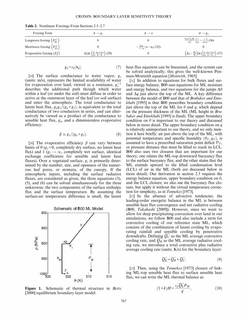
[17] Following the work by Betts [2000] (hereafterB00), we seek to understand the problem of the surface-atmosphere interaction by considering equations for thetime-mean surface temperature TS, and the time-meanboundary layer potential temperature and specific hu-midity, hM and qM, in a well-mixed boundary layer(ML) (see Figure 1 for a schematic of the thermal struc-ture). Here, we review some of the key model assump-tions from B00.

[18] Following commonly used conventions [e.g.,Allen et al., 1998; Jones, 1992], B00 defines bulk formu-lae for the latent and sensible heat fluxes E and H asfollows:

E5qLv

gagv

ga1gv

q� TSð Þ2qMð Þ; ð5Þ

H5qcpga TS2hMð Þ; ð6Þ

where q is the density of air, Lv is the latent heat of va-porization of water, cp is the specific heat capacity ofair, q� TSð Þ is the saturation mixing ratio of water vaporat surface temperature (for simplicity, we assume thatthe surface pressure equals the reference pressure in thedefinition of h). The surface conductance to sensibleheat flux, ga (units: m/s), can be written as the productof a nondimensional enthalpy flux coefficient, ck, and asurface wind speed, jvsj:

Table 1. Key Equations From the Analytic Sensitivity Theory of Sections 2.2–2.7

Description Expression Equation Number

General sensitivity equation dhM52FA

QL1F A

E2FA

QS

kH 1kE 1kQL2kQS

(22)

Sensible heat flux feedback kH 5qcpgac (25)

Evaporative feedback kE5qLvgagv

ga1gv

@q�

@T

���TS0

11c2n @q�

@T

� �21� �

(26)

Longwave feedback kQL54rBT3

S0c (27)

Relationship between dTS and dhM dTS52 1qcpga

@H@A

dA1 11cð ÞdhM (16)

Relationship between dqM and dhM dqM5ndhM (20)

Parameter relating dTS to dhM c5 QR

qgagC 11kð Þ (17)

Parameter relating dqM to dhM n5@q�

@T

���Tb

ps

pb

� �Rcp

12 RhM

cppbC

� �1

qM

pbC

� �(21)

CRONIN: BOUNDARY LAYER SENSITIVITY THEORY

766

ga5ckjvsj: ð7Þ

[19] The surface conductance to water vapor, gv

(units: m/s), represents the limited availability of waterfor evaporation over land; viewed as a resistance, g21

vdescribes the additional path though which waterwithin a leaf (or under the soil) must diffuse in order toarrive at the outermost layer of the leaf (or soil surface)and enter the atmosphere. The total conductance tolatent heat flux, gagv= ga1gvð Þ, is equivalent to the totalconductance of two conductors in series, and can alter-natively be viewed as a product of the conductance tosensible heat flux, ga, and a dimensionless evaporativeefficiency:

b � gv= ga1gvð Þ: ð8Þ

[20] The evaporative efficiency b can vary betweenlimits of 0 (gv50, completely dry surface, no latent heatflux) and 1 (gv !1, completely wet surface, identicalexchange coefficients for sensible and latent heatfluxes). Over a vegetated surface, gv is primarily deter-mined by the number, size, and openness of the numer-ous leaf pores, or stomata, of the canopy. If theatmospheric inputs, including the surface radiativefluxes, are considered as given, the three equations (3),(5), and (6) can be solved simultaneously for the threeunknowns: the two components of the surface enthalpyflux and the surface temperature. By assuming thesurface-air temperature difference is small, the latent

heat flux equation can be linearized, and the system canbe solved analytically; this gives the well-known Pen-man-Monteith equation [Monteith, 1965].

[21] In addition to equations for bulk fluxes and sur-face energy balance, B00 uses equations for ML moistureand energy balance, and two equations for the jumps Dhand Dq just above the top of the ML. A key differencebetween the model of B00 and that of Brubaker and Ente-khabi [1995] is that B00 prescribes boundary conditionsjust above the top of the ML for h and q, which dependon the pressure thickness of the ML (ML height in Bru-baker and Entekhabi [1995] is fixed). The upper boundarycondition on h is important to our theory and discussedbelow in more detail. The upper boundary condition on qis relatively unimportant to our theory, and we only men-tion it here briefly: air just above the top of the ML, withpotential temperature and specific humidity hT ; qTð Þ, isassumed to have a prescribed saturation point deficit PT ,or pressure distance that must be lifted to reach its LCL.B00 also uses two closures that are important for ourtheory; one relates the ML-top downward buoyancy fluxto the surface buoyancy flux, and the other states that theML extends upward to the lifted condensation level(LCL) of air in the ML (both are discussed below inmore detail). Our derivation in section 2.3 requires theenergy balance equation, upper boundary condition on h,and the LCL closure; we also use the buoyancy flux clo-sure, but apply it without the virtual temperature correc-tion for simplicity, as in Tennekes [1973].

[22] In the absence of advective tendencies, theleading-order energetic balance in the ML is betweensensible heat flux convergence and net radiative cooling(B00, Takahashi [2009]). However, since we want toallow for deep precipitating convection over land in oursimulations, we follow B00 and also include a term forconvective cooling of our reference state ML, whichconsists of the combination of latent cooling by evapo-rating rainfall and sensible cooling by penetrativedowndrafts. Defining QC as the ML average convectivecooling rate, and QR as the ML average radiative cool-ing rate, we introduce a total convective plus radiativeaverage cooling rate (units: K/s) for the boundary layer:

QR5QR1QC : ð9Þ

[23] Then, using the Tennekes [1973] closure of link-ing ML-top sensible heat flux to surface sensible heatflux, we can write the ML thermal balance as

11kð ÞH5cpQRPM

g; ð10Þ

Table 2. Nonlinear Forcings From Sections 2.5–2.7

Forcing Term A! gv A! a A! ga

Longwave forcing FAQL

� �0 0

4rBT3S0

H0

qcp

1ga

2 1ga0

� �(36)

Shortwave forcing F AQS

� �0 2

QS0

12a0a2a0ð Þ (32) 0

Evaporative forcing F AE

� �E0ln gv

gv0

ga01gv0

ga1gv

� �(29) 0 E02 H0

Be

� �ln ga

ga0

ga01gv0

ga1gv

� �(37)

Figure 1. Schematic of thermal structure in Betts[2000] equilibrium boundary layer model.

CRONIN: BOUNDARY LAYER SENSITIVITY THEORY

767

where k is a coefficient relating the downward sensibleheat flux at the top of the ML to the surface sensibleheat flux (typically �0.2; Tennekes [1973]), and PM isthe pressure thickness of the ML. As in B00, PM isassumed to be given by the difference between the sur-face pressure (ps) and the pressure at the lifted conden-sation level of air in the boundary layer:

PM5ps2pLCL hM ; qMð Þ: ð11Þ

[24] The closure that the top of the ML lies at theLCL is consistent with a shallow cumulus mass flux(out of the ML) that is nearly zero if the top of the MLis subsaturated, but increases very strongly as the top ofthe ML reaches supersaturation. This closure alsoassumes that a nonzero shallow cumulus mass flux outof the ML is required to balance the ML water budget;this assumption may break down if the ML is very deepand dry, or if subsidence very strong, or if the air abovethe top of the ML is extremely dry. We also assumethat the potential temperature just above the top of theML, hT, has a known profile:

hT5h001C PM2P00ð Þ; ð12Þ

where h00 is the potential temperature of the free tropo-sphere just above a ML with reference thickness P00,and C is the absolute value of the lapse rate of potentialtemperature in pressure coordinates (K/Pa). Theboundary layer potential temperature is related to hT by

hM5hT2Dh: ð13Þ

[25] Equations (10), (11), (12), and (13) correspond toB00 equations (16), (21), (12), and (10), respectively.

[26] To solve for the ML thermal structure and fluxes,B00 further requires a moisture budget equation, aswell as equations for ML-top jumps and fluxes thatresult in a balance between mass addition to the ML byentrainment, and mass removal from the ML by thecombination of subsidence and a shallow convectivemass flux. The mass balance requirement warms anddries the ML by replacing ML air (hM, qM) with free-tropospheric air (hT, qT). We will proceed without theseadditional expressions in our sensitivity theory, due tothe observation that in the results of B00, changes in Dhare much smaller than changes in hM, typically byroughly a factor of 10 (see B00 Figure 4a as comparedto 3a). This observation can be used to outline the routeto the analytic sensitivity theory that we will take. Infor-mally, based on (13), the smallness of changes in thejump Dh implies that dhM � dhT , and together with(12), we have dhM � CdPM . Along with (10) and (11),this allows us to link changes in hM to changes in TS

and qM. With the enthalpy flux definitions and surfaceenergy balance, we can then determine the sensitivity ofhM to changes in an arbitrary variable A that affects thesurface energy budget. Before assuming anything spe-cific about the forcing agent A, we will first proceedthrough most of this derivation (section 2.3), and alsodiscuss the key feedbacks in the system (section 2.4).

We will then discuss the specific cases of forcing bychanges in surface conductance to water vapor, surfacealbedo, and surface aerodynamic conductance (sections2.5, 2.6, and 2.7, respectively). Our specific choice ofthree land surface parameters stems in part from paststudies; McNaughton and Spriggs [1986] and Jacobs andDe Bruin [1992] both explored the sensitivity of bound-ary layer growth and evaporation over a single day tothe surface resistance (rs), net radiation Q�5QS2QLð Þ,and aerodynamic resistance (ra). Each of these parame-ters maps cleanly to one of our land surface parameters;surface resistance is the reciprocal of vegetation con-ductance rs51=gvð Þ, surface net radiation is directlyaffected by albedo (Q�5 12að ÞQ#S2QL), and surfaceaerodynamic resistance is the reciprocal of aerodynamicconductance ra51=gað Þ.2.3. Analytic Sensitivity Theory for B00 Model

[27] We expand the total derivative of surface energybalance with respect to A (4) using the chain rule (seeAppendix A2; (A4)–(A7)). This expansion yields termscontaining factors of dTS=dA and dqM=dA; we seek toeliminate both of these in favor of dhM=dA, thus allow-ing us to solve for dhM=dA.

[28] To obtain the relationship between dTS=dA anddhM=dA, we differentiate (10) with respect to A (alsousing the chain rule expansion of dH=dA):

@H

@A1qcpga

dTS

dA2

dhM

dA

5

cpQR

g 11kð ÞdPM

dA: ð14Þ

[29] Here, we have assumed that k does not depend onA, and (as in B00) that the changes in integrated coolingof the boundary layer are dominated by changes in thepressure depth of the boundary layer, PM, rather than bychanges in the average ML cooling rate, QR . This is asomewhat inaccurate assumption in a model with fullradiative transfer and convection parameterizations, asthe ML depth typically affects its cooling rate by bothradiation and convection; this limitation will be discussedlater. As discussed above, we next assume that changesin the jump DhM are small, so that

dhM

dA5

dhT

dA2

dDhdA� dhT

dA5C

dPM

dA; ð15Þ

[30] Applying (15) to (14) to eliminate dPM=dA, andrearranging to isolate dTS=dA, gives the relationship wesought between dTS=dA and dhM=dA:

dTS

dA52

1

qcpga

@H

@A1 11cð ÞdhM

dA; ð16Þ

where we have defined c as follows for notationalconvenience:

c � QR

qgagC 11kð Þ : ð17Þ

[31] This nondimensional parameter, c, relateschanges in TS and hM (typically c � 0:2). If A does not

CRONIN: BOUNDARY LAYER SENSITIVITY THEORY

768

directly affect H, then changes in TS are just linearlyrelated to changes in hM, with the proportionality con-stant 11cð Þ.

[32] Obtaining the relationship between dqM=dA anddhM=dA simply involves careful application of the clo-sure (11) from B00, which assumes the top of the MLcoincides with the LCL. First, we note that qM is equalto q� Tb; pbð Þ, where Tb is the temperature at the top ofthe ML, and pb is the pressure at the top of the MLpb5ps2PMð Þ:

Tb5hM pb=psð Þ R=cpð Þ: ð18Þ

[33] This means that

dqM

dA5

d

dA

�e� Tbð Þpb

; ð19Þ

where e� is the saturation vapor pressure at Tb. Using(15), we can eliminate dpb=dA52dPM=dA from theexpansion of (19) (see Appendix A1 for details):

dqM

dA5n

dhM

dA; ð20Þ

where for notational purposes, we have defined n asfollows:

n � @q�

@T

���Tb

ps

pb

Rcp

12RhM

cppbC

1

qM

pbC

" #: ð21Þ

[34] Our definition of n includes the reminder that thepartial derivative of q

�with respect to T is evaluated at

Tb; pbð Þ, because other instances of @q�=@T that willlater appear are evaluated at surface temperature andpressure. While the expression for n is cumbersome, allof the terms in it should be known straightforwardlyfrom the reference state. Unless the atmosphere isextremely stable (i.e., C is very large), n is negative; aslong as free-tropospheric temperatures decrease withheight, a deeper, warmer ML still has colder ML-toptemperature. Since ML-top temperature is the primarycontrol on saturation mixing ratio, this implies qM mustdecrease as hM increases. If the lapse rate above the MLis approximately moist adiabatic, then saturation staticenergy Lvq�1cpT1gz

� �is nearly constant with height,

and it follows that n � 2cp=Lv.[35] We can now return to (4), applying (16) and (20)

to solve for dhM=dA; as the algebra is somewhat cum-bersome, details of the derivation are given in AppendixA2. We can then cast the expression into finite-difference form to get dhM � hM2hM0 in terms ofdA � A2A0, giving forcings that are linear in the per-turbation dA (zeros represent reference-state values; lin-ear forcings are defined by (A15)). Alternatively, we canintegrate to obtain forcings that are nonlinear functionsof A and A0 (nonlinear forcings are defined by (23)). Ei-ther way, we can rearrange our solution for dhM=dA toobtain a response-forcing-feedback expression:

dhM5FA

QS2FA

QL2FA

E

kH1kE1kQL2kQS

: ð22Þ

[36] The terms in the numerator of (22) (e.g., FAE ) are

shorthand for forcings, have units of W/m2, and arefundamentally dependent on the choice of A. Generallywe will opt to use nonlinear forcings, because they cap-ture the largest nonlinearities in the system, allowingour theory to be useful much further from a referencestate than would be true of the completely linear theory.Note that this is directly analogous to the case of globalclimate sensitivity, where the radiative forcing of a well-mixed greenhouse gas is often nonlinear in its concen-tration change, but the rest of the sensitivity theory islinear (e.g., feedbacks are assumed constant). A well-known specific example of nonlinear forcing is theapproximately logarithmic dependence of radiativeforcing on the CO2 concentration ratio [e.g., Ramasw-amy, 2001, Table 6.2]. In our case, general expressionsfor the nonlinear forcings are

FAQS�ðA

A0

@QS

@A02

1

qcpga

@QS

@TS

@H

@A0

dA0

FAQL�ðA

A0

@QL

@A02

1

qcpga

@QL

@TS

@H

@A0

dA0

FAE �

ðA

A0

@E

@A02

1

qcpga

@E

@TS

@H

@A0

dA0:

ð23Þ

[37] Each of these is modified from the direct forcingof a surface flux (e.g.,

Ð@QS=@A0ð ÞdA0) by an additional

term, dependent on @H=@A, that arises because of thedependence of dTS=dA on @H=@A in (16). This addi-tional term always causes FA

H to be equal to zero, but ineffect transmits the impacts of @H=@A to the other forc-ing terms.

[38] The k terms in the denominator of (22) (e.g., kE)represent feedbacks, have units of W/m2/K, and are in-dependent of the choice of A:

kQS� 11cð Þ @QS

@TS

1@QS

@hM

1n@QS

@qM

kQL� 11cð Þ @QL

@TS

1@QL

@hM

1n@QL

@qM

kH � 11cð Þ @H

@TS

1@H

@hM

1n@H

@qM

kE � 11cð Þ @E

@TS

1@E

@hM

1n@E

@qM

:

ð24Þ

[39] Thus, before we choose a specific variable toassign as A, we can generally investigate the feedbackskQS

; kQL; kH , and kE. The sign convention for feedbacks

in (22) has anticipated that surface enthalpy fluxes andlongwave radiation will act as negative feedbacks, andshortwave radiation will act as a positive feedback (inthe absence of cloud radiative effects, kQS

will be nearlyzero).

[40] If we can solve for all the terms in (22), then wecan use (16) to determine changes in TS, or (20) to

CRONIN: BOUNDARY LAYER SENSITIVITY THEORY

769

determine changes in qM. It is also straightforward tothen calculate the sensitivity of surface fluxes to changesin A (using (A8)–(A11) and (22)). For example, changesin the latent heat flux (dE) are given generally bydE5FA

E 1kEdhM ; if FAE were the only nonzero forcing,

then this would simplify to dE5FAE 3 kH1kQL

�2kQS

Þ= kH1kE1kQL2kQS

� �. Though we will not discuss

the sensitivity of surface fluxes further, the solutions wewill give below for dhM=dA contain all of the terms nec-essary to calculate surface flux sensitivities to an arbi-trary variable.

2.4. Feedbacks: kH ; kE ; kQS, and kQL

[41] The enthalpy flux feedbacks are typically mostimportant, and can be simply calculated from our bulkformulae:

kH5qcpgac ð25Þ

kE5qLvgagv

ga1gv

@q�

@T11c2n

@q�

@T

21" #

; ð26Þ

where @q�=@T is considered to be evaluated at the refer-ence state surface temperature. For a relatively moist ref-erence land surface with ga50:025m=s ; gv50:008m=s ,with c � 0:2; n= @q�=@Tð Þ � 20:31 (using the moist-adiabatic approximation for n � 2cp=Lv), and a surfacetemperature of �300K; kH � 5:8W=m 2=K, and kE �34W=m 2=K. As we will soon show, this implies that kE

is generally the dominant feedback for warm and moistland surfaces. Since kE decreases as gv drops, the surface-ML system is typically more sensitive for a dry referencestate than a moist one.

[42] In the work of B00, the radiative feedbacks areboth assumed to be zero, since the surface net radiationis a prescribed parameter. As we will soon show, this islikely a fine approximation for kQL

. However, changesin shortwave forcing associated with changes in cloudproperties may be quite important. Despite this poten-tial importance, since we do not have a straightforwardphysical basis for understanding sensitivities such as@QS=@qM , we will generally take the shortwave radia-tive feedback kQS

to be zero. We will later attempt toempirically evaluate kQS

in the two-column model simu-lations with cloud-radiation interactions enabled.

[43] The longwave flux feedback is typically weak;consider the limit of a ML that is optically thick inmost of the infrared, so that we can assume that bothsurface and ML emit as blackbodies. Then, the netlongwave radiation from the surface simply increaseswith the thermal contrast between the surface and theboundary layer:

kQL54rBT3

S0c; ð27Þ

where rB is the Stefan-Boltzmann constant, and wehave linearized the longwave emission from the surfaceand atmosphere about a reference state surface temper-ature TS0. For the reference conditions mentionedabove, this implies kQL

� 1:2W=m 2=K. As compared to

kH of 5.8 W/m2/K and kE of 34 W/m2/K, longwave feed-backs are relatively insignificant.

[44] In the opposite limit of a ML that is opticallythin in the IR, as might be the case under much coolerconditions, kQL

rises to 4rBT3S0 11cð Þ � 5:7W=m 2=K

for TS05275K. Because kE decreases rapidly as surfacetemperature drops (to �15W=m 2=K for a 275 K sur-face and the same assumptions as above), kQL

can riseconsiderably in relative importance for colder situa-tions, but it generally is not the dominant feedbackunless kH and kE are also lowered due to weakreference-state surface winds or low surface roughness.

[45] The study of Brubaker and Entekhabi [1996] sug-gests nearly the same order of importance of feedbacksas we have estimated here, though the differences intheir model structure as compared to ours translates todifferent analytic feedback expressions, and the magni-tude of their turbulent feedbacks is generally weaker,because their effective value of ga is only 0.004 forforced turbulent enthalpy fluxes (as opposed to ourga50:025). As a result of the relative weakness of turbu-lent transfer, and the lower infrared optical thickness ofthe ML, radiation may be a slightly stronger negativefeedback in their results than sensible heat fluxes. Theyalso include a free-convective enhancement of turbulententhalpy fluxes that depends on the buoyancy velocityscale, with the result that additional feedbacks emergebeyond what we have discussed. The most significantcommon finding between our study and the work ofBrubaker and Entekhabi [1996] is the strong negativetemperature feedback on soil temperatures due to thedependence of evaporation on the saturation specifichumidity at the surface (strength �12.66 W/m2/K intheir work); this mechanism is included in our evapora-tive feedback kE.

2.5. Forcing by Surface Conductance to Water VaporAfigvð Þ

[46] We will now demonstrate how the theory appliesto three specific cases of A. First, we consider A! gv,the bulk surface conductance to water vapor. In thiscase, QS, QL, and H do not depend explicitly on gv, sothe only nonzero forcing in the numerator of (22) isFA

E ! Fgv

E . Furthermore, since @H=@gv50;Fgv

E containsonly the contribution from @E=@gv5gaE0= gv ga1gvð Þð Þ,where E0 is the reference-state latent heat flux:

Fgv

E 5

ðgv

gv0

gaE0

g0v ga1g

0v

� �dg0

v: ð28Þ

[47] If the latent heat flux varies much more slowlythan gv itself, then we can assume E0 is a constant, andthe integrated forcing is given by

Fgv

E 5E0lngv

gv0

ga1gv0

ga1gv

: ð29Þ

[48] Plugging (29) into (22) and (16), and droppingkQS

for brevity, we have

CRONIN: BOUNDARY LAYER SENSITIVITY THEORY

770

dhM52E0

kQL1kH1kE

lngv

gv0

ga1gv0

ga1gv

ð30Þ

dTS5 11cð ÞdhM : ð31Þ

[49] We see that reducing gv leads to warming of thesurface and boundary layer, in direct proportion tochanges in the logarithm of the evaporative efficiencyb5gv= ga1gvð Þ (8). A boundary layer warming scale inresponse to a reduction in surface conductance to watervapor is given by the quantity Hgv

� E0= kQL1

�kH1kEÞ. For the aforementioned reference parameters,which pertain to a moist surface at warm temperatures,and a reference state latent heat flux of E0 � 120W=m 2,this gives a warming scale of Hgv

� 2:9K. Thus, weexpect a 10% change in b to result in a temperaturechange of �0.29 K.

2.6. Forcing by Surface Albedo Afiað Þ[50] The forcing for albedo changes is even more

straightforward, since as in the case of gv, three of thefour terms in the surface energy budget (QL, H, and E)do not depend explicitly on the albedo, and thus theonly nonzero forcing in the numerator of (22) isFA

QS! Fa

QS. Furthermore, the forcing in this case is lin-

ear in albedo changes. The surface net shortwave radia-tion is given by QS5 12að ÞQ#S, so

FaQS

5

ða

a0

@QS

@a0da052Q#S a2a0ð Þ52

QS0

12a0

da; ð32Þ

where QS0 and a0 are the reference state net surfaceshortwave radiation and albedo, respectively, and wehave used a2a0 � da. As in section 2.5, we can plug(32) into (22) and (16), and we obtain

dhM52QS0= 12a0ð ÞkQL

1kH1kE

da ð33Þ

dTS5 11cð ÞdhM : ð34Þ

[51] Increasing albedo thus leads to cooling, anddecreasing albedo leads to warming. If we assume a0 �0.2 and QS0 � 200W=m 2, then a large change in albedoof da � 0.1 would lead to a temperature change of only�0.6 K.

2.7. Forcing by Surface Aerodynamic ConductanceAfigað Þ

[52] Consideration of the case where A! ga is consid-erably more complex, since E depends explicitly on ga,and the explicit dependence of H on ga further suggeststhat F

ga

QSand F

ga

QLmay be nonzero. First, we note that

@H

@ga

5qcp TS02hM0ð Þ5 H0

ga

; ð35Þ

where H0 is the reference state sensible heat flux. Tak-ing @QS=@TS50 implies that F

ga

QS50; QL does not

depend explicitly on ga, but since @QL=@TS is nonzero,we find that

Fga

QL5

ðga

ga0

24rBT3

S0H0

qcpga02 dg0a

54rBT3

S0H0

qcp

1

ga

21

ga0

:

ð36Þ

[53] The forcing of latent heat flux by changes in ga

has contributions from both the explicit dependence ofE on ga, and the part of F

ga

E that depends on @H=@ga:

Fga

E 5

ðga

ga0

@E

@g0a

21

qcpg0a

@E

@TS

H0

g0a

dg

0

a

5

ðga

ga0

qLvg2

v q� Ts0ð Þ2qb0ð Þg0a1gv

� �22

qLv

gvg0a

g0a1gv

@q�

@TH0

qcpga02

26664

37775dg

0

a

5

ðga

ga0

gv

g0a g

0a1gv

� � E02H0

Be

dg

0

a

5 E02H0

Be

ln

ga

ga0

ga01gv

ga1gv

;

ð37Þ

where Be is the equilibrium Bowen ratio [e.g., Hart-mann, 1994]:

Be5cp

Lv@q�

@T

: ð38Þ

[54] To obtain surface temperature changes, we mustalso integrate the portion of (16) that depends directlyon @H=@A. Putting the results of (36) and (37) into (22)and (16), and performing this extra integration for dTS,we obtain

dhM52 E02 H0

Be

� �ln ga

ga0

ga01gv

ga1gv

� �2

4rBT3S0

H0

qcp

1ga

2 1ga0

� �kQL

1kH1kE

ð39Þ

dTS5H0

qcp

1

ga

21

ga0

1 11cð ÞdhM : ð40Þ

[55] The sensitivity expressions in this case are morecomplex than in the cases of changes in albedo and sur-face conductance to water vapor—the sign of dhM=dga

is ambiguous, and dTS is not simply related to dhM bythe multiplicative factor 11cð Þ. Because terms in thenumerator of (39) have opposing signs, changes in hM

due to changes in ga are typically small; the largestchanges in temperature are often associated with theterm H0= qcp

� �g21

a 2g21a0

� �in the expression for dTS. If

the aerodynamic conductance is halved from a normalvalue of 0.025 m/s to 0.0125 m/s, and the reference-state

CRONIN: BOUNDARY LAYER SENSITIVITY THEORY

771

sensible heat flux is 20 W/m2, then hM would increaseby �0.25 K, but TS would rise by a much larger �1 K.

3. Comparison With B00 Results

[56] The first question we should ask of this theory is:does it reasonably approximate the sensitivities obtainedwith the full set of equations from B00? To answer thisquestion, we have written a MATLAB script to numeri-cally solve the full set of equations from B00, available at:http://mit.edu/�twcronin/www/code/Betts2000_EBLmo-del.m. Our solutions reproduce the results from B00 towithin 0.01 K and 0.01 g/kg (Betts, 2013, personal com-munication), and we can compare the theoretical sensitiv-ities to the numerical solutions for all three choices offorcing parameter, A! gv; a; gað Þ. B00 does not explic-itly use an albedo in his equations, but by assuming afixed QL of 50 W/m2, and a surface albedo of 0.2, hisdefault surface net radiation Q

�of 150 W/m2 implies

Q#S5250W=m 2, enabling us to define the forcing Fa

QS

from (32). We obtain sensitivities by comparing referencestate and perturbation solutions with gv and ga varied byfactors of 1:1n, where n56 1; 2; 3;…; 9; 10ð Þ, and a modi-fied by 6 5; 10; 15;…; 45; 50ð Þ%. Reference-state valuesare gv050:008m=s ; a050:2, and ga050:025m=s . Therange of gv spanned is 0.0031 to 0.0207 m/s, which corre-sponds to most of the range of values covered in B00.

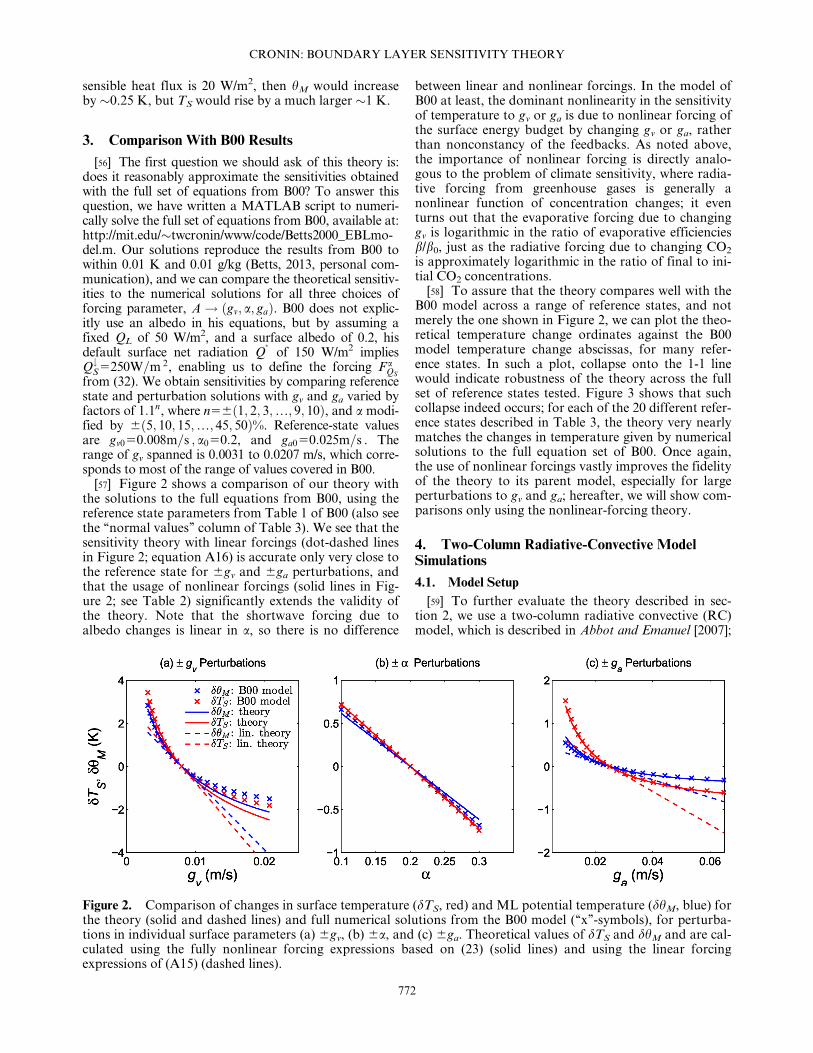
[57] Figure 2 shows a comparison of our theory withthe solutions to the full equations from B00, using thereference state parameters from Table 1 of B00 (also seethe ‘‘normal values’’ column of Table 3). We see that thesensitivity theory with linear forcings (dot-dashed linesin Figure 2; equation A16) is accurate only very close tothe reference state for 6gv and 6ga perturbations, andthat the usage of nonlinear forcings (solid lines in Fig-ure 2; see Table 2) significantly extends the validity ofthe theory. Note that the shortwave forcing due toalbedo changes is linear in a, so there is no difference

between linear and nonlinear forcings. In the model ofB00 at least, the dominant nonlinearity in the sensitivityof temperature to gv or ga is due to nonlinear forcing ofthe surface energy budget by changing gv or ga, ratherthan nonconstancy of the feedbacks. As noted above,the importance of nonlinear forcing is directly analo-gous to the problem of climate sensitivity, where radia-tive forcing from greenhouse gases is generally anonlinear function of concentration changes; it eventurns out that the evaporative forcing due to changinggv is logarithmic in the ratio of evaporative efficienciesb/b0, just as the radiative forcing due to changing CO2

is approximately logarithmic in the ratio of final to ini-tial CO2 concentrations.

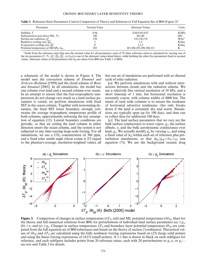
[58] To assure that the theory compares well with theB00 model across a range of reference states, and notmerely the one shown in Figure 2, we can plot the theo-retical temperature change ordinates against the B00model temperature change abscissas, for many refer-ence states. In such a plot, collapse onto the 1-1 linewould indicate robustness of the theory across the fullset of reference states tested. Figure 3 shows that suchcollapse indeed occurs; for each of the 20 different refer-ence states described in Table 3, the theory very nearlymatches the changes in temperature given by numericalsolutions to the full equation set of B00. Once again,the use of nonlinear forcings vastly improves the fidelityof the theory to its parent model, especially for largeperturbations to gv and ga; hereafter, we will show com-parisons only using the nonlinear-forcing theory.

4. Two-Column Radiative-Convective ModelSimulations

4.1. Model Setup

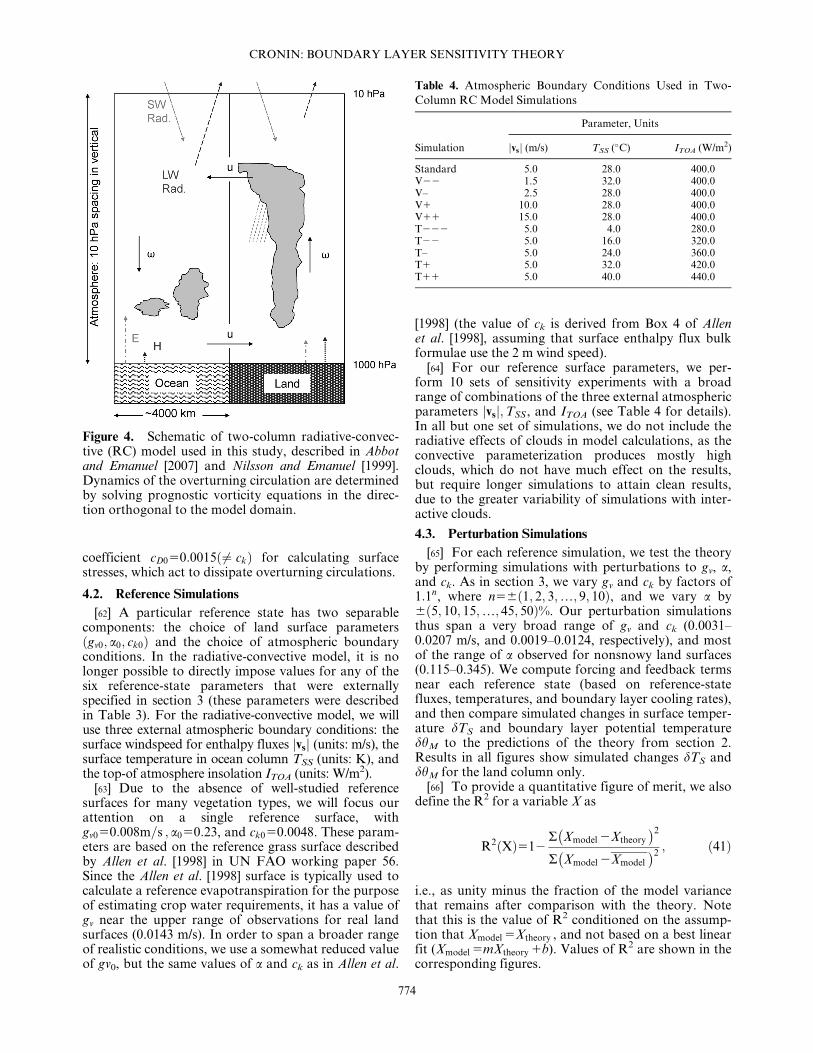
[59] To further evaluate the theory described in sec-tion 2, we use a two-column radiative convective (RC)model, which is described in Abbot and Emanuel [2007];

Figure 2. Comparison of changes in surface temperature (dTS, red) and ML potential temperature (dhM, blue) forthe theory (solid and dashed lines) and full numerical solutions from the B00 model (‘‘x’’-symbols), for perturba-tions in individual surface parameters (a) 6gv, (b) 6a, and (c) 6ga. Theoretical values of dTS and dhM and are cal-culated using the fully nonlinear forcing expressions based on (23) (solid lines) and using the linear forcingexpressions of (A15) (dashed lines).

CRONIN: BOUNDARY LAYER SENSITIVITY THEORY

772

a schematic of the model is shown in Figure 4. Themodel uses the convection scheme of Emanuel andZivkovic-Rothman [1999] and the cloud scheme of Bonyand Emanuel [2001]. In all simulations, the model hasone column over land and a second column over ocean.In an attempt to ensure that the free-tropospheric tem-peratures do not change very much as a land surface pa-rameter is varied, we perform simulations with fixedSST in the ocean column. Together with nonrotating dy-namics, the fixed SST lower boundary strongly con-strains the average tropospheric temperature profile ofboth columns, approximately enforcing the key assump-tion of equation (12). Lateral boundary conditions areperiodic, so that air exiting the land column in eitherdirection enters the ocean column, and the system is notsubjected to any time-varying large-scale forcing. For allsimulations, we use a CO2 concentration of 360 ppm,and a fixed solar zenith angle whose cosine is 2/3 (equalto the planetary-average, insolation-weighted value); all

but one set of simulations are performed with no diurnalcycle of solar radiation.

[60] We perform simulations with and without inter-actions between clouds and the radiation scheme. Weuse a relatively fine vertical resolution of 10 hPa, and ashort timestep of 1 min, but horizontal resolution isextremely coarse, with column widths of 4000 km. Theintent of such wide columns is to ensure the weaknessof horizontal advective tendencies—this only breaksdown if the land is extremely dry and warm. Simula-tions are typically spun up for 100 days, and then runto collect data for additional 100 days.

[61] The land surface parameters that we vary are thebulk surface conductance to water vapor, gv, the surfacealbedo, a, and the bulk aerodynamic conductance overland, ga. We actually modify ga by varying ck, and usinga fixed value of jvsj within each set of reference plus per-turbation simulations, so that dga=ga05dck=ck0 (seeequation (7)). We use the background oceanic drag

Table 3. Reference-State Parameters Used in Comparison of Theory and Solutions to Full Equation Set of B00 (Figure 3)a

Parameter Normal Value Alternate Values Units

Stability, C 0.06 0.04,0.05,0.07 K/hPaSubsaturation just above ML, PT 100 60,140 hPaSurface net radiation, Q

�150 110,130,170 W/m2

Radiative cooling rate, QR 3 1,2 K/dayEvaporative cooling rate, QC 0 1,2,3 K/dayPotential temperature at 940 hPa, h00 303 283,288,293,298,308,313 K

aAside from the reference state that uses the normal value for all parameters, each of 19 other reference states is calculated by varying one ofthe six parameters (C;PT ;Q�;QR ;QC , or h00) to one of the alternate values listed below, while holding the other five parameters fixed at normalvalues. Alternate values of all parameters but h00 are taken from B00 (see Table 1 of B00).

Figure 3. Comparison of changes in surface temperature (dTS, red) and ML potential temperature (dhM, blue) forthe theory and full numerical solutions from B00, for perturbations of individual land surface parameters (a) 6gv,(b) 6a, and (c) 6ga. Changes in surface temperature dTS and boundary layer potential temperature dhM are com-puted from the full equation set of B00 (abscissas) and based on the theory of section 2 (ordinates). Theoretical val-ues of dhM and dTS are calculated using the fully nonlinear forcing expressions based on (23) (large solid points)and using the linear forcing expressions of (A15) (small points). A 1-1 line is drawn in black on each subfigure forreference, and each subfigure includes points from 20 reference states, each with 20 perturbations to gv,a, or ga—see text and Table 3 for details.

CRONIN: BOUNDARY LAYER SENSITIVITY THEORY

773

coefficient cD050:0015 6¼ ckð Þ for calculating surfacestresses, which act to dissipate overturning circulations.

4.2. Reference Simulations

[62] A particular reference state has two separablecomponents: the choice of land surface parametersgv0; a0; ck0ð Þ and the choice of atmospheric boundary

conditions. In the radiative-convective model, it is nolonger possible to directly impose values for any of thesix reference-state parameters that were externallyspecified in section 3 (these parameters were describedin Table 3). For the radiative-convective model, we willuse three external atmospheric boundary conditions: thesurface windspeed for enthalpy fluxes jvsj (units: m/s), thesurface temperature in ocean column TSS (units: K), andthe top-of atmosphere insolation ITOA (units: W/m2).

[63] Due to the absence of well-studied referencesurfaces for many vegetation types, we will focus ourattention on a single reference surface, withgv050:008m=s ; a050:23, and ck050:0048. These param-eters are based on the reference grass surface describedby Allen et al. [1998] in UN FAO working paper 56.Since the Allen et al. [1998] surface is typically used tocalculate a reference evapotranspiration for the purposeof estimating crop water requirements, it has a value ofgv near the upper range of observations for real landsurfaces (0.0143 m/s). In order to span a broader rangeof realistic conditions, we use a somewhat reduced valueof gv0, but the same values of a and ck as in Allen et al.

[1998] (the value of ck is derived from Box 4 of Allenet al. [1998], assuming that surface enthalpy flux bulkformulae use the 2 m wind speed).

[64] For our reference surface parameters, we per-form 10 sets of sensitivity experiments with a broadrange of combinations of the three external atmosphericparameters jvsj;TSS, and ITOA (see Table 4 for details).In all but one set of simulations, we do not include theradiative effects of clouds in model calculations, as theconvective parameterization produces mostly highclouds, which do not have much effect on the results,but require longer simulations to attain clean results,due to the greater variability of simulations with inter-active clouds.

4.3. Perturbation Simulations

[65] For each reference simulation, we test the theoryby performing simulations with perturbations to gv, a,and ck. As in section 3, we vary gv and ck by factors of1:1n, where n56 1; 2; 3;…; 9; 10ð Þ, and we vary a by6 5; 10; 15;…; 45; 50ð Þ%. Our perturbation simulationsthus span a very broad range of gv and ck (0.0031–0.0207 m/s, and 0.0019–0.0124, respectively), and mostof the range of a observed for nonsnowy land surfaces(0.115–0.345). We compute forcing and feedback termsnear each reference state (based on reference-statefluxes, temperatures, and boundary layer cooling rates),and then compare simulated changes in surface temper-ature dTS and boundary layer potential temperaturedhM to the predictions of the theory from section 2.Results in all figures show simulated changes dTS anddhM for the land column only.

[66] To provide a quantitative figure of merit, we alsodefine the R2 for a variable X as

R2 Xð Þ512R Xmodel 2Xtheory

� �2

R Xmodel 2Xmodel

� �2; ð41Þ

i.e., as unity minus the fraction of the model variancethat remains after comparison with the theory. Notethat this is the value of R2 conditioned on the assump-tion that Xmodel 5Xtheory , and not based on a best linearfit (Xmodel 5mXtheory 1b). Values of R2 are shown in thecorresponding figures.

Figure 4. Schematic of two-column radiative-convec-tive (RC) model used in this study, described in Abbotand Emanuel [2007] and Nilsson and Emanuel [1999].Dynamics of the overturning circulation are determinedby solving prognostic vorticity equations in the direc-tion orthogonal to the model domain.

Table 4. Atmospheric Boundary Conditions Used in Two-

Column RC Model Simulations

Simulation

Parameter, Units

jvsj (m/s) TSS (�C) ITOA (W/m2)

Standard 5.0 28.0 400.0V22 1.5 32.0 400.0V– 2.5 28.0 400.0V1 10.0 28.0 400.0V11 15.0 28.0 400.0T222 5.0 4.0 280.0T22 5.0 16.0 320.0T– 5.0 24.0 360.0T1 5.0 32.0 420.0T11 5.0 40.0 440.0

CRONIN: BOUNDARY LAYER SENSITIVITY THEORY

774

4.4. Results

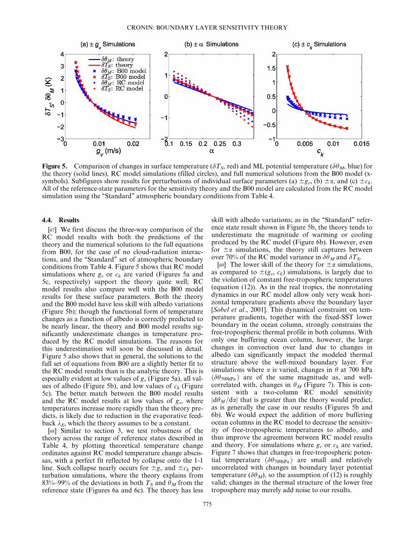
[67] We first discuss the three-way comparison of theRC model results with both the predictions of thetheory and the numerical solutions to the full equationsfrom B00, for the case of no cloud-radiation interac-tions, and the ‘‘Standard’’ set of atmospheric boundaryconditions from Table 4. Figure 5 shows that RC modelsimulations where gv or ck are varied (Figures 5a and5c, respectively) support the theory quite well; RCmodel results also compare well with the B00 modelresults for these surface parameters. Both the theoryand the B00 model have less skill with albedo variations(Figure 5b); though the functional form of temperaturechanges as a function of albedo is correctly predicted tobe nearly linear, the theory and B00 model results sig-nificantly underestimate changes in temperature pro-duced by the RC model simulations. The reasons forthis underestimation will soon be discussed in detail.Figure 5 also shows that in general, the solutions to thefull set of equations from B00 are a slightly better fit tothe RC model results than is the analytic theory. This isespecially evident at low values of gv (Figure 5a), all val-ues of albedo (Figure 5b), and low values of ck (Figure5c). The better match between the B00 model resultsand the RC model results at low values of gv, wheretemperatures increase more rapidly than the theory pre-dicts, is likely due to reduction in the evaporative feed-back kE, which the theory assumes to be a constant.

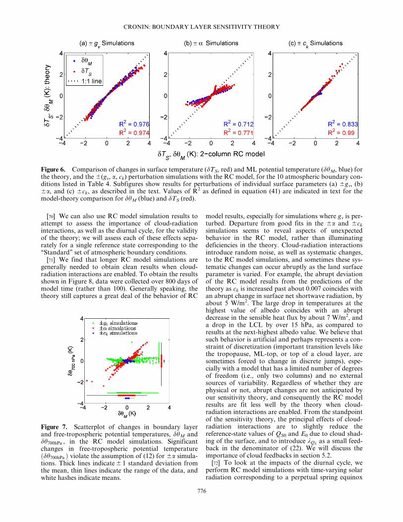
[68] Similar to section 3, we test robustness of thetheory across the range of reference states described inTable 4, by plotting theoretical temperature changeordinates against RC model temperature change abscis-sas, with a perfect fit reflected by collapse onto the 1-1line. Such collapse nearly occurs for 6gv and 6ck per-turbation simulations, where the theory explains from83%–99% of the deviations in both TS and hM from thereference state (Figures 6a and 6c). The theory has less

skill with albedo variations; as in the ‘‘Standard’’ refer-ence state result shown in Figure 5b, the theory tends tounderestimate the magnitude of warming or coolingproduced by the RC model (Figure 6b). However, evenfor 6a simulations, the theory still captures betweenover 70% of the RC model variance in dhM and dTS.

[69] The lower skill of the theory for 6a simulations,as compared to 6(gv, ck) simulations, is largely due tothe violation of constant free-tropospheric temperatures(equation (12)). As in the real tropics, the nonrotatingdynamics in our RC model allow only very weak hori-zontal temperature gradients above the boundary layer[Sobel et al., 2001]. This dynamical constraint on tem-perature gradients, together with the fixed-SST lowerboundary in the ocean column, strongly constrains thefree-tropospheric thermal profile in both columns. Withonly one buffering ocean column, however, the largechanges in convection over land due to changes inalbedo can significantly impact the modeled thermalstructure above the well-mixed boundary layer. Forsimulations where a is varied, changes in h at 700 hPadh700hPað Þ are of the same magnitude as, and well-

correlated with, changes in hM (Figure 7). This is con-sistent with a two-column RC model sensitivityjdhM=daj that is greater than the theory would predict,as is generally the case in our results (Figures 5b and6b). We would expect the addition of more bufferingocean columns in the RC model to decrease the sensitiv-ity of free-tropospheric temperatures to albedo, andthus improve the agreement between RC model resultsand theory. For simulations where gv or ck are varied,Figure 7 shows that changes in free-tropospheric poten-tial temperature dh700hPað Þ are small and relativelyuncorrelated with changes in boundary layer potentialtemperature (dhM), so the assumption of (12) is roughlyvalid; changes in the thermal structure of the lower freetroposphere may merely add noise to our results.

Figure 5. Comparison of changes in surface temperature (dTS, red) and ML potential temperature (dhM, blue) forthe theory (solid lines), RC model simulations (filled circles), and full numerical solutions from the B00 model (x-symbols). Subfigures show results for perturbations of individual surface parameters (a) 6gv, (b) 6a, and (c) 6ck.All of the reference-state parameters for the sensitivity theory and the B00 model are calculated from the RC modelsimulation using the ‘‘Standard’’ atmospheric boundary conditions from Table 4.

CRONIN: BOUNDARY LAYER SENSITIVITY THEORY

775

[70] We can also use RC model simulation results toattempt to assess the importance of cloud-radiationinteractions, as well as the diurnal cycle, for the validityof the theory; we will assess each of these effects sepa-rately for a single reference state corresponding to the‘‘Standard’’ set of atmospheric boundary conditions.

[71] We find that longer RC model simulations aregenerally needed to obtain clean results when cloud-radiation interactions are enabled. To obtain the resultsshown in Figure 8, data were collected over 800 days ofmodel time (rather than 100). Generally speaking, thetheory still captures a great deal of the behavior of RC

model results, especially for simulations where gv is per-turbed. Departure from good fits in the 6a and 6ck

simulations seems to reveal aspects of unexpectedbehavior in the RC model, rather than illuminatingdeficiencies in the theory. Cloud-radiation interactionsintroduce random noise, as well as systematic changes,to the RC model simulations, and sometimes these sys-tematic changes can occur abruptly as the land surfaceparameter is varied. For example, the abrupt deviationof the RC model results from the predictions of thetheory as ck is increased past about 0.007 coincides withan abrupt change in surface net shortwave radiation, byabout 5 W/m2. The large drop in temperatures at thehighest value of albedo coincides with an abruptdecrease in the sensible heat flux by about 7 W/m2, anda drop in the LCL by over 15 hPa, as compared toresults at the next-highest albedo value. We believe thatsuch behavior is artificial and perhaps represents a con-straint of discretization (important transition levels likethe tropopause, ML-top, or top of a cloud layer, aresometimes forced to change in discrete jumps), espe-cially with a model that has a limited number of degreesof freedom (i.e., only two columns) and no externalsources of variability. Regardless of whether they arephysical or not, abrupt changes are not anticipated byour sensitivity theory, and consequently the RC modelresults are fit less well by the theory when cloud-radiation interactions are enabled. From the standpointof the sensitivity theory, the principal effects of cloud-radiation interactions are to slightly reduce thereference-state values of QS0 and E0 due to cloud shad-ing of the surface, and to introduce kQS

as a small feed-back in the denominator of (22). We will discuss theimportance of cloud feedbacks in section 5.2.

[72] To look at the impacts of the diurnal cycle, weperform RC model simulations with time-varying solarradiation corresponding to a perpetual spring equinox

Figure 6. Comparison of changes in surface temperature (dTS, red) and ML potential temperature (dhM, blue) forthe theory, and the 6(gv, a, ck) perturbation simulations with the RC model, for the 10 atmospheric boundary con-ditions listed in Table 4. Subfigures show results for perturbations of individual surface parameters (a) 6gv, (b)6a, and (c) 6ck, as described in the text. Values of R2 as defined in equation (41) are indicated in text for themodel-theory comparison for dhM (blue) and dTS (red).

Figure 7. Scatterplot of changes in boundary layerand free-tropospheric potential temperatures, dhM anddh700hPa , in the RC model simulations. Significantchanges in free-tropospheric potential temperaturedh700hPað Þ violate the assumption of (12) for 6a simula-

tions. Thick lines indicate 6 1 standard deviation fromthe mean, thin lines indicate the range of the data, andwhite hashes indicate means.

CRONIN: BOUNDARY LAYER SENSITIVITY THEORY

776

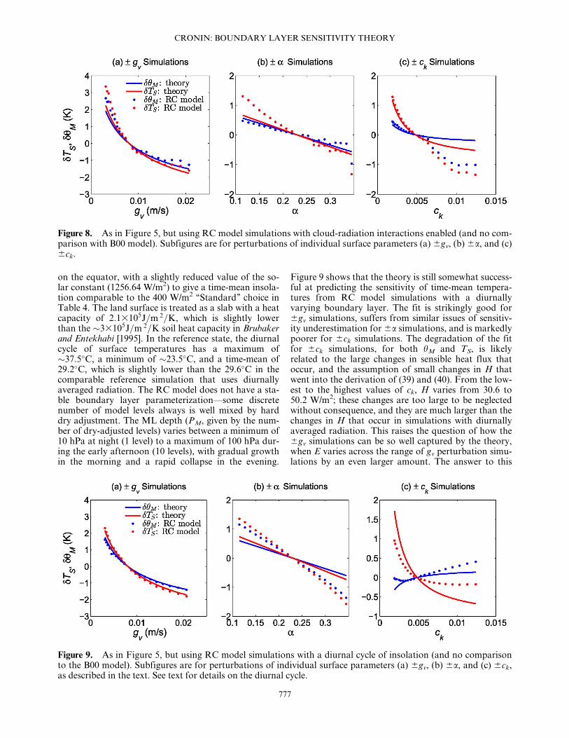
on the equator, with a slightly reduced value of the so-lar constant (1256.64 W/m2) to give a time-mean insola-tion comparable to the 400 W/m2 ‘‘Standard’’ choice inTable 4. The land surface is treated as a slab with a heatcapacity of 2:13105J=m 2=K, which is slightly lowerthan the �33105J=m 2=K soil heat capacity in Brubakerand Entekhabi [1995]. In the reference state, the diurnalcycle of surface temperatures has a maximum of�37.5�C, a minimum of �23.5�C, and a time-mean of29.2�C, which is slightly lower than the 29.6�C in thecomparable reference simulation that uses diurnallyaveraged radiation. The RC model does not have a sta-ble boundary layer parameterization—some discretenumber of model levels always is well mixed by harddry adjustment. The ML depth (PM, given by the num-ber of dry-adjusted levels) varies between a minimum of10 hPa at night (1 level) to a maximum of 100 hPa dur-ing the early afternoon (10 levels), with gradual growthin the morning and a rapid collapse in the evening.

Figure 9 shows that the theory is still somewhat success-ful at predicting the sensitivity of time-mean tempera-tures from RC model simulations with a diurnallyvarying boundary layer. The fit is strikingly good for6gv simulations, suffers from similar issues of sensitiv-ity underestimation for 6a simulations, and is markedlypoorer for 6ck simulations. The degradation of the fitfor 6ck simulations, for both hM and TS, is likelyrelated to the large changes in sensible heat flux thatoccur, and the assumption of small changes in H thatwent into the derivation of (39) and (40). From the low-est to the highest values of ck, H varies from 30.6 to50.2 W/m2; these changes are too large to be neglectedwithout consequence, and they are much larger than thechanges in H that occur in simulations with diurnallyaveraged radiation. This raises the question of how the6gv simulations can be so well captured by the theory,when E varies across the range of gv perturbation simu-lations by an even larger amount. The answer to this

Figure 8. As in Figure 5, but using RC model simulations with cloud-radiation interactions enabled (and no com-parison with B00 model). Subfigures are for perturbations of individual surface parameters (a) 6gv, (b) 6a, and (c)6ck.

Figure 9. As in Figure 5, but using RC model simulations with a diurnal cycle of insolation (and no comparisonto the B00 model). Subfigures are for perturbations of individual surface parameters (a) 6gv, (b) 6a, and (c) 6ck,as described in the text. See text for details on the diurnal cycle.

CRONIN: BOUNDARY LAYER SENSITIVITY THEORY

777

question likely lies in the covariance of E and kE, whichmakes the term E= kH1kE1kQL

� �more constant than

either its numerator or denominator.

5. Discussion

[73] We believe that the results from sections 3 and 4generally show the theory to be a useful tool by whichto understand the sensitivity of the equilibrium bound-ary layer over land. However, it is worth taking a stepback to discuss some of the important limitations andopen questions that relate to the applicability of ourresults.

5.1. Limitations of the Theory

[74] Neglect of horizontal advection is a major limita-tion of the theory, and restricts our attention to regionsthat are large enough in spatial scale, and weak enoughin horizontal gradients, for horizontal advective tenden-cies to be unimportant in the ML. Brubaker and Ente-khabi [1995] suggest that thermal advection may beunimportant for regions with roughly homogeneoussurface conditions that span areas of �104 to 105 km2,though horizontal moisture advection is alwaysrequired to balance the water budget in their model. Tothe extent that the flow in a thermally driven, linearlydamped low-level circulation scales with the tempera-ture gradient [e.g., Nilsson and Emanuel, 1999, Section3c], such circulations generate an advective coolingtendency that scales as the square of the temperaturegradient. Thus, if ML temperature gradients in the ref-erence state are weak, a linear sensitivity analysisshould ignore changes in horizontal advective coolingas a higher-order term— dhMð Þ2—in the ML thermalbalance. An interesting subject for future work wouldbe to study how the ML response scales with the hori-zontal scale of the forcing, which would be relevant for

understanding the applicability of the theory to real-world changes in land surface properties.

[75] Another significant limitation, as alluded toabove, is the oversimplified treatment of the sensitivityof ML thermal balance involved in deriving (14). A fulltreatment of the change in ML thermal balance requiresdifferentiation of the total ML cooling PMQR

� �:

d

dAPMQR� �

5 QR01QC0

� � dPM

dA1PM0

dQR

dA1

dQC

dA

:

ð42Þ

[76] We can quantify the relative importance ofchanges in ML thickness versus ML average coolingrates by looking at the logarithmic derivative of (42):

d

dAln PMQR� �

5P21M0

dPM

dA1QR0

21 dQR

dA1QR0

21 dQC

dA

ð43Þ

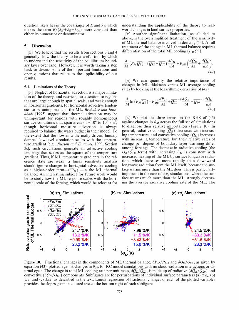
[77] We plot the three terms on the RHS of (43)against changes in hM across the full set of simulationsto diagnose their relative importances (Figure 10). Ingeneral, radiative cooling QR

� �decreases with increas-

ing temperature, and convective cooling QC

� �increases

with increasing temperature, but their relative rates ofchange per degree of boundary layer warming differamong forcings. The decrease in radiative cooling (theQR=QR0 term) with increasing hM is consistent withincreased heating of the ML by surface longwave radia-tion, which increases more rapidly than downwardlongwave radiation from the ML itself, because the sur-face warms more than the ML does. This is particularlyimportant in the case of 6ck simulations, where the sur-face warms much more than the ML, strongly decreas-ing the average radiative cooling rate of the ML. The

Figure 10. Fractional changes in the components of ML thermal balance, dPM=PM0 and dQR=QR0 , as given byequation (43), plotted against changes in hM, for RC model simulations with no cloud-radiation interactions or di-urnal cycle. The change in total ML cooling rate per unit mass, dQR=QR0 , is made up of radiative dQR=QR0

� �and

convective dQC=QR0

� �components. Subfigures are for perturbations of individual surface parameters (a) 6gv, (b)

6a, and (c) 6ck, as described in the text. Linear regression of fractional changes of each of the plotted variablesprovides the slopes given in colored text at the bottom right of each subfigure.

CRONIN: BOUNDARY LAYER SENSITIVITY THEORY

778

increase in convective cooling (the QC=QR0 term) withincreasing hM is consistent with more evaporation ofrain in a deeper, drier ML. Only in the case of 6gv sim-ulations do changes in ML depth (the dPM=PM0 term)dominate changes in cooling rate of the ML, whichhelps to explain why 6gv simulations are fit best by thetheory. Ultimately, these significant deviations fromconstant ML cooling rate do not present an insur-mountable problem for the validity of our theory,because the constant cooling rate assumption is largelyembedded in the value of c. Despite the appearance of cin a number of places throughout the theory, it rarelydominates the full expression for the sensitivity of TS orhM, since it is generally small (�0.2) compared to thefactor of 1 to which it is added in the expression for kE.For the 6a simulations, the nontrivial changes in habove the ML (as discussed in section 4.3) help toexplain why dPM=PM0 in Figure 10b has a lower slopeas a function of dhM than in Figures 10a and 10c. A sig-nificant part of the change in hM for the 6a simulationsis unrelated to changes in PM and occurs simply due towarming of the lower free troposphere.

[78] Another limitation is less visible in the simulationresults we have shown but has somewhat constrainedour exploration of parameter space. Generally speak-ing, the key assumption of a constant hT profile is vio-lated in the RC model if there is an abrupt changebetween deep convection and no deep convection in onecolumn or the other; with similar but more dramaticresults than the abrupt changes that were shown whencloud-radiation interactions were enabled. In order toattempt to avoid such cases (which we view as some-what artificial, related to discretization and the limitednumber of columns), we have filtered our results foractive deep convection in both columns (as diagnosedby a significantly nonzero time-mean updraft mass fluxat 700 hPa), and we have also attempted to choose pa-rameters and reference states that ensure some deepconvection in both columns. This requirement unfortu-nately limits the accessibility of surfaces with very lowvalues of gv, which would theoretically have high sensi-tivity to further drying (or other surface parameterchanges).

[79] The assumption of a constant hT profile, includ-ing constant C, also prevents the theory from beingapplied in its present state to perturbations that causewarming or cooling, or affect the lapse rate, of the freetroposphere. This means that changes in ML structuredue to the long-term effects of CO2 as a global green-house gas will not be captured by the theory we havepresented. Sensitivity of boundary layer temperaturesto free-tropospheric temperatures is an important prob-lem not only from the standpoint of climate change butalso from a standpoint of understanding how thecoupled surface-ML system acts to amplify or dampensynoptic variability, as in heat waves. In its currentform, the theory may be useful for understanding thefast component of CO2-driven greenhouse warming,where land warms but sea surface temperatures remainnearly fixed [Dong et al., 2009; Wyant et al., 2012]. Sincesuch warming is driven by a simple longwave radiative

perturbation to the surface energy budget, we could cal-culate the theoretical response by simply plugging in thesurface longwave radiative forcing of a step change inCO2 to the general sensitivity equation (22). As we willdiscuss later, the theory may also be useful for under-standing the nonradiative implications of changes inCO2 on the surface energy balance (i.e., physiologicalforcing). It is possible to modify the theory to allow forforcings that impact the free-tropospheric temperatureprofile, by modifying equation (15) to include a term@hT=@A. We have not included this term because itmakes the subsequent derivation more algebraicallycumbersome (dqM=dA is no longer related to dhM=dAby a simple multiplicative factor) than is consideredworthwhile for this paper. The calculation of equilib-rium boundary layer sensitivity to free-tropospherictemperature represents less an inherent limitation oftheory than an opportunity for future valuable work.

[80] A final limitation of the theory is likely evident:by using as the basis for our theory an equilibriummodel with diurnally averaged solar forcing, we do nottake into account any nonlinearities associated with thediurnal cycle, which could alter the quantitative sensi-tivities of the time-mean thermal structure of theboundary layer to the time-mean of the surface fluxes.This might occur in a meaningful way for our theory,for example, if forcings and feedbacks covaried in time(over the course of the day) significantly enough thatthe covariance terms were large compared to the time-mean terms (our theory considers only the time-meanterms). As noted by B00, it appears that the equilibriummixed layer model can explain a substantial amount ofthe variability in daily-average surface temperaturesacross two basins in the midwestern United States, sothere is reason to hope that diurnal nonlinearities arenot overwhelming. We have also shown that the sensi-tivity theory still appears to compare favorably with thetime-mean solutions from RC model simulationsobtained with diurnally varying radiation, though thetheory as applied to 6a and 6ck simulations hasreduced skill (Figure 9). The similarity of the climaticand diurnal cycle equilbria from Brubaker and Ente-khabi [1995] lends additional support to the hypothesisthat diurnal nonlinearities are not of critical importancefor daily-average temperatures. While these are allencouraging signs, neither our simulations with diur-nally varying radiation nor the work of Brubaker andEntekhabi [1995] adequately parameterizes many im-portant aspects of the stable nocturnal boundary layer.The importance of diurnal nonlinearities for our theory,especially those associated with the stable nocturnalboundary layer, remains an important and open ques-tion for future research.

5.2. Precipitation, Convection, and Clouds

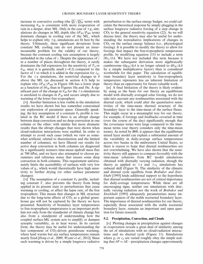
[81] Plotting changes in precipitation against changesin evaporation reveals a great deal of similarity amongthe set of simulations with no cloud-radiation interac-tions and no diurnal cycle (Figure 11). Simulationswhere gv or ck are varied roughly obey the simple scal-ing that dP � dE—precipitation changes approximately

CRONIN: BOUNDARY LAYER SENSITIVITY THEORY

779

equal evaporation changes. This rough equality holdsbecause changes in moisture convergence by the two-column overturning circulation are small for 6gv and6ck simulations. Rough equality of changes in precipi-tation and evaporation fails to hold for 6a simulations,where dP changes much more rapidly than dE. Changesin land surface albedo affect atmospheric columnenergy balance, and thus the moisture converged byoverturning circulations, much more strongly than dochanges in surface roughness or vegetation conduct-ance. Figure 11 also helps to show the typical scales ofsensitivity of precipitation to the three land surface pa-rameters. Changes in precipitation are quite small for6ck simulations, intermediate for 6gv simulations, andlarge for 6a simulations, with the standard deviation ofrdP � 0.1, 0.5, and 1.5 mm/d for the three surface pa-rameters, respectively (averaged across all atmosphericboundary conditions).

[82] In simulations where albedo is varied, subcloudquasiequilibrium [Raymond, 1995] provides a usefultheory with which to diagnose changes in cumulus massfluxes and, to some extent, precipitation rates. Specifi-cally, we expect that the updraft mass flux at cloud baseMu should equal the large-scale vertical mass flux atcloud base, 2x/g, plus a term related to the surfacefluxes divided by the column-average saturation staticenergy (SSE) deficit:

Mu52x=g1H1E

b h�2h� � : ð44Þ

[83] Here, b is an unknown factor relating the averageSSE deficit in the free troposphere, h�2h, to the averageSSE deficit in downdrafts. With b � 2, the RHS andLHS of (44) agree, as diagnosed from model output. In

simulations with varying albedo, we find empiricallythat we can diagnose changes in precipitation by theapproximation:

dP � d MuqMð Þ: ð45Þ

[84] In other words, for 6a simulations, changes inprecipitation, dP, appear to scale with changes in theproduct of cloud base mass flux (Mu)—itself dependenton the total turbulent surface enthalpy flux H 1 E via44—and boundary layer specific humidity (qM).

[85] The RC model simulations with interactionsbetween clouds and radiation allow us to estimate theshortwave feedback kQS

, and to understand whetherour null assumption regarding it has significantlyaffected our theory. We diagnose kQS

by linear regres-sion of dQS against dhM (correcting for any changes inQS that are due to changes in a). We find that short-wave feedbacks are a modest but significant positivefeedback for 6gv and 6ck simulations but a stronglynegative feedback for 6a simulations. A linear modeldQS5kQS

dhM explains the vast majority (80–95%) ofthe variance in dQS, and gives kQS

� 16:8;ð236:5;18:6ÞW=m 2=K, for 6 gv; a; ckð Þ simulations,respectively. These results suggest that warming due toreduced gv or ck leads to less cloudiness and that warm-ing due to decreased a leads to more cloudiness.Clearly, the concept of forcing-independent feedbacksdoes not apply in the case of kQS

. For both gv and ck,the inferred values for kQS

are considerably smaller thanthe typical values of kE, so the theory still captures mostof the variance in dhM and dTS, even with the assump-tion kQS

50. For a, the value of kQSis quite large, and

would tend to make changes in hM smaller than ourtheory would predict with kQS

50. We instead see theopposite bias: our theory underestimates the magnitudeof dhM in Figure 8 because of the compensating effectsof free-tropospheric temperature changes in 6a simula-tions, a somewhat fortuitous cancellation. These resultsregarding shortwave effects of cloud changes warrantsome skepticism, because there is no separate parame-terization of shallow cumulus convection in the model;it is likely unrealistic that simulated changes in netshortwave radiation occur principally due to changes indeep clouds.

5.3. Applications

[86] The theory presented here potentially has broadquantitative applications to changes in climate drivenby land cover changes. Whether land cover change isanthropogenic or natural, it will almost invariablyresult in concurrent changes in conductance to watervapor, albedo, and surface roughness. Here we will dis-cuss one application, to the subject of changes in cli-mate driven by stomatal closure under elevated CO2,which has been termed ‘‘physiological forcing’’ of CO2

by Betts et al. [2004] and others [e.g., Boucher et al.,2009; Cao et al., 2009, 2010; Betts and Chiu, 2010;Andrews et al., 2011].

[87] Numerous experimental studies have found thatstomata, the pores in the leaves of plants through which

Figure 11. Scatterplot of changes in precipitation (dP,mm/day) against changes in evaporation (dE, mm/day)for RC model simulations with no cloud-radiationinteractions or diurnal cycle. The black diagonal lineindicates dP 5 dE, which is followed roughly for 6gv

and 6ck simulations, but not 6a simulations, whereprecipitation changes much more rapidly than evapora-tion due to changes in overturning circulation strength.

CRONIN: BOUNDARY LAYER SENSITIVITY THEORY

780

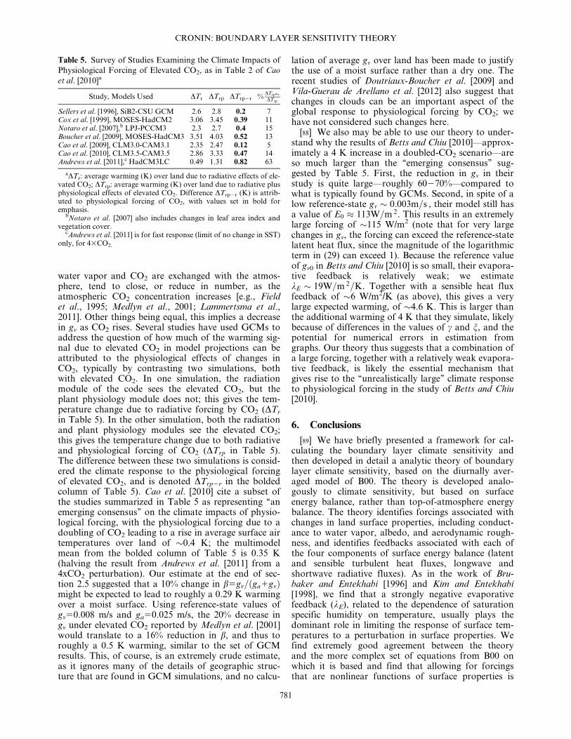
water vapor and CO2 are exchanged with the atmos-phere, tend to close, or reduce in number, as theatmospheric CO2 concentration increases [e.g., Fieldet al., 1995; Medlyn et al., 2001; Lammertsma et al.,2011]. Other things being equal, this implies a decreasein gv as CO2 rises. Several studies have used GCMs toaddress the question of how much of the warming sig-nal due to elevated CO2 in model projections can beattributed to the physiological effects of changes inCO2, typically by contrasting two simulations, bothwith elevated CO2. In one simulation, the radiationmodule of the code sees the elevated CO2, but theplant physiology module does not; this gives the tem-perature change due to radiative forcing by CO2 (DTr

in Table 5). In the other simulation, both the radiationand plant physiology modules see the elevated CO2;this gives the temperature change due to both radiativeand physiological forcing of CO2 (DTrp in Table 5).The difference between these two simulations is consid-ered the climate response to the physiological forcingof elevated CO2, and is denoted DTrp2r in the boldedcolumn of Table 5). Cao et al. [2010] cite a subset ofthe studies summarized in Table 5 as representing ‘‘anemerging consensus’’ on the climate impacts of physio-logical forcing, with the physiological forcing due to adoubling of CO2 leading to a rise in average surface airtemperatures over land of �0.4 K; the multimodelmean from the bolded column of Table 5 is 0.35 K(halving the result from Andrews et al. [2011] from a4xCO2 perturbation). Our estimate at the end of sec-tion 2.5 suggested that a 10% change in b5gv= ga1gvð Þmight be expected to lead to roughly a 0.29 K warmingover a moist surface. Using reference-state values ofgv50.008 m/s and ga50.025 m/s, the 20% decrease ingv under elevated CO2 reported by Medlyn et al. [2001]would translate to a 16% reduction in b, and thus toroughly a 0.5 K warming, similar to the set of GCMresults. This, of course, is an extremely crude estimate,as it ignores many of the details of geographic struc-ture that are found in GCM simulations, and no calcu-

lation of average gv over land has been made to justifythe use of a moist surface rather than a dry one. Therecent studies of Doutriaux-Boucher et al. [2009] andVila-Guerau de Arellano et al. [2012] also suggest thatchanges in clouds can be an important aspect of theglobal response to physiological forcing by CO2; wehave not considered such changes here.

[88] We also may be able to use our theory to under-stand why the results of Betts and Chiu [2010]—approx-imately a 4 K increase in a doubled-CO2 scenario—areso much larger than the ‘‘emerging consensus’’ sug-gested by Table 5. First, the reduction in gv in theirstudy is quite large—roughly 60270%—compared towhat is typically found by GCMs. Second, in spite of alow reference-state gv � 0:003m=s , their model still hasa value of E0 � 113W=m 2. This results in an extremelylarge forcing of �115 W/m2 (note that for very largechanges in gv, the forcing can exceed the reference-statelatent heat flux, since the magnitude of the logarithmicterm in (29) can exceed 1). Because the reference valueof gv0 in Betts and Chiu [2010] is so small, their evapora-tive feedback is relatively weak; we estimatekE � 19W=m 2=K. Together with a sensible heat fluxfeedback of �6 W/m2/K (as above), this gives a verylarge expected warming, of �4.6 K. This is larger thanthe additional warming of 4 K that they simulate, likelybecause of differences in the values of c and n, and thepotential for numerical errors in estimation fromgraphs. Our theory thus suggests that a combination ofa large forcing, together with a relatively weak evapora-tive feedback, is likely the essential mechanism thatgives rise to the ‘‘unrealistically large’’ climate responseto physiological forcing in the study of Betts and Chiu[2010].

6. Conclusions

[89] We have briefly presented a framework for cal-culating the boundary layer climate sensitivity andthen developed in detail a analytic theory of boundarylayer climate sensitivity, based on the diurnally aver-aged model of B00. The theory is developed analo-gously to climate sensitivity, but based on surfaceenergy balance, rather than top-of-atmosphere energybalance. The theory identifies forcings associated withchanges in land surface properties, including conduct-ance to water vapor, albedo, and aerodynamic rough-ness, and identifies feedbacks associated with each ofthe four components of surface energy balance (latentand sensible turbulent heat fluxes, longwave andshortwave radiative fluxes). As in the work of Bru-baker and Entekhabi [1996] and Kim and Entekhabi[1998], we find that a strongly negative evaporativefeedback (kE), related to the dependence of saturationspecific humidity on temperature, usually plays thedominant role in limiting the response of surface tem-peratures to a perturbation in surface properties. Wefind extremely good agreement between the theoryand the more complex set of equations from B00 onwhich it is based and find that allowing for forcingsthat are nonlinear functions of surface properties is

Table 5. Survey of Studies Examining the Climate Impacts of

Physiological Forcing of Elevated CO2, as in Table 2 of Cao

et al. [2010]a

Study, Models Used DTr DTrp DTrp2r %DTrp-r

DTrp

Sellers et al. [1996], SiB2-CSU GCM 2.6 2.8 0.2 7Cox et al. [1999], MOSES-HadCM2 3.06 3.45 0.39 11Notaro et al. [2007],b LPJ-PCCM3 2.3 2.7 0.4 15Boucher et al. [2009], MOSES-HadCM3 3.51 4.03 0.52 13Cao et al. [2009], CLM3.0-CAM3.1 2.35 2.47 0.12 5Cao et al. [2010], CLM3.5-CAM3.5 2.86 3.33 0.47 14Andrews et al. [2011],c HadCM3LC 0.49 1.31 0.82 63

aDTr: average warming (K) over land due to radiative effects of ele-vated CO2; DTrp: average warming (K) over land due to radiative plusphysiological effects of elevated CO2. Difference DTrp2r (K) is attrib-uted to physiological forcing of CO2, with values set in bold foremphasis.

bNotaro et al. [2007] also includes changes in leaf area index andvegetation cover.

cAndrews et al. [2011] is for fast response (limit of no change in SST)only, for 43CO2.

CRONIN: BOUNDARY LAYER SENSITIVITY THEORY

781

key to obtaining good agreement for large perturba-tions in surface properties. The importance of nonlin-ear forcings represents an interesting further analogyto climate sensitivity. We have also performed simula-tions with a two-column RC model with many moredegrees of freedom, which supports the general utilityof the theory even when many of the assumptionsupon which it is based are no longer strictly enforced.

[90] Although the theory has a number of limitations,we believe that it may be broadly useful for unifyingour understanding of how changes in land use or eco-system function may affect changes in climate. As anexample case, we explore the application of the theoryto the problem of climate change driven by suppressionof surface conductance to water vapor under elevatedCO2 (physiological forcing). We find that our theoryprovides a reasonable estimate of the warming simu-lated by past studies that have used global models, andmay help to explain why the warming in the simplerstudy of Betts and Chiu [2010] is so large. Directions forfuture work include application to problems such asurbanization, agricultural expansion, and afforestation,as well as extension of the theory to examine forcing byfree-tropospheric temperature change. Even if the quan-titative expressions for feedbacks and forcings pre-sented here prove to be quite different from thosecalculated from GCMs, we hope that the framework ofboundary layer climate sensitivity will help to standard-ize how climate changes induced by land cover changesare assessed in modeling studies.

Appendix A: Details of Sensitivity Theory

A1. Derivation of n

[91] Here, we derive n, the parameter relating changesin qM to changes in hM in equation (20). Expanding (19)gives

dqM

dA5�

pb

@e�

@T

���Tb

dTb

dA2�e� Tbð Þ

p2b

dpb

dA: ðA1Þ

[92] Using (15) and the definition of pb5ps2PM , wecan replace dpb=dA with 2C dhM=dAð Þ. Using the defi-nition of Tb from (18), we have

dTb

dA5

pb

ps

Rcp dhM

dA1

RhM

cppb

dpb

dA

5pb

ps

Rcp

12RhM

cppbC

dhM

dA:

ðA2Þ

[93] Putting this back into (A1) gives

dqM

dA5

@q�

@T

���Tb

pb

ps

Rcp

12RhM

cppbC

1

qM

pbC

" #dhM

dA; ðA3Þ

where we have again used q�5�e�=p and qM5q� Tb; pbð Þto simplify the expression. The term in square bracketsin (A3) is defined as n.

A2. Expansion of Surface Energy Balance

[94] The total derivatives in (4) can be expanded bythe chain rule

dQS

dA5@QS

@A1@QS

@TS

dTS

dA1@QS

@hM

dhM

dA1@QS

@qM

dqM

dAðA4Þ

dQL

dA5@QL

@A1@QL

@TS

dTS

dA1@QL

@hM

dhM

dA1@QL

@qM

dqM

dAðA5Þ

dH

dA5@H

@A1@H

@TS

dTS

dA1@H

@hM

dhM

dA1@H

@qM

dqM

dAðA6Þ

dE

dA5@E

@A1@E

@TS

dTS

dA1@E

@hM

dhM

dA1@E

@qM

dqM

dA: ðA7Þ

[95] For a typical choice of A, many of these termsvanish, but all are retained here for generality. We caneliminate dTS=dA and dqM=dA from these expressionsin favor of dhM=dA, using (16) and (20). After rearrang-ing to move the differential dA to the right-hand side,this gives

dQS 5@QS

@A2

1

qcpga

@QS

@TS

@H

@A

dA

1 11cð Þ @QS

@TS

1@QS

@hM

1n@QS

@qM

dhM

� dFAQS

1kQSdhM

ðA8Þ

dQL 5@QL

@A2

1

qcpga

@QL

@TS

@H

@A

dA

1 11cð Þ @QL

@TS

1@QL

@hM

1n@QL

@qM

dhM

� dFAQL

1kQLdhM

ðA9Þ

dH 5@H

@A2

1

qcpga

@H

@TS

@H

@A

dA

1 11cð Þ @H

@TS

1@H

@hM

1n@H

@qM

dhM

� dFAH1kHdhM

ðA10Þ

dE 5@E

@A2

1

qcpga

@E

@TS

@H

@A

dA

1 11cð Þ @E

@TS

1@E

@hM

1n@E

@qM

dhM

� dFAE 1kEdhM ;

ðA11Þ

where the terms including a factor of dA (A8)–(A11)have been defined as differential forcings (dFA

QS;

dFAQL; dFA

H , and dFAE ) and the terms multiplying

the differential change in potential temperature, dhM ,have been defined as feedbacks (kQS

; kQL; kH , and kE).

Note that we have kept the symmetry of the equationsfor clarity, but we can make one general simplificationimmediately from the definition of H: dFA

H50, since

CRONIN: BOUNDARY LAYER SENSITIVITY THEORY

782

@H=@TS5qcpga. However, the impacts of @H=@A aredistributed over the other terms dFA

QS; dFA

QL, and dFA

E .[96] Now, applying surface energy balance (3), we can

obtain

dQS2dQL2dH2dE50 ðA12Þ

dFAQS

2dFAQL

2dFAE 1 kQS

2kQL2kH2kE

� �dhM50

ðA13Þ

dFAQS

2dFAQL

2dFAE

kQL1kH1kE2kQS

5dhM ; ðA14Þ

where the last step has assumed the feedbacks are nearlyconstant so that we can rearrange them before integra-tion. Integration of dhM simply yields hM2hM0 � dh.Full integration of the differential forcings gives theresults quoted in the main text, equation (23). We couldalso assume that the forcings were linear inA2A0 � dA, so that

FAQS ;lin

� @QS

@A2

1

qcpga

@QS

@TS

@H

@A

dA

FAQL;lin

� @QL

@A2

1

qcpga

@QL

@TS

@H

@A

dA

FAE;lin �

@E

@A2

1

qcpga

@E

@TS

@H

@A

dA

ðA15Þ

[97] In parallel with the nonlinear-forcing derivationsof sections 2.5–2.7, expressions for total linear forcingswith A! gv; a; gað Þ are given by

Fgv

lin5ga

ga1gv0

E0dgv

gv0

Falin52

QS0

12a0da

Fga

lin5gv

ga01gv

E02H0

Be

dga

ga02

4rBT3S0H0

qcpga0

dga

ga0:

ðA16Þ

[98] For brevity here, we have summed the forcingsfrom different surface fluxes. As discussed in section 3,the usage of linear forcings is generally inferior to theuse of the fully nonlinear forcings described in detail insections 2.5–2.7 and Table 2. We include the expres-sions for linear forcings here to clarify the methodologyunderlying the calculation of the results shown inFigures 2 and 3.

[99] Acknowledgments. I would like to thank Kerry Emanuel formany conversations about this work, as well as for supplying me withthe radiative-convective model on which much of the evaluation of thetheory is based. Peter Molnar, Mike Byrne, Jack Scheff, and twoanonymous reviewers, all provided numerous useful comments andcritiques on various drafts of this work. Alan Betts generously andrapidly shared the quantitative results from Betts [2000], whichallowed for confirmation that my solutions reproduce his. This workwas funded by NSF grant 1136480, The Effect of Near-EquatorialIslands on Climate. Preliminary versions of this work were aided byconversations with Ron Prinn and Adam Schlosser, and funded bygrants from the DOE (DE-FG02–94ER61937) and EPRI (EP-P8155/

C4107), as well as by a supporting research award for the Joint Pro-gram on the Science and Policy of Global Change.

ReferencesAbbot, D., and K. Emanuel (2007), A tropical and subtropical land–

sea–atmosphere drought oscillation mechanism, J. Atmos. Sci., 64,4458–4468, doi:10.1175/2007JAS2186.1.

Allen, R., L. Pereira, D. Raes, and M. Smith (1998), Crop evapotranspi-ration: Guidelines for computing crop water requirements, Irrig.Drain. Pap. 56, 300 pp., United Nations FAO, Rome.

Andrews, T., M. Doutriaux-Boucher, O. Boucher, and P. Forster(2011), A regional and global analysis of carbon dioxide physiologi-cal forcing and its impact on climate, Clim. Dyn., 36, 783–792,doi:10.1007/s00382-010-0742-1.

Betts, A. (2000), Idealized model for equilibrium boundary layer overland, J. Hydrometeorol., 1, 507–523.

Betts, A., and J. Chiu (2010), Idealized model for changes in equilib-rium temperature, mixed layer depth, and boundary layer cloud overland in a doubled CO2 climate, J. Geophys. Res., 115, D19108,doi:10.1029/2009JD012888.

Betts, A., and W. Ridgway (1988), Coupling of the radiative, convec-tive, and surface fluxes over the equatorial pacific, J. Atmos. Sci., 45,522–536.

Betts, A., and W. Ridgway (1989), Climatic equilibrium of the atmos-pheric convective boundary layer over a tropical ocean, J. Atmos.Sci., 46, 2621–2641.

Betts, R., P. Cox, M. Collins, P. Harris, C. Huntingford, and C. Jones(2004), The role of ecosystem-atmosphere interactions in simulatedAmazonian precipitation decrease and forest dieback under globalclimate warming, Theor. Appl. Climatol., 78, 157–175, doi:10.1007/s00704-004-0050-y.

Boucher, O., A. Jones, and R. Betts (2009), Climate response to thephysiological impact of carbon dioxide on plants in the Met OfficeUnified Model HadCM3, Clim. Dyn., 32, 237–249, doi:10.1007/s00382-008-0459-6.

Bony, S., and K. Emanuel (2001), A parameterization of the cloudinessassociated with cumulus convection; Evaluation using TOGACOARE data, J. Atmos. Sci., 58, 3158–3183.

Brubaker, K., and D. Entekhabi (1995), An analytic approach to mod-eling land-atmosphere interaction: 1. Construct and equilibriumbehavior, Water Resour. Res., 31, 619–632.

Brubaker, K., and D. Entekhabi (1996), Analysis of feedback mecha-nisms in land-atmosphere interaction, Water Resour. Res., 32, 1343–1357.

Cao, L., G. Bala, K. Caldeira, R. Nemani, and G. Ban-Weiss (2009),Climate response to physiological forcing of carbon dioxide simu-lated by the coupled community atmosphere model (CAM3.1) andcommunity land model (CLM3.0), Geophys. Res. Lett., 36, L10402,doi:10.1029/2009GL037724.

Cao, L., G. Bala, K. Caldeira, R. Nemani, and G. Ban-Weiss (2010),Importance of carbon dioxide physiological forcing to future climatechange, Proc. Natl. Acad. Sci. U. S. A., 107, 9513–9518, doi:10.1073/pnas.0913000107.

Charney, J. (1975), Dynamics of deserts and drought in the Sahel, Q. J.R. Meteorol. Soc., 101, 193–202.

Cox, P., R. Betts, C. Bunton, R. Essery, P. Rowntree, and J.Smith (1999), The impact of new land surface physics on theGCM simulation of climate and climate sensitivity, Clim. Dyn.,15, 183–203.

Dong, B., J. Gregory, and R. Sutton (2009), Understanding land-seawarming contrast in response to increasing greenhouse gases. Part I:Transient adjustment, J. Clim., 22, 3079–3097, doi:10.1175/2009JCLI2652.1.

Doutriaux-Boucher, M., M. Webb, J. Gregory, and O. Boucher(2009), Carbon dioxide induced stomatal closure increases radiativeforcing via a rapid reduction in low cloud, Geophys. Res. Lett., 36,L02703, doi:10.1029/2008GL036273.

Emanuel, K., and M. Zivkovic-Rothman (1999), Development andevaluation of a convection scheme for use in climate models,J. Atmos. Sci., 56, 1766–1782.

Entekhabi, D., and K. Brubaker (1995), An analytic approach to mod-eling land-atmosphere interaction: 2. Stochastic formulation, WaterResour. Res., 31, 633–643.

CRONIN: BOUNDARY LAYER SENSITIVITY THEORY

783

Field, C., R. Jackson, and H. Mooney (1995), Stomatal responses toincreased CO2: Implications from the plant to the global scale, PlantCell Environ., 18, 1214–1225.

Hartmann, D. (1994), Global Physical Climatology, Int. Geophys. Ser.,vol. 56, 409 pp., Academic Press, San Diego.

Held, I. (2005), The gap between simulation and understanding in cli-mate modeling, Bull. Am. Meteorol. Soc., 80, 1609–1614,doi:10.1175/BAMS-86-11-1609.

Jacobs, C., and H. De Bruin (1992), The sensitivity of regional transpi-ration to land-surface characteristics: Significance of feedback, J.Clim., 5, 683–698.

Jones, H. (1992), Plants and Microclimate, 2nd ed., 428 pp., CambridgeUniv. Press, Cambridge, U.K.

Kim, C., and D. Entekhabi (1998), Feedbacks in the land-surface andmixed-layer energy budgets, Boundary Layer Meteorol., 88, 1–21.

Lammertsma, E., H. de Boer, S. Dekker, D. Dilcher, A. Lotter, and F.Wagner-Cremer (2011), Global CO2 rise leads to reduced maximumstomatal conductance in florida vegetation, Proc. Natl. Acad. Sci. U.S. A., 108, 4035–4040, doi:10.1073/pnas.1100371108.

McNaughton, K., and T. Spriggs (1986), A mixed-layer model for re-gional evaporation, Boundary Layer Meteorol., 34, 243–262.

Medlyn, B., et al. (2001), Stomatal conductance of forest species afterlong-term exposure to elevated CO2 concentration: A synthesis,New Phytolog., 149, 247–264.

Monteith, J. (1965), Evaporation and environment, in The State andMovement of Water in Living Organisms, pp. 205–234, CambridgeUniv. Press, Cambridge, U.K.

Nilsson, J., and K. Emanuel (1999), Equilibrium atmospheres of atwo-column radiative-convective model, Q. J. R. Meteorol. Soc.,125, 2239–2264.

Notaro, M., S. Vavrus, and Z. Liu, (2007), Global vegetation and cli-mate change due to future increases in CO2 as projected by a fullycoupled model with dynamic vegetation, J. Clim., 20, 70–90,doi:10.1175/JCLI3989.1.

Ramaswamy, V., O. Boucher, J. Haigh, D. Haughlustaine, J. Hay-wood, G. Myhre, T. Nakajima, G. Shi, S. Solomon, (2001), Radia-

tive forcing of climate change, in Climate Change 2001: TheScientific Basis. Contribution of Working Group I to the Third Assess-ment Report of the Intergovernmental Panel on Climate Change,edited by J. T. Houghton et al., 881 pp., Cambridge Univ. Press,Cambridge, U. K.

Raymond, D. (1995), Regulation of moist convection over the west pa-cific warm pool, J. Atmos. Sci., 52, 3945–3959.

Sellers, P., et al. (1996), Comparison of radiative and physiological effectsof doubled atmospheric CO2 on climate, Science, 271, 1402–1406.

Shukla, J., and Y. Mintz (1982), Influence of land-surface evapotrans-piration on the Earth’s climate, Science, 215, 1498–1501.

Sobel, A., J. Nilsson, and L. Polvani (2001), The weak temperaturegradient approximation and balanced tropical moisture waves,J. Atmos. Sci., 58, 3650–3665.

Takahashi, K. (2009), Radiative constraints on the hydrological cyclein an idealized radiative-convective equilibrium model, J. Atmos.Sci., 66, 77–91, doi:10.1175/2008JAS2797.1.

Tennekes, H. (1973), A model for the dynamics of the inversion abovea convective boundary layer, J. Atmos. Sci., 30, 558–567.

van Heerwaarden, C., J. Vila-Guerau de Arellano, A. Moene, andA. Holtslag (2009), Interactions between dry-air entrainment, sur-face evaporation and convective boundary-layer development, Q. J.R. Meteorol. Soc., 135, 1277–1291, doi:10.1002/qj.431.

van Heerwaarden, C., J. Vila-Guerau de Arellano, A. Gounou, F. Gui-chard, and F. Couvreux (2010), Understanding the daily cycle ofevapotranspiration: A method to quantify the influence of forcingsand feedbacks, J. Hydrometeorol., 11, 1405–1422, doi:10.1175/2010JHM1272.1.

Vila-Guerau de Arellano, J., C. van Heerwaarden, and J. Lelieveld(2012), Modelled suppression of boundary-layer clouds by plants ina CO2-rich atmosphere, Nat. Geosci., 5, 701–701, doi:10.1038/NGEO1554.

Wyant, C., C. Bretherton, P. Blossey, and M. Khairoutdinov (2012),Fast cloud adjustment to increasing CO2 in a superparameterizedclimate model, J. Adv. Model. Earth Syst., 4, M05001, doi:10.1029/2011MS000092.

CRONIN: BOUNDARY LAYER SENSITIVITY THEORY

784