A semiautomatic method to tie well logs to seismic data

Roberto H. Herrera1 and Mirko van der Baan1

ABSTRACT

We evaluated a semiautomatic method for well-to-seismictying to improve correlation results and reproducibility ofthe procedure. In the manual procedure, the interpreter firstcreates a synthetic trace from edited well logs, determinesthe most appropriate bulk time shift and polarity, and thenapplies a minimum amount of stretching and squeezing tobest match the observed data. The last step resembles a vis-ual pattern recognition task, which often requires some ex-perience. We replaced the last step with a constraineddynamic time-warping technique, to help guide the inter-preter. The method automatically determined the appropriateamount of local stretching and squeezing to produce thehighest correlation between the original data and the createdsynthetic trace. The constraint ensured that stretching andsqueezing were kept within reasonable bounds, as deter-mined by the interpreter. Results compared well with themanual method, leading to ties along the entire trace lengthin contrast to the shorter analysis window in the conven-tional method. Yet, we advise against unsupervised applica-tions because the method is intended as a guide instead of afully automated blind approach.

INTRODUCTION

Tying well logs to seismic traces is a crucial step in seismic in-terpretation to correlate subsurface geology to observed seismicdata. The ease and quality of the tying procedure depend on theavailability of high-quality logs and the estimation of a suitablewavelet. White and Simm (2003) and Newrick (2012) describe bestpractices and general recipes for the tying procedure. An estimatedwavelet is convolved with the reflectivity series calculated from thewell logs (sonic log and bulk density log), to generate the first syn-thetic trace (Anderson and Newrick, 2008). The wavelet can be es-timated directly from the amplitude spectrum of the seismic data,

giving a zero-phase wavelet, which is phase rotated and time shiftedduring the matching process (e.g., White and Simm, 2003) or usinga coherency matching technique (White, 1980; Walden and White,1998), giving a frequency-dependent wavelet. The next step is tomatch the generated synthetic with the seismic data. The target seis-mic trace intuitively should be the trace at the well location, buttime-migration effects could move the best match location awayfrom the well. White and Simm (2003) propose to find the bestmatch time location by scanning several traces in the vicinity ofthe well. Alternatively, as a compensation for dispersion at the welllocation, a composite trace can be generated from the neighboringtraces (e.g., Hampson-Russell, 1999).Well logs are commonly used as ground truth to correlate the

seismic signal with the earth’s stratigraphy (White and Simm,2003), but several key steps render the procedure challengingand rarely fully reproducible. Density logs are greatly affectedby borehole conditions, e.g., washouts or invasion, which nega-tively impact the measurement of the bulk’s rock density (Andersonand Newrick, 2008). On the other hand, sonic logs are less sensitiveto borehole conditions but they are measured at different lengthscales than the seismic data, and thus calibration plays an importantrole via dispersion and check shot corrections. This obviously as-sumes that high-quality velocity and density logs are available; ifnot, pseudocurves have to be estimated by empirical relationships(Newrick, 2012).Only after creation of a first, correctly positioned, synthetic trace

following advocated best practices (White and Simm, 2003) shouldthe actual matching process start. The goal is not to force perfectlymatching waveforms between the synthetic and selected observedtrace, but to find distinctive reflectors on the seismic section that arealso observable on the seismic trace (Newrick, 2012). These reflec-tors are rarely perfectly aligned, for instance, due to dispersion ef-fects, necessitating some corrections in timing. This is done bychanging the sonic velocities by a small amount, i.e., by stretchingor squeezing the synthetic seismogram. The acceptable amount ofimposed interval velocity changes is left to the interpreter’s discre-tion. This particular step is clearly prone to pitfalls due to subjec-tivities in interpretation and procedures. In addition, even the

Manuscript received by the Editor 5 July 2013; revised manuscript received 27 October 2013; published online 12 March 2014.1University of Alberta, Department of Physics, Edmonton, Alberta, Canada. E-mail: rhherrer@ualberta.ca; mirko.vanderbaan@ualberta.ca.© 2014 Society of Exploration Geophysicists. All rights reserved.

V47

GEOPHYSICS, VOL. 79, NO. 3 (MAY-JUNE 2014); P. V47–V54, 8 FIGS.10.1190/GEO2013-0248.1

Dow

nloa

ded

03/1

7/14

to 1

42.2

44.1

91.8

0. R

edis

trib

utio

n su

bjec

t to

SEG

lice

nse

or c

opyr

ight

; see

Ter

ms

of U

se a

t http

://lib

rary

.seg

.org

/

selection of major matching reflections on the synthetic and ob-served traces can be challenging in practice.Furthermore, the quality of the tie between the synthetic and the

seismic trace is based on the correlation coefficient, which is limitedto a constant time-shift similarity. The time-variant nature of theactual propagating wavelet, due to dispersion effects, adds nonli-nearities to the seismic trace that cannot be easily followed by alinear metric. Likewise, nonconsistent dispersion effects in the soniclogs and seismic data affect the estimated reflectivity series, alsoadding time-varying nonlinear variations. We propose to use dy-namic time warping (DTW) to match these time series, wherethe quality of the fit is not limited to the selected correlation windowbut the entire trace. DTW, as a correlation-based technique, mea-sures the goodness of fit but not the reliability of the end results.For that purpose, we use a quality control (QC) step, which isdone by watching the relative velocity changes produced bythe tying.DTW has been proven to handle nonstationarities in signals.

Nonstationarity in time series due to physical processes is commonin many areas such as speech processing (Rabiner and Juang, 1993),medicine, industry, and finance (Keogh, 2002). DTW is a robusttool to match time series even if the shifts vary with time (Keogh,2002).In this work, the application of DTW is limited to the specific

step of stretching and squeezing. This is a controversial (Whiteand Simm, 2003), but necessary, part in the tying procedure.Our procedure substitutes the manual stretching and squeezing stepby an optimization algorithm, which is still supervised by theinterpreter. This improves the repeatability of the tying, whilethe critical and often-abused stretch and squeeze (Newrick,2012) is still under control. We assume that all the best practiceshave been followed (White and Simm, 2003; Anderson and New-rick, 2008).Related works using DTW in seismic applications originate with

attempts to automate well-to-well log correlation (Lineman et al.,1987; Zoraster et al., 2004). Well logs from different wells are cor-related to infer common earth features. Zoraster et al. (2004) findthat the crosscorrelation was unable to follow local distortions suchas stretching or shrinking of stratigraphic intervals, typical of logscollected even from closely spaced wells. Essentially, these meth-ods aim to correlate common features in various logs (Anderson andGaby, 1983). An early approach to DTW is presented by Martinsonet al. (1982) and Martinson and Hopper (1992). They develop amapping function able to track stretching and squeezing in a timeseries, based on a correlation technique to establish a point-for-pointcorrelation between traces. Liner and Clapp (2004) propose a globaloptimization method to create pairwise alignments between seismictraces. More recently, Hale (2013) uses DTW in seismic imageprocessing, which aligns seismic images with differences not lim-ited to time shifts. Our work follows the constrained optimization ofSakoe and Chiba (1978) with DTW, and it is not pairwise, but al-lows for one-to-many connections in both directions between twotraces. We (Herrera and Van der Baan, 2012a) already present anearly stage application, and here we develop a refined and morecomplete method.In this paper, we first explain the theory behind DTW, and then

we introduce the QC parameters. Next, we focus on the practicalimplementation showing a real example. Finally, we discuss ourresults with practical recommendations for application.

THEORY

The conventional method of well ties depends on the quality ofthe matching between the synthetic seismograms with the actualseismic traces. The measure of this matching has been extensivelystudied (e.g., White and Simm, 2003), but it remains based mainlyon linear techniques. We propose the use of dynamic programmingtechniques commonly used in data mining (Keogh and Kasetty,2003; Keogh and Ratanamahatana, 2004) and in speech processing(Rabiner and Juang, 1993).The correlation coefficient is often used to measure the quality

of the seismic-to-well tie (Hampson-Russell, 1999). Comparingtwo (time-dependent) sequences S ¼ ½s1; s2; : : : ; sn� and T ¼½t1; t2; : : : ; tn�, both of length n, gives a correlation coefficient(γST ) at the time lag τ:

γSTðτÞ ¼P

ni¼1½si − μS�½tiþτ − μT �

ðPni¼1 ½si − μS�2

Pni¼1 ½ti − μT �2Þ1∕2

; (1)

where μS and μT are the means of S and T, respectively, and thedenominator supplies the energy normalization term.The optimal time lag τ is generally set at the maximum correla-

tion coefficient. This measure works well if a constant time shift τcharacterizes both signals. When this time alignment is constant, theproblem is reduced to the correction of the time lag by crosscorre-lation. But this measure fails to find the best match in nonstation-ary cases.Most geophysical applications have nonstationary time-align-

ment problems (Anderson and Gaby, 1983). An alternative tothe crosscorrelation is to find the Euclidean distance (L2-norm) be-tween the two time series (Keogh and Kasetty, 2003):

DðS; TÞ ¼ffiffiffiffiffiffiffiffiffiffiffiffiffiffiffiffiffiffiffiffiffiffiffiffiffiXni¼1

ðsi − tiÞ2s

; (2)

where DðS; TÞ is the one-to-one distance between the synthetic Sand the trace T.The Euclidean distance (L2-norm) is the most widely used dis-

tance measure. It is trivial to implement but also is very sensitive tosmall distortions in the time axis (Berndt and Clifford, 1994; Keoghand Kasetty, 2003). Taking the advantages of the Euclidean distanceand adapting it for nonstationary matching, Berndt and Clifford(1994) propose DTW.DTW distance can accommodate stretching and squeezing in the

time series by linear programming. It uses the Euclidean distance asthe initial metric but allows for the one-to-many alignment. Thewarping distance is represented as the minimum path in a grid rep-resentation of both sequences. In Figure 1, the warping path,W ¼ w1; w2; : : : ; wk, aligns the elements of S and T in such away that the distance between them is minimized.In this matrix, the squared distance δ in the elements ði; jÞ is cal-

culated by

δðsi; tjÞ ¼ ðsi − tjÞ2: (3)

To find the best alignment between these two sequences, we have toretrieve the warping path W through the distance matrix thatminimizes the total cumulative distance for each path (Berndtand Clifford, 1994; Keogh, 2002) as illustrated in Figure 1. The

V48 Herrera and van der Baan

Dow

nloa

ded

03/1

7/14

to 1

42.2

44.1

91.8

0. R

edis

trib

utio

n su

bjec

t to

SEG

lice

nse

or c

opyr

ight

; see

Ter

ms

of U

se a

t http

://lib

rary

.seg

.org

/

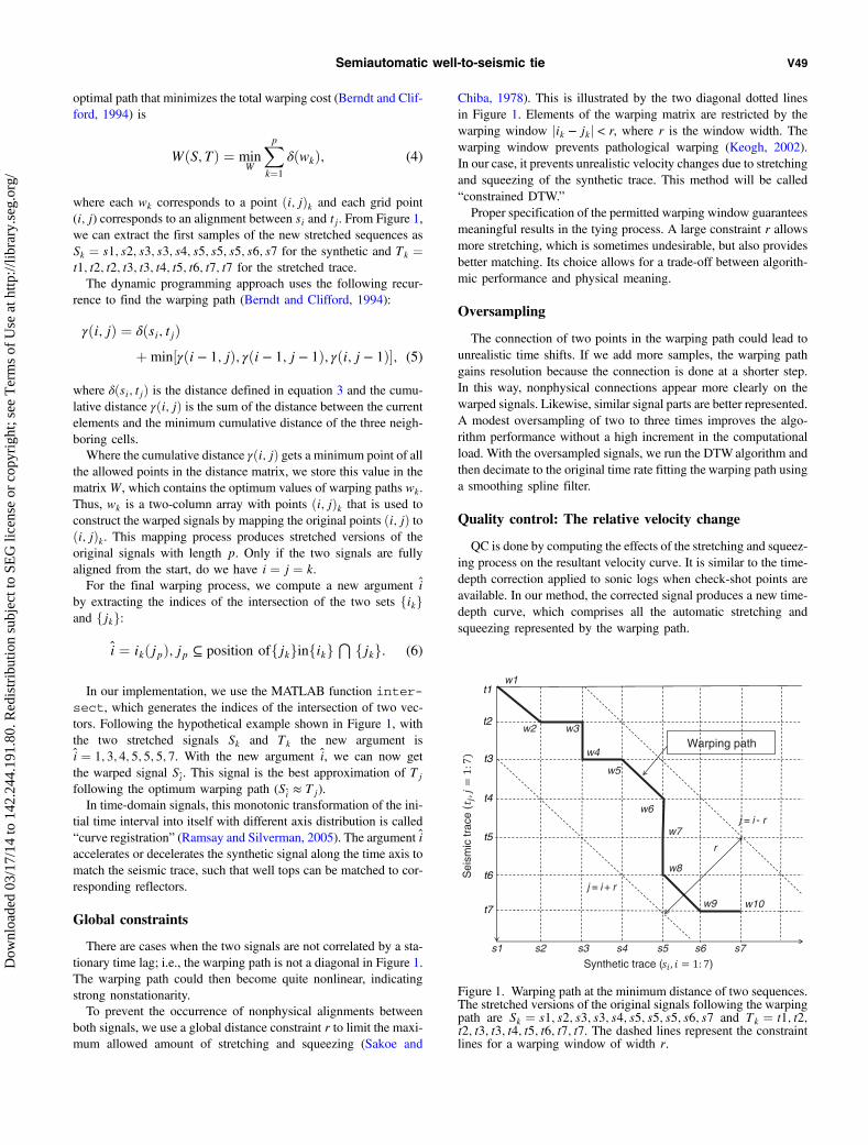
optimal path that minimizes the total warping cost (Berndt and Clif-ford, 1994) is

WðS; TÞ ¼ minW

Xpk¼1

δðwkÞ; (4)

where each wk corresponds to a point ði; jÞk and each grid point(i; j) corresponds to an alignment between si and tj. From Figure 1,we can extract the first samples of the new stretched sequences asSk ¼ s1; s2; s3; s3; s4; s5; s5; s5; s6; s7 for the synthetic and Tk ¼t1; t2; t2; t3; t3; t4; t5; t6; t7; t7 for the stretched trace.The dynamic programming approach uses the following recur-

rence to find the warping path (Berndt and Clifford, 1994):

γði; jÞ ¼ δðsi; tjÞþmin½γði − 1; jÞ; γði − 1; j − 1Þ; γði; j − 1Þ�; (5)

where δðsi; tjÞ is the distance defined in equation 3 and the cumu-lative distance γði; jÞ is the sum of the distance between the currentelements and the minimum cumulative distance of the three neigh-boring cells.Where the cumulative distance γði; jÞ gets a minimum point of all

the allowed points in the distance matrix, we store this value in thematrixW, which contains the optimum values of warping paths wk.Thus, wk is a two-column array with points ði; jÞk that is used toconstruct the warped signals by mapping the original points ði; jÞ toði; jÞk. This mapping process produces stretched versions of theoriginal signals with length p. Only if the two signals are fullyaligned from the start, do we have i ¼ j ¼ k.For the final warping process, we compute a new argument i

by extracting the indices of the intersection of the two sets fikgand fjkg:

i ¼ ikðjpÞ; jp ⊆ position offjkginfikg ⋂ fjkg: (6)

In our implementation, we use the MATLAB function inter-sect, which generates the indices of the intersection of two vec-tors. Following the hypothetical example shown in Figure 1, withthe two stretched signals Sk and Tk the new argument isi ¼ 1; 3; 4; 5; 5; 5; 7. With the new argument i, we can now getthe warped signal Si. This signal is the best approximation of Tj

following the optimum warping path (Si ≈ Tj).In time-domain signals, this monotonic transformation of the ini-

tial time interval into itself with different axis distribution is called“curve registration” (Ramsay and Silverman, 2005). The argument iaccelerates or decelerates the synthetic signal along the time axis tomatch the seismic trace, such that well tops can be matched to cor-responding reflectors.

Global constraints

There are cases when the two signals are not correlated by a sta-tionary time lag; i.e., the warping path is not a diagonal in Figure 1.The warping path could then become quite nonlinear, indicatingstrong nonstationarity.To prevent the occurrence of nonphysical alignments between

both signals, we use a global distance constraint r to limit the maxi-mum allowed amount of stretching and squeezing (Sakoe and

Chiba, 1978). This is illustrated by the two diagonal dotted linesin Figure 1. Elements of the warping matrix are restricted by thewarping window jik − jkj < r, where r is the window width. Thewarping window prevents pathological warping (Keogh, 2002).In our case, it prevents unrealistic velocity changes due to stretchingand squeezing of the synthetic trace. This method will be called“constrained DTW.”Proper specification of the permitted warping window guarantees

meaningful results in the tying process. A large constraint r allowsmore stretching, which is sometimes undesirable, but also providesbetter matching. Its choice allows for a trade-off between algorith-mic performance and physical meaning.

Oversampling

The connection of two points in the warping path could lead tounrealistic time shifts. If we add more samples, the warping pathgains resolution because the connection is done at a shorter step.In this way, nonphysical connections appear more clearly on thewarped signals. Likewise, similar signal parts are better represented.A modest oversampling of two to three times improves the algo-rithm performance without a high increment in the computationalload. With the oversampled signals, we run the DTWalgorithm andthen decimate to the original time rate fitting the warping path usinga smoothing spline filter.

Quality control: The relative velocity change

QC is done by computing the effects of the stretching and squeez-ing process on the resultant velocity curve. It is similar to the time-depth correction applied to sonic logs when check-shot points areavailable. In our method, the corrected signal produces a new time-depth curve, which comprises all the automatic stretching andsqueezing represented by the warping path.

Synthetic trace ( )

Sei

smic

trac

e (

Warping path

j = i + r

j = i - r

t1

s1

w1

w2 w3

w4

w5

w6

w7

w8

w9 w10

t2

t3

t4

t7

r

s2 s3 s4 s5 s6 s7

t5

t6

Figure 1. Warping path at the minimum distance of two sequences.The stretched versions of the original signals following the warpingpath are Sk ¼ s1; s2; s3; s3; s4; s5; s5; s5; s6; s7 and Tk ¼ t1; t2;t2; t3; t3; t4; t5; t6; t7; t7. The dashed lines represent the constraintlines for a warping window of width r.

Semiautomatic well-to-seismic tie V49

Dow

nloa

ded

03/1

7/14

to 1

42.2

44.1

91.8

0. R

edis

trib

utio

n su

bjec

t to

SEG

lice

nse

or c

opyr

ight

; see

Ter

ms

of U

se a

t http

://lib

rary

.seg

.org

/

The ratio of interval (or local) velocity change at depth zi is givenby the derivative of the smoothed warping path w 0ðziÞ for themapped variable i from equation 6. The local change in velocityat depth zi is then Vp;newðziÞ ¼ Vp;oldðziÞ∕w 0ðziÞ.The new time depth curve is then

td;newðziÞ ¼ 2Xi

k¼1

ΔzkVp;newðzkÞ

: (7)

RESULTS

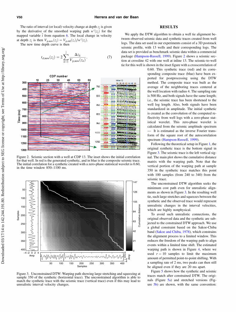
We apply the DTW algorithm to obtain a well tie alignment be-tween observed seismic data and synthetic traces created from welllogs. The data set used in our experiments consist of a 3D poststackseismic profile, with 13 wells and their corresponding logs. Thedata set is provided as benchmark seismic data within a commercialpackage (Hampson-Russell, 1999). Figure 2 shows a seismic sec-tion at crossline 42 with one well at inline 13. The seismic-to-welltie for this well is shown in the inset figure with a crosscorrelation of

0.60. This synthetic trace (red) and its corre-sponding composite trace (blue) have been ex-ported for postprocessing using the DTWmethod. The composite trace was built as theaverage of the neighboring traces centered atthe well location with radius 4. The sampling rateis 500 Hz, and both signals have the same length;i.e., the seismic trace has been shortened to thewell log length. Also, both signals have beenstandardized in amplitude. The initial syntheticis created as the convolution of the computed re-flectivity from well logs with a zero-phase stat-istical wavelet. This zero-phase wavelet iscalculated from the seismic amplitude spectrum— It is estimated as the inverse Fourier trans-form of the square root of the autocorrelationspectrum (Hampson-Russell, 1999).Following the theoretical setup in Figure 1, the

original synthetic trace is the bottom signal inFigure 3. The seismic trace is the left vertical sig-nal. The main plot shows the cumulative distancematrix with the warping path. Note that thevertical portion of the warping path at sample350 in the synthetic trace matches this pointwith 100 samples (from 240 to 340) from theseismic trace.The unconstrained DTW algorithm seeks the

minimum cost path even for unrealistic align-ments as shown in Figure 3. In the resulting welltie, such large stretches and squeezes between thesynthetic and the observed trace would representunrealistic changes in the interval velocities,which are highly nonphysical.To avoid such unrealistic connections, the

original observed data and the synthetic are sub-jected to the constrained DTWapproach. We usea global constraint based on the Sakoe-Chibaband (Sakoe and Chiba, 1978), which constrainsthe alignment process to a limited window. Thisreduces the freedom of the warping path to alignevents within a limited time shift. The estimatedwarping path is shown in Figure 4, where weused r ¼ 10 samples to limit the maximumamount of permitted point-to-point shifting. Witha sampling rate of 2 ms, two peaks can then stillbe aligned even if they are 20 ms apart.Figure 5 shows how the synthetic and seismic

traces match after constrained DTW. The origi-nals (Figure 5a) and stretched versions (Fig-ure 5b) are shown, with the same convention:

Cum

ulat

ive

dist

ance

0

21

42

63

84

105

126

147

−4−2 0 2 4400

350

300

250

200

150

100

50

Sam

ples

Amp

50 100 150 200 250 300 350 400−4−2024

Samples

Am

p

Figure 3. Unconstrained DTW:Warping path showing large stretching and squeezing atsample 350 of the synthetic (horizontal trace). The unconstrained algorithm is able tomatch the synthetic trace with the seismic trace (vertical trace) even if this may lead tounrealistic interval velocity changes.

Figure 2. Seismic section with a well at CDP 13. The inset shows the initial correlationfor that well. In red is the generated synthetic, and in blue is the composite seismic trace.The initial correlation for a synthetic created with a zero-phase statistical wavelet is 0.60,in the time window 850–1100 ms.

V50 Herrera and van der Baan

Dow

nloa

ded

03/1

7/14

to 1

42.2

44.1

91.8

0. R

edis

trib

utio

n su

bjec

t to

SEG

lice

nse

or c

opyr

ight

; see

Ter

ms

of U

se a

t http

://lib

rary

.seg

.org

/

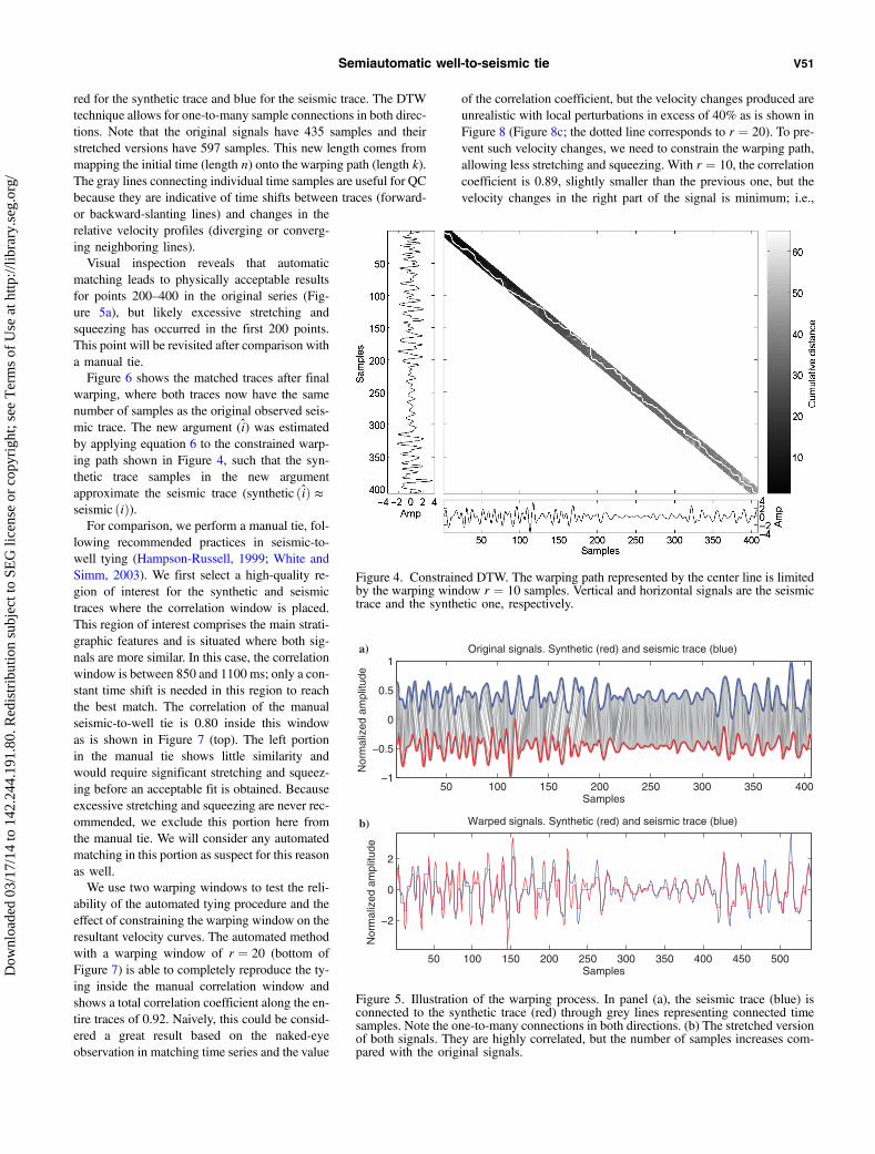
red for the synthetic trace and blue for the seismic trace. The DTWtechnique allows for one-to-many sample connections in both direc-tions. Note that the original signals have 435 samples and theirstretched versions have 597 samples. This new length comes frommapping the initial time (length n) onto the warping path (length k).The gray lines connecting individual time samples are useful for QCbecause they are indicative of time shifts between traces (forward-or backward-slanting lines) and changes in therelative velocity profiles (diverging or converg-ing neighboring lines).Visual inspection reveals that automatic

matching leads to physically acceptable resultsfor points 200–400 in the original series (Fig-ure 5a), but likely excessive stretching andsqueezing has occurred in the first 200 points.This point will be revisited after comparison witha manual tie.Figure 6 shows the matched traces after final

warping, where both traces now have the samenumber of samples as the original observed seis-mic trace. The new argument (i) was estimatedby applying equation 6 to the constrained warp-ing path shown in Figure 4, such that the syn-thetic trace samples in the new argumentapproximate the seismic trace (synthetic ðiÞ ≈seismic ðiÞ).For comparison, we perform a manual tie, fol-

lowing recommended practices in seismic-to-well tying (Hampson-Russell, 1999; White andSimm, 2003). We first select a high-quality re-gion of interest for the synthetic and seismictraces where the correlation window is placed.This region of interest comprises the main strati-graphic features and is situated where both sig-nals are more similar. In this case, the correlationwindow is between 850 and 1100 ms; only a con-stant time shift is needed in this region to reachthe best match. The correlation of the manualseismic-to-well tie is 0.80 inside this windowas is shown in Figure 7 (top). The left portionin the manual tie shows little similarity andwould require significant stretching and squeez-ing before an acceptable fit is obtained. Becauseexcessive stretching and squeezing are never rec-ommended, we exclude this portion here fromthe manual tie. We will consider any automatedmatching in this portion as suspect for this reasonas well.We use two warping windows to test the reli-

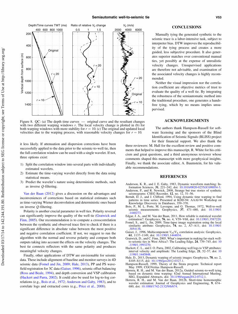
ability of the automated tying procedure and theeffect of constraining the warping window on theresultant velocity curves. The automated methodwith a warping window of r ¼ 20 (bottom ofFigure 7) is able to completely reproduce the ty-ing inside the manual correlation window andshows a total correlation coefficient along the en-tire traces of 0.92. Naively, this could be consid-ered a great result based on the naked-eyeobservation in matching time series and the value

of the correlation coefficient, but the velocity changes produced areunrealistic with local perturbations in excess of 40% as is shown inFigure 8 (Figure 8c; the dotted line corresponds to r ¼ 20). To pre-vent such velocity changes, we need to constrain the warping path,allowing less stretching and squeezing. With r ¼ 10, the correlationcoefficient is 0.89, slightly smaller than the previous one, but thevelocity changes in the right part of the signal is minimum; i.e.,

Figure 4. Constrained DTW. The warping path represented by the center line is limitedby the warping window r ¼ 10 samples. Vertical and horizontal signals are the seismictrace and the synthetic one, respectively.

50 100 150 200 250 300 350 400−1

−0.5

0

0.5

1Original signals. Synthetic (red) and seismic trace (blue)

Nor

mal

ized

am

plitu

de

Samples

50 100 150 200 250 300 350 400 450 500

−2

0

2

Warped signals. Synthetic (red) and seismic trace (blue)

Nor

mal

ized

am

plitu

de

Samples

a)

b)

Figure 5. Illustration of the warping process. In panel (a), the seismic trace (blue) isconnected to the synthetic trace (red) through grey lines representing connected timesamples. Note the one-to-many connections in both directions. (b) The stretched versionof both signals. They are highly correlated, but the number of samples increases com-pared with the original signals.

Semiautomatic well-to-seismic tie V51

Dow

nloa

ded

03/1

7/14

to 1

42.2

44.1

91.8

0. R

edis

trib

utio

n su

bjec

t to

SEG

lice

nse

or c

opyr

ight

; see

Ter

ms

of U

se a

t http

://lib

rary

.seg

.org

/

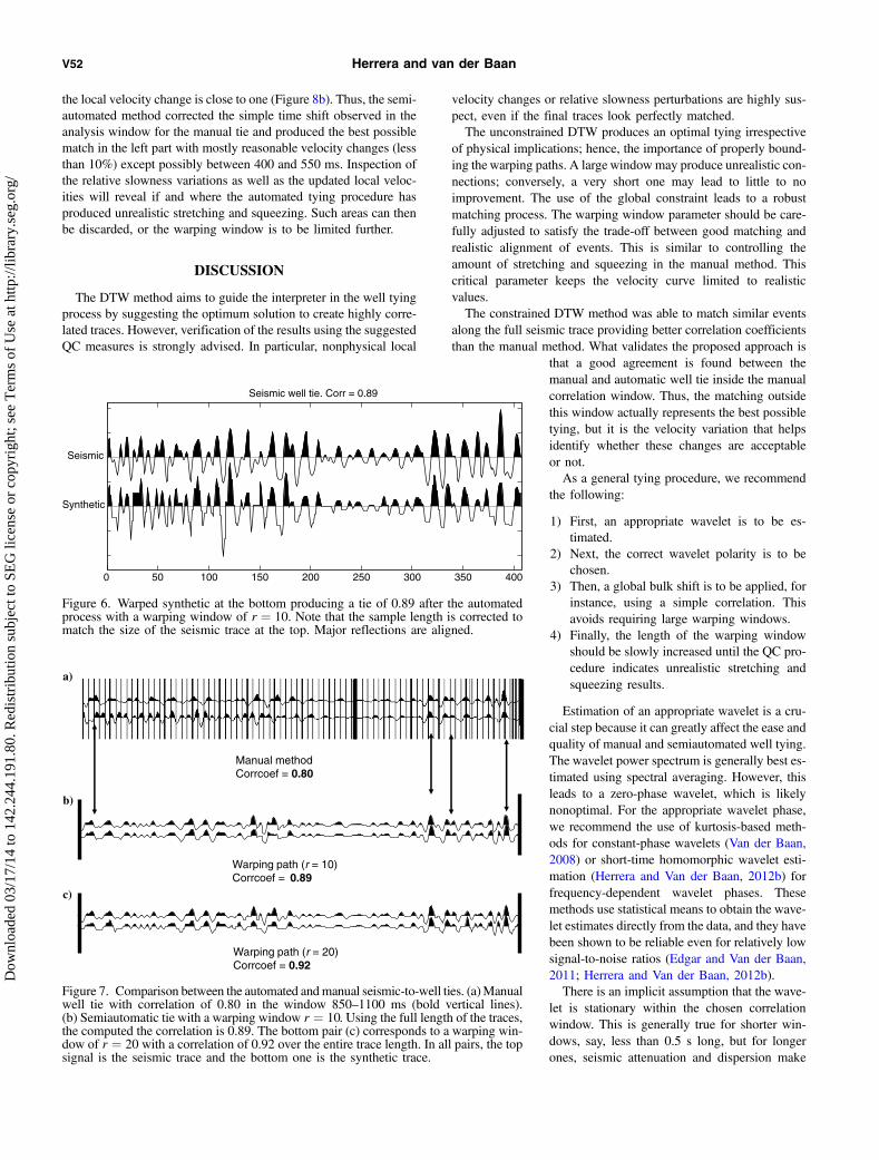
the local velocity change is close to one (Figure 8b). Thus, the semi-automated method corrected the simple time shift observed in theanalysis window for the manual tie and produced the best possiblematch in the left part with mostly reasonable velocity changes (lessthan 10%) except possibly between 400 and 550 ms. Inspection ofthe relative slowness variations as well as the updated local veloc-ities will reveal if and where the automated tying procedure hasproduced unrealistic stretching and squeezing. Such areas can thenbe discarded, or the warping window is to be limited further.

DISCUSSION

The DTW method aims to guide the interpreter in the well tyingprocess by suggesting the optimum solution to create highly corre-lated traces. However, verification of the results using the suggestedQC measures is strongly advised. In particular, nonphysical local

velocity changes or relative slowness perturbations are highly sus-pect, even if the final traces look perfectly matched.The unconstrained DTW produces an optimal tying irrespective

of physical implications; hence, the importance of properly bound-ing the warping paths. A large windowmay produce unrealistic con-nections; conversely, a very short one may lead to little to noimprovement. The use of the global constraint leads to a robustmatching process. The warping window parameter should be care-fully adjusted to satisfy the trade-off between good matching andrealistic alignment of events. This is similar to controlling theamount of stretching and squeezing in the manual method. Thiscritical parameter keeps the velocity curve limited to realisticvalues.The constrained DTW method was able to match similar events

along the full seismic trace providing better correlation coefficientsthan the manual method. What validates the proposed approach is

that a good agreement is found between themanual and automatic well tie inside the manualcorrelation window. Thus, the matching outsidethis window actually represents the best possibletying, but it is the velocity variation that helpsidentify whether these changes are acceptableor not.As a general tying procedure, we recommend

the following:

1) First, an appropriate wavelet is to be es-timated.

2) Next, the correct wavelet polarity is to bechosen.

3) Then, a global bulk shift is to be applied, forinstance, using a simple correlation. Thisavoids requiring large warping windows.

4) Finally, the length of the warping windowshould be slowly increased until the QC pro-cedure indicates unrealistic stretching andsqueezing results.

Estimation of an appropriate wavelet is a cru-cial step because it can greatly affect the ease andquality of manual and semiautomated well tying.The wavelet power spectrum is generally best es-timated using spectral averaging. However, thisleads to a zero-phase wavelet, which is likelynonoptimal. For the appropriate wavelet phase,we recommend the use of kurtosis-based meth-ods for constant-phase wavelets (Van der Baan,2008) or short-time homomorphic wavelet esti-mation (Herrera and Van der Baan, 2012b) forfrequency-dependent wavelet phases. Thesemethods use statistical means to obtain the wave-let estimates directly from the data, and they havebeen shown to be reliable even for relatively lowsignal-to-noise ratios (Edgar and Van der Baan,2011; Herrera and Van der Baan, 2012b).There is an implicit assumption that the wave-

let is stationary within the chosen correlationwindow. This is generally true for shorter win-dows, say, less than 0.5 s long, but for longerones, seismic attenuation and dispersion make

Synthetic

Seismic

0 50 100 150 200 250 300 350 400

Seismic well tie. Corr = 0.89

Figure 6. Warped synthetic at the bottom producing a tie of 0.89 after the automatedprocess with a warping window of r ¼ 10. Note that the sample length is corrected tomatch the size of the seismic trace at the top. Major reflections are aligned.

Manual method Corrcoef = 0.80

Warping path (r = 10)Corrcoef = 0.89

Warping path (r = 20)Corrcoef = 0.92

a)

b)

c)

Figure 7. Comparison between the automated andmanual seismic-to-well ties. (a)Manualwell tie with correlation of 0.80 in the window 850–1100 ms (bold vertical lines).(b) Semiautomatic tie with a warping window r ¼ 10. Using the full length of the traces,the computed the correlation is 0.89. The bottom pair (c) corresponds to a warping win-dow of r ¼ 20 with a correlation of 0.92 over the entire trace length. In all pairs, the topsignal is the seismic trace and the bottom one is the synthetic trace.

V52 Herrera and van der Baan

Dow

nloa

ded

03/1

7/14

to 1

42.2

44.1

91.8

0. R

edis

trib

utio

n su

bjec

t to

SEG

lice

nse

or c

opyr

ight

; see

Ter

ms

of U

se a

t http

://lib

rary

.seg

.org

/

it less likely. If attenuation and dispersion corrections have beensuccessfully applied to the data prior to the seismic-to-well tie, thenthe full correlation window can be used with a single wavelet. If not,three options exist:

1) Split the correlation window into several parts with individuallyestimated wavelets.

2) Estimate the time-varying wavelet directly from the data usingstatistical means.

3) Predict the wavelet’s nature using deterministic methods, suchas inverse Q-filtering.

Van der Baan (2012) gives a discussion on the advantages andinconveniences of corrections based on statistical estimates suchas time-varying Wiener deconvolution and deterministic ones basedon inverse Q-filtering.Polarity is another crucial parameter in well ties. Polarity reversal

can significantly improve the quality of the well tie (Gratwick andFinn, 2005). Our recommendation is to compute a crosscorrelationbetween the synthetic and observed trace first to check if there is asignificant difference in absolute value between the most positiveand negative correlation coefficient. If not, we suggest to run thealgorithm with the normal and reverse polarity and compare bothoutputs taking into account the effects on the velocity changes. Thebest tie connects reflectors with the same polarity and producesmeaningful velocity changes.Finally, other applications of DTW are envisionable for seismic

data. These include alignment of baseline and monitor surveys in 4Dseismic data (Fomel and Jin, 2009; Hale, 2013), PP and PS wave-field registration for 3C data (Gaiser, 1996), seismic offset balancing(Ross and Beale, 1994), and depth conversion and VSP calibration(Hackert and Parra, 2002). It could also be used for log-to-log cor-relations (e.g., Bois et al., 1972; Anderson and Gaby, 1983), and tocorrelate logs and extracted cores (e.g., Price et al., 2008).

CONCLUSIONS

Manually tying the generated synthetic to theseismic trace is a labor-intensive task, subject tointerpreter bias. DTW improves the reproducibil-ity of the tying process and creates a moreguided, less subjective procedure. It also gener-ates superior matches over conventional manualties, yet possibly at the expense of unrealisticvelocity changes. Unsupervised applicationsare therefore not advisable, and examination ofthe associated velocity changes is highly recom-mended.Neither the visual impression nor the correla-

tion coefficient are objective metrics of trust toevaluate the quality of a well tie. By integratingthe robustness of the semiautomatic method intothe traditional procedure, one generates a hands-free tying, which by no means implies unsu-pervised.

ACKNOWLEDGMENTS

The authors thank Hampson-Russell for soft-ware licensing and the sponsors of the BlindIdentification of Seismic Signals (BLISS) projectfor their financial support. We also thank the

three reviewers: M. Hall for the excellent review and positive com-ments that helped to improve this manuscript, R. White for his criti-cism and great questions, and a third anonymous reviewer whosecomments shaped this manuscript with more geophysical insights.Finally, we thank the associate editor, A. Baumstein, for his valu-able recommendations.

REFERENCES

Anderson, K. R., and J. E. Gaby, 1983, Dynamic waveform matching: In-formation Sciences, 31, 221–242, doi: 10.1016/0020-0255(83)90054-3.

Anderson, P., and R. Newrick, 2008, Strange but true stories of syntheticseismograms: CSEG Recorder, 12, no. 12, 51–56.

Berndt, D. J., and J. Clifford, 1994, Using dynamic time warping to findpatterns in time series: Presented at KDD-94: AAAI-94 Workshop onKnowledge Discovery in Databases, 359–370.

Bois, P., M. L. Porte, M. Lavergne, and G. Thomas, 1972, Well-to-wellseismic measurements: Geophysics, 37, 471–480, doi: 10.1190/1.1440273.

Edgar, J. A., and M. Van der Baan, 2011, How reliable is statistical waveletestimation?: Geophysics, 76, no. 4, V59–V68, doi: 10.1190/1.3587220.

Fomel, S., and L. Jin, 2009, Time-lapse image registration using the localsimilarity attribute: Geophysics, 74, no. 2, A7–A11, doi: 10.1190/1.3054136.

Gaiser, J., 1996, Multicomponent VP∕VS correlation analysis: Geophysics,61, 1137–1149, doi: 10.1190/1.1444034.

Gratwick, D., and C. Finn, 2005, What’s important in making far-stack well-to-seismic ties in West Africa?: The Leading Edge, 24, 739–745, doi: 10.1190/1.1993270.

Hackert, C. L., and J. O. Parra, 2002, Calibrating well logs to VSP attributes:interval velocity and amplitude: The Leading Edge, 21, 52–57, doi: 10.1190/1.1445848.

Hale, D., 2013, Dynamic warping of seismic images: Geophysics, 78, no. 2,S105–S115, doi: 10.1190/geo2012-0327.1.

Hampson-Russell, 1999, Theory of the Strata program: Technical reportMay 1999, CGGVeritas Hampson-Russell.

Herrera, R. H., and M. Van der Baan, 2012a, Guided seismic-to-well tyingbased on dynamic time warping: 82nd Annual International Meeting,SEG, Expanded Abstracts, doi: 10.1190/segam2012-0712.1.

Herrera, R. H., and M. Van der Baan, 2012b, Short-time homomorphicwavelet estimation: Journal of Geophysics and Engineering, 9, 674–680, doi: 10.1088/1742-2132/9/6/674.

400 600 800 1000200

400

600

800

1000

1200

1400

Depth/Time curves TWT (ms)V

ertic

al d

epth

from

sur

face

(m

)

0.5 1 1.5

Ratio of relative VP change

2000 4000 6000

VP (m/s)

Original

r = 10

r = 20

r = 10

r = 20

Original

r = 10

r = 20

Figure 8. QC: (a) The depth time curves — original curve and the resultant changeswith two different warping windows r. The local velocity change is plotted in (b) forboth warping windows with more stability for r ¼ 10. (c) The original and updated localvelocities due to the warping process, with reasonable velocity changes for r ¼ 10.

Semiautomatic well-to-seismic tie V53

Dow

nloa

ded

03/1

7/14

to 1

42.2

44.1

91.8

0. R

edis

trib

utio

n su

bjec

t to

SEG

lice

nse

or c

opyr

ight

; see

Ter

ms

of U

se a

t http

://lib

rary

.seg

.org

/

Keogh, E., 2002, Exact indexing of dynamic time warping, in P. A.Bernstein, Y. E. Ioannidis, R. Ramakrishnan, and D. Papadias, eds., Pro-ceedings of the 28th International Conference on Very Large Data Bases,VLDB Endowment, Morgan Kaufman, 406–417.

Keogh, E., and S. Kasetty, 2003, On the need for time series data miningbenchmarks: A survey and empirical demonstration: Data Mining andKnowledge Discovery, 7, 349–371, doi: 10.1023/A:1024988512476.

Keogh, E., and C. A. Ratanamahatana, 2004, Exact indexing of dynamictime warping: Knowledge and Information Systems, 7, 358–386, doi:10.1007/s10115-004-0154-9.

Lineman, D., J. Mendelson, and M. Toksoz, 1987, Well to well logcorrelation using knowledge-based systems and dynamic depth warping:Presented at SPWLA 28th Annual Logging Symposium.

Liner, C., and R. Clapp, 2004, Nonlinear pairwise alignment of seismictraces: Geophysics, 69, 1552–1559, doi: 10.1190/1.1836828.

Martinson, D., and J. Hopper, 1992, Nonlinear seismic trace interpolation:Geophysics, 57, 136–145, doi: 10.1190/1.1443177.

Martinson, D., W. Menke, and P. Stoffa, 1982, An inverse approach to signalcorrelation: Journal of Geophysical Research, 87, 4807–4818, doi: 10.1029/JB087iB06p04807.

Newrick, R., 2012, Well ties basics — Well tie perfection, in M. Hall, andE. Bianco, eds., Fifty-two things you should know about geophysics:vol. 10, Agile Libre, 104–107.

Price, D., A. Curtis, and R. Wood, 2008, Statistical correlation between geo-physical logs and extracted core: Geophysics, 73, no. 3, E97–E106, doi:10.1190/1.2890409.

Rabiner, L., and B. H. Juang, 1993, Fundamentals of speech recognition:Prentice Hall.

Ramsay, J., and B. W. Silverman, 2005, Functional data analysis, 2nd ed.:Springer, Springer Series in Statistics.

Ross, C. P., and P. L. Beale, 1994, Seismic offset balancing: Geophysics, 59,93–101, doi: 10.1190/1.1443538.

Sakoe, H., and S. Chiba, 1978, Dynamic programming algorithm optimiza-tion for spoken word recognition: IEEE Transactions on Acoustics,Speech, and Signal Processing, 26, no. 1, 43–49, doi: 10.1109/TASSP.1978.1163055.

Van der Baan, M., 2008, Time-varying wavelet estimation and deconvolu-tion by kurtosis maximization: Geophysics, 73, no. 2, V11–V18, doi: 10.1190/1.2831936.

Van der Baan, M., 2012, Bandwidth enhancement: Inverse Q filtering ortime-varying Wiener deconvolution?: Geophysics, 77, no. 4, V133–V142, doi: 10.1190/geo2011-0500.1.

Walden, A., and R. White, 1998, Seismic wavelet estimation: A frequencydomain solution to a geophysical noisy input-output problem: IEEETransactions on Geoscience and Remote Sensing, 36, 287–297, doi:10.1109/36.655337.

White, R. E., 1980, Partial coherence matching of synthetic seismogramswith seismic traces: Geophysical Prospecting, 28, 333–358, doi: 10.1111/j.1365-2478.1980.tb01230.x.

White, R. E., and R. Simm, 2003, Tutorial: Good practice in well ties: FirstBreak, 21, 75–83.

Zoraster, S., R. Paruchuri, and S. Darby, 2004, Curve alignment for well-to-well log correlation: Presented at SPE Annual Technical Conference andExhibition.

V54 Herrera and van der Baan

Dow

nloa

ded

03/1

7/14

to 1

42.2

44.1

91.8

0. R

edis

trib

utio

n su

bjec

t to

SEG

lice

nse

or c

opyr

ight

; see

Ter

ms

of U

se a

t http

://lib

rary

.seg

.org

/